Fast surface reconstruction and hole filling using positive definite
17
Numerical Algorithms (2005) 39: 289–305 Springer 2005 Fast surface reconstruction and hole filling using positive definite radial basis functions G. Casciola, D. Lazzaro, L.B. Montefusco and S. Morigi Department of Mathematics, University of Bologna, P.zza di Porta San Donato 5, 40127 Bologna, Italy E-mail: {casciola;montelau;morigi}@dm.unibo.it, [email protected] Received 29 September 2003; accepted 1 June 2004 Surface reconstruction from large unorganized data sets is very challenging, especially if the data present undesired holes. This is usually the case when the data come from laser scanner 3D acquisitions or if they represent damaged objects to be restored. An attractive field of research focuses on situations in which these holes are too geometrically and topolog- ically complex to fill using triangulation algorithms. In this work a local approach to surface reconstruction from point-clouds based on positive definite Radial Basis Functions (RBF) is presented that progressively fills the holes by expanding the neighbouring information. The method is based on the algorithm introduced in [7] which has been successfully tested for the smooth multivariate interpolation of large scattered data sets. The local nature of the algo- rithm allows for real time handling of large amounts of data, since the computation is limited to suitable small areas, thus avoiding the critical efficiency problem involved in RBF multi- variate interpolation. Several tests on simulated and real data sets demonstrate the efficiency and the quality of the reconstructions obtained using the proposed algorithm. Keywords: radial basis function, surface reconstruction, local interpolation, hole filling AMS subject classification: 65D17, 65D05, 65Y20 1. Introduction The digitalization and reconstruction of 3D shapes has numerous applications in areas that include manufacturing, virtual simulation, medicine, entertainment, consumer marketing and archaeology. Methods to digitize and reconstruct the shapes of complex objects have evolved rapidly in recent years. The speed and accuracy of digitizing tech- nologies allows us to take detailed measurements of the objects, but in order to capture the complete shape of an object, many thousands of samples must be acquired. The resulting mass of data requires algorithms that can efficiently and reliably generate com- puter models from these samples. The reconstruction of a 3D model is usually obtained from scattered data points sampled from the surface of the physical 3D object. The acquisition of the data is re- alized through 3D scanning systems which are able to capture a dense and accurate
Transcript of Fast surface reconstruction and hole filling using positive definite

Numerical Algorithms (2005) 39: 289–305 Springer 2005
Fast surface reconstruction and hole filling using positivedefinite radial basis functions
G. Casciola, D. Lazzaro, L.B. Montefusco and S. Morigi
Department of Mathematics, University of Bologna, P.zza di Porta San Donato 5, 40127 Bologna, ItalyE-mail: {casciola;montelau;morigi}@dm.unibo.it, [email protected]
Received 29 September 2003; accepted 1 June 2004
Surface reconstruction from large unorganized data sets is very challenging, especially ifthe data present undesired holes. This is usually the case when the data come from laserscanner 3D acquisitions or if they represent damaged objects to be restored. An attractivefield of research focuses on situations in which these holes are too geometrically and topolog-ically complex to fill using triangulation algorithms. In this work a local approach to surfacereconstruction from point-clouds based on positive definite Radial Basis Functions (RBF) ispresented that progressively fills the holes by expanding the neighbouring information. Themethod is based on the algorithm introduced in [7] which has been successfully tested for thesmooth multivariate interpolation of large scattered data sets. The local nature of the algo-rithm allows for real time handling of large amounts of data, since the computation is limitedto suitable small areas, thus avoiding the critical efficiency problem involved in RBF multi-variate interpolation. Several tests on simulated and real data sets demonstrate the efficiencyand the quality of the reconstructions obtained using the proposed algorithm.
Keywords: radial basis function, surface reconstruction, local interpolation, hole filling
AMS subject classification: 65D17, 65D05, 65Y20
1. Introduction
The digitalization and reconstruction of 3D shapes has numerous applications inareas that include manufacturing, virtual simulation, medicine, entertainment, consumermarketing and archaeology. Methods to digitize and reconstruct the shapes of complexobjects have evolved rapidly in recent years. The speed and accuracy of digitizing tech-nologies allows us to take detailed measurements of the objects, but in order to capturethe complete shape of an object, many thousands of samples must be acquired. Theresulting mass of data requires algorithms that can efficiently and reliably generate com-puter models from these samples.
The reconstruction of a 3D model is usually obtained from scattered data pointssampled from the surface of the physical 3D object. The acquisition of the data is re-alized through 3D scanning systems which are able to capture a dense and accurate

290 G. Casciola et al. / Fast surface reconstruction and hole filling
sampling usually organized into range images, i.e., sets of distances from the sensor tothe object being scanned. Each range image needs to be filtered to remove artifacts andnoise, and to fill the holes. Using laser light scanners, in fact, gives rise to range imageswhich can be noisy and affected by artifacts, depending on their material and on the pres-ence of partially reflecting surfaces. Moreover, they can present simple or topologicallycomplex holes. Most of them can be naturally filled by the overlapping range imagesprocess, since the most fundamental cause of holes is occlusion – recesses too deep to beobserved using a particular angle. However, holes can also be caused by low reflectance,constraints on scanner placement, or simply missing views. This is frequently observedin the scanning of works of art, which have a lot of self-occlusions and details. Worksof art also impose significant restrictions on the scanner placement. Moreover, the holescan correspond to missing or damaged parts of the object when the scanning process isused, e.g., in a computer aided restoration session.
Surface reconstruction from dense range data has been an active area of research forseveral years. The strategies have proceeded along two basic directions: reconstructionfrom unorganized points, and reconstruction that preserves the underlying structure ofthe acquired data. These two strategies can be further subdivided, according to whetherthey operate by reconstructing piecewise linear or smoother surfaces, or by reconstruct-ing an implicit function. Examples of implicit surface reconstruction include the methodof Hoppe [6], Bajaj [1] and, more recently, Beatson et al. [2], which use RBF to fit asigned distance function followed by an isosurface extraction.
Most of these approaches are not particularly concerned with the hole filling prob-lem. In fact, they lead to a natural filling of the holes, which works well for simple holesin nearly flat surfaces, but not for convoluted geometric holes. In many applications itis important to be able to reconstruct this missing information for post-processing, aswell as for presentation in a more plausible way. One widely used approach to hole fill-ing consists in triangulating each connected component of the surface boundary, therebyfilling the holes with a patch. Recently, in the pioneering work [3], the authors specif-ically address situations in which the holes are too topologically complex to fill usingtriangulation algorithms, and they propose solving the hole filling problem via isotropicdiffusion of volumetric data (i.e., iterative Gaussian convolution of some distance func-tion to the known data). The approach proposed by these authors produces watertightdigital models, but it does not seem to give intuitive answers to the hole filling tests pre-sented. We refer to this paper for an excellent and detailed description of the nature ofthe holes in scanning statues, and for a review of the literature on this subject.
In this work we consider a method which is designed for multivariate interpolation(approximation) of general data sets. It is based on an algorithm presented in an earlierpaper [7] which makes local use of radial basis function interpolants. This local approachallows for real time handling of large amounts of data, since the computation is limitedto suitable small areas, thus avoiding the critical efficiency problem involved in RBFmultivariate interpolation (see, e.g., [10], and references herein). Here we adapt thealgorithm to the specific application of surface reconstruction from 3D scanning rangedata by including an efficient hole filling procedure, which progressively fills the holes

G. Casciola et al. / Fast surface reconstruction and hole filling 291
by expanding the neighbouring information. The locality of the proposed method allowsus to fill in a selected way only desiderated areas, without forcing a convex watertightmodel which can be obtained using a unique interpolant function.
The paper is organized as follows. In section 2 we discuss some theoretical resultson interpolation with RBF, which will be assumptions to derive a fast and robust localreconstruction method given in section 3. In section 4, we present the new hole fillingmethod and we discuss some relating theoretical aspects. The corresponding algorithm,integrated in the reconstruction procedure, is described in section 5. Results follow insection 6, where the efficiency and the capabilities of our approach are demonstrated byconsidering real data sets.
2. Interpolation with positive definite radial basis functions
The interpolation problem can be stated as follows. Given a set of distinct nodesX = {xi}Ni=1 ⊂ � ⊂ R
d , and a set of function values � = {fi}Ni=1 ⊂ R, the radial basisfunction interpolant s : R
d → R on X is given by
s(x) =N∑
j=1
cjϕ(‖x − xj‖2
), (1)
where the function ϕ : [0, ∞) → R is called radial basis function, and the points xj arereferred to as centers of the radial basis functions. The coefficients c1, c2, . . . , cN aredetermined by the interpolation conditions
s(xi ) = fi, i = 1, . . . , N, (2)
which lead to the linear system
AX,ϕc = f (3)
with AX,ϕ = (ϕ(‖xi − xj‖2))1�i,j�N . In order that the system (3) be solvable, theinterpolation matrix AX,ϕ must be nonsingular. In this work, we require that the matrixAX,ϕ is positive definite. In this case, following, e.g., the definition in [12], the functionϕ(‖ · ‖) is said to be positive definite in R
d , which we abbreviate by ϕ(‖ · ‖) ∈ PDd .Well known PDd radial basis functions are the inverse multiquadrics. However,
in this case, the interpolation matrix in (3) is non-sparse, and even modestly large datasets can lead to very ill-conditioned linear systems. Furthermore, the evaluation of theinterpolant function (1) can become computationally expensive. In order to overcomethese problems, Wendland [13] and Whu [14] have proposed compactly supported ra-dial basis functions, which are positive definite on R
d according to their given order ofsmoothness. Although they represent an effort in the direction of localization, they stillsuffer from the inherent inability of the radial basis functions to interpolate very largedata sets in a numerically stable and accurate way. In fact, the reconstruction may bepoor, since it strongly depends on the radius of the support of these functions, whichhas to be scaled to adapt it to the different densities of the scattered data set. Moreover,

292 G. Casciola et al. / Fast surface reconstruction and hole filling
improving the smoothness of ϕ improves the reproduction quality but, at the same time,also blows up the condition of AX,ϕ .
For the purpose of this work, we considered inverse multiquadrics and compactlysupported Wendland’s functions, thus in the following we investigate the critical aspectsof stability and accuracy for these classes of functions in greater details. For this aim,we first introduce the following two measures which characterize the density of the dataset X: the separation distance qX, which measures the closest pair of points in X, andthe fill distance hX, which represents the radius of the largest inner empty sphere, givenby
qX = 1
2min
1�i<j�N‖xi − xj‖2, hX = sup
x∈�
min1�i�N
‖x − xi‖2.
If we denote by qX(x) and hX(x) the previous quantities relative to the set X ∪ {x}, foreach x ∈ �, we get the following relation:
qX(x) � min1�j�N
‖x − xj‖2 � hX(x).
The measures qX(x) and hX(x) are critical to the study of stability and accuracy of radialbasis function interpolants. Concerning the conditions for the numerical stability ofsystem (3), these can easily be derived from standard theory of numerical stability. Infact, the sensitivity of the solution c with respect to variations in the data is given by thecondition number, which, in our case of symmetric positive definitive matrix, is givenby the ratio �/λ between the biggest and the smallest matrix eigenvalue.
Thus the stability analysis consists in finding good bounds for � and λ. In partic-ular, it is necessary to find lower bounds on λ that are as tight as possible. This dependson the separation distance of the set X.
On the other hand, if the data are values of a function f belonging to a functionspace F, the accuracy of the reconstruction is evaluated by the error of the interpolantdefined by the solution of (3) with fi = f (xi ). When F is defined via ϕ itself in a naturalway [11], its characteristics depend on the d-variate generalized Fourier transform φ
of ϕ. If φ decays at least algebraically at infinity, then F contains a certain Sobolevspace, if φ decays exponentially, then F consists of C∞ functions. In any case, thespace F carries a specific seminorm | · |F and the interpolation error can be bounded by
∣∣f (x) − s(x)∣∣ � |f |FP(x), (4)
where the power function P(x) is the norm of the error functional on F, evaluated at x.Note that P depends on x, X, ϕ, and F, but not on f .
Theoretical and numerical results have revealed a strict connection between theerror and the sensitivity described by P(x) and λ, respectively. Schaback proved in [11]that the accuracy and the condition number of the interpolation matrix cannot both bekept small. This effect is a sort of uncertainty principle, and it takes the form
P 2(x) � λ(x), (5)
where λ(x) is the smallest eigenvalue of the matrix AX∪{x},ϕ .

G. Casciola et al. / Fast surface reconstruction and hole filling 293
Let us recall some well known results for a better comprehension of the choiceswe made in the design of our RBF interpolation method. According to [11] the knownupper and lower bounds for P(x) and λ(x) take the forms
P(x)2 � F(hX(x)
)and λ(x) � G
(qX(x)
), respectively (6)
where F ,G : R+ → R
+ are continuous and decreasing functions for small arguments.We refer to [11] for a list of known examples of functions F and G related to somespecial RBF. Considering the uncertainty principle (5), we then obtain the two-sidedbounds
G(qX(x)
)� λ(x) � P 2(x) � F
(hX(x)
). (7)
These bounds can be made more useful for practical applications if conditions can begiven under which hX(x) can be bounded from above, in terms of qX(x). This is the caseif we deal with a set of centers X ⊂ � which is quasi-uniform, i.e., if there are ρ > 0and h > 0, such that
1. hX(x) � h,
2. qX = 1
2min
1�i<j�N‖xi − xj‖2 � h · ρ.
(8)
In this case we call h the density and ρ the uniformity of X with respect to �. Forexample, a regular square grid has uniformity ρ = 1/
√2, while a triangular grid has
ρ = √3/3 [4].
As proved in [11], for quasi-uniform sets of centers with density h and quasi-uniformity ρ, we have two-sided bounds
G(hε) � λ(x) � P 2(x) � F(h) (9)
for all x ∈ � with q(x) � hε, and G(h) � F(h√
d) for sufficiently small arguments. Forinverse multiquadrics (with constant γ ) these bounds decay exponentially, as we haveF(h) = O(e−ρ/h), and G(h) = O(h−1e−γ d/h) [8]. For compactly supported radial basisfunctions ϕ ∈ PDd ∩ C2k of minimal degree, the results from [12] state that G(h) =O(q−d−2k−1
X ) , and F(h) = O(hk+1/2). Thus the condition number of the interpolationmatrix only grows polynomially, in terms of the separation distance, if the latter tends tozero.
The previous analysis highlights that, when we interpolate on a set of centers, thebest possible situation for balancing the stability and the approximation behaviour iswhen the uniformity of the set is maximized. This suggests a criterion for selectingsuitable subsets of X, on which a good compromise between stability and accuracy canbe achieved. This is, in fact, the main feature of the proposed RBF interpolation method,which performs local interpolations on well selected quasi-uniform subsets of X, andobtains a global reconstruction by suitably weighting the local contributions.

294 G. Casciola et al. / Fast surface reconstruction and hole filling
3. The local approach to the reconstruction
In this section we describe a local method which is designed for the reconstructionof large general data sets. The reconstruction method is based on a technique presentedin an earlier paper [7], that is here adapted to the construction of a digital surface modelfrom range data acquired from a physical object.
Our local approach to the reconstruction exploits the characteristics of flexibilityand accuracy which have made the radial basis functions a well established tool for mul-tivariate interpolation, overcoming the drawbacks presented by RBF global interpolationmethods, such as instability and unacceptable computational cost. The method is a vari-ant of the well-known modified Shepard’s method proposed by Renka [9], and uses RBFinterpolants as nodal functions.
We consider the set X ⊂ � ⊂ Rd , where, for convenience, � is assumed to be the
convex hull of X, and the corresponding set of function values � = {fi}i=1,...,N .For each xk ∈ X, k = 1, . . . , N , we associate a set Xk = {xi ∈ X, i ∈ Ik}, where
Ik is the set of indexes of Nq − 1 suitable neighbours of xk, as well as xk itself, and wedetermine an RBF nodal function Rk(x) in the form:
Rk(x) =∑
i∈Ik
ciϕ(‖x − xi‖2
), (10)
by solving on Xk the local interpolation problem:
Rk(xi ) = fi, i ∈ Ik.
In order to achieve a real local approach, it is necessary to limit the influence ofRk(x) by means of a weight function which decreases with the inverse of the distancefrom xk. To further control the locality of the reconstruction, Renka in [9] has suggestedto associate with each xk a parameter rWk
, named radius of influence, that truncates thecontribution of the kth nodal function outside of the circle with this radius. To choosethe radius of influence rWk
, a certain number NW of points closed to xk is considered,then rWk
is taken as the distance from the farthest of these NW points. NW (� Nq) isthus a parameter which has to be small enough to guarantee the locality of the method.
Therefore, we define, for each xk, the kth nodal weight function as
Wk(x) = Wk(x)∑N
i=1 Wi(x), Wk(x) =
[(rWk
− rk(x))+rWk
rk(x)
]p
, (11)
where rk(x) = ‖x − xk‖2 and rWkis the radius of influence around the point xk. Thus
the value fk at xk influences only the evaluation of points within this radius. It can beshown (see [5]) that the positive weights Wk(x) satisfy the cardinality relations Wk(xi) =δik, i, k = 1, . . . , N and constitute a partition of unity, namely
∑Nk=1 Wk(x) = 1.

G. Casciola et al. / Fast surface reconstruction and hole filling 295
Finally, for each evaluation point x, the reconstruction is obtained by a weightedcombination of a few local contributions, namely the nodal functions whose radius ofinfluence contains x. More precisely,
F(x) =∑
k∈Nx
Wk(x)Rk(x), (12)
where Nx is the set of indexes of all the nodes xk s.t. ‖x − xk‖2 < rWk.
Note that the choice of the radial function ϕ(‖ · ‖) ∈ C(Rd) leads to F ∈ Cs(�),
where s = min{p, }. Moreover, for each x ∈ �, the global approximation error E(x) isgiven by:
E(x) = ∣∣f (x) − F(x)∣∣ �
N∑
k=1
Wk(x)ek(x), (13)
ek(x) being the interpolation error (4) of the RBF interpolant Rk(x) on the set Xk. Thechoice of the sets Xk is therefore crucial for the effectiveness of the reconstruction algo-rithm and must be made with great care. In fact, as we are interested in the reconstructionof dense range data, a naive choice for Xk, given considering xk and its nearest neigh-bours, would certainly lead to instability problems. According to the theoretical resultsof the previous section, we have therefore made a better choice obtained by selectingsuitable neighbours of xk, such that the set Xk consists of quasi equi-spread points, thussatisfying the quasi-uniformity conditions (8). This strategy yields an interpolation ma-trix AXk,ϕ with minimum condition number still maintaining a good approximation be-haviour. Moreover, since each point xj ∈ X is associated with a nodal function Rj(x),the points discarded in the choice of Xk also give a contribution to the final reconstruc-tion, thus avoiding any loss of information.
In the case of noisy data, or data which are affected by considerable acquisitionerrors, a local RBF least squares approximation is a better choice for the nodal functionRk(x). For this aim, we select a subset Sk ⊂ Xk of Nc points, including xk itself, whichrepresents the centers of the radial basis functions considered. Given Sk = {xj ∈ Xk;j ∈ Jk}, we consider the matrix BXk,ϕ = (ϕ(‖xi − xj‖2))i∈Ik,j∈Jk
, and we solve thefollowing minimization problem
minc
‖BXk,ϕc − fk‖2, (14)
where fk is the vector of the function values {fi}, i ∈ Ik, and the entries of c are thecoefficients of the RBF approximant:
Rk(x) =∑
j∈Jk
cjϕ(‖x − xj‖2
). (15)
Note that the choice of the centers guarantees that the matrix BXk,ϕ is full rank, asits columns are in the column space of AXk,ϕ .

296 G. Casciola et al. / Fast surface reconstruction and hole filling
4. The hole filling method
The reconstruction method described in the previous section, for its local nature,preserves the topology of the data sets, that is, roughly speaking, any hole in the dataset produces an hole in the reconstruction. This can be considered an advantage bothwhen the original shape presents some empty regions (think, for example, to eye holesin a carnival mask), and when it is necessary to preserve missing regions in an ancientsculpture. But, if we are in the case of lacunary data that we want to restore, the localapproach just described can be easily expanded with an efficient method for filling theseholes. This will be the subject of the current section.
We now deal with the problem of the reconstruction of an RBF function on a dataset (X, �) which presents an empty, lacunary or damaged region. Let us call this regionfor simplicity the hole. The reconstruction method exploits only the available informa-tion on the hole surroundings that we denote by B ⊂ X, thus the processing is limitedto the vicinities of the hole. The simplest approach we can consider, is a global recon-struction on B using relation (1); this would lead us to two main drawbacks. First, thegap in the data domain would produce a fill distance parameter hB large with respectto qB , thus losing the quasi uniformity conditions. This would give rise to the wellknown problems regarding accuracy and stability in the reconstruction. Moreover, theglobal method would fill the gap without allowing any kind of control on the shape ofthe reconstructed region.
From the above considerations, we propose a multilayer technique which incre-mentally expands the information on the hole boundary until the gap has been completelyfilled. This approach reaches the following goals: it maintains the quasi-uniformity con-ditions for each local interpolant, and enables a local control on the reconstruction bysuitably setting the local nodal function parameters.
The key idea of the multilayer method is the following. We build a uniform grid,with an estimated grid data density HG, and we overlap it on the boundary data B,thus filling completely the missing part in the data domain X. This set of grid points isdenoted by G. In order to incrementally extend the original data set (X, �) for includingthe new set (G, �G), we proceed with a decomposition of B ∪ G into a nested sequenceof layers:
B = L0 ⊂ L1 ⊂ L2 ⊂ · · · ⊂ LNL ≡ B ∪ G,
according to the hole width and to the grid data density. This layer structure, shown infigure 1, allows us to fill the hole by splitting up the reconstruction into NL steps. Eachstep m, for m = 1, . . . , NL, consists of the following three phases:
• First we construct the set �Lm\Lm−1 by evaluating, using relation (12), an estimate ofthe reconstruction F(xi) for each point xi in Lm\Lm−1, that is:
F(xi ) =∑
k∈Nxi
Wk(xi )Rk(xi ), xi ∈ Lm\Lm−1, (16)

G. Casciola et al. / Fast surface reconstruction and hole filling 297
Figure 1. Scheme of the layer structure; the white dots represent points in B, while the black are pointsin G.
where Nxiis the set of indexes of the nodes xk ∈ Lm−1 whose radius of influence
contains the point xi , and Rk(x) are the corresponding nodal functions.
• In the second phase, the data set is enlarged by including the set (Lm\Lm−1, �Lm\Lm−1).
• Then, for each point xk ∈ Lm\Lm−1, the new nodal function Rk(x) is computed bysolving the corresponding local interpolation problem.
After the processing of all the layers the original data set has been completed, thusallowing us for the evaluation of the reconstruction everywhere.
Determining the layer points represents a critical aspect to the success of themethod. As previous mentioned, the local nature of our method allows us to deal al-ways with small sets Xk for each xk ∈ B, characterized by a predefined separation dis-tance qXk
, and a fill distance hXkof the same order of magnitudo. In order to maintain
these good properties also for the new points in the layers, the set G has been built withthe following grid data density:
HG := minxk∈B
hXk.
Then the subdivision of G into layers is obtained by requiring that each point xk ∈ G
is considered into a given layer Lm if there is at least a point in Lm−1 whose distancefrom xk is less than HG. This choice, in fact, guarantees that the point is in the radius ofinfluence of some of its neighbours and that the error given by (13) is limited.
The multilayer procedure causes inevitably a propagation of the local interpolationerror into the hole region. This is due to the fact that the reconstructed values at each stepare not all belonging to the original data set, but they are computed using relation (16)and therefore are affected by a reconstruction error. This error is a convex combinationof the errors generated by the local interpolation functions Rk(x). A theoretical studyof the propagation of this error is, at first glance, very discouraging. In fact, the upperbound of the difference between the local reconstructions of exact and perturbed data,given in the following proposition, shows that the propagation of the perturbation errorcan be very large.
298 G. Casciola et al. / Fast surface reconstruction and hole filling
Proposition 1. Let (xi , fi), xi ∈ Xk, fi ∈ �, be a set of interpolation points and(xi , fi), xi ∈ Xk, fi ∈ �, the associated perturbed data set. Using relation (10), theerror on the local interpolation function Rk(x), is bounded by
∣∣Rk(x) − Rk(x)∣∣ �
∥∥A−1X,ϕ
∥∥∞∑
i∈Ik
∣∣ϕ(‖x − xi‖2
)∣∣ ∥∥fk − fk∥∥∞. (17)
Proof.∣∣Rk(x) − Rk(x)
∣∣ �∑
i∈Ik
|ci − ci |∣∣ϕ
(‖x − xi‖2)∣∣
� maxi∈Ik
(ci − ci)∑
i∈Ik
∣∣ϕ(‖x − xi‖2
)∣∣
= ‖c − c‖∞∑
i∈Ik
∣∣ϕ(‖x − xi‖2
)∣∣.
The result follows replacing relation (3). �
This theoretical result suggests that, in order to limit the growth factor∥∥A−1
X,ϕ
∥∥∞∑
i∈Ik
∣∣ϕ(‖x − xi‖2
)∣∣,
the selection of the radial basis functions and of the dimension of the local interpolationproblems is really crucial. In our work we are able to maintain a limited growth factorby keeping the system dimension as small as possible, and acting on the inverse mul-tiquadrics constant and on the support of the compactly supported RBF. Moreover thisallows us to have a good local control on the shape reconstruction.
Our experimental results support our choices revealing a limited error in the re-construction of test data sets (see section 6) and obtaining a plausible reconstruction byexpanding the shape of the boundary data.
In the next section, an efficient hole filling procedure which implements the mul-tilayers method has been integrated in the basic reconstruction algorithm in order tomanage any number of holes.
5. The reconstruction algorithm with hole filling
The basic algorithm for the reconstruction of a surface F(x), starting from a set(X, �) of N = |X| distinct points, consists of a preprocessing and two main phases. Inthe preprocessing the data X are scaled in [0, 1]× [0, 1], and they are suitably organizedand stored in a grid data structure. Following [9], we used a uniform 2D grid of cellsas efficient data structure, which allowed us to design a fast procedure for performing anearest-neighbour search. Algorithm 1 describes the main steps of our approach.

G. Casciola et al. / Fast surface reconstruction and hole filling 299
Algorithm 1 (Surface reconstruction).INPUT: (X, �), Nq, NW, q, ϕ
OUTPUT: F(ξ), ξ ∈ �
COEFFICIENT PHASE: Compute the coefficients of the local interpolants Rk(x),k = 1, . . . , N
for each xk ∈ X,
Construct a set Ik of Nq indexes s.t. Xk = {xk} ∪ {xj ∈ X; xj ∈ Neigh(xk)} andqXk
� q
Compute the radius of influence rWkof xk using NW points;
Interpolation step:Build the matrix AXk,ϕ ∈ R
Nq×Nq , AXk,ϕ = ϕ(‖xi − xj‖2), i, j ∈ Ik
Solve the linear system: AXk,ϕc = fkendfor
EVALUATION PHASE: Evaluate the reconstructed surfacefor each evaluation point ξ ∈ �:
Construct a set Nξ of indexes of all the nodes xk s.t. ‖ξ − xk‖2 < rWk
Evaluate Rk(ξ), ∀k ∈ Nξ using (10)Compute the weight Wk(ξ) , ∀k ∈ Nξ , using (11) with p = 2Compute F(ξ) = ∑
k∈NξWk(ξ)Rk(ξ)
endfor
In the first phase (COEFFICIENT PHASE) the most important step is the con-struction of the sets Xk ⊂ X, as already underlined in the previous section. For this aim,we look for Nq − 1 points in the area around xk (Neigh(xk)), such that the separationdistance of Xk is greater than a given constant q. From an implementation point of view,this means selecting the corresponding set of indexes Ik. In our implementation, q is thesame for each Xk.
Then we compute the influence radii rWkof xk, chosen large enough to include NW
points of X. Finally, in order to compute the coefficients of the nodal functions Rk(x),we solve the linear system AXk,ϕc = fk, where the elements of fk are the function valuescorresponding to the nodes in Xk. The coefficient matrix AXk,ϕ is symmetric and positivedefinite. Thus the linear system is solved by applying a Cholesky factorization.
The second phase (EVALUATION PHASE) provides the values of the recon-structed function F on a set of points � ⊂ R
2. For each evaluation point ξ the algorithmdetects the set Nξ of indexes of all the nodes xk, whose radii of influence rWk
include ξ ,and it computes the local contributions (10) in ξ . Thus the reconstructed surface F(ξ)
is evaluated by weighting all the nodal functions according to (12). In order to obtaina reconstructed surface using the least square criterion, a new input parameter Nc is re-quired, which indicates the number of centers to consider for the computation of thelocal approximant Rk(x). In this case we construct the set Sk ⊂ Xk given by xk and itsNc −1 suitable neighbours. This subset Sk can be chosen in several way as, for example,using the farthest star-spread neighbours of xk. We then compute the coefficients of thenodal function Rk(x) by solving the overdetermined linear system BXk,ϕc = fk using

300 G. Casciola et al. / Fast surface reconstruction and hole filling
a QR algorithm. Therefore, we follow algorithm 1, in which the interpolation step isreplaced with:
Approximation step:Construct the set Jk of Nc(� Nq) indexes of points ∈ Sk
Build the matrix BXk,ϕ ∈ RNq×Nc, BXk,ϕ = ϕ(‖xi − xj‖2), i ∈ Ik, j ∈ Jk
Solve the overdetermined linear system: BXk,ϕc = fk
Note that, in the evaluation phase, the local approximant Rk(x) is given by (15)instead of (10).
Now, following section 4, we extend the previous reconstruction algorithm (algo-rithm 1) by completing it with an efficient hole filling procedure (named algorithm 2).This has been designed to be able to manage topological complex holes and restore sur-face shapes, preserving the geometry where it exists, while producing smooth transitionsto plausible geometry in unobserved areas.
Algorithm 2 (Surface reconstruction with hole filling).INPUT: (X, �), Nq, NW, q, ϕ, Bi, i = 1, . . . , nH
OUTPUT: F(ξ), ξ ∈ �
PRELIMINARY PHASEfor each marked hole i = 1, . . . , nH
Overlap a grid of points Gi on Bi ;Label points in Gi in NLi layers, s.t. Bi = L0 ⊂ L1 ⊂ L2 ⊂ · · · ⊂ LNLi
≡ Gi ∪ Bi ;endforCOEFFICIENT PHASE: for the set X
HOLE FILLING PHASE:for each marked hole Bi i = 1, . . . , nH
for each layer L, = 1, . . . , NLi
EVALUATION PHASE: compute {�L\L−1}X = X ∪ {L\L−1}; � = � ∪ {�L\L−1};COEFFICIENT PHASE: compute Rk(x) for xk ∈ {L\L−1}
endforendforEVALUATION PHASE: for the set �
The critical aspect of algorithms 1 and 2 turns out to be the choice of the freeparameters, namely Nq , NW and q, which influences both the reconstruction quality andthe computational complexity. For the right values of these free parameters we havefollowed the guidelines given in the theoretical analysis of section 2.
Concerning the computational complexity of these algorithms, this is due both tothe numerical computation and to the data structure management. The former can bewell quantified in the solution of N linear systems of dimension Nq (interpolation case)using Cholesky factorization, i.e., a computational cost of O(N ·N3
q /6) for the coefficient

G. Casciola et al. / Fast surface reconstruction and hole filling 301
phase, and in the evaluation of the reconstruction in a generic point ξ , whose cost isO(Nq · M), where M = |Nξ |.
Regarding the spatial data structure, we can clearly single out a building cost in thepreprocessing phase of O(N), while the complexity of any search inside the fixed griddepends on the number of cells visited, and therefore on the separation distance q, on thedensity h and, of course, on the number of searched points Nq for each linear system.
6. Numerical results
The surface reconstruction algorithm described in this work has been implementedand tested with several range images acquired with a PICZA PIX-30 touching probescanner (Dep. of Math., University of Bologna), and with a VIVID 900 laser scanner(ENEA, Bologna). The scanning technologies considered acquire the shape of an objectby generating regular range images. However, since they present outliers and systematicrange distorsions, they can be considered quasi-uniform data sets.
To illustrate the behaviour of our algorithm, we have reported the results from twodata sets.
The first data set (angel) has been acquired using PICZA scanner and it does notpresent any holes. This has been used both to test reconstruction algorithm 1 and to ver-ify the quality of the hole filling procedure. For this purpose we have removed parts ofthe data in different regions to create synthetic holes (angel-h1, angel-h2 and angel-h3)with different topologies. All the regions considered are characterized by convoluted de-tails, because it is well known that, for simple and relatively flat holes, the reconstructionby radial basis functions naturally works pretty well [2].
The second data set (minerva) presents two holes due to the scanner acquisition,one in the neck and the other under the nose. Moreover, a vertical data zone has inten-tionally been removed in order to simulate a restoration by hiding the join between thetwo parts of the statue, while this join has been left on the lips and chin. This data sethas been acquired by a VIVID laser scanner and presents inherent noise due to the laserscanner acquisition.
The examples have been obtained using the inverse multiquadric radial basis func-tions, and similar results have been produced by Wendland’s compact support radialbasis functions. For each local interpolant/approximant on Xk the constant γk of theinverse multiquadric functions and the support αk of the Wendland’s basis functions,have been automatically adapted to be proportional to the support of the local problemsaccording to the formula: const · maxxi∈Xk
‖xk − xi‖2.This yields a common reproducing quality for all the nodal functions Rk(x) and
therefore a better quality for the global interpolant/approximant. In our examples, wherethe data are scaled in [0, 1] × [0, 1], the constant const has been chosen to be 0.35.
Figure 2 shows the reconstruction of the angel data set obtained with algorithm 1,using the interpolation criterion. Algorithm 1 has also been applied to the incompleteangel data sets, highlighting the algorithm’s ability to preserve a hole in the data setswhen desired. The results of these reconstructions are displayed in figures 3(a), 4(a)

302 G. Casciola et al. / Fast surface reconstruction and hole filling
Figure 2. Reconstructed angel data set using algorithm 1.
(a) (b)
Figure 3. Reconstructed angel-h1 data set: (a) algorithm 1; (b) algorithm 2.
(a) (b)
Figure 4. Reconstructed angel-h2 data set: (a) algorithm 1; (b) algorithm 2.
and 5(a). The corresponding reconstructions, obtained using the hole filling procedure(algorithm 2), are given in figures 3(b), 4(b) and 5(b). The quality of these reconstruc-tions can be appreciated by comparing them with the reconstructions of the completedata set (figure 2) and the corresponding reconstruction errors have always been be-low 5%.
Similarly, we applied algorithm 1 to the minerva data set using the interpolationprocedure to preserve the inherent noise and the holes of the original data (figure 6(a)).
G. Casciola et al. / Fast surface reconstruction and hole filling 303
(a) (b)
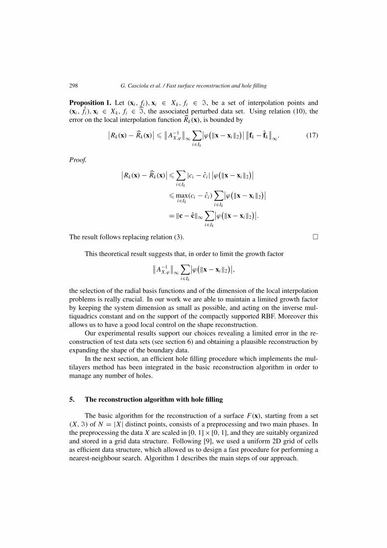
Figure 5. Reconstructed angel-h3 data set: (a) algorithm 1; (b) algorithm 2.
(a) (b) (c)
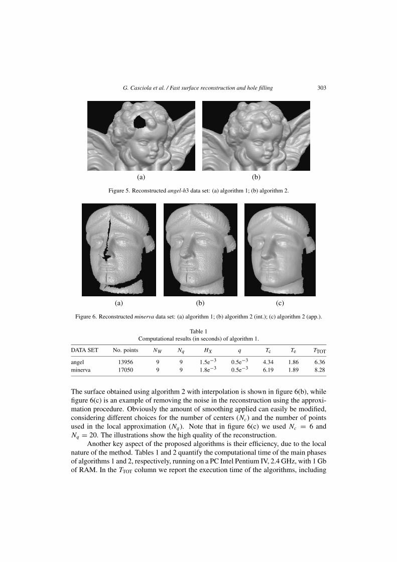
Figure 6. Reconstructed minerva data set: (a) algorithm 1; (b) algorithm 2 (int.); (c) algorithm 2 (app.).
Table 1Computational results (in seconds) of algorithm 1.
DATA SET No. points NW Nq HX q Tc Te TTOT
angel 13956 9 9 1.5e−3 0.5e−3 4.34 1.86 6.36minerva 17050 9 9 1.8e−3 0.5e−3 6.19 1.89 8.28
The surface obtained using algorithm 2 with interpolation is shown in figure 6(b), whilefigure 6(c) is an example of removing the noise in the reconstruction using the approxi-mation procedure. Obviously the amount of smoothing applied can easily be modified,considering different choices for the number of centers (Nc) and the number of pointsused in the local approximation (Nq). Note that in figure 6(c) we used Nc = 6 andNq = 20. The illustrations show the high quality of the reconstruction.
Another key aspect of the proposed algorithms is their efficiency, due to the localnature of the method. Tables 1 and 2 quantify the computational time of the main phasesof algorithms 1 and 2, respectively, running on a PC Intel Pentium IV, 2.4 GHz, with 1 Gbof RAM. In the TTOT column we report the execution time of the algorithms, including

304 G. Casciola et al. / Fast surface reconstruction and hole filling
Table 2Computational results (in seconds) of algorithm 2.
DATA SET No. points NW Nq HX q Tc Thf Te TTOT
angel-h1 13856 9 9 1.5e−3 0.5e−3 4.30 2.78 2.06 9.34angel-h2 13583 9 9 1.5e−3 0.5e−3 4.19 11.08 2.56 18.11angel-h3 13783 9 9 1.5e−3 0.5e−3 4.27 5.90 2.25 12.63minerva (int) 17050 9 9 1.8e−3 0.5e−3 6.18 12.16 5.00 23.66minerva (app) 17050 20 20 1.8e−3 0.5e−3 8.17 14.05 5.02 27.23
the preprocessing phase, while the Tc, Thf and Te report the computational time of thecoefficient, the hole filling and the evaluation phases, respectively. The latter stronglydepends on the evaluation grid used; all the reconstructed surfaces we considered havebeen evaluated in a 300 × 300 uniform grid.
In the tables we also report the free parameters NW , Nq , the separation distance q
and the estimated density HX of the data sets. Note that the latter corresponds to theacquisition step of the scanner and its value represents the fill distance of the local inter-polation problems and it has been used to estimate the separation distance q. This hasallowed us to satisfy the quasi-uniformity conditions (8), guaranteeing a compromisebetween stability and quality. In fact, the uniformity parameter ρ of the sets Xk turns outto be ρ � 0.67 for the angel data set and ρ � 0.55 for the minerva data set. Note that,in the minerva data set, we could have considered a slightly bigger value for q yieldinga bigger density value, but the algorithm would have been less efficient.
Acknowledgements
This work has been supported by MIUR-Cofin 2002. We are grateful to Ing. S.Petronilli (ENEA, Bologna) for providing the data and motivation for this research. Wealso thank the referees for many useful comments.
References
[1] C.L. Bajaj, F. Bernardini and G. Xu, Automatic reconstruction of surfaces and scalar fields from 3Dscans, in: Proc. of SIGGRAPH 1995 (ACM Press, New York, 1995).
[2] J.C. Carr, R.K. Beatson, J.B. Cherrie, T.J. Mitchell, W.R. Fright, B.C. McCallum and T.R. Evans,Reconstruction and representation of 3D objects with radial basis functions, in: Proc. of SIGGRAPH2001 (ACM Press, New York, 2001) pp. 67–76.
[3] J. Davis, S.R. Marshner, M. Garr and M. Levoy, Filling holes in complex surfaces using volumetricdiffusion, in: Proc. of the First Internat. Symposium on 3D Data Processing, Visualization, Transmis-sion (2001).
[4] M.S. Floater and A. Iske, Multistep scattered data interpolation using compactly supported radialbasis functions, J. Comput. Appl. Math. 73(5) (1996) 65–78.
[5] W.J. Gordon and J.A. Wixson, Shepard’s method of metric interpolation to bivariate and multivariateinterpolation, Math. Comp. 32(141) (1978) 253–264.

G. Casciola et al. / Fast surface reconstruction and hole filling 305
[6] H. Hoppe, T. DeRose, T. Duchamp, J. McDonald and W. Stuetzle, Surface reconstruction from unor-ganized points, in: Proc. of SIGGRAPH 1992 (ACM Press, New York, 1992).
[7] D. Lazzaro and L.B. Montefusco, Radial basis functions for the multivariate interpolation of largescattered data sets, J. Comput. Appl. Math. 140 (2002) 521–536.
[8] W.R. Madich and S.A. Nelson, Bounds on multivariate polynomials and exponential error estimatesfor multiquadric interpolation, J. Approx. Theory 70 (1992) 94–114.
[9] R.J. Renka, Multivariate interpolation of large sets of scattared data, ACM Trans. Math. Software14(2) (1988) 139–148.
[10] R. Schaback, Creating surfaces from scattared data using radial basis functions, in: MathematicalMethods for Curves and Surfaces, eds. M. Daehlen, T. Lyche and L. Schumaker (Vanderbilt Univ.Press, Nashville, TN, 1995) 477–496.
[11] R. Schaback, Error estimates and condition numbers for radial basis function interpolation, Adv.Comput. Math. 3 (1995) 251–264.
[12] H. Wendland, Error estimates for interpolation by compactly supported radial basis functions of min-imal degree, J. Approx. Theory 93 (1998) 258–272.
[13] H. Wendland, Piecewise polynomial, positive definite and compactly supported radial functions ofminimal degree, Adv. Comput. Math. 4 (1995) 359–396.
[14] Z. Wu, Multivariate compactly supported positive definite radial functions, Adv. Comput. Math. 4(1995) 283–292.