Fast Polygonal Approximation ofTerrains and Height Fields

Michael Garland and Paul S. Heckbert

September 19, 1995

CMU-CS-95-181

School of Computer ScienceCarnegie Mellon University

Pittsburgh, PA 15213

email: {garland,ph}@cs.cmu.edutech report & C++ code: http://www.cs.cmu.edu/˜garland/scape

This work was supported by ARPA contract F19628-93-C-0171 and NSF Young Investigator award CCR-9357763.The views and conclusions contained in this document are those of the authors and should not be interpreted asrepresenting the official policies, either expressed or implied, of ARPA, NSF, or the U.S. government.

Keywords: surface simplification, surface approximation, surface fitting, Delaunay triangula-tion, data-dependent triangulation, triangulated irregular network, TIN, multiresolution modeling,level of detail, greedy insertion.

Abstract

Several algorithms for approximating terrains and other height fields using polygonal meshes aredescribed, compared, and optimized. These algorithms take a height field as input, typically arectangular grid of elevation data H(x, y), and approximate it with a mesh of triangles, also knownas a triangulated irregular network, or TIN. The algorithms attempt to minimize both the errorand the number of triangles in the approximation. Applications include fast rendering of terraindata for flight simulation and fitting of surfaces to range data in computer vision. The methodscan also be used to simplify multi-channel height fields such as textured terrains or planar colorimages.

The most successful method we examine is the greedy insertion algorithm. It begins with a simpletriangulation of the domain and, on each pass, finds the input point with highest error in the currentapproximation and inserts it as a vertex in the triangulation. The mesh is updated either withDelaunay triangulation or with data-dependent triangulation. Most previously published variantsof this algorithm had expected time cost of O(mn) or O(n logm+m2), where n is the number ofpoints in the input height field and m is the number of vertices in the triangulation. Our optimizedalgorithm is faster, with an expected cost of O((m+n) logm). On current workstations, this allowsone million point terrains to be simplified quite accurately in less than a minute. We are releasinga C++ implementation of our algorithm.

Contents

1. Introduction . . . . . . . . . . . . . . . . . . 12. Statement of Problem and Approach . . . . 23. Importance Measures . . . . . . . . . . . . . 44. Greedy Insertion . . . . . . . . . . . . . . . 7

Algorithm I . . . . . . . . . . . . . . . . . 8Algorithm II . . . . . . . . . . . . . . . . . 11Algorithm III . . . . . . . . . . . . . . . . 13Algorithm IV . . . . . . . . . . . . . . . . 18

5. Results . . . . . . . . . . . . . . . . . . . . . 226. Ideas for Future Research . . . . . . . . . . 307. Summary . . . . . . . . . . . . . . . . . . . 328. Acknowledgements . . . . . . . . . . . . . . 349. References . . . . . . . . . . . . . . . . . . . 34

1. Introduction

A height field is a set of height samples over a planar domain. Terrain data, a common type ofheight field, is used in many applications, including flight simulators, ground vehicle simulators, andin computer graphics for entertainment. Computer vision uses height fields to represent range dataacquired by stereo and laser range finders. In all of these applications, an efficient data structurefor representing and displaying the height field is desirable.

Our primary motivation is to render height field data rapidly and with high fidelity. Since almostall graphics hardware uses the polygon as the fundamental building block for object description, itseems natural to represent the terrain as a mesh of polygonal elements. The raw sample data canbe trivially converted into polygons by placing edges between each pair of neighboring samples.However, for terrains of any significant size, rendering the full model is prohibitively expensive.For example, the 2,000,000 triangles in a 1, 000×1, 000 grid take about seven seconds to render oncurrent graphics workstations, which can display roughly 10,000 triangles in real time (every 30th ofa second). Even as the fastest graphics workstations speed up in coming years, typical workstationsand personal computers will remain far slower. More fundamentally, the detail of the full model ishighly redundant when it is viewed from a distance, and its use in such cases is unnecessary andwasteful. Many terrains have large, nearly planar regions which are well approximated by largepolygons. Ideally, we would like to render models of arbitrary height fields with just enough detailfor visual accuracy. Additionally, in systems which are highly constrained, we would like to use aless detailed model in order to conserve memory, disk space, or network bandwidth.

To render a height field quickly, we can use multiresolution modeling, preprocessing it to con-struct approximations of the surface at various levels of detail [3, 16]. When rendering the heightfield, we can choose an approximation with an appropriate level of detail and use it in place of theoriginal. The various levels of detail can be combined into a hierarchical triangulation [6, 5].

In some applications, such as flight simulators, the speed of simplification is unimportant, be-cause database preparation is done off-line, once, while rendering of the simplified terrain is donethousands of times. In more general computer graphics and computer animation applications, thescene being simplified might be changing many times per second, however, so a slow simplificationmethod might be useless. Finding a simplification algorithm that is fast is therefore quite important

1

to us.

Our focus in this paper will be to generate simplified models of a height field from the originalmodel. The simplified model should accurately approximate the original model, use as few trianglesas possible, and the process of simplification should be as rapid as possible.

The remainder of this paper contains the following sections: We begin by stating the problemwe are solving. Next we describe several methods for selecting the most important points of aheight field. The core of the paper is the following section on the greedy insertion algorithm, wherewe begin with the basic algorithm, and through a progression of simple optimizations, speed it updramatically. We explore the use of both Delaunay triangulation and data-dependent triangulation.The paper concludes with a discussion of empirical results, ideas for future work, and a summary.

1.1. Background

Our companion survey paper [17] contains a thorough review of surface simplification methods. Tosummarize, algorithms for polygonal simplification of surfaces can be categorized into six groups:

• uniform grid methods, which use a regular grid of samples in x and y;

• hierarchical subdivision methods, which are based on quadtree, k-d tree, and hierarchicaltriangulations;

• one pass feature methods, which select a set of important “feature” points (such as peaks,pits, ridges, and valleys) in one pass and use them as the vertex set for triangulation;

• multi-pass refinement methods which start with a minimal approximation and use multiplepasses of point selection and retriangulation to build up the final triangulation;

• multi-pass decimation methods, which begin with a triangulation of all of the input points anditeratively delete vertices from the triangulation, gradually simplifying the approximation;and

• other methods, including adjustment techniques, optimization-based methods, and optimalmethods.

The latter four simplification methods typically employ general triangulations that are neitheruniform nor hierarchical. Two such general triangulation methods are Delaunay triangulation anddata-dependent triangulation.

Delaunay triangulation is a purely two-dimensional method; it uses only the xy projections ofthe input points. It finds a triangulation that maximizes the minimum angle of all triangles, amongall triangulations of a given point set [13, 21]. This helps to minimize the occurrence of very thinsliver triangles. Data-dependent triangulation, in contrast, uses the heights of points in additionto their x and y coordinates [8, 31]. It can achieve lower error approximations than Delaunaytriangulation, but it generates more slivers.

2. Statement of Problem and Approach

We assume that a discrete two-dimensional set of samples H of some underlying surface isprovided. This is most naturally represented as a discrete function where H(x, y) = z means

2

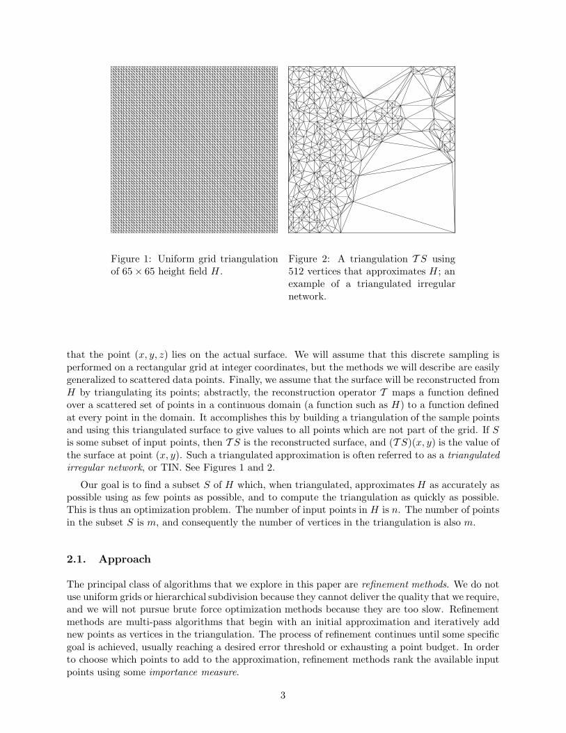
Figure 1: Uniform grid triangulationof 65× 65 height field H .

Figure 2: A triangulation T S using512 vertices that approximates H ; anexample of a triangulated irregularnetwork.

that the point (x, y, z) lies on the actual surface. We will assume that this discrete sampling isperformed on a rectangular grid at integer coordinates, but the methods we will describe are easilygeneralized to scattered data points. Finally, we assume that the surface will be reconstructed fromH by triangulating its points; abstractly, the reconstruction operator T maps a function definedover a scattered set of points in a continuous domain (a function such as H) to a function definedat every point in the domain. It accomplishes this by building a triangulation of the sample pointsand using this triangulated surface to give values to all points which are not part of the grid. If Sis some subset of input points, then T S is the reconstructed surface, and (T S)(x, y) is the value ofthe surface at point (x, y). Such a triangulated approximation is often referred to as a triangulatedirregular network, or TIN. See Figures 1 and 2.

Our goal is to find a subset S of H which, when triangulated, approximates H as accurately aspossible using as few points as possible, and to compute the triangulation as quickly as possible.This is thus an optimization problem. The number of input points in H is n. The number of pointsin the subset S is m, and consequently the number of vertices in the triangulation is also m.

2.1. Approach

The principal class of algorithms that we explore in this paper are refinement methods. We do notuse uniform grids or hierarchical subdivision because they cannot deliver the quality that we require,and we will not pursue brute force optimization methods because they are too slow. Refinementmethods are multi-pass algorithms that begin with an initial approximation and iteratively addnew points as vertices in the triangulation. The process of refinement continues until some specificgoal is achieved, usually reaching a desired error threshold or exhausting a point budget. In orderto choose which points to add to the approximation, refinement methods rank the available inputpoints using some importance measure.

3

In exploring importance measures, we reject those that make use of implicit knowledge aboutthe nature of terrains, such as the existence of ridge lines. We would like our algorithms to applyto general height fields, where assumptions that are valid for terrains might fail. Even if we wereto constrain ourselves to terrains alone, we are not aware of conclusive evidence suggesting thathigh fidelity results (as measured by an objective L2 or L∞ metric1) require high level knowledgeof terrains.

3. Importance Measures

Within the basic framework outlined above, the key to good simplification lies in the choice ofa good point importance measure. But what criteria should be used to judge such a measure?Ultimately, the final judgement must depend upon the quality of the results it produces. With thisin mind, we suggest that a good measure should be simple and fast, it should produce good resultson arbitrary height fields, and it should use only local information. The requirement that a measurebe simple and fast is easy to justify; since we will be simplifying detailed terrains and height fields,the importance measure will be evaluated many times. Consequently, any cost inherent in theimportance measure will be magnified many times due to its repetition. We also demand thatthe measure apply equally well to all height fields whether they are terrains, colored textures,or other semi-continuous functions. This becomes increasingly important for the simplification ofheight fields with color texture or other material properties, which we will discuss later. Measureswhich depend on characteristics peculiar to terrains or any other specific kind of height field, areunacceptable to us. Finally, the importance measure should use only local information. Thisrequirement is necessary to support some significant optimizations in the algorithm’s running time.

We explored four categories of importance measures: local error, curvature, global error, andproducts of selected other measures. We briefly discuss each of these below.

3.1. Local Error Measure

The first measure which we explored is simple vertical error. The importance of a point (x, y) ismeasured as the difference between the actual function and the interpolated approximation at thatpoint (i.e. |H(x, y)− (T S)(x, y)|. This difference is a measure of local error. Intuitively, we wouldexpect that eliminating such local errors would yield high quality approximations, and it generallydoes. This measure also meets the other criteria suggested earlier: it is simple, fast, and uses onlylocal information.

3.2. Curvature Measure

The piecewise-linear reconstruction effected by T approximates nearly planar functions well, butdoes more poorly on curved surfaces. However, in everyday life, peaks, pits, ridges, and valleys,which have high curvature, are visually significant. These observations suggest that we try curvatureas a measure of importance.

1In this paper, we use the following error metrics: We define the L2 error between two n-vectors u and v as

||u − v||2 =[∑n

i=1(ui − vi)2

]1/2. The L∞ error, also called the maximum error, is ||u − v||∞ = maxni=1 |ui − vi|.

We define the squared error to be the square of the L2 error, and the root mean square or RMS error to be the L2

error divided by√n. Optimization with respect to the L2 and L∞ metrics are called least squares and minimax

optimization, and we call such solutions L2–optimal and L∞–optimal, respectively.

4

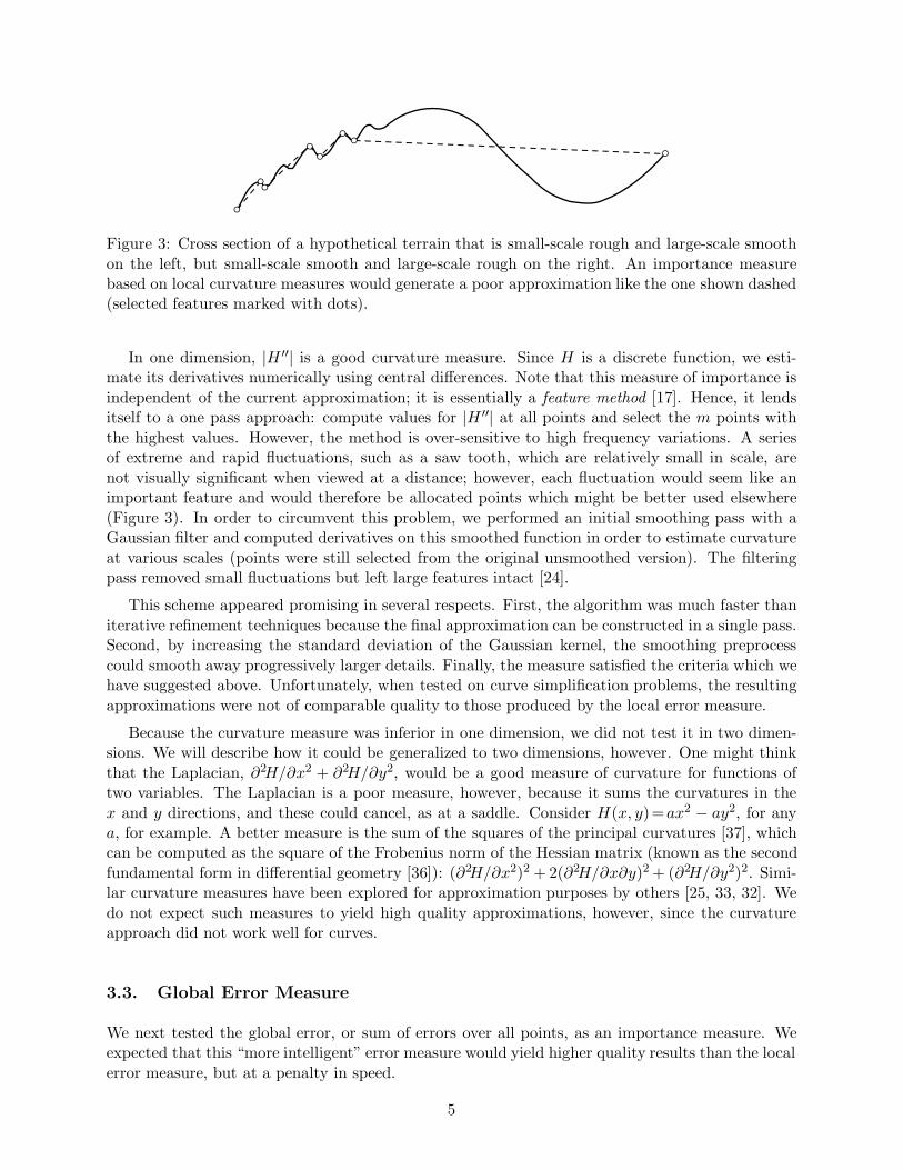
Figure 3: Cross section of a hypothetical terrain that is small-scale rough and large-scale smoothon the left, but small-scale smooth and large-scale rough on the right. An importance measurebased on local curvature measures would generate a poor approximation like the one shown dashed(selected features marked with dots).

In one dimension, |H ′′| is a good curvature measure. Since H is a discrete function, we esti-mate its derivatives numerically using central differences. Note that this measure of importance isindependent of the current approximation; it is essentially a feature method [17]. Hence, it lendsitself to a one pass approach: compute values for |H ′′| at all points and select the m points withthe highest values. However, the method is over-sensitive to high frequency variations. A seriesof extreme and rapid fluctuations, such as a saw tooth, which are relatively small in scale, arenot visually significant when viewed at a distance; however, each fluctuation would seem like animportant feature and would therefore be allocated points which might be better used elsewhere(Figure 3). In order to circumvent this problem, we performed an initial smoothing pass with aGaussian filter and computed derivatives on this smoothed function in order to estimate curvatureat various scales (points were still selected from the original unsmoothed version). The filteringpass removed small fluctuations but left large features intact [24].

This scheme appeared promising in several respects. First, the algorithm was much faster thaniterative refinement techniques because the final approximation can be constructed in a single pass.Second, by increasing the standard deviation of the Gaussian kernel, the smoothing preprocesscould smooth away progressively larger details. Finally, the measure satisfied the criteria which wehave suggested above. Unfortunately, when tested on curve simplification problems, the resultingapproximations were not of comparable quality to those produced by the local error measure.

Because the curvature measure was inferior in one dimension, we did not test it in two dimen-sions. We will describe how it could be generalized to two dimensions, however. One might thinkthat the Laplacian, ∂2H/∂x2 + ∂2H/∂y2, would be a good measure of curvature for functions oftwo variables. The Laplacian is a poor measure, however, because it sums the curvatures in thex and y directions, and these could cancel, as at a saddle. Consider H(x, y)=ax2 − ay2, for anya, for example. A better measure is the sum of the squares of the principal curvatures [37], whichcan be computed as the square of the Frobenius norm of the Hessian matrix (known as the secondfundamental form in differential geometry [36]): (∂2H/∂x2)2 + 2(∂2H/∂x∂y)2 + (∂2H/∂y2)2. Simi-lar curvature measures have been explored for approximation purposes by others [25, 33, 32]. Wedo not expect such measures to yield high quality approximations, however, since the curvatureapproach did not work well for curves.

3.3. Global Error Measure

We next tested the global error, or sum of errors over all points, as an importance measure. Weexpected that this “more intelligent” error measure would yield higher quality results than the localerror measure, but at a penalty in speed.

5

At every point, we compute the global resultant error of a new approximation formed by addingthat point to the current approximation, measured as

∑x,y |H(x, y)− (T S)(x, y)|. Then we merely

select the point that produces the smallest global error. This approach is similar to one movelook-ahead in game playing algorithms, or hill climbing. Compared to the local error measure,instead of simply assuming that the addition of points of high local error will in fact decrease theglobal error, it chooses the point which actually minimizes the global error. This measure violatesone of our stated criteria; it is not local. However, it seemed that this approach might give betterresults than the previous measure.

The algorithm would seem prohibitively expensive, but it is not, at least in one dimension. Ifyou are willing to sacrifice O(n) space and time to precompute several partial sum arrays, theglobal error resulting after the introduction of a point can be computed in constant time.

When tested on curves, the global error measure yielded poor results. This was surprising, sincewe had expected it to yield better results than the simpler local error measure. This is simplyan instance of a standard problem with hill climbing optimization methods: they are too shortsighted. It is often necessary to make several “bad” moves in the short term to achieve long termsuccess. In our case, accurately fitting a particular feature might require the addition of at leasttwo points. It is quite possible that introducing the first point will introduce significant error whichwill be eradicated by introducing the second point. The global error measure is too conservative;it is too concerned with the immediate consequences of inserting any particular point and notknowledgeable enough to see possible future benefits from this action. While it might be possibleto fix this behavior using a standard technique such as simulated annealing, this would only furtherincrease the cost of this already expensive algorithm. It appears unlikely that this high expensewould produce correspondingly better results than those achieved using the simpler local errormeasure.

A second problem with the global error measure is that there does not appear to be a general-ization of the partial sum trick that would permit errors over triangles to be computed in constanttime.

3.4. Product Measures

The last approach to measuring importance which we explored was another attempt to improveupon the local error measure. One would think that this could be improved upon using a moreinformed heuristic function. We tested the performance of a set of related measures formed bythe product of several simpler measures2. The method we used was to combine one or more ofthe importance measures given above with some bias measures. Two examples of bias measuresare: absolute height, and the ratio of the number of unselected points in a region to the numberof points remaining to be selected. Using these product measures, we were able to achieve resultswhich were only slightly poorer than those produced by the local error measure. However, productmeasures are more complex, and hence more expensive, than any of the measures discussed so farwith the exception of global error. Thus, the resulting algorithm was significantly slower.

2We use products rather than sums because the units of measure of the constituent terms are generally unrelated.Thus, simple summation does not yield meaningful information.

6

3.5. Decimation Algorithms

We next investigated decimation variants of two of these measures. The curvature measure hasno decimation variant since it is not iterative, and decimation with the local error measure isessentially the same as Lee’s drop heuristic algorithm [22].

We tested decimation variants of the global error measure and the product measure on curves.The results were interesting, but ultimately poorer than other methods. We found that the globalerror measure produced more accurate approximations when used in a decimation algorithm thanin a refinement algorithm. Proceeding from a detailed approximation to a cruder one amelioratedthe problems of the global error measure; in a decimation algorithm there seems to be less need tolook several moves ahead. Thus, if the algorithm simply removes the point whose absence adds thesmallest error to the approximation, this will lead to a good approximation in most cases. Productmeasures incorporating the global error measure also performed better in a decimation algorithm,but the performance of other product measures was essentially unchanged. However, the results ofthese decimation algorithms were still slightly less accurate than those produced by the local errormeasure.

3.6. Conclusions from Importance Measure Experiments

Importance measures which make no reference to the approximation (such as most feature methods)were not very successful in our experiments. A fundamental flaw of most such methods is thatthey give no guarantee about the accuracy of their approximations. The cause of this low qualityseems to be the independence and locality of decisions made by most of these algorithms.

A terrain that is rough at a small scale but nearly planar at a large scale (e.g., a city) willhave many high-importance points, while a terrain that is smooth at a small scale and rough at alarge scale (e.g., rolling hills) will have few. If these two terrain types are both present in a singledataset, too many features will be devoted to regions of the first type and too few to the latter,leading to poor simplification, as shown in Figure 3. The methods behave poorly in the presenceof noisy height data for similar reasons.

After empirical comparison of results from the above methods, we settled on the local errormeasure for iterative refinement. We found that it was the simplest to implement, produced moreaccurate results than any of our alternatives, and was faster than all but the curvature measure.We will demonstrate in the following sections that this algorithm is easily generalized to othersimplification problems, and that it can be fast.

4. Greedy Insertion

We call refinement algorithms that insert the point(s) of highest error on each pass greedy insertionalgorithms, “greedy” because they make irrevocable decisions as they go [4], and “insertion” becauseon each pass they insert one or more vertices into the triangulation. Methods that insert a singlepoint in each pass we call sequential greedy insertion and methods that insert multiple points inparallel on each pass we call parallel greedy insertion. The words “sequential” and “parallel” hererefer to the selection and re-evaluation process, not to the architecture of the machine. Manyvariations on the greedy insertion algorithm have been explored over the years; apparently thealgorithm has been reinvented many times [10, 7, 18, 31, 28, 11, 30].

We now explore four variants of the sequential greedy insertion algorithm. Our first method,

7

algorithm I, is a brute force implementation of sequential greedy insertion with Delaunay triangu-lation. This algorithm is quite slow, so we present two optimizations. Algorithm II exploits thelocality of changes to the triangulation to eliminate redundant recalculation of error, and algo-rithm III goes further, employing better data structures to speed selection of the point of highesterror. The result is an algorithm that computes high quality approximations very rapidly. Next, wetake this algorithm and replace Delaunay triangulation with data-dependent triangulation, yieldingalgorithm IV, which generates slightly higher quality approximations than algorithm III.

4.1. Basic Algorithm

We begin with some basic functions that query the Delaunay mesh3 and perform incrementalDelaunay triangulation. The routine Mesh Insert locates the triangle containing a given point,splits the triangle into three, and then recursively checks each of the outer edges of these triangles,flipping them if necessary to maintain a Delaunay triangulation (Figure 4) [13].

Mesh Insert(Point p): Insert p as a vertex in the Delaunay mesh

Mesh Locate(Point p): Find the triangle in the mesh containing point p

Locate and Interpolate(Point p): Locate the triangle containing point p and interpolate there

Insert(Point p ):mark p as usedMesh Insert(p)

Error(Point p ):% Returns the error at a point (our importance measure)return |H(p)− Locate and Interpolate(p)|

The heart of the algorithm is sequential greedy insertion, much as described in earlier work[7, 31, 11]. It is simple and unoptimized. We build an initial approximation of two triangles usingthe corner points of H . Then we repeatedly scan the unused points to find the one with the largesterror and call Insert to add it to the current approximation. The conditions for terminationare stated abstractly as a function Goal Met; they would typically be based on the number ofpoints selected, the maximum (L∞) error of the approximation, or the squared (L2) error of theapproximation.

3The terms “mesh” and “triangulation” are used synonymously henceforth.

8

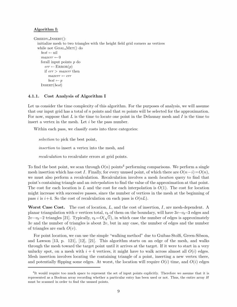
Algorithm I:

Greedy Insert():initialize mesh to two triangles with the height field grid corners as verticeswhile not Goal Met() do

best ← nilmaxerr ← 0forall input points p do

err ←Error(p)if err > maxerr then

maxerr ← errbest ← p

Insert(best)

4.1.1. Cost Analysis of Algorithm I

Let us consider the time complexity of this algorithm. For the purposes of analysis, we will assumethat our input grid has a total of n points and that m points will be selected for the approximation.For now, suppose that L is the time to locate one point in the Delaunay mesh and I is the time toinsert a vertex in the mesh. Let i be the pass number.

Within each pass, we classify costs into three categories:

selection to pick the best point,

insertion to insert a vertex into the mesh, and

recalculation to recalculate errors at grid points.

To find the best point, we scan through O(n) points4 performing comparisons. We perform a singlemesh insertion which has cost I . Finally, for every unused point, of which there are O(n−i)=O(n),we must also perform a recalculation. Recalculation involves a mesh location query to find thatpoint’s containing triangle and an interpolation to find the value of the approximation at that point.The cost for each location is L and the cost for each interpolation is O(1). The cost for locationmight increase with successive passes, since the number of vertices in the mesh at the beginning ofpass i is i+4. So the cost of recalculation on each pass is O(nL).

Worst Case Cost. The cost of location, L, and the cost of insertion, I , are mesh-dependent. Aplanar triangulation with v vertices total, vb of them on the boundary, will have 3v−vb−3 edges and2v−vb−2 triangles [21]. Typically, vb=O(

√v), in which case the number of edges is approximately

3v and the number of triangles is about 2v, but in any case, the number of edges and the numberof triangles are each O(v).

For point location, we can use the simple “walking method” due to Guibas-Stolfi, Green-Sibson,and Lawson [13, p. 121], [12], [21]. This algorithm starts on an edge of the mesh, and walksthrough the mesh toward the target point until it arrives at the target. If it were to start in a veryunlucky spot, on a mesh with i + 4 vertices, it might have to walk across almost all O(i) edges.Mesh insertion involves locating the containing triangle of a point, inserting a new vertex there,and potentially flipping some edges. At worst, the location will require O(i) time, and O(i) edges

4It would require too much space to represent the set of input points explicitly. Therefore we assume that it isrepresented as a Boolean array recording whether a particular entry has been used or not. Thus, the entire array Hmust be scanned in order to find the unused points.

9

will need to be flipped. So mesh location and insertion can require time linear in the number ofpoints in the mesh, and L=I=O(i).

Thus, in the worst case, the costs per pass for algorithm I are: O(n) for selection, O(i) forinsertion, and O(in) for recalculation. The asymptotically dominant term is recalculation, so thetotal worst case cost is

∑mi=1 O(in) = O(m2n).

Expected Case Cost. Fortunately, the worst case behavior is very unlikely. In practice, it is theexpected cost behavior which we observe. So the expected cost is a much more important measureof the practical speed of the algorithm.

The expected cost for random access location queries in a Delaunay mesh with v vertices fortypical point distributions is only L=O(

√v) [13, 14]. However, if successive location queries are

close together, then the location procedure can start its search at the triangle returned by theprevious call so that very few steps will be needed to find the next target point. In this situation,the expected cost of location is L=O(1) [13].

In the algorithm above, point location queries almost always occur near one another. All but afew of them are made in the process of scanning the unused points. Since this scanning proceedsacross each row in order, successively scanned points are almost always nearby and are usually directneighbors. Of course, it is possible to construct meshes in which both insertion and location willhave linear cost. We cannot guarantee that this will never happen, but the conditions under whichthis behavior might arise are very uncommon. In the course of our experiments, this degeneracyhas never yet occurred in practice. So the expected cost of location during recalculation is L=O(1).

Insertion involves a location query that usually does not exhibit as much spatial coherence aslocation queries due to recalculation, so its expected cost in this context is L=O(

√i). The other

costs of insertion are due to edge flips. On average, the number of edge flips is constant, and eachtakes constant time, with Delaunay triangulation, so the expected cost for insertions is I=O(

√i).

Assuming L=O(1) and I=O(√i) in the expected case, the costs per pass for algorithm I are:

O(n) for selection, O(√i) for insertion, and O(n) for recalculation. The asymptotically dominant

terms are selection and recalculation, so the total expected case cost is∑mi=1 O(n) = O(mn).

4.2. Faster Recalculation

The algorithm above yields high quality results. However, even our expected time complexity esti-mate of O(mn) is expensive, and the worst case complexity of O(m2n) is exorbitant. Fortunately,we can improve upon our original naive algorithm considerably by exploiting the locality of thechanges to the approximation during incremental Delaunay triangulation.

4.2.1. Delaunay Triangulation

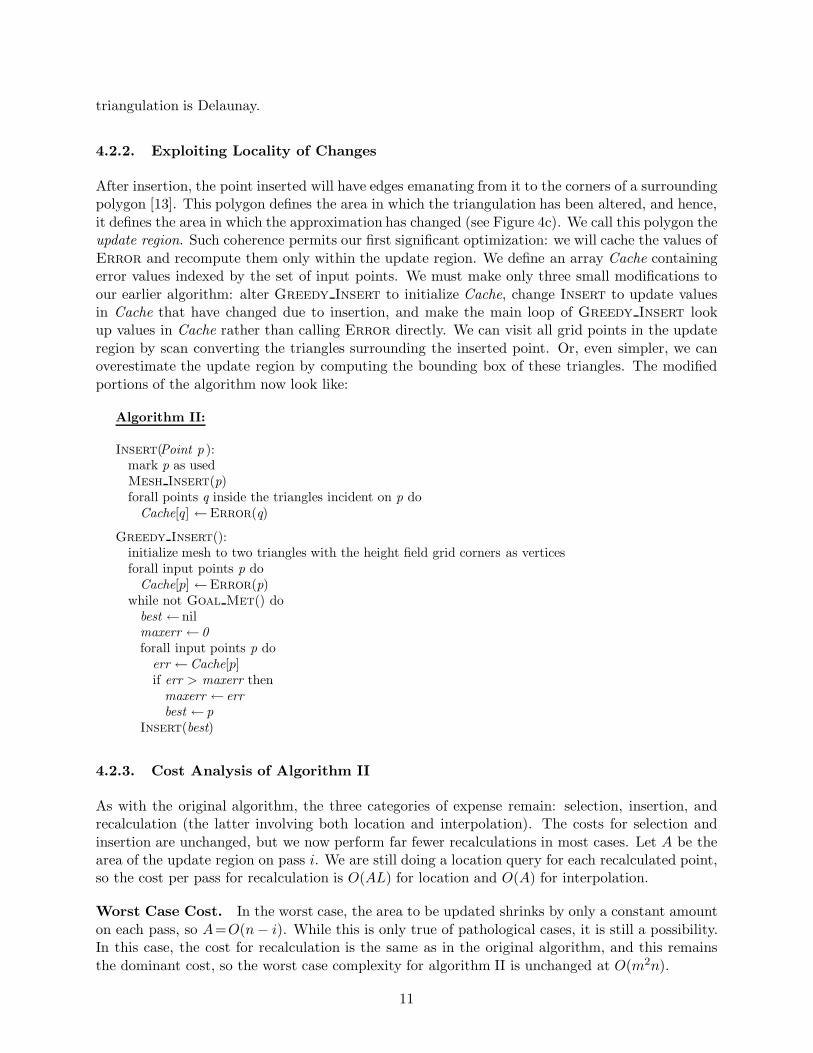
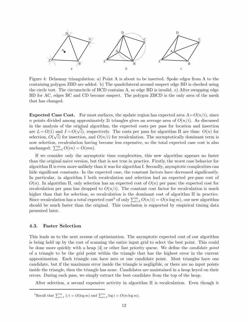
The incremental Delaunay triangulation algorithm is illustrated in Figure 4, and works as follows[13, 21]: To insert a vertex A, locate its containing triangle, or, if it lies on an edge, delete thatedge and find its containing quadrilateral. Add “spoke” edges from A to the vertices of thiscontaining polygon. All perimeter edges of the containing polygon are suspect and their validitymust be checked. An edge is valid iff it passes the circle test: if A lies outside the circumcircle ofthe triangle that is on the opposite side of the edge from A. All invalid edges must be swappedwith the other diagonal of the quadrilateral containing them, at which point the containing polygonacquires two new suspect edges. The process continues until no suspect edges remain. The resulting

10

triangulation is Delaunay.

4.2.2. Exploiting Locality of Changes

After insertion, the point inserted will have edges emanating from it to the corners of a surroundingpolygon [13]. This polygon defines the area in which the triangulation has been altered, and hence,it defines the area in which the approximation has changed (see Figure 4c). We call this polygon theupdate region. Such coherence permits our first significant optimization: we will cache the values ofError and recompute them only within the update region. We define an array Cache containingerror values indexed by the set of input points. We must make only three small modifications toour earlier algorithm: alter Greedy Insert to initialize Cache, change Insert to update valuesin Cache that have changed due to insertion, and make the main loop of Greedy Insert lookup values in Cache rather than calling Error directly. We can visit all grid points in the updateregion by scan converting the triangles surrounding the inserted point. Or, even simpler, we canoverestimate the update region by computing the bounding box of these triangles. The modifiedportions of the algorithm now look like:

Algorithm II:

Insert(Point p ):mark p as usedMesh Insert(p)forall points q inside the triangles incident on p do

Cache[q] ←Error(q)

Greedy Insert():initialize mesh to two triangles with the height field grid corners as verticesforall input points p do

Cache[p] ←Error(p)while not Goal Met() do

best ← nilmaxerr ← 0forall input points p do

err ←Cache[p]if err > maxerr then

maxerr ← errbest ← p

Insert(best)

4.2.3. Cost Analysis of Algorithm II

As with the original algorithm, the three categories of expense remain: selection, insertion, andrecalculation (the latter involving both location and interpolation). The costs for selection andinsertion are unchanged, but we now perform far fewer recalculations in most cases. Let A be thearea of the update region on pass i. We are still doing a location query for each recalculated point,so the cost per pass for recalculation is O(AL) for location and O(A) for interpolation.

Worst Case Cost. In the worst case, the area to be updated shrinks by only a constant amounton each pass, so A=O(n− i). While this is only true of pathological cases, it is still a possibility.In this case, the cost for recalculation is the same as in the original algorithm, and this remainsthe dominant cost, so the worst case complexity for algorithm II is unchanged at O(m2n).

11

★A

Z

D

A

B

C

D

B

C

Z

a b

D

A

B

C

Z

c

Figure 4: Delaunay triangulation: a) Point A is about to be inserted. Spoke edges from A to thecontaining polygon ZBD are added. b) The quadrilateral around suspect edge BD is checked usingthe circle test. The circumcircle of BCD contains A, so edge BD is invalid. c) After swapping edgeBD for AC, edges BC and CD become suspect. The polygon ZBCD is the only area of the meshthat has changed.

Expected Case Cost. For most surfaces, the update region has expected area A=O(n/i), sincen points divided among approximately 2i triangles gives an average area of O(n/i). As discussedin the analysis of the original algorithm, the expected costs per pass for location and insertionare L=O(1) and I =O(

√i), respectively. The costs per pass for algorithm II are thus: O(n) for

selection, O(√i) for insertion, and O(n/i) for recalculation. The asymptotically dominant term is

now selection, recalculation having become less expensive, so the total expected case cost is alsounchanged:

∑mi=1O(in) = O(mn).

If we consider only the asymptotic time complexities, this new algorithm appears no fasterthan the original naive version, but that is not true in practice. Firstly, the worst case behavior foralgorithm II is even more unlikely than it was for algorithm I. Secondly, asymptotic complexities canhide significant constants. In the expected case, the constant factors have decreased significantly.In particular, in algorithm I both recalculation and selection had an expected per-pass cost ofO(n). In algorithm II, only selection has an expected cost of O(n) per pass; the expected cost forrecalculation per pass has dropped to O(n/i). The constant cost factor for recalculation is muchhigher than that for selection, so recalculation is the dominant cost of algorithm II in practice.Since recalculation has a total expected cost5 of only

∑mi=1O(n/i) = O(n logm), our new algorithm

should be much faster than the original. This conclusion is supported by empirical timing datapresented later.

4.3. Faster Selection

This leads us to the next avenue of optimization. The asymptotic expected cost of our algorithmis being held up by the cost of scanning the entire input grid to select the best point. This couldbe done more quickly with a heap [4] or other fast priority queue. We define the candidate pointof a triangle to be the grid point within the triangle that has the highest error in the currentapproximation. Each triangle can have zero or one candidate point. Most triangles have onecandidate, but if the maximum error inside the triangle is negligible, or there are no input pointsinside the triangle, then the triangle has none. Candidates are maintained in a heap keyed on theirerrors. During each pass, we simply extract the best candidate from the top of the heap.

After selection, a second expensive activity in algorithm II is recalculation. Even though it

5Recall that∑m

i=11/i = O(logm) and

∑m

i=1log i = O(m logm).

12

doesn’t dominate the expected case complexity analysis, recalculation is very expensive in practicalterms. So far, the Error function used for recalculation has done a point location to find theenclosing triangle and an interpolation within the triangle. In our implementations of algorithmsI and II, interpolation is done by computing the plane defined by the three corners of the triangleand evaluating this plane equation at the specified point. All this is done each time a point’s erroris recalculated. Recalculation can be sped up in two ways. First, we can eliminate point locationaltogether, by recording with each candidate a pointer to its containing triangle. Second, we canspeed up interpolation by a constant factor by precomputing plane equations and caching themwith the triangle. As we scan convert a triangle, we track the best candidate seen so far.

4.3.1. Data Structures

Since the data structures are becoming more complex, we will describe them more precisely. Algo-rithm III, to be presented shortly, has the following primary data structures: planes, height fields,triangulations, and heaps. The plane data structure is little more than three coefficients a, b, andc for a plane equation H=ax+ by + c.

The height field consists of a rectangular array of points, each of which contains a height valueH(x, y), and a bit to record if the input point has been used by the triangulation.

For the triangulation, we use a slight modification to Guibas and Stolfi’s quad-edge data struc-ture [13], consisting of 2-D points, directed edges, and triangles in an interconnected graph. Eachedge points to neighboring edges and to a neighboring triangle. Triangles contain a pointer to oneof their edges, information about their candidate (its position candpos and a pointer into the heapheapptr) and the error over the triangle err. The pointer into the heap allows candidates to beupdated quickly and also allows fast retrieval of the candidate’s error.

The heap is a binary tree of records, each consisting of the candidate’s error and a pointer tothe triangle to which the candidate belongs. The latter information allows point location to bedone in constant time after the candidate of highest error is extracted from the heap.

Note that depending on the details of the point inclusion test used or the scan conversionalgorithm, points on an edge might be considered to be “inside” both of the adjacent triangles,in which case neighboring triangles might have identical candidates (see Figure 11). To avoidmultiple visits to edge points, one could use rational arithmetic during scan conversion. A carefulscan converter can also insure that vertices of the triangles are never visited. This can removethe need for the Boolean array of “used bits”, provided that they are not needed for any otherpurposes. In our experience, this is a minor detail; the algorithm will work whether edge pointsare multiply counted or not.

4.4. Optimized Delaunay Greedy Insertion

With selection speeded by a heap, location eliminated, and faster interpolation, our optimizedalgorithm is now:

13

Algorithm III: Delaunay Greedy Insertion:

HeapNode Heap Change(HeapNode h, float key, Triangle T ):% Set the key for heap node h to key, set its triangle pointer to T , and adjust heap.% Return (possibly new) heap node.if h 6= nil then

if key > 0 thenHeap Update(h, key)% update existing heap node

elseHeap Delete(h) % delete obsolete heap nodereturn nil

elseif key > 0 then

return Heap Insert(key, T)% insert new heap nodereturn h

Scan Triangle(Triangle T ):plane ←Find Triangle Plane(T)best ← nilmaxerr ← 0forall points p inside triangle T do

err ←|H(p)− Interpolate To Plane(p, plane)|if err > maxerr then

maxerr ← errbest ← p

T.heapptr ←Heap Change(T.heapptr, maxerr, T)T.candpos ← best

Mesh Insert(Point p, Triangle T): Insert a new vertex in triangle T , and update the Delaunay mesh

Insert(Point p, Triangle T ):mark p as usedMesh Insert(p, T) % incremental Delaunay triangulationforall triangles U adjacent to p do

Scan Triangle(U)

Greedy Insert():initialize mesh to two triangles with the height field grid corners as verticesforall initial triangles T do

Scan Triangle(T)while not Goal Met() do

T ←Heap Delete Max()Insert(T.candpos, T)

4.4.1. Cost Analysis of Algorithm III

Asymptotically, the most significant speedup relative to algorithm II is faster selection. In practice,optimization of interpolation is probably equally important.

In the new algorithm, time for selection is spent in three places: heap insertion, heap extraction,and heap updates. Clearly, the growth of the heap per pass is bounded by a constant, the netgrowth in the number of triangles, which is 2. However, the heap does not always grow this fast.In particular, as triangles become so small or so well fit to the height field as to have no candidate

14

Algorithm Selection Insertion RecalculationI O(n) O(i) O(in)II O(n) O(i) O(in)

III or IV O(log i) O(i) O(n)

Table 1: Worst case cost per pass, for pass i

points, they will be removed from the heap. The heap grows initially at 2 items per pass, andas refinement proceeds, the growth slows and eventually the heap will begin to shrink. Typically,the approximations that we wish to produce are much smaller than the original height fields.Consequently, the algorithm will rarely realize any significant benefit from shrinking heap sizes.We will simply assume that the size of the heap is O(i), and thus, that individual heap operationsrequire O(log i) time in an amortized sense.

The number of changes made to the heap per pass is 3 plus the number of edge flips performedduring mesh insertion. We assume that this is a small constant number. This is both reason-able and empirically confirmed on our sample data; in practice, the number of calls over time toHeap Change per pass is roughly 3–5. Given this assumption, the total heap cost, and henceselection cost, is O(log i) per pass.

The other two tasks, insertion and recalculation, are also cheaper now, since neither performslocations. The cost of recalculation has dropped from O(AL) to O(A).

Worst Case Time Cost. In the worst case, the insertion time is I=O(i) and the update areais A=O(n), so the costs per pass for algorithm III are: O(log i) for selection, O(i) for insertion,and O(n) for recalculation. The asymptotically dominant term is recalculation, as before, but it ismuch smaller now; the total worst case cost is only

∑mi=1 O(n) = O(mn).

Expected Case Time Cost. In the expected case, the cost of insertion is I = O(1) and thesize of the update region is A = O(n/i). Insertion has become very cheap because it no longerdoes a location query, and in the expected case we perform only a constant number of edge flips.The costs per pass for algorithm III are thus: O(log i) for selection, O(1) for insertion, and O(n/i)for recalculation. The selection cost grows as the passes progress, while the recalculation costshrinks. These two are the dominant terms. The total expected case cost for algorithm III isthus:

∑mi=1 O(log i+ n/i) = O((m+n) logm), which is much lower than that for the preceding two

algorithms.

Memory Cost. Algorithm III uses memory for three main purposes: the height field, the mesh,and the heap. The height field uses space proportional to the number of grid points n, and the meshand heap use space proportional to the number of vertices in the mesh, m. Asymptotically, thememory cost is thus O(m+n). See section 5.2 for a detailed analysis of our current implementation.

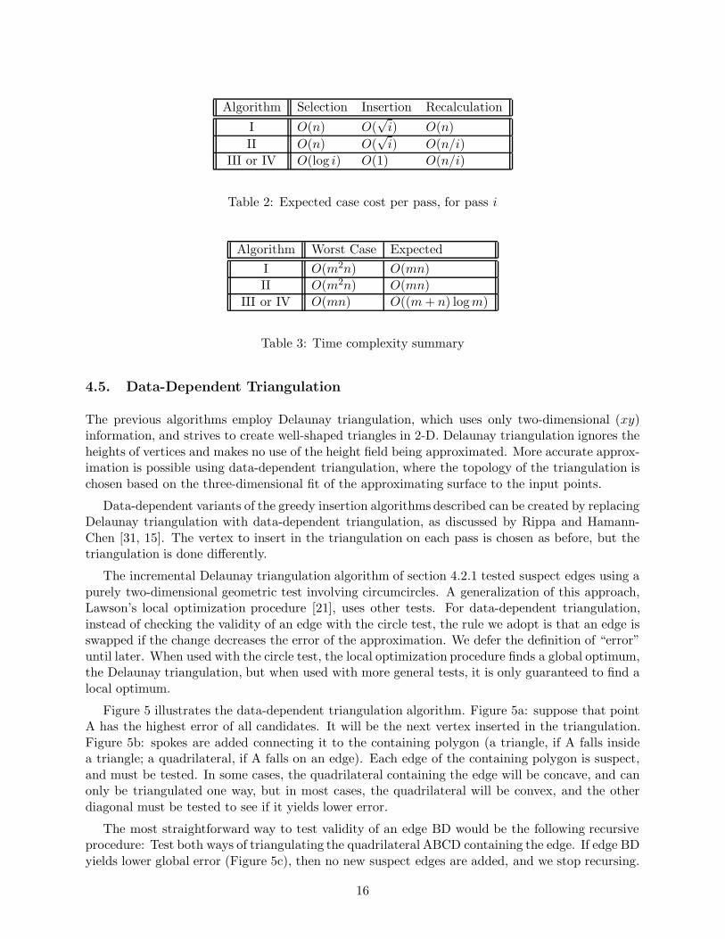
Cost Summary. The complexity figures for the three algorithms presented are summarized inTables 1, 2, and 3. Tables 1 and 2 detail the worst and expected costs per pass, respectively.Table 3 provides a summary of the total worst case and expected time complexity for each of thealgorithms.

15

Algorithm Selection Insertion Recalculation

I O(n) O(√i) O(n)

II O(n) O(√i) O(n/i)

III or IV O(log i) O(1) O(n/i)

Table 2: Expected case cost per pass, for pass i

Algorithm Worst Case ExpectedI O(m2n) O(mn)II O(m2n) O(mn)

III or IV O(mn) O((m+ n) logm)

Table 3: Time complexity summary

4.5. Data-Dependent Triangulation

The previous algorithms employ Delaunay triangulation, which uses only two-dimensional (xy)information, and strives to create well-shaped triangles in 2-D. Delaunay triangulation ignores theheights of vertices and makes no use of the height field being approximated. More accurate approx-imation is possible using data-dependent triangulation, where the topology of the triangulation ischosen based on the three-dimensional fit of the approximating surface to the input points.

Data-dependent variants of the greedy insertion algorithms described can be created by replacingDelaunay triangulation with data-dependent triangulation, as discussed by Rippa and Hamann-Chen [31, 15]. The vertex to insert in the triangulation on each pass is chosen as before, but thetriangulation is done differently.

The incremental Delaunay triangulation algorithm of section 4.2.1 tested suspect edges using apurely two-dimensional geometric test involving circumcircles. A generalization of this approach,Lawson’s local optimization procedure [21], uses other tests. For data-dependent triangulation,instead of checking the validity of an edge with the circle test, the rule we adopt is that an edge isswapped if the change decreases the error of the approximation. We defer the definition of “error”until later. When used with the circle test, the local optimization procedure finds a global optimum,the Delaunay triangulation, but when used with more general tests, it is only guaranteed to find alocal optimum.

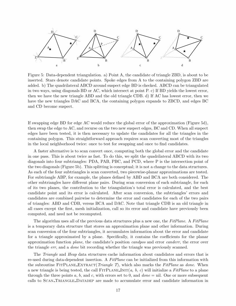
Figure 5 illustrates the data-dependent triangulation algorithm. Figure 5a: suppose that pointA has the highest error of all candidates. It will be the next vertex inserted in the triangulation.Figure 5b: spokes are added connecting it to the containing polygon (a triangle, if A falls insidea triangle; a quadrilateral, if A falls on an edge). Each edge of the containing polygon is suspect,and must be tested. In some cases, the quadrilateral containing the edge will be concave, and canonly be triangulated one way, but in most cases, the quadrilateral will be convex, and the otherdiagonal must be tested to see if it yields lower error.

The most straightforward way to test validity of an edge BD would be the following recursiveprocedure: Test both ways of triangulating the quadrilateral ABCD containing the edge. If edge BDyields lower global error (Figure 5c), then no new suspect edges are added, and we stop recursing.

16

★A

Z

D

AP

B

C

D

B

C

D

A

B

C

D

A

B

C

★

★

★

★

Z

a dcb

★

Z

Figure 5: Data-dependent triangulation. a) Point A, the candidate of triangle ZBD, is about to beinserted. Stars denote candidate points. Spoke edges from A to the containing polygon ZBD areadded. b) The quadrilateral ABCD around suspect edge BD is checked. ABCD can be triangulatedin two ways, using diagonals BD or AC, which intersect at point P. c) If BD yields the lowest error,then we have the new triangle ABD and the old triangle CDB. d) If AC has lowest error, then wehave the new triangles DAC and BCA, the containing polygon expands to ZBCD, and edges BCand CD become suspect.

If swapping edge BD for edge AC would reduce the global error of the approximation (Figure 5d),then swap the edge to AC, and recurse on the two new suspect edges, BC and CD. When all suspectedges have been tested, it is then necessary to update the candidates for all the triangles in thecontaining polygon. This straightforward approach requires scan converting most of the trianglesin the local neighborhood twice: once to test for swapping and once to find candidates.

A faster alternative is to scan convert once, computing both the global error and the candidatein one pass. This is about twice as fast. To do this, we split the quadrilateral ABCD with its twodiagonals into four subtriangles: PDA, PAB, PBC, and PCD, where P is the intersection point ofthe two diagonals (Figure 5b). This splitting is conceptual; it is not a change to the data structures.As each of the four subtriangles is scan converted, two piecewise-planar approximations are tested.For subtriangle ABP, for example, the planes defined by ABD and BCA are both considered. Theother subtriangles have different plane pairs. During scan conversion of each subtriangle, for eachof its two planes, the contribution to the triangulation’s total error is calculated, and the bestcandidate point and its error is calculated. After scan conversion, the subtriangles’ errors andcandidates are combined pairwise to determine the error and candidates for each of the two pairsof triangles: ABD and CDB, versus BCA and DAC. Note that triangle CDB is an old triangle inall cases except the first, mesh initialization, call so its error and candidate have previously beencomputed, and need not be recomputed.

The algorithm uses all of the previous data structures plus a new one, the FitPlane. A FitPlaneis a temporary data structure that stores an approximation plane and other information. Duringscan conversion of the four subtriangles, it accumulates information about the error and candidatefor a triangle approximated by a plane. Specifically, it contains the coefficients for the planarapproximation function plane, the candidate’s position candpos and error canderr, the error overthe triangle err, and a done bit recording whether the triangle was previously scanned.

The Triangle and Heap data structures cache information about candidates and errors that isre-used during data-dependent insertion. A FitPlane can be initialized from this information withthe subroutine FitPlane Extract(Triangle T), which also marks the FitPlane as done. Whena new triangle is being tested, the call FitPlane Init(a, b, c) will initialize a FitPlane to a planethrough the three points a, b, and c, with errors set to 0, and done = nil. One or more subsequentcalls to Scan Triangle Datadep are made to accumulate error and candidate information in

17

the FitPlane. If this approximation plane turns out to be the best one, the heap is updated andthe error and candidate information is saved for later use with a call to Set Candidate (listedbelow).

Other routines used below are Left Triangle and Right Triangle, which return the tri-angles to the left and the right of a directed edge, respectively. The keyword var marks call-by-reference parameters.

Algorithm IV: Data-Dependent Greedy Insertion:

Set Candidate(var Triangle T, FitPlane fit ):T.heapptr ←Heap Change(T.heapptr, fit.canderr, T)T.candpos ← fit.candposT.err ← fit.err

Scan Point(Point x, var FitPlane fit ):err ←|H(x)− Interpolate To Plane(x, fit.plane)|fit.err ←Error Accum(fit.err, err)if err > fit.err then

fit.canderr ← errfit.candpos ← x

Scan Triangle Datadep(Point p, Point q, Point r, var FitPlane u, var FitPlane v ):% Scan convert triangle pqr, updating error and candidate for planes u and v.% Plane u might be nonexistent or already done.forall points x inside triangle pqr do

if u 6= nil and not u.done thenScan Point(x, u)

Scan Point(x, v)

First Better( float q1, float q2, float e1, float e2 ):% Return true iff edge 1 yields better triangulation of a quadrilateral than edge 2,% according to shape and fit.% q1 and q2 are “shape quality”, and e1 and e2 are fit error of the corresponding triangulations.qratio ←Min(q1, q2) / Max(q1, q2)% Use shape if shape of one triangulation is much better than other, otherwise use fit.if qratio ≤ qthresh then

return (q1 ≥ q2) % shape criterionelse

return (e1 ≤ e2) % fit error criterion

18

Check Swap(DirectedEdge e, FitPlane abd ):% Checks edge e, swapping it if that reduces error, updating triangulation and heap.% Error and candidate for the triangle to the left of e is passed in in abd, if available.% Points a, b, c, d, and p are as shown in figure 5b, and e is edge from b to d.if abd = nil then

FitPlane abd ←FitPlane Init(a, b, d)if edge e is on perimeter of input grid or quadrilateral abcd is concave then

% Edge bd is good and edge ac is bad.if not abd.done then

Scan Triangle Datadep(a, b, d, nil, abd)Set Candidate(Left Triangle(e), abd)

else% Check whether diagonal bd or ac has lower error.FitPlane cdb ←FitPlane Extract(Right Triangle(e))FitPlane dac ←FitPlane Init(d, a, c)FitPlane bca ←FitPlane Init(b, c, a)Scan Triangle Datadep(p, d, a, abd, dac)% scan convert the four subtrianglesScan Triangle Datadep(p, a, b, abd, bca)Scan Triangle Datadep(p, b, c, cdb, bca)Scan Triangle Datadep(p, c, d, cdb, dac)ebd ←Error Combine(abd.err, cdb.err)eac ←Error Combine(dac.err, bca.err)if First Better(Shape Quality(a, b, c, d), Shape Quality(b, c, d, a), ebd, eac) then

% keep edge bdSet Candidate(Left Triangle(e), abd)if not cdb.done then

Set Candidate(Right Triangle(e), cdb)else

swap edge e from bd to acdac.done ← bca.done ← trueCheck Swap(DirectedEdge cd, dac)% recurseCheck Swap(DirectedEdge bc, bca)

Insert Datadep(Point a, Triangle T ):mark input point at a as usedin triangulation, add spoke edges connecting a to vertices of its containing polygon

(T and possibly a neighbor of T )forall counterclockwise perimeter edges e of containing polygon do

Check Swap(e, nil)

Greedy Insert Datadep():initialize mesh to two triangles with the height field corners as verticese := (either directed edge along diagonal of initial triangulation)Check Swap(e, nil)while not Goal Met() do

T ←Heap Delete Max()Insert Datadep(T.candpos, T)

The routines Error Accum and Error Combine are used to accumulate the error over asubtriangle, and to total the error of a pair of triangles, respectively. These can be defined invarious ways. For an L2 error measure, they should be defined:

19

float Error Accum(float accum, float x ):return accum+x ∗x

float Error Combine(float err1, float err2 ):return err1+err2

and for an L∞ error measure, they should be defined:

float Error Accum(float accum, float x ):return Max(accum, x)

float Error Combine(float err1, float err2 ):return Max(err1, err2)

4.5.1. Combating Slivers

Pure data-dependent triangulation, which makes swapping decisions based exclusively on fit error,will sometimes generate very thin sliver triangles. If the triangles fit the data well, and the surfaceis being displayed in shaded (not vector) form, then slivers by themselves are not a problem. Butsometimes these slivers do not fit the data well, and lead to globally inaccurate approximations.One approach which has been used to combat slivers is a hybrid of data-dependent and Delaunaytriangulation [31]. We wished to find a more elegant solution, however.

Our first hypothesis about the cause of the slivers was that narrow quadrilaterals containing fewor no input points were never having their diagonals swapped because of the boundary conditionsof the inequalities in our code (the case e1 = e2 = 0). With either the L2 or L∞ error normdescribed above, triangles containing no input points will have zero error. To address this situation,one can change the error formula to integrate the squared error between the piecewise planarapproximation and a bilinear interpolation of the height field grid, instead of simply summing onthe grid. This integrated error norm will yield nearly identical results for fat triangles, but it can bequite different for slivers. For a sliver triangle containing no input points, integration will penalizethose that deviate from the heights of the input points surrounding the middle of the triangle,while summation will not.

To our surprise, empirical tests disproved this hypothesis, however. When run on both syntheticand real DEM data, pure data-dependent triangulation using an integration error norm yielded nosignificant improvement over the same algorithm with a summation error norm; it was sometimesa bit better, and sometimes a bit worse. We therefore abandoned the idea of integration in theerror norm, and reluctantly adopted a hybrid algorithm.

The pseudocode above implements this hybrid. The procedure Shape Quality(a, b, c, d)returns a numerical rating of the shape of the triangles when quadrilateral abcd is split by edge bd.The parameter qthresh is a quality threshold. When set to 0, pure data-dependent triangulationresults, when set to 1, pure shape-dependent triangulation results, and when set in between, ahybrid results. If Shape Quality returns the minimum angle of the triangles abd and cdb, thenthis shape-dependent triangulation will in fact be Delaunay triangulation. The hybrid methodtended to yield the lowest error approximations overall.

4.5.2. Cost Analysis of Algorithm IV

In a greedy insertion algorithm, the data-dependent triangulation method described above is slowerthan Delaunay triangulation because it requires about twice as many error recalculations duringscan conversion. The asymptotic complexities are identical to algorithm III. Thus, algorithm IV’sworst case cost is O(mn) and its expected cost is O((m+n) logm).

20

x e1

e2e3

e4

e5

e6

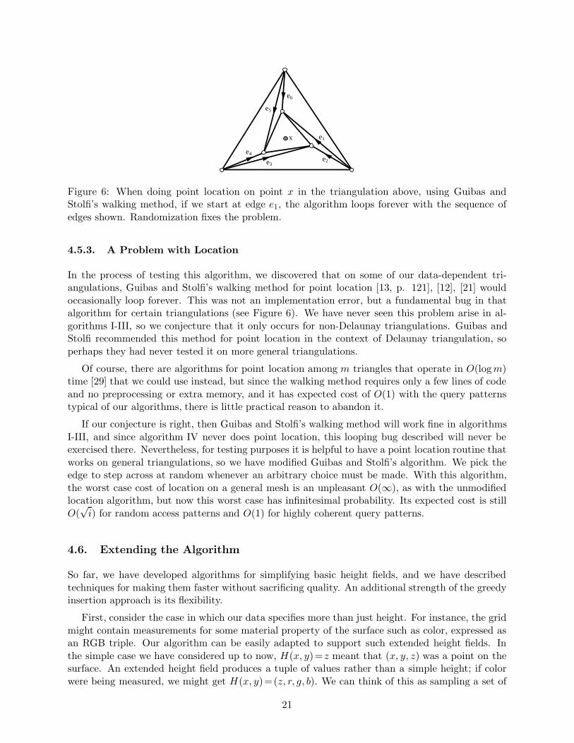
Figure 6: When doing point location on point x in the triangulation above, using Guibas andStolfi’s walking method, if we start at edge e1, the algorithm loops forever with the sequence ofedges shown. Randomization fixes the problem.

4.5.3. A Problem with Location

In the process of testing this algorithm, we discovered that on some of our data-dependent tri-angulations, Guibas and Stolfi’s walking method for point location [13, p. 121], [12], [21] wouldoccasionally loop forever. This was not an implementation error, but a fundamental bug in thatalgorithm for certain triangulations (see Figure 6). We have never seen this problem arise in al-gorithms I-III, so we conjecture that it only occurs for non-Delaunay triangulations. Guibas andStolfi recommended this method for point location in the context of Delaunay triangulation, soperhaps they had never tested it on more general triangulations.

Of course, there are algorithms for point location among m triangles that operate in O(logm)time [29] that we could use instead, but since the walking method requires only a few lines of codeand no preprocessing or extra memory, and it has expected cost of O(1) with the query patternstypical of our algorithms, there is little practical reason to abandon it.

If our conjecture is right, then Guibas and Stolfi’s walking method will work fine in algorithmsI-III, and since algorithm IV never does point location, this looping bug described will never beexercised there. Nevertheless, for testing purposes it is helpful to have a point location routine thatworks on general triangulations, so we have modified Guibas and Stolfi’s algorithm. We pick theedge to step across at random whenever an arbitrary choice must be made. With this algorithm,the worst case cost of location on a general mesh is an unpleasant O(∞), as with the unmodifiedlocation algorithm, but now this worst case has infinitesimal probability. Its expected cost is stillO(√i) for random access patterns and O(1) for highly coherent query patterns.

4.6. Extending the Algorithm

So far, we have developed algorithms for simplifying basic height fields, and we have describedtechniques for making them faster without sacrificing quality. An additional strength of the greedyinsertion approach is its flexibility.

First, consider the case in which our data specifies more than just height. For instance, the gridmight contain measurements for some material property of the surface such as color, expressed asan RGB triple. Our algorithm can be easily adapted to support such extended height fields. Inthe simple case we have considered up to now, H(x, y)=z meant that (x, y, z) was a point on thesurface. An extended height field produces a tuple of values rather than a simple height; if colorwere being measured, we might get H(x, y)=(z, r, g, b). We can think of this as sampling a set of

21

distinct surfaces, one in xyz-space, one in xyr-space, and so on. We see here another reason to rejecttriangulation schemes that attempt to fit specific surface characteristics; we now have 4 distinctsurfaces which need have no features in common. Given data for a generic set of surfaces, we canapply the importance measure to each surface separately and then compute some kind of averageof these values. But when we know the precise interpretation of the data (i.e. the values representheight and color), we can construct a more informed measure. Our old measure was simply |∆z|;the most obvious extension to deal with color is |∆z|+M

3 (|∆r|+|∆g|+|∆b|). Here, M is the z-rangeof H ; the M

3 term scales the total color difference to fit the range of the total height difference(here we assume that color values are between 0 and 1). In order to achieve greater flexibility, wecan also add a color emphasis parameter, w, controlling the relative importance of height differenceand color difference. The final error formula would be: (1− w)|∆z|+ wM

3 (|∆r|+ |∆g|+ |∆b|).To implement these changes, we simply added fields to the height field to record r, g, and

b, modified the FitPlane to retain planar approximations to these three additional surfaces, andchanged the error procedure to use the extended formula above.

These extensions allow our algorithm to be used to simplify terrains with color texture orplanar color images [35]. The output of such a simplification is a triangulated surface with linearinterpolation of color across each triangle. Such models are ideally suited for hardware-assistedGouraud shading [9] on most graphics workstations, and are a possible substitute for texturemapping when that is not supported by hardware.

5. Results

We have implemented all four algorithms above. Our combined implementation of algorithms IIIand IV consists of about 5,200 lines of C++. The incremental Delaunay triangulation module isadapted from Lischinski’s code [23].

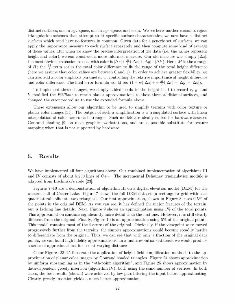
Figures 7–10 are a demonstration of algorithm III on a digital elevation model (DEM) for thewestern half of Crater Lake. Figure 7 shows the full DEM dataset (a rectangular grid with eachquadrilateral split into two triangles). Our first approximation, shown in Figure 8, uses 0.5% ofthe points in the original DEM. As you can see, it has defined the major features of the terrain,but is lacking fine details. Next, Figure 9 shows an approximation using 1% of the total points.This approximation contains significantly more detail than the first one. However, it is still clearlydifferent from the original. Finally, Figure 10 is an approximation using 5% of the original points.This model contains most of the features of the original. Obviously, if the viewpoint were movedprogressively further from the terrains, the simpler approximations would become steadily harderto differentiate from the original. Thus, we can see that with only a fraction of the original datapoints, we can build high fidelity approximations. In a multiresolution database, we would producea series of approximations, for use at varying distances.

Color Figures 23–25 illustrate the application of height field simplification methods to the ap-proximation of planar color images by Gouraud shaded triangles. Figure 24 shows approximationby uniform subsampling as in the “nth-point algorithm”, and Figure 25 shows approximation bydata-dependent greedy insertion (algorithm IV), both using the same number of vertices. In bothcases, the best results (shown) were achieved by low pass filtering the input before approximating.Clearly, greedy insertion yields a much better approximation.

22

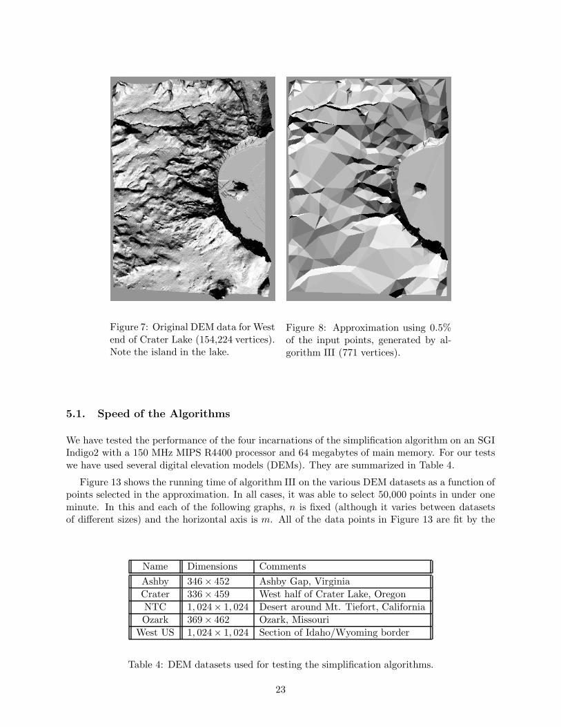
Figure 7: Original DEM data for Westend of Crater Lake (154,224 vertices).Note the island in the lake.

Figure 8: Approximation using 0.5%of the input points, generated by al-gorithm III (771 vertices).

5.1. Speed of the Algorithms

We have tested the performance of the four incarnations of the simplification algorithm on an SGIIndigo2 with a 150 MHz MIPS R4400 processor and 64 megabytes of main memory. For our testswe have used several digital elevation models (DEMs). They are summarized in Table 4.

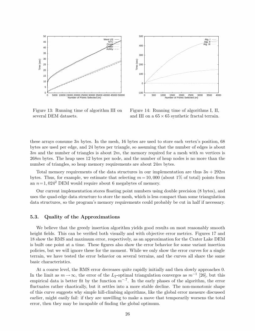
Figure 13 shows the running time of algorithm III on the various DEM datasets as a function ofpoints selected in the approximation. In all cases, it was able to select 50,000 points in under oneminute. In this and each of the following graphs, n is fixed (although it varies between datasetsof different sizes) and the horizontal axis is m. All of the data points in Figure 13 are fit by the

Name Dimensions CommentsAshby 346× 452 Ashby Gap, VirginiaCrater 336× 459 West half of Crater Lake, OregonNTC 1, 024× 1, 024 Desert around Mt. Tiefort, CaliforniaOzark 369× 462 Ozark, Missouri

West US 1, 024× 1, 024 Section of Idaho/Wyoming border

Table 4: DEM datasets used for testing the simplification algorithms.

23

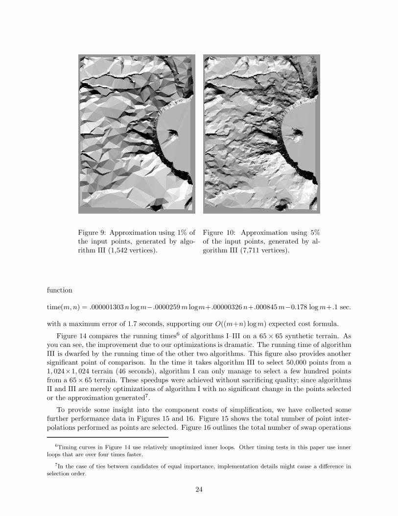
Figure 9: Approximation using 1% ofthe input points, generated by algo-rithm III (1,542 vertices).

Figure 10: Approximation using 5%of the input points, generated by al-gorithm III (7,711 vertices).

function

time(m, n) = .000001303n logm−.0000259m logm+.00000326 n+.000845m−0.178 logm+.1 sec.

with a maximum error of 1.7 seconds, supporting our O((m+n) logm) expected cost formula.

Figure 14 compares the running times6 of algorithms I–III on a 65× 65 synthetic terrain. Asyou can see, the improvement due to our optimizations is dramatic. The running time of algorithmIII is dwarfed by the running time of the other two algorithms. This figure also provides anothersignificant point of comparison. In the time it takes algorithm III to select 50,000 points from a1, 024×1, 024 terrain (46 seconds), algorithm I can only manage to select a few hundred pointsfrom a 65× 65 terrain. These speedups were achieved without sacrificing quality; since algorithmsII and III are merely optimizations of algorithm I with no significant change in the points selectedor the approximation generated7.

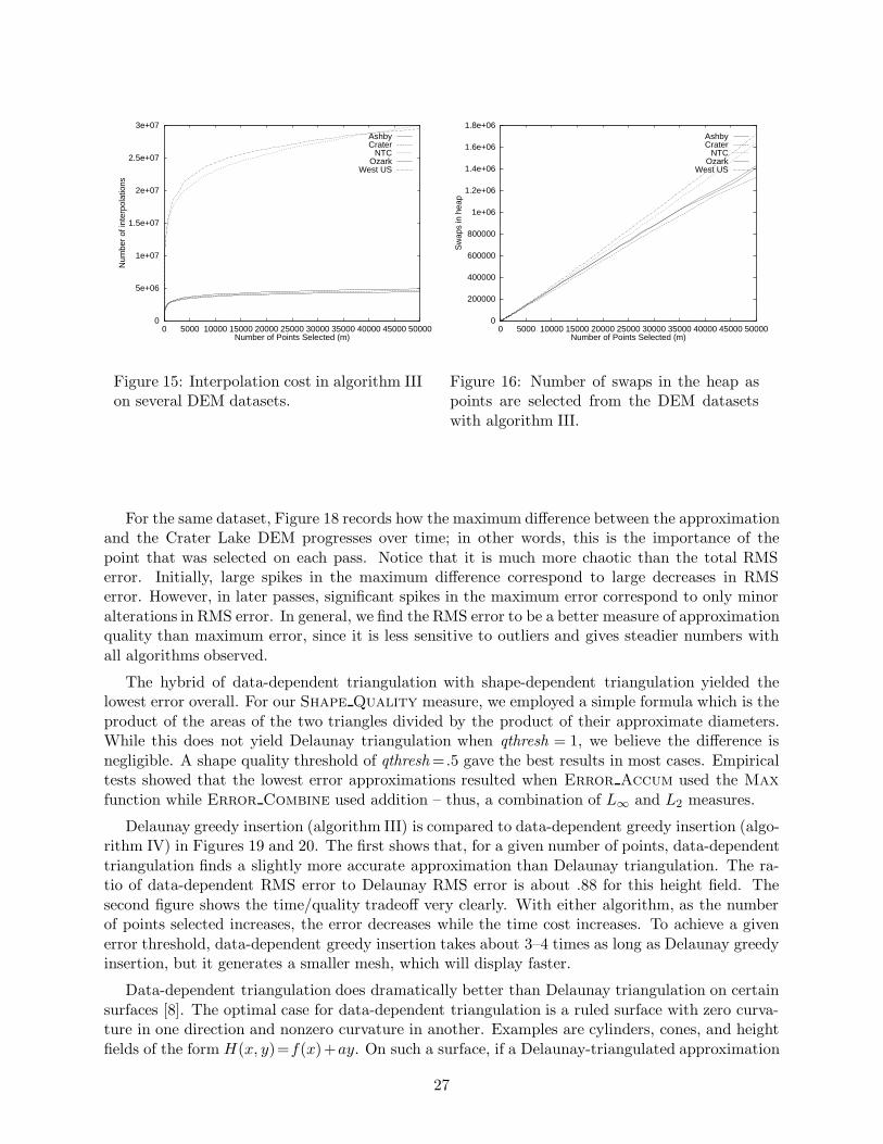
To provide some insight into the component costs of simplification, we have collected somefurther performance data in Figures 15 and 16. Figure 15 shows the total number of point inter-polations performed as points are selected. Figure 16 outlines the total number of swap operations

6Timing curves in Figure 14 use relatively unoptimized inner loops. Other timing tests in this paper use innerloops that are over four times faster.

7In the case of ties between candidates of equal importance, implementation details might cause a difference inselection order.

24

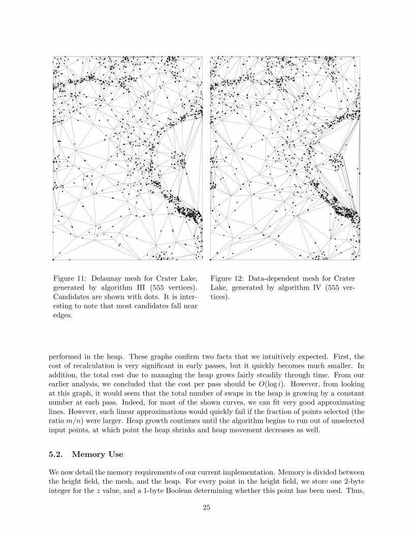
Figure 11: Delaunay mesh for Crater Lake,generated by algorithm III (555 vertices).Candidates are shown with dots. It is inter-esting to note that most candidates fall nearedges.

Figure 12: Data-dependent mesh for CraterLake, generated by algorithm IV (555 ver-tices).

performed in the heap. These graphs confirm two facts that we intuitively expected. First, thecost of recalculation is very significant in early passes, but it quickly becomes much smaller. Inaddition, the total cost due to managing the heap grows fairly steadily through time. From ourearlier analysis, we concluded that the cost per pass should be O(log i). However, from lookingat this graph, it would seem that the total number of swaps in the heap is growing by a constantnumber at each pass. Indeed, for most of the shown curves, we can fit very good approximatinglines. However, such linear approximations would quickly fail if the fraction of points selected (theratio m/n) were larger. Heap growth continues until the algorithm begins to run out of unselectedinput points, at which point the heap shrinks and heap movement decreases as well.

5.2. Memory Use

We now detail the memory requirements of our current implementation. Memory is divided betweenthe height field, the mesh, and the heap. For every point in the height field, we store one 2-byteinteger for the z value, and a 1-byte Boolean determining whether this point has been used. Thus,

25

0

5

10

15

20

25

30

35

40

45

50

0 5000 10000 15000 20000 25000 30000 35000 40000 45000 50000

Tim

e (s

ec)

Number of Points Selected (m)

West USNTC

OzarkCraterAshby

-100

0

100

200

300

400

500

0 500 1000 1500 2000 2500 3000 3500 4000

Tim

e (s

ec)

Number of Points Selected (m)

Alg. IAlg. II

Alg. III

Figure 13: Running time of algorithm III onseveral DEM datasets.

Figure 14: Running time of algorithms I, II,and III on a 65× 65 synthetic fractal terrain.

these arrays consume 3n bytes. In the mesh, 16 bytes are used to store each vertex’s position, 68bytes are used per edge, and 24 bytes per triangle, so assuming that the number of edges is about3m and the number of triangles is about 2m, the memory required for a mesh with m vertices is268m bytes. The heap uses 12 bytes per node, and the number of heap nodes is no more than thenumber of triangles, so heap memory requirements are about 24m bytes.

Total memory requirements of the data structures in our implementation are thus 3n + 292mbytes. Thus, for example, we estimate that selecting m= 10, 000 (about 1% of total) points froman n=1, 0242 DEM would require about 6 megabytes of memory.

Our current implementation stores floating point numbers using double precision (8 bytes), anduses the quad-edge data structure to store the mesh, which is less compact than some triangulationdata structures, so the program’s memory requirements could probably be cut in half if necessary.

5.3. Quality of the Approximations

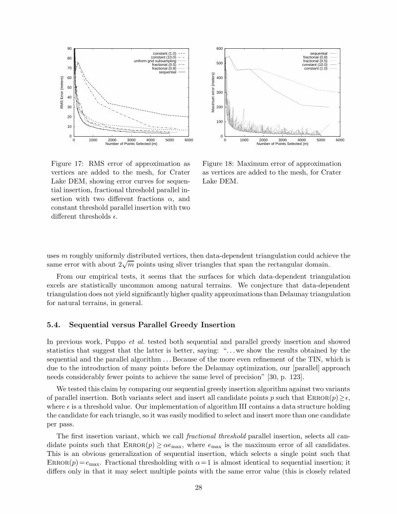
We believe that the greedy insertion algorithm yields good results on most reasonably smoothheight fields. This can be verified both visually and with objective error metrics. Figures 17 and18 show the RMS and maximum error, respectively, as an approximation for the Crater Lake DEMis built one point at a time. These figures also show the error behavior for some variant insertionpolicies, but we will ignore these for the moment. While we only show the error curves for a singleterrain, we have tested the error behavior on several terrains, and the curves all share the samebasic characteristics.

At a coarse level, the RMS error decreases quite rapidly initially and then slowly approaches 0.In the limit as m→∞, the error of the L2-optimal triangulation converges as m−1 [26], but thisempirical data is better fit by the function m−.7. In the early phases of the algorithm, the errorfluctuates rather chaotically, but it settles into a more stable decline. The non-monotonic shapeof this curve suggests why simple hill-climbing algorithms, like the global error measure discussedearlier, might easily fail: if they are unwilling to make a move that temporarily worsens the totalerror, then they may be incapable of finding the global optimum.

26

0

5e+06

1e+07

1.5e+07

2e+07

2.5e+07

3e+07

0 5000 10000 15000 20000 25000 30000 35000 40000 45000 50000

Num

ber

of in

terp

olat

ions

Number of Points Selected (m)

AshbyCrater

NTCOzark

West US

0

200000

400000

600000

800000

1e+06

1.2e+06

1.4e+06

1.6e+06

1.8e+06

0 5000 10000 15000 20000 25000 30000 35000 40000 45000 50000

Sw

aps

in h

eap

Number of Points Selected (m)

AshbyCrater

NTCOzark

West US

Figure 15: Interpolation cost in algorithm IIIon several DEM datasets.

Figure 16: Number of swaps in the heap aspoints are selected from the DEM datasetswith algorithm III.

For the same dataset, Figure 18 records how the maximum difference between the approximationand the Crater Lake DEM progresses over time; in other words, this is the importance of thepoint that was selected on each pass. Notice that it is much more chaotic than the total RMSerror. Initially, large spikes in the maximum difference correspond to large decreases in RMSerror. However, in later passes, significant spikes in the maximum error correspond to only minoralterations in RMS error. In general, we find the RMS error to be a better measure of approximationquality than maximum error, since it is less sensitive to outliers and gives steadier numbers withall algorithms observed.

The hybrid of data-dependent triangulation with shape-dependent triangulation yielded thelowest error overall. For our Shape Quality measure, we employed a simple formula which is theproduct of the areas of the two triangles divided by the product of their approximate diameters.While this does not yield Delaunay triangulation when qthresh = 1, we believe the difference isnegligible. A shape quality threshold of qthresh = .5 gave the best results in most cases. Empiricaltests showed that the lowest error approximations resulted when Error Accum used the Max

function while Error Combine used addition – thus, a combination of L∞ and L2 measures.

Delaunay greedy insertion (algorithm III) is compared to data-dependent greedy insertion (algo-rithm IV) in Figures 19 and 20. The first shows that, for a given number of points, data-dependenttriangulation finds a slightly more accurate approximation than Delaunay triangulation. The ra-tio of data-dependent RMS error to Delaunay RMS error is about .88 for this height field. Thesecond figure shows the time/quality tradeoff very clearly. With either algorithm, as the numberof points selected increases, the error decreases while the time cost increases. To achieve a givenerror threshold, data-dependent greedy insertion takes about 3–4 times as long as Delaunay greedyinsertion, but it generates a smaller mesh, which will display faster.

Data-dependent triangulation does dramatically better than Delaunay triangulation on certainsurfaces [8]. The optimal case for data-dependent triangulation is a ruled surface with zero curva-ture in one direction and nonzero curvature in another. Examples are cylinders, cones, and heightfields of the form H(x, y)=f(x)+ay. On such a surface, if a Delaunay-triangulated approximation

27

0

10

20

30

40

50

60

70

80

90

0 1000 2000 3000 4000 5000 6000

RM

S E

rror

(m

eter

s)

Number of Points Selected (m)

constant (1.0)constant (10.0)

uniform grid subsamplingfractional (0.5)fractional (0.8)

sequential

0

100

200

300

400

500

600

0 1000 2000 3000 4000 5000 6000

Max

imum

err

or (

met

ers)

Number of Points Selected (m)

sequentialfractional (0.8)fractional (0.5)

constant (10.0)constant (1.0)

Figure 17: RMS error of approximation asvertices are added to the mesh, for CraterLake DEM, showing error curves for sequen-tial insertion, fractional threshold parallel in-sertion with two different fractions α, andconstant threshold parallel insertion with twodifferent thresholds ε.

Figure 18: Maximum error of approximationas vertices are added to the mesh, for CraterLake DEM.

uses m roughly uniformly distributed vertices, then data-dependent triangulation could achieve thesame error with about 2

√m points using sliver triangles that span the rectangular domain.

From our empirical tests, it seems that the surfaces for which data-dependent triangulationexcels are statistically uncommon among natural terrains. We conjecture that data-dependenttriangulation does not yield significantly higher quality approximations than Delaunay triangulationfor natural terrains, in general.

5.4. Sequential versus Parallel Greedy Insertion

In previous work, Puppo et al. tested both sequential and parallel greedy insertion and showedstatistics that suggest that the latter is better, saying: “. . .we show the results obtained by thesequential and the parallel algorithm . . .Because of the more even refinement of the TIN, which isdue to the introduction of many points before the Delaunay optimization, our [parallel] approachneeds considerably fewer points to achieve the same level of precision” [30, p. 123].

We tested this claim by comparing our sequential greedy insertion algorithm against two variantsof parallel insertion. Both variants select and insert all candidate points p such that Error(p)≥ε,where ε is a threshold value. Our implementation of algorithm III contains a data structure holdingthe candidate for each triangle, so it was easily modified to select and insert more than one candidateper pass.

The first insertion variant, which we call fractional threshold parallel insertion, selects all can-didate points such that Error(p)≥ αemax, where emax is the maximum error of all candidates.This is an obvious generalization of sequential insertion, which selects a single point such thatError(p)=emax. Fractional thresholding with α=1 is almost identical to sequential insertion; itdiffers only in that it may select multiple points with the same error value (this is closely related

28

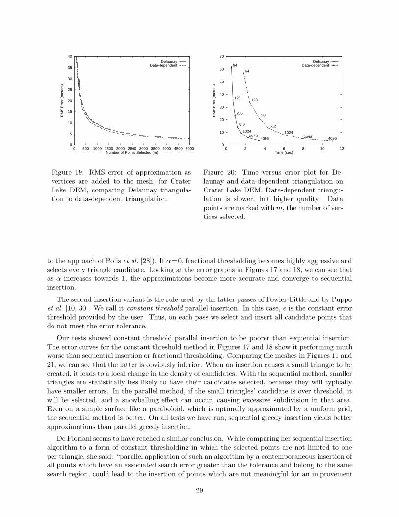
0

5

10

15

20

25

30

35

40

0 500 1000 1500 2000 2500 3000 3500 4000 4500 5000

RM

S E

rror

(m

eter

s)

Number of Points Selected (m)

DelaunayData-dependent

0

10

20

30

40

50

60

70

0 2 4 6 8 10 12

RM

S E

rror

(m

eter

s)

Time (sec)

64

128

256

512

10242048

4096

64

128

256

512

10242048 4096

DelaunayData-dependent

Figure 19: RMS error of approximation asvertices are added to the mesh, for CraterLake DEM, comparing Delaunay triangula-tion to data-dependent triangulation.

Figure 20: Time versus error plot for De-launay and data-dependent triangulation onCrater Lake DEM. Data-dependent triangu-lation is slower, but higher quality. Datapoints are marked with m, the number of ver-tices selected.

to the approach of Polis et al. [28]). If α=0, fractional thresholding becomes highly aggressive andselects every triangle candidate. Looking at the error graphs in Figures 17 and 18, we can see thatas α increases towards 1, the approximations become more accurate and converge to sequentialinsertion.

The second insertion variant is the rule used by the latter passes of Fowler-Little and by Puppoet al. [10, 30]. We call it constant threshold parallel insertion. In this case, ε is the constant errorthreshold provided by the user. Thus, on each pass we select and insert all candidate points thatdo not meet the error tolerance.

Our tests showed constant threshold parallel insertion to be poorer than sequential insertion.The error curves for the constant threshold method in Figures 17 and 18 show it performing muchworse than sequential insertion or fractional thresholding. Comparing the meshes in Figures 11 and21, we can see that the latter is obviously inferior. When an insertion causes a small triangle to becreated, it leads to a local change in the density of candidates. With the sequential method, smallertriangles are statistically less likely to have their candidates selected, because they will typicallyhave smaller errors. In the parallel method, if the small triangles’ candidate is over threshold, itwill be selected, and a snowballing effect can occur, causing excessive subdivision in that area.Even on a simple surface like a paraboloid, which is optimally approximated by a uniform grid,the sequential method is better. On all tests we have run, sequential greedy insertion yields betterapproximations than parallel greedy insertion.

De Floriani seems to have reached a similar conclusion. While comparing her sequential insertionalgorithm to a form of constant thresholding in which the selected points are not limited to oneper triangle, she said: “parallel application of such an algorithm by a contemporaneous insertion ofall points which have an associated search error greater than the tolerance and belong to the samesearch region, could lead to the insertion of points which are not meaningful for an improvement

29

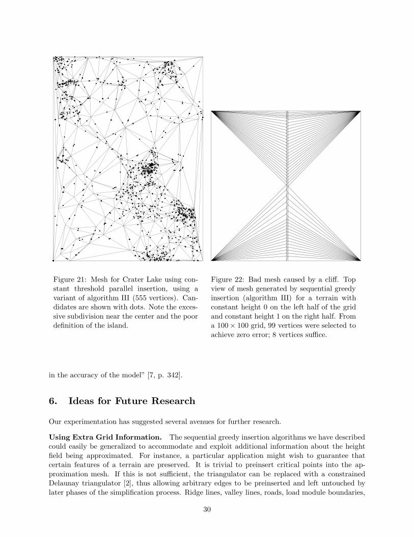
Figure 21: Mesh for Crater Lake using con-stant threshold parallel insertion, using avariant of algorithm III (555 vertices). Can-didates are shown with dots. Note the exces-sive subdivision near the center and the poordefinition of the island.

Figure 22: Bad mesh caused by a cliff. Topview of mesh generated by sequential greedyinsertion (algorithm III) for a terrain withconstant height 0 on the left half of the gridand constant height 1 on the right half. Froma 100× 100 grid, 99 vertices were selected toachieve zero error; 8 vertices suffice.

in the accuracy of the model” [7, p. 342].

6. Ideas for Future Research

Our experimentation has suggested several avenues for further research.

Using Extra Grid Information. The sequential greedy insertion algorithms we have describedcould easily be generalized to accommodate and exploit additional information about the heightfield being approximated. For instance, a particular application might wish to guarantee thatcertain features of a terrain are preserved. It is trivial to preinsert critical points into the ap-proximation mesh. If this is not sufficient, the triangulator can be replaced with a constrainedDelaunay triangulator [2], thus allowing arbitrary edges to be preinserted and left untouched bylater phases of the simplification process. Ridge lines, valley lines, roads, load module boundaries,

30

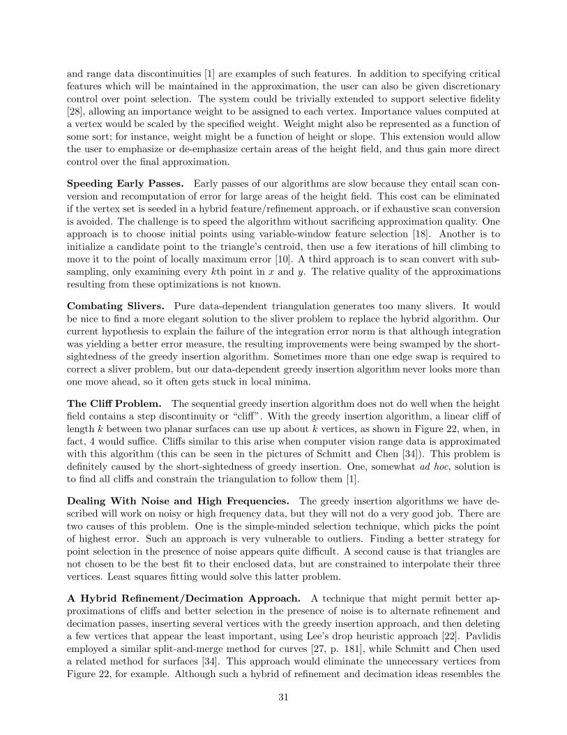
and range data discontinuities [1] are examples of such features. In addition to specifying criticalfeatures which will be maintained in the approximation, the user can also be given discretionarycontrol over point selection. The system could be trivially extended to support selective fidelity[28], allowing an importance weight to be assigned to each vertex. Importance values computed ata vertex would be scaled by the specified weight. Weight might also be represented as a function ofsome sort; for instance, weight might be a function of height or slope. This extension would allowthe user to emphasize or de-emphasize certain areas of the height field, and thus gain more directcontrol over the final approximation.

Speeding Early Passes. Early passes of our algorithms are slow because they entail scan con-version and recomputation of error for large areas of the height field. This cost can be eliminatedif the vertex set is seeded in a hybrid feature/refinement approach, or if exhaustive scan conversionis avoided. The challenge is to speed the algorithm without sacrificing approximation quality. Oneapproach is to choose initial points using variable-window feature selection [18]. Another is toinitialize a candidate point to the triangle’s centroid, then use a few iterations of hill climbing tomove it to the point of locally maximum error [10]. A third approach is to scan convert with sub-sampling, only examining every kth point in x and y. The relative quality of the approximationsresulting from these optimizations is not known.

Combating Slivers. Pure data-dependent triangulation generates too many slivers. It wouldbe nice to find a more elegant solution to the sliver problem to replace the hybrid algorithm. Ourcurrent hypothesis to explain the failure of the integration error norm is that although integrationwas yielding a better error measure, the resulting improvements were being swamped by the short-sightedness of the greedy insertion algorithm. Sometimes more than one edge swap is required tocorrect a sliver problem, but our data-dependent greedy insertion algorithm never looks more thanone move ahead, so it often gets stuck in local minima.

The Cliff Problem. The sequential greedy insertion algorithm does not do well when the heightfield contains a step discontinuity or “cliff”. With the greedy insertion algorithm, a linear cliff oflength k between two planar surfaces can use up about k vertices, as shown in Figure 22, when, infact, 4 would suffice. Cliffs similar to this arise when computer vision range data is approximatedwith this algorithm (this can be seen in the pictures of Schmitt and Chen [34]). This problem isdefinitely caused by the short-sightedness of greedy insertion. One, somewhat ad hoc, solution isto find all cliffs and constrain the triangulation to follow them [1].

Dealing With Noise and High Frequencies. The greedy insertion algorithms we have de-scribed will work on noisy or high frequency data, but they will not do a very good job. There aretwo causes of this problem. One is the simple-minded selection technique, which picks the pointof highest error. Such an approach is very vulnerable to outliers. Finding a better strategy forpoint selection in the presence of noise appears quite difficult. A second cause is that triangles arenot chosen to be the best fit to their enclosed data, but are constrained to interpolate their threevertices. Least squares fitting would solve this latter problem.

A Hybrid Refinement/Decimation Approach. A technique that might permit better ap-proximations of cliffs and better selection in the presence of noise is to alternate refinement anddecimation passes, inserting several vertices with the greedy insertion approach, and then deletinga few vertices that appear the least important, using Lee’s drop heuristic approach [22]. Pavlidisemployed a similar split-and-merge method for curves [27, p. 181], while Schmitt and Chen useda related method for surfaces [34]. This approach would eliminate the unnecessary vertices fromFigure 22, for example. Although such a hybrid of refinement and decimation ideas resembles the

31

algorithm of Hoppe et al. [19], it should be quite a bit faster since we already know how to do manyof the steps quickly.

If the least squares approach is taken further, allowing the vertex positions to drift in x andy, as well as z, this would provide an additional mechanism by which the algorithm could correctsub-optimal selections caused by noise or high frequency detail in the height field.

Generalization to Other Geometries. The algorithms presented here could easily be gener-alized from height field grids to scattered data approximation. That is, the xy projection of theinput points need not form a rectangular grid, but could be any finite point set. This change wouldrequire each triangle to store a set of points [6, 18, 11]. During re-triangulation, these sets wouldbe merged and split. Instead of scan converting a triangle, one would visit all the points in thattriangle’s point set.

Generalization of these techniques from piecewise-planar approximations of functions of twovariables to curved surface approximations and higher dimensional spaces [15] is fairly straightfor-ward.

Multiresolution Modeling. Further work is needed to build on the algorithms described hereto create multiresolution databases for fast terrain rendering. Such a system would need to supportdivision of a huge terrain into blocks, precomputation of multiple levels of detail, adaptive selectionof level of detail during display, and blending between levels of detail. Much of this work hasalready been done by others [28, 20].

Applications in Computer Vision. Finally, these algorithms can be used for the simplificationof range data in computer vision. The output data of many stereo and laser range scanners is inthe form of a height field or z-buffer in a perspective space, so it can be fed into the algorithmsdescribed here with little or no modification. When the triangles output by the algorithms areperspective-transformed to world space, their planarity is preserved, so the approximation in thatspace is also valid.

Some range scanners acquire data in a cylindrical format, outputting radius as a function ofazimuth and height: r(θ, z). The algorithms here could be modified to generate triangulatedapproximation to these surfaces, but since the transform between cylindrical space and world spaceis not a perspective one, nonlinear interpolation would be needed for best results.

As a binary variant of the selective fidelity concept, range data points that are known to beinaccurate can be flagged before being fed into the simplification algorithm, and these pointscan easily be ignored during vertex selection and error calculation. Our present implementationsupports this option. Further work is needed to test the present algorithm’s sensitivity to noiseand cliffs, and to determine if modification is necessary to deal with these two issues.

7. Summary

In this work we have implemented, optimized, and analyzed the greedy insertion algorithm.

The greedy insertion algorithm is a fast, flexible method that produces high quality approxima-tions. It takes a height field as input and produces a triangulated mesh approximating that heightfield as output. The algorithm starts with a minimal approximation consisting of two triangles andrepeatedly inserts as a vertex in the triangulation the input point with the greatest approximationerror. The process is terminated either when a given number of vertices is reached, or when the

32

error drops below a given error tolerance.

Beginning with a very simple implementation of the greedy insertion algorithm, we optimizedit in two ways. First, we exploited the locality of mesh changes, and only recalculated the errorsat input points for which the approximation changed, and second, we used a heap to permit thepoint of highest error to be found more quickly. When approximating an n point grid using an mvertex triangulated mesh, these optimizations sped up the algorithm from an expected time cost ofO(mn) to O((m+n) logm). This speedup is significant in practice as well as theory. For example,we can approximate a 1024×1024 grid to high quality using 1% of its points in about 21 seconds ona 150 MHz processor. The memory requirements of the algorithm are O(m+ n). We were able toachieve high speeds and simplify large grids with standard workstations; we did not employ moreexpensive computers.

We explored several variants of the greedy insertion algorithm in search of the best method forselecting important vertices. The four importance measures examined were: local error, curvature,global error, and products of these. We also tested refinement algorithms, which successively buildup a triangulation, against decimation algorithms, which successively simplify it. Our empiricalcomparisons on curves showed that a multi-pass refinement algorithm utilizing the local errormeasure, namely, the sequential greedy insertion method, produced the highest quality results.

Delaunay and data-dependent triangulation methods were compared. The latter is capable ofhigher quality approximations because it chooses the triangulation based on quality of data fit, noton the shape of a triangle’s xy projection.

Data-dependent triangulation can be relatively fast. Had we used the straightforward algorithm,data-dependent triangulation would have been many times slower than Delaunay triangulation,since it would scan convert about twice as many input points, doing more work at each point, andit would visit each of these points twice, once for swap testing and once for candidate selection.We described a new, faster data-dependent triangulation algorithm that merges swap testing andcandidate selection into one pass, saving a factor of two in cost.

With our implementation, we found that data-dependent triangulation takes about 3–4 times aslong as Delaunay triangulation, and yields slightly higher quality on typical terrains. In applicationswhere simplification speed is critical, Delaunay triangulation would be preferred, but if the quality ofthe approximation is primary, and the height field will be rendered many times after simplification,then the simplification cost is less important, and the data-dependent method is recommended.

We were surprised that data-dependent triangulation did not work better on terrain, since itapproximates certain surfaces, such as ruled surfaces, much better than Delaunay triangulation.Perhaps this says something about the isotropy of curvature in natural terrains. Further work isneeded to investigate this.

The greedy insertion algorithm is quite flexible. It makes no assumptions that limit its usage toterrains; it is applicable to any height field. In addition, it is easily generalized to extended heightfields with material properties such as color. Indeed it can be trivially generalized to arbitrarydiscrete functions defined over a rectangular domain; examples include the approximation of colorraster images by a set of Gouraud shaded polygons, and approximating computer vision range datawith triangulated surfaces.

Compared to previous work, our Delaunay greedy insertion algorithm yields nearly identical ap-proximations to those of De Floriani et al., Rippa, and Franklin [7, 31, 11], but from the informationavailable, it appears that our algorithm is the fastest both in theory and in practice.

Part of Heller’s adaptive triangular mesh filtering technique is a greedy insertion algorithm

33

employing heaps and local recalculation. That portion of his algorithm appears nearly identical toours in quality and asymptotic complexity [18, p. 168]. Because the initial pass of his algorithmuses feature selection, we suspect, however, that his could be faster but that our method willproduce somewhat higher quality approximations.

We have tested our sequential greedy insertion algorithm against the parallel greedy insertionalgorithms of Fowler-Little and Puppo et al. [10, 30], and found that sequential greedy insertionyields superior approximations in all cases tested. It appears that the sequential method usesvertices more carefully and leads to less unnecessary subdivision in the mesh.

While the greedy insertion algorithm discussed here is quite fast, and for most terrains it gen-erates high quality approximations, it is far from perfect. It does poorly in the vicinity of cliffsand in the presence of high noise levels or high frequencies, generating approximations that are farfrom optimal in those cases. Several ideas for improving the algorithm have been proposed here.

Further empirical and theoretical comparisons between methods will be needed to reach a deeperunderstanding of the surface simplification problem.

Portable C++ code for our Delaunay and data-dependent greedy insertion algorithms (algo-rithms III and IV) is available by World Wide Web from http://www.cs.cmu.edu/˜garland/scapeor by anonymous FTP from ftp.cs.cmu.edu in /afs/cs/user/garland/public/scape.

8. Acknowledgements

We thank Michael Polis, Stephen Gifford, and Dave McKeown for exchanging algorithmic ideaswith us and for sharing DEM data, and Anoop Bhattacharjya and Jon Webb for their thoughtson the application of these techniques to computer vision range data. The CMU Engineering &Science library has been very helpful in locating obscure papers. This work was supported byARPA contract F19628-93-C-0171 and NSF Young Investigator award CCR-9357763.

9. References

[1] Xin Chen and Francis Schmitt. Adaptive range data approximation by constrained surface triangula-tion. In B. Falcidieno and T. Kunii, editors, Modeling in Computer Graphics: Methods and Applications,pages 95–113. Springer-Verlag, Berlin, 1993.

[2] L. Paul Chew. Constrained Delaunay triangulations. Algorithmica, 4:97–108, 1989.

[3] James H. Clark. Hierarchical geometric models for visible surface algorithms. CACM, 19(10):547–554,Oct. 1976.

[4] Thomas H. Cormen, Charles E. Leiserson, and Ronald L. Rivest. Introduction to Algorithms. MITPress, Cambridge, MA, 1990.

[5] Mark de Berg and Katrin Dobrindt. On levels of detail in terrains. In Proc. 11th Annual ACM Symp.on Computational Geometry, Vancouver, B.C., June 1995. Also available as Utrecht University techreport UU-CS-1995-12, URL=ftp://ftp.cs.ruu.nl/pub/RUU/CS/techreps/CS-1995/.

[6] Leila De Floriani. A pyramidal data structure for triangle-based surface description. IEEE ComputerGraphics and Applications, 9(2):67–78, March 1989.

[7] Leila De Floriani, Bianca Falcidieno, and Caterina Pienovi. A Delaunay-based method for surfaceapproximation. In Eurographics ’83, pages 333–350. Elsevier Science, 1983.

[8] Nira Dyn, David Levin, and Shmuel Rippa. Data dependent triangulations for piecewise linear inter-polation. IMA J. Numer. Anal., 10(1):137–154, Jan. 1990.

34

[9] James D. Foley, Andries van Dam, Steven K. Feiner, and John F. Hughes. Computer Graphics: Prin-ciples and Practice, 2nd ed. Addison-Wesley, Reading MA, 1990.

[10] Robert J. Fowler and James J. Little. Automatic extraction of irregular network digital terrain models.Computer Graphics (SIGGRAPH ’79 Proc.), 13(2):199–207, Aug. 1979.

[11] W. Randolph Franklin. tin.c, 1993. C code, URL=ftp://ftp.cs.rpi.edu/pub/franklin/tin.tar.gz.

[12] P. J. Green and R. Sibson. Computing Dirichlet tesselations in the plane. The Computer Journal,21(2):168–173, 1978.

[13] Leonidas Guibas and Jorge Stolfi. Primitives for the manipulation of general subdivisions and thecomputation of Voronoi diagrams. ACM Transactions on Graphics, 4(2):75–123, 1985.

[14] Leonidas J. Guibas, Donald E. Knuth, and Micha Sharir. Randomized incremental construction ofDelaunay and Voronoi diagrams. In Proc. 17th Intl. Colloq. — Automata, Languages, and Programming,volume 443 of Springer-Verlag LNCS, pages 414–431, Berlin, 1990. Springer-Verlag.

[15] Bernd Hamann and Jiann-Liang Chen. Data point selection for piecewise trilinear approximation.Computer-Aided Geometric Design, 11:477–489, 1994.

[16] Paul S. Heckbert and Michael Garland. Multiresolution modeling for fast rendering. In Proc. Graph-ics Interface ’94, pages 43–50, Banff, Canada, May 1994. Canadian Inf. Proc. Soc. URL=http://www.cs.cmu.edu/˜ph.

[17] Paul S. Heckbert and Michael Garland. Survey of surface approximation algorithms. Technical report,CS Dept., Carnegie Mellon U., 1995. CMU-CS-95-194, URL=http://www.cs.cmu.edu/˜garland/scape.

[18] Martin Heller. Triangulation algorithms for adaptive terrain modeling. In Proc. 4th Intl. Symp. onSpatial Data Handling, volume 1, pages 163–174, Zurich, 1990.

[19] Hugues Hoppe, Tony DeRose, Tom Duchamp, John McDonald, and Werner Stuetzle. Mesh optimiza-tion. In SIGGRAPH ’93 Proc., pages 19–26, Aug. 1993.

[20] Michael Jones. Lessons learned from visual simulation. In SIGGRAPH ’94 Course Notes CD-ROM,Course 14: Designing Real-Time Graphics for Entertainment, pages 39–71. ACM SIGGRAPH, July1994.

[21] Charles L. Lawson. Software for C1 surface interpolation. In John R. Rice, editor, MathematicalSoftware III, pages 161–194. Academic Press, NY, 1977. (Proc. of symp., Madison, WI, Mar. 1977).

[22] Jay Lee. A drop heuristic conversion method for extracting irregular network for digital elevationmodels. In GIS/LIS ’89 Proc., volume 1, pages 30–39. American Congress on Surveying and Mapping,Nov. 1989.

[23] Dani Lischinski. Incremental Delaunay triangulation. In Paul Heckbert, editor, Graphics Gems IV,pages 47–59. Academic Press, Boston, 1994.

[24] David Marr. Vision. Freeman, San Francisco, 1982.

[25] Donald E. McClure and S. C. Shwartz. A method of image representation based on bivariate splines.Technical report, Center for Intelligent Control Systems, MIT, Mar. 1989. CICS-P-113.

[26] Edmond Nadler. Piecewise linear best L2 approximation on triangulations. In C. K. Chui et al., editors,Approximation Theory V, pages 499–502, Boston, 1986. Academic Press.

[27] Theodosios Pavlidis. Structural Pattern Recognition. Springer-Verlag, Berlin, 1977.

[28] Michael F. Polis and David M. McKeown, Jr. Issues in iterative TIN generation to support large scalesimulations. In Proc. of Auto-Carto 11 (Eleventh Intl. Symp. on Computer-Assisted Cartography),pages 267–277, November 1993. URL=http://www.cs.cmu.edu/˜MAPSLab.

[29] Franco P. Preparata and Michael I. Shamos. Computational Geometry: an Introduction. Springer-Verlag, New York, NY, 1985.

35

[30] Enrico Puppo, Larry Davis, Daniel DeMenthon, and Y. Ansel Teng. Parallel terrain triangulation. Intl.J. of Geographical Information Systems, 8(2):105–128, 1994.

[31] Shmuel Rippa. Adaptive approximation by piecewise linear polynomials on triangulations of subsets ofscattered data. SIAM J. Sci. Stat. Comput., 13(5):1123–1141, Sept. 1992.

[32] Lori Scarlatos. Spatial Data Representations for Rapid Visualization and Analysis. PhD thesis, CSDept, State U. of New York at Stony Brook, 1993.

[33] Lori L. Scarlatos and Theo Pavlidis. Optimizing triangulations by curvature equalization. In Proc.Visualization ’92, pages 333–339. IEEE Comput. Soc. Press, 1992.

[34] Francis Schmitt and Xin Chen. Fast segmentation of range images into planar regions. In Conf. onComputer Vision and Pattern Recognition (CVPR ’91), pages 710–711. IEEE Comp. Soc. Press, June1991.

[35] David A. Southard. Piecewise planar surface models from sampled data. In N. M. Patrikalakis, editor,Scientific Visualization of Physical Phenomena, pages 667–680, Tokyo, 1991. Springer-Verlag.

[36] Michael Spivak. A Comprehensive Introduction to Differential Geometry. Publish or Perish, Inc., 1979.

[37] William Welch. Serious Putty: Topological Design for Variational Curves and Surfaces. PhD thesis,CS Dept, Carnegie Mellon U., 1995.

36

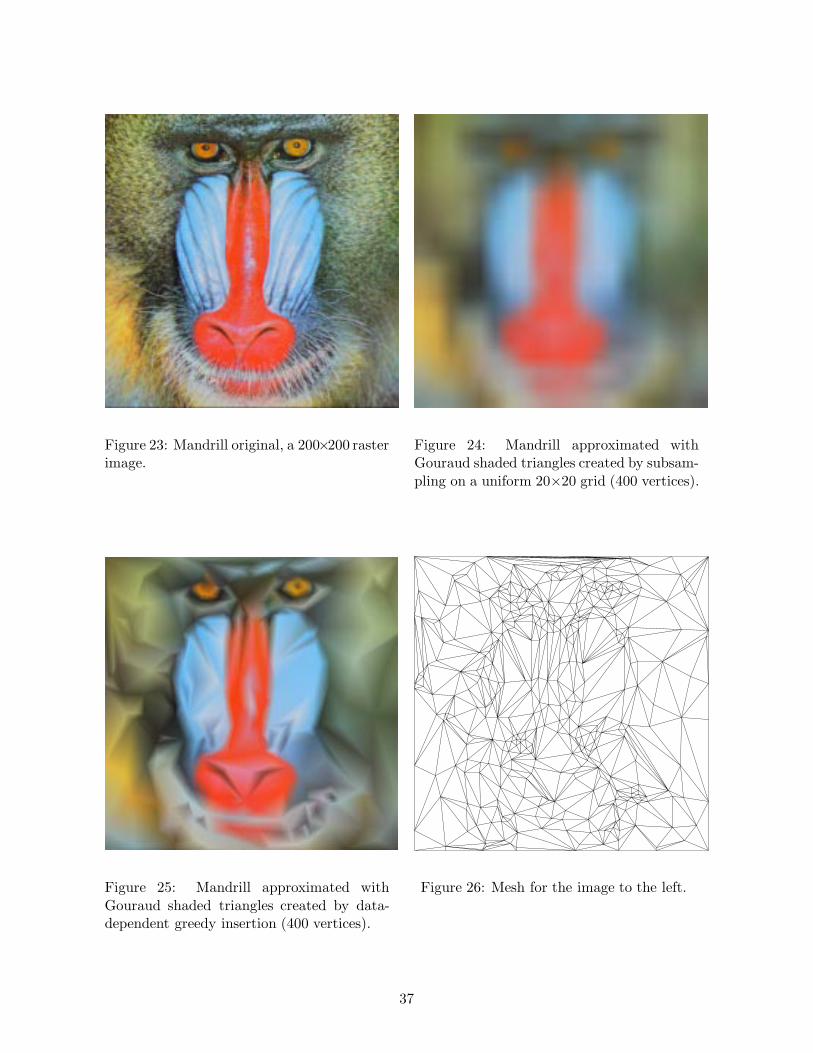
Figure 23: Mandrill original, a 200×200 rasterimage.

Figure 24: Mandrill approximated withGouraud shaded triangles created by subsam-pling on a uniform 20×20 grid (400 vertices).

Figure 25: Mandrill approximated withGouraud shaded triangles created by data-dependent greedy insertion (400 vertices).

Figure 26: Mesh for the image to the left.

37