Fast Object Localization and Pose Estimation inHeavy Clutter for Robotic Bin Picking

Ming-Yu Liu†∗ Oncel Tuzel† Ashok Veeraraghavan†‡

Yuichi Taguchi† Tim K. Marks† Rama Chellappa∗

†Mitsubishi Electric Research Laboratories (MERL)∗University of Maryland ‡Rice University

Abstract

We present a practical vision-based robotic bin-picking system that per-forms detection and 3D pose estimation of objects in an unstructured binusing a novel camera design, picks up parts from the bin, and performs er-ror detection and pose correction while the part is in the gripper. Two maininnovations enable our system to achieve real-time robust and accurate op-eration. First, we use a multi-flash camera that extracts robust depth edges.Second, we introduce an efficient shape-matching algorithmcalled fast di-rectional chamfer matching (FDCM), which is used to reliably detect objectsand estimate their poses. FDCM improves the accuracy of chamfer match-ing by including edge orientation. It also achieves massiveimprovements inmatching speed using line-segment approximations of edges, a 3D distancetransform, and directional integral images. We empirically show that thesespeedups, combined with the use of bounds in the spatial and hypothesisdomains, give the algorithm sublinear computational complexity. We alsoapply our FDCM method to other applications in the context ofdeformableand articulated shape matching. In addition to significantly improving uponthe accuracy of previous chamfer matching methods in all of the evaluatedapplications, FDCM is up to two orders of magnitude faster than the previousmethods.

1 Introduction

Building smarter, more flexible, and independent robots that can interact with thesurrounding environment is a fundamental goal of robotics research. Potential ap-plications are wide-ranging, including automated manufacturing, entertainment,

1

in-home assistance, and disaster rescue. One of the long-standing challenges in re-alizing this vision is the difficulty of “perception” and “cognition”—i.e., providingthe robot with the ability to understand its environment andmake inferences thatallow appropriate actions to be taken. Perception through inexpensive contact-freesensors such as cameras are essential for continuous and fast robot operation. Inthis paper, we address the challenge of robot perception in the context of industrialrobotics.

1.1 Visual Perception in Industrial Robotics

Computer vision has made rapid progress in the last decade, moving closer todefinitive solutions for longstanding problems in visual perception such as objectdetection [DT05, VJ01, TPM08], object recognition [FFFP06, OT01, DBdFF02],and pose estimation [AT06, SB06b, MREM04]. While the huge strides made inthese fields lead to important lessons, most of these methodscannot be readilyadapted to industrial robotics because many of the common assumptions are eitherviolated or invalid in such settings.

Material properties: One of the most common assumptions in traditional vi-sion algorithms relates to the characterization of the reflectance of materials in thescene. Most vision algorithms characterize materials as Lambertian [BJ03], i.e.,the appearance (radiance) of a single surface point is invariant to the location ofthe observer (camera). While this is a reasonable assumption in many scenarios,this is less applicable to industrial vision tasks. Severalcommon materials handledin industrial settings such as metal, glass, ceramics, and some plastics are not closeto Lambertian. Hence, using the Lambertian assumption for such objects generallyresults in poor performance. This necessitates industrialrobots to possess the abil-ity to understand and make inferences about objects that have complex reflectancecharacteristics.

Environmental challenges: The types of errors that afflict vision-based sys-tems in industrial settings are also very different from those in natural environ-ments. Several industrial assembly and manufacturing tasks must be accomplishedin dark or dimly lit environments with dust, dirt, grime, andgrease. It is essentialfor vision-based techniques to be able to cope with such sources of error in orderto be successful in such environments.

Variable appearance:The most popular methods for object detection, recog-nition, and pose estimation are based on the idea of feature descriptors such asScale Invariant Feature Transform (SIFT) [Low04], Histogram of Gradients (HOG)[DT05], and SURF [BETG08]. The basic idea is to detect several keypoint loca-tions on the surface of each object and compute these featuredescriptors at thesekeypoint locations. The features of each object are then stored in a database. Whena test image is acquired, the keypoint locations and the feature descriptors for the

2

test image are computed and then matched to the features stored in the database.An appropriately computed matching score is used to detect and recognize ob-jects, and the geometric relationship between the matched keypoint locations inthe test image and the database are used to make inferences about the poses ofthe objects. This general principle is quite popular and is used in several objectrecognition methods [STFW05, LSP06, NFF07]. Unfortunately, this successfulparadigm cannot be easily adapted to industrial robotics because visual appearancefeatures are unreliable in industrial settings. Variable material properties, as well asuncontrolled illumination and environmental conditions,make appearance-baseddescriptors unreliable and preclude the use of such techniques in most industrialapplications.

Background Clutter: The objects in a factory environment are usually stackedin part containers, which produces additional challenges such as overlapping parts,occlusions, cast shadows, and complex backgrounds. Therefore, most commercialvision systems assume that parts are separated in a kitting stage before operation.Machine vision systems that are capable of handling clutter, occlusions, and com-plex backgrounds would eliminate the need for kitting stages, thereby allowingsuch systems to handle a complex bin of parts.

Model-based estimation:While industrial settings are challenging because ofthe above-mentioned factors, they are also in some ways morestructured and allowopportunities to exploit this structure. For example, 3D CAD models of most ofthe industrial parts are readily available. Even if some of them are not, the factthat most industrial assembly lines repeatedly handle a finite set of discrete partsmany times (order of millions) makes CAD model acquisition cost-effective. The3D CAD models provide a reliable source of information, potentially overcomingthe challenging reflectance and environmental conditions.

1.2 A Practical Vision-Based Robotic Bin-Picking System

In this paper, we present a practical vision-based robotic bin-picking system thatovercomes the challenges described in Section 1.1. The system performs detec-tion and estimation of the 3D poses of objects that are stacked in a part container,picks up the parts from the container using an industrial robot arm, performs poseverification and refinement while the part is in the gripper, and inserts the pickedpart at a designated position. We have introduced two novel ideas that allow usto achieve reliable, fast, and accurate operation: (1) Novel imaging hardware thatprovides reliable geometric features regardless of the object’s material and surfacecharacteristics; (2) Fast, robust, and accurate 3D pose estimation based on the FastDirectional Chamfer Matching (FDCM) algorithm.

The fundamental challenges that arise due to non-Lambertian materials (e.g.,metal, glass, ceramic), textureless parts (e.g., uniformly painted parts), and greasy

3

and dirty environments lead to the fact that photometric features such as color andappearance descriptors are not robust enough in industrialsettings. This motivatesthe need to develop features that are dependent on the geometry of the part ratherthan its photometry. We use an inexpensive camera design, the multi-flash camera(MFC) [RTF+04], that provides reliable geometric features: depth edges. Thelocation of the depth edges on an object are dependent only onthe pose of the objectwith respect to the observer and the object geometry. Therefore, depth edges canbe used to determine the pose of the object uniquely. In addition, these geometricdescriptors allow easy and efficient incorporation of the 3DCAD models into oursystem. Given the 3D CAD model of an object, we retrieve the pose of the objectthat provides the best match between the observed features and the depth edgesfrom the CAD model. This allows us to bypass a time-consumingtraining phasefor each of the objects that would otherwise be necessary. A new part can beintegrated into our system in less than 10 minutes.

Although many shape matching algorithms have been proposedover the decades,chamfer matching (CM) [BTBW77] remains among the fastest and most robust ap-proaches in the presence of clutter. We adapt traditional chamfer matching with ahost of techniques to improve reliability, accuracy, and speed. First, we exploit thegeometric redundancies in the 3D structure of industrial parts by approximating theedge features using line segments. This, along with a 3D integral distance trans-form representation, allows us to both reduce the memory footprint and speed upthe matching algorithm by orders of magnitude. Second, we incorporate a direc-tional error term in the distance transform definition whichsignificantly improvesthe reliability, robustness, and accuracy of matching. Further, we improve the poseestimation accuracy using a continuous optimization procedure. The result is asystem that is capable of real-time operation for several industrial assembly appli-cations.

While the primary goal of this research is to develop a robustand reliable visionsystem for industrial robotics, the FDCM algorithm also achieves state-of-the-artperformance in shape matching. We present two additional application domainsthat benefit from FDCM: deformable object detection using a hand-drawn shape,and human pose estimation.

The paper is organized as follows. We briefly overview the related literaturein Section 2. We present the shape matching algorithm and itsoptimization inSection 3. Pose estimation and the robotic bin-picking system are described inSection 4. We report on our extensive experimental validation of the proposedsystem and compare it to the state of the art in Section 5. The paper is concludedin Section 6. We note that this paper builds upon our previouswork [LTV+10,LTVC10].

4

2 Related Work

In recent decades, there has been a considerable amount of work on automating theprocess of part assembly using vision systems [SI73, NPK96,ASBR10]. Thoughvision systems are successful in identifying, inspecting,and locating parts in care-fully engineered manufacturing settings, it remains a great challenge to extend theirapplicability to more general, unconstrained settings. Also, they often make use ofsimple geometric features such as lines, circles, or ellipses and their spatial orga-nization [Vis]. Changing a target object in the assembly process would requiresignificant manual adjustments or algorithmic modifications.

Model-based vision systemsexploit 3D CAD models of objects, along witheither acquired 2D images or range sensor data, for image interpretation. Suchmethods provide means for efficient detection, recognition, and pose estimation ofobjects in cluttered environments [Low87, Low91, SM92, JH99, BN10, DUNI10].Methods such as [Low87, Low91, DD92] rely on establishing correspondencesbetween 2D image features and points in the 3D models in orderto obtain an initialestimate of object pose. The estimate is later refined using iterative algorithms.These correspondences are, however, difficult to obtain reliably.

Since establishing 3D-to-2D correspondences using imagesis a hard task, sev-eral systems rely either directly or indirectly on 3D information. Such methodsgreatly simplify the correspondence problem at the cost of increased hardware re-quirements. The most common approach is the use of 3D range sensors eitherbased on structured light [SS03] or on time of flight [CSD+10]. This provides theability to establish 3D-to-3D point correspondences by matching 3D point descrip-tors from the CAD model to those in the acquired point cloud data. Several 3Dpoint descriptors [SM92, JH99, BN10] have been proposed formatching the 3Dscene points to the model points. To remove false matches, aninterpretation treeprocedure [GLP84] can be applied to find mutually consistentpairs. With theseconsistent pairs, one can use Horn’s method [Hor87] to estimate the object’s 3Dpose. Unfortunately, these descriptors are less reliable for pose estimation of indus-trial parts because these objects are mostly made of planar surfaces, which leads tovery few and uninformative features.

Recently, the use of the multi-flash camera [RTF+04] for object pose estima-tion was proposed in [ASBR10]. The MFC, which was originallydeveloped in thecontext of non-photorealistic rendering, provides depth edge features that can beused for pose estimation tasks. In this paper and in [LTV+10], we significantlyexpand the scope and impact of MFC for industrial robotics. While [ASBR10]presented a system capable of handling isolated parts, herewe present a systemthat can handle multitudes of parts randomly placed in a cluttered bin. Further, wealso present a novel shape-matching algorithm that resultsin better accuracy and

5

orders-of-magnitude improvement in matching speed, allowing real-time systemperformance.

One of the main technical contributions of this work is the development of thefast directional chamfer matching algorithm, which is widely applicable to severalapplications that currently use shape matching. Below, we briefly discuss relatedapproaches in shape matching.

Shape matchinghas been an active area in robotic vision research. Severalauthors have proposed shape representations and similarity measures that aim tobe invariant to object deformations [BMP02, LJ07]. These methods actively han-dle intra-class shape variations and achieve good performance in object recogni-tion. However, they require a clean segmentation of the target object. This ren-ders them less suitable for dealing with unstructured scenes due to the difficulty inforeground-background separation.

Recent studies focus on the recognition and localization ofobject shapes incluttered images. In [BBM05], the shape matching problem isposed as findingthe optimal correspondences between feature points, whichleads to an integerquadratic programming problem. In [FTG06], a contour segment network frame-work is proposed in which shape matching is formulated as finding paths on thenetwork that are similar to model outlines. In [FFJS08], Ferrari et al. proposea family of scale-invariant local shape descriptors (pair-of-adjacent-segment fea-tures) formed byk-connected nearly straight contour fragments in the edge map.These descriptors are later utilized in a shape matching framework [FJS10] througha voting scheme on a Hough space.

Zhu et al. [ZWWS08] formulate shape detection as a subset selection prob-lem on a set of salient contours. Due to the NP-hardness of theselection prob-lem, they compute an approximate solution using a two-stagelinear programmingprocedure. In [FS07], a hierarchical object contour representation is proposed tomodel shape variation, and the matching is performed using dynamic program-ming. In [RJM08], a multi-stage approach is employed in which coarse detections,which are established by matching subsets of contour segments, are pruned bybuilding the entire contour using dynamic programming.

These algorithms yield impressive results for matching shapes in cluttered im-ages. However, they share a common drawback, high computational complexity,which makes them unsuitable for time-critical applications. Although proposeddecades ago, chamfer matching [BTBW77] remains the preferred method whenspeed and accuracy are required, as discussed in [TSTC03]. In this paper, we pro-pose an improved version of chamfer matching and demonstrate its superiority withrespect to other variants [Gav98, SBC08]. Our approach improves the accuracy ofchamfer matching while greatly reducing its time complexity, leading to a speedupof up to two orders of magnitude in several application scenarios.

6

3 Fast Directional Chamfer Matching

In this section, we introduce ourfast directional chamfer matchingalgorithm,which we use for object detection and pose estimation in industrial robotics andother application areas.

3.1 Chamfer Matching

First we briefly explain standard chamfer matching (CM) [BTBW77], which is apopular technique for finding the best alignment between a template edge map anda query edge map. LetU = {ui}, wherei = 1, 2, ..., |U |, be the set of edge pixelsfrom a template edge map, and letV = {vj}, wherej = 1, 2, ..., |V |, be the set ofedge pixels from a query image edge map. Thechamfer distancebetweenU andV is defined as the average over all pixelsui ∈ U of the distance betweenui andits nearest pixel inV :

dCM(U, V ) =1

n

∑

ui∈U

minvj∈V

‖ui − vj‖. (1)

wheren is the number of template edge pixels,n = |U |.LetW be a warping function defined on the image plane that is parameterized

by s. For instance, ifW is a 2D Euclidean transformation, thens ∈ SE(2) can bewritten ass = (θ, tx, ty), wheretx and ty are translations parallel to thex andy axes, respectively, andθ is the in-plane rotation angle. Its action on each imagepointx ∈ R

2 is given via the transformation

W (x; s) =

(

cos(θ) − sin(θ)sin(θ) cos(θ)

)

x+

(

txty

)

. (2)

The best alignment parameters between the two edge maps is then given by

s = arg mins∈SE(2)

dCM(W (U ; s), V ) (3)

whereW (U ; s) = {W (ui, s)}, i = 1, 2, ..., |U |.The chamfer matching cost can be computed efficiently using the distance

transform imageDTV (x) = min

vj∈V‖x− vj‖, (4)

which specifies the distance from each pixelx in the distance transform image tothe nearest edge pixel inV . The distance transform can be computed in two passes

7

over the image using dynamic programming [FH04]. Using the distance transform,the cost function (1) can be evaluated in linear timeO(n) via

dCM(U, V ) =1

n

∑

ui∈U

DTV (ui). (5)

Chamfer matching provides a fairly smooth measure of fitnessand can toler-ate small rotations, misalignments, occlusions, and deformations. However, it be-comes less reliable in the presence of background clutter due to an increase in theproportion of false correspondences. To improve its robustness, several variants ofchamfer matching have been introduced that exploit edge orientation information.In [Gav98, DCS09], the template and query image edges are quantized into discreteorientation channels, and individual matching scores across channels are summed.Although these methods improve performance in cluttered scenes, the cost func-tion is sensitive to the number of orientation channels and becomes discontinuousacross channel boundaries. In [SBC08], the chamfer distance is augmented with anadditional cost for orientation mismatch, which is given bythe average differencein orientations between template edges and their nearest edge points in the queryimage. The method is known as oriented chamfer matching (OCM).

3.2 Directional Chamfer Matching

Instead of an explicit formulation of the orientation mismatch, we generalize thechamfer distance to points inR3 in order to match directional edge pixels. Eachedge pixelx is augmented with a direction term,φ(x), and the directional chamfermatching (DCM) score is given by

dDCM(U, V ) =1

n

∑

ui∈U

minvj∈V

(‖ui − vj‖+ λ‖φ(ui)− φ(vj)‖π) (6)

where the parameterλ is a weighting factor between the location and orientationterms. To compute the direction terms, we fit line segments tothe edge points (asexplained in Section 3.3), andφ(x) is the orientation of the line segment associatedwith point x. Note that the directions are written moduloπ: 0 ≤ φ(x) < π, andthe orientation error is defined as the minimum circular difference between the twodirections:

‖φ(x1)− φ(x2)‖π = min{

|φ(x1)− φ(x2)|,∣

∣ |φ(x1)− φ(x2)| − π∣

∣

}

. (7)

In Figure 1, we illustrate the differences between DCM and OCM [SBC08].The proposed matching cost, DCM, is a piecewise smooth function of both the

8

Template

edge point

Corresponding query

edge point

Template

edge point

Corresponding

query edge point

(a) (b)

Figure 1: Matching costs for an edge point. (a) Oriented chamfer matching(OCM) [SBC08]. (b) Directional chamfer matching (DCM, proposed in this pa-per). Whereas in OCM the location error is augmented with theorientation differ-ence from the nearest edge point, DCM jointly minimizes location and orientationerrors.

translation(tx, ty) and the rotation(θ) of the template pose. It is more robust toclutter, missing edges, and small misalignments.

The computational complexity of existing chamfer matchingalgorithms is lin-ear in the number of template edge points. Even though DCM includes an addi-tional direction term, our algorithm (derived in this section) computes theexactDCM score withsublinearcomplexity.

3.3 Line-Based Representation

The edge map of a scene is not an unstructured binary pattern.On the contrary, theobject contours comply with certain continuity constraints that can be retained bycombining line segments of various lengths, orientations,and translations. Basedon this observation, we represent an edge image as a collection ofm line segments.Compared with a set of points which has cardinalityn, its line-based representa-tion is more concise. Encoding an edge map using the line-based representationrequires onlyO(m) memory size, wherem << n, and is particularly suitablewhen the storage space for templates is limited. When the object exhibits a curvedcontour, more segments are required for good approximation, but the line-basedrepresentation is still more concise than the set of edge pixels.

We use a variant of the RANSAC [FB81] algorithm to compute theline-basedrepresentation of an edge map. The outline of the algorithm is as follows. Thealgorithm initially hypothesizes a variety of line segments by selecting a smallsubset of edge points and their directions. The support of each line segment isgiven by the set of points that satisfy the line’s equation upto a small residual,ν ≥ 0, and form a continuous structure. The line segment with the largest supportis retained, and its supporting points are removed from the set of edge points. The

9

(a) (b)

Figure 2: Line-based representation. (a) Edge image. The image contains 11,542edge points. (b) Line-based representation of the edge image. The image contains300 line segments.

procedure is repeated with the reduced set of edge points, until the support of thelongest line candidate becomes smaller than a few points.

The algorithm only retains edge points with continuity and sufficient support;therefore, the noise and isolated edges are filtered out. In addition, the directionsrecovered through the line fitting procedure are more precise than would be ob-tained using local operators such as image gradients. An example of the line-basedrepresentation is given in Figure 2, where a set of 11,542 points is modeled with300 line segments.

3.4 Three-Dimensional Distance Transform

The matching score given in (6) requires finding the minimum matching cost overlocation and orientation terms for each template edge point. Therefore, the com-putational complexity of the brute-force algorithm is quadratic in the number oftemplate and query image edge points. Here we present a three-dimensional dis-tance transform representation (DT3V ) for computing the matching cost in lineartime. A similar structure was also used in [OH97] for fast evaluation of Hausdorffdistances.

This representation is a three dimensional image tensor in which the first twodimensions are the locations in the image plane and the thirddimension belongs toa discrete set of edge orientations. We evenly quantize the edge orientation intoqdiscrete channels,Φ = {φi}, i = 1, 2, ..., q, which evenly divide the range[0 π).Each element of the tensor encodes the minimum distance to anedge point in thejoint location and orientation space:

DT3V (x, φ(x)) = minvj∈V

(

‖x− vj‖+ λ‖φ(x)− φ(vj)‖π

)

, (8)

10

(a) (b) (c) (d) (e)

Figure 3: Computation of the integral distance transform tensor. (a) The setVof points in the query edge map is mapped into a set of line segments through aline-fitting procedure. (b) Edges are quantized into discrete orientation channels.(c) Two dimensional distance transform of each orientationchannel. (d) The three-dimensional distance transform,DT3V , is updated based on the orientation cost.(e) The 3D distance transform is integrated along the discrete edge orientations,and the integral distance transform tensor,IDT3V , is computed.

whereφ(x) is the nearest quantization level in the orientation spaceΦ to the edgeorientationφ(x).

We present an algorithm to compute theDT3V tensor inO(q) passes overthe image by solving two dynamic programs consecutively. Equation (8) can berewritten as

DT3V (x, φ(x)) = minφi∈Φ

(

DTV {φi}

+ λ‖φ(x)− φi‖π

)

(9)

whereDTV {φi}

is the two dimensional distance transform of the edge pointsin V

that have edge orientationφi.Initially, we computeq two-dimensional distance transformsDT

V {φi}, which

requiresO(q) passes over the image using the standard distance transformalgo-rithm [FH04]. Subsequently, theDT3V tensor (9) is computed by using a seconddynamic program for each image pixel separately. The tensoris initialized withthe two dimensional distance transforms,DT3V (x, φi) = DT

V {φi}(x), and is up-

dated with a forward recursion

DT3V (x, φi) = min{DT3V (x, φi),DT3V (x, φi−1) + λ‖φi−1 − φi‖π} (10)

11

and a backward recursion

DT3V (x, φi) = min{DT3V (x, φi),DT3V (x, φi+1) + λ‖φi+1 − φi‖π} (11)

for each pixelx. Unlike in the standard distance transform algorithm, special han-dling is required for the circular orientation. The forwardand backward recursionsdo not terminate after a full cycle,i = 1, . . . , q or i = q, . . . , 1 respectively, butthe values of the tensor entries continue to be updated in a circular form until thevalue for a tensor entry is not changed. Note that at most1.5 cycles are needed foreach of the forward and backward recursions, therefore the worst time computa-tional cost isO(q) passes over the image. We illustrate the computation of the threedimensional distance transform in Figure 3(a)–(d). UsingDT3V , the directionalchamfer matching score of any templateU can be computed as

dDCM(U, V ) =1

n

∑

ui∈U

DT3V (ui, φ(ui)), (12)

where the complexity is linear inn, the number of edge points inU .

3.5 Integral Distance Transform Tensor

Let l[x1,x2] represent the line segment in the image plane connecting pixelsx1 andx2. Let LU = {l[sj ,ej ]}, j = 1, . . . ,m, be the line-based representation of tem-plate edge pointsU , wheresj andej are the start and end locations of thejth linesegment respectively. For ease of notation, we sometimes refer to a line segmentwith only its index,lj = l[sj ,ej ]. We assume that the line segment directions are re-

stricted toq discrete channelsΦ, which is enforced in the line-based representation.We choose the number of directionsq large enough (in our experiments,q = 60)to avoid quantization artifacts. The line-based representation of Figure 2(b) is gen-erated from the edge image in Figure 2(a) usingq = 60 directions.

Since the edge points in a line segment all have the same orientation, which isthe direction of the line segmentφ(lj), the directional chamfer matching score (12)can be rearranged as

dDCM(U, V ) =1

n

∑

lj∈LU

∑

ui∈lj

DT3V (ui, φ(lj)). (13)

In this formulation, thekth orientation channel of theDT3V tensor,DT3V (x, φk),is only used for evaluating the matching scores of the line segments having thedirectionφk, which is achieved by summing over the points in the line segments.

12

Integral images are intermediate image representations used for fast calculationof region sums [VJ01] and linear sums [BB09]. Here, we present an integral dis-tance transform representation (IDT3V ) to evaluate the summation of costs overany line segment inO(1) operations, as shown in Figure 3(e).

Let x0 be the intersection of an image boundary with the line that passesthroughx and has directionφi. Each entry of theIDT3V tensor is given by

IDT3V (x, φi) =∑

xj∈l[x0,x]

DT3V (xj , φi). (14)

TheIDT3V tensor can be computed in one pass over theDT3V tensor. Usingthis representation, the directional chamfer matching score of any templateU canbe computed inO(m) operations via

dDCM(U, V ) =1

n

∑

l[sj ,ej ]∈LU

IDT3V (ej , φ(l[sj ,ej ]))− IDT3V (sj , φ(l[sj ,ej ])).

(15)

3.6 Search Optimization

In this section we present two search optimization techniques based on the boundson the matching cost and empirically show that the number of evaluated line seg-ments issublinearin the number of template pointsn.

3.6.1 Bound in the Hypotheses Domain

TheO(m) complexity is only an upper bound on the number of computations.FDCM can be used for object detection and for localization. For object detection,we only need to retain the hypotheses for which the template matching cost is lessthan a detection threshold. For localization, we only need to retrieve the hypothesiswith the lowest matching cost.

We order the template line segments with respect to their lengths and start thesummation (15) from the longest line segment. A hypothesis is eliminated duringthe summation if the cost is larger than the detection threshold or the current besthypothesis. Since the lengths of the line segments roughly decay exponentially, formost of the hypotheses only a few arithmetic operations are performed.

3.6.2 Bound in the Spatial Domain

The DCM cost function (6) is smooth and bounded in the spatialdomain. We utilizethis fact to significantly reduce the number of hypotheses evaluated. Letδ ∈ R

2

13

200 400 600 800 1000 1200 1400 16000.006

0.008

0.01

0.012

0.014the fraction of evaluated lines to points

n

mn

Figure 4: Empirical evidence of sublinear time complexity in the number of tem-plate points. The graph plots the ratio of the number of evaluated linesm to thenumber of template pointsn vs. the number of template points. (If the complexitywere linear inn, the graph would be a horizontal line.)

be a translation of the modelU in the image plane. The DCM cost variation due totranslation is given by

dDCM(U + δ, V ) =1

n

∑

ui∈U

minvj∈V

‖ui + δ − vj‖+ λ‖φ(ui)− φ(vj)‖π

≤1

n

∑

ui∈U

minvj∈V

‖ui − vj‖+ ‖δ‖ + λ‖φ(ui)− φ(vj)‖π = ‖δ‖ + dDCM(U, V ).

(16)From Equation (16), the variation of the cost is bounded by the spatial translation|dDCM(U + δ, V ) − dDCM(U, V )| ≤ ‖δ‖. If the detection threshold isτ andthe cost of the current hypothesis isψ > τ , then there can not be a target withinthe ‖δ‖ = |ψ − τ | pixel range that has a matching cost lower than the detectionthreshold. Therefore, we can skip the evaluation of the hypotheses within thisregion.

3.6.3 Empirical Evidence of Sublinear Complexity

It is easy to see that the sublinear complexity holds in the case of scaling thetemplate shape. As the number of edge points,n, increases with the templatesize, the cardinalitym of the line-based representation of the template remains thesame. Hence, the same number of arithmetic operations is required to compute thematching cost, which means the matching complexity is constant irrespective ofthe number of edge points.

14

(a)

Part ContainerRobot Arm

Gripper Camera

Camera

LED

Gripper

(b) (c)

MFC

Figure 5: Our robotic grasping system. A multi-flash camera (MFC), shown indetail in (c), is mounted on the robot arm and used to perform detection and poseestimation of objects (parts) placed in a container. The gripper camera is a standardcamera that is mounted above the robot’s wrist joint and pointed at the tip of thegripper. The gripper camera is used to perform error detection after an object ispicked up from the container.

We also provide empirical evidence that in a more general setup, as well, thematching complexity is a sublinear function of the number oftemplate points. Asexplained above, theO(m) complexity is only an upper bound on the number ofevaluations, and on average we need to evaluate only a fraction of them lines.Empirically, we evaluate them longest lines, wherem is chosen to fit20% –30%of the template points. Most of the energy is concentrated inonly a few lines, andwe find thatm grows sublinearly withn. In Figure 4, we plot the number of tem-plate points,n, on thex-axis and the ratio of the number of evaluated lines to thenumber of template points,m

n, on they-axis. For this graph,m is selected as the

number of lines that fit30% of the template points. The curve is generated using1,000 shape images from the MPEG-7 dataset. We observe that as the numberof template points increases, the fraction of evaluated lines decreases, which pro-vides empirical evidence that the algorithm is sublinear inthe number of templatepoints

(

< O(n))

.

4 Pose Estimation for Robotic Bin Picking

In this section, we present our robotic bin-picking system that uses the shapematching algorithm described in Section 3.

15

Capture MFC images

Compute depth edge

map

Match pose templates to the computed depth edge

map using DCM

Multi-view pose

refinement

Grasp and pick up object

CAD model

Render depth edge maps for each database pose

Pose templatesOnline

rendering

Offline Database Generation

Error detection and pose correctionin the gripper

Perform assembly

Figure 6: Flowchart of our system.

4.1 System Overview

Figure 5 shows our system setup. We mount an MFC and a standardcamera onan industrial robot arm. The MFC is used to perform object detection and poseestimation of objects that are randomly arranged in a part container. The robotarm uses the estimated pose of the object to grasp the object and lift it out of thecontainer. The standard camera, which we call the gripper camera, is focused onthe tip of the gripper and is used to perform error detection after the object is pickedup. Both cameras are calibrated offline using a checkerboard. The calibrationdetermines internal parameters of the cameras as well as theposes of the cameraswith respect to the robot coordinate system (hand-eye calibration).

The flowchart in Figure 6 provides a summary of our system. We give anoverview of our algorithm below and explain the details of each process in thefollowing subsections.

1. Offline database generation(Section 4.3): For each object, we render the3D CAD model according to a set of hypothesized poses, extract depthedges, and compute the line-based representation (which was presented inSection 3.3) of the depth edges.

2. MFC imaging and depth edge extraction(Section 4.2): We capture9 im-ages, using the8 different flashes of the MFC and one image without anyflash. The depth edges in the scene are computed using these images.

3. Object detection and pose estimation: Using the FDCM algorithm (whichwas presented in Section 3), we retrieve the database pose and its in-planetransformation parameters that have the minimum matching cost and usethese as a coarse pose estimate. The matching algorithm is accelerated us-ing a heuristic that we callone-dimensional search(Section 4.4). Furtherimprovement of the coarse estimate is achieved via a multi-view pose refine-ment algorithm (Section 4.5).

4. Grasping and picking up the object: We use the estimated 3D pose tograsp the object with the gripper and lift it out of the part container.

16

Figure 7: Illustration of the principle of multi-flash camera (MFC) imaging. Thescene is illuminated by flashing one LED at a time. Due to the different positionsof the LEDs, the shadows cast by the object change. While intensity values ofpoints such asP1 (on the top surface of the object) remain nearly constant whenilluminated by different LEDs, intensity values of points such asP2 (which is inshadow for some of the LEDs) change. This property is exploited to detect depthedges.

5. Error detection and pose correction (Section 4.6): We use the grippercamera to detect grasping errors. We evaluate/re-estimatethe pose of theobject in the gripper. The pose of the object is corrected if necessary.

6. Assembly: The pose-corrected object is ready for the next step of the assem-bly task.

4.2 MFC Imaging and Depth Edge Extraction

We use an MFC [RTF+04] to detect depth edges (depth discontinuities) in thescene. A depth edge is a robust geometric feature. It is invariant to the surfaceproperties of objects (textured, textureless, shiny, etc.) and is unaffected by oil,grime, or dirt on the object surface, which are common in industrial environments.The MFC is equipped with8 point light sources made of light-emitting diodes(LEDs). They are evenly distributed around the camera in a circular fashion, asshown in Figure 7. During the MFC imaging, these LEDs are sequentially switchedon to illuminate the scene. Only one LED is switched on at a time, and an image istaken. This is repeated for each of the8 LEDs. We also take an image with all theLEDs turned off to record the ambient illumination. The different LED positions

17

(a) Flash from right (b) Flash from left (c) Depth edges (d) Canny edges

Figure 8: Comparison between depth edges extracted using anMFC and stan-dard Canny edges for a simple scene (top) and a highly cluttered scene (bottom).(a, b) Two out of eight flash images captured with an MFC. Note the differentshadow locations. (c) Extracted depth edges. (d) Standard intensity edges com-puted by using a Canny edge detector on an image captured without flash. Notethat the Canny edge results include both texture and depth edges as well as areaffected by shadows due to ambient lights.

result in different illumination directions, so the positions of shadows vary acrossthe 8 images. This property can be exploited to detect the depth edges in the scene,as discussed below.

Let Ii denote the image illuminated by theith LED, after subtracting the ambi-ent image. First, we construct the maximum image,Imax, where the cast shadowsdue to the flashes are removed. We consider each pixel location and find the maxi-mum intensity value at that location across the 8 images:

Imax(x, y) = maxi

Ii(x, y). (17)

Next, we compute the ratio images

RIi =Ii

Imax

. (18)

Ideally, if a pixel is in a shadow region of imageIi (e.g., pointP2 in Figure 7),this ratio should be0 since the contribution of the illumination from the ambientsource has been removed. In contrast, the ratio in other non-shadow regions (e.g.,point P1 in Figure 7) should be close to1 since these regions are illuminated byall the flashes. Notice that a depth edge corresponds to a point of transition froma non-shadow region to a shadow region along the illumination direction defined

18

Figure 9: Database generation. We uniformly sample the rotation angles (θx andθy) on the2-sphere. The template database is generated by rendering the CADmodel of the object at each of the sampled rotations.

by the LED position in each image. Therefore, for each ratio image, we detect thistransition by using a Sobel filter whose direction is alignedwith the illuminationdirection, followed by non-maximum suppression. We then add the filter responsesacross different flash images and use hysteresis thresholding similar to the Cannyedge detector [Can86] to obtain a depth edge image.

Comparison with Intensity Edges: Figure 8 compares depth edges extractedusing an MFC to standard intensity edges, which were computed by using a Cannyedge detector on an image captured without flash. Note that the Canny edge resultsinclude texture edges (e.g., the artificially painted object surface in the top row,and small scratches on the surface of the shiny objects in thebottom row). Theyare also affected by shadows due to ambient light (note the difference of detectededge locations between the MFC depth edge results and the Canny edge results).In contrast, our approach using MFC imaging provides depth edges only, whichcan be used as robust geometric features for object detection and pose estimation.

4.3 Database Generation

An object exhibits different silhouettes in different poses. Although the matchingalgorithm in Section 3 models in-plane rotation and translation, it does not modelrotations in depth, which can change an object’s depth-edgesilhouette. To accom-modate these variations, we generate a set of templates across the range of possiblerotations in depth, denoting this set of templates by{Uk}. The search problemin (3) is generalized to find the best-matching template in this set, as follows:

arg mink,s∈SE(2)

dDCM (W (Uk; s), V ). (19)

19

Template

Query Image

Figure 10: One-dimensional search. A template is rotated and translated such thatone template line segment (the blue line segment) is alignedwith one line segmentin the query image (the green line segment). The template is translated along thequery line segment, and the directional chamfer matching cost is evaluated for eachtranslation.

Given a CAD model of the object, we generate a database of depth-edge tem-plates by detecting the depth discontinuities in the model.In this simulation, avirtual camera with the same internal parameters as the realcamera is placed atthe origin, and its optical axis is aligned with thez-axis of the world coordinatesystem. The CAD model of the object is then placed on thez-axis at a distancetzfrom the virtual camera, which is equal to the actual distance of the part containerfrom the real MFC in our setup. The virtual flashes are switched on one at a time,and eight renderings of the object (including cast shadows)are acquired. The depthedges are detected using the procedure described in Section4.2.

An arbitrary 3D rotation can be decomposed into a sequence ofthree elementalrotations about three orthogonal axes. We align the first of these axes to the cameraoptical axis and refer to the rotation about this axis asin-plane rotation(θz). Theother two axes are on a plane perpendicular to the camera optical axis, and wecall the rotation about these two axesout-of-plane rotation(θx andθy). Note thatan in-plane rotation simply results in an in-plane rotationof the observed images,whereas the effect of an out-of-plane rotation depends on the 3D structure of theobject. Due to this distinction, we only include out-of-plane rotations of the objectin the database. We sampleK out-of-plane rotations (θx andθy) uniformly on the2-sphere,S2, as shown in Figure 9, and generate the depth-edge templateUk foreach rotationk ∈ {1, . . . ,K}.

20

4.4 One-dimensional Search

In order to retrieve the coarse pose of the object in the sceneusing (19), we sequen-tially search over all the database templates,Uk, wherek = 1, . . . ,K. For eachtemplateUk, searching for the best alignments = (θz, tx, ty) is computationallyintensive (three degrees of freedom). Here we present a heuristic method to greatlyreduce the search space (from three degrees of freedom to onedegree of freedom),which exploits the fact that under the best alignment, the template and query im-age line segments are well aligned. Additionally, the majorlines of the templateand the query images are reliably detected during the line-fitting process, since thealgorithm favors line segments with larger support.

We order the sets of template and query line segments from longest to shortestand use a few major lines from the ordered sets of template andquery line segmentsto guide the hypothesis search. The template is initially rotated and translated suchthat a template line segment is aligned with the direction ofa query image linesegment and the end point of the template line is translated to match the start pointof the query line segment, as illustrated in Figure 10. The template is then trans-lated along the query line segment direction, and the cost function is evaluatedonly at locations where there is an overlap between the two segments. This pro-cedure reduces the three-dimensional search (in-plane rotation and translation) toone-dimensional search along only a few directions. The search time is invariantto the size of the image and is only a function of the number of templates andquery image lines and their lengths. With this heuristic, wecan efficiently find theminimum-cost template and its alignment parameters.

4.5 Multi-View Pose Refinement

The minimum-cost template, together with its in-plane transformation parameters(θz, tx, ty), provide a coarse estimate of the 3D object pose. Letθx, θy be the out-of-plane rotation angles, and lettz be the distance from the camera, which are usedto render the template. We back-project the in-plane translation parameters to 3Dusing the camera calibration matrixK, and obtain the initial 3D pose of the object,p0, as the three Euler angles(θx, θy, θz) and a 3D translation vector(tx, ty, tz)T .The 3D posep can also be written in matrix form

Mp =

(

Rp tp0 1

)

∈ SE(3), (20)

whereRp is the3 × 3 rotation matrix computed by a sequence of three rotationsaround thex–y–z axes,RθzRθyRθx , andtp is the 3D translation vector.

The precision of the initial pose estimation is limited by the discrete set ofout-of-plane rotations included in the database. Below, wepresent a continuous

21

optimization method to refine the pose estimate. The proposed method is a com-bination of the iterative closest point (ICP) [Zha94] and Gauss-Newton [BV04]optimization algorithms. It can work with any number (one ormore) of views withknown camera poses.

Refinement Algorithm: Let M(j) ∈ SE(3) be the 3D rigid transformationmatrix representing the pose of the camera corresponding tothe jth view in theworld coordinate system, and letP = (K 0) be the3 × 4 projection matrix.As explained in Section 4.1, the projection matrix is known through camera cal-ibration, and the camera poses are known through hand-eye calibration and themotion of the robot. The edge points detected in thejth view are given by the setV (j) = {v

(j)i }.

First, we establish a set of correspondences between the 3D CAD model pointsu(j)i and the 2D detected edge pointsv(j)

i . We find these 3D-to-2D point corre-spondences via closest-point assignment on the image plane. To do so, we simulatethe multi-camera setup and render the 3D CAD model with respect to the currentpose estimatep. LetU (j) = {u

(j)i } be the sets of detected edge points in thejth

synthetic view andU (j) = {u(j)i } be the corresponding 3D CAD model points in

the jth camera coordinate system. For each pointu(j)i ∈ U (j), we search for the

nearest point inV (j) with respect to the directional chamfer matching cost as

arg minv(j)k

∈V (j)

∥

∥u(j)i − v

(j)k

∥

∥+ λ∥

∥φ(

u(j)i

)

− φ(

v(j)k

)∥

∥

π(21)

and establish 3D-to-2D point correspondences(

u(j)i ,v

(j)i

)

.Using the found correspondences, our optimization algorithm minimizes the

sum of squared projection errors simultaneously in all the views:

ε(p) =∑

j

∑

u(j)i

∥

∥PM(j)MpM(j)−1

u(j)i − v

(j)i

∥

∥

2. (22)

Note that both the 3D pointsu(j)i and their projections are expressed in homoge-

neous coordinates, while the corresponding edge points areexpressed in Cartesianimage coordinates. With a slight abuse of notation, in this formulation, we assumethat the projections of the 3D points have been converted to 2D image coordinatesbefore measuring the distances.

The nonlinear least squares error function given in (22) is minimized using theGauss-Newton algorithm. Starting with the initial pose estimatep0, we improvethe estimation via the iterations

pt+1 = pt +∆p. (23)

22

The update vector∆p is given by the solution of the normal equations

(JTεJε)∆p = −JT

εε, (24)

whereε ∈ RN is the residual vector comprising theN summed error terms in (22),

andJε is theN×6 Jacobian matrix ofε with respect top, evaluated atpt. Similarto the ICP algorithm, the correspondence and minimization problems are solvediteratively until convergence.

Implementation for Bin Picking: The pose refinement method could be usedwith a single view to refine the coarse pose estimate. However, we found thatthe estimation accuracy obtained using a single view is not enough for accurategrasping. To increase the accuracy, we use a two-view approach. We move therobot arm to a second location and capture the scene again using the MFC. Thesecond location is determined depending on the coarse pose estimate of a detectedobject, such that in the second view the object is captured atthe center of the imageand from a different out-of-plane rotation angle.

Since we perform the coarse pose estimation on the first view,typically theprojection errors in the second view are larger than those inthe first view. This isparticularly the case when the distance between the camera and the object is verydifferent from the hypothesized distancetz that was used to generate the database(Section 4.3). To improve convergence, we first perform the refinement using thefirst view only, for several iterations, and then jointly using both views. In general,we found that20 iterations suffice for convergence.

4.6 Error Detection and Pose Correction in the Gripper

The estimated 3D pose of the object is used to grasp the objectusing the gripperand lift it out of the part container. The grasping will fail if the estimated pose isinaccurate. Moreover, even if the estimated pose is correct, the grasping processmay introduce errors because of slippage and interference from the other objects.These can result in a grasping failure (object is not picked up) or in the objecthaving the wrong pose in the gripper, which would make it impossible to performsubsequent assembly tasks. Therefore, after grasping, we use the gripper camera todetect these errors and correct the object pose before the next stage in the assembly.

The goal of this error detection and pose correction processis to determinewhether the object is grasped with the correct pose. We use a standard camera asthe gripper camera and mount it above the wrist joint of the robot arm, as shownin Figure 5. The gripper camera is focused on the tip of the gripper and capturesan image of the object after it is lifted out the part container. We use the Cannyedge detector to extract edges from the image acquired by thegripper camera. Theextracted edges include both texture and depth edges, whichare not as robust as the

23

depth edges extracted using the MFC. However, since the object is already isolatedin the gripper, we find that these edges work well for error detection.

Since we know the ideal pose of the object in the gripper (the pose that wouldoccur if there were no error in the initial pose estimation and gripping process),we use this ideal pose as the initial guess and apply the pose refinement algorithmdescribed in Section 4.5. If the refined pose is very different from the ideal poseor the matching cost becomes larger than a threshold, then wedetect it as an errorand drop the object back into the part container. Otherwise,we use the refinedpose for the subsequent assembly task. Since the gripper camera is located abovethe robot’s wrist joint, we can obtain a second view of the object in the gripperwith a different pose by rotating the wrist and capturing another image using thegripper camera. In the experiments (see Section 5.1.4), we show that single-viewpose estimation is sufficient for detecting errors, but for pose correction, two-viewpose estimation is preferable due to the higher accuracy required.

Foreground Extraction: We exploit robot motion to make the pose estimationin the gripper more accurate and efficient. The idea is to movethe robot arm duringthe exposure time of the camera, while keeping the relative pose between the cam-era and the gripper fixed. This can be achieved by fixing the joints of the robot thatare between the gripper and the arm segment to which the camera is attached (notmoving the wrist joint) and moving the other joints. This robot motion introducesblur only in the background while keeping the foreground object sharp. As shownin Figure 11, images captured during such a robot motion produce sharp edges onlyon the foreground object (which is stationary relative to the camera), leading to ac-curate and efficient pose estimation. We call thisforeground extraction, because itis essentially the reverse of standard background subtraction.

5 Experiments

We conducted extensive evaluations of the proposed algorithm for several applica-tions using challenging real and synthetic datasets. In this section, we first demon-strate results for the robotic bin-picking system described in Section 4 and thenpresent results of the proposed shape matching algorithm (described in Section 3)for other applications: deformable object detection usinga hand-drawn shape, andhuman pose estimation.

Note that in all of our experiments, we emphasize our FDCM algorithm’s im-provement in accuracy and speed compared to CM and OCM. For deformable ob-ject detection and human pose estimation, the performance of FDCM is roughlycomparable to state-of-the-art methods, and if desired theFDCM estimates couldbe further refined by using them as initial hypotheses for more computationallyexpensive point registration algorithms.

24

(a) (b) (c) (d)

Figure 11: Foreground extraction. Images captured by the gripper camera (a) whilethe robot arm is fixed and (c) during a robot arm motion in whichthe relative posebetween the object and the gripper camera is fixed. Note that in (c), the back-ground is blurred due to the motion, while the foreground object remains sharp.Corresponding Canny edge detection results using the same threshold are shownin (b) and (d).

In all our experiments, we usedq = 60 orientation channels. We set the weight-ing factorλ = 180

6·π , which means that a6◦ error in line orientation carries the samepenalty as a1-pixel distance in image plane.

5.1 Pose Estimation for Robotic Bin Picking

5.1.1 Synthetic Examples

We quantitatively evaluated the accuracy of the proposed matching algorithm to de-tect and localize objects in highly cluttered scenes on an extensive synthetic dataset.The synthetic dataset was generated using 3D models of 6 objects, with 3D shapesof varying complexity, which were placed randomly one over the other to generateseveral cluttered scenes. We computed depth-edge images bysimulating the MFCand its cast shadows in software using OpenGL. The average occlusion of eachpart in the dataset was15%, while the maximum occlusion was25%. Moreover,in order to simulate missing depth edges and other imperfections in MFC imaging,a small fraction (about10–15%) of the depth edges were removed. Furthermore,the depth-edge images were corrupted with significant noiseby adding uniformlysampled line segments. There were a total of606 such synthetic images renderedunder this setup, six of which are shown in Figure 12.

For each object in this experiment, we generated a database containingK =300 shape templates, one for each of the uniformly sampled out-of-plane rotations(see Section 4.3). For each query image, we retrieved the best template pose using

25

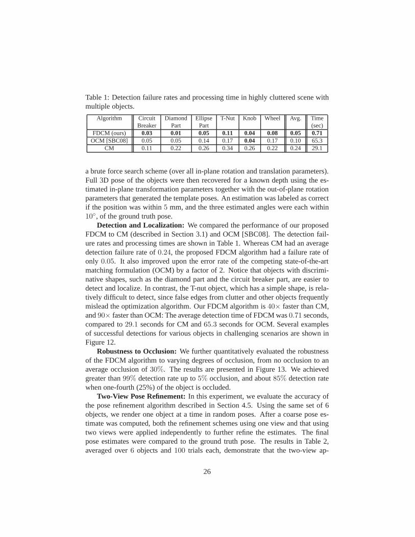
Table 1: Detection failure rates and processing time in highly cluttered scene withmultiple objects.

Algorithm Circuit Diamond Ellipse T-Nut Knob Wheel Avg. TimeBreaker Part Part (sec)

FDCM (ours) 0.03 0.01 0.05 0.11 0.04 0.08 0.05 0.71OCM [SBC08] 0.05 0.05 0.14 0.17 0.04 0.17 0.10 65.3

CM 0.11 0.22 0.26 0.34 0.26 0.22 0.24 29.1

a brute force search scheme (over all in-plane rotation and translation parameters).Full 3D pose of the objects were then recovered for a known depth using the es-timated in-plane transformation parameters together withthe out-of-plane rotationparameters that generated the template poses. An estimation was labeled as correctif the position was within5 mm, and the three estimated angles were each within10◦, of the ground truth pose.

Detection and Localization: We compared the performance of our proposedFDCM to CM (described in Section 3.1) and OCM [SBC08]. The detection fail-ure rates and processing times are shown in Table 1. Whereas CM had an averagedetection failure rate of0.24, the proposed FDCM algorithm had a failure rate ofonly 0.05. It also improved upon the error rate of the competing state-of-the-artmatching formulation (OCM) by a factor of 2. Notice that objects with discrimi-native shapes, such as the diamond part and the circuit breaker part, are easier todetect and localize. In contrast, the T-nut object, which has a simple shape, is rela-tively difficult to detect, since false edges from clutter and other objects frequentlymislead the optimization algorithm. Our FDCM algorithm is40× faster than CM,and90× faster than OCM: The average detection time of FDCM was0.71 seconds,compared to29.1 seconds for CM and65.3 seconds for OCM. Several examplesof successful detections for various objects in challenging scenarios are shown inFigure 12.

Robustness to Occlusion:We further quantitatively evaluated the robustnessof the FDCM algorithm to varying degrees of occlusion, from no occlusion to anaverage occlusion of30%. The results are presented in Figure 13. We achievedgreater than99% detection rate up to5% occlusion, and about85% detection ratewhen one-fourth (25%) of the object is occluded.

Two-View Pose Refinement:In this experiment, we evaluate the accuracy ofthe pose refinement algorithm described in Section 4.5. Using the same set of 6objects, we render one object at a time in random poses. Aftera coarse pose es-timate was computed, both the refinement schemes using one view and that usingtwo views were applied independently to further refine the estimates. The finalpose estimates were compared to the ground truth pose. The results in Table 2,averaged over6 objects and100 trials each, demonstrate that the two-view ap-

26

(b) (c) (d)(a)

Diamond Part

Circuit Breaker Part

T-Nut

Ellipse Part

Knob

Wheel

Figure 12: Examples of successful pose estimation on the synthetic dataset.(a) Photo of each part. (b) Sample depth-edge template. (c) Rendered query image.(d) Pose estimation result.

27

0 5 10 15 20 25 300.6

0.7

0.8

0.9

1

Degree of Occlusion

Det

ectio

n R

ate

Figure 13: Detection rate versus percentage of occlusion.

Table 2: Comparison of the average absolute pose estimationerror between theone-view and two-view approaches.

Average tX tY tZ θX θY θZabsolute error mm mm mm degree degree degree

1 View 0.127 0.165 1.156 0.674 0.999 0.3492 View 0.094 0.096 0.400 0.601 0.529 0.238

proach outperformed the one-view approach. In the renderedimages,1 mm cor-responded to about6.56 pixels on the image plane, indicating that the two-viewestimate achieves sub-pixel accuracy.

5.1.2 Real Examples

Object Detection and Pose Estimation in Cluttered Scenes:To quantitativelyevaluate performance, we performed several real experiments. Six different typesof objects were laid one on top of another in a cluttered manner as shown in Fig-ure 14. We then extracted depth edges using the MFC and performed object detec-tion and pose estimation on the resulting depth-edge images. In each trial of thisexperiment, we used the system to detect a single instance ofan object type. Overseveral hundred trials, the average detection rate was95%. Shown in Figure 14are some typical example trials of this experiment. On each image, we overlay thesilhouettes of the detector outputs for three different object types. Notice that someof the parts have no texture, while others are quite specular. In such challengingscenarios, methods based on traditional image edges (e.g.,Canny edges) usuallyfail, but the MFC enables us to robustly extract depth edges.Also notice that sincethe depth edge features are not affected by texture, our method works robustly evenfor parts that have artificial texture painted on them. This indicates that the methodcan work in the presence of oil, grime, or dirt (which are all common in industrial

28

Figure 14: Results using real examples. The system detectedand accurately esti-mated the pose for specular (shiny metal) objects, textureless objects (such as theones in the bottom center image), and objects that have potentially misleading tex-ture painted on them (such as the ones in the bottom right image). Overlaid on eachimage is the top detector output for each of three different object types.

environments), all of which add artificial texture to the surface of objects.Statistical Evaluation: In order to statistically evaluate the accuracy of the

proposed system, we need a method of independently obtaining the 3D groundtruth pose of the object. Since there was no simple way of obtaining this (es-pecially when objects were stacked on top of each other or piled in a bin), weinstead devised a method to evaluate the consistency of poseestimate across multi-ple viewpoints of the camera. We placed an object in the sceneand commanded therobot arm to move to several rotations and translations, so that data are collectedwhen the camera is pointing at the object using many different camera poses. Thecamera poses were maintained such that the distance along the z-axis between thecamera and the object is±10 mm from the hypothesized distancetz that was usedto generate the database (Section 4.3). From each camera pose, MFC images werecaptured, and our algorithm was used to estimate the pose of the object in the cam-era coordinate system. Since the object is static, the estimated pose of the objectin the world coordinate system should be identical irrespective of the viewpointof the MFC. For each view, the estimated pose of the object wastransformed tothe world coordinate system using the known position and orientation of the robotarm. We repeated this experiment for7 different objects, with25 trials for each ob-ject (the object was placed in a different pose for each trial). During each of theseindependent trials, the robot arm was moved to40 different viewpoints in order

29

Figure 15: Results from real examples. Histograms of deviations from the medianpose estimate, in mm (top) and degrees (bottom), across multiple trials of poseestimation.

to evaluate the consistency of the pose estimates. The histogram of the deviationsfrom the median pose estimate is shown in Figure 15. The results demonstrate thatthe algorithm computes consistent estimates, with a standard deviation of less than0.5 mm in the in-plane directions(x, y) and about2 degrees in each of the threeorientation angles. The standard deviation of the estimatein thez direction (alongthe optical axis of camera) is slightly larger (approximately 1.2 mm).

Effect of Depth Variation: In our experiments, the system was optimizedfor a part container with a depth variation of40 mm and a distance along thez-axis of275 mm from the camera to the top of the part container. As explained inSection 4.3, the pose estimation algorithm requires a roughvalue of the distance,tz, from the camera to the objects along thez-axis. In this experiment, we analyzehow deviations of the true object distance from the hypothesized distancetz affectpose estimation accuracy.

We placed a single object in the scene and performed pose estimation at severaldifferent camera poses with offsets along thez-axis from the hypothesized distanceof 275 mm. At eachz offset (height), we repeated the pose estimation for100trials by randomly changing the camera pose in the(x, y) directions. As in theprevious experiment, we used the median pose estimate as theground truth pose.An estimate is labeled as correct if the translation error, computed as the Euclideandistance between the(x, y, z) translation vectors, is less than3 mm and the rotationerror, computed as the geodesic distance between two 3D rotations, is less than8◦.

30

−40 −30 −20 −10 0 10 20 30 40 50

80

85

90

95

100

Camera Height Offset [mm]

Suc

cess

Rat

e [%

]

Figure 16: Effect of depth variation on pose estimation.

The accuracy of the system is shown in Figure 16. The pose estimation algorithmis quite robust to depth variations between[−20,+50] mm, which is significantlylarger than our target capture range. Outside of this range,our two-view poserefinement algorithm failed to converge to the true solutionfor several trials, due tothe incorrect distance assumption causing large projection errors. This experimentsuggests that for part containers with larger depth variations, coarse pose estimationshould be performed at multiple scales, targeting different depths, to get a betterinitial depth estimation. Alternatively, we could move therobot arm and changethe height of the capture position based on previous object pose estimates in orderto maintain a roughly constant distance between the camera and the objects.

5.1.3 Bin-Picking System Performance

We evaluated the performance of bin picking using the robotic system shown inFigure 5. Extension 1 demonstrates our system accomplishing this task in real time.Figure 5 shows a part container (bin) containing a large number of circuit breakerparts. The gripper (end effector) of the robot arm is designed to grasp each of theobjects by first inserting its three metal pins in the closed state through a hole in theobject. The gripper then opens by moving the three pins radially outward, therebyexerting outward horizontal forces on the inside edges of the hole. The gripper hasa diameter of3 mm in its closed state, while the hole in the object has a diameter ofabout6 mm. Therefore, in order to successfully insert the gripper inside the hole(before lifting the object), the pose estimate error in the(x, y) directions must beless than1.5 mm. If the pose estimate error is greater, the pins will not beinsertedinto the hole, resulting in a failure to grasp the object.

31

Our system was able to successfully guide the robot arm in thegrasping task,achieving a grasping success rate of94% over several hundred trials. There weretwo main causes for the grasping failures in6% of the trials: (1) This particulartarget object has very similar depth edges when it is flipped upside-down, whichoccasionally led to inaccurate pose estimates; (2) Even when the pose estimationwas correct, the hole of the object was occasionally occluded by other objects,resulting in a grasping failure. It is important to note thatall of these graspingfailures were detected by the error-detection process using the gripper camera, sothey did not affect the subsequent assembly task. Among the instances of success-ful grasping, a few trials resulted in the object being picked up by the gripper inan incorrect pose, due to interference from neighboring objects during the pickupprocess. These cases were also detected and were corrected automatically by oursystem using the gripper camera and our process for pose estimation and correctionin the gripper (described in Section 4.6).

Processing Time:The entire pose estimation process requires less than1 sec-ond for an object in an extremely cluttered environment (on an Intel quad-core3.4Ghz CPU with3 GB memory). The decomposition of processing time is0.6 sec-onds for FDCM and0.3 seconds for the multi-view pose refinement algorithm. Asshown in Extension 1, almost all of the computation occurs during robot motion,so the computation time has almost no effect on the system operation speed. Inenvironments with minimal clutter, the algorithm runs about twice as fast, sincethere are significantly fewer edges in the captured images.

5.1.4 Pose Estimation in the Gripper

To evaluate the system’s potential for error correction in the gripper, we measurethe accuracy of pose estimation in the gripper using different numbers of views. Inthis experiment, we picked up circuit breaker parts from thepart container as de-scribed in Section 5.1.3. After each pickup, we captured8 images at different wristrotation angles, as shown in Figure 17, using the gripper camera and foregroundextraction during robot motion (described in Section 4.6).We performed the poserefinement algorithm (Section 4.5) using from 1–8 views (forthese experiments,we used the ideal pose of the object as the initial guess).

Figure 18 shows pose estimation errors using different numbers of views. Sincethe ground truth of the object pose in the gripper is not available, we used the posethat was estimated using all8 views as the ground truth, and compared it withthe poses estimated using different numbers (1–7) of views. The plots show theaverage estimation errors and standard deviations of theseestimation errors (errorbars) over100 trials. Similar to our observations from synthetic data (shown inTable 2), the translation errors on real data are smaller fortwo-view estimationthan for one-view estimation (see Figure 18, left). Two-view pose estimation is

32

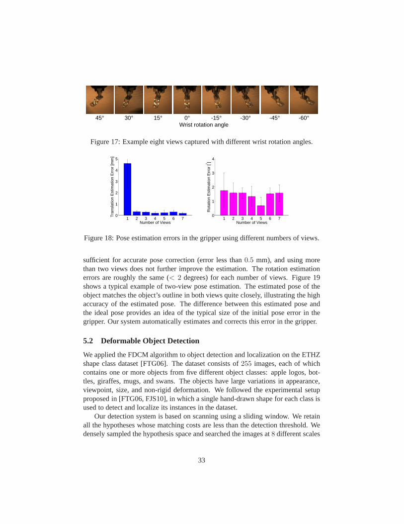
Wrist rotation angle45° 30° 15° 0° -15° -30° -45° -60°

Figure 17: Example eight views captured with different wrist rotation angles.

1 2 3 4 5 6 70

1

2

3

4

5

Tra

nsla

tion

Est

imat

ion

Err

or [m

m]

Number of Views1 2 3 4 5 6 7

0

1

2

3

4

Rot

atio

n E

stim

atio

n E

rror

[° ]

Number of Views

Figure 18: Pose estimation errors in the gripper using different numbers of views.

sufficient for accurate pose correction (error less than0.5 mm), and using morethan two views does not further improve the estimation. The rotation estimationerrors are roughly the same (< 2 degrees) for each number of views. Figure 19shows a typical example of two-view pose estimation. The estimated pose of theobject matches the object’s outline in both views quite closely, illustrating the highaccuracy of the estimated pose. The difference between thisestimated pose andthe ideal pose provides an idea of the typical size of the initial pose error in thegripper. Our system automatically estimates and corrects this error in the gripper.

5.2 Deformable Object Detection

We applied the FDCM algorithm to object detection and localization on the ETHZshape class dataset [FTG06]. The dataset consists of255 images, each of whichcontains one or more objects from five different object classes: apple logos, bot-tles, giraffes, mugs, and swans. The objects have large variations in appearance,viewpoint, size, and non-rigid deformation. We followed the experimental setupproposed in [FTG06, FJS10], in which a single hand-drawn shape for each class isused to detect and localize its instances in the dataset.

Our detection system is based on scanning using a sliding window. We retainall the hypotheses whose matching costs are less than the detection threshold. Wedensely sampled the hypothesis space and searched the images at8 different scales

33

1st View 2nd View

Ideal PoseEstimated Pose

Figure 19: Two-view pose estimation in the gripper. The ideal pose is used as theinitial guess and refined to give the estimated pose. (Both poses are superimposedon the input images of the two views).

and3 different aspect ratios. The ratio between two consecutivescales is1.2 andbetween consecutive aspect ratios is1.1. We performed non-maximal suppressionby retaining only the lowest-cost hypothesis among any group of detections thathave significant spatial overlap.

In Figure 20, we plot detection rate vs. false positives per image. The curveis generated via altering the detection threshold for the matching cost. We com-pared our approach with OCM [SBC08] and two recent studies byFerrari et.al. [FTG06, FJS10]. Our approach outperforms OCM at all the false positive ratesand is comparable to [FJS10]. Compared to [FJS10], our results are better fortwo classes (giraffes and bottles) and slightly worse for the swans class, while fortwo other classes (apple logos and mugs), the numbers are almost identical. Asshown in the detection examples (Figure 21), object localization is highly accu-rate. Note that [ZWWS08] and [RJM08] report slightly betterperformance on thisdataset, but we could not include their results in our graphsbecause their resultswere only reported in graphical format (as precision-recall curves). Also note thatthese methods are orders of magnitude slower than FDCM.

Complexity Comparison: The average number of points in the shape tem-plates were1, 610, computed over five classes. Our line-based representationusedan average of39 line segments per class. Note that the number of lines per classprovides an upper bound on the number of computations required. Since the algo-rithm retrieves only the hypotheses having a smaller cost than the detection thresh-old, the summation was terminated for a hypothesis if the cost exceeded this value.By using this bound in the hypothesis domain (see Section 3.6.1 for more details),on average only14 line segments were evaluated per hypothesis.

The average evaluation time for a single hypothesis was0.40 µs using FDCM,whereas this process took51.50 µs for OCM and17.59 µs for CM. The proposed

34

Figure 20: Receiver operating characteristic (ROC) curveson the ETHZ shapedataset comparing our proposed approach to OCM [SBC08] and two recent studiesby Ferrari et. al. [FTG06, FJS10].

35

Figure 21: Several localization results on the ETHZ shape dataset. The images aresearched using a single hand-drawn shape shown in the lower right of the imagesin the rightmost column.

method is43× faster than chamfer matching and127× faster than oriented chamfermatching. Note that the speed up is more significant for larger-sized templates,since our cost computation is insensitive to the template size, whereas the cost ofstandard chamfer matching increases linearly.

On average, we evaluated1.05 million hypotheses per image, which took0.42seconds. Using the bound in the spatial domain presented in Section 3.6.2 enabled91% of the hypotheses to be skipped, reducing the average evaluation time perimage to0.39 seconds. Note that the speedup is not proportional to the fractionof hypotheses skipped because in order to use the bound in thespatial domain, wecould no longer use the bound in the hypothesis domain (Section 3.6.1).

36

Table 3: Pose estimation errors on three action sequences. Errors are measured asthe mean absolute pixel distance from the ground truth marker locations.

Algorithm Walking Jogging Boxing AverageFDCM (ours) 7.3 12.5 9.7 9.8

OCM [SBC08] 15.0 15.3 13.6 14.6CM 9.3 13.6 10.6 11.2

Figure 22: Human pose estimation results.First row: Walking sequence.Secondrow: Jogging and boxing sequences. Estimated poses and contoursare overlayedon the images.

5.3 Human Pose Estimation

We utilized our shape-matching framework for human pose estimation, which is ahighly challenging task due to the large set of possible articulations of the humanbody. As proposed in [MM02], we matched a gallery of human shapes that haveknown poses to each test image. Due to articulation, the sizeof the pose galleryneeded for accurate pose estimation is large. Hence, it becomes increasingly im-portant to have an efficient matching algorithm that can copewith backgroundclutter.

The experiments were performed on the HumanEva dataset [SB06a], whichcontains video sequences of multiple human subjects performing various activitiescaptured from different viewing directions. The ground truth locations of humanjoints at each image were extracted using attached markers.Shape gallery tem-plates were acquired in two steps. First, we computed the human silhouettes via

37

HumanEva background subtraction code. Then, using the Canny edges aroundthe extracted silhouette outlines, we obtained the shape templates. We performedthe experiment on video sequences from one subject of three actions: walking,jogging, and boxing. For each action, we included all of the images from thesubject’s training sequence (about1, 000–2, 000 images) in the shape gallery. Weused this to estimate the subject’s pose in the corresponding validation sequence.As we extracted Canny edges directly from the validation images, they includedus significant amount of background clutter. The best shape template, togetherwith its scale and location, were then retrieved via the matching framework. Wequantitatively evaluated the mean absolute error between the ground truth markerlocations and the estimated pose on the image plane. The results, presented in Ta-ble 3, demonstrate significant improvements in accuracy compared to OCM andCM. Our proposed approach can evaluate more than1.1 million hypotheses persecond, whereas CM and OCM can evaluate only31, 000 and14, 000 hypothesesper second, respectively. Examples of pose estimation are shown in Figure 22.

The code for FDCM can be downloaded from the first author’s website.

6 Conclusion

We presented a practical robotic system that uses novel computer vision hardwareand algorithms for detection and 3D pose estimation of industrial parts in a clut-tered bin. Our implementation of the system on a robotic arm achieves accuracieson the order of 1 mm (reduced to less than 0.5 mm with automaticerror correction)and2◦, with a total processing time of less than 1 second. Given a CAD model,a new object can be integrated into our system in less than 10 minutes. Our goalwith this line of research is to make substantial progress towards more versatileand easy-to-customize robotic bin-picking systems.

Acknowledgements

We thank Amit Agrawal, Srikumar Ramalingam, Ramesh Raskar,Keisuke Kojima,and Jay Thornton for their helpful comments and suggestions. Special thanks toJohn Barnwell for his invaluable help with the hardware. This research was mostlyconducted at MERL with support from MERL. Ming-Yu Liu and Ashok Veer-araghavan contributed to the work while they were at MERL. AtRice University,Ashok Veeraraghavan was partially supported by NSF grant NSF 1117939. RamaChellappa was supported by MURI from the Office of Naval Research under theGrant N00014-08-I-0638.

38

A Index to Multimedia Extensions

The multimedia extensions to this article are at: http://www.ijrr.org.

Table 4: Multimedia ExtensionsExtension Type Description

1 Video

System demo video. In the video, we demonstratethe robustness and real-time performance of theproposed system for picking up parts in a chal-lenging setting. Through showing 10 consecutivepickups of an industrial part from a highly clut-tered bin, we illustrate the applicability of the pro-posed system to industrial assembly. Each of themajor components of the algorithm is highlighted.The video also contains several close-up views ofthe pickups.

References

[ASBR10] Amit Agrawal, Yu Sun, John Barnwell, and Ramesh Raskar. Vision-guided robot system for picking objects by casting shadows.Interna-tional Journal of Robotics Research, 29:155–173, February 2010.

[AT06] Ankur Agarwal and Bill Triggs. Recovering 3d human pose frommonocular images.IEEE Transactions on Pattern Analysis and Ma-chine Intelligence, 28(1):44–58, 2006.

[BB09] Csaba Beleznai and Horst Bischof. Fast human detection in crowdedscenes by contour integration and local shape estimation. In Proceed-ings of the IEEE Conference on Computer Vision and Pattern Recog-nition, pages 2246–2253, 2009.

[BBM05] Alexander C. Berg, Tamara L. Berg, and Jitendra Malik. Shape match-ing and object recognition using low distortion correspondences. InProceedings of the IEEE Conference on Computer Vision and PatternRecognition, pages 26–33, 2005.

[BETG08] Herbert Bay, Andreas Ess, Tinne Tuytelaars, and Luc J. Van Gool.Speeded-up robust features (surf).Computer Vision and Image Un-derstanding, 110(3):346–359, 2008.

39

[BJ03] Ronen Basri and David W. Jacobs. Lambertian reflectance and lin-ear subspaces.IEEE Transactions on Pattern Analysis and MachineIntelligence, 25(2):218–233, 2003.

[BMP02] Serge Belongie, Jitendra Malik, and Jan Puzicha. Shape matchingand object recognition using shape contexts.IEEE Transactions onPattern Analysis and Machine Intelligence, 24(4):509–522, 2002.

[BN10] Prabin Bariya and Ko Nishino. Scale-hierarchical 3dobject recogni-tion in cluttered scenes. InProceedings of the IEEE Conference onComputer Vision and Pattern Recognition, 2010.

[BTBW77] Harry G Barrow, Jay Martin Tenenbaum, Robert Coy Bolles, and He-len C Wolf. Parametric correspondence and chamfer matching: Twonew techniques for image matching. InProceedings of the 5th in-ternational joint conference on Artificial intelligence, pages 659–663,1977.

[BV04] Stephen Boyd and Lieven Vandenberghe.Convex Optimization. Cam-bridge University Press, March 2004.

[Can86] John Canny. A computational approach to edge detection. IEEETransactions on Pattern Analysis and Machine Intelligence, 8(6):679–698, 1986.

[CSD+10] Yan Cui, Sebastian Schuon, Chan Derek, Sebastian Thrun,and Chris-tian Theobalt. 3d shape scanning with a time-of-flight camera. InProceedings of the IEEE Conference on Computer Vision and PatternRecognition, 2010.

[DBdFF02] Pinar Duygulu, Kobus Barnard, Joao F. G. de Freitas, and David A.Forsyth. Object recognition as machine translation: Learning a lex-icon for a fixed image vocabulary. InProceedings of the EuropeanConference on Computer Vision, pages 97–112, 2002.

[DCS09] Oscar Danielsson, Stefan Carlsson, and Josephine Sullivan. Auto-matic learning and extraction of multi-local features. InProceedingsof the IEEE International Conference on Computer Vision, 2009.

[DD92] Daniel DeMenthon and Larry Davis. Model-based object pose in 25lines of code. InProceedings of the European Conference on Com-puter Vision, pages 335–343, 1992.

40

[DT05] Navneet Dalal and Bill Triggs. Histograms of oriented gradients forhuman detection. InProceedings of the IEEE Conference on Com-puter Vision and Pattern Recognition, pages 886–893, 2005.

[DUNI10] Bertram Drost, Markus Ulrich, Nassir Navab, and Slobodan Ilic.Model globally, match locally: Efficient and robust 3d object recog-nition. In Proceedings of the IEEE Conference on Computer Visionand Pattern Recognition, pages 998–1005, 2010.

[FB81] Martin A. Fischler and Robert C. Bolles. Random sample consensus:a paradigm for model fitting with applications to image analysis andautomated cartography.Graphics and Image Processing, 24(6):381–395, 1981.

[FFFP06] Li Fei-Fei, R. Fergus, and P. Perona. One-shot learning of objectcategories.IEEE Transactions on Pattern Analysis and Machine In-telligence, 28(4):594–611, 2006.

[FFJS08] V. Ferrari, L. Fevrier, F. Jurie, and C. Schmid. Groups of adjacentcontour segments for object detection.IEEE Transactions on PatternAnalysis and Machine Intelligence, 30(1):36–51, 2008.

[FH04] Pedro Felzenszwalb and Daniel Huttenlocher. Distance transforms ofsampled functions. Technical Report TR2004-1963, CornellComput-ing and Information Science, 2004.

[FJS10] Vittorio Ferrari, Frederic Jurie, and Cordelia Schmid. From images toshape models for object detection.International Journal of ComputerVision, 87:284–303, 2010.

[FS07] Pedro Felzenszwalb and Joshua Schwartz. Hierarchical matching ofdeformable shapes. InProceedings of the IEEE Conference on Com-puter Vision and Pattern Recognition, 2007.

[FTG06] Vittorio Ferrari, Tinne Tuytelaars, and Luc Van Gool. Object detec-tion by contour segment networks. InProceedings of the EuropeanConference on Computer Vision, volume 3953, pages 14–28, 2006.

[Gav98] Dariu M. Gavrila. Multi-feature hierarchical template matching usingdistance transforms. InProceedings of the IEEE International Con-ference on Pattern Recognition, pages 439–444, 1998.

[GLP84] Eric Grimson and Tomas Lozano-Perez. Model-based recognition andlocalization from sparse range or tactile data.International Journalof Robotics Research, 3:3–35, 1984.

41

[Hor87] Berthold K. P. Horn. Closed-form solution of absolute orientationusing unit quaternions.Journal of the Optical Society A, 4(4):629–642, 1987.

[JH99] Andrew E. Johnson and Martial Hebert. Using spin images for effi-cient object recognition in cluttered 3d scenes.IEEE Transactions onPattern Analysis and Machine Intelligence, 21(5):433–449, 1999.

[LJ07] Haibin Ling and David W. Jacobs. Shape classificationusing theinner-distance.IEEE Transactions on Pattern Analysis and MachineIntelligence, 29(2):286–299, 2007.

[Low87] David Lowe. Three-dimensional object recognitionfrom single two-dimensional images.Artificial Intelligence, 31(3):355–395, 1987.

[Low91] David Lowe. Fitting parameterized three-dimensional models to im-ages. IEEE Transactions on Pattern Analysis and Machine Intelli-gence, 13(5):441–450, 1991.

[Low04] David G. Lowe. Distinctive image features from scale-invariant key-points. International Journal of Computer Vision, 60(2):91–110,2004.

[LSP06] Svetlana Lazebnik, Cordelia Schmid, and Jean Ponce. Beyond bags offeatures: Spatial pyramid matching for recognizing natural scene cat-egories. InProceedings of the IEEE Conference on Computer Visionand Pattern Recognition, pages 2169–2178, 2006.

[LTV +10] Ming-Yu Liu, Oncel Tuzel, Ashok Veeraraghavan, Rama Chellappa,Amit Agrawal, and Haruhisa Okuda. Pose estimation in heavy clutterusing a multi-flash camera. InProceedings of the IEEE InternationalConference on Robotics and Automation, 2010.

[LTVC10] Ming-Yu Liu, Oncel Tuzel, Ashok Veeraraghavan, and Rama Chel-lappa. Fast directional chamfer matching. InProceedings of the IEEEConference on Computer Vision and Pattern Recognition. IEEE Com-puter Society, 2010.

[MM02] Greg Mori and Jitendra Malik. Estimating human body configura-tions using shape context matching. InProceedings of the EuropeanConference on Computer Vision, volume 3, 2002.

[MREM04] Greg Mori, Xiaofeng Ren, Alexei A. Efros, and Jitendra Malik. Re-covering human body configurations: Combining segmentation and

42

recognition. InProceedings of the IEEE Conference on ComputerVision and Pattern Recognition, pages 326–333, 2004.

[NFF07] Juan Carlos Niebles and Li Fei-Fei. A hierarchical model of shapeand appearance for human action classification. InProceedings of theIEEE Conference on Computer Vision and Pattern Recognition, 2007.

[NPK96] Bradley Nelson, N.P. Papanikolopoulos, and Pradeep Khosla. Roboticvisual servoing and robotic assembly tasks.IEEE Robotics and Au-tomation Magazine, 3(1):23–31, June 1996.

[OH97] Clark F. Olson and Daniel P. Huttenlocher. Automatictarget recogni-tion by matching oriented edge pixels.IEEE Transactions on PatternAnalysis and Machine Intelligence, 6(1):103–113, 1997.

[OT01] Aude Oliva and Antonio Torralba. Modeling the shape of the scene: Aholistic representation of the spatial envelope.International Journalof Computer Vision, 42(3):145–175, 2001.

[RJM08] Saiprasad Ravishankar, Arpit Jain, and Anurag Mittal. Multi-stagecontour based detection of deformable objects. InProceedings of theEuropean Conference on Computer Vision, pages 483–496, 2008.

[RTF+04] Ramesh Raskar, Kar-Han Tan, Rogerio Feris, Jingyi Yu, and MatthewTurk. Non-photorealistic camera: depth edge detection andstylizedrendering using multi-flash imaging.ACM Transactions on Graphics,23(3):679–688, 2004.

[SB06a] Leonid Sigal and Michael J. Black. Humaneva: Synchronized videoand motion capture dataset for evaluation of articulated human mo-tion. Technical report, Brown University, 2006.

[SB06b] Leonid Sigal and Michael J. Black. Measure locally,reason globally:Occlusion-sensitive articulated pose estimation. InProceedings of theIEEE Conference on Computer Vision and Pattern Recognition, pages2041–2048, 2006.

[SBC08] Jamie Shotton, Andrew Blake, and Roberto Cipolla. Multi-scale cat-egorical object recognition using contour fragments.IEEE Trans-actions on Pattern Analysis and Machine Intelligence, 30(7):1270–1281, 2008.

[SI73] Y. Shirai and H. Inoue. Guiding a robot by visual feedback in assem-bling tasks.Pattern Recognition, 5(2):99 –108, 1973.

43

[SM92] Fridtjof Stein and Gerard Medioni. Structural indexing: Efficient 3-dobject recognition.IEEE Transactions on Pattern Analysis and Ma-chine Intelligence, 14(2):125 –145, 1992.

[SS03] Daniel Scharstein and Richard Szeliski. High-accuracy stereo depthmaps using structured light. InProceedings of the IEEE Conferenceon Computer Vision and Pattern Recognition, 2003.

[STFW05] Erik B. Sudderth, Antonio Torralba, William T. Freeman, and Alan S.Willsky. Learning hierarchical models of scenes, objects,and parts.In Proceedings of the IEEE International Conference on ComputerVision, pages 1331–1338, 2005.

[TPM08] Oncel Tuzel, Fatih Porikli, and Peter Meer. Pedestrian detection viaclassification on riemannian manifolds.IEEE Transactions on PatternAnalysis and Machine Intelligence, 30(10):1713–1727, 2008.

[TSTC03] Arasanathan Thayananthan, Bjorn Stenger, PhilipH. S. Torr, andRoberto Cipolla. Shape context and chamfer matching in clutteredscenes. InProceedings of the IEEE Conference on Computer Visionand Pattern Recognition, pages 127–133, 2003.

[Vis] VisionPro. http://www.cognex.com/visionpro/.Cognex.

[VJ01] Paul Viola and Michael Jones. Rapid object detectionusing a boostedcascade of simple features. InProceedings of the IEEE Conference onComputer Vision and Pattern Recognition, volume 1, pages 511–518,2001.

[Zha94] Zhengyou Zhang. Iterative point matching for registration of free-form curves and surfaces.International Journal of Computer Vision,13(2):119–152, 1994.

[ZWWS08] Qihui Zhu, Liming Wang, Yang Wu, and Jianbo Shi. Contour con-text selection for object detection: A set-to-set contour matching ap-proach. InProceedings of the European Conference on ComputerVision, pages 774–787, 2008.

44