Fast Ninomiya-Victoir calibration of ... - … cation Calibration Ninomiya-Victoir DMR simulation...

Specification Calibration Ninomiya-Victoir DMR simulation Daily fitting

Fast Ninomiya-Victoir calibration of theDouble-Mean-Reverting Model

Jim Gatheral(joint work with Christian Bayer and Morten Karlsmark)

Stochastic Processes and their Statistics in FinanceOkinawa, Japan

October 31, 2013


Overview of this talk

Specification of the DMR model

Calibration of model parameters

The Ninomiya-Victoir scheme and extensions

Simulation of the DMR model

Examples of model fits to options data

Summary and conclusions


Modeling SPX and VIX

It is well-known that the empirically observed implied volatilitysurface is not consistent with Black-Scholes.

Many models have been proposed proposed to fit marketimplied volatilities better and describe the dynamics of thevolatility surface.

For example, local volatility models, Levy models, stochasticvolatility models, stochastic volatility models with jumps andso on.

With the advent of trading in VIX options in 2006 however,marginal risk-neutral densities of forward volatilities of SPXbecame effectively observable, substantially constrainingpossible choices of volatility dynamics.

Various authors have since proposed models that price bothoptions on SPX and options on VIX more or less consistentlywith the market.


The DMR model

In [my Bachelier 2008 presentation], a specific three factorvariance curve model was introduced with dynamics motivatedby economic intuition for the empirical dynamics of thevariance.

In this double-mean-reverting or DMR model, the dynamicsare given by

dSt =√

vtStdW 1t , (1a)

dvt = κ1 (v ′t − vt) dt + ξ1 vα1t dW 2

t , (1b)

dv ′t = κ2 (θ − v ′t) dt + ξ2 v ′tα2 dW 3

t , (1c)

where the Brownian motions Wi are all in general correlatedwith E[dW i

t dW jt ] = ρij dt.


Qualitative features of the DMR model

Instantaneous variance v mean-reverts to a level v ′ that itselfmoves slowly over time with the state of the economy,mean-reverting to the long-term mean level θ.

Also, it is a stylized fact that the distribution of volatility(whether realized or implied) should be roughly lognormal

When the model is calibrated to market option prices, we findthat indeed α1 ≈ 1 consistent with this stylized fact.

As we will see later, the DMR model calibrated jointly to SPXand VIX options markets fits pretty well.


Computations in the DMR model

One drawback of the DMR model is that calibration is noteasy

No closed-form solution for European options exists so finitedifference or Monte Carlo methods need to be used to priceoptions.Calibration is therefore slow.

In [my Bachelier 2008 presentation], the DMR model iscalibrated using an Euler-Maruyama Monte Carlo scheme withthe partial truncation step of [Lord, Koekkoek, and van Dijk].

In this talk, we show how to apply the Monte Carlo scheme of[Ninomiya and Victoir] to the calibration of the DMR model,substantially improving calibration time.


Model calibration

The DMR model has many parameters:

One could argue that it is both mis-specified andover-parameterized.

In [my Bachelier 2008 presentation], the parameters of theDMR model were calibrated to the VIX and SPX optionsmarkets with a sequence of steps that we will now individuallydescribe.


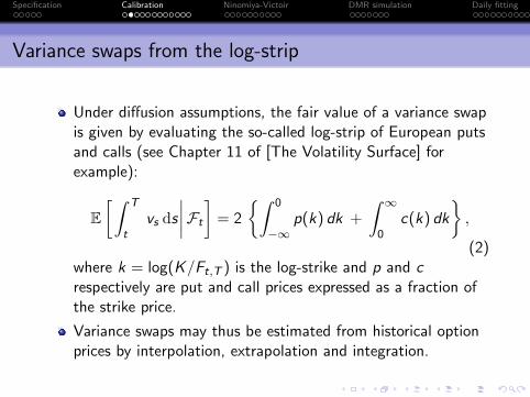
Variance swaps from the log-strip

Under diffusion assumptions, the fair value of a variance swapis given by evaluating the so-called log-strip of European putsand calls (see Chapter 11 of [The Volatility Surface] forexample):

E[∫ T

tvs ds

∣∣∣∣Ft

]= 2

{∫ 0

−∞p(k) dk +

∫ ∞0

c(k) dk

},

(2)where k = log(K/Ft,T ) is the log-strike and p and crespectively are put and call prices expressed as a fraction ofthe strike price.

Variance swaps may thus be estimated from historical optionprices by interpolation, extrapolation and integration.


Estimation of κ1, κ2, θ and ρ23

In the DMR model, the fair strike of a variance swap is givenby the expression

E[∫ T

tvs ds

∣∣∣∣Ft

]= θ τ + (vt − θ)

1− e−κ1 τ

κ1

+ (v ′t − θ)κ1

κ1 − κ2

{1− e−κ2 τ

κ2− 1− e−κ1 τ

κ1

}(3)

which is affine in the state variables vt and v ′t .

Fixing θ, κ1 and κ2, and given daily variance swap estimates,time series of vt and v ′t may be imputed by linear regression.

Optimal values of θ, κ1 and κ2 are obtained by minimizingmean squared differences between the fitted and actualvariance swap curves.


Calibrated parameters

With daily data from January 2001 to April 2008, the optimalchoice of parameters was found to be

θ = 0.078,

κ1 = 5.5,

κ2 = 0.10.

The correlation ρ23 between W 2t and W 3

t was then estimatedas the historical correlation between the series vt and v ′t . Theestimated value was

ρ23 = 0.59.


Motivation for fitting SABR

It seems that volatility dynamics are roughly lognormalOption prices and time series analysis lead us to the sameconclusion.

The SABR model of[Hagan, Kumar, Lesniewski, and Woodward] is the simplestpossible lognormal stochastic volatility model

And there is an accurate closed-form approximation to impliedvolatility.

The lognormal SABR process is:

dS

S= Σ dZ

dΣ

Σ= ν dW (4)

with 〈dZ , dW 〉 = ρ dT .Fitting SABR might allow us to impute effective parametersfor a more complicated model.


The SABR formula

As shown originally by Hagan et al., to lowest order in time toexpiration, the solution to (4) in terms of the Black-Scholesimplied volatility σBS is approximated by:

σBS (k) = σ0 f

(k

σ0

)where k := log(K/F ) is the log-strike and

f (y) = − ν y

log

(√ν2 y2+2 ρ ν y+1−ν y−ρ

1−ρ

)It turns out that this simple formula is reasonably accurate forlonger expirations too.

Note that the formula is independent of time to expiration T .


The term structure of ν

As of 25-Apr-2008, plot fitted ν for each slice against Texp:

0.0 0.5 1.0 1.5 2.0 2.5

0.0

0.5

1.0

1.5

2.0

Expiry (years)

Effe

ctiv

e SA

BR v

ol o

f vol

(i)

0.0 0.5 1.0 1.5 2.0 2.5

0.0

0.5

1.0

1.5

2.0

The red line is the function 0.501√T

.


Estimation of the exponents α1 and α2

The exponents α1 and α2 control how volatility of volatilitychanges with the volatility level.

To obtain a proxy for the volatility of volatility we note thatthe lognormal SABR model (with β = 1) tends to fit the smileat any given expiration very well.

One of the SABR parameters is the volatility of volatility ν.

We note further that empirically, the term structure of ν isgiven by

ν(τ) ≈ νeff√τ

νeff may then be used as a proxy for volatility of volatility.

We use VIX as a proxy for the level of volatility.


SABR fits to SPX: νeff

Figure 1: Computing νeff every day for seven years gives the followingtime-series plot:

0.0

0.2

0.4

0.6

0.8

Effe

ctiv

e SA

BR v

ol o

f vol

2002 2004 2006 2008


Observations from νeff time-series

Lognormal volatility of volatility νeff is empirically ratherstable

The dynamics of the volatility surface imply that volatility isroughly lognormal.

Can we see any patterns in the plot?

For example, does νeff depend on the level of volatility?


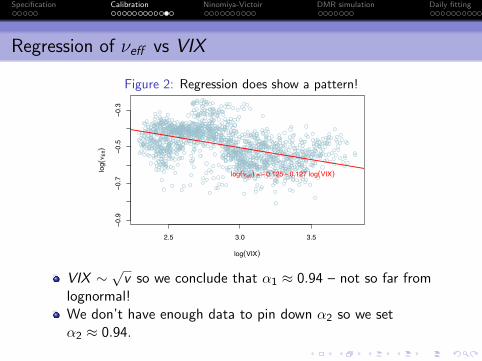
Regression of νeff vs VIX

Figure 2: Regression does show a pattern!

2.5 3.0 3.5

−0.9

−0.7

−0.5

−0.3

log(VIX)

log (i E

ff)

log(ieff) = <0.125 < 0.127 log(VIX)

VIX ∼√

v so we conclude that α1 ≈ 0.94 – not so far fromlognormal!We don’t have enough data to pin down α2 so we setα2 ≈ 0.94.


Daily calibration of remaining parameters

Although the volatility of volatility parameters ξ1 and ξ2 are inprinciple constants of the DMR model, it is clear fromFigure 1 that they are not constant in the data.

And of course, VIX option prices fluctuate from day to day.The implied volatility of VIX options is like volatility ofvolatility.

This leads to the following daily procedure:1 Calibrate vt and v ′t to variance swaps (from SPX option prices)

using linear regression.2 Calibrate ξ1 and ξ2 to VIX options data.3 Calibrate the correlations ρ12 and ρ13 to the SPX volatility

surface.

In steps 2 and 3, we need to use numerical techniques tocompute VIX and SPX options prices respectively.


The LKV scheme

In [my Bachelier 2008 presentation], calibration of ξ1, ξ2, ρ12

and ρ13 was performed using Monte-Carlo simulation.

The chosen scheme was Euler-Maruyama with partialtruncation as in [Lord, Koekkoek, and van Dijk]:

x((k + 1)∆) = −1

2v(k∆)∆ +

√v(k∆)Z 1

k

v((k + 1)∆) = v(k∆) + κ2 (v ′(k∆)− v(k∆)) ∆ +(v(k∆)+

)α1 Z 2k

v ′((k + 1)∆) = v ′(k∆) + κ2 (θ − v ′(k∆)) ∆ +(v ′(k∆)+

)α2 Z 3k .

In the above, ∆ is the time step, v(k∆) = v(k∆)+,v ′(k∆) = v ′(k∆)+, x(k∆) = log(S(k∆)), Z i

k ∼ N(0,∆) and

E[Z ik Z j

k ] = ρij ∆.

Calibration of the DMR model with this scheme is slow!


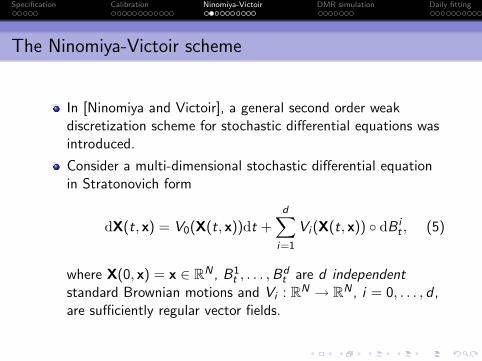
The Ninomiya-Victoir scheme

In [Ninomiya and Victoir], a general second order weakdiscretization scheme for stochastic differential equations wasintroduced.

Consider a multi-dimensional stochastic differential equationin Stratonovich form

dX(t, x) = V0(X(t, x))dt +d∑

i=1

Vi (X(t, x)) ◦ dB it , (5)

where X(0, x) = x ∈ RN , B1t , . . . ,B

dt are d independent

standard Brownian motions and Vi : RN → RN , i = 0, . . . , d ,are sufficiently regular vector fields.


The Ninomiya-Victoir scheme

The Ninomiya-Victoir scheme is given by

X(NV )(0, x) = x,

X(NV )((k + 1)∆, x)

=

{e

∆2 V0 eZ 1

k V1 · · · eZ dk Vd e

∆2 V0X(NV ) (k∆, x) , Λk = −1,

e∆2 V0 eZ d

k Vd · · · eZ 1k V1 e

∆2 V0X(NV ) (k∆, x) , Λk = +1.

(6)

etV x ∈ RN denotes the solution at time t ∈ R to the ODE

y = V (y) , y (0) = x,

i.e. the flow of the vector field.

The Λk take values ±1 with probability 1/2, the Z jk are

independent N (0,∆) random variables.


Features of the Ninomiya-Victoir scheme

One step in the NV scheme corresponds to a (non-discrete)cubature formula of order m = 5 in the sense of[Lyons and Victoir].

One can also interpret the NV scheme as the stochasticversion of a classical operator splitting scheme, where theinfinitesimal generator L = V0 + 1

2

∑di=1 V 2

i of the diffusion issplit into the first order differential operator V0 and thesecond order differential operators 1

2 V 21 , . . . , 1

2 V 2d .

The NV scheme is now widely used in applications such asInria’s software PREMIA for financial option computations.

In particular, a variant of the NV scheme due to [Alfonsi] canbe used to simulate the Heston model.


Solving the ODEs

Cubature methods, and the Ninomiya-Victoir scheme inparticular, need us to solve ODEs quickly and accurately.

General cubature methods involve ODEs with a rathercomplicated structure, involving all vector-fields at all times.

Numerical ODE methods such as Runge-Kutta are typicallyrequired.

If we are very lucky, all of the ODE flows may be solvedexactly – in terms of easy-to-evaluate expressions.

In such a case, one has effectively found a second order weakapproximation method which can be implemented withoutrelying on numerical ODE solvers

The Ninomiya-Victoir method can be expected to performespecially well in such cases.


The Drift Trick

The Heston model is one of the lucky cases where all of theODEs may be solved in closed form.

However, one soon encounters models where the ODEs haveno closed-form solution

For example, the SABR model.

[Bayer, Friz, and Loeffen] observed that the class of favorablemodels can be significantly enlarged by working with analmost trivial modification of the NV scheme.


The idea of the Drift Trick

We can rewrite the SDE as

dX(t, x) =

V0(X(t, x))−d∑

j=1

γj Vj (X(t, x))

dt

+d∑

j=1

Vj (X(t, x)) ◦ d(

B jt + γj t

)

=:V(γ)0 (X(t, x)) dt +

d∑j=1

Vj (X(t, x)) ◦ d(

B jt + γj t

)whatever the choice of drift parameters γ1, . . . , γd .In many cases of interest, it’s possible to choose the γi so asto permit the solution of all ODEs in closed-form.

In particular, the DMR model with α1 = α2 = 1, the DoubleLognormal model.


The NV scheme with drift trick

The Ninomiya-Victoir scheme with drift trick is now given by

XNVd) (0, x) = x,

X(NVd) ((k + 1)∆, x) ={e

∆2 V

(γ)0 eZ 1


∆2 V

(γ)0 X(NVd) (k∆, x) , Λk = −1,

e∆2 V

(γ)0 eZ d

k Vd · · · eZ 1k V1 e

∆2 V

(γ)0 X(NVd) (k∆, x) , Λk = +1,

(7)

where the Z ik ∼ N (∆γi ,∆) are again independent of each other.

This amended scheme corresponds to splitting L according to

L = V0 +1

2

d∑i=1

V 2i = V

(γ)0 +

d∑i=1

{1

2V 2

i + γi Vi

}.


More operator splitting

In models such as the DMR model with α1, α2 6= 1, the drifttrick is not enough to permit closed-form solution of the driftODE.

We may then try to find vector fields V0,1 and V0,2 such thatV0 = V0,1 + V0,2 and the ODEs driven by V0,1 and V0,2 have(closed-form) solutions etV0,1 and etV0,2 , respectively.

In that case, the solution e∆V0 of the ODE driven by thevector field V0 at time ∆ can be approximated by

e∆V0x = e∆V0,2e∆V0,1x +O(∆2),

a method sometimes known as the symplectic Euler scheme.

One contribution of the present work is to show that the NVscheme can be further extended in this way whilst maintainingsecond order weak convergence.


Our modified Ninomiya Victoir (NVs) scheme

In our modification of the NV scheme, applying thesymplectic Euler scheme to the solution of the drift ODE, weiterate according to

X(NVs)((k + 1)∆, x) ={e

∆2 V0,1 e

∆2 V0,2 eZ 1


∆2 V0,2 e

∆2 V0,1X(NVs) (k∆, x) , Λk = −1,

e∆2 V0,1 e

∆2 V0,2 eZ d

k Vd · · · eZ 1k V1 e

∆2 V0,2 e

∆2 V0,1X(NVs) (k∆, x) , Λk = +1.

(8)

This modified NVs scheme again has second orderconvergence in the weak sense.

In the case of the DMR model with α1, α2 6= 1, this furthersplitting of the drift operator V0 is sufficient to permit us tosolve all of the ODEs in closed form.


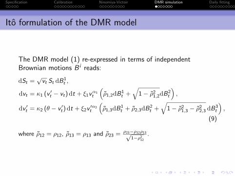
Ito formulation of the DMR model

The DMR model (1) re-expressed in terms of independentBrownian motions B i reads:

dSt =√

vt St dB1t ,

dvt = κ1 (v ′t − vt) dt + ξ1vα1t

(ρ1,2dB1

t +√

1− ρ21,2dB2

t

),

dv ′t = κ2 (θ − v ′t ) dt + ξ2v ′α2t

(ρ1,3dB1

t + ρ2,3dB2t +

√1− ρ2

1,3 − ρ22,3 dB3

t

),

(9)

where ρ12 = ρ12, ρ13 = ρ13 and ρ23 = ρ23−ρ12ρ13√1−ρ2

12

.


Stratonovich formulation of the DMR model

To apply NVs, we need the Stratonovich formulation:

X(t, x) = x +

∫ t

0V0 (X(s, x)) ds +

3∑j=1

∫ t

0Vj (X(s, x)) ◦ dB j

s

(10)where the state vector X(t, x) = (St , vt , v

′t)T , and the initial

condition is x = (S0, v0, v′0)T .

The driving vector fields {V0,V1,V2,V3} are given explicitlyin the following slide.


Explicit expressions for the vector fields

We have

V0(x) =

−12

(12 ξ1 ρ1,2 x

α1− 12

2 x1 + x2 x1

)−κ1 (x2 − x3)− 1

2 ξ21 α1 x2α1−1

2

−κ2(x3 − θ)− 12 ξ

22 α2 x2α2−1

3

and also

V1(x) =(√

x2 x1 ρ1,2 ξ1 xα12 ρ1,3 ξ2 xα2

3

)T

V2(x) =(

0√

1− ρ21,2 ξ1 xα1

2 ρ2,3 ξ2 xα23

)T

V3(x) =(

0 0√

1− ρ21,3 − ρ2

2,3 ξ2 xα23

)T.


Solving the ODEs

In order to implement the NVs scheme, we thus need to solvethe ODEs

ddt

x(t) = Vi (x(t))

for all i ∈ {0, 1, 2, 3} and t ∈ R with some given boundarycondition.

It is relatively straightforward to solve the ODEs fori ∈ {1, 2, 3} in closed form.

Solving the ODEddt

x(t) = V0(x(t))

requires further splitting.


The flow of the Stratonovich drift vector field

To solve the ODE for i = 0, we write

V0 = V0,1 + V0,2

with

V0,1(x) =

−12 x2 x1

−κ1 (x2 − x3)−κ2 (x3 − θ)

,

V0,2(x) =

−14 ξ1 ρ1,2 x

α1− 12

2 x1

−12 ξ

21 α1 x2α1−1

2

−12 ξ

22 α2 x2α2−1

3

.

It is again straightforward to solve the corresponding ODEs inclosed form.


The double lognormal case: α1 = α2 = 1

In the Double Lognormal case with α1 = 1, α2 = 1, we mayapplying the drift trick to get closed-form ODE solutions.

Specifically, with

V γ0 = V0 − γ1V1 − γ2V2 − γ3V3,

and choosing

γ1 = −ξ1 ρ1,2,

γ2 = −κ1 + 1

2ξ21 + γ1 ρ1,2 ξ1

ξ1

√1− ρ2

1,2

,

γ3 = −κ2 + 1

2 ξ22 − ρ1,3 ξ2 γ1 − ρ2,3 ξ2 γ2

ξ2

√1− ρ2

1,3 − ρ22,3

,

we end up with much simpler expressions for the vector fields.


The adjusted drift vector field

Explicitly, after applying the drift trick, we get

V γ0 =

−12 x2 x1

κ1 x3

κ2 θ

which is much simpler than the original

V0(x) =

−12

(12 ξ1 ρ1,2

√x2 x1 + x2 x1

)−κ1 (x2 − x3)− 1

2 ξ21 x2

−κ2(x3 − θ)− 12 ξ

22 x3

It is again straightforward to compute solutions to theseODEs in closed-form.


Daily model fitting

Once again, the model parameters κ1, κ2, θ and ρ23 areconsidered fixed.

The state variables vt and v ′t are obtained by linear regressionagainst the fair values of variance swaps proxied by thelog-strip.

Arbitrage-free interpolation and extrapolation of the volatilitysurface is achieved using the SVI parameterization in[Gatheral and Jacquier].

The volatility-of-volatility parameters ξ1 and ξ2 are obtainedby calibrating the DMR model to the market prices of VIXoptions (using NVs).

The correlation parameters ρ12 and ρ13 are then calibrated toSPX options.


Pricing VIX options

The payoff of a call option on the VIX index with strike Kexpiring at time T may be written as√E

[∫ T +∆

Tvsds

∣∣∣∣ FT

]− K

+

where ∆ is is roughly one month.

Each Monte Carlo path generates a value for vT and v ′T , so

the expected forward variance E[∫ T +∆

T vsds∣∣∣ FT

]is given

by equation (3).

Averaging over all paths gives the model price of the VIXoption.


Calibration to VIX options

Our chosen objective function is the sum of squareddifferences between market VIX implied volatilities and modelVIX implied volatilities. Errors are weighted by the reciprocalof the bid-ask spread:√√√√∑

i

(σmid

i − σmodeli

σaski − σbid

i

)2

.


Calibration to SPX options

We are then left with the correlation parameters ρ12 and ρ13

to calibrate to the SPX volatility surface.

Note only two parameters to fit the entire volatility surface!

Our objective function is again the sum of squared differencesbetween market SPX implied volatilities and model SPXimplied volatilities, weighted by the reciprocal of the bid-askspread.


Two days in history

We pick two days in history to fit the DMR model, one beforethe 2008 financial crisis, and one after:

April 3, 2007 and September 15, 2011.

Recall that fixed model parameters were as follows:

θ 0.078κ1 5.5κ2 0.10ρ23 0.59α1 0.94α2 0.94


Fitted parameters

With vt , v ′t from variance swaps, ξ1, ξ2 from VIX options, andρ12, ρ13 from SPX options we obtain:

03-Apr-2007 15-Sep-2011

v 0.0153 0.114v ′ 0.0224 0.110ξ1 2.873 2.689ξ2 0.302 0.502ρ12 -0.992 -0.982ρ13 -0.615 -0.727

Note that fitted parameters from two very different marketenvironments are very similar.


Variance swap fit as of April 3, 2007

0.0 0.5 1.0 1.5 2.0 2.5 3.0

0.01

50.

020

0.02

50.

030

Maturity

Var

sw

ap

●

●

●

●●

●● ●

●●●

●

●

●

Figure 3: The points are SPX variance swaps (from the log-strip), the solidcurve is the DMR model fit.


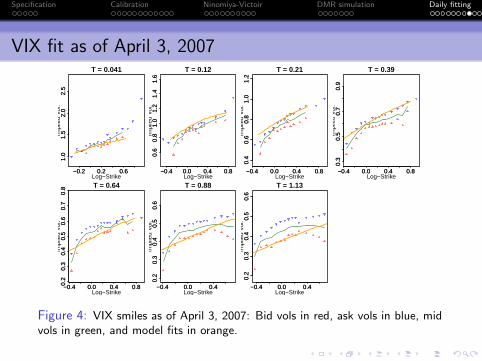
VIX fit as of April 3, 2007

−0.2 0.2 0.6

1.0

1.5

2.0

2.5

T = 0.041

Log−Strike

Impl

ied

Vol

.

−0.2 0.2 0.6

1.0

1.5

2.0

2.5

−0.4 0.0 0.4 0.8

0.6

0.8

1.0

1.2

1.4

1.6

T = 0.12

Log−Strike

Impl

ied

Vol

.

−0.4 0.0 0.4 0.8

0.6

0.8

1.0

1.2

1.4

1.6

−0.4 0.0 0.4 0.8

0.4

0.6

0.8

1.0

1.2

T = 0.21

Log−Strike

Impl

ied

Vol

.

−0.4 0.0 0.4 0.8

0.4

0.6

0.8

1.0

1.2

−0.4 0.0 0.4 0.8

0.3

0.5

0.7

0.9

T = 0.39

Log−Strike

Impl

ied

Vol

.

−0.4 0.0 0.4 0.8

0.3

0.5

0.7

0.9

−0.4 0.0 0.4 0.80.2

0.3

0.4

0.5

0.6

0.7

0.8 T = 0.64

Log−Strike

Impl

ied

Vol

.

−0.4 0.0 0.4 0.80.2

0.3

0.4

0.5

0.6

0.7

0.8

−0.4 0.0 0.4

0.2

0.3

0.4

0.5

0.6

T = 0.88

Log−Strike

Impl

ied

Vol

.

−0.4 0.0 0.4

0.2

0.3

0.4

0.5

0.6

−0.4 0.0 0.4

0.2

0.3

0.4

0.5

0.6

T = 1.13

Log−Strike

Impl

ied

Vol

.

−0.4 0.0 0.4

0.2

0.3

0.4

0.5

0.6

Figure 4: VIX smiles as of April 3, 2007: Bid vols in red, ask vols in blue, midvols in green, and model fits in orange.


SPX fit as of April 3, 2007

−0.06 −0.02

0.0

0.2

0.4

T = 0.0055

Log−Strike

Impl

ied

Vol

.

−0.06 −0.02

0.0

0.2

0.4

−0.5 −0.2 0.0

0.0

0.4

0.8

T = 0.049

Log−Strike

Impl

ied

Vol

.

−0.5 −0.2 0.0

0.0

0.4

0.8

−0.5 −0.2 0.0

0.1

0.3

0.5

T = 0.13

Log−Strike

Impl

ied

Vol

.

−0.5 −0.2 0.0

0.1

0.3

0.5

−0.8 −0.4 0.0

0.0

0.4

T = 0.20

Log−Strike

Impl

ied

Vol

.

−0.8 −0.4 0.0

0.0

0.4

−0.10 0.000.05

0.15

T = 0.24

Log−Strike

Impl

ied

Vol

.

−0.10 0.000.05

0.15

−0.6 −0.2

0.1

0.3

T = 0.47

Log−Strike

Impl

ied

Vol

.

−0.6 −0.2

0.1

0.3

−0.10 0.00

0.10

0.20

T = 0.49

Log−Strike

Impl

ied

Vol

.

−0.10 0.00

0.10

0.20

−0.8 −0.4 0.0

0.1

0.3

T = 0.72

Log−Strike

Impl

ied

Vol

.

−0.8 −0.4 0.0

0.1

0.3

−0.10 0.00

0.08

0.14

0.20

T = 0.74

Log−Strike

Impl

ied

Vol

.

−0.10 0.00

0.08

0.14

0.20

−0.4 −0.2 0.0

0.10

0.20

T = 0.97

Log−Strike

Impl

ied

Vol

.

−0.4 −0.2 0.0

0.10

0.20

−0.20 −0.05 0.05

0.10

0.16

0.22

T = 0.99

Log−Strike

Impl

ied

Vol

.

−0.20 −0.05 0.05

0.10

0.16

0.22

−0.6 −0.3 0.0

0.10

0.20

0.30

T = 1.22

Log−Strike

Impl

ied

Vol

.

−0.6 −0.3 0.0

0.10

0.20

0.30

−0.8 −0.4 0.0

0.10

0.20

0.30

T = 1.72

Log−Strike

Impl

ied

Vol

.

−0.8 −0.4 0.0

0.10

0.20

0.30

−0.8 −0.4 0.0

0.10

0.20

0.30

T = 2.71

Log−Strike

Impl

ied

Vol

.

−0.8 −0.4 0.0

0.10

0.20

0.30


VIX fit as of September 15, 2011

−1.0 −0.5 0.0 0.5 1.0

12

34

5T = 0.016

Log−Strike

Impl

ied

Vol

.

−1.0 −0.5 0.0 0.5 1.0

12

34

5

−1.0 −0.5 0.0 0.5 1.0

1.0

1.5

2.0

T = 0.093

Log−StrikeIm

plie

d V

ol.

−1.0 −0.5 0.0 0.5 1.0

1.0

1.5

2.0

−1.0 −0.5 0.0 0.5 1.0

0.6

0.8

1.0

1.2

1.4

1.6 T = 0.17

Log−Strike

Impl

ied

Vol

.

−1.0 −0.5 0.0 0.5 1.0

0.6

0.8

1.0

1.2

1.4

1.6

−1.0 −0.5 0.0 0.5 1.0

0.4

0.6

0.8

1.0

1.2

T = 0.27

Log−Strike

Impl

ied

Vol

.

−1.0 −0.5 0.0 0.5 1.0

0.4

0.6

0.8

1.0

1.2

−1.0 −0.5 0.0 0.5 1.0

0.4

0.6

0.8

1.0

1.2

T = 0.34

Log−Strike

Impl

ied

Vol

.

−1.0 −0.5 0.0 0.5 1.0

0.4

0.6

0.8

1.0

1.2

−1.0 −0.5 0.0 0.5 1.0

0.4

0.6

0.8

1.0

1.2 T = 0.42

Log−Strike

Impl

ied

Vol

.

−1.0 −0.5 0.0 0.5 1.0

0.4

0.6

0.8

1.0

1.2

Figure 5: VIX smiles as of September 15, 2011: Bid vols in red, ask vols inblue, and model fits in orange. Note that the fitted smiles seem a little too flat.


SPX fit as of September 15, 2011

−2.5 −1.0 0.0 1.0

04

812

T = 0.0027

Log−Strike

Impl

ied

Vol

.

−2.5 −1.0 0.0 1.0

04

812

−0.2 0.0 0.1

0.2

0.4

0.6

0.8

T = 0.019

Log−Strike

Impl

ied

Vol

.

−0.2 0.0 0.1

0.2

0.4

0.6

0.8

−0.8 −0.4 0.0

0.5

1.0

1.5

T = 0.038

Log−Strike

Impl

ied

Vol

.

−0.8 −0.4 0.0

0.5

1.0

1.5

−2.5 −1.5 −0.5

0.0

1.0

2.0

3.0

T = 0.099

Log−Strike

Impl

ied

Vol

.

−2.5 −1.5 −0.5

0.0

1.0

2.0

3.0

−2.5 −1.5 −0.5

0.0

1.0

2.0

T = 0.18

Log−Strike

Impl

ied

Vol

.

−2.5 −1.5 −0.5

0.0

1.0

2.0

−3 −2 −1 0 1

0.0

1.0

2.0

T = 0.25

Log−Strike

Impl

ied

Vol

.

−3 −2 −1 0 1

0.0

1.0

2.0

−0.6 −0.2 0.2

0.1

0.3

0.5

0.7

T = 0.29

Log−Strike

Impl

ied

Vol

.

−0.6 −0.2 0.2

0.1

0.3

0.5

0.7

−1.5 −0.5

0.2

0.6

1.0

T = 0.50

Log−Strike

Impl

ied

Vol

.

−1.5 −0.5

0.2

0.6

1.0

−0.4 0.0 0.40.1

0.3

0.5

T = 0.54

Log−Strike

Impl

ied

Vol

.

−0.4 0.0 0.40.1

0.3

0.5

−2.5 −1.0 0.0 1.0

0.2

0.6

1.0

T = 0.75

Log−Strike

Impl

ied

Vol

.

−2.5 −1.0 0.0 1.0

0.2

0.6

1.0

−0.6 −0.2 0.2

0.2

0.4

0.6 T = 0.79

Log−Strike

Impl

ied

Vol

.

−0.6 −0.2 0.2

0.2

0.4

0.6

−2.5 −1.0 0.0 1.0

0.2

0.6

T = 1.27

Log−Strike

Impl

ied

Vol

.

−2.5 −1.0 0.0 1.0

0.2

0.6

−2.5 −1.5 −0.5 0.5

0.2

0.6

T = 1.77

Log−Strike

Impl

ied

Vol

.

−2.5 −1.5 −0.5 0.5

0.2

0.6

−2.5 −1.0 0.0 1.0

0.0

0.4

0.8

T = 2.26

Log−Strike

Impl

ied

Vol

.

−2.5 −1.0 0.0 1.0

0.0

0.4

0.8


Double Lognormal model calibration to 2011 data

In Figure , we saw that the DMR model with α1 = α2 = 0.94generates VIX option smiles that are too flat.

This motivates us to calibrate the simpler Double Lognormalversion of the DMR model with α1 = α2 = 1.

Simulation is also faster because we use the drift trick. Eachtime step is less complex.


VIX fit of Double Lognormal as of September 15, 2011

−1.0 −0.5 0.0 0.5 1.0

12

34

5T = 0.016

Log−Strike

Impl

ied

Vol

.

−1.0 −0.5 0.0 0.5 1.0

12

34

5

−1.0 −0.5 0.0 0.5 1.0

1.0

1.5

2.0

T = 0.093

Log−StrikeIm

plie

d V

ol.

−1.0 −0.5 0.0 0.5 1.0

1.0

1.5

2.0

−1.0 −0.5 0.0 0.5 1.0

0.6

0.8

1.0

1.2

1.4

1.6 T = 0.17

Log−Strike

Impl

ied

Vol

.

−1.0 −0.5 0.0 0.5 1.0

0.6

0.8

1.0

1.2

1.4

1.6

−1.0 −0.5 0.0 0.5 1.0

0.4

0.6

0.8

1.0

1.2

T = 0.27

Log−Strike

Impl

ied

Vol

.

−1.0 −0.5 0.0 0.5 1.0

0.4

0.6

0.8

1.0

1.2

−1.0 −0.5 0.0 0.5 1.0

0.4

0.6

0.8

1.0

1.2

T = 0.34

Log−Strike

Impl

ied

Vol

.

−1.0 −0.5 0.0 0.5 1.0

0.4

0.6

0.8

1.0

1.2

−1.0 −0.5 0.0 0.5 1.0

0.4

0.6

0.8

1.0

1.2 T = 0.42

Log−Strike

Impl

ied

Vol

.

−1.0 −0.5 0.0 0.5 1.0

0.4

0.6

0.8

1.0

1.2

Figure 6: VIX smiles as of September 15, 2011: Bid vols in red, ask vols inblue, and Double Lognormal model fits in orange.


Remarks on the Double Lognormal fit

The smiles got a little steeper.

The algorithm (with the drift trick) is less complex.

And the model with α1 = α2 = 1 is more parsimonious.

Double Lognormal seems like the better choice!


Performance tradeoff between NV and EM

The Ninomiya-Victoir (NV) scheme permits us to achieve agiven target RMSE with fewer time steps thanEuler-Maruyama (EM).However, the computational cost of each NV time step isgreater than EM.The tradeoff between NV and EM must therefore be assessedexperimentally.

2D 3D

α1 = α2 = 0.94 4.55 6.84

α1 = α2 = 1 1.81 3.08

Table 1: Relative computation times for NV steps in terms of EM steps. 2Dmeans simulation of the variance process only (i.e. for VIX options); 3D meanssimulation of the full model. The values are obtained by simulating with 90time steps and 218 QMC paths using the parameters obtained in the 2011calibrations.


Optimal calibration recipe

From experiment, we conclude that it is better to use the EMdiscretization when calibrating to SPX options where there islittle if any RMSE reduction benefit from using the NV step.

However, for VIX options, we can achieve a speedup of 3− 4times in the 2007 example, 2 in the 2011 example and 5 inthe 2011 lognormal DMR example.

The optimal calibration recipe appears to be:

Calibrate ξ1 and ξ2 with a Ninomiya-Victoir scheme.Calibrate ρ12 and ρ13 with an Euler-Maruyama scheme.

Using Java code with 30 time steps and 211 paths we cantypically calibrate the model to both SPX and VIX optionmarkets in less than 5 seconds.


Conclusion

We have presented two straightforward modifications of thestandard Ninomiya-Victoir discretization scheme that conservesecond order weak convergence but permit simple closed-formsolutions to the ODE’s.

NV with drift trick, and NV with extra splitting of the driftvector field.

Using these schemes for VIX options and the simplerEuler-Maruyama scheme for SPX options, we demonstratedthat it is possible to achieve fast and accurate calibration ofthe DMR model to both SPX and VIX options marketssimultaneously.Moreover, we demonstrated that the DMR model fits SPXand VIX options market data well for two particular dateschosen to represent two very different market environmentsfrom before and after the 2008 financial crisis.

The fitted parameters of the model over time appear to beremarkably stable.


References

Aurelien Alfonsi, High order discretization schemes for the CIR process: Application to affine term structure

and Heston models, Mathematics of Computation 79(269) 209–237 (2010).

Christian Bayer, Peter Friz, and Ronnie Loeffen, Semi-closed form cubature and applications to financial

diffusion models, Quantitative Finance 13(5), 769–782 (2013).

Christian Bayer, Jim Gatheral, and Morten Karlsmark, Fast Ninomiya-Victoir calibration of the

double-mean-reverting model, Quantitative Finance forthcoming (2013).

Jim Gatheral, The Volatility Surface: A Practitioner’s Guide, John Wiley and Sons, Hoboken, NJ (2006).

Jim Gatheral, Consistent Modeling of SPX and VIX Options, Fifth World Congress of the Bachelier Finance

Society (2008).

Jim Gatheral and Antoine Jacquier, Arbitrage-free SVI volatility surfaces, Quantitative Finance forthcoming

(2013).

Patrick Hagan, Deep Kumar, Andrew Lesniewski, and Diana Woodward, Managing smile risk, Wilmott

Magazine 1/(1) 84–108 (2002).

Roger Lord, Koekkoek, and D. van Dijk, A comparison of biased simulation schemes for stochastic volatility

models Quantitative Finance 10(2) 177–194 (2010).

Terry Lyons and Nicolas Victoir, Cubature on Wiener space, Proc. R. Soc. Lond. Ser. A Math. Phys. Eng.

Sci. 460(2041) 169–198 (2004).

Syoiti Ninomiya and Nicolas Victoir, Weak approximation of stochastic differential equations and

application to derivative pricing, Applied Mathematical Finance 15 107–121 (2008).

Fast Ninomiya-Victoir calibration of ... - … cation Calibration Ninomiya-Victoir DMR simulation...

Documents

Transcript of Fast Ninomiya-Victoir calibration of ... - … cation Calibration Ninomiya-Victoir DMR simulation...