Fast Marching Methods for Front Propagation Lecture...
77
Outline Fast Marching Methods for Front Propagation Lecture 1/3 M. Falcone Dipartimento di Matematica SAPIENZA, Universit` a di Roma Autumn School ”Introduction to Numerical Methods for Moving Boundaries” ENSTA, Paris, November, 12-14, 2007 M. Falcone Fast Marching Methods for Front Propagation
Transcript of Fast Marching Methods for Front Propagation Lecture...
Outline
Fast Marching Methods for Front Propagation
Lecture 1/3
M. Falcone
Dipartimento di MatematicaSAPIENZA, Universita di Roma
Autumn School”Introduction to Numerical Methods for Moving Boundaries”
ENSTA, Paris, November, 12-14, 2007
M. Falcone Fast Marching Methods for Front Propagation
Outline
Outline
1 Introduction
2 Front Propagation and Minimum Time Problem
3 Global Numerical Approximations
4 Fast Marching MethodsA CFL-like condition for FM method
M. Falcone Fast Marching Methods for Front Propagation

IntroductionFront Propagation and Minimum Time Problem
Global Numerical ApproximationsFast Marching Methods
Level Set Method
The Level Set method has had a great success for the analysis offront propagation problems for its capability to handle manydifferent physical phenomena within the same theoreticalframework.One can use it for isotropic and anisotropic front propagation, formerging different fronts, for Mean Curvature Motion (MCM) andother situations when the velocity depends on some geometricalproperties of the front.It allows to develop the analysis also after the on set ofsingularities.
M. Falcone Fast Marching Methods for Front Propagation
IntroductionFront Propagation and Minimum Time Problem
Global Numerical ApproximationsFast Marching Methods
Level Set Method
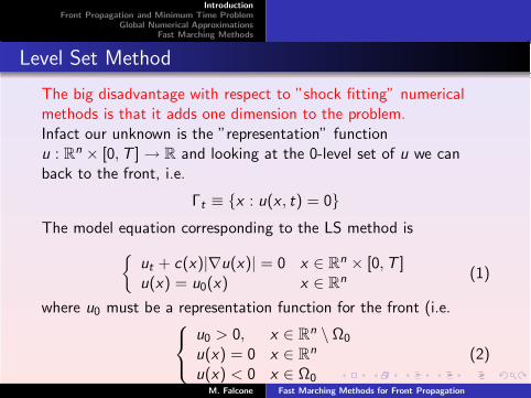
The big disadvantage with respect to ”shock fitting” numericalmethods is that it adds one dimension to the problem.Infact our unknown is the ”representation” functionu : R
n × [0,T ] → R and looking at the 0-level set of u we canback to the front, i.e.
Γt ≡ x : u(x , t) = 0The model equation corresponding to the LS method is
ut + c(x)|∇u(x)| = 0 x ∈ R
n × [0,T ]u(x) = u0(x) x ∈ R
n (1)
where u0 must be a representation function for the front (i.e.
u0 > 0, x ∈ Rn \ Ω0
u(x) = 0 x ∈ Rn
u(x) < 0 x ∈ Ω0
(2)
M. Falcone Fast Marching Methods for Front Propagation
IntroductionFront Propagation and Minimum Time Problem
Global Numerical ApproximationsFast Marching Methods
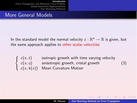
More General Models
In the standard model the normal velocity c : Rn → R is given, but
the same approach applies to other scalar velocities
c(x , t) isotropic growth with time varying velocityc(x , η) anisotropic growth, cristal growthc(x , k(x)) Mean Curvature Motion
(3)
M. Falcone Fast Marching Methods for Front Propagation
IntroductionFront Propagation and Minimum Time Problem
Global Numerical ApproximationsFast Marching Methods
Fast Marching Method
In this process we do not want loose accuracy and we would like tokeep the derivative of u big enough (ideally |Du(x)| = 1) to get anaccurate representation of the front (re-initialization).
The Fast Marching method has been conceived to speed up thecomputations and save CPU time.
The crucial point is to concentrate the computational effort aroundthe front at every iteration avoiding useless computations.
M. Falcone Fast Marching Methods for Front Propagation

IntroductionFront Propagation and Minimum Time Problem
Global Numerical ApproximationsFast Marching Methods
Questions
In order to set up and analyze the FMM we have to answer severalquestions:
what is the initial configuration of the front in our numericalscheme?
what is the position of the front at every iteration?
which nodes will be necessary to compute the frontconfiguration at the following time step?
does the procedure converge to the correct viscosity solution?
how many operations will be needed to get the right solution?
M. Falcone Fast Marching Methods for Front Propagation

IntroductionFront Propagation and Minimum Time Problem
Global Numerical ApproximationsFast Marching Methods
Outline
1 Introduction
2 Front Propagation and Minimum Time Problem
3 Global Numerical Approximations
4 Fast Marching MethodsA CFL-like condition for FM method
M. Falcone Fast Marching Methods for Front Propagation

IntroductionFront Propagation and Minimum Time Problem
Global Numerical ApproximationsFast Marching Methods
Monotone evolution of fronts
Assume that the sign of the normal velocity is fixed, f.e. takec(x) > 0.The evolution of the front is monotone increasing in the sense thatthe measure of the domain entoured by the front Γt is increasing.Defining
Ωt ≡ x : u(x , t) < 0this means that Ωt ⊂ Ωt+s for every s > 0.If the evolution of the front is monotone we have an interestinglink with the minimum time problem.
M. Falcone Fast Marching Methods for Front Propagation
IntroductionFront Propagation and Minimum Time Problem
Global Numerical ApproximationsFast Marching Methods
The minimum time problem
Let us consider the nonlinear system
y(t) = f (y(t), a(t)), t > 0,y(0) = x
(D)
wherey(t) ∈ R
N is the statea( · ) ∈ A is the control
A = admissible control functions
= a : [0,+∞[ → A, measurable
(e.g. A = piecewise constant functions with values in A),
M. Falcone Fast Marching Methods for Front Propagation
IntroductionFront Propagation and Minimum Time Problem
Global Numerical ApproximationsFast Marching Methods
The model problem
A ⊂ RM is a given compact set.
Assume f is continuous and
|f (x , a) − f (y , a)| ≤ L |x − y | ∀x , y ∈ RN , a ∈ A.
Then, for each a( · ) ∈ A, there is a uniquetrajectory of (D), yx(t; a, b) (Caratheodory Theorem).
M. Falcone Fast Marching Methods for Front Propagation
IntroductionFront Propagation and Minimum Time Problem
Global Numerical ApproximationsFast Marching Methods
Payoff
The payoff of the Minimum Time Problem is
tx(a( · )) = min t : yx(t; a) ∈ T ≤ +∞,
where T ⊆ RN is a given closed target.
GoalWe want to minimize the payoff, i.e. the time to transfer thesystem from its initial position x to the target T . The valuefunction is
T (x) ≡ infa( · )∈A
tx(a) .
( T is the minimum time function).
M. Falcone Fast Marching Methods for Front Propagation
IntroductionFront Propagation and Minimum Time Problem
Global Numerical ApproximationsFast Marching Methods
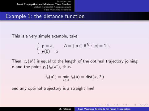
Example 1: the distance function
This is a very simple example, take
y = a, A = a ∈ R
N : |a| = 1 ,y(0) = x .
Then, tx(a∗) is equal to the length of the optimal trajectory joining
x and the point yx(tx(a∗), thus
tx(a∗) = min
a∈Atx(a) = dist(x ,T )
and any optimal trajectory is a straight line!
M. Falcone Fast Marching Methods for Front Propagation
IntroductionFront Propagation and Minimum Time Problem
Global Numerical ApproximationsFast Marching Methods
Reachable set
Definition
R ≡ x ∈ RN : T (x) < +∞, i.e. the set of starting points from
which it is possible to reach the target (a priori this can be empty).
WARNINGThe reachable set R depends on the target and on the dynamics ina rather complicated way. It is NOT a datum in our problem.
M. Falcone Fast Marching Methods for Front Propagation

IntroductionFront Propagation and Minimum Time Problem
Global Numerical ApproximationsFast Marching Methods
Dynamic Programming
Lemma (Dynamic Programming Principle)
For all x ∈ R, 0 ≤ t < T (x) (so that x /∈ T ),
T (x) = infa( · )∈A
t + T (yx(t; a)) . (DPP)
“Proof”The inequality “≤” follows from the intuitive fact that ∀a( · )
T (x) ≤ t + T (yx(t; a)).
M. Falcone Fast Marching Methods for Front Propagation

IntroductionFront Propagation and Minimum Time Problem
Global Numerical ApproximationsFast Marching Methods
DP Principle
The proof of the opposite inequality “≥” is based on the fact thatthe equality holds if a( · ) is optimal for x .For any ε > 0 we can find a minimizing control aε such that
T (x) + ε ≥ t + T (yx(t; aε)
split the trajectory and pass to the limit for ε → 0.
M. Falcone Fast Marching Methods for Front Propagation

IntroductionFront Propagation and Minimum Time Problem
Global Numerical ApproximationsFast Marching Methods
Sketch of the proof
To prove rigorously the above inequalities the following twoproperties of A are crucial:
1 a( · ) ∈ A ⇒ ∀s ∈ R the function t 7→ a(t + s) is in A;
2 a1, a2 ∈ A ⇒ a( · ) ∈ A ∀s > 0, where
a(t) ≡
a1(t) t ≤ s,a2(t) t > s.
M. Falcone Fast Marching Methods for Front Propagation

IntroductionFront Propagation and Minimum Time Problem
Global Numerical ApproximationsFast Marching Methods
Note that the DPP works for
A = piecewise constants functions into A
but not for
A = continuous functions into A .
because joining together two continuous controls we are notguaranteed that the resulting control is continuous.
M. Falcone Fast Marching Methods for Front Propagation
IntroductionFront Propagation and Minimum Time Problem
Global Numerical ApproximationsFast Marching Methods
Bellman equation
Let us derive the Hamilton-Jacobi-Bellman equation from the DPP.Rewrite (DPP) as
T (x) − infa( · )
T (yx(t; a)) = t
and divide by t > 0,
supa( · )
T (x) − T (yx(t; a))
t
= 1 ∀t < T (x) .
We want to pass to the limit as t → 0+.
M. Falcone Fast Marching Methods for Front Propagation
IntroductionFront Propagation and Minimum Time Problem
Global Numerical ApproximationsFast Marching Methods
Bellman equation
Assume T is differentiable at x and limt→0+ commute withsupa( · ). Then, if yx(0; a) exists,
supa( · )∈A
−∇T (x) · yx(0, a) = 1,
and then, if limt→0+
a(t) = a0, we get
supa0∈A
−∇T (x) · f (x , a0) = 1 . (HJB)
This is the Hamilton-Jacobi-Bellman partial differential equation(first order, fully nonlinear PDE).
M. Falcone Fast Marching Methods for Front Propagation
IntroductionFront Propagation and Minimum Time Problem
Global Numerical ApproximationsFast Marching Methods
Bellman equation
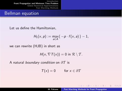
Let us define the Hamiltonian,
H1(x , p) := maxa∈A
−p · f (x , a) − 1,
we can rewrite (HJB) in short as
H(x ,∇T (x)) = 0 in R \ T .
A natural boundary condition on ∂T is
T (x) = 0 for x ∈ ∂T
M. Falcone Fast Marching Methods for Front Propagation
IntroductionFront Propagation and Minimum Time Problem
Global Numerical ApproximationsFast Marching Methods
T verifies the HJB equation
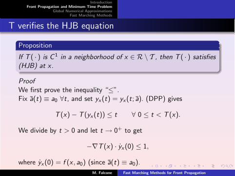
Proposition
If T ( · ) is C 1 in a neighborhood of x ∈ R \ T , then T ( · ) satisfies(HJB) at x.
ProofWe first prove the inequality “≤”.Fix a(t) ≡ a0 ∀t, and set yx(t) = yx(t; a). (DPP) gives
T (x) − T (yx(t)) ≤ t ∀ 0 ≤ t < T (x).
We divide by t > 0 and let t → 0+ to get
−∇T (x) · yx(0) ≤ 1,
where yx(0) = f (x , a0) (since a(t) ≡ a0).
M. Falcone Fast Marching Methods for Front Propagation

IntroductionFront Propagation and Minimum Time Problem
Global Numerical ApproximationsFast Marching Methods
T verifies the HJB equation
Then,−∇T (x) · f (x , a0) ≤ 1 ∀a0 ∈ A
and we getmaxa∈A
−∇T (x) · f (x , a) ≤ 1 .
Next we prove the inequality “≥”.
M. Falcone Fast Marching Methods for Front Propagation
IntroductionFront Propagation and Minimum Time Problem
Global Numerical ApproximationsFast Marching Methods
T verifies the HJB equation
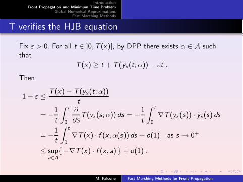
Fix ε > 0. For all t ∈ ]0,T (x)[, by DPP there exists α ∈ A suchthat
T (x) ≥ t + T (yx(t;α)) − εt .
Then
1 − ε ≤ T (x) − T (yx(t;α))
t
= −1
t
∫ t
0
∂
∂sT (yx(s;α)) ds = −1
t
∫ t
0∇T (yx(s)) · yx(s) ds
= −1
t
∫ t
0∇T (x) · f (x , α(s)) ds + o(1) as s → 0+
≤ supa∈A
−∇T (x) · f (x , a) + o(1) .
M. Falcone Fast Marching Methods for Front Propagation
IntroductionFront Propagation and Minimum Time Problem
Global Numerical ApproximationsFast Marching Methods
T verifies the HJB equation
Letting s → 0+, ε → 0+ we get
supa∈A
−∇T (x) · f (x , a) ≥ 1 .
We have proved that if T is regular then it satisfies (pointwise) theBellman equation in the reachable set R
M. Falcone Fast Marching Methods for Front Propagation
IntroductionFront Propagation and Minimum Time Problem
Global Numerical ApproximationsFast Marching Methods
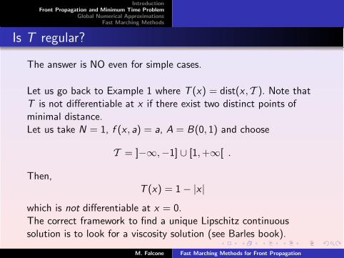
Is T regular?
The answer is NO even for simple cases.
Let us go back to Example 1 where T (x) = dist(x ,T ). Note thatT is not differentiable at x if there exist two distinct points ofminimal distance.Let us take N = 1, f (x , a) = a, A = B(0, 1) and choose
T = ]−∞,−1] ∪ [1,+∞[ .
Then,T (x) = 1 − |x |
which is not differentiable at x = 0.The correct framework to find a unique Lipschitz continuoussolution is to look for a viscosity solution (see Barles book).
M. Falcone Fast Marching Methods for Front Propagation
IntroductionFront Propagation and Minimum Time Problem
Global Numerical ApproximationsFast Marching Methods
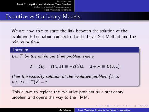
Evolutive vs Stationary Models
We are now able to state the link between the solution of theevolutive HJ equation connected to the Level Set Method and theminimum time
Theorem
Let T be the minimum time problem where
T = Ω0, f (x , a) ≡ −c(x)a, a ∈ A ≡ B(0, 1)
then the viscosity solution of the evolutive problem (1) isu(x , t) = T (x) − t.
This allows to replace the evolutive problem by a stationaryproblem and opens the way to the FMM.
M. Falcone Fast Marching Methods for Front Propagation

IntroductionFront Propagation and Minimum Time Problem
Global Numerical ApproximationsFast Marching Methods
Outline
1 Introduction
2 Front Propagation and Minimum Time Problem
3 Global Numerical Approximations
4 Fast Marching MethodsA CFL-like condition for FM method
M. Falcone Fast Marching Methods for Front Propagation
IntroductionFront Propagation and Minimum Time Problem
Global Numerical ApproximationsFast Marching Methods
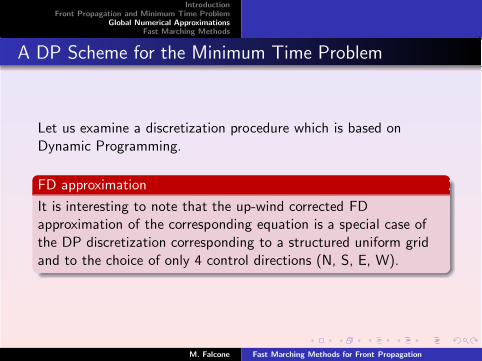
A DP Scheme for the Minimum Time Problem
Let us examine a discretization procedure which is based onDynamic Programming.
FD approximation
It is interesting to note that the up-wind corrected FDapproximation of the corresponding equation is a special case ofthe DP discretization corresponding to a structured uniform gridand to the choice of only 4 control directions (N, S, E, W).
M. Falcone Fast Marching Methods for Front Propagation
IntroductionFront Propagation and Minimum Time Problem
Global Numerical ApproximationsFast Marching Methods
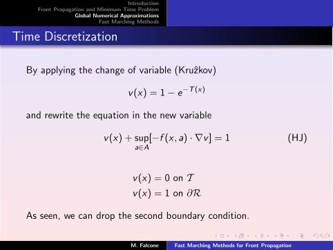
Time Discretization
By applying the change of variable (Kruzkov)
v(x) = 1 − e−T (x)
and rewrite the equation in the new variable
v(x) + supa∈A
[−f (x , a) · ∇v ] = 1 (HJ)
v(x) = 0 on Tv(x) = 1 on ∂R
As seen, we can drop the second boundary condition.
M. Falcone Fast Marching Methods for Front Propagation
IntroductionFront Propagation and Minimum Time Problem
Global Numerical ApproximationsFast Marching Methods
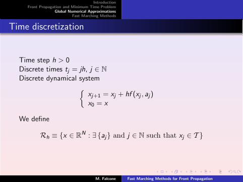
Time discretization
Time step h > 0Discrete times tj = jh, j ∈ N
Discrete dynamical system
xj+1 = xj + hf (xj , aj)x0 = x
We define
Rh ≡ x ∈ RN : ∃ aj and j ∈ N such that xj ∈ T
M. Falcone Fast Marching Methods for Front Propagation
IntroductionFront Propagation and Minimum Time Problem
Global Numerical ApproximationsFast Marching Methods
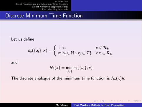
Discrete Minimum Time Function
Let us define
nh(aj, x) =
+∞ x /∈ Rh
min∈ N : xj ∈ T ∀ x ∈ Rh
andNh(x) = min
ajnh(aj, x)
The discrete analogue of the minimum time function is Nh(x)h.
M. Falcone Fast Marching Methods for Front Propagation

IntroductionFront Propagation and Minimum Time Problem
Global Numerical ApproximationsFast Marching Methods
The discrete Bellman equation
We change the variable
vh(x) = 1 − e−h Nh(x)
Note that 0 ≤ vh ≤ 1.By the Discrete Dynamic Programming Principle we get
vh(x) = S(vh)(x) on Rh \ T . (HJh)
S(vh)(x) ≡ mina∈A
[e−hvh(x + hf (x , a))
]+ 1 − e−h
vh(x) = 0 on T (BC)
M. Falcone Fast Marching Methods for Front Propagation
IntroductionFront Propagation and Minimum Time Problem
Global Numerical ApproximationsFast Marching Methods
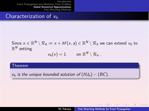
Characterization of vh
Since x ∈ RN \ Rh ⇒ x + hf (x , a) ∈ R
N \ Rh we can extend vh toR
N settingvh(x) = 1 on R
N \ Rh .
Theorem
vh is the unique bounded solution of (HJh) − (BC ).
M. Falcone Fast Marching Methods for Front Propagation
IntroductionFront Propagation and Minimum Time Problem
Global Numerical ApproximationsFast Marching Methods
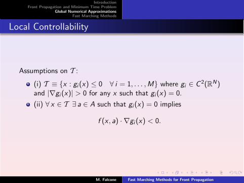
Local Controllability
Assumptions on T :
(i) T ≡ x : gi (x) ≤ 0 ∀ i = 1, . . . ,M where gi ∈ C 2(RN)and |∇gi (x)| > 0 for any x such that gi (x) = 0.
(ii) ∀ x ∈ T ∃ a ∈ A such that gi (x) = 0 implies
f (x , a) · ∇gi (x) < 0.
M. Falcone Fast Marching Methods for Front Propagation
IntroductionFront Propagation and Minimum Time Problem
Global Numerical ApproximationsFast Marching Methods
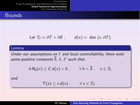
Bounds
Let Tδ ≡ ∂T + δB , d(x) ≡ dist (x , ∂T )
Lemma
Under our assumptions on f and local controllability, there existsome positive constants h, δ, δ′ such that
h Nh(x) ≤ C d(x) + h , ∀ h < h , x ∈ Tδ
andT (x) ≤ c d(x) , ∀ x ∈ Tδ′ .
M. Falcone Fast Marching Methods for Front Propagation
IntroductionFront Propagation and Minimum Time Problem
Global Numerical ApproximationsFast Marching Methods
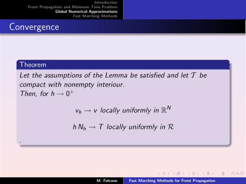
Convergence
Theorem
Let the assumptions of the Lemma be satisfied and let T becompact with nonempty interiour.Then, for h → 0+
vh → v locally uniformly in RN
h Nh → T locally uniformly in R.
M. Falcone Fast Marching Methods for Front Propagation
IntroductionFront Propagation and Minimum Time Problem
Global Numerical ApproximationsFast Marching Methods
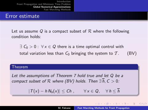
Error estimate
Let us assume Q is a compact subset of R where the followingcondition holds:
∃ C0 > 0 : ∀ x ∈ Q there is a time optimal control with
total variation less than C0 bringing the system to T . (BV)
Theorem
Let the assumptions of Theorem 7 hold true and let Q be acompact subset of R where (BV) holds. Then ∃ h,C > 0:
|T (x) − h Nh(x)| ≤ Ch , ∀ x ∈ Q, ∀ h ≤ h
M. Falcone Fast Marching Methods for Front Propagation
IntroductionFront Propagation and Minimum Time Problem
Global Numerical ApproximationsFast Marching Methods
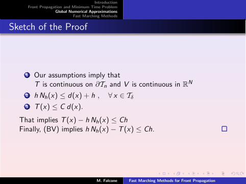
Sketch of the Proof
1 Our assumptions imply thatT is continuous on ∂Tn and V is continuous in R
N
2 h Nh(x) ≤ d(x) + h , ∀ x ∈ Tδ
3 T (x) ≤ C d(x).
That implies T (x) − h Nh(x) ≤ ChFinally, (BV) implies h Nh(x) − T (x) ≤ Ch.
M. Falcone Fast Marching Methods for Front Propagation
IntroductionFront Propagation and Minimum Time Problem
Global Numerical ApproximationsFast Marching Methods
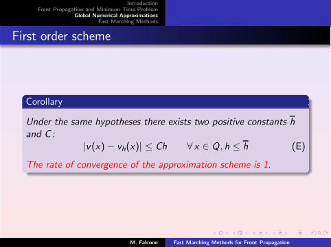
First order scheme
Corollary
Under the same hypotheses there exists two positive constants hand C:
|v(x) − vh(x)| ≤ Ch ∀ x ∈ Q, h ≤ h (E)
The rate of convergence of the approximation scheme is 1.
M. Falcone Fast Marching Methods for Front Propagation
IntroductionFront Propagation and Minimum Time Problem
Global Numerical ApproximationsFast Marching Methods
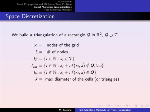
Space Discretization
We build a triangulation of a rectangle Q in R2, Q ⊃ T .
xi = nodes of the grid
L = # of nodes
IT ≡ i ∈ N : xi ∈ T Iout ≡ i ∈ N : xi + hf (xi , a) /∈ Q,∀ aIin ≡ i ∈ N : xi + hf (xi , a) ∈ Qk ≡ max diameter of the cells (or triangles)
M. Falcone Fast Marching Methods for Front Propagation
IntroductionFront Propagation and Minimum Time Problem
Global Numerical ApproximationsFast Marching Methods
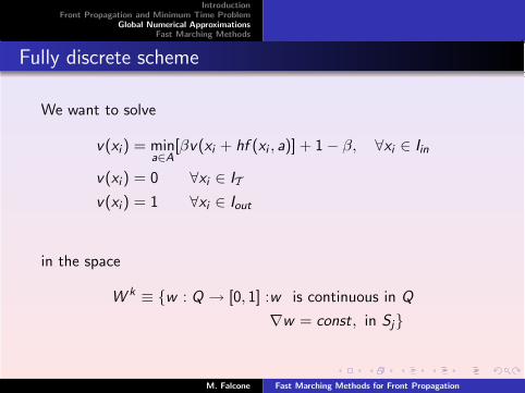
Fully discrete scheme
We want to solve
v(xi) = mina∈A
[βv(xi + hf (xi , a)] + 1 − β, ∀xi ∈ Iin
v(xi) = 0 ∀xi ∈ IT
v(xi) = 1 ∀xi ∈ Iout
in the space
W k ≡ w : Q → [0, 1] :w is continuous in Q
∇w = const, in Sj
M. Falcone Fast Marching Methods for Front Propagation
IntroductionFront Propagation and Minimum Time Problem
Global Numerical ApproximationsFast Marching Methods
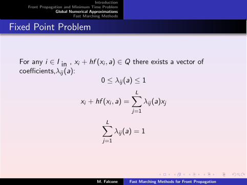
Fixed Point Problem
For any i ∈ I in , xi + hf (xi , a) ∈ Q there exists a vector ofcoefficients,λij (a):
0 ≤ λij(a) ≤ 1
xi + hf (xi , a) =
L∑
j=1
λij(a)xj
L∑
j=1
λij(a) = 1
M. Falcone Fast Marching Methods for Front Propagation
IntroductionFront Propagation and Minimum Time Problem
Global Numerical ApproximationsFast Marching Methods
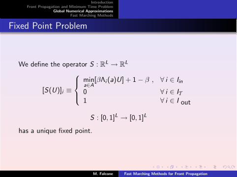
Fixed Point Problem
We define the operator S : RL → R
L
[S(U)]i ≡
mina∈A
[βΛi (a)U] + 1 − β , ∀ i ∈ Iin
0 ∀ i ∈ IT1 ∀ i ∈ I out
S : [0, 1]L → [0, 1]L
has a unique fixed point.
M. Falcone Fast Marching Methods for Front Propagation

IntroductionFront Propagation and Minimum Time Problem
Global Numerical ApproximationsFast Marching Methods
Properties of the scheme S
Theorem
S : [0, 1]L → [0, 1]L and
‖S(U) − S(V )‖∞ ≤ β‖U − V ‖∞
Sketch of the proof . S is monotone, i.e.
U ≤ V ⇒ S(U) ≤ S(V )
Then, for any U ∈ [0, 1]L
1 − β = Si(0) ≤ Si(U) ≤ Si(1) = 1, ∀ i ∈ Iin
where 1 ≡ (1, 1, . . . , 1). This implies, S : [0, 1]L → [0, 1]L
M. Falcone Fast Marching Methods for Front Propagation
IntroductionFront Propagation and Minimum Time Problem
Global Numerical ApproximationsFast Marching Methods
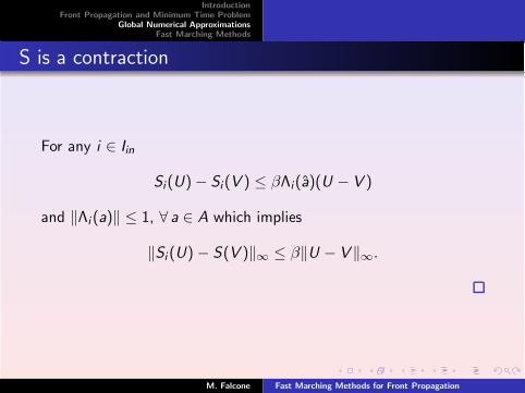
S is a contraction
For any i ∈ Iin
Si(U) − Si(V ) ≤ βΛi(a)(U − V )
and ‖Λi (a)‖ ≤ 1, ∀ a ∈ A which implies
‖Si (U) − S(V )‖∞ ≤ β‖U − V ‖∞.
M. Falcone Fast Marching Methods for Front Propagation
IntroductionFront Propagation and Minimum Time Problem
Global Numerical ApproximationsFast Marching Methods
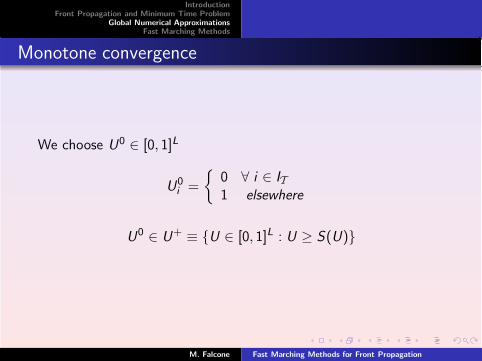
Monotone convergence
We choose U0 ∈ [0, 1]L
U0i =
0 ∀ i ∈ IT1 elsewhere
U0 ∈ U+ ≡ U ∈ [0, 1]L : U ≥ S(U)
M. Falcone Fast Marching Methods for Front Propagation
IntroductionFront Propagation and Minimum Time Problem
Global Numerical ApproximationsFast Marching Methods
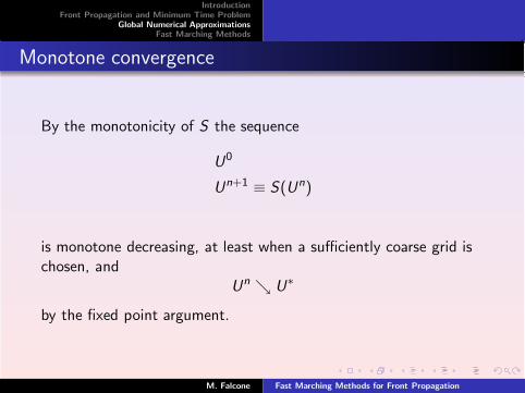
Monotone convergence
By the monotonicity of S the sequence
U0
Un+1 ≡ S(Un)
is monotone decreasing, at least when a sufficiently coarse grid ischosen, and
Un ց U∗
by the fixed point argument.
M. Falcone Fast Marching Methods for Front Propagation
IntroductionFront Propagation and Minimum Time Problem
Global Numerical ApproximationsFast Marching Methods
How the information flows
The information flows from the target to the other nodes of thegrid.In fact, on the nodes in Q \ T , U0
i = 1. But starting from the firststep of the algorithm their value immediately decreases since, bythe local controllability assumption, the Euler scheme drives themto the target.This is the most important fact will allows for a localimplementation of the scheme and to its FM version
M. Falcone Fast Marching Methods for Front Propagation
IntroductionFront Propagation and Minimum Time Problem
Global Numerical ApproximationsFast Marching Methods
A CFL-like condition for FM method
Outline
1 Introduction
2 Front Propagation and Minimum Time Problem
3 Global Numerical Approximations
4 Fast Marching MethodsA CFL-like condition for FM method
M. Falcone Fast Marching Methods for Front Propagation

IntroductionFront Propagation and Minimum Time Problem
Global Numerical ApproximationsFast Marching Methods
A CFL-like condition for FM method
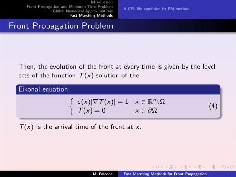
Front Propagation Problem
The main idea of Fast Marching method is based on the frontpropagation point of view. Let ∂Ω be a closed curve (the front) inR
2 and suppose that each of its point moves in the normaldirection with speed c(x).
M. Falcone Fast Marching Methods for Front Propagation
IntroductionFront Propagation and Minimum Time Problem
Global Numerical ApproximationsFast Marching Methods
A CFL-like condition for FM method
Front Propagation Problem
Then, the evolution of the front at every time is given by the levelsets of the function T (x) solution of the
Eikonal equation
c(x)|∇T (x)| = 1 x ∈ Rn\Ω
T (x) = 0 x ∈ ∂Ω(4)
T (x) is the arrival time of the front at x .
M. Falcone Fast Marching Methods for Front Propagation
IntroductionFront Propagation and Minimum Time Problem
Global Numerical ApproximationsFast Marching Methods
A CFL-like condition for FM method
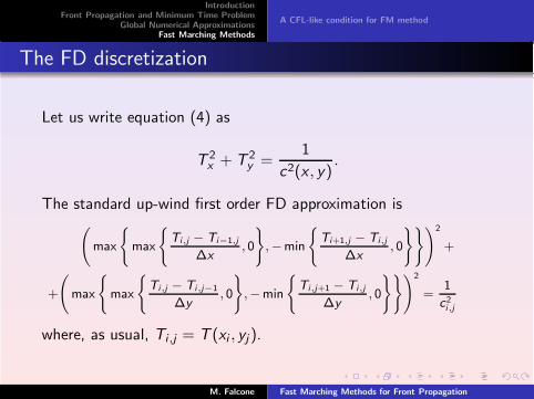
The FD discretization
Let us write equation (4) as
T 2x + T 2
y =1
c2(x , y).
The standard up-wind first order FD approximation is
max
(
max
(
Ti,j − Ti−1,j
∆x, 0
)
,−min
(
Ti+1,j − Ti,j
∆x, 0
))!2
+
+
max
(
max
(
Ti,j − Ti,j−1
∆y, 0
)
,−min
(
Ti,j+1 − Ti,j
∆y, 0
))!2
=1
c2i,j
where, as usual, Ti ,j = T (xi , yj ).
M. Falcone Fast Marching Methods for Front Propagation
IntroductionFront Propagation and Minimum Time Problem
Global Numerical ApproximationsFast Marching Methods
A CFL-like condition for FM method
The Fast Marching method
The FM method was introduced by J. A. Sethian in 1996 [S96]. Itis an acceleration method for the classical iterative FD scheme forthe eikonal equation.
Main Idea (Tsitsiklis (1995), Sethian (1996) )
Processing the nodes in a special ordering one can compute thesolution in just 1 iteration.This special ordering corresponds to the increasing values of T .
The FMM is able to find the ordering corresponding to theincreasing values of (the unknown) T ,while computing. This isdone introducing a NARROW BAND which locates the front.
M. Falcone Fast Marching Methods for Front Propagation
IntroductionFront Propagation and Minimum Time Problem
Global Numerical ApproximationsFast Marching Methods
A CFL-like condition for FM method
The Fast Marching method
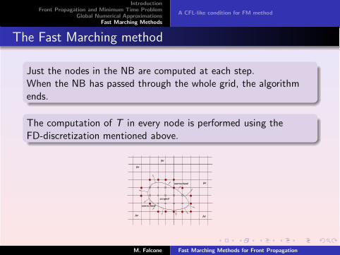
Just the nodes in the NB are computed at each step.When the NB has passed through the whole grid, the algorithmends.
The computation of T in every node is performed using theFD-discretization mentioned above.
far
far
far
far
far
accepted
narrow band
narrow band
M. Falcone Fast Marching Methods for Front Propagation
IntroductionFront Propagation and Minimum Time Problem
Global Numerical ApproximationsFast Marching Methods
A CFL-like condition for FM method
Fast Marching method... marching
In the movie you can see the FM method at work.Once a node is computed, a red spot turns on.
M. Falcone Fast Marching Methods for Front Propagation
IntroductionFront Propagation and Minimum Time Problem
Global Numerical ApproximationsFast Marching Methods
A CFL-like condition for FM method
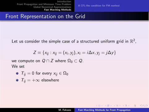
Front Representation on the Grid
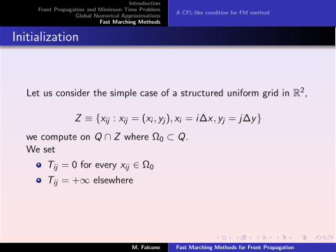
Let us consider the simple case of a structured uniform grid in R2,
Z ≡ xij : xij = (xi , yj), xi = i∆x , yj = j∆ywe compute on Q ∩ Z where Ω0 ⊂ Q.We set
Tij = 0 for every xij ∈ Ω0
Tij = +∞ elsewhere
M. Falcone Fast Marching Methods for Front Propagation
IntroductionFront Propagation and Minimum Time Problem
Global Numerical ApproximationsFast Marching Methods
A CFL-like condition for FM method
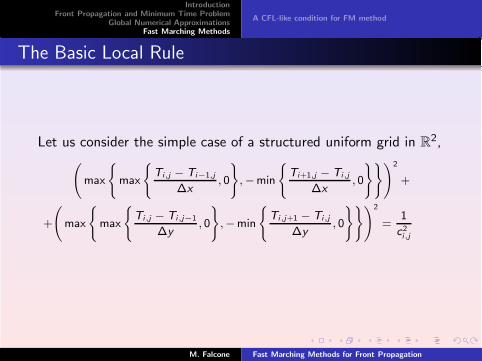
The Basic Local Rule
Let us consider the simple case of a structured uniform grid in R2,
max
(
max
(
Ti,j − Ti−1,j
∆x, 0
)
,−min
(
Ti+1,j − Ti,j
∆x, 0
))!2
+
+
max
(
max
(
Ti,j − Ti,j−1
∆y, 0
)
,−min
(
Ti,j+1 − Ti,j
∆y, 0
))!2
=1
c2i,j
M. Falcone Fast Marching Methods for Front Propagation
IntroductionFront Propagation and Minimum Time Problem
Global Numerical ApproximationsFast Marching Methods
A CFL-like condition for FM method
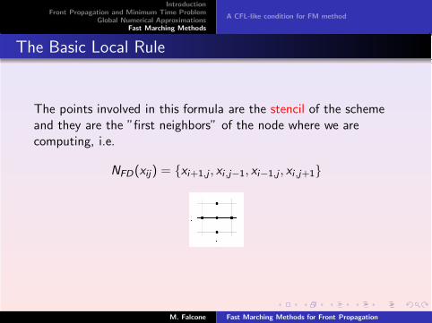
The Basic Local Rule
The points involved in this formula are the stencil of the schemeand they are the ”first neighbors” of the node where we arecomputing, i.e.
NFD(xij) = xi+1,j , xi ,j−1, xi−1,j , xi ,j+1
M. Falcone Fast Marching Methods for Front Propagation

IntroductionFront Propagation and Minimum Time Problem
Global Numerical ApproximationsFast Marching Methods
A CFL-like condition for FM method
Partitioning the nodes
At every iteration (but the last one) we will have three sets ofnodes:
the Accepted nodes, where the values has been alreadycomputed and fixed
the Narrow Band nodes, where the algorithm is computing
the Far nodes, where the algorithm will compute in the nextiterations
We will denote by A(k), NB(k) and F (k) these subsets at the k-thiteration.
Definition
At the iteration k the NB(k) is the set of nodes which are firstneighborsof the nodes in the Accepted region of the previousiteration, i.e. A(k − 1).
M. Falcone Fast Marching Methods for Front Propagation
IntroductionFront Propagation and Minimum Time Problem
Global Numerical ApproximationsFast Marching Methods
A CFL-like condition for FM method
Initialization
Let us consider the simple case of a structured uniform grid in R2,
Z ≡ xij : xij = (xi , yj), xi = i∆x , yj = j∆ywe compute on Q ∩ Z where Ω0 ⊂ Q.We set
Tij = 0 for every xij ∈ Ω0
Tij = +∞ elsewhere
M. Falcone Fast Marching Methods for Front Propagation

IntroductionFront Propagation and Minimum Time Problem
Global Numerical ApproximationsFast Marching Methods
A CFL-like condition for FM method
FMM Algorithm
The algorithm step-by-step, initialization
1 The nodes belonging to the initial front Γ0 are located andlabeled as Accepted. They form the set Γ0. The value of T ofthese nodes is set to 0.
2 NB(1) is defined as the set of the nodes belonging toNFD(Γ0), external to Γ0.
3 Set Ti ,j = +∞ for any (i , j) ∈ NB(1).
4 The remaining nodes are labeled as Far, their value is set toT = +∞.
M. Falcone Fast Marching Methods for Front Propagation
IntroductionFront Propagation and Minimum Time Problem
Global Numerical ApproximationsFast Marching Methods
A CFL-like condition for FM method
FMM Algorithm
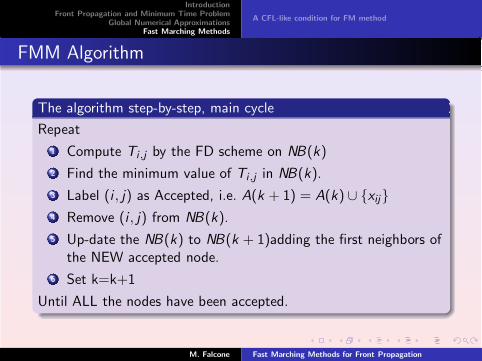
The algorithm step-by-step, main cycle
Repeat
1 Compute Ti ,j by the FD scheme on NB(k)
2 Find the minimum value of Ti ,j in NB(k).
3 Label (i , j) as Accepted, i.e. A(k + 1) = A(k) ∪ xij4 Remove (i , j) from NB(k).
5 Up-date the NB(k) to NB(k + 1)adding the first neighbors ofthe NEW accepted node.
6 Set k=k+1
Until ALL the nodes have been accepted.
M. Falcone Fast Marching Methods for Front Propagation

IntroductionFront Propagation and Minimum Time Problem
Global Numerical ApproximationsFast Marching Methods
A CFL-like condition for FM method
FMM Algorithm
On a finite grid this give the solution after a finite number ofoperations, the solution coincides with the numerical solution ofthe global scheme.
How much it costs ?
We have to compute the solution at every point at most 4 timesand we have to search for the minimum in NB at every iteration.Using a heap-sort method this search costs O(ln(Nnb)). The globalcost is dominated by O(N ln(N)) (N represents the total numberof nodes in the grid).
M. Falcone Fast Marching Methods for Front Propagation
IntroductionFront Propagation and Minimum Time Problem
Global Numerical ApproximationsFast Marching Methods
A CFL-like condition for FM method
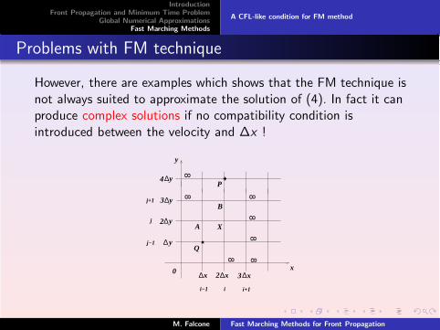
Problems with FM technique
However, there are examples which shows that the FM technique isnot always suited to approximate the solution of (4). In fact it canproduce complex solutions if no compatibility condition isintroduced between the velocity and ∆x !
x
y
0 ∆ ∆2 xx ∆x3
i i+1i−1
∆
∆
∆
∆y
y
y
y
2
3
4
j
j+1
j−1
8 8
Q
A X
B
P8
88
88
M. Falcone Fast Marching Methods for Front Propagation
IntroductionFront Propagation and Minimum Time Problem
Global Numerical ApproximationsFast Marching Methods
A CFL-like condition for FM method
Convergence of FM method
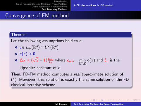
Theorem
Let the following assumptions hold true:
c∈ Lip(Rn) ∩ L∞(Rn)
c(x) > 0
∆x ≤ (√
2 − 1) cmin
Lcwhere cmin= min
Rn\Ωc(x) and Lc is the
Lipschitz constant of c .
Then, FD-FM method computes a real approximate solution of(4). Moreover, this solution is exactly the same solution of the FDclassical iterative scheme.
M. Falcone Fast Marching Methods for Front Propagation
IntroductionFront Propagation and Minimum Time Problem
Global Numerical ApproximationsFast Marching Methods
A CFL-like condition for FM method
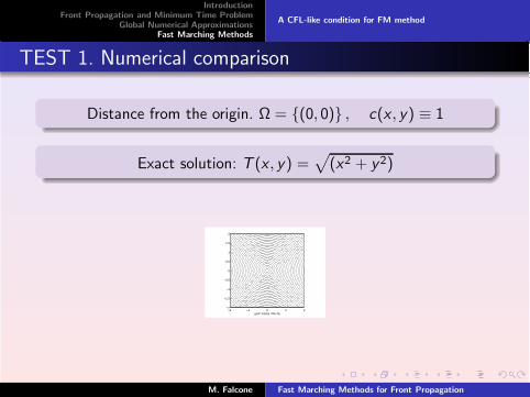
TEST 1. Numerical comparison
Distance from the origin. Ω = (0, 0) , c(x , y) ≡ 1
Exact solution: T (x , y) =√
(x2 + y2)
grid= 51x51 FM−SL−2 −1 0 1 2
−2
−1.5
−1
−0.5
0
0.5
1
1.5
2
M. Falcone Fast Marching Methods for Front Propagation
IntroductionFront Propagation and Minimum Time Problem
Global Numerical ApproximationsFast Marching Methods
A CFL-like condition for FM method
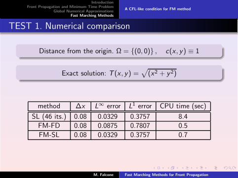
TEST 1. Numerical comparison
Distance from the origin. Ω = (0, 0) , c(x , y) ≡ 1
Exact solution: T (x , y) =√
(x2 + y2)
method ∆x L∞ error L1 error CPU time (sec)
SL (46 its.) 0.08 0.0329 0.3757 8.4
FM-FD 0.08 0.0875 0.7807 0.5
FM-SL 0.08 0.0329 0.3757 0.7
M. Falcone Fast Marching Methods for Front Propagation
IntroductionFront Propagation and Minimum Time Problem
Global Numerical ApproximationsFast Marching Methods
A CFL-like condition for FM method
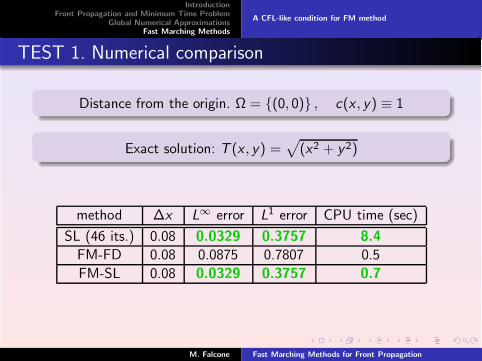
TEST 1. Numerical comparison
Distance from the origin. Ω = (0, 0) , c(x , y) ≡ 1
Exact solution: T (x , y) =√
(x2 + y2)
method ∆x L∞ error L1 error CPU time (sec)
SL (46 its.) 0.08 0.0329 0.3757 8.4
FM-FD 0.08 0.0875 0.7807 0.5
FM-SL 0.08 0.0329 0.3757 0.7
M. Falcone Fast Marching Methods for Front Propagation
IntroductionFront Propagation and Minimum Time Problem
Global Numerical ApproximationsFast Marching Methods
A CFL-like condition for FM method
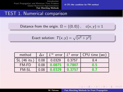
TEST 1. Numerical comparison
Distance from the origin. Ω = (0, 0) , c(x , y) ≡ 1
Exact solution: T (x , y) =√
(x2 + y2)
method ∆x L∞ error L1 error CPU time (sec)
SL (46 its.) 0.08 0.0329 0.3757 8.4
FM-FD 0.08 0.0875 0.7807 0.5
FM-SL 0.08 0.0329 0.3757 0.7
M. Falcone Fast Marching Methods for Front Propagation
IntroductionFront Propagation and Minimum Time Problem
Global Numerical ApproximationsFast Marching Methods
A CFL-like condition for FM method
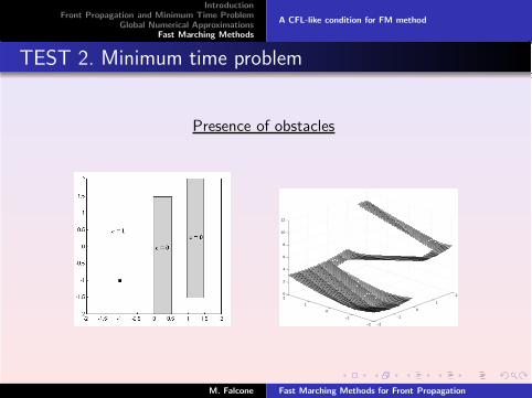
TEST 2. Minimum time problem
Presence of obstacles
−2
−1
0
1
2
−2
−1
0
1
20
2
4
6
8
10
12
M. Falcone Fast Marching Methods for Front Propagation
IntroductionFront Propagation and Minimum Time Problem
Global Numerical ApproximationsFast Marching Methods
A CFL-like condition for FM method
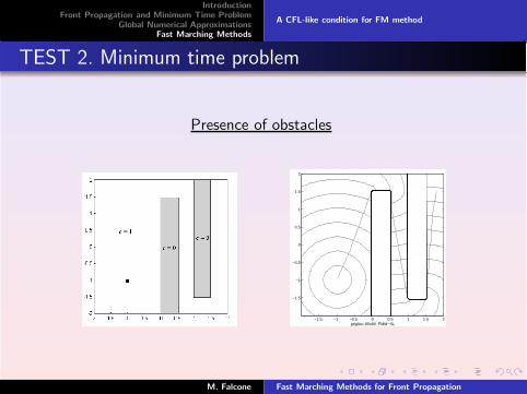
TEST 2. Minimum time problem
Presence of obstacles
−1.5 −1 −0.5 0 0.5 1 1.5 2
−1.5
−1
−0.5
0
0.5
1
1.5
2
griglia= 80x80 FMM−SL
M. Falcone Fast Marching Methods for Front Propagation
IntroductionFront Propagation and Minimum Time Problem
Global Numerical ApproximationsFast Marching Methods
A CFL-like condition for FM method
Some references
[1 ] E. Cristiani, M. Falcone, Fast semi-Lagrangian schemes for the Eikonal equation and applications, SIAM J.Numer. Anal. (2007), .
[2 ] J. A. Sethian, A fast marching level set method for monotonically advancing fronts, Proc. Natl. Acad. Sci.USA, 93 (1996), 1591-1595.
[3 ] J.A. Sethian, Fast Marching Methods, SIAM Review, No.2 41, 199–235 (1999)
[4 ] J. A. Sethian, Level Set Methods and Fast Marching Methods: Evolving Interfaces in Computational
Geometry, Fluid Mechanics, Computer Vision and Materials Science, Cambridge University Press, 1999.
[5 ] J. A. Sethian, A. Vladimirsky, Ordered upwind methods for static Hamilton-Jacobi equations: theory and
algorithms, SIAM J. Numer. Anal., 41 (2003), pp. 325–363.
[6 ] J. N. Tsitsiklis, Efficient algorithms for globally optimal trajectories, IEEE Tran. Automatic. Control, 40(1995), 1528-1538.
[7 ] A. Vladimirsky, Static PDEs for time-dependent control problems, Interfaces and Free Boundaries 8/3(2006), 281-300.
M. Falcone Fast Marching Methods for Front Propagation

IntroductionFront Propagation and Minimum Time Problem
Global Numerical ApproximationsFast Marching Methods
A CFL-like condition for FM method
Coming soon
Sweeping
Group Marching
Extensions to more general problems and equations
The case when c(x , t) can change sign (Lecture 3)
M. Falcone Fast Marching Methods for Front Propagation