FAST INVERSION OF THE RADON TRANSFORM USING - …fa/preprints/logpolFBP.pdf · Fast Inversion of...

FAST INVERSION OF THE RADON TRANSFORM USINGLOG-POLAR COORDINATES AND PARTIAL BACK-PROJECTIONS∗

FREDRIK ANDERSSON†

Abstract. In this paper a novel filtered back-projection algorithm for inversion of a discretizedRadon transform is presented. It makes use of invariance properties possessed by both the Radontransform its dual. By switching to log-polar coordinates, both operators can be expressed in adisplacement invariant manner. Explicit expressions for the corresponding transfer functions arecalculated. Furthermore, by dividing the back-projection into several partial back-projections, it canbe performed by means of finite convolutions, and hence implemented by an FFT-algorithm. In thisway, a fast and accurate reconstruction method is obtained.

Key words. Radon transform, filtered back-projection.

AMS subject classifications. 44A12, 64R10, 92C55

1. Introduction. The two-dimensional Radon transform is the mapping from(sufficiently regular) functions on R2 to line integrals in R2,

Rf(θ, s) =∫

x·θ=s

f(x) dx, (1.1)

i.e. the integral of f over the line with normal direction θ and (signed) distances to the origin. The standard method of inverting the Radon transform, filteredback-projection, uses the back-projecting operator R#, which integrates over all linespassing through a point. The main drawback of computer implementations of thismethod is that they are relatively computationally expensive. The computationalcomplexity in computing the back-projection is of type O(q3). Over the years, sev-eral faster (O(q2 log q)) reconstruction methods have been developed, but the ones offiltered back-projection type are mostly preferred in applications for reasons of qual-ity. In this paper we make use of invariance properties of R#, for reconstruction inO(q2 log q) time.

It is immediate to see that the Radon transform is invariant under rotation. Inaddition it has the scale invariantly property, for c > 0,

R[f(c ·)](θ, s) = cR[f(·)](θ, cs).

The back-projecting operator is also invariant under rotation and in fact strictly scaleinvariant. By changing to log-polar coordinates (θ, s) 7→ (θ, ρ), where s = eρ, itis possible to express both the Radon transform (apart from scaling) and the back-projecting operator by means of convolutions. This opens for the construction of anFFT-based algorithm for fast computation of the back-projection.

However, the nonlinear coordinate change s 7→ eρ makes direct usage of theconvolution structure impractical in computing the total back-projection. A uniformlysampled interval in the ρ-variable containing points close to the origin in the s-variable,must be very densely sampled in order to obtain a descent sample distance with respectto s, for points not close to the origin. However, this problem can be avoided throughusing the concept of partial back-projection introduced in §3.3.

∗Submitted October 7, 2003.†Centre for Mathematical Sciences, Lund University/LTH, P.O. Box 118, S-22100 Lund, Sweden.

([email protected]).

1

2 Fredrik Andersson

Making use of the above invariance properties by introducing log-polar coordi-nates, in combination with the concept of partial back-projection, thus allows devel-opment of a fast algorithm for computing the back-projection. The quality of thereconstructions made from the algorithm presented in this paper is about be thesame as the one calculated in the standard setting, but in addition the method iscomparable with other fast ones in speed.

2. Preliminaries. When defined on the unit cylinder S = S1 × R, the two-dimensional Radon transform (defined by (1.1)) is even, i.e. Rf(−θ,−s) = Rf(θ, s),since each line can be parameterized in two ways. Here S1 denotes the unit circle,parameterized by [−π, π). Sometimes it is convenient to work on S+ = S1 × R+ orS1/2 = [−π/2, π/2)×R instead, both sufficient to describe all lines in the plane. It iswell known that the Radon transform as a mapping S(R2) → S(S) is invertible. In thispaper we are especially interested in dealing with the Radon transform of compactlysupported functions, and inversion techniques for such. The Radon transform can then(possibly combined with a suitable preceding translation) be viewed as a invertiblemapping C∞0 (S+) → C∞0 (S+).

The dual Radon transform R# integrates functions defined on S over subsets ofS corresponding to lines passing through a point x ∈ R2,

R#g(x) =∫

S1g(θ, x · θ) dθ. (2.1)

It is dual in the sense that∫

S(Rf)(θ, s)g(θ, s) dsdθ =

∫

R2f(x)(R#g)(x) dx,

and is commonly in the literature referred to as the back-projecting operator.In order to write the inversion formula for the Radon transform in a simple form,

one introduces the operator J acting on (sufficiently regular) functions in S, definedby

J =∂

∂sH,

where H denotes the Hilbert transform with respect to the second variable in S, i.e.

Hf(x) =1π

∫

R

1x− y

f(y) dy,

where the integral is interpreted as a principal value.An inversion formula then reads as

f =12

1√2πR#JRf. (2.2)

For more details, c.f. [14]. The factor 1/2 on the right hand side is due to the factthat in the interpretation of R#, each line is taken into account twice. Using insteadS+ or S1/2, the factor 1/2 is removed. The operator J is cannot be defined directlyon S+, hence it is instead defined as the restriction of the action on S to S+.

In practice, where Radon data are given on a discrete sampling grid, the op-erator J is usually implemented by a discrete convolution in the s-variable with abandlimited filter. More specifically, one makes use of the formula

W ∗ f = R#(w1∗ Rf), (2.3)

Fast Inversion of the Radon Transform using Log-polar Coordinates 3

where1∗ denotes one dimensional convolution with respect to the second variable,

s, in S, and where W and w are related by W = R#w, c.f. [14]. By choosingW approximating a δ-distribution, we obtain an approximate reconstruction. Morespecifically, one usually chooses W = Wb to be radially symmetric and band-limitedwith some cut-off frequency b. When chosen in this way, w = wb depends only on thes-variable, in which it is band-limited by b, c.f. [14].

By approximating the continuous convolution in 2.3 by a discrete one, the filteringstep w

1∗Rf can be accomplished, by use of FFT, with a time complexity O(q2 log q),if the number of parallel lines and directions both are q. A more time-consumingstep is the computation of the back-projection. The straightforward numerical im-plementation of R# uses, for each discrete direction sample point θj , some kind ofinterpolation in the s-variable to approximate g(θj , x · θj) in (2.1), in combinationwith some quadrature rule on S1:

R#d g(x) =

∑

j

αjg(θj , x · θj).

Here, roughly q values are summed up at each reconstruction point, giving a timecomplexity of orderO(q3) for q2 reconstruction points. Reconstruction methods whichare based on (2.2) are referred to as filtered back-projection algorithms.

Several suggestions on how to invert the Radon transform in O(q2 log q) time hasappeared in the literature during the years. Most common are Fourier based methods,making use of the ”Fourier slice theorem”:

Fs(Rf)(θ, σ) = F2(f)(σθ),

where Fs denotes the one-dimensional Fourier transform with respect to s on S,and F2 denotes the two-dimensional cartesian Fourier transform on R2. Using thiswith natural uniform discretizations of the θ- and σ-variables results in knowledgeof the two-dimensional Fourier transform on the right hand side on a non-uniformgrid. Direct interpolation onto a rectangular grid followed by FFT inversion resultin O(q2 log q) complexity, but gives rise to unacceptable artifacts. To cope with thisone can e.g. use over-sampling combined with more sophisticated interpolation, assuggested in [14], or use fast Fourier algorithms for unequally spaced data, c.f. [2],[16].

Fast techniques for filtered back-projection algorithms are presented in [15], [5],[3], [4], where the back-projection is calculated recursively in O(q2 log q) time.

In this paper we present a back-projection algorithm which uses a log-polar gridfor treating the back-projection part. Log-polar grids have previously been used in anART fashion, cf [8], to derive a system of linear equations, which after regularizationcan be treated with standard numerical techniques. However, according to [8], thisapproach was not successful in competition with the standard filtered back-projectionalgorithm, neither in speed nor quality.

To begin with we give a discussion about some properties of the continuous Radontransformation and its dual, which are both of interest on its own, and useful for thediscrete approximative inversion presented below. A somewhat reminiscent discussionis given in [1], where some closed form formulas, involving Tchebychev polynomials,are given starting from a polar representation. A numerical implementation is alsopresented, in [1], but the number of computations needed are of order O(q3).

4 Fredrik Andersson

3. Properties of the continuous Radon transform and its dual.

3.1. Convolution operators. Consider the cylinder S+ = S1×R+ as a group,provided with the algebraic structure inherited from its components, i.e. the additivegroup S1 = R/2πZ (addition modulo 2π), and the multiplicative group R+ (positivereal numbers).

Let z = (θ, s) ∈ S+. The group operation on S+, written multiplicatively, is

(θ1, s1)(θ2, s2) = ((θ1 + θ2) mod 2π, s1s2) .

The Haar measure on S+ = S1 × R+ is inherited from the components, and canbe written dh(z) = dθ ds/s. Hence

∫

S+f(z) dh(z) =

∫ 2π

0

∫ ∞

0

f(θ, s) dθds

sfor f ∈ C∞0 (S+) ,

where C∞0 (S+) is the C∞0 class on S+, with support outside the origin S1 × 0. TheHaar property means that

∫

S+f(wz) dh(z) =

∫

S+f(z) dh(z) for w ∈ S+ , f ∈ C∞0 (S+) .

There exists a natural isomorphism between S+ and the punctured complex planeC = C \ 0 considered multiplicatively, parameterized by (θ, s) ←→ seiθ. Using thecartesian representation z = x + iy for C, the Haar measure on S+ can be written

dh(z) = dθds

s=

dx dy

x2 + y2.

If C is represented instead by coordinates

seiθ = eρeiθ, ρ ∈ R, (3.1)

which we will refer to as log-polar coordinates, then the Haar measure on S+ becomes

dh(z) = dθ dρ.

Let λ be the distribution that represents integration over the line x = 1 in C,

λ : f 7−→∫ ∞

−∞f(1, y) dy =

∫

Cf(x, y)δ(x− 1) dx dy , f ∈ S(S+) .

In the (θ, s) = z representation, it can be written

λ : f 7−→∫ π

2

−π2

f(θ,1

cos θ)

1cos2 θ

dθ =∫

S+f(θ, s)δ(s cos θ − 1)s ds dθ =

=∫

S+f(z)λ(z) dh(z) , with λ(z) = s2δ(s cos θ − 1) .

Let lines in C be denoted Lξ, where ξ is the footprint of the normal of the linethrough the origin. The Radon transform (1.1) can be expressed as

g(ξ) = Rf(ξ) = |ξ|∫

S+f(zξ)λ(z) dh(z) . (3.2)


This follows from the fact that in the last integral, the distribution λ is applied toa function that is obtained from f by a similarity transformation of the coordinateplane, such that the line Lξ is transferred to L1, which is the support of λ. Using |ξ|to compensate for the change in scale, we obtain the Radon transform.

The duality between points on a line in C and lines through a point in C motivatesinterest for the distribution

λ# : f 7−→∫ π

2

−π2

f(θ, cos θ) dθ =∫ π

2

−π2

∫

R+

f(θ, s)δ(cos θ − s) ds dθ =

=∫

S+f(z)λ#(z) dh(z) , with λ#(z) = sδ(cos θ − s) .

which, if f is interpreted as a function on lines in C, is the integral over all linesthrough the point 1 ∈ C. Also note that

∫ β

α

∫

R+

f(s, θ)λ#(s, θ) ds dθ (3.3)

is the integral over all lines through the point 1 ∈ C with normal direction in theinterval [α, β].

The distributions ζ(z) = λ(1/z) and ζ#(z) = λ#(1/z), formally defined by

ζ : f 7−→∫

S+f(1/z)λ(z) dh(z),

ζ# : f 7−→∫

S+f(1/z)λ#(z) dh(z) , f ∈ C∞0 (S+) .

will be crucial in what follows. In the (θ, s) = z representation, these can explicitlybe written

ζ(z) = s−2δ(s−1 cos θ − 1),ζ#(z) = δ(s cos θ − 1).

Using the Haar property on the integral, the formula (3.2) can also be written

Zf(ξ) =Rf(ξ)|ξ| =

∫f(z)ζ(

ξ

z) dh(z) . (3.4)

Apart from the scaling factor |ξ|, the Radon transform thus can be expressed as aconvolution on C∞0 (S+).

For the back-projecting operator (2.1), note that if ξ ∈ C and if g ∈ C∞0 (S+) isinterpreted as a function on lines in C, then

R#g(ξ) =∫

S+g(ξz)λ#(z) dh(z),

is the integration over all lines that passes through ξ. Hence, by using the Haarproperty again,

R#g(ξ) =∫

S+g(z)ζ#(

ξ

z) dh(z), (3.5)

6 Fredrik Andersson

or in the log-polar representation

R#g(ρ, θ) =∫

S+g(ρ′, θ′)ζ#(ρ− ρ′, θ − θ′) dρ dθ. (3.6)

This fact opens a possibility to perform the inversion in (2.2) by means of an appro-priate Fourier transform.

3.2. Fourier analysis. The Fourier transform FS+ = F on S+ is a compoundof the Fourier series transform on S1 and the Mellin transform on R+:

F : f(θ, s) 7−→ g(µ, σ) =∫ 2π

0

∫ ∞

0

e−iµθs−σf(θ, r)ds

sdθ, µ ∈ Z , σ ∈ C .

In log-polar representation (3.1) the Fourier transform instead becomes a compoundof the Fourier series transform and the Laplace transform on R,

F : f(θ, ρ) 7−→ g(µ, σ) =∫ 2π

0

∫ ∞

−∞e−iµθe−σρf(θ, r) dρ dθ, µ ∈ Z , σ ∈ C .

As the operators Z in (3.5) and R# can be expressed as convolutions on S+, itsuffices to calculate the corresponding transfer functions for determination of Fζ andFζ#.

It is readily verified using (3.2) that for ξ = reiψ,

Zf(ξ) =∫

S+f(θ + ψ, rs)δ(s cos θ − 1)s ds dθ =

∫ π/2

−π/2

f(θ + ψ,r

cos θ)

1cos2 θ

dθ.

Let f(θ, s) = sσeiµθ. Then the transfer function for Z is obtained by

Zf(ξ) =∫ π/2

−π/2

eiµ(θ+ψ)( r

cos θ

)σ 1cos2 θ

dθ = rσeiµψ

∫ π/2

−π/2

eiµθ(cos θ

)−σ−2dθ =

= f(ξ)Fζ(µ, σ).

Here, Fζ(µ, σ) converges in the classical sense for Re σ < −1, where it defines ananalytic function.

Similarly, the transfer function for the back-projecting operator R# is obtainedby

R#f(ξ) =∫ π/2

−π/2

eiµθ(r cos(θ − ψ))σ dθ =∫ π/2

−π/2

eiµ(θ+ψ)(r cos θ)σ dθ =

= rσeiµψ

∫ π/2

−π/2

eiµθ(cos θ)σ dθ = f(ξ)Fζ#(µ, σ),

and Fζ#(µ, σ) converges in the classical sense for Re σ > −1.Note that Fζ(µ, σ) and Fζ#(µ, σ) are not simultaneously (classically) well de-

fined, and furthermore the resemblance between the two Fourier transforms:

Fζ(µ, σ) = Fζ#(µ,−σ − 2).

In order to derive explicit expressions for the Fourier transforms above, we provethe following proposition:


Proposition 3.1. Let µ ∈ Z, α > −1, and

P (µ, α) =∫ π

2

−π2

eiµθ cosα(θ) dθ. (3.7)

Then P (µ, α) is an analytic function given by

P (µ, α) =Γ(α+1

2 )Γ(α+22 )Γ( 1

2 )Γ(α+µ

2 + 1)Γ(α−µ2 + 1)

.

Proof. By two partial integrations it follows that

−µ2P (µ, α) =∫ π/2

−π/2

d2

dθ2(eiµθ)(cos θ)α

dθ =

=∫ π/2

−π/2

eiµθ(α(α− 1)(cos θ)α−2 − α2(cos θ)α) dθ =

= α(α− 1)P (µ, α− 2)− α2P (µ, α),

giving rise to the following recursion formula:

P (µ, α− 2) =α

α− 1(1− µ2

α2)P (µ, α).

Hence, for all positive integers n,

P (µ, α− 2) =( n∏

k=0

α + 2k

α + 2k − 1

)( n∏

k=0

(1− µ2

(α + 2k)2))P (µ, α + n) =

=2nΓ(α

2 + n + 1)Γ(α

2 )Γ(α−1

2 + n)2nΓ(α+1

2 + n)

( n∏

k=0

(1− µ2

(α + 2k)2))P (µ, α + 2n) =

=B(α

2 − 12 , 1

2 )B(n + α

2 + 12 , 1

2 )

( n∏

k=0

(1− µ2

(α + 2k)2))P (µ, α + 2n), (3.8)

where B denotes the beta function and where the identity

B(m,n) =Γ(m)Γ(n)

Γ(m + n + 1),

has been used. Recall that the beta function is defined by

B(m + 1, n + 1) = 2∫ π/2

0

(cos θ)2m+1(sin θ)2n+1 dθ. (3.9)

Introduce

hn(t) =(cos t)n

B(n2 + 1

2 , 12 )

,

which by using 3.9 easily is shown to satisfy,

limn→∞

hn(t) = δ(t),

8 Fredrik Andersson

for |t| < π. Using this in combination with (3.7), we rewrite (3.8),

P ( µ , α− 2) =

= limn→∞

B(α

2− 1

2,12)( n∏

k=0

(1− µ2

(α + 2k)2)) ∫ π/2

−π/2

eiµθ (cos θ)α+2n

B(n + α2 + 1

2 , 12 )

dθ =

= B(α

2− 1

2,12)( ∞∏

k=0

(1− µ2

(α + 2k)2)). (3.10)

From the identity

Γ2(n + 1)Γ(n + ix + 1)Γ(n− ix + 1)

=∞∏

k=1

(1 +x2

(n + k)2),

on page 699 in [20], cf. formula (64), it follows that

P (µ, α) = B(α + 1

2,12)( ∞∏

k=1

(1− µ2

(α− 2k)2))

=Γ(α+1

2 )Γ(α+22 )Γ( 1

2 )Γ(α+µ

2 + 1)Γ(α−µ2 + 1)

.

By extending P (µ, α) of proposition 3.1 analytically, we conclude that

Fζ(µ, σ) =Γ(−σ−1

2 )Γ(−σ2 )Γ( 1

2 )Γ(−σ+µ

2 )Γ(−σ−µ2 )

,

Fζ#(µ, σ) =Γ(σ+1

2 )Γ(σ+22 )Γ( 1

2 )Γ(σ+µ

2 + 1)Γ(σ−µ2 + 1)

. (3.11)

Below, figure 3.1 illustrates properties of the function Fζ#(µ, iw). Its energy content

Fig. 3.1. The absolute value and real part of Fζ#(µ, iω)

is mainly contained in a neighborhood of the origin and along the line µ = 0. Notethat although its absolute value it rather smooth, the real and imaginary parts arestrongly oscillating.


3.3. Partial back-projection. Our aim is to present a fast procedure for com-puting the back-projection as a discrete convolution on a uniformly sampled grid inlog-polar coordinates. However, the counterpart in polar coordinates will be non-uniform, corresponding to a dense assembling of grid points close to the origin in C.This assembling causes large variation in the density of both reconstruction grid pointsand data sample points. By moving the origin it is possible to obtain a more uniformstructure within the grid points of the reconstruction region, but this does not simplifythe treatment of the data sample points. The difficulty here is the need of dealingwith lines with various distance to the origin, and this problem consist independentlyof where the origin is situated, if lines with all directions must be considered.

To cope with this, we divide the measurement data into m ≥ 3 (disjoint) sets,each containing lines with directions in an interval of length π

m . Corresponding toeach such set, we choose an origin outside the region of interest, in such a way thatthe back-projection from lines with directions within each interval, cf. (3.3), can becalculated by means of finite integrals. We refer to this procedure as partial back-projection. By putting these partial back-projections together it is possible to obtaina total back-projection. To begin with, we consider one special case.

Let β = πm for some positive integer m ≥ 3, and let aR denote the radius of the

largest circle inscribed in a sector with unit radius and central angle β, cf. figure

β

am

aR

β/2

β/2

O

Lθ,s

Fig. 3.2. Lines with directions θ ∈ [−β2, β

2], passing through a circle inscribed in a segment

(3.2). It is straightforward to show that

aR =sin(β

2 )

1 + sin(β2 )

. (3.12)

Consider the set of all lines, Lθ,s with normal directions |θ| ≤ β2 , with respect to the

symmetry axis of the sector, passing through the inscribed circle, c.f. figure 3.2. It isclear that the normal distances to the origin, s, of these lines will be in the interval(am, 1), where

am + aR = (1− aR) cos(β

2), (3.13)

or by using 3.12

am =cos(β

2 )− sin(β2 )

1 + sin(β2 )

. (3.14)

10 Fredrik Andersson

Suppose that f ∈ C∞0 has its support inside the inscribed circle, and that Rf(θ, s) isknown. Let

h0(θ, s) = χβJRf(θ, s),

where χβ is the characteristic function of the set

θ : −β

2≤ θ <

β

2.

The contribution

f0(x) =∫ β

2

− β2

JRf(θ, θ · x) dθ

from the back-projection of lines with directions in the interval (−β2 , β

2 ) in log-polarcoordinates, for x inside the inscribed circle, may by use of (3.6) and (3.3) be writtenas

f0(θ, ρ) =∫ β

2

− β2

∫ 0

ln(am)

h0(θ′, ρ′)ζ#(θ − θ′, ρ− ρ′) dρ′dθ′.

Furthermore, if ζ#p (θ, ρ) is defined as the periodic extension of ζ#(θ, ρ) for θ ∈ [β, β]

and ρ ∈ [ln(am), 0], then

f0(θ, ρ) =∫ β

−β

∫ 0

ln(am)

h0(θ′, ρ′)ζ#p (θ − θ′, ρ− ρ′) dρ′dθ′, (3.15)

when θ ∈ [−β2 , β

2 ] and ρ ∈ [1− 2aR, 1]. This is due to the fact that the integral lengthin the θ′-direction is twice the θ′-support of h0(θ′, ρ′), and to the fact that the valuesof h0(θ′, ρ′) for ρ′ outside [ln(am), 0], is of no importance in (partial) back-projectingfor x = (θ, ρ) inside the inscribed circle. Thus, replacing h0(θ′, ρ′) with a periodicalextension of h0(θ′, ρ′) as above, which is equivalent to extending ζ#, does not influencethe result. Hence, the partial back-projection at points of interest can be calculatedas a periodic convolution.

Now, let f ∈ C∞0 (Ω2), where Ω2 denotes the unit disc in R2, and suppose thatRf(θ, s) is known. By dividing the data into m different parts, each spanning anangle interval of β, and to each such set make a suitable change of coordinates, onetransforms the full back-projection problem to m subproblems of the form above. Anillustration of the procedure, for m = 3, is given in figure 3.3. The coordinate transfor-mation x → xν , consists of, after a rescaling with aR, a rotation by β degrees followeda translation of the origin O to Oν . Each part is then of the form discussed above, andadding the respective partial back-projections gives the total back-projection, sinceeach partial back-projection integrates over disjunct intervals (−β/2 + νβ, β/2 + νβ),which together covers an interval length of mβ = π. For the sake of completeness, weinclude the details.

Let ν = 0, . . . ,m− 1, and introduce for each ν new coordinates

xν = aR

(cos(νβ) sin(νβ)− sin(νβ) cos(νβ)

)x +

(1− aR

0

),


O O0

O1

O2

Fig. 3.3. Reconstruction from three views

and let fν(xν) = f(x). Each fν then has its support inside a circle inscribed in asector with unit radius and central angle β, as in figure 3.2. Let

hν = χβJRfν .

The following relation, easily verified,

xν · θ = x · aR(θ + νβ) + (1− aR) cos(θ), (3.16)

will be useful. Any line in the x-coordinate system may be written

Lθ+νβ,s = x|x · (θ + νβ) = s,for some ν ∈ 0, . . . , m − 1 and −β

2 ≤ θ < β2 . In the xν-coordinate system the

corresponding line may then, by using (3.16), be written

Lνθ,aRs+(1−aR) cos(θ) = xν |xν · θ = aRs + (1− aR) cos(θ).

Hence,

hν(θ, s) = χβJRf(θ + νβ,s− (1− aR) cos(θ)

aR) (3.17)

The total back-projection for some point x inside the support of f can now, again byusing (3.16), be written as

R#JRf(x) =∫

S1JRf(θ, x · θ) dθ =

= 2m−1∑ν=0

∫ β2

− β2

JRf(θ + νβ, (θ + νβ) · x) dθ =

= 2m−1∑ν=0

∫ β2

− β2

hν(θ, aR(θ + νβ) · x + (1− aR) cos(θ)) dθ =

= 2m−1∑ν=0

∫ β2

− β2

hν(θ, xν · θ) dθ,


where the factor 2 in the last expressions is due to the fact that the total integrationis only performed on half of S1.

We now have reduced the full back-projection problem to making m partial re-constructions of the form discussed above. For future references, let us introduce

fνr (xν) =

1√2π

∫ β2

− β2

hν(θ, xν · θ) dθ. (3.18)

The inversion formula (2.2) then allows us to write

f(x) =m−1∑ν=0

fνr (xν). (3.19)

We’ve deduced that it is possible to compute the total back-projection as a sumof partial back-projection. The sharp cutoff caused by χβ will however in practicegive rise to artifacts in form of sharp lines with normal directions corresponding tothe cutoff angles. Therefore it is desirable to make a smoother cutoff. This requirethat the supports in θ-direction for the respective hν overlap. The angle β is then notequal to π

m , where m is the number of partial back-projections to be used, but larger.Suppose π

m ≤ β ≤ 2πm . By letting

η(t) =

e

−β2

β2−4t2 , if |t| < β2 ;

0, otherwise,

a smooth cutoff function

χβ,m(θ) =η(θ)

η(θ) + η( πm − arccos(cos θ)))

(3.20)

with support in [−β2 , β

2 ], can be formed. Since

∞∑

k=−∞χβ,m(θ + k

π

m) ≡ 1,

it follows that the reconstruction (3.19) is still valid if χβ in (3.17) is replaced byχβ,m.

4. Discrete log-polar reconstruction.

4.1. Principles. In this section we present a description on how to use themethod of section 3.3 for making reconstructions from discrete measurements. Forsimplicity we deal with the case of parallel beam data. Hopefully, other types of datawill be treated in a sequel to this paper. Let f ∈ C∞0 (Ω2), let g = Rf be sampled at(θj , sl), j = 0, . . . , p − 1, l = −q, . . . , q (parallel beam geometry), where θj ∈ S1 and

sl = lq , and let h = wb

1∗g, in accordance to (2.3). The latter quantity is approximatedby the discrete convolution

wbd∗ g(θj , s) =

1q

q∑

l=−q

wb(s− sl)g(θj , sl). (4.1)


What now remains for reconstruction is the back-projection. To this end, let theinteger m be the number of partial reconstruction to be used, let β = π/mβ , supposethat m and mβ divides p, and let θj = −β

2 + jπp .

For the construction of the discrete back-projecting operator we will make use ofthe interpolation results discussed in §A. To begin with, suppose h(θ, s) is known,and sample hν defined in (3.17),with χβ replaced by χβ,m from (3.20), uniformly in alog-polar representation (θj , ρi) covering (−β

2 , β2 )× (− ln(am), 0). Let I∆2 = I(∆θ,∆ρ)

be a direct quasi-interpolator of order o2, with kernel ϕ(θ, ρ) = ϕθ(θ)ϕρ(ρ), where ∆θand ∆ρ is the grid spacing of (θj , ρi).

Construct

hν∗(θ, ρ) =

∑

j

∑

i

hν [j, i]ϕ(θ − θj

∆θ,ρ− ρi

∆ρ),

as an approximation of hν . Now the back-projection of hν∗ , for xν represented by

θ ∈ [−β2 , β

2 ] and ρ ∈ [1− 2aR, 1], can be written

R#hν∗(θ, ρ) =

∫ β

−β

∫ 0

ln(am)

hν∗(θ − θ′, ρ− ρ′)ζ#(θ′, ρ′) dρ′ dθ′ =

∫ β

−β

∫ 0

ln(am)

(∑

j

∑

i

hν [j, i]ϕ(θ − θ′ − θj

∆θ,ρ− ρ′ − ρi

∆ρ))ζ#(θ′, ρ′) dρ′ dθ′ =

∑

j

∑

i

hν [j, i]Z(θ − θj , ρ− ρi), (4.2)

where

Z(θ, ρ) =∫ β

−β

∫ 0

ln(am)

ϕ(θ − θ′

∆θ,ρ− ρ′

∆ρ)ζ#(θ′, ρ′) dθ′dρ′. (4.3)

This follows by exchanging the order between sums and integrals. Note that Z isindependent of the Radon data.

Due to this structure, it is particularly convenient to make reconstructions onsome uniformly sampled (θ, ρ)-grid, e.g. the same upon which hν was resampled, asthis enables computation of the discrete convolutions by means of two-dimensionalFFT (after appropriate zero padding). Once the partial back-projections fν

r are com-puted on the (θj , ρi)-grid, it remains only to interpolate them onto a cartesian rep-resentation and add the results to obtain a reconstruction f . A survey of relevantinterpolation methods is given in §A

The procedure discussed above involves three quasi-interpolators. The first one,which was not discussed above, is needed in the resampling onto the uniform (θj , ρi)-grid. Let it be denoted by I∆1 = I 1

q+1/2, and its interpolating order by a1. Hence,

h[j, i] above should be replaced by (I∆1h)[j, i]. The second one, represented by I∆2

above, is naturally incorporated into Z(θ, ρ) as described by 4.3, and the third one,I∆3 of interpolating order o3, is needed when adding up the parts. In short, a pseudocode for the reconstruction is presented below:

Algorithm 4.1.function f=iradonlp(g,m,mbeta);

[p,q]=size(g);h=wfilter(g);


FZ=fft2(get_Z(p,q,mbeta));chi=get_chi(m,mbeta,q);f=0;for nu=0:m-1,

hlp=interp_pol2lp(chi.*h(nu*p/m+(0:p/mbeta-1),:));hlp=[hlp;zeros(size(hlp))];flp=ifft2(FZ*fft2(hlp));f=f+interp_lp2cart(flp);

end;end;

Let us discuss the first interpolation step slightly more into detail. Since, foreach fixed θ, h(θ, s) is band-limited by b, the first interpolation step can actually becomputed exactly from h(θj , sl) by (A.1), as long as the Nyquist condition b < πq issatisfied. However, this is quite time consuming, and ruins the time gain achieved byusing log-polar coordinates in the back-projection.

The non-uniformity between data in polar and log-polar representation respec-tively, requires use of more sample points in the log-polar representation in orderto avoid too much loss of information. Suppose ∆ρ = − ln(am)

q′−1 and ρi = 1 − i∆ρ,i = 0, . . . , q′ − 1, where q′ = κ(2q + 1) for some over sample factor κ. If the filterband-width of (4.1) is given by b = πq, then by choosing

κ > − ln(am)2aR

the knowledge of h(θ, ρi) at all grid points suffice to reconstruct h(θ, ρi), cf. [21]. Atypical choice here is κ = 2.

Remark. The combination of uniformly spaced FFT and the interpolation schemedescribed above is in principle the same as in the procedures used in fast Fouriertransforms for unequally spaced data, cf. [2]. Usage of the fast implementationsavailable for such routines allows simple and fast implementation of the algorithmdescribed above. It should be stressed that although the tools used are the same asin e.g. [16], the underlying method is quite different; the one of this paper is basedon the filtered back-projection technique, whereas the others has been based on theFourier slice theorem.

4.2. Error analysis. In the algorithm described above, errors are introducedat several places. The first one is made in the filtering step, caused by the discreteconvolution (4.1). This is common for algorithms of filtered back-projection type, andestimated in [14] by

|wbd∗ g − wb ∗ g|(θ, s) ≤ 1

2

∫

σ≥b

|σ|n−1f(σθ) dσ = e1. (4.4)

To describe the ones caused by interpolation we need to introduce modified Sobolevnorms, for polar and log-polar coordinates, respectively. The main reason for notusing the natural definitions is that since each filtering h of Radon data of somecompactly supported function is not compactly supported, and especially since thefiltering does not vanish in a neighborhood of s = 0, the natural Sobolev norm inlog-polar coordinates of h is in general, if it exists, infinite.

Similarly to the definition (A.6), let

||f ||Hγpol

=∑

|α|≤γ

∫ ∫|Dα

θ,sf(θ, s)|2χpol(θ, ρ) dθ ds,


and

||f ||Hγlp

=∑

|α|≤γ

∫ ∫|Dα

θ,ρf(θ, ρ)|2χlp(θ, ρ) dθ dρ,

be polar and log-polar Sobolev norms, respectively. Here f(θ, s) and f(θ, ρ) are con-nected through the change of variables

ρ = ln(s− (1− aR) cos(θ)

aR), (4.5)

χpol is a smooth cutoff function equal to one on (−β2 , β

2 )× (−1, 1), and similarly χlp

equal to one on (−β2 , β

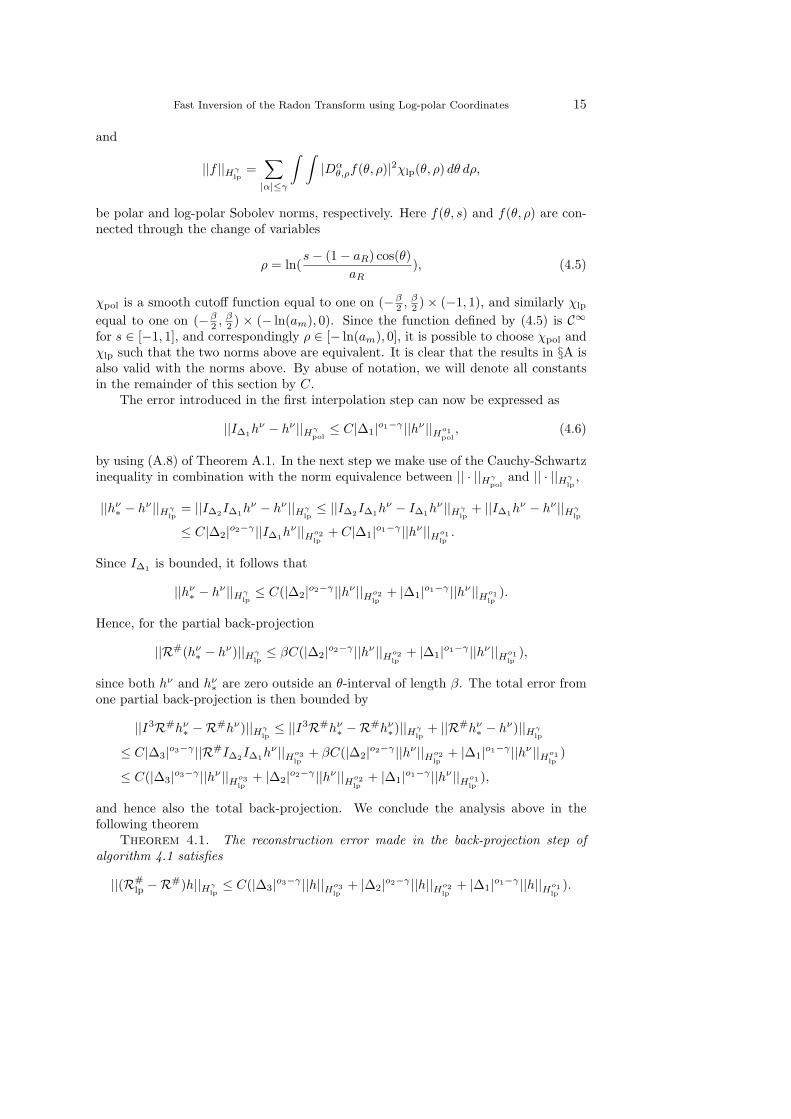
2 ) × (− ln(am), 0). Since the function defined by (4.5) is C∞for s ∈ [−1, 1], and correspondingly ρ ∈ [− ln(am), 0], it is possible to choose χpol andχlp such that the two norms above are equivalent. It is clear that the results in §A isalso valid with the norms above. By abuse of notation, we will denote all constantsin the remainder of this section by C.

The error introduced in the first interpolation step can now be expressed as

||I∆1hν − hν ||Hγ

pol≤ C|∆1|o1−γ ||hν ||Ho1

pol, (4.6)

by using (A.8) of Theorem A.1. In the next step we make use of the Cauchy-Schwartzinequality in combination with the norm equivalence between || · ||Hγ

poland || · ||Hγ

lp,

||hν∗ − hν ||Hγ

lp= ||I∆2I∆1h

ν − hν ||Hγlp≤ ||I∆2I∆1h

ν − I∆1hν ||Hγ

lp+ ||I∆1h

ν − hν ||Hγlp

≤ C|∆2|o2−γ ||I∆1hν ||Ho2

lp+ C|∆1|o1−γ ||hν ||Ho1

lp.

Since I∆1 is bounded, it follows that

||hν∗ − hν ||Hγ

lp≤ C(|∆2|o2−γ ||hν ||Ho2

lp+ |∆1|o1−γ ||hν ||Ho1

lp).

Hence, for the partial back-projection

||R#(hν∗ − hν)||Hγ

lp≤ βC(|∆2|o2−γ ||hν ||Ho2

lp+ |∆1|o1−γ ||hν ||Ho1

lp),

since both hν and hν∗ are zero outside an θ-interval of length β. The total error from

one partial back-projection is then bounded by

||I3R#hν∗ −R#hν)||Hγ

lp≤ ||I3R#hν

∗ −R#hν∗)||Hγ

lp+ ||R#hν

∗ − hν)||Hγlp

≤ C|∆3|o3−γ ||R#I∆2I∆1hν ||Ho3

lp+ βC(|∆2|o2−γ ||hν ||Ho2

lp+ |∆1|o1−γ ||hν ||Ho1

lp)

≤ C(|∆3|o3−γ ||hν ||Ho3lp

+ |∆2|o2−γ ||hν ||Ho2lp

+ |∆1|o1−γ ||hν ||Ho1lp

),

and hence also the total back-projection. We conclude the analysis above in thefollowing theorem

Theorem 4.1. The reconstruction error made in the back-projection step ofalgorithm 4.1 satisfies

||(R#lp −R#)h||Hγ

lp≤ C(|∆3|o3−γ ||h||Ho3

lp+ |∆2|o2−γ ||h||Ho2

lp+ |∆1|o1−γ ||h||Ho1

lp).


We end up by a quantitative remark on the estimates above. The frequencycontent of (direct) quasi-interpolators is, generally speaking, one at a neighborhoodof zero and dies out for higher frequencies, cf. proposition A.3. In principle theymimic sinc-interpolation, where the frequency content of the kernel is a box functioncentered at the origin. Thus, the error introduced by replacing the operator R# withI∆3R#I∆2 is mainly due to what happens with Radon data far away from the origin.Now, consider the back-projection kernel of figure 3.1. Apart from along the lineµ = 0, most of its energy lies in a neighborhood of the origin. As pointed out above,if data (limited to s ∈ [ln(am), 1]) is smooth with respect to polar coordinates, it issmooth also in the log-polar representation. The fact that data is band-limited withrespect to s in combination with the fast decay in the ω-direction should thereforekeep the errors relatively small in practise.

4.3. Time complexity and implementation. Let us analyze algorithm 4.1slightly more in detail. The first filtering step is the same as in other filtered back-projection algorithms, and can be implemented by p FFT operations of length 4q intime O(pq log(q)). At the first interpolation step, each interpolation (I∆1h

ν)(θj , ρi)consists of a weighted sum of h(θj , sl) at points with sl within a kernel length distanceto ρi. Hence this step is O(d1pq′) = O(2d1pκq), with d1 the kernel length of I∆1 .Similarly, each interpolation from log-polar coordinates to cartesian ones is made bya weighted sum, in both θ and ρ-directions, giving a time complexity of O(4d3q

2),where d3 is the kernel area of I∆3 , if reconstruction is made on a (2q + 1)× (2q + 1)-grid. Assuming both d1 and d3 to be relatively small, and using the optimal relationbetween p and q in parallel beam geometry, p = πq, cf. [14], we arrive at a timecomplexity of O(q2) for both interpolation steps.

Note that for both the interpolation weights above as well for the computation ofthe kernel Z defined in (4.3), only geometry matters, i.e. these can be pre-computed tosave time. What remains are then the two-dimensional FFT steps. Taken into accountthe needed zero-padding, 2m two-dimensional FFT operations of size ( 2p

m × q′) arerequired. This is performed in time O(pq log(pq)) = O(q2 log(q)), i.e. at the samecomplexity as other fast reconstruction methods. However, in comparison with e.g.Fourier slice-reconstruction on a (2q+1)× (2q+1) grid, the preceding constant of theleading term is worse. In principle this is due to over-sampling factors of κ and 2 inthe s and θ directions, respectively, and that both transformation and inversion areused. Together, this cause a worsening of a factor of about ten. However, that is incomparison with the most simplest Fourier slice-reconstruction, with its well knownsevere drawbacks in quality, and without effort of speeding up our proposed method(it is possible to use the zero-padded structure to decrease needed calculations). Itshould be added that that more sophisticated slice-reconstruction schemes also requireover-sampling for adequate results.

Throughout §4.1 we worked with direct quasi-interpolators. The structure ofalgorithm 4.1 easily incorporates usage of the pre-filtering required by e.g. splineinterpolators discussed in §A. Required pre-filtering for I∆1 can thus be included inwb of (4.1), and pre-filtering needed for I∆2 and I∆3 can be included in Z definedby (4.3). This allows usage of spline interpolators without increasing computationalcost, and thus allows higher interpolation order than the ones achieved by directinterpolators of the same kernel length.

4.4. Simulations. Finally, let us look at some numerical results. In these sim-ulations we have used cubic spline interpolators for I∆1 , I∆2 and I∆3 , m = 4 partialreconstructions, mβ = 3, and κ = 2. The number of parallels and directions are


Fig. 4.1. Impulse responses for log-polar (above) versus classical back-projection (below) atpoints (0.1233, 0.3816), (0.0998, 0.0998), (0.8004,−0.0020) and (−0.3229,−0.2368) respectively fromleft to right.

q = 512 and p = 768 respectively. Furthermore, to limit the regularization impactfrom the choice of filter in the filtering step, the Ram-Lak -filter suggested by Ra-machandran and Lakshminarayanan in [17] is used.

In e.g. [10], analytic expression for the Radon transform of functions being char-acteristic function of ellipses are derived. We use such functions as reconstructionsobjects, since they allow us to sample the Radon data exactly.

In the section we study two types of reconstruction. First we use characteristicfunction of small circles as approximations of delta functions, and then the Shepp-Logan phantom, described in [10], an artificial slice of a head built up by characteristicfunctions of ellipses.

Below are shown impulse responses at four different points for log-polar and clas-sically computed back-projection, respectively. The reconstructions show quite highresemblance. Reconstruction on a cartesian grid makes the impulse response varyslightly depending on the placement of the impulse. It is worth noting that the re-sponses usually are wider and smoother, when the ordinary filters of the filtering stepare used.

Next we turn our attention to the Shepp-Logan phantom, cf. figure 4.2. Thetrue head phantom carries an intensity of 1.02 at its inner, a border of intensity 2.0,”eyes” at 1.0 and additional ellipses at 1.03 (except at intersections). The two topimages of figure 4.2 show reconstruction by log-polar (right) and traditional (left)back-projection. These seem almost identical, and it is hard to draw further conclu-sions. For a better perspective, we have chosen to plot the two reconstructions along ahorizontal line through the ”mouth” part of the head, at the center of figure 4.2. More


50 100 150 200 250 300 350 400 450 500

50

100

150

200

250

300

350

400

450

5001

1.005

1.01

1.015

1.02

1.025

1.03

1.035

1.04

50 100 150 200 250 300 350 400 450 500

50

100

150

200

250

300

350

400

450

5001

1.005

1.01

1.015

1.02

1.025

1.03

1.035

1.04

−0.5 −0.4 −0.3 −0.2 −0.1 0 0.1 0.2 0.3 0.4 0.51.015

1.02

1.025

1.03

50 100 150 200 250 300 350 400 450 500

50

100

150

200

250

300

350

400

450

500 −0.15

−0.1

−0.05

0

0.05

0.1

0.15

50 100 150 200 250 300 350 400 450 500

50

100

150

200

250

300

350

400

450

500−1

−0.8

−0.6

−0.4

−0.2

0

0.2

0.4

0.6

0.8

1x 10

−3

Fig. 4.2. Upper left shows reconstruction using log-polar coordinates, upper right classicalreconstruction. At center a comparison between the two along a horizontal line. The two lowerimages show the difference between the two reconstruction at different scales.

precisely the values of the two reconstructions along row 410 has been plotted, withan offset of -0.001, to discriminate them. The two reconstructions display almost thesame appearance, except minor disparities at the points of discontinuity. For furthercomparison, differences between the two reconstructions are shown in figure 4.2 below,with different intensity scales. The left one display differences in the reconstructionof the high intensity border around the skull. At right we can also see differences atthe other discontinuity parts, but note the low intensity span. This image also clearlyshows a slightly inhomogeneous assembling of lines outside the head, an affect of thedifferent techniques used.

5. Conclusion. In this paper we have made use of the invariance propertiesof the Radon transform and its dual to construct a method of inversion based ona log-polar representation. An analysis of the continuous case has been presentedas well as analytical expressions for the kernels. To deal with the non-uniformityof the discrete case, the concept of partial reconstructions was introduced. The non-uniformity also enforces the discrete reconstruction developed to rely on interpolation.


Fortunately, these can be invoked in the reconstruction procedure, for constructionof a fast and accurate back-projection algorithm, based on use of the (uniform) two-dimensional FFT. The algorithm presented has a time complexity of O(q2 log(q)), thesame as other fast reconstruction algorithms. From the tests presented in this paper,its accuracy seems to be practically the same as the one traditional back-projectionalgorithms have.

Appendix. Some properties of convolution interpolators. To obtain theerror estimates needed above, some results on classical interpolation and samplingtheory are needed. Since the focus of this article lies on practical tomography recon-struction, we’ll settle with qualitative results.

According to Whittaker-Shannon’s sampling theorem, for any b-band-limited func-tion f , i.e. a function with a Fourier transform f(ξ) vanishing for |ξ| > b, it is possibleto reconstruct f given the uniformly sampled values of f at xk = kT , where T = π/b.The reconstruction formula reads as

f(x) =∑

k∈Zf(xk)sinc(x− xk). (A.1)

A drawback of this sinc-based interpolation is the slow decay of the sinc-function.The sinc-interpolation above is an example of convolution-based interpolation foruniformly sampled data:

IT f(x) =∑

j∈Zcj [f ]ϕ(

x

T− j); (A.2)

a mixed convolution of a set of coefficients and an interpolation kernel ϕ. The coeffi-cients cj [f ] are generally obtained from

cTj [f ] = µ(f(

·T

+ j)), (A.3)

where µ is a linear functional. For an overview of convolution-based interpolation, c.f.[13]. The operator IT is said to be an interpolator (sometimes referred to as cardinalinterpolator) if IT f coincides with f at the sample points.

In some cases it is of more interest if IT manages to reconstruct polynomials of acertain order correctly. To this end, IT is said to be an quasi-interpolator of order p+1if it successfully interpolates all polynomials of degree p. The special simple case whereci[f ] = f(xi) is important, referred to as direct quasi-interpolators. A commonly usedinterpolator is the Key’s short cubic interpolator [11], with interpolation kernel

ϕ(x) =

(a + 2)|x|3 − (a + 3)|x|2 + 1, 0 ≤ |x| < 1;a(|x|3 − 5|x|2 + 8|x| − 4), 1 ≤ |x| < 2;0, otherwise,

(A.4)

parameterized by a. Since ϕ(x) is zero at a cardinal points it follows that Keys’s shortcubic interpolator really is an interpolator.

The most widely used indirect interpolators are the spline interpolators, [18]. TheB-spline kernel of order m is defined by

ϕBm = (12χ[− 1

2 , 12 ] +

12χ(− 1

2 , 12 )) ∗ · · · ∗ (

12χ[− 1

2 , 12 ] +

12χ(− 1

2 , 12 )) (m + 1 factors). (A.5)

It is readily verified that ϕBm consists of piecewise polynomials of degree m, and thatit is supported in (−m+1

2 , m+12 ).


Regarding the error of convolution-based interpolation, the Strang-Fix conditionsplays an important role. The error estimates are carried out in a Sobolev frame work,where Hγ(Rn) or Hγ of real order γ consists of the functions f such that

||f ||2Hγ =∑

|α|≤γ

||Dαf ||2L2(Rn), is finite, (A.6)

where

Dαf = (∂

∂x1)α1 . . . (

∂

∂xn)αn , α = (α1, . . . , αn).

For the restriction of Hγ0 to compactly supported functions, Hγ

0 is used as notation.The following theorem can be found in [19]

Theorem A.1. (Strang-Fix theorem)Let p be a positive integer and suppose ϕ ∈ Hp

0 . Then the following conditions areequivalent:

1. ϕ(0) 6= 0, but ϕ has zeros of order at least p + 1 at the other points of 2πZn:

Dαϕ(2πj) = 0 if 0 6= j ∈ Zn, |α| ≤ p. (A.7)

2. for |α| ≤ p,∑

j∈Zn

jαϕ(x− j)

is a polynomial in x1, . . . , xn with leading term ϕ(0)tα.3. For each f ∈ Hp+1 there are coefficients cT

j such that as |T | → 0,

||f −∑

j∈Zn

cTj ϕ(

·T− j)||Hs ≤ Cs|T |p+1−s||f ||Hp+1 , 0 ≤ s ≤ p, (A.8)

where Cs is independent of f . Furthermore, these coefficients are bounded by∑

j∈Zn

|cTj [f ]|2 ≤ K||f ||2H0 , (A.9)

where K is independent of f .Above, it is required that the kernel ϕ has compact support, a requirement that

can replaced by a decay condition, c.f. [7]. These conditions indicate that given somekernel ϕ satisfying (A.7) of order p+1, it is possible to construct a (quasi)-interpolatorsatisfying (A.8), i.e. approximating of order p + 1. Under the right assumptions, thisis true, but not a direct consequence of theorem A.1.

The characterization of the conditions needed on the functional µ in (A.3) is outof the scope of this paper, c.f. [6]. For our purposes it suffices be able to deal withdirect quasi-interpolators. The following theorem is a simplified version of theorem4.1 in [9]:

Theorem A.2. Let IT be a direct quasi-interpolator of order p+1, equipped withkernel ϕ with sufficient decay, and let f ∈ Hp+1. Then

||f − IT f ||H0 ≤ C|T |p+1||f ||Hp+1 . (A.10)


The following proposition for direct quasi-interpolators is easily shown by use ofPoisson’s summation formula:

Proposition A.3. Let IT f(x) =∑

j f(jT )ϕ( xT − j). Then IT is a quasi-

interpolator of order p + 1 if and only if

ϕ(2πj) = δ[j], j ∈ Zn

Dαϕ(2πj) = 0, j ∈ Zn and |α| ≤ p.(A.11)

where δ[j] denotes the (discrete) Kronecker delta function.Note that condition (A.7) differs slightly from A.11, since (A.7) imposes no

requirements on the derivatives of ϕ at the origin. It is straightforward to showthat Key’s short cubic interpolator satisfies the Strang-Fix conditions up to quasi-interpolating order 3, if the free parameter is chosen as a = 1

2 .For R1, the simplest interpolation kernel which satisfies (A.7) is the B-spline

kernel, since

ˆϕBm(ξ) = (sin(ξ/2)

ξ/2)m+1.

Thus, every ϕ which satisfies (A.7) is a multiple of ˆϕBm , ϕ = ˆϕBmE, where E is asuitable entire function, and hence every other interpolation kernel can be obtainedas a convolution of a B-spline kernel.

However, it is not possible to construct a direct quasi-interpolator with ϕBm asinterpolation kernel for m > 2. This is due to the fact that the Taylor expansion ofϕBm is

ˆϕBm(ξ) = 1− (1 + m)ξ2

24+O(ξ4), (A.12)

which contradicts (A.11).The natural question of how the mapping cj [f ] (i.e. the functional µ) should

be chosen for obtaining good (quasi)-interpolators now arises. The approach givenhere is based on the one outlined in [12]. From (A.2) follows that (in R) for thecorresponding IT to be an interpolator,

f(xk) =∑

j∈ZcTj [f ]ϕ(

x

T− j) =

∑

j∈ZcTj [f ]ϕ(k − j), (A.13)

must be satisfied. This (infinite) system of equations may be solved by means of theZ-transform, for which (A.13) becomes

(∑

j∈Zϕ(j)Zj)C(Z) = F (Z).

Looking for the impulse response, i.e. the response of f [k] = δ[k], we obtain

Cδ(Z) =1∑

j∈Z ϕ(j)Zj. (A.14)

This can be used to construct a direct interpolator. Note that if IT is a directinterpolator, then the function reconstructed from the sequence

f [k] = δ[k]


is the interpolation kernel. Using this yields

ψ(x) =∑

j∈Zc1j [δ]ϕ(x− j) =

∑

j∈Zc1j [δ](δj ∗ ϕ)(x),

where δk(x) = δ(x− k) denotes the translated Dirac distribution. Hence,

ψ(ξ) = (∑

j∈Zc1j [δ]e

−ijξ)ϕ(ξ) = Cδ(e−iξ)ϕ(ξ). (A.15)

For the sake of concreteness we consider the cubic spline interpolator, with interpo-lation kernel

ϕB3(x) =

(3|x|3 − 6|x|2 + 4)/6, |x| ≤ 1;(2− |x|)3/6, 1 ≤ |x| ≤ 2;0, otherwise,

explicitly calculated from (A.5). For this choice, the rightmost quantity of (A.13)becomes

f(xk) =16cTk−1[f ] +

46cTk [f ] +

16cTk+1[f ].

Equation (A.14) then becomes

Cδ(Z) =6

Z + 4 + Z−1, (A.16)

giving the impulse response

cj [δ] = (−1)k(2−√3)|j|c0[δ], c0[δ] = 43√

3. (A.17)

Since 0 < 2−√3 < 1, the sequence ck[δ] oscillates and decays exponentially.Combining (A.15) and (A.16) yields the direct interpolation kernel

ˆψB3(ξ) =6

4 + 2 cos(ξ)(sin ξ/2

ξ/2)4.

Hence, from the Taylor expansion

ˆψB3(ξ) = 1− 1720

ξ4 +O(ξ6),

it follows from the requirement stated in (A.11) that the cubic spline interpolatorconstructed above is a quasi-interpolator of order 4. The advantage of such an in-terpolator, in contrast to e.g. the sinc interpolator of (A.1), is that due to the smallsupport of the B-spline kernels, it is possible to perform the interpolation by using asmall number of evaluations once the coefficients cj has been calculated.

In this paper, two dimensional interpolators are also needed. Whenever so, tensorproducts of one dimensional interpolators, i.e.

IT f(x) =∑

j∈Zn

cTj [f ]ϕ1(

x1

T1− j1) · · ·ϕn(

xn

Tn− jn),

are used. In such cases |T | = max(T1, T2) in theorems A.1 and A.2.


REFERENCES

[1] S. Alliney, Digital reconstruction of images from their projections on polar coordinates, SignalProcessing, 3 (1981), pp. 135–145.

[2] G. Beylkin, On the fast Fourier transform of functions with singularities, Appl. Comput.Harmon. Anal., 2 (1995), pp. 363–381.

[3] M. L. Brady, A fast discrete approximation algorithm for the Radon transform, SIAM J.Comput., 27 (1998), pp. 107–119 (electronic).

[4] A. Brandt, J. Mann, M. Brodski, and M. Galun, A fast and accurate multilevel inversionof the Radon transform, SIAM J. Appl. Math., 60 (2000), pp. 437–462 (electronic).

[5] P. Danielsson and M. Ingerhed, Backprojection in O(N2 log N) time, IEEE Nucl. Sci. Symp.,2 (1997), pp. 1279–1283.

[6] C. de Boor, Quasiinterpolants and approximation power of multivariate splines, in Compu-tation of curves and surfaces (Puerto de la Cruz, 1989), vol. 307 of NATO Adv. Sci. Inst.Ser. C Math. Phys. Sci., Kluwer Acad. Publ., Dordrecht, 1990, pp. 313–345.

[7] C. de Boor and R.-Q. Jia, Controlled approximation and a characterization of the localapproximation order, Proc. Amer. Math. Soc., 95 (1985), pp. 547–553.

[8] P. P. B. Eggermont, Tomographic reconstruction on a logarithmic polar grid, IEEE Trans.Med. Imag., MI-2 (1983), pp. 40–48.

[9] R. Q. Jia and J. Lei, Approximation by multi-integer translates of functions having globalsupport, J. Approx. Theory, 72 (1993), pp. 2–23.

[10] A. C. Kak and M. Slaney, Principles of computerized tomographic imaging, IEEE Press,New York, 1988.

[11] R. G. Keys, Cubic convolution interpolation for digital image processing, IEEE Trans. Acoust.,Speech, Sig. Proc., 29 (1981), pp. 1153–1160.

[12] E. Maeland, On the comparison of interpolation methods, IEEE Trans. Med. Imag., 7 (1988),pp. 213–217.

[13] Meijering, A cronology of interpolation. from ancient astronomy to modern signal and imageprocessing, Proceedings of the IEEE, 90 (2002), pp. 319–342.

[14] F. Natterer, The mathematics of computerized tomography, B. G. Teubner, Stuttgart, 1986.[15] S. Nilsson, Applications of Fast Backprojection Techniques for Some Inverse Problems Integral

Geometry, PhD thesis, Linkoping University, Sweden, 1997.[16] D. Potts and G. Steidl, A new linogram algorithm for computerized tomography, IMA J.

Numer. Anal., 21 (2001), pp. 769–782.[17] G. N. Ramachandran and A. V. Lakshminarayanan, Three-dimensional reconstruction from

radiographs and electron micrograhs: application of convolutions instead of fourier trans-forms, Proceedings of Natural Academic Sciences. US, 68 (1971).

[18] I. J. Schoenberg, Contributions to the problem of approximation of equidistant data by ana-lytic functions. Part A and B.

[19] G. Strang and G. Fix, A fourier analysis of the finite element variational method, Construc-tive Aspects of Functional Analysis, G. Geymonat, ed., C.I.M.E., (1973), pp. 793–840.

[20] E. W. Weisstein, CRC concise encyclopedia of mathematics, Chapman & Hall/CRC, BocaRaton, FL, second ed., 2003.

[21] A. I. Zayed, Advances in Shannon’s sampling theory, CRC Press, Boca Raton, FL, 1993.

FAST INVERSION OF THE RADON TRANSFORM USING - …fa/preprints/logpolFBP.pdf · Fast Inversion of...

Documents

Transcript of FAST INVERSION OF THE RADON TRANSFORM USING - …fa/preprints/logpolFBP.pdf · Fast Inversion of...