Fast Guided Global Interpolation for Depth and...

Fast Guided Global Interpolationfor Depth and Motion

Yu Li1, Dongbo Min2, Minh N. Do3, and Jiangbo Lu1 ?

1 Advanced Digital Sciences Center, Singapore2 Chungnam National University, Korea

3 University of Illinois at Urbana-Champaign, US

Abstract. We study the problems of upsampling a low-resolution depthmap and interpolating an initial set of sparse motion matches, with theguidance from a corresponding high-resolution color image. The com-mon objective for both tasks is to densify a set of sparse data points,either regularly distributed or scattered, to a full image grid througha 2D guided interpolation process. We propose a unified approach thatcasts the fundamental guided interpolation problem into a hierarchical,global optimization framework. Built on a weighted least squares (WLS)formulation with its recent fast solver – fast global smoothing (FGS)technique, our method progressively densifies the input data set by ef-ficiently performing the cascaded, global interpolation (or smoothing)with alternating guidances. Our cascaded scheme effectively addressesthe potential structure inconsistency between the sparse input data andthe guidance image, while preserving depth or motion boundaries. Toprevent new data points of low confidence from contaminating the nextinterpolation process, we also prudently evaluate the consensus of the in-terpolated intermediate data. Experiments show that our general inter-polation approach successfully tackles several notorious challenges. Ourmethod achieves quantitatively competitive results on various benchmarkevaluations, while running much faster than other competing methodsdesigned specifically for either depth upsampling or motion interpolation.

Keywords: Image-guided interpolation, depth upsampling, optical flow

1 Introduction

Dense depth or optical flow maps often serve as a fundamental building blockfor many computer vision and computational photography applications, e.g., 3Dscene reconstruction, object tracking, video editing, to name a few. An activerange sensing technology such as time-of-flight (ToF) cameras has been recentlyadvanced, emerging as an alternative to obtaining a depth map. It provides 2Ddepth maps at a video rate, but the quality of ToF depth maps is not as good asthat of a high-quality color camera. The depth map is of low-resolution and noisy,

? This study is supported by the HCCS grant at the ADSC from Singapore’s Agencyfor Science, Technology and Research (A*STAR). Corresponding author: J. Lu

2 Yu Li, Dongbo Min, Minh N. Do, Jiangbo Lu

Noisy low res. ToF depth High res. color guidance FGI (ours)

Color frame and sparse matches [39] Epic‐LA [35]

Motion interpolation

Depth upsampling68× 86 1088 × 1376

GF [21] AR [43]

FGI (ours)

Fig. 1. Using the same guided interpolation pipeline, our technique gives strong resultsfor two tasks: (top) depth upsampling and (bottom) optical flow field interpolation.Local or non-local methods (e.g. GF [21] and Epic-LA [35]) are usually efficient, butsuffer from limitations like copying texture from the color guidance (green arrows) andinability to interpolate pixels in a distance (green rectangle). Methods using compli-cated models and global optimization (e.g. AR [43]) can obtain high quality results,but are often rather slow in computation. Our method, with a unified framework forboth problems, is 1000× faster than AR [43] and even faster than local methods, whileyielding competitive results when compared with state-of-the-art task-specific methods.

and thus a post-processing for depth upsampling is usually required to enhancethe quality of depth maps. Over the years, numerous approaches for optical flowestimation have also been developed, but several challenging issues still remain,including large displacements, non-rigid fine motion, large occlusion, and flowboundaries. To address these issues, modern optical flow approaches often use adiscriminative descriptor (or patch) matching to estimate sparse or quasi-densemotion matches. These important anchor points are used to interpolate a denseflow map, which is then embedded into subsequent optimization procedures.

One prevailing strategy for both depth upsampling and motion field interpo-lation is via a guided interpolation that uses an associated high-quality color im-age, exploiting the correlation between the color guidance and the depth/motiondata. For depth upsampling, many methods based on the guided interpolationhave been proposed with either local or global formulations [21, 43, 10, 12, 17, 22,28–30, 34, 32]. Similarly, the guided motion field interpolation has been activelyadopted as a key element in state-of-the-art optical flow approaches [35, 6, 39, 14,26, 25, 8]. Though both tasks share the same goal of densifying a set of sparse in-put data points to a full image grid, most existing interpolation approaches havebeen developed in isolation, tailored to either the depth upsampling or motiondensification tasks due to different characteristics of two data sets. For instance,ToF depth observations are noisy but regularly distributed in the high-resolutionimage grid, while sparse motion matches after outlier removal are typically reli-able but highly scattered with a varying density of valid motion data across animage. In addition, existing interpolation methods are usually complicated andcomputationally inefficient.

Fast Guided Global Interpolation for Depth and Motion 3

We propose a unified approach to cast the fundamental guided interpolation(or densification) problem for both depth and motion data into a hierarchi-cal, global optimization framework. Leveraging a recent fast global smoothing(FGS) technique [31] based on a weighted least squares (WLS) formulation [16],our method progressively densifies the input data set by efficiently performinga cascaded, guided global interpolation (or smoothing). While most existing ap-proaches for depth upsampling and motion interpolation primarily rely on thecolor guidance image, the proposed method alternates the color image and aninterpolated intermediate depth or flow map as the guidance. As a result, ourcascaded scheme effectively addresses the potential structure inconsistency be-tween the sparse input data and the guidance image, while preserving depth ormotion discontinuities. To prudently select reliable new data points to augmentthe input sparse data, we evaluate the consensus between the interpolated datapoints using guidances and the data points from a spatial interpolation. Fig. 1shows example results from our method. The contributions of this paper include:

– We propose a general fast guided interpolation (FGI) approach for both1) noisy but regularly distributed depth maps and 2) typically reliable buthighly scattered motion data.

– The proposed method successfully tackles several challenges such as texture-copy artifacts and loss of depth discontinuities in depth upsampling, and alsolarge occlusions and motion boundaries in optical flow through a cascaded,guided global interpolation framework with alternating guidances.

– It achieves quantitatively competitive results on both tasks, while runningmuch faster than state-of-the-art methods designed specifically for depthupsampling (over 600× faster) or motion interpolation (over 2× faster).

– Our technique is also generally applicable to other edge-aware filters such asthe guided filter [21], and is shown to improve their interpolation quality.

1.1 Related Work

We review related work on depth upsampling and motion interpolation based onthe guided interpolation. Other interpolation tasks (e.g., spline fitting or singleimage super-resolution) without a guidance signal are beyond this paper’s scope.

Depth upsampling: In an early work, Diebel and Thrun [12] cast a depthupsampling problem into a MRF formulation and solved it using a conjugategradient method, but it tends to generate oversmooth results and is also sensi-tive to noise. Lu et al. [29] proposed an improved MRF-based depth upsamplingmethod, but it is computationally expensive due to a complex global optimiza-tion. In [34], a non-local means (NLM) regularization term was additionally usedin the MRF optimization. Ferstl et al. [17] defined the depth upsampling as aconvex optimization problem using a high-order regularization term, called totalgeneralized variation (TGV), which enforces piecewise affine results. An adaptivecolor-guided auto-regressive (AR) model [43] was proposed by formulating thedepth upsampling task into a minimization of AR prediction errors, producingsatisfactory results on real depth data. As filtering-based approaches, the joint bi-lateral upsampling (JBU) [22] was proposed to upsample a low-resolution depth


map by applying the bilateral filtering [38] with a guidance of a high-resolutioncolor image. Afterwards, numerous filtering-based methods have been proposedusing edge-aware filtering techniques, e.g. guided filter (GF) [21], cross-basedlocal multipoint filter (CLMF) [30], and joint geodesic filter (JGF) [28]. Theweighted mode filter (WMF) upsamples a low-resolution depth map by estimat-ing a dominant mode from a joint histogram computed with an input depth dataand a color guidance image [32]. One interesting work on devising a noise-awarefilter [10] for depth upsampling took into account an inherent noisy nature ofa depth map, preventing undesired texture-copy artifacts in the output depthmap. Recently, Shen et al. [36] dealt with inconsistent structures existing in apair of input signals e.g. NIR and RGB images with the concept of mutual-structure. But, this method focuses on the tasks such as joint restoration ratherthan tackling specific challenges in depth upsampling or motion interpolation,where the input data points are highly sparse.

Motion field interpolation: Modern optical flow algorithms have oftenused an interpolated motion data at an intermediate step for dealing with largedisplacement optical flow estimation. A set of sparse, reliable correspondences,first computed using a discriminative descriptor (or patch) matching, is interpo-lated and used as dense inputs for subsequent optimization steps. Using a non-local, approximated geodesic averaging or affine estimation, Revaud et al. [35]proposed an effective sparse-to-dense interpolation scheme termed ‘EpicFlow’,where sparse motion matches are computed from the deep matching method [39].The interpolated output flow field was further refined through a variational en-ergy minimization. The same interpolation and optimization pipeline was re-cently adopted in [6] to densify reliable flow fields after outlier filtering. However,EpicFlow solely counts on color edges detected with a structured edge detector(SED) [13] as the guidance for its interpolation, which are prone to the knownissues of weak color boundaries or erroneous texture transferring in sparse datainterpolation. Drayer and Brox proposed a combinatorial refinement of the ini-tial matching [14], and then applied it to modern optical flow algorithms [35, 8,39]. They utilized sparse motion matches as an input for motion interpolationand refinement. Though improving the flow accuracy, the whole process of [14] isstill complex and slow. A sparse-to-dense interpolation approach was also usedin [26], but a costly optimization process is involved in finding a set of initialmatches and computing an affine model independently for each pixel.

2 Image Smoothing with WLS

Our pipeline is built on edge-aware image smoothing techniques, e.g. [38, 15, 16,21, 18, 37, 7, 31]. In this paper, we choose the weighted least squares (WLS) for-mulation [16] as our fundamental engine based on the two considerations: (1) ituses a global optimization formulation that overcomes the limitation (e.g. haloartifacts) of edge-aware local filters [21, 18, 30] in the smoothing process; (2)the recent proposed fast WLS solver [31] shows comparable runtime to fast lo-cal filters. Such favorable properties allow us to exploit it with full extent in a


Color guidance WLS Our result Ground truth Color guidance WLS Our result Ground truth

Depth Optical flow

Fig. 2. Limitations of the WLS formulation [31] in depth upsampling (left) and motionmatch interpolation (right). Spurious structures mistakenly transferred from the colorguidance are clearly visible in both cases, while our interpolator generates interpolationresults that resemble the ground truth. (Best viewed in electronic version.)

hierarchical, multi-pass framework, meeting our requirements in terms of accu-racy and efficiency, which would not be practical previously. Besides WLS, ourframework is generally applicable to other edge-aware smoothing filters (Sec. 4).

In a WLS based smoothing approach, given an input image f and a guidanceimage g, an output image u is computed by minimizing the objective E as:

E(u) =∑p

(up − fp)2 + λ∑p

∑q∈N4(p)

wp,q(g)(up − uq)2, (1)

where N4(p) consists of four neighbors for p. wp,q is a spatially varying weightfunction measuring how similar two pixels p and q are in the guidance image g.The weight λ balance the data term and the regularization term. This objectivecan also be written in a matrix/vector form:

E(u) = (u− f)>(u− f) + λu>Au . (2)

The matrix A = D −W is usually referred to as a Laplacian matrix. D is adegree matrix, where D(i, i) =

∑j∈N(i) wi,j(g), and D(i, j) = 0 for i 6= j. W is

an adjacency matrix defined with {wi,j|j∈N(i)}. Eq. (2) is strictly convex, andthus u is obtained by solving a linear system with a large sparse matrix as

(E + λA)u = f , (3)

where E is an identity matrix. Though several methods [23, 24] have been pro-posed for efficiently solving the linear system Eq. (3), they are an order of magni-tude slower than the local filters [18, 21]. Recently, a fast global smoothing (FGS)technique [31] was proposed as an efficient alternative to compute the solutionof Eq. (2). The key idea is to approximate the large linear system by solvinga series of 1D sub-systems in a separable way. The 1D sub-systems are definedwith horizontal or vertical passes for an input 2D image. It has an efficient so-lution obtained by the Gaussian elimination algorithm. Specifically, its runtimefor filtering a 1M pixel RGB image on a single CPU core is only 0.1s [31].

Limitations of WLS in interpolation. The WLS based formulation wasoriginally proposed for computational photography and image processing appli-cations. We found that directly applying it to depth or motion interpolation,where an input data is highly sparse and/or noisy, does not yield an excellent


Color image

Sparse data & mask

Guidedinterp.

Joint filtering

Spatially interp. dataBicubic

interp.

Filtered data

Consensusmapping

{ }...

...{ }

ld

lcIf l = 0

Final output

If l > 0, Nearest mapping to level l‐1 & repeat

Guidance Guidance

Input Input

d

*d ld~

Cascaded global interpolations with alternating guidances for level l

lm&

Interpolated data

Depth

Optical flow

lm~

*d

Eq.(4)

Eq.(4) Eq.(6)conventional methods

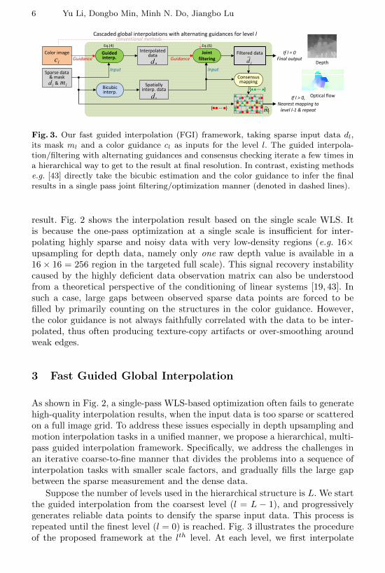
Fig. 3. Our fast guided interpolation (FGI) framework, taking sparse input data dl,its mask ml and a color guidance cl as inputs for the level l. The guided interpola-tion/filtering with alternating guidances and consensus checking iterate a few times ina hierarchical way to get to the result at final resolution. In contrast, existing methodse.g. [43] directly take the bicubic estimation and the color guidance to infer the finalresults in a single pass joint filtering/optimization manner (denoted in dashed lines).

result. Fig. 2 shows the interpolation result based on the single scale WLS. Itis because the one-pass optimization at a single scale is insufficient for inter-polating highly sparse and noisy data with very low-density regions (e.g. 16×upsampling for depth data, namely only one raw depth value is available in a16× 16 = 256 region in the targeted full scale). This signal recovery instabilitycaused by the highly deficient data observation matrix can also be understoodfrom a theoretical perspective of the conditioning of linear systems [19, 43]. Insuch a case, large gaps between observed sparse data points are forced to befilled by primarily counting on the structures in the color guidance. However,the color guidance is not always faithfully correlated with the data to be inter-polated, thus often producing texture-copy artifacts or over-smoothing aroundweak edges.

3 Fast Guided Global Interpolation

As shown in Fig. 2, a single-pass WLS-based optimization often fails to generatehigh-quality interpolation results, when the input data is too sparse or scatteredon a full image grid. To address these issues especially in depth upsampling andmotion interpolation tasks in a unified manner, we propose a hierarchical, multi-pass guided interpolation framework. Specifically, we address the challenges inan iterative coarse-to-fine manner that divides the problems into a sequence ofinterpolation tasks with smaller scale factors, and gradually fills the large gapbetween the sparse measurement and the dense data.

Suppose the number of levels used in the hierarchical structure is L. We startthe guided interpolation from the coarsest level (l = L − 1), and progressivelygenerates reliable data points to densify the sparse input data. This process isrepeated until the finest level (l = 0) is reached. Fig. 3 illustrates the procedureof the proposed framework at the lth level. At each level, we first interpolate


the sparse input dl4 by performing the WLS optimization using a corresponding

color image cl as the guidance and also a simple bicubic interpolation technique,respectively. Then, another WLS is applied with the interpolated dense data d∗from the first WLS interpolation output as the guidance and the bicubic inter-polated map as the input signal. Finally, we select reliable points via consensuschecking, and pass the augmented data points to the next level l − 1.

For a sparse data input, we use a mask ml (l = 0, ..., L−1) to denote the dataobservation or constraint map whose elements are 1 for pixels with valid dataand 0 otherwise. At each level, we upsample the signal by a factor of 2. We alsopre-compute a downsampled color image cl for each level from a high resolutioncolor image c such that c0 = c, cl = cl−1 ↓ (l = 1, 2, . . . , L− 1), where ↓ denotesa downsampling operation by a factor of 2. A sparse input at the starting level(l = L − 1) can be depth data from a low resolution depth map or irregularsparse motion matches mapped from descriptor matching methods (e.g. [39]).

3.1 Cascaded Filtering with Alternating Guidances

For a progressively densified input data dl at a certain level l, our techniqueperforms two cascaded WLS by alternating the color image cl and an interme-diate interpolated depth or flow map d∗ as the guidance (see Fig. 3). For thefirst WLS-based interpolation using the color guidance, the sparse input datadl is quickly densified at the current scale. In this pass, the sparse data is in-terpolated in accordance with the color structures. This process may introducespurious structures to the interpolated data d∗ (e.g. texture-copying effects) dueto inconsistent structures between the color and sparse input depth/motion data,but d∗ interpolated from the sparse input data dl contains much weaker texturepatterns than the original guidance signal cl (see d∗ in Fig. 4). Therefore, wepropose to append the second modified WLS smoothing step using the newlyinterpolated data d∗ as the guidance. During this second pass, the WLS opti-mization is solved with a more faithful guidance of the same modality (i.e. d∗rather than cl), while being subject to dense data constraints from the bicubic-upsampled data d◦. We find this cascaded scheme effectively addresses the po-tential structure inconsistency between the sparse input data and the guidanceimage, while preserving true depth or motion discontinuities (see Fig. 2 & 4).1st WLS using cl as the guidance. When the sparse input data dl and theguidance color image cl are given at the lth level, the first WLS step, minimizingthe following objective, is invoked to obtain an intermediate dense output d∗:

E(d∗) = (d∗ − dl)>Ml(d∗ − dl) + λ1 d>∗ Acld∗ , (4)

where Ml is a diagonal matrix with its elements given by the mask map ml. Acl

denotes the spatially varying Laplacian matrix defined by the guidance image clat the lth level. Unlike the image smoothing task using a dense input in (2), theinput data dl is sparse, and thus directly minimizing it in a separable manner

4 Hereinafter we denote the corresponding vectorized form of d as d.


2~d 1

~d

0~d

*d

*d

*d

One‐pass WLS Ground truth

l=2 l=2 l=1 l=1

l=0 l=0

Guidance

Ground truth = our result

Fig. 4. Comparison of the 1D scanline results obtained by our cascaded WLS stepsover three levels l = 2, 1, 0, and that obtained by the one-pass WLS. In all the subplots(right), the corresponding color signal is in olive green, while other kinds of signals arein different colors. The same is observed for optical flow interpolation.

leads to unstable results. Instead, as in [31, 18], we compute the solution d∗ with

d∗(p) =((E + λAcl)

−1dl)(p)

((E + λAcl)−1ml)(p)

, (5)

where ml denotes the corresponding vectorized form of ml. The WLS is appliedtwice to dl and ml, respectively.2nd WLS using d∗ as the guidance. Here, the input data d◦ is obtainedby a bicubic interpolation of dl at the lth level, and the guidance signal is theintermediate interpolated data d∗. A similar objective is minimized as:

E(dl) = (dl − d◦)>(dl − d◦) + λ2d

>l Ad∗ dl , (6)

where Ad∗ denotes the Laplacian matrix defined by d∗. Note that the input datad◦ is dense in this pass, while dl is sparse in the 1st WLS.

To give more intuitions of the proposed cascaded filtering process with al-ternating guidances, we show in Fig. 4 the processing results for one scanline(extracted from real images in Fig. 2): d∗ and dl from the 1st and 2nd WLS steps,iterating from l = 2 down to l = 0. Over the iterations, both of our intermediateguidance signal d∗ and the 2nd WLS output dl are progressively improved, withthe final output d0 close to the ground truth. In contrast, the result of applyingthe one-pass WLS contains spurious color structures (though attenuated), whichare mistakenly transferred from highly-varying texture regions.

It is worth noting the difference from the rolling guidance filter (RGF) [44],though using progressively improved guidance signals appears somewhat related.First, they are developed for different objectives: RGF focuses on removing smallstructural details for image smoothing, but our FGI tackles notorious interpola-tion issues such as inconsistent structures between a color guidance image and asparse depth or flow map. Second, RGF needs to carefully set the target scale pa-rameter for its Gaussian prefiltering, but inconsistent structures across differentsignal modalities are often not small. Third, RGF has the limitation of bluntingimage corners, while FGI preserves important depth or motion structures.


3.2 Consensus-Based Data Point Augmentation

Thanks to the hierarchical interpolation framework, the proposed algorithm isnot required to generate a fully dense data set for any intermediate level, whichmay propagate some unreliable data points to the next level otherwise. There-fore, we can be prudent in selecting reliable new data points to augment the inputsparse data set dl. As the last consistency checking in this current iteration l, weevaluate the consensus between the interpolated data points dl obtained fromalternating guidance filtering and the data points d◦ from a direct bicubic inter-polation. In fact, without using the color guidance in the spatial interpolationprocess, d◦ is free from color texture copying artifacts, though it has difficultiesin restoring sharp edges/structures. Therefore, if we impose a consensus check-ing in the interpolated data between d◦ and dl, those unwanted color texturepatterns in dl will not be chosen. This cautious design helps preventing thosenew data points of low confidence (e.g. undesired texture-copy patterns) fromcontaminating the next interpolation process.

Our consensus-based data point augmentation proceeds in a non-overlappingpatch fashion. For each pixel q in the patch we check the consistency betweenthe interpolated data points dl and the bicubic upsampled data points d◦ asδ(q) = ‖dl(q)−d◦(q)‖. After the consensus checking we pick the most consistentdata location in the current patch (i.e. with the smallest δ(q) and also smallerthan a preset threshold τ) and add this location to the data mask map ml. Fig. 3illustrates this data augmentation process by denoting new data points in ma

l

as green triangles and initial sparse data points ml as red dots. By selectingat most one new data point in each patch, we intend to avoid propagating theinterpolation error to the next level. We use 2× 2 patches in this paper.

3.3 Computational Complexity

The computational cost is mainly from solving the WLS objective in (3), as otherparts have marginal computational overhead. To compare the complexity of ourmethod with a single scale WLS based interpolation, we first count how manytimes the linear system is solved in both methods. In each level, the WLS basedguided interpolation of (4) requires solving the linear system twice as in (5)–one for the input signal and one for the binary index signal, after which the finalsolution is obtained by an element-wise division . The WLS of (6) needs to solvethe linear system once as its input d◦ is dense. Thus, the linear system solveris applied 3 times at each level of our method. Since the interpolation grid isprogressively rescaled with a factor of 2, our hierarchical framework increases thetotal computational complexity at most by 1/(1 − 1/4) = 4/3. One can expectour hierarchical approach to have (2+1)×4/3 = 4 passes of executing the linearsystem solver, while the single scale WLS based interpolation needs 2 passes.

4 Experiments

We perform our experiments on a PC with Intel Xeon CPU (3.50 GHz) and 16GB RAM. The implementation was in C++. For minimizing the WLS objective


1.311.83

2.60

3.76

0.791.23

2.05

3.29

0.79 1.00

1.61

2.67

0.650.92

1.41

2.31

0

1

2

3

4

2x 4x 8x 16x

Dep

th Upsam

ling Error (MAD)

Single scale WLS+Cascaded filtering with alternating guidances ‐ single scale (Sec. 3.1)+Hierarchical process+Consensus‐based data point augmentation (Sec. 3.2)

Fig. 5. The effect of each component of our pipeline evaluated on depth upsampling.

Table 1. Quantitative comparison (MAD) on ToF-like synthetic datasets [43]. Bestresults are in bold, and the second best are underlined.

MethodArt Book Moebius Reindeer Laundry Dolls Average

2x 4x 8x 16x 2x 4x 8x 16x 2x 4x 8x 16x 2x 4x 8x 16x 2x 4x 8x 16x 2x 4x 8x 16x 2x 4x 8x 16x

Bicubic 3.52 3.84 4.47 5.72 3.30 3.37 3.51 3.82 3.28 3.36 3.50 3.80 3.39 3.52 3.82 4.45 3.35 3.49 3.77 4.35 3.28 3.34 3.47 3.72 3.35 3.49 3.76 4.31JGF [28] 2.36 2.74 3.64 5.46 2.12 2.25 2.49 3.25 2.09 2.24 2.56 3.28 2.18 2.40 2.89 3.94 2.16 2.37 2.85 3.90 2.09 2.22 2.49 3.25 2.17 2.37 2.82 3.85GF [21] 1.49 1.97 3.00 4.91 0.8 1.22 1.95 3.04 1.18 1.90 2.77 3.55 1.29 1.99 2.99 4.14 1.28 2.05 3.04 4.10 1.19 1.94 2.80 3.50 1.21 1.85 2.76 3.87CLMF0[30] 1.19 1.77 2.95 4.91 0.90 1.48 2.38 3.36 0.87 1.44 2.32 3.3 0.96 1.56 2.54 3.85 0.94 1.55 2.50 3.81 0.96 1.54 2.37 3.25 0.97 1.56 2.51 3.75MRF+nlm[34] 1.69 2.40 3.60 5.75 1.12 1.44 1.81 2.59 1.13 1.45 1.95 2.91 1.20 1.60 2.40 3.97 1.28 1.63 2.20 3.34 1.14 1.54 2.07 3.02 1.26 1.68 2.34 3.60TGV[17] 0.82 1.26 2.76 6.87 0.50 0.74 1.49 2.74 0.56 0.89 1.72 3.99 0.59 0.84 1.75 4.40 0.61 1.59 1.89 4.16 0.66 1.63 1.75 3.71 0.62 1.16 1.89 4.31AR [43] 0.76 1.01 1.70 3.05 0.47 0.70 1.15 1.81 0.46 0.72 1.15 1.92 0.48 0.80 1.29 2.02 0.51 0.85 1.30 2.24 0.59 0.91 1.32 2.08 0.55 0.83 1.32 2.19WLS [31] 1.34 1.90 2.95 4.63 1.25 1.70 2.39 3.29 1.34 1.92 2.66 3.56 1.47 2.05 2.82 4.09 1.11 1.55 2.24 3.49 1.34 1.85 2.55 3.50 1.31 1.83 2.60 3.76FGI (ours) 0.79 1.17 2.01 3.65 0.58 0.80 1.13 1.75 0.58 0.80 1.15 1.71 0.65 0.89 1.36 2.37 0.65 0.97 1.49 2.43 0.67 0.91 1.31 1.95 0.65 0.92 1.41 2.31

function, we use the FGS [31] solver provided on its project site [1] (also possibleto use its OpenCV 3.1 function [2]). We will make our code publicly available. Inall the experiments, we fix the smooth weights λ1 = 30.02, λ2 = 10.02, and theconsensus checking threshold τ = 15(depth)/1(motion). For the affinity weightwp,q(g) in (1), we follow [31] to set wp,q(g) = exp(−‖gp−gq‖/σ) with σ = 0.005.

4.1 Depth Upsampling Results

Pipeline Validation. First, we present a quick study on our pipeline designgiven in Sec. 3 on the depth upsampling task with the dataset provided by [43].Starting from the single pass WLS based interpolation, we gradually add in newfeatures until getting to our full pipeline. The comparison of the average errorin the upsampled depth maps is plotted in Fig. 5. As can be seen, adding thecascaded filtering with one more WLS using alternating guidance in the singlescale leads to lower errors in depth upsampling. Note, however, the gain fromthis step is almost fixed for all upsampling factors. To handle more challengingcases with high upsampling rates (e.g. 8 or 16), employing the hierarchical pro-cess yields better results, which meets our expectation. The last module tested isthe consensus-based data point augmentation. This strategy further reduces theupsampling errors. Overall, our whole pipeline obtains much better depth up-sampling results than the direct single pass WLS interpolation (see also Fig. 2).

We now evaluate the performance of depth upsampling with different edge-aware smoothing filters. We take the popular GF [21] for this test. The averageerror of a single pass interpolation with GF are 1.31/1.54/2.04/3.12 for upscalingrate 2/4/8/16. When using our pipeline with GF (i.e. replacing all the WLS stepswith GF), the results are 1.06/1.21/1.63/2.59. The improvements confirm thatour framework is generic to other edge-aware filtering techniques. We chooseFGS [31] as our fundamental block for its best efficiency and accuracy.


Table 2. Average runtime (in sec) to upsample by 4× an input depth map 272× 344.

Method MRF+nlm[34] TGV [17] AR [43] GF [21] CLMF0 [30] WLS [31] FGI (ours)Runtime(s) 170 420 900 1.26 2.4 0.32 0.65

Ground truth/Color MRF+nlm [34] JGF [28] TGV [17] AR [43] FGI(ours)

Fig. 6. Visual comparison on 8× upsampling results and error maps of Art and Moebiusfrom the ToF-like synthetic dataset [43]. (Best viewed in electronic version.)

Results on ToF-like synthetic datasets [43]. We evaluate the proposed FGImethod on a ToF depth upsampling task using the synthetic datasets providedby [43]. They used six datasets from Middlebury benchmarks [3] to simulateToF-like depth degradation by adding noise and performing downsampling withfour different scales, i.e. 2, 4, 8, 16. Our FGI uses L = 1, 2, 3, 4 levels architec-ture for four different upsampling scales. Table 1 reports the Mean AbsoluteDifference (MAD) between ground truth depth maps and the results by variousdepth upsampling methods including ours. The proposed method clearly out-performs several existing methods like CLMF0 [30], JGF [28], MRF+nlm [34]and TGV [17] that used different color-guided upsampling or optimization tech-niques. Our method also yields much smaller error rates than the single-passWLS interpolation, validating the effectiveness of our hierarchical structure. Fi-nally, when compared with the state-of-the-art AR method [43] over all testimage sets for challenging higher upsampling rates (8, 16), our FGI actuallyyields more accurate depth maps on half of them, i.e. Book, Moebius, and Dolls.Though slightly worse than AR [43] in terms of the MAD, our FGI is the secondbest among all leading methods, and runs over 1000× faster than AR [43].

Table 2 summarizes the runtime of various methods whose source codes areavailable and timed on our PC. Generally, the methods using global optimiza-tions e.g. MRF+nlm [34], TGV [17] and AR [43] come with much higher compu-tational costs. GF [21] and CLMF0 [30], as local filtering methods, take less time


Table 3. Quantitative results (MAD in millimeter) on the real ToFMark datasets [4].

Bicubic JBU [22] GF [21] JGF [28] TGV [17] FGI (ours)Books 16.23 16.03 15.74 17.39 12.36 13.03Devil 16.66 27.57 27.04 19.02 14.68 15.09Shark 17.78 18.79 18.21 18.17 15.29 15.82

JGF [28] TGV [17] Ours JGF [28] TGV [17] Ours

Fig. 7. Depth upsampling results and error maps of Books and Devil in ToFMark [4].

to upsample a depth map, but they are still slower than our fast optimization-based method. The single-pass WLS with the FGS solver [31] takes only 0.32s.Our FGI also takes advantage of the FGS solver [31] and is fast. Since we use dif-ferent numbers of levels for different upsample rates, its runtimes vary slightlyfor them, i.e. 0.51/0.65/0.69/0.73s for upscaling rate 2/4/8/16. The runtimeresults of the single-scale WLS and our FGI are also consistent with the com-plexity analysis in Sec. 3.3. Another efficient method JGF [28] reports 0.33s inupsampling 8× to 0.4M depth images, but FGI takes 0.19s on the same size.

Fig. 6 shows two visual comparisons of depth maps upsampled by differentmethods on this synthetic dataset. The results of MRF+nlm [34] fail to recoverthe depth for the thin structures in the Art case and show texture-copy artifactsin the Moebius case. The depth maps by JGF [28] contain noticeable noise asit is designed without any consideration of the noise issue from depth sensors.A separate noise removal process may be applied before JGF to solve the noiseproblem while our method (like most leading depth upsampling methods) doesnot require such a separate pre-processing. It is clearly observed that among allmethods compared, AR [43] and our FGI recover accurate depths in homoge-neous regions and along depth boundaries, and preserve thin structures betterthan other methods. More visual results are given in the supplemental materials.

Results on the ToFMark datasets [4]. We further test on the ToFMarkdatasets [4] provided in the TGV paper [17] that contain three real ToF depthand intensity image pairs i.e. Books, Devil, Shark. The ToF depth maps of spatialresolution 120×160 are real depth values in millimeter (mm), while the intensityimages are of size 610× 810. Table 3 presents the quantitative results measuredby MAD in mm. Our method outperforms prevailing methods like JBU [22],GF [21], JGF [28], and obtains performance quite close to TGV [17]. Fig. 7 showsthe visual comparison of different methods. The depth recovered by JGF [28]again exhibits noticeable noise, while the results of TGV [17] and ours are muchsharper and cleaner, but our FGI runs about 650× faster than TGV [17].


Table 4. Performance comparison (EPE) on the Sintel training set [9].

Method Clean Final Runtime Method Clean Final RuntimeEpic-NW [35] 3.17 4.55 0.80s WLS [31] 3.23 4.68 0.21sEpic-LA [35] 2.65 4.10 0.94s FGI (ours) 2.75 4.14 0.39s

Epic‐LA

Ours

Inpu

t

Ground truth Ground truth Ground truth

(a) Weak edge in color guidance (b) Sparsely scattered points (c) Extrapolation

Fig. 8. Optical flow fields interpolated by our method and Epic-LA [35] on the Sinteldatasets on three challenging cases. Please refer to Sec. 4.2 for more analysis.

4.2 Motion Field Interpolation for Optical Flow

We evaluate our motion interpolator using the MPI Sintel dataset [9], a modernoptical flow evaluation benchmark with large displacement flow and complexnon-rigid motions. The evaluation is conducted on two types of rendered frames,i.e. clean pass and final pass, where the final pass includes more complex effectssuch as specular reflections, motion blur, defocus blur, and atmospheric effects.We evenly sampled 331 frames from the whole training set and used them forevaluation and the rest of the frames were used to choose the best parameters.The number of levels L in the hierarchical structure is fixed to 3.

To generate a set of sparse matches, we adopt a leading descriptor-basedmatching algorithm – DeepMatching [39], one of the top methods on the Sin-tel benchmark. We perform the same match pruning step as EpicFlow [35] toremove unreliable matches, so the set of sparse matches used in our methodand EpicFlow are exactly the same. After the pruning step, we usually can get5000∼6000 reliable matches on 436×1024 color frames. This motion interpolationtask from sparse data with about 1% density is challenging, especially consid-ering the data points are not uniformly distributed. Note that besides [39], ourframework is flexible to take in other choices of reliable motion matches e.g. [6].

For performance comparison on the 331 frames , we test with the single passWLS [31], and also with both the locally-weighted affine (LA) and Nadaraya-Watson (NW) interpolators of EpicFlow [35], denoted as Epic-LA and Epic-NW.Table 4 reports the performance of these methods. Compared with the single passWLS, our FGI shows improvements in the sparse-to-dense interpolation results,again demonstrating the effectiveness of our pipeline. Our method achieves aquantitative performance better than EpicFlow-NW and very close to EpicFlow-LA, while reducing the runtime of the interpolation process by over 50%.


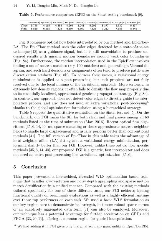
Table 5. Performance comparison (EPE) on the Sintel testing benchmark [9].

FlowFields[6] EpicFlow[35] PH-Flow[42] FGI (ours) Deep+R[14] SPM-BP[27] DeepFlow[39] PCA-Layers[40] MDP-Flow2[41]

Clean 3.748 4.115 4.388 4.664 5.041 5.202 5.377 5.730 5.837Final 5.810 6.285 7.423 6.607 6.769 7.325 7.212 7.886 8.445

Fig. 8 compares optical flow fields interpolated by our method and EpicFlow-LA. The EpicFlow method uses the color edges detected by a state-of-the-arttechnique [13] as a guidance signal, but it is still unavoidable to produce un-desired results with missing motion boundaries around weak color boundaries(Fig. 8a). Furthermore, the motion interpolation used in the EpicFlow involvesfinding a set of nearest matches (e.g. 100 matches) and generating a Voronoi di-agram, and such hard decisions or assignments often tend to produce patch-wisediscretization artifacts (Fig. 8b). To address these issues, a variational energyminimization is applied as a post-processing, but such problems are not fullyresolved due to the local minima of the variational approach. More seriously, inextremely low density regions, it often fails to densify the flow map properly dueto its essentially localized, approximated geodesic propagation strategy (Fig. 8c).In contrast, our approach does not detect color edges to directly guide the inter-polation process, and also does not need an extra variational post-processing5

thanks to the global optimization formulation using a hierarchical strategy.Table 5 reports the quantitative evaluation on the Sintel test set [5]. On the

benchmark, our FGI ranks the 8th for both clean and final passes among all 63methods listed at the time of submission (Mar. 2016). Recent optical flow algo-rithms [35, 6, 14, 40] use sparse matching or dense approximate nearest neighborfields to handle large displacement and usually perform better than conventionalmethods [41]. The full version of EpicFlow in this table takes the advantage oflocal-weighted affine (LA) fitting and a variational energy minimization, per-forming slightly better than our FGI. However, unlike these optical flow specificmethods [35, 6, 14, 40], our proposed FGI is a generic, fast interpolator and doesnot need an extra post processing like variational optimization [35, 6].

5 Conclusion

This paper presented a hierarchical, cascaded WLS-optimization based tech-nique that handles low-resolution and noisy depth upsampling and sparse motionmatch densification in a unified manner. Compared with the existing methodstailored specifically for one of these different tasks, our FGI achieves leadingfunctional quality on benchmark evaluations as well as a highly efficient runtimeover those top performers on each task. We used a basic WLS formulation asour key engine here to demonstrate its strength, but more robust sparse normsor an adaptively aggregated data term [31] can also be employed. Moreover,our technique has a potential advantage for further acceleration on GPUs andFPGA [33, 20, 11], offering a common engine for guided interpolation.

5 We find adding it in FGI gives only marginal accuracy gain, unlike in EpicFlow [35].


References

1. Https://sites.google.com/site/globalsmoothing/2. Http://docs.opencv.org/master/da/d17/group ximgproc filters.html3. http://vision.middlebury.edu/stereo/4. http://rvlab.icg.tugraz.at/tofmark/5. http://sintel.is.tue.mpg.de/results6. Bailer, C., Taetz, B., Stricker, D.: Flow fields: Dense correspondence fields for

highly accurate large displacement optical flow estimation. In: ICCV (2015)7. Bao, L., Song, Y., Yang, Q., Yuan, H., Wang, G.: Tree filtering: Efficient structure-

preserving smoothing with a minimum spanning tree. IEEE Trans. on Image Pro-cessing 23(2), 555–569 (2014)

8. Brox, T., Bregler, C., Malik, J.: Large displacement optical flow. In: CVPR (2009)9. Butler, D.J., Wulff, J., Stanley, G.B., Black, M.J.: A naturalistic open source movie

for optical flow evaluation. In: ECCV (2012)10. Chan, D., Buisman, H., Theobalt, C., Thrun, S.: A noise-aware filter for real-time

depth upsampling. In: ECCV Workshop (2008)11. Chaurasia, G., Ragan-Kelley, J., Paris, S., Drettakis, G., Durand, F.: Compiling

high performance recursive filters. In: High Performance Graphics (2015)12. Diebel, J., Thrun, S.: An application of markov random fields to range sensing. In:

NIPS (2005)13. Dollar, P., Zitnick, C.L.: Structured forests for fast edge detection. In: ICCV. IEEE

(2013)14. Drayer, B., Brox., T.: Combinatorial regularization of descriptor matching for op-

tical flow estimation. In: BMVC (2015)15. Elad, M.: On the origin of the bilateral filter and ways to improve it. IEEE Trans.

on Image Processing 11(10), 1141–1151 (2002)16. Farbman, Z., Fattal, R., Lischinski, D., Szeliski, R.: Edge-preserving decompo-

sitions for multi-scale tone and detail manipulation. ACM Trans. Graph. 27(3)(2008)

17. Ferstl, D., Reinbacher, C., Ranftl, R., Ruther, M., Bischof, H.: Image guided depthupsampling using anisotropic total generalized variation. In: ICCV (2013)

18. Gastal, E.S.L., Oliveira, M.M.: Domain transform for edge-aware image and videoprocessing. ACM Trans. Graph. 30(4) (2011)

19. Golub, G.H., Loan, C.F.V.: Matrix Computations. Johns Hopkins University Press(1996)

20. Greisen, P., Runo, M., Guillet, P., Heinzle, S., Smolic, A., Kaeslin, H., Gross, M.:Evaluation and FPGA implementation of sparse linear solvers for video processingapplications. IEEE Trans. on Circuits and Systems for Video Technology 23(8),1402–1407 (Aug 2013)

21. He, K., Sun, J., Tang, X.: Guided image filtering. In: ECCV (2010)22. Kopf, J., Cohen, M.F., Lischinski, D., Uyttendaele, M.: Joint bilateral upsampling.

ACM Trans. Graph. 26(3) (2007)23. Koutis, I., Miller, G.L., Tolliver, D.: Combinatorial preconditioners and multilevel

solvers for problems in computer vision and image processing. CVIU 115(12), 1638–1646 (2011)

24. Krishnan, D., Fattal, R., Szeliski, R.: Efficient preconditioning of laplacian matricesfor computer graphics. ACM Trans. Graph. (2013)

25. Lang, M., Wang, O., Aydin, T.O., Smolic, A., Gross, M.H.: Practical temporalconsistency for image-based graphics applications. ACM Trans. Graph. 31(4), 34–1 (2012)


26. Leordeanu, M., Zanfir, A., Sminchisescu, C.: Locally affine sparse-to-dense match-ing for motion and occlusion estimation. In: ICCV (2013)

27. Li, Y., Min, D., Brown, M.S., Do, M.N., Lu, J.: SPM-BP: Sped-up patchmatchbelief propagation for continuous MRFs. In: ICCV (2015)

28. Liu, M.Y., Tuzel, O., Taguchi, Y.: Joint geodesic upsampling of depth images. In:CVPR (2013)

29. Lu, J., Min, D., Pahwa, R.S., Do, M.N.: A revisit to MRF-based depth map super-resolution and enhancement. In: ICASSP (2011)

30. Lu, J., Shi, K., Min, D., Lin, L., Do, M.N.: Cross-based local multipoint filtering.In: CVPR (2012)

31. Min, D., Choi, S., Lu, J., Ham, B., Sohn, K., Do, M.N.: Fast global image smoothingbased on weighted least squares. IEEE Trans. on Image Processing 23(12), 5638–5653 (2014)

32. Min, D., Lu, J., Do, M.N.: Depth video enhancement based on weighted modefiltering. IEEE Trans. on Image Processing 21(3), 1176–1190 (2012)

33. Nehab, D., Maximo, A., Lima, R.S., Hoppe, H.: GPU-efficient recursive filteringand summed-area tables. ACM Trans. Graph. 30(6), 176:1–176:12 (Dec 2011)

34. Park, J., Kim, H., Tai, Y.W., Brown, M.S., Kweon, I.: High quality depth mapupsampling for 3D-ToF cameras. In: ICCV (2011)

35. Revaud, J., Weinzaepfel, P., Harchaoui, Z., Schmid, C.: EpicFlow: Edge-preservinginterpolation of correspondences for optical flow. In: CVPR (2015)

36. Shen, X., Zhou, C., Xu, L., Jia, J.: Mutual-structure for joint filtering. In: ICCV(2015)

37. Talebi, H., Milanfar, P.: Nonlocal image editing. IEEE Trans. on Image Processing23(10), 4460–4473 (2014)

38. Tomasi, C., Manduchi, R.: Bilateral filtering for gray and color images. In: IEEEInt. Conf. on Computer Vision. pp. 839–846 (1998)

39. Weinzaepfel, P., Revaud, J., Harchaoui, Z., Schmid, C.: DeepFlow: Large displace-ment optical flow with deep matching. In: ICCV (2013)

40. Wulff, J., Black, M.J.: Efficient sparse-to-dense optical flow estimation using alearned basis and layers. In: CVPR (2015)

41. Xu, L., Jia, J., Matsushita, Y.: Motion detail preserving optical flow estimation.TPAMI 34(9), 1744–1757 (2012)

42. Yang, J., Li, H.: Dense, accurate optical flow estimation with piecewise parametricmodel. In: CVPR (2015)

43. Yang, J., Ye, X., Li, K., Hou, C., Wang, Y.: Color-guided depth recovery from RGB-D data using an adaptive autoregressive model. IEEE Trans. on Image Processing23(8), 3443–3458 (2014)

44. Zhang, Q., Shen, X., Xu, L., Jia, J.: Rolling guidance filter. In: ECCV (2014)

Fast Guided Global Interpolation for Depth and...

Documents

Transcript of Fast Guided Global Interpolation for Depth and...