Eurographics Symposium on Geometry Processing 2012Eitan Grinspun and Niloy Mitra(Guest Editors)

Volume 31 (2012), Number 5

Fast and Robust Normal Estimation for Point Clouds

with Sharp Features

Alexandre Boulch1 and Renaud Marlet1

1 Université Paris-Est, LIGM (UMR CNRS), Center for Visual Computing, Ecole des Ponts ParisTech6-8 av. Blaise Pascal, 77455 Marne-la-Vallée, France

Abstract

This paper presents a new method for estimating normals on unorganized point clouds that preserves sharp fea-

tures. It is based on a robust version of the Randomized Hough Transform (RHT). We consider the filled Hough

transform accumulator as an image of the discrete probability distribution of possible normals. The normals we

estimate corresponds to the maximum of this distribution. We use a fixed-size accumulator for speed, statistical ex-

ploration bounds for robustness, and randomized accumulators to prevent discretization effects. We also propose

various sampling strategies to deal with anisotropy, as produced by laser scans due to differences of incidence.

Our experiments show that our approach offers an ideal compromise between precision, speed, and robustness:

it is at least as precise and noise-resistant as state-of-the-art methods that preserve sharp features, while being

almost an order of magnitude faster. Besides, it can handle anisotropy with minor speed and precision losses.

Categories and Subject Descriptors (according to ACM CCS): I.3.5 [Computer Graphics]: Computational Geometryand Object Modeling—

1. Introduction

Numerous algorithms rely on the quality of normal estima-tion in point clouds, such as point-based rendering [RL00],surface reconstruction [ÖGG09], 3D piecewise-planar re-construction [CLP10] and primitive extraction [SWK07].

For this, regression methods are the most common. Hoppeet al. [HDD∗92] estimate normals approximating a tangentplane with a regression that is computed efficiently by prin-cipal component analysis (PCA). Other surfaces have beenused too, e.g., spheres [GG07] or jets (a truncated Taylor ex-pansion of a surface expression) such as quadrics [CP03].Regression methods are robust to noise, although they canbe improved in that respect with adaptive neighborhoodsizes [MNG04], but they are sensitive to outliers. More re-cent work handles both noise and outliers [GG07,HLZ∗09,YLL∗07]. However, all regression-based techniques tend tosmooth sharp features, and thus fail to correctly estimatenormals near edges (see Figure 1). The estimation qualityalso depends a lot on the size of the neighborhood usedfor regression: larger neighborhoods are needed to deal withnoise, but they make sharp features even smoother.

Another class of methods is based on a preliminary nor-mal estimation, which is improved. Algorithms such as

Figure 1: Reconstructed normals of a corner with Least

Square Regression (left) and our method (right).

Moving Least Squares (MLS) [ABCO∗01], adaptive ver-sions [PKKG03], or robust Local Kernel Regression (LKR)[ÖGG09] compute an implicit surface and estimate normalsas the gradient of the surface. They can retrieve sharp fea-tures, but they depend on a reliable prior estimation of inputnormals. Bilateral filtering [JDZ04] also preserves sharp fea-tures while smoothing even regions, but it can be slow andthe quality relies on that of input normals too.

Other approaches directly estimate normals with a methodthat does not oversmooth edges. Dey’s method [DG06] re-lies on the construction of a Voronoï diagram and the searchof the furthest vertex of the Voronoï cell. This method pre-serves sharp features and can deal with density variation.But it is quite sensitive to noise (and does not handle sur-

c© 2012 The Author(s)

Computer Graphics Forum c© 2012 The Eurographics Association and Blackwell Publish-

ing Ltd. Published by Blackwell Publishing, 9600 Garsington Road, Oxford OX4 2DQ,

UK and 350 Main Street, Malden, MA 02148, USA.

A. Boulch & R. Marlet / Fast and Robust Normal Estimation for Point Clouds with Sharp Features

Figure 2: Laser scan of room, highlights of a corner with

density anisotropy and a beveled edge.

Figure 3: Reconstructed normals of a corner with sharp

density variation: Li et al.’s algorithm (left) and ours (right).

face boundaries). Alliez et al. [ACSTD07] address this issuewith a Voronoï-PCAmethod that provides some control oversmoothness. More recently, both noise and sharp featureshave been treated explicitly by Li et al. [LSK∗10], com-bining a robust local noise estimation and a RANSAC-likemethod that is parameterized by the estimated noise scale. Ithandles well noise and outliers. But it is not very fast (typi-cally around half an hour for 1.5 million points). Besides, itdoes not address variation of density at edges.

Yet, sampling anisotropy is common in laser data, es-pecially when scanning objects with access constraints orabrupt variations, such as buildings. First, the scanning de-vice may not space samples evenly. For instance, lasers witha rotating head that are used to scan their surroundings sys-tematically oversample the upper polar region (vertical di-rection), compared to the equatorial band (horizontal direc-tions), typically with a factor of one or two orders of mag-nitude. (The lower pole is generally occluded by the tri-pod support.) Second, even when device sampling is mostlyuniformly spaced, e.g., locally when focusing only on asmall area, the actual 3D spacing of the sampled data de-pends on the incidence of the laser on the surface. As man-made objects often present sharp features, a significant lo-cal anisotropy frequently appears in areas around edges. Buteven a smooth object shows sampling variations when thelaser beam is almost tangent to the surface. This is illus-trated in Figure 2 (left). Moreover, variations of density canalso appear in point clouds originating from photogramme-try, even on smooth surfaces, because of reconstruction er-rors and imprecision, e.g., due to specular or textureless sur-faces. (In our experiments with lasers and photogrammetry,we observed that noise was not isotropic either; it dependson the surface, in particular on the viewpoint incidence.) Yet,most normal estimation methods do not have any specific

treatment of anisotropy. This is illustrated in Figure 3, wherea variation of point density in two planes creates estimationerrors in the low-density area where they intersect.

We present a new method for estimating normals that ad-dresses the requirements of real data: sensitivity to sharpfeatures, robustness to noise, to outliers, and to samplinganisotropy, as well as computational speed to achieve scala-bility. This method is based on a fast and robust adaptationof the Randomized Hough Transform (RHT).

The Hough transform [Hou62] has been originally in-troduced to detect lines and arcs in bubble chamber pic-tures. Duda and Hart [DH72] discretize the space and in-troduced accumulators. The main idea of this transform isto change the data representation space such that the desiredshape accumulates in a way that is easy to detect [IK88].It has been successfully used in two dimensions to detectother primitives such as ellipses [TM78] or corners [Dav88].With the generalized Hough transform (GHT) [Bal87], Bal-lard shows that the method can also be applied to detectnon analytic features in images. The Hough transform hasbeen applied in many ways for detection and classification[Low04,GL09, BLK10,Oka09]. It generalizes to higher di-mensions and has been used in particular for 3D segmenta-tion, recognition and registration [KPW∗10, PWP∗11]. Thegeneral algorithm has also been modified and improved forspeed, robustness and precision. As going through all thedata may take too much time, Kiryati et al. [KEB91] proposea probabilistic version, consisting in observing only sub-sets. Xu et al. [XOK90,XO93] define a Randomized HoughTransform, where a point does not vote for all the primitivesto which it belongs; the vote is associated to a primitive com-puted from a subset of points. The criterion to stop pickingmore primitives is a user-defined, global condition.

As our objective is the estimation of a single normal ateach point, we adapt the Randomized Hough Transform tosearch for only one primitive. One original aspect of ourmethod is that we use a stop criterion inherited from robuststatistics to end exploring the space of primitives. This en-sures both speed and robustness to partial sampling. Robust-ness to density anisotropy is obtained by selecting primitivesas uniformly as possible in the neighborhood of the consid-ered point. We do not address the problem of orientating nor-mals, which can be done separately [HDD∗92,MdGD∗10].In the following, we first give a general overview of our nor-mal estimator (cf. §2) and describe our Robust RandomizedHough Transform (cf. §3). Then we explain how to computethe normals despite discretization (cf. §4) and anisotropy (cf.§5), and finally present our results (cf. §6).

2. Algorithm

Before describing our algorithm, let us consider the follow-ing simple situation. Let P be a point on a piecewise planarsurface and letNP be a neighborhood of P on this surface (asubsurface). There are two basic cases.

c© 2012 The Author(s)c© 2012 The Eurographics Association and Blackwell Publishing Ltd.

A. Boulch & R. Marlet / Fast and Robust Normal Estimation for Point Clouds with Sharp Features

• If P lies far from any edge or sharp feature, then pickingthree points in NP defines the planar patch that P lies on,and thus the normal (if the points are not collinear).

• If P lies near an edge partitioning the neighborhood NP

intoN1,P∪N2,P with P ∈N1,P, then picking three pointsin NP does not necessarily determine the right normal. Itdefines either the correct normal (if all points lie inN1,P),or the normal associated with the plane on the oppositeside of the edge (if all points lie in N2,P), or a “random”plane (if the points are not on the same side of the edge).

In the second case, as N1,P is likely to be larger than N2,P

since P ∈ N1,P is not exactly on the edge, the probabilityof picking the dominant plane and thus the correct normalis higher than the probability of picking the normal on theopposite edge side. When P is very close to the edge, drawntriples are likely to lie on both sides of the edge. However, asit leads to a “random” normal, the correct normal still is theone with the highest probability. This generalizes to situa-tions where P is close to several edges, including coincidentedges. This idea applies as well to a point cloud C in whichneighboring points NP are defined for any point P ∈ C.

Our method is a robust variant of this simple principle,to handle noise and outliers. For this, we sample as manyplanes as necessary to gain enough confidence that we canidentify the actual maximum of the probability density. Inpractice, we discretize the problem and fill a Hough accu-mulator until a normal can be confidently chosen based onthe most voted bin, with the following refinements:

• In the presence of noise and outliers, the discrete prob-ability distribution of possible normals is flatter, but theprincipal normal remains the one with the highest numberof votes. To ensure resistance to noise and outliers, we userobust statistical bounds on the number of triples to pick(cf. §3). Note that near collinearity need not be checkedbecause it is unlikely and would generate a “random” nor-mal anyway. On the contrary, checking collinearity at eachdrawing would be unnecessarily time consuming.

• If the surface is curved rather than piecewise planar, thediscrete probability distribution of possible normals isflatter too. However, as long as the surface can be lo-cally approximated with planes, the right normal staysthe most voted one. The size of the neighborhood impactsnormal estimation: it should be small enough for the pla-nar approximation hypothesis to hold, and large enoughfor noise to be averaged. (Neighborhoods are discussed inSection 5, together with anisotropy.)

• Using a Hough accumulator introduces discretization ar-tifacts. First, a single bin corresponds to a small range ofnormals (a cone). Rather than associating a fixed normalto a bin, we average the normals that vote for the bin. Sec-ond, we actually estimate the normal several times usingrandomized accumulators and use the best ones (cf. §4).

• To deal with density anisotropy, we propose a spatially-sensitive drawing scheme that comes in two versions, con-tinuous and precise, or discrete and fast (cf. §5).

3. Robust Randomized Hough Transform

The number of possible triples to pick can be huge, on theorder of |NP|

3. We thus want to consider only a subset, andwe want to stop sampling triples as soon as we are confidentenough that we can take a decision based on the empiricaldistribution in the accumulator. Using robust statistics tools,we determine a general upper bound on the number of triplesto draw, and possibly improve it when enough concentrationin a bin can be guaranteed. This defines a Robust Random-ized Hough Transform (RRHT) for estimating normals.

In the following, we consider that the M bins of the ac-cumulator follow a Bernoulli law with pm as parameter(the theoretical mean). Let T be the number of planes topick and let (Xm,t)m∈{1,...,M},t∈{1,...,T} be the independentand identically distributed random variables associated withbin m for plane t: Xm,t = 1 if plane t votes for bin m, other-wise Xm,t = 0. Finally, we note pm the empirical mean of theproportion of votes for bin m: pm = 1

T ∑Tt=1Xm,t .

Global upper bound. We want to stop drawing triples assoon as we are confident enough that the empirical distribu-tion is a good approximation of the actual distribution. Forthis, we want to bound the difference between the actual dis-tribution pm and the observed distribution pm.

Let α ∈]0,1[ be a probability threshold expressing theconfidence when comparing pm to pm, and let δ ∈]0,1[ bea distance. We wish to estimate the minimal number of sam-ples Tmin such that, for each bin m, the empirical mean pm isat most at distance δ from pm, with probability at least α:

P( maxm∈{1,...,M}

| pm− pm| ≤ δ)≥ α (1)

As Xm,t are i.i.d., Hoeffding’s inequality [Hoe63] applies:

∀m, P(| pm− pm| ≥ δ)≤ 2exp(−2δ2T 2

min

∑Tt=1(bt −at)2

) (2)

where [at ,bt ] is the interval where Xm,t lies, i.e., [0,1]. Thus:

P(| pm− pm| ≥ δ)≤ 2exp(−2δ2Tmin) (3)

As this is true for all m, we have:

P( maxm∈{1,...,M}

| pm− pm| ≥ δ)

= P(∃m ∈ {1, . . . ,M}, | pm− pm| ≥ δ) (4)

≤M

∑m=1

P(| pm− pm| ≥ δ) ≤ 2M exp(−2δ2Tmin) (5)

Hence:

P( maxm∈{1,...,M}

| pm− pm|< δ)≥ 1−2M exp(−2δ2Tmin) (6)

Now, considering equation (1), Tmin has to satisfy:

Tmin ≥1

2δ2ln(

2M

1−α) (7)

We may thus choose TR = 12δ2

ln( 2M1−α ) as an upper bound

on the number of triples to be drawn.

c© 2012 The Author(s)c© 2012 The Eurographics Association and Blackwell Publishing Ltd.

A. Boulch & R. Marlet / Fast and Robust Normal Estimation for Point Clouds with Sharp Features

Confidence interval. If we pick most of the time the samebin, we want to stop the selection operation. We use a con-fidence interval to identify it as the right bin to choose. Butit is actually enough to choose a bin that gets significantlymore votes than others, i.e., more votes than the second mostvoted bin. The above criterion only concerns the accuracy ofthe global distribution. What we want to estimate here is theconfidence interval of each pm. If the intervals of the twomost voted bins do not intersect, we are almost sure that themost voted bin will not change and we can stop picking moretriples.

According to the Central Limit Theorem, the random vari-able defined as

pm− pm√

pm(pm−1)/T

converges in distribution to a standard normal random vari-able N (0,1). Let r ∈]0,1[ be a confidence level and let z(r)be such that the integral of the Gaussian density between−z

and z is r. The confidence interval is then:

pm− z(r)

√

pm(1− pm)

T≤ pm ≤ pm+ z(r)

√

pm(1− pm)

T(8)

As pm ∈ [0,1], we have pm(1− pm)≤14 and thus:

pm−z(r)

2

√

1

T≤ pm ≤ pm+

z(r)

2

√

1

T(9)

Using, e.g., the confidence level r = 95%, we have z(r)≃ 2.In this context, if m1 is the most voted bin and m2 is thesecond most voted, we can stop sampling planes as soon asthe confidence intervals of these two bins do not intersect:

pm1 − pm2 ≥ 2

√

1

T(10)

This test may lower the global bound TR but does not replaceit (cf. §6). E.g., for a point lying very close to an edge, thetwo bins corresponding to the normal on each edge side arelikely to have similar probabilities. Confidence intervals thenrequire a large T before (10) is satisfied. In extreme cases,intervals always overlap and the condition is never fulfilled.

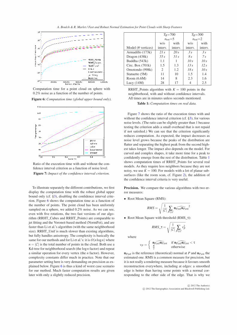
Accumulator shape. As we only estimate the normal di-rection, not the orientation, picking a triple of points definesa normal described by two angles (θ,φ), modulo π. It votesinto an accumulator that partitions half the unit sphere intosimilar bins. We use the spherical accumulator of Borrmannet al. [BELN11] that provides bins with similar area and al-lows easy and fast computation of bin indexes, given the nor-mal angles. This accumulator first divides the sphere accord-ing to the parallels, with same angle size. Then the slices(between two parallels) are divided into bins of nearly thesame area (cf. Fig. 4). We have chosen this accumulator af-ter also testing a geodesic sphere accumulator, that is moreisotropic but considerably slower for a limited precision im-provement.

nφ M

5 2310 8215 17120 29025 441

Figure 4: Accumulator shape & size for various nφ values.

With reference to Borrmann et al.’s paper, we define nφ asthe number of slices of the sphere in the z-axis and nθ = 2nφ

the number of bins at the equator. As we only estimate herethe normal direction, not the orientation, we use half of thebins in the accumulator. Figure 4 shows the value of the totalnumber of used bins M for several values of nφ:

4. Discretization issues

After plane sampling, the chosen normal is given by the mostvoted bin. However, rather than producing a discrete normal(one per bin in the accumulator), we average all the normalsthat voted for the chosen bin. From the implementation pointof view, sampled normals do not actually have to be memo-rized. It is enough to only record incrementally, for each bin,the sum of the normals that voted for the bin. When a bin ischosen, the sum of its contributing normals is renormalizedto lie on the unit sphere, yielding the final normal. (We havealso experimented memorizing for each bin the voting triplesof points, and computing the final normal as the regressionplane of the points in the most voted bin: the normal preci-sion is slightly better, but the running time is much longer.)

Using a discrete accumulator leads to other issues. First,there is a binning effect. If the main peak of the distributionof normals lies near a bin boundary, votes will be almostequally distributed between two (or more) adjacent bins. Af-ter a limited number of plane pickings, the actual peak maynot be in the most voted bin. The effect is stronger for noisydata as the distribution is flatter and votes are distributedinto more bins, that receive less votes on average. Second,bins are not isotropic. The accumulator of Borrmann et al.[BELN11] guarantees the area of all bins to be nearly equal,but their shape is different. For instance, polar bins are disks(caps) whereas equatorial bins are squares. A classic solu-tion to bin discretization would be for a normal to share partsof its vote in neighboring bins, but it does not answer thesecond problem. Both issues can be addressed by randomlyrotating the accumulator and running the algorithm severaltimes. The more rotations, the more precise the estimation.In practice, as few as 5 rotations are enough to compensatefor most discretization effects (cf. §6). From the implemen-tation point of view, it is more efficient to rotate the points,rather than rotating the accumulator itself.

As we run the algorithm several times, we get several nor-

c© 2012 The Author(s)c© 2012 The Eurographics Association and Blackwell Publishing Ltd.

A. Boulch & R. Marlet / Fast and Robust Normal Estimation for Point Clouds with Sharp Features

mals. Choosing the appropriate one depends of the sampledsurface and on applications. We propose three alternatives:

• RRHT_m: the produced normal is the mean of the nor-mals weighted by their number of votes. Compared to theother alternatives, it minimizes the root mean square er-ror, but it fails to estimate a plausible normal near edgesbecause of the smoothing effect of the mean.

• RRHT_b: the produced normal is the best one, i.e., themost voted one. Sharp features are well estimated, butsmooth surfaces may appear grainy.

• RRHT_c: we first cluster normals that are closed to eachother (within an angle threshold acluster) and then computethe average normal of the most voted cluster. Although itintroduces an extra parameter, it is a good compromisebetween the other two alternatives.

5. Dealing with sampling anisotropy

Triple selection is the key to robustness to density variation.Given a point P and its neighborhood NP, selecting randomtriples in the neighborhood would be sensitive to samplingdensity: triples would be selected with a higher probabilityin regions of high density. We define three variants.

For robustness to density variation, we define NP as thepoints in a ball BP around Pwith a given radius r and choosea presampling factor c. To pick a point in NP, we randomlypick a small ball B of radius r/c in BP, then pick a randompoint in B. If B is empty (no intersection with the sampledsurface), we just pick another small ball until we find onewhich is not empty. As shown below, this strategy, notedRRHT_Unif, gives good results but it is relatively slow.

As we are interested in a good compromise between pre-cision and speed, we propose a discretized version of thisspatially-sensitive drawing scheme. We discretized the ballinto small cubes and we randomly pick small cubes ratherthan small balls. This only requires fast operations on Carte-sian coordinates rather than heavier trigonometric computa-tions. Yet, as all small cubes are not fully included in the BP

ball, we assign them weights according to the proportion oftheir intersection withBP (cf. Fig. 5). These weights are usedto define the probability of picking any given small cube.

Discretization of the sphere for c = 4 (left) and smallcube probabilities (right): darker is more probable.

Figure 5: Discretization of the neighborhood ball.

Let c be the cube discretization factor: BP is covered by c3

small cubes. The bigger c, the more uniform the picking, butthe higher the probability that the small cube is empty too.In our experiments with this strategy, noted RRHT_Cubes,c= 4 provides a good robustness to anisotropy without slow-ing down too much point picking. (Note that these methodsfor picking triples are actually not specific to our normal es-timator. They could be applied to any algorithm using a ran-dom triple selection, like Li et al.’s estimator.)

We also consider a simple and fast version of our al-gorithm, noted RRHT_Points, without any support foranisotropic sampling. It applies to point clouds without sig-nificant density variation: points are just picked randomlyin NP. More precisely, we use a costless combinatorial or-der to make sure that we do not pick several times the sametriple, which could be likely for a small NP.

6. Experiments

The parameters of our algorithm are summarized below:

• K or r: number of neighbors or neighborhood radius,• TR: number of primitives to explore,• nφ: parameter defining the number of bins,• nrot: number of accumulator rotations,• c: presampling or discretization factor (anisotropy only),• acluster: tolerance angle (mean over best cluster only).

The choice of K or r depends on the surface sampling den-sity and noise, w.r.t. the level of details. Parameters TR andnrot can be used to balance precision and execution time.Unless otherwise mentioned, in all our experiments we takeTR = 700, nφ = 15, nrot = 5, c = 4 and acluster =

π4 . In this

settings, confidence α = 0.95 corresponds to δ = 0.08 forthe global upper bound on the number of drawings. Finally,on synthetic data we always use K = 500; on real data weuse either K = 500 or a neighborhood defined by a ball.

We compare our algorithm with some of the existingones: least square regression with planes [HDD∗92] imple-mented in the Point Cloud Library [PCL], jet fitting [CP03]from CGAL [CGA], Tamal Dey’s NormFet implementa-tion [DG06] and Li et al.’s algorithm [LSK∗10]. These are“direct” normal estimators. No postprocessing is consideredhere. In the following, we always use the same parametersfor these methods: K = 80 for regression and jet fitting (asit is most sensitive to neighborhood size), K = 500 for Liet al.’s algorithm. All other parameters, if any, are set to de-fault. We evaluate precision and speed on data with artificialnoise: a centered Gaussian noise with deviation defined as apercentage of the diagonal of the axis-aligned bounding box.

Computation time. All experiments have been performedon the same computer, with 2 CPUs Intel(R) Xeon(R) X54723.00GHz, 4 threads each. Our algorithms are parallelized.Others have been used as we got them. Only Li et al.’s wasadapted to use our data structure, taken from PCL [PCL].

c© 2012 The Author(s)c© 2012 The Eurographics Association and Blackwell Publishing Ltd.

A. Boulch & R. Marlet / Fast and Robust Normal Estimation for Point Clouds with Sharp Features

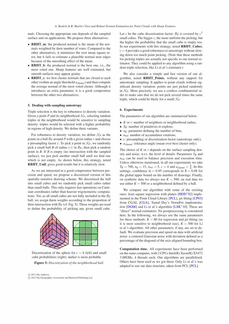
Computation time for a point cloud on sphere with0.2% noise as a function of the number of points.

Figure 6: Computation time (global upper bound only).

Ratio of the execution time with and without the con-fidence interval criterion as a function of noise level.

Figure 7: Impact of the confidence interval criterion.

To illustrate separately the different contributions, we firstdisplay the computation time with the robust global upperbound only (cf. §3), disabling the confidence interval crite-rion. Figure 6 shows the computation time as a function ofthe number of points. The point cloud has been uniformlysampled on a sphere, we added 0.2% noise. As we can see,even with five rotations, the two fast versions of our algo-rithm (RRHT_Cubes and RRHT_Points) are comparable tojet fitting and the Voronoï-based method (NormFet), and arefaster than Li et al.’s algorithm (with the same neighborhoodsize). RRHT_Unif is much slower than existing algorithms,but fully handles anisotropy. The complexity is basically thesame for our methods and for Li et al.’s: it isO(n logn)wheren= |C| is the total number of points in the cloud. Both use aKd-tree for neighborhood search (the logn factor) and repeata similar operation for every vertex (the n factor). However,complexity constants differ much in practice. Note that ourparameter setting here is very demanding on precision as ex-plained below. Figure 6 is thus a kind of worst case scenariofor our method. Much faster computation results are givenlater with only a slightly reduced precision.

TR=700 TR=300nrot=5 nrot=2

w/o with w/o withModel (# vertices) interv. interv. interv. interv.Armadillo (173k) 21 s 20 s 3 s 3 s

Dragon (438k) 55 s 51 s 8 s 7 s

Buddha (543k) 1.1 1 10 s 10 s

Circ. Box (701k) 1.5 1.3 13 s 12 s

Omotondo (998k) 2 1.2 18 s 10 s

Statuette (5M) 11 10 1.5 1.4Room (6.6M) 14 8 2.3 1.6Lucy (14M) 28 17 4 2.5

RRHT_Points algorithm with K = 100 points in theneighborhood, with and without confidence intervals.All times are in minutes unless seconds mentioned.

Table 1: Computation times on real data.

Figure 7 shows the ratio of the execution times with andwithout the confidence interval criterion (cf. §3), for variousnoise levels. (The ratio can be slightly greater than 1 becausetesting the criterion adds a small overhead that is not repaidif not satisfied.) We can see that the criterion significantlyreduces computation. As expected, the impact decreases asnoise level grows because the peaks of the distribution areflatter and separating the highest peak from the second high-est takes longer. The impact also depends on the model. Forcurved and complex shapes, it take more time for a peak toconfidently emerge from the rest of the distribution. Table 1shows computation times of RRHT_Points for several realmodels. As they require less neighbors because they are notnoisy, we use K = 100. For models with a lot of planar sub-surfaces (like the room scan, cf. Figure 2), the addition ofthe confidence interval criteria is very useful.

Precision. We compare the various algorithms with two er-ror measures:

• Root Mean Square (RMS):

RMS =

√

1

|C| ∑P∈C

nP,refnP,est2

• Root Mean Square with threshold (RMS_τ):

RMS_τ =

√

1

|C| ∑P∈C

v2P

where

vP =

{

nP,refnP,est if nP,refnP,est < τπ2 otherwise

nP,ref is the reference (theoretical) normal at P and nP,est theestimated one. RMS is a common measure for precision, butit is not really a rendering measure because it favours smoothreconstruction everywhere, including at edges: a smoothededge is better than having some points with a normal cor-responding to the other side of the edge. That is why we

c© 2012 The Author(s)c© 2012 The Eurographics Association and Blackwell Publishing Ltd.

A. Boulch & R. Marlet / Fast and Robust Normal Estimation for Point Clouds with Sharp Features

From left to right: Jet fitting, Li et al.’s normal estimator, RRHT_Cubes_c and RRHT_Unif_c. Color scale:blue to green is 0 to 10-degree error, red corresponds to an error greater than 10 degrees.

Figure 8: Visual rendering of the precision for three algorithms on a cylinder of 50000 points with 0.2% noise.

Dashed is RRHT_m (mean), dotted is RRHT_b (best),solid is RRHT_c (mean over best cluster).

Figure 9: RMS and RMS_10 for 50k-point closed cylinder.

introduce RMS_τ. This measure considers any angle errorabove threshold τ as very bad (as bad as π

2 ). This penal-izes unwanted smoothing, i.e., equally divergent estimations.Point clouds with normals are better rendered with lowerRMS_τ than lower RMS. In our examples we take τ = 10degrees. Figure 8 is a visual representation of the RMS_10error. Red dots are the badly estimated points. RRHT recon-structs smooth surfaces without grainy effect, but it is not asdiscriminative as Li et al.’s close to the edge.

Robustness to noise. Figure 9 displays precision as a func-tion of noise. Our algorithms are competitive with both mea-

Solid curves represent a fixed nrot for a varying TR,dashed curves represent a fixed TR and varying nrot.

Figure 10: Precision vs speed for a cube with 50k points.

sures, unlike other methods. As expected, RRHT_m givesbetter results for RMS, because of its tendency to smooth,but not for RMS_10. RRHT_c offers the better compromise.Note that Dey’s algorithm is the most efficient for very smallnoise. Fig. 12 illustrates an application to data with realisticnoise. See also Fig. 7 for the impact of noise on running time.

Parameter (in)sensitivity. Figure 10 represents precisionversus computation time, for a fixed nrot or a fixed TR, and anoisy cube. In our experiments, changing the model or noisedoes not affect the curve aspect. Two points are marked,(TR = 700,nrot = 5) and (TR = 300,nrot = 2), which cor-

c© 2012 The Author(s)c© 2012 The Eurographics Association and Blackwell Publishing Ltd.

A. Boulch & R. Marlet / Fast and Robust Normal Estimation for Point Clouds with Sharp Features

From left to right: RRHT_Points_c, RRHT_Cubes_c and RRHT_Unif_c. Color scale: blue to green is 0 to10-degree error, red corresponds to an error greater than 10 degrees. Density is uniform on each face; ifdensity is 1 on right face, then it is 5 for the left face and 10 for the upper face.

Figure 11: Visual rendering of the precision on a corner of 20000 points with density anisotropy.

RRHT_Cubes_c with a radius search corresponding to0.1% of the bounding box diagonal.

Figure 12: Visual rendering of the Château de Sceaux, point

cloud obtained by photogrammetry.

respond to values used in table 1. The first one favors pre-cision; the second one, speed. Other experiments show thattime varies little with c (2–2.5 slower when c varies from 2to 10), nor RMS or RMS_10 (25–30% precision gain). Asfor nφ, it should be large for precision, small for robustness.Experimentally, best nφ values for both RMS and RMS_10are in the range 5–25, with nφ = 15 at most 10% from opti-mum. Time less than doubles when nφ varies from 5 to 25.

Robustness to density anisotropy. Figure 11 shows thenormals computed on a corner sampled with face-specificvariations of density. As expected, no support for anisotropy(RRHT_Points) is very bad whereas uniform ball sampling(RRHT_Unif) recovers well the edges. The cubic discretiza-tion (RRHT_Cubes) compromises well precision vs time (cf.Fig. 6). Figure 13 shows the RMS_10 error for different al-gorithms. As expected, we have a better precision than theother methods, that are not designed to deal with anisotropy.

In the above experiments, neighborhoods are defined witha fixed number of points K. This allows comparison withother algorithms because they use the same notion of neigh-borhood. Also, this data is uniformly sampled (except for theanisotropic corner); a fixed number of points K is thus nearly

Dashed is RRHT_m (mean), dotted is RRHT_b (best),solid is RRHT_c (mean over best cluster).

Figure 13: RMS_10 for a corner with density anisotropy of

20000 points (see Figure 11), function of noise percentage.

the same as a fixed ball of radius r. But variations of densityin real data make neighborhoods with a fixed K inoperative.E.g., the peak of density at the pole of a laser scan can besuch that the actual neighborhood radius r corresponding toa fixed number of points K is on the same order as the noisestandard deviation. It is thus too small to cope with noise.Conversely, data sparsity may also lead to mistakes. E.g.,the leg of a chair in the room (cf. Fig.2) may be sampledwith just a few points and a fixed number of points K willeasily include many points on the floor or on sitting area, asopposed to a fixed neighborhood radius r. For this reason,when operating on real data, we use a neighborhood ball.

Figure 14 shows two dragons with estimated normalswhere the neighborhood radius varies from left to right. Aswe can see on the model without noise, if the radius is greatwe tend to loose small details, but general shape, with sharpfeatures, is maintained. The noisy dragon illustrates the factif the radius is smaller than the noise, it cannot estimate nor-mals, but the results goes better with the increasing radius.

Figure 2 displays parts of a laser scan of a meeting roomwith a few computers. The density of the point cloud de-pends a lot of the incidence. The original point cloud has

c© 2012 The Author(s)c© 2012 The Eurographics Association and Blackwell Publishing Ltd.

A. Boulch & R. Marlet / Fast and Robust Normal Estimation for Point Clouds with Sharp Features

RRHT_Cubes_c with a neighborhood radius rangingfrom a value comparable to the noise standard devia-tion, if any (left), to greater radius values (right).

Figure 14: Normal estimation for the dragon with no added

noise (top) vs 0.2% added noise (bottom).

6.6 millions vertices and with a radius of 0.05 (5 cm at themodel scale), the computation time for RRHT_Cubes is 41min with confidence intervals, as opposed to 48 min with-out, i.e., a 15% improvement. Two details are underlined: acorner with density anisotropy and a beveled edge. Note thatthere is a substantial difference with the time figures in Ta-ble 1. The reason is that searching for 100 neighbors is muchfaster than searching within a given radius, which can corre-spond to thousands of neighbors (or more) when close to thepole. Also, Table 1 uses RRHT_Points, not RRHT_Cubes;not having to pick in the cube is faster.

Robustness to outliers. Our method is robust to a large out-lier ratio. We illustrate that on the Armadillo with both addednoise and outliers (Figure 15). The RMS on the model with0.2% noise is 0.39; adding +100% outliers yields an extra+0.04 on the RMS; adding +300% outliers yields +0.15 onthe RMS. When the contamination ratio increases, the firstpoints not well estimated are the sharp points, whose nor-mal distribution is flatter than the distribution on a regularsurface: they are more sensitive to noise and outliers.

Armadillo with 0.2% noise and +100% outliers (top),+300% (bottom). Neighborhood radius r is 3% ofbounding box diagonal. Outliers are uniformly drawnat distance at most r from original point set. Outliersare dropped in result for visual rending (right).

Figure 15: Outlier robustness of RRHT on Armadillo.

7. Conclusion

We have proposed a novel method for estimating normals forpoint clouds that preserves sharp features and that is robustto noise and outliers. Different variants or parameter settingsoffer good compromises between precision and computationtime. We have shown that our method is at least as preciseand noise-resistant as state-of-the-art methods that preservesharp features, while being almost an order of magnitudefaster. It can also handle anisotropy with minor speed andprecision losses. Besides, it is simple and easy to program.

As future work, it would be interesting to improve speedwith an adaptive choice of variants and parameters, and thetime saved could in turn be traded against more precision.The idea would be to use cubic drawing by default but tolocally switch to the uniform drawing scheme where estima-tion is known to be inaccurate. Also, an adaptive neighbor-hood would help reducing the number of parameters. More-over, some kinds of laser scans organize data; preliminaryexperiments show that making a good use this organizationgreatly reduces computation time.

Acknowledgments

We are grateful to Pierre Alliez for helpful advices. Thanksto Bao Li and Tamal Dey for providing the code used forcomparison. Armadillo, Lucy, Dragon, Buddha, and Stat-uette point clouds come from the Stanford 3D ScanningRepository; Circular Box and Omotondo from Aim@Shape.

c© 2012 The Author(s)c© 2012 The Eurographics Association and Blackwell Publishing Ltd.

A. Boulch & R. Marlet / Fast and Robust Normal Estimation for Point Clouds with Sharp Features

References

[ABCO∗01] ALEXA M., BEHR J., COHEN-OR D., FLEISHMAN

S., LEVIN D., SILVA C. T.: Point set surfaces. In IEEE Visual-

ization (October 2001), IEEE Comp. Soc., pp. 21–28. 1

[ACSTD07] ALLIEZ P., COHEN-STEINER D., TONG Y., DES-BRUN M.: Voronoi-based variational reconstruction of unori-ented point sets. In Proceedings of the Fifth Eurographics Sympo-sium on Geometry Processing, Barcelona, Spain, July 4-6, 2007

(2007), Belyaev A. G., Garland M., (Eds.), vol. 257 of ACM In-

ternational Conference Proceeding Series, Eurographics Associ-ation, pp. 39–48. 2

[Bal87] BALLARD D. H.: Generalizing the hough transform todetect arbitrary shapes. In RCV87 (1987), pp. 714–725. 2

[BELN11] BORRMANN D., ELSEBERG J., LINGEMANN K.,NÜCHTER A.: The 3D Hough Transform for plane detection inpoint clouds: A review and a new accumulator design. 3D Res.

2, 2 (Mar. 2011), 32:1–32:13. 4

[BLK10] BARINOVA O., LEMPITSKY V. S., KOHLI P.: On de-tection of multiple object instances using Hough transforms. InCVPR (2010), IEEE, pp. 2233–2240. 2

[CGA] CGAL, Computational Geometry Algorithms Library.http://www.cgal.org. 5

[CLP10] CHAUVE A.-L., LABATUT P., PONS J.-P.: Robustpiecewise-planar 3D reconstruction and completion from large-scale unstructured point data. In CVPR (2010), IEEE, pp. 1261–1268. 1

[CP03] CAZALS F., POUGET M.: Estimating differential quanti-ties using polynomial fitting of osculating jets. In Proceedings ofthe 2003 Eurographics/ACM SIGGRAPH symposium on Geome-

try processing (2003), SGP ’03, pp. 177–187. 1, 5

[Dav88] DAVIES E. R.: Application of the generalized Houghtransformation to corner detection. Computers and Digital Tech-niques, IEEE proceedings 15, 1 (1988), 49–54. 2

[DG06] DEY T. K., GOSWAMI S.: Provable surface reconstruc-tion from noisy samples. Comput. Geom. 35, 1-2 (2006), 124–141. 1, 5

[DH72] DUDA R., HART P. E.: Use of the Hough transformationto detect lines and curves in pictures. CACM 15 (1972), 11–15.2

[GG07] GUENNEBAUD G., GROSS M. H.: Algebraic point setsurfaces. ACM Trans. Graph 26, 3 (2007), 23. 1

[GL09] GALL J., LEMPITSKY V.: Class-specific hough forestsfor object detection. In CVPR (2009), pp. 1022–1029. 2

[HDD∗92] HOPPE H., DEROSE T., DUCHAMP T., MCDONALD

J., STUETZLE W.: Surface reconstruction from unorganizedpoints. SIGGRAPH Comput. Graph. 26, 2 (July 1992), 71–78.1, 2, 5

[HLZ∗09] HUANG H., LI D., ZHANG H., ASCHER U., COHEN-OR D.: Consolidation of unorganized point clouds for surfacereconstruction. ACM Trans. Graph. 28, 5 (Dec. 2009), 176:1–176:7. 1

[Hoe63] HOEFFDING W.: Probability inequalities for sums ofbounded random variables. Journal of the American Statistical

Association 58, 301 (March 1963), 13–30. 3

[Hou62] HOUGH P. V. C.: Method and means for recognizingcomplex patterns. U.S. Patent 3.069.654 (1962). 2

[IK88] ILLINGWORTH J., KITTLER J. V.: A survey of the Houghtransform. CVGIP: Image Understanding 44, 1 (Oct. 1988), 87–116. 2

[JDZ04] JONES T. R., DURAND F., ZWICKER M.: Normal im-provement for point rendering. IEEE Computer Graphics and

Applications 24, 4 (2004), 53–56. 1

[KEB91] KIRYATI, ELDAR, BRUCKSTEIN: A probabilisticHough transform. PATREC: Pattern Recognition, Pergamon

Press 24 (1991). 2

[KPW∗10] KNOPP J., PRASAD M., WILLEMS G., TIMOFTE R.,GOOL L. J. V.: Hough transform and 3D SURF for robustthree dimensional classification. In 11th European Conference onComputer Vision (ECCV 2010), Proc., Part VI (2010), vol. 6316of LNCS, Springer, pp. 589–602. 2

[Low04] LOWE D. G.: Distinctive image features from scale-invariant keypoints. International Journal of Computer Vision

60, 2 (2004), 91–110. 2

[LSK∗10] LI B., SCHNABEL R., KLEIN R., CHENG Z.-Q.,DANG G., JIN S.: Robust normal estimation for point cloudswith sharp features. Computers & Graphics 34, 2 (2010), 94–106. 2, 5

[MdGD∗10] MULLEN P., DE GOES F., DESBRUN M., COHEN-STEINER D., ALLIEZ P.: Signing the unsigned: Robust surfacereconstruction from raw pointsets. Comput. Graph. Forum 29, 5(2010), 1733–1741. 2

[MNG04] MITRA N. J., NGUYEN A., GUIBAS L.: Estimatingsurface normals in noisy point cloud data. In special issue of

International Journal of Computational Geometry and Applica-

tions (2004), vol. 14, pp. 261–276. 1

[ÖGG09] ÖZTIRELI A. C., GUENNEBAUD G., GROSS M. H.:Feature preserving point set surfaces based on non-linear kernelregression. Comput. Graph. Forum 28, 2 (2009), 493–501. 1

[Oka09] OKADA R.: Discriminative generalized Hough trans-form for object dectection. In ICCV (2009), IEEE, pp. 2000–2005. 2

[PCL] PCL, Point Cloud Library. http://pointclouds.org. 5

[PKKG03] PAULY M., KEISER R., KOBBELT L. P., GROSS M.:Shape modeling with point-sampled geometry. ACM Trans.

Graph. 22, 3 (July 2003), 641–650. 1

[PWP∗11] PHAM M.-T., WOODFORD O. J., PERBET F., MAKI

A., STENGER B., CIPOLLA R.: A new distance for scale-invariant 3D shape recognition and registration. In IEEE Interna-

tional Conference on Computer Vision, ICCV 2011, Barcelona,

Spain, November 6-13, 2011 (2011), IEEE, pp. 145–152. 2

[RL00] RUSINKIEWICZ S., LEVOY M.: QSplat: A multireso-lution point rendering system for large meshes. In Proc. of

the Computer Graphics Conference (SIGGRAPH) (2000), ACMPress, pp. 343–352. 1

[SWK07] SCHNABEL R., WAHL R., KLEIN R.: EfficientRANSAC for point-cloud shape detection. Computer Graphics

Forum 26, 2 (June 2007), 214–226. 1

[TM78] TSUJI S., MATSUMOTO F.: Detection of ellipses by amodified Hough transformation. IEEE Transactions on Comput-

ers 27 (1978), 777–781. 2

[XO93] XU L., OJA E.: Randomized Hough Transform (RHT):Basic mechanisms, algorithms, and computational complexities.CVGIP: Image Understanding 57, 2 (Mar. 1993), 131–154. 2

[XOK90] XU L., OJA E., KULTANEN P.: A new curve detectionmethod: Randomized Hough Transform (RHT). Pattern Recog-

nition Letters 11, 5 (May 1990), 331–338. 2

[YLL∗07] YOON M., LEE Y., LEE S., IVRISSIMTZIS I., SEIDEL

H.-P.: Surface and normal ensembles for surface reconstruction.Comput. Aided Des. 39, 5 (May 2007), 408–420. 1

c© 2012 The Author(s)c© 2012 The Eurographics Association and Blackwell Publishing Ltd.