Fast and accurate irradiance calculations for … 6, 10625–10662, 2009 Irradiance calculations C....

BGD6, 10625–10662, 2009

Irradiancecalculations

C. D. Mobley et al.

Title Page

Abstract Introduction

Conclusions References

Tables Figures

J I

J I

Back Close

Full Screen / Esc

Printer-friendly Version

Interactive Discussion

Biogeosciences Discuss., 6, 10625–10662, 2009www.biogeosciences-discuss.net/6/10625/2009/© Author(s) 2009. This work is distributed underthe Creative Commons Attribution 3.0 License.

BiogeosciencesDiscussions

This discussion paper is/has been under review for the journal Biogeosciences (BG).Please refer to the corresponding final paper in BG if available.

Fast and accurate irradiance calculationsfor ecosystem modelsC. D. Mobley1, L. K. Sundman2, W. P. Bissett3, and B. Cahill4

1Sequoia Scientific, Inc., 2700 Richards Road, Suite 107, Bellevue, WA 98005, USA2Sundman Consulting, 1453 S. Haleyville Circle, Aurora, CO 80018, USA3WeoGeo, 2828 SW Corbett Ave., Suite 135, Portland, OR 97201, USA4Institute of Marine and Coastal Science, Rutgers University, 71 Dudley Road,New Brunswick, NJ 08901, USA

Received: 7 October 2009 – Accepted: 28 October 2009 – Published: 16 November 2009

Correspondence to: C. D. Mobley ([email protected])

Published by Copernicus Publications on behalf of the European Geosciences Union.

10625

http://www.biogeosciences-discuss.net

http://www.biogeosciences-discuss.net/6/10625/2009/bgd-6-10625-2009-print.pdf

http://www.biogeosciences-discuss.net/6/10625/2009/bgd-6-10625-2009-discussion.html

http://creativecommons.org/licenses/by/3.0/

BGD6, 10625–10662, 2009


C. D. Mobley et al.

Title Page



Tables Figures

J I

J I

Back Close

Full Screen / Esc



Abstract

Coupled physical-biological-optical ocean ecosystem models often use sophisticatedtreatments of their physical and biological components, while oversimplifying the opti-cal component to the possible detriment of the ecosystem predictions. To bring opticalcomputations up to the standard required by recent ecosystem models, we developed5

a computationally fast numerical model, named EcoLight, that solves the azimuthallyaveraged radiative transfer equation to obtain accurate in-water spectral irradiancesfor use in calculations of photosynthesis and photo-oxidation. To evaluate its computa-tional features, we incorporated EcoLight into an idealized physical-biological model foropen-ocean Case 1 waters and compared ten-year simulations for a simple analytical10

irradiance model vs. EcoLight numerical calculations. After optimization, the EcoLightrun times are less than 30% more than for the analytical irradiance model. Moreover,EcoLight is suitable for use in Case 2 and optically shallow waters, for which no ana-lytical irradiance models exist. EcoLight also computes ancillary quantities such as theremote-sensing reflectance, which can be useful for ecosystem validation.15

1 Introduction

The fundamental measure of light energy in an aquatic system is the spectral radi-ance L, which in horizontally homogeneous water bodies is a function of time, depth,direction, and wavelength. In situations relevant to ecosystem modeling, changes inthe water absorption and scattering properties and boundary conditions occur on time20

scales much longer than needed for the radiance to achieve steady state, and the timedependence can be omitted when solving the radiative transfer equation (RTE). Theradiance at any particular time is then L(z,θ,φ,λ), where z is depth, measured positivedownward from z= 0 at the mean water surface; θ is the polar angle, with θ= 0 refer-ring to light traveling toward the nadir (+z) direction; φ is the azimuthal direction; and25

λ is the wavelength. (This paper uses the notation and terminology of Mobley, 1994.)

10626





BGD6, 10625–10662, 2009


C. D. Mobley et al.

Title Page



Tables Figures

J I

J I

Back Close

Full Screen / Esc



The directional information contained in the radiance is usually irrelevant becausewater constituents such as phytoplankton and dissolved substances are assumedequally likely to interact with a photon regardless of its direction of travel. Therefore,the spectral scalar irradiance,

Eo(z,λ)=∫ 2π

0

∫ π

0L(z,θ,φ,λ)sinθdθdφ, (1)5

is the fundamental radiometric quantity necessary for predictions of aquatic primaryproductivity, photochemical reactions, and heating of water. When modeling photosyn-thesis, which depends on the number of photons absorbed, it is necessary to multi-ply Eo(z,λ) by λ/hc, where h is Planck’s constant and c is the speed of light. Thisconverts the energy units of the spectral irradiance, Wm−2nm−1, to quantum units,10

photonss−1m−2nm−1.A simple measure of the total light available for photosynthesis, the photosyntheti-

cally available radiation (PAR),

PAR(z)=∫ 700

400Eo(z,λ)

λhc

dλ, (2)

is frequently used in ecosystem models. Some models approximate PAR in terms of15

the downwelling irradiance Ed . However, the use of Ed instead of Eo in Eq. (2) signifi-cantly underestimates PAR (Sakshaug et al., 1997), especially near the surface and inshallow water where upwelling light can significantly contribute to the total irradiance.

Simple analytical models are commonly employed for estimating the dependence ofPAR on time (diurnal, inter-day, or seasonal changes), depth, and water inherent optical20

properties (IOPs, namely the water absorption and scattering properties). Climatolog-ical data are often used to provide the time dependence of the (downwelling) surfaceirradiance. If intraday variability of the light field is included, it is sometimes expressedby a sinusoidal (Bissett et al., 1994) or sawtooth (Evans and Parslow, 1985) function.

10627





BGD6, 10625–10662, 2009


C. D. Mobley et al.

Title Page



Tables Figures

J I

J I

Back Close

Full Screen / Esc



Some studies have used astronomical models to estimate the solar radiation as a func-tion of time (Fasham, 1995; Hurtt and Armstrong, 1996), while others neglected thediurnal variation of light completely, using climatological daily-averaged values (Oguzet al., 1996). Errors associated with approximating (or neglecting) temporal variabilityare greatest when photo-limited and photo-adaptive effects are significant.5

Traditionally, coupled ecosystem models have incorporated simple analytical formu-las to predict PAR(z) from a given chlorophyll profile and from an estimate of PAR atthe sea surface (Evans and Parslow, 1985; Fasham et al., 1990; Doney et al., 1996;Hurtt and Armstrong, 1996; Oschlies and Garcon, 1998). Although these analyticalPAR models are computationally fast, they can produce estimates that differ by a factor10

of three near the sea surface and by a factor of ten at the bottom of the euphotic zone(Zielinski et al., 1998). Indeed, the depth of the euphotic zone, if defined as the depthwhere PAR decreases to one percent of its surface value, differs by almost a factorof two among these models. Errors of this magnitude are unacceptable for quantita-tive predictions of primary productivity or upper-ocean thermal structure. Additional15

inaccuracies can be found in the application of the PAR formulas, such as the use ofdownwelling plane irradiance Ed as a proxy for the scalar irradiance.

The depth dependence of the irradiance is often expressed as a simple exponentialdecay function, PAR(z)=PAR(0)exp(−KPARz), where KPAR is an attenuation coefficientfor PAR. Kyewalyanga et al. (1992) accounted for the different path lengths associated20

with direct solar and diffuse light by defining two attenuation coefficients that dependon the mean cosine of the downwelling radiance and on the solar elevation. Somemodels (Fasham, 1995; Hurtt and Armstrong, 1996; Oguz et al., 1996; Moore et al.,2002) consider the contributions to the attenuation by different components (pure water,chlorophyll, CDOM, etc.), but still neglect the spectral dependence of the attenuation25

of light. Most assume that the attenuation rates of each component are constant withdepth (Evans and Parslow, 1985; Fasham, 1995; Hurtt and Armstrong, 1996; Oguzet al., 1996; Kyewalyanga et al., 1992). Others use depth-averaged values (Doneyet al., 1996). Moore et al. (2002) use a depth-averaged PAR value within the mixed

10628





BGD6, 10625–10662, 2009


C. D. Mobley et al.

Title Page



Tables Figures

J I

J I

Back Close

Full Screen / Esc



layer. Such simplifications can induce significant errors, especially near the surfacewhere the spectral distribution of the light field is changing rapidly with depth as thewater preferentially absorbs some wavelengths while transmitting others. Errors gen-erated near the surface propagate with depth and thereby influence on the light fieldthroughout the euphotic zone.5

Many papers set the PAR value just below the surface to be 45–52% of the total solarillumination, citing Baker and Frouin (1987). However, Baker and Frouin reported ratiosof the downwelling plane irradiance in the 400–700 nm range just above the surface tothe total solar illumination (plane irradiance) at the top of the atmosphere. Their workstudied the sensitivity of this ratio to atmospheric conditions. They did not consider10

scalar irradiances or PAR and they did not study the transmittance of the light throughthe sea surface.

Simpson and Dickey (1981) investigated the sensitivity of the total downwelling irra-diance over the entire spectrum as estimated from five models to a number of factors.They divided the models into categories based on the mathematical form of the mod-15

els: simple exponential, bimodal, arctangent, and multiband. Zielinski et al. (1998)also used these categories to evaluate the influence of PAR models by applying themto a set of ESTOC (European Station for Time-series in the Ocean Canary Islands;located at 29◦10′ N, 15◦30′ W) data and a one-dimensional (depth dependent) bio-physical model. They quantified the effect of the variation between the different PAR20

models. However, conclusions about the influence of PAR on their coupled model weresomewhat limited by the absence of measurements of the actual PAR.

Although simple PAR models are computationally convenient, any ecosystem modelbased on PAR is limited in its realism, regardless of how accurately PAR is computed.Different species of phytoplankton have different pigment suites, which respond differ-25

ently to different wavelengths. Therefore, any model that attempts to describe competi-tion between different species or functional groups having different pigments must usespectral irradiance, not a wavelength-integrated measure of the light.

The Ecosystem Simulation (EcoSim) model of Bissett et al. (1999a,b) moves beyond

10629





BGD6, 10625–10662, 2009


C. D. Mobley et al.

Title Page



Tables Figures

J I

J I

Back Close

Full Screen / Esc



PAR calculations and calculates and uses the spectral distribution of light. EcoSim in-cludes four phytoplankton functional groups, each with a characteristic pigment suitethat changes over time with light and nutrient conditions. To model light effects onchanges within and competition between these groups, EcoSim uses an approximatemodel for the spectral scalar irradiance in Case 1 waters (described below). The spec-5

tral irradiance is used with the modeled pigment suites to create competition amongphytoplankton groups based on their photosynthetic action spectra. In addition to deal-ing explicitly with spectral light and its impacts on phytoplankton community structure,EcoSim also explicitly models the feedbacks from changes in IOPs, e.g. CDOM pho-tolysis and photoacclimation of phytoplankton, which in turn drive changes in the color10

and intensity of light at depth. Although the EcoSim spectral irradiance model is suffi-ciently fast for use in coupled physical-biological ecosystem simulations involving manygrid points and time steps, it does rest on several approximations that can limit its ac-curacy even in Case 1 waters, and it is not applicable to Case 2 or optically shallowwaters.15

There is today much interest in the modeling of coastal waters, which are oftenCase 2 due to resuspended sediments or terrigenous particles and dissolved sub-stances, and which may be shallow enough for bottom reflectance to make a significantcontribution to the scalar irradiance. If EcoSim or similar models are to accurately sim-ulate such optically complex waters, they must incorporate spectral irradiance models20

that are computationally fast, accurate, and applicable to any water body. To addressthis need, we have developed a specialized version of the HydroLight radiative trans-fer model (Mobley et al., 1993; Mobley, 1994, and http://www.hydrolight.info), calledEcoLight, which is designed to bring the optical component of ecosystem models upto the level of sophistication found in the latest physical and biological models. Fujii25

et al. (2007) incorporated an early version of EcoLight into a physical-biological modeland showed that improved optical calculations help constrain ecosystem behavior andgave predictions consistent with observations in simulations of an equatorial Pacific up-welling region. They however did not consider ways of optimizing the EcoLight calcula-

10630





http://www.hydrolight.info

BGD6, 10625–10662, 2009


C. D. Mobley et al.

Title Page



Tables Figures

J I

J I

Back Close

Full Screen / Esc



tions to preserve accuracy while minimizing run times, nor did they compare long-termecosystem behavior for simple vs. accurate light calculations.

We incorporated EcoLight into a coupled model and compared its performance withthe spectral irradiance model used in EcoSim. We first briefly describe the physicaland biological models, and then EcoLight and the coupled model. We then compare5

the predictions made for an idealized ecosystem simulation when using the originalEcoSim light model with those made using various EcoLight options.

2 The ecosystem model

Our ecosystem model has separate submodels for the physical, biological, and opticalcomponents, which we describe next.10

2.1 The ROMS physical model

The physical model used here is the Regional Ocean Modeling System (ROMS).ROMS is widely used for coastal and shelf circulation and coupled physical-biologicalapplications (e.g. Dinniman et al., 2003; Lutjeharms et al., 2003; Marchesiello etal., 2003; Peliz et al., 2003; Fennel et al., 2006, 2008; Fennel and Wilkin, 2009;15

Wilkin, 2006; Cahill et al., 2008). The ROMS computational kernel (Shchepetkin andMcWilliams, 1998, 2003, 2005) produces accurate evolution of tracer fields, which is aparticularly attractive feature for biogeochemical modeling because it facilitates accu-rate interaction among tracers and accounting of total nutrient and carbon budgets.

The present study uses a 6×6 horizontal grid domain with periodic lateral boundary20

conditions. This spatially limited domain was chosen to minimize run times during theEcoLight code development and evaluation simulations. For the simulations presentedbelow, the grid is centered off the continental shelf of the eastern United States near73.2◦ W and 38.8◦ N, as shown in Fig. 1. The horizontal grid resolution is approximately10 km. The vertical grid has 30 points covering the upper 210 m of the water column;25

10631





BGD6, 10625–10662, 2009


C. D. Mobley et al.

Title Page



Tables Figures

J I

J I

Back Close

Full Screen / Esc



the vertical resolution ranges from approximately 2 m near the sea surface to 15 m atdepth.

In our simulations the ROMS model was driven by an annual cycle of external ir-radiances and winds obtained from reanalysis of gridded atmospheric data at 6-hourresolution obtained from the European Centre for Medium-Range Weather Forecasts.5

Water column heating as needed to compute mixed layer dynamics in ROMS is ob-tained from simple analytical models for band-integrated short and long-wave radiation.Figure 2 shows the daily local-noon short-wave irradiances used as inputs to ROMS.This same annual cycle was repeated for each simulation year.

2.2 The EcoSim biological model10

EcoSim is an ecological-optical modeling system that was developed for simulationsof carbon cycling and biological productivity (Bissett et al., 1999a,b, 2005, 2008). Itincludes four phytoplankton functional groups (FG1 is small diatoms, FG2 is large di-atoms, FG3 is large dinoflagellates, and FG4 is synechococcus), each with a charac-teristic pigment suite that varies with the group carbon-to-chlorophyll a ratio, C:Chla.15

EcoSim spectrally-resolves the irradiance as opposed to using wavelength-integratedirradiance. This allows differential growth of different phytoplankton groups that haveunique pigment suites. The properties of each functional group evolve over time asa function of light and nutrient conditions. Other EcoSim components include bac-teria, dissolved organic matter, dissolved inorganic carbon cycling and 5 nutrients20

(NO3,NH4,PO4,SiO, and FeO). The interactions between EcoSim’s components de-scribe autotrophic growth of and competition between the four phytoplankton groups,differential carbon and nitrogen cycling, nitrogen fixation, and grazing. The maximumphytoplankton growth is modulated by temperature (Eppley, 1972). Loss is effected bygrazing and excretion. Grazing accounts for the majority of the biomass sink in this25

model and is considered the closure term of the phytoplankton equations (Steele andHenderson, 1992). Grazing is modeled as a Michaelis-Menten function based on thefunctional groups’ biomass (Bissett et al., 1999a). The initial application of EcoSim

10632





BGD6, 10625–10662, 2009


C. D. Mobley et al.

Title Page



Tables Figures

J I

J I

Back Close

Full Screen / Esc



to predictions of seasonal cycles of carbon cycling and phytoplankton dynamics in theSargasso Sea showed that its predictions were consistent with measurement of variousbiological and chemical quantities at the Bermuda Atlantic Time-series Study (BATS)station (Bissett et al., 1999a).

EcoSim version 2.0 as used in the present simulations includes nutrient recycling to5

replenish nutrients lost as particles sink below the bottom of the maximum simulationdepth. Fecal material and phytoplankton sink at various rates: 0.01 mday−1 for FG1,0.1 mday−1 for FG2, 10 mday−1 for fecal material, and no sinking for FG3, FG4 anddissolved components. When particles reach the maximum depth, their masses areconverted to nutrients as follows: fecal and phytoplankton carbon are converted to10

dissolved inorganic carbon, fecal and phytoplankton nitrogen are converted to NO3,phosphorous is converted to PO4, silicon to SiO, and iron to FeO. The flux of nutrientsout of the bottom of the model domain is immediately converted into a correspondinginflux of nutrients into the bottom of the model domain. Other modifications to EcoSimsince its original publication are described in Bissett et al. (2004).15

The absorption spectra of the phytoplankton functional groups change with light andnutrient adaptation. The four groups therefore respond differently to various wave-lengths of the available light, and each group responds differently over time. EcoSimrequires spectral irradiances at 5 nm bandwidths between 400 and 700 nm in orderto model the changes within each functional group and competition between them.20

The use of spectral irradiance rather than broadband PAR in modeling phytoplanktondynamics is a distinguishing feature of EcoSim. The standard EcoSim code, whichwe call the analytic light (AL) version, first calls the RADTRAN (Gregg and Carder,1990) atmospheric radiative transfer model to obtain the spectral downwelling directand diffuse plane irradiances just beneath the sea surface for clear sky conditions.25

These clear-sky irradiances are functions of the atmospheric conditions (aerosol type,humidity, etc.) and solar zenith angle. The model can be driven by measured or cli-matological sea surface PAR measurements. When this is done, PAR computed fromthe RADTRAN spectrum is compared with the measured PAR, and the PAR ratio is

10633





BGD6, 10625–10662, 2009


C. D. Mobley et al.

Title Page



Tables Figures

J I

J I

Back Close

Full Screen / Esc



used to rescale the computed spectral irradiances at the sea surface. In the presentsimulations, the wavelength-integrated RADTRAN irradiances are rescaled to give thecurrent value of the ROMS short-wave irradiance as shown in Fig. 2.

The RADTRAN-computed and rescaled spectral downwelling plane irradiances justbeneath the sea surface are then propagated to depth using5

Ed (z,λ)=Ed (0,λ)exp[−∫ z

0Kd (z′,λ)dz′

](3)

and a simple model for Kd ,

Kd (z,λ)=a(z,λ)+bb(z,λ)

µd (z,λ). (4)

Here a(z,λ) is the total absorption coefficient (the sum of absorption by pure water andthe various particulate and dissolved components), and bb(z,λ) is the total backscatter10

coefficient. The phytoplankton absorption is obtained from the concentrations of thefunctional groups and their chlorophyll-specific absorption spectra. The backscattercoefficient is obtained from the chlorophyll-dependent model of Morel and Maritorena(2001) for Case 1 waters, using the total Chla concentration. The total scattering co-efficient b(z,λ) is obtained from the Case 1 model of Gordon and Morel (1983). The15

mean cosine for downwelling irradiance, µd (z,λ), is itself modeled by a simple functionthat merges estimates of the near-surface and asymptotic-depth mean cosines (Bissettet al., 1999b, Eqs. 18–22). The value of µd at the surface is set to the cosine of thein-water solar zenith angle; the value at the maximum depth is set to 0.75, which is atypical value for oceanic asymptotic light fields. Finally, the needed scalar irradiance20

Eo(z,λ) is obtained from the computed Ed (z,λ) and the approximation

Eo(z,λ)≈Ed (z,λ)Kd (z,λ)

a(z,λ). (5)

10634





BGD6, 10625–10662, 2009


C. D. Mobley et al.

Title Page



Tables Figures

J I

J I

Back Close

Full Screen / Esc



EcoSim AL uses Eqs. (3–5) to compute the irradiance to a depth at which Ed (z,λ)integrated from 400 to 700 nm becomes less than 1Wm−2.

In the 6×6 grid ROMS-EcoSim code, the outer layer of grid points seen in Fig. 1 isused to impose the periodic boundary conditions. Therefore the EcoSim code com-putes the biology only at the interior 4×4 block of grid points. The biology is updated5

at each ROMS time step and interior grid point using the analytic formulas for thescalar irradiance just described. However, the irradiances computed within EcoSim donot feed back to the ROMS code which, for programming simplicity when merging thecodes, retains its original short and long-wave light parameterization for mixed-layerheating calculations. Thus the physical model influences the biology via temperature10

and mixing, but the optical model employed within EcoSim does not influence the phys-ical model. This simplification was retained in the present study to avoid alterations tothe ROMS code.

2.3 The EcoLight radiative transfer model

Accurate predictions of primary production require accurate predictions of the ambient15

spectral scalar irradiance. Numerical models that solve the scalar RTE are currentlyavailable (Mobley et al., 1993) and can provide highly accurate predictions of the lightfield, in particular the scalar irradiance as a function of depth and wavelength. How-ever, the computational times required by these numerical models are far too great fortheir inclusion in large coupled models that need irradiance predictions at many spatial20

locations and times of day.The HydroLight radiative transfer model (Mobley et al., 1993; Mobley, 1994, and

www.hydrolight.info) provides an accurate solution of the scalar RTE for any waterbody, given the inherent optical properties of the water body, the incident sky radiance,and the bottom reflectance (in finite-depth waters). Although the standard version of25

HydroLight is computationally very efficient, its run times are still much too long for usein ecosystem models. HydroLight computes the radiance for a set of M polar direc-tions and N azimuthal directions. The total number of directions is then (M−2)N+2;

10635





www.hydrolight.info

BGD6, 10625–10662, 2009


C. D. Mobley et al.

Title Page



Tables Figures

J I

J I

Back Close

Full Screen / Esc



namely N azimuthal angles for each non-polar-cap direction, plus the zenith and nadirpolar cap directions. The computational time is proportional to this number of directionssquared, because each direction interacts via scattering with every other direction. Alarge part of the HydroLight run time is used to compute the azimuthal dependence ofthe radiance distribution. A slightly optimized version of HydroLight 3.1 was developed5

by Liu et al. (1999). Liu et al. (2002) developed a multi-parameter look-up-table forscalar irradiance in homogeneous waters. Their model is based on HydroLight simu-lations and gives PAR profiles that are within a few percent of HydroLight values butruns four orders of magnitude faster. However, the Liu et al. (2002) model is not suitedto the needs of EcoSim when modeling inhomogeneous or Case 2 waters.10

Ecosystem models require only the scalar irradiance Eo as a function of depth andwavelength, which is computed from an azimuthal integration of the radiance as seenin Eq. (1). The azimuthal dependence of the radiance, obtained at great computationalexpense in HydroLight, is thus lost in the integration of Eq. (1). This means that theRTE can be azimuthally averaged to obtain an equation for the azimuthally averaged15

radiance as a function of polar angle. The numerical solution of the resulting RTE ismuch simpler than in HydroLight. In particular, there is no azimuthal decomposition ofthe radiance into Fourier amplitudes. Only M azimuthally averaged radiances need becomputed, and the run time is proportional to M2. The standard version of HydroLightuses M = 20 θ directions and N = 24 φ directions, which gives 10 degree resolution20

in the polar angle (including two polar caps with 5 degree half-angles) and 15 degreeresolution in the azimuthal angle. Eliminating the azimuthal dependence from the cal-culations therefore gives approximately a factor-of-400 reduction in the computationtime (allowing for certain calculations that are independent of angular resolution).

Based upon this observation, we developed a highly optimized version of Hydro-25

Light 4.2, called EcoLight, which solves the azimuthally averaged RTE as a function ofdepth and wavelength for any water body. EcoLight requires the same IOP and bound-ary condition inputs as HydroLight, and the resulting irradiances are computed with thesame accuracy as HydroLight. Related quantities such as the irradiance reflectance,

10636





BGD6, 10625–10662, 2009


C. D. Mobley et al.

Title Page



Tables Figures

J I

J I

Back Close

Full Screen / Esc



nadir-viewing water-leaving radiance and remote-sensing reflectance, and diffuse at-tenuation coefficients also computed by EcoLight. Although those ancillary quantitiesare not needed as inputs to most ecosystem models, they can be of use in ecosys-tem model validation. In particular, the water-leaving radiance and remote-sensing re-flectance allow ecosystem validation using satellite radiometric measurements without5

the intervening step of converting radiometric measurements into chlorophyll concen-trations via imperfect chlorophyll algorithms. Quantities such as the remote-sensingreflectance are not available from the simple analytic light models.

Various additional optimizations to the EcoLight code were made. The most impor-tant are the use of a piecewise homogeneous water column, solution of the RTE to10

different depths at different wavelengths, and wavelength skipping.The ROMS-EcoSim code models the water column as a stack of homogeneous lay-

ers of variable thickness. Therefore the IOPs within a given water layer are indepen-dent of depth. The EcoLight code takes advantage of the depth independence of theIOPs within a layer to reduce the computation needed to solve the RTE for the depth15

dependence of the irradiances within each layer.HydroLight solves the RTE to a user-specified geometric depth, which is the same for

every wavelength and must be chosen before the run is started. This becomes compu-tationally expensive at wavelengths where the IOPs are large (e.g., at red wavelengthsowing to pure water absorption or at blue wavelengths owing to CDOM absorption) cor-20

responding to a large optical depth for a given geometric depth. EcoSim requires thespectral scalar irradiance only to the bottom of the euphotic zone, below which it doesnot perform primary production calculations. Therefore, it is necessary to compute theirradiance only to that depth, which varies with the biological state of the ocean andcannot be predetermined.25

In EcoLight the goal is to solve the RTE to the shallowest depth possible and then toextrapolate the scalar irradiance to greater depths. To determine the depth to which theRTE is to be solved at a particular wavelength, an equation of the form of Eq. (3) canbe written using Eo instead of Ed and Ko instead of Kd . Note that Ko is an apparent

10637





BGD6, 10625–10662, 2009


C. D. Mobley et al.

Title Page



Tables Figures

J I

J I

Back Close

Full Screen / Esc



optical property and is not known until the RTE has been solved. However, exceptvery near the sea surface where boundary effects are important, Ko is roughly equalto Kd , the diffuse attenuation coefficient for downwelling plane irradiance (Ko becomesexactly equal to Kd at great depths in homogeneous water). To first order (e.g., Mobley,1994, Eq. 5.65) Kd ≈ a/µd , where a is the absorption coefficient and µd is the mean5

cosine of the downwelling radiance distribution. In typical waters, µd ≈ 3/4. Thus, inthe modified Eq. (3) we can approximate Ko(z,λ) by the absorption coefficient a(z,λ)and define

Fo ≡Eo(zo,λ)

Eo(0,λ)≈exp

[−∫ zo

0a(z′,λ)dz′

]. (6)

Given the absorption coefficient, which is known before the RTE is solved, this equation10

can be used to estimate the depth zo at which the scalar irradiance will decrease to afraction Fo of its surface value. Because of the approximations used, the estimated zowill always be greater than the actual zo.

At the first wavelength, zo is obtained from Eq. (6) for a pre-specified Fo, and thebottom boundary condition is then applied at this depth. At the first wavelength, λ1,15

the RTE is solved to the estimated depth, zo(est;λ1), determined as just described.After the RTE is solved, the actual depth zo(exact;λ1) at which Eo(z,λ1) decreasedto FoEo(0,λ1) can be determined. At subsequent wavelengths, the ratio of actual toestimated zo values from the previous wavelength is used to correct the initial estimateat the present wavelength:20

zo(final;λj )= zo(est;λj )zo(exact;λj−1)

zo(est;λj−1). (7)

Thus, if the initial absorption-based estimate of zo at the previous wavelength was20% too large, it is assumed that the initial estimate at the current wavelength is also20% too large, and the initial estimate of zo is reduced accordingly. This adjustment,which is based upon the exact depth at the previous wavelength, corrects for the error25

10638





BGD6, 10625–10662, 2009


C. D. Mobley et al.

Title Page



Tables Figures

J I

J I

Back Close

Full Screen / Esc



inherent in Eq. (6) because Ko was approximated by a. Numerical studies show thatafter the first wavelength, which always goes too deep, this algorithm gives final depthestimates that are close to the actual Fo depths, as determined after solving the RTE.In practice, the RTE is solved to the next depth zk >zo, where zk ,k = 1,...,30 is one ofthe ROMS-EcoSim grid depths.5

The computed values of Eo(zk) and Ed (zk) are then accurate down to depth zk , andthey can be extrapolated to greater depths as follows. The extrapolation is based onEq. (3), except that the mean cosine factors can now be included in the approximationsfor Kd ≈a/µd and Ko ≈a/µ.

In addition to Eo(zk ,λ) and Ed (zk ,λ), the solution of the RTE gives all irradiances, in10

particular the downwelling scalar irradiance Eod (zk ,λ) and the upwelling plane irradi-ance Eu(zk ,λ). These irradiances are used to compute

µd (zk ,λ)=Ed (zk ,λ)

Eod (zk ,λ)and µ(zk ,λ)=

Ed (zk ,λ)−Eu(zk ,λ)

Eo(zk ,λ)

at the last solved depth. These values of µd and µ at depth zk are then used at alllower depths. Thus Eq. (3) written for Eo becomes15

Eo(z,λ)=Eo(zk ,λ)exp[−∫ z

zk

a(z′,λ)

µ(zk ,λ)dz′

]. (8)

A similar equation using µd (zk ,λ) holds for Ed . Equation (8) is then applied to thehomogeneous layers beginning at depth zk and extending to the maximum depth ofthe ROMS-EcoSim grid.

Note that Eo(zk ,λ) and the other irradiances incorporate all of the effects of the sur-20

face boundary and of the water IOPs above the maximum depth zk to which the RTEwas solved. The extrapolations based on Eq. (8) are accurate if the variability in the µfactors is not great below depth zk and if the attenuation covaries with the absorptioncoefficient.

10639





BGD6, 10625–10662, 2009


C. D. Mobley et al.

Title Page



Tables Figures

J I

J I

Back Close

Full Screen / Esc



There is also an option to solve the RTE at only some wavelengths and to obtainthe irradiances at the unsolved wavelengths (needed by EcoSim) by interpolation. Forexample, EcoLight can solve the RTE at wavelengths 1, 3, 5... and then estimatethe irradiances at wavelengths 2, 4, 6... by interpolation between the computed wave-lengths. Omitting every other wavelength gives a factor-of-two decrease in the EcoLight5

run time, all else being equal.In summary, EcoLight takes the following philosophy. It is necessary to solve the RTE

in order to incorporate the effects of the surface boundary conditions and to accountfor all IOP effects. However, once an accurate value of Eo(zk ,λ) has been computed tosome depth zk deep enough to be free of surface boundary effects, it is not necessary10

to continue solving the RTE to greater depths, which is computationally expensive.As shown below, in many cases of practical interest it is possible to extrapolate theaccurately computed upper-water-column irradiances to greater depths and still obtainirradiances that are acceptably accurate for ecosystem predictions. Likewise, it maynot be necessary to solve the RTE at every wavelength in order to obtain acceptably15

accurate irradiances at the needed wavelength resolution.

2.4 The ROMS-EcoSim-EcoLight coupled model

The ROMS and EcoSim models were previously coupled and that code served as thestarting point for the incorporation of EcoLight. The analytic irradiance model found inthe standard EcoSim code was replaced by a call to the EcoLight subroutine. EcoSim20

passes EcoLight the current total IOPs as functions of depth and wavelength, atmo-spheric conditions (as needed by RADTRAN, which is also used by EcoLight to com-pute the spectral irradiance incident onto the sea surface), wind speed, grid depths,and other information needed by EcoLight. After solving the RTE, EcoLight returnsthe scalar irradiance Eo(z,λ) to EcoSim for use in its primary production calculations.25

The remote-sensing reflectance, downwelling and upwelling plane irradiances, meancosines, and various other quantities are also returned and are archived for post-runanalysis.

10640





BGD6, 10625–10662, 2009


C. D. Mobley et al.

Title Page



Tables Figures

J I

J I

Back Close

Full Screen / Esc



3 Ecosystem behavior

Figure 3 shows the initial chlorophyll vs. depth profiles for the four phytoplankton func-tional groups. These profiles were used as the “baseline” initial profiles for all subse-quent simulations.

We first investigated EcoSim’s biological predictions when using its original ana-5

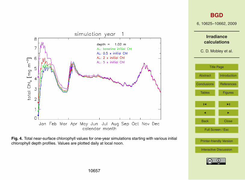
lytic irradiance model. We expect that the long-term ecosystem behavior should bedetermined by the ecosystem internal structure and external forcing, and thus be in-dependent of the initial conditions. To verify this, runs were made starting with theinitial chlorophyll profiles seen in Fig. 3, and with profiles that were one-half, twice, andfive-times the values seen in that figure. Figure 4 shows the resulting total chlorophyll10

concentrations (the sums of the chlorophyll concentrations for the four phytoplanktonfunctional groups) near the sea surface for simulation year 1. For this and subsequentfigures, values are plotted daily at local noon. As expected, the differences due tothe initial chlorophyll profiles damp out within a few months and remain small duringsubsequent years. Greater depths show the same behavior, as do runs using EcoLight-15

computed irradiances.We next examined the ecosystem annual cycle for long-term simulations. A run for

ten simulated years was made starting with the chlorophyll profiles of Fig. 3. The firstthree years show transient behavior as the ecosystem adjusts to the initial profiles andexternal forcing. Years 4–10 then show similar annual cycles, except for a slow year-20

to-year decrease in chlorophyl concentrations, as shown in Fig. 5. During simulationyears 8 to 10, the year-to-year decrease in the annual maximum chlorophyll values is9 to 11% for diatoms and 3 to 5% for dynoflagellates and synechococcus, which givesan annual decrease of about 9% in the maximum total chlorophyll. The annual averagechlorophyll values decrease somewhat less over the same three years, with the annual25

average total chlorophyll (shown by horizontal dotted lines in the figure) decreasing by6.6 to 6.7% each year. This year-to-year decrease in chlorophyll values is a conse-quence of imperfect nutrient replenishment as parameterized by the sinking rates and

10641





BGD6, 10625–10662, 2009


C. D. Mobley et al.

Title Page



Tables Figures

J I

J I

Back Close

Full Screen / Esc



recycling used in EcoSim. The same behavior occurs with EcoLight irradiance calcula-tions. Such behavior is not surprising for the limited spatial grid (which does not includehorizontal advection of nutrients) and fixed particle sinking and nutrient recycling ratesassumed here. The failure of the present idealized ecosystem to attain a completelystable annual cycle in no way compromises our comparisons of analytic vs numerical5

irradiance calculations, for which all else is the same. Although we do not expect toreproduce local conditions within the limited spatial domain, it is encouraging to notethat our modeled surface chlorophyll values in spring-early summer are of the sameorder of magnitude (1–3 mgm−3) as coincident SeaWiFs data for this area.

4 Irradiance model comparisons10

We now consider the long-term ecosystem behavior for different ways of computingthe scalar irradiance used in EcoSim for its primary production calculations. In thesesimulations, the time step was 9 min, which was set by ROMS for computational stabil-ity. A one-year simulation thus requires 58 400 time steps. In the baseline simulations,EcoSim updates its light and biology at each time step, although the irradiances are15

computed only when the sun is above the horizon. Such frequent de novo recompu-tation of the in-water irradiance is not computationally feasible for EcoLight because ofits longer run times, nor is it necessary.

Figure 6 shows a one-year simulation with three versions for the light model calledby EcoSim. The first model is the default analytic light (AL) model used by EcoSim.20

This model computes the irradiances at every grid point (notation: EGP) and everytime step (ETS) when the sun is above the horizon. Irradiances are computed at 5nm resolution between 400 and 700 nm. Irradiances are computed down to the depthwhere the integrated Ed is 1 W m−2. This is the AL baseline run, which is our standardfor comparison with runs that call the EcoLight model to obtain the irradiances. This AL25

run required 32 min on a 2.16 GHz Intel Core Duo iMac running OSX with 1 GB RAM.All run times are totals for the ecosystem simulation and include the physical (ROMS),

10642





BGD6, 10625–10662, 2009


C. D. Mobley et al.

Title Page



Tables Figures

J I

J I

Back Close

Full Screen / Esc



biological (EcoSim) and optical (analytic or EcoLight) calculations.The second model uses EcoLight (EL) to compute the irradiances at every grid point,

every time step, and every wavelength down to a depth where the scalar irradiancedecreased to 0.001 of the surface value, i.e., to a depth zo corresponding to Fo =0.001in Eq. (6), as dynamically corrected by Eq. (7). For the initial chlorophyll profiles seen in5

Fig. 3, zo is approximately 50 m. Below depth zo EcoLight extrapolated the irradiancesusing Eq. (8). This extrapolation defines the irradiances throughout the water column(down to 210 m in these simulations), even though the values at great depths are notused by EcoSim. These EcoLight computations thus give highly accurate irradiancesthroughout the euphotic zone, for the IOP and sky inputs passed to EcoLight by ROMS10

and EcoSim. This full EcoLight simulation corresponds almost exactly to the baselineconditions of the EcoSim calculations using its analytic light model. However, this runrequired 135 h and 35 min, which is much too long for routine calculations.

The third run shown in Fig. 6 shows the results when EcoLight was called at onlyone grid point (1GP) and once per simulation hour (1HR), with other options being the15

same as in the previous EcoLight run. At time steps where EcoLight is not called, themost recently computed spectral irradiances are simply rescaled by the ratio of the cur-rent RADTRAN sky irradiance to that at the time of the previous full computation. Thisshould give good irradiances if the IOPs have not changed greatly since the last fullcalculation. The irradiances at the computed grid point are rescaled in the same man-20

ner and applied at the other grid points. This should give reasonably good predictions ifthe IOPs are not greatly different between the grid points where the exact computationis made and where the rescaled irradiances are applied. This run required 8 h and34 min, which although much faster than the full EL run is still too long for ecosystemmodeling.25

As Fig. 6 shows, the AL base and two EL runs differed by as much as 42% dur-ing the course of the year (computed as 100|AL−EL|/AL). However, the EL full andEL 1GP, 1HR (labeled EL base in the figure) runs were always within one percent ofeach other and are almost indistinguishable in the figure. This shows that EcoLight

10643





BGD6, 10625–10662, 2009


C. D. Mobley et al.

Title Page



Tables Figures

J I

J I

Back Close

Full Screen / Esc



can be called at only one grid point and once per hour without significantly altering theecosystem behavior compared to calling it at every ROMS grid point and every timestep. Compared to the EL full model, the EL 1GP, 1HR, 5 nm, Fo = 0.001 run gives thesame predictions as the EL full model, but at only 6% of the run time. We thereforeadopt these EL options as the baseline for subsequent EcoLight runs for ten-year sim-5

ulations. We presume that the EL runs give a better ecosystem prediction than the ALrun because the EL irradiances are computed more accurately.

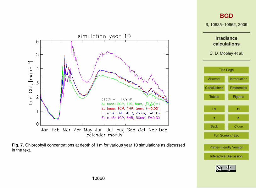
Figure 7 shows several comparisons of AL and EL runs during simulation year 10.We first note the similarity between the AL and EL base runs. (The first year of thissimulation was seen in Fig. 6.) These two runs differ by no more than 23% after ten10

years of simulation. This is a relatively small difference given the much different waysin which the irradiances are computed. The similarity in these two runs can be viewedin either of two ways. First, the agreement is a validation of EcoSim’s simple analyticirradiance model for Case 1 water, compared to the exact solution of the RTE for thesame IOPs. Good agreement is to be expected, since the AL light model was designed15

for use in Case 1 waters as modeled here. Alternatively, the similarity can be viewed asconfirmation that the EcoLight code has been fully debugged and properly embeddedwithin the ROMS-EcoSim code.

Since we can reduce the spatial and temporal frequency of calling EcoLight (or theanalytic light model, for that matter) as just described without altering the ten-year20

ecosystem predictions by more that one percent, the question arises as to how muchmore the frequency of light computations can be reduced without significantly alteringthe long-them ecosystem behavior. Figure 7 shows two further examples of reducedtemporal, wavelength, and depth resolution in EcoLight runs for the last year of a ten-year simulation. EL Run A called EcoLight at the first ROMS time step after sunrise25

and every 4 h (4HR) thereafter each day. Irradiances were computed only at every fifthEcoSim waveband, i.e. at 400, 425, ..., 700 nn, which is 25 nm resolution. Irradiancesat other EcoSim bands were obtained from linear interpolation between the computedbands. Finally, the RTE was solved only down to the 15% light level, i.e., down to

10644





BGD6, 10625–10662, 2009


C. D. Mobley et al.

Title Page



Tables Figures

J I

J I

Back Close

Full Screen / Esc



Fo = 0.15, with extrapolation to deeper depths as previously described. In a similarfashion, EL Run B called EcoLight every 6 h at 50 nm resolution, and solved the RTEdown to only the 50% or Fo =0.5 light level.

The EL base and EL Run A simulations differ by a maximum of 4% during the tenthsimulation year. Thus very little long-term difference was induced by the reduction in5

wavelength and depth resolution for EL Run A vs. the EL base run. However, EL Run Atook only 41 min per simulation year, which is just 28% more than the AL base run. ELRun B took 40 min. The small decrease in run time between EL Run A and Run Bindicates that the overhead required to call and initialize EcoLight now dominates itsrun time, rather than the time required to solve the RTE itself. However, EL Run B10

gives chlorophyll predictions that differ by as much as 73% after ten years, comparedto the EL base run. Note also that the time of the maximum spring bloom is delayed byalmost a month in EL Run B. Such differences are too large to be acceptable. Thus weview the computational frequency of EL Run A as being satisfactory, given the smallincrement in run time compared to the AL model, but EL Run B is not satisfactory and15

in any case gives only a slight additional saving in run time.The same behavior is seen at greater depths. Figure 8 shows the year-ten time

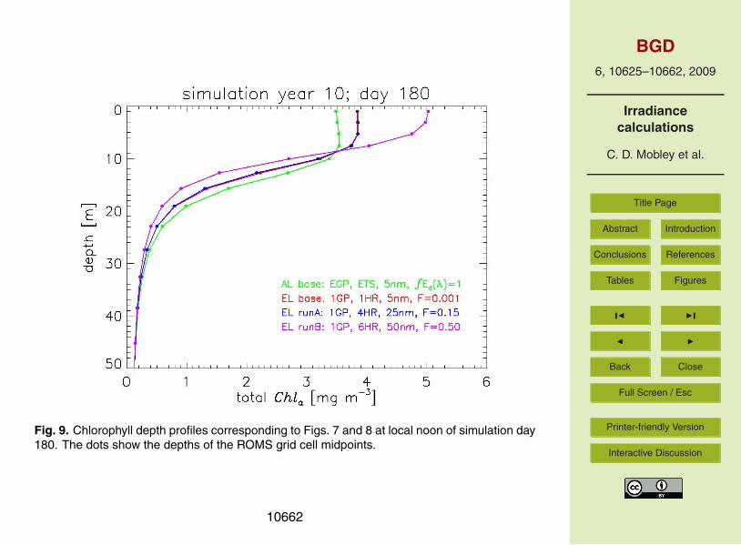
series at depth 15.7 m. At this depth, AL base and EL base differ by up to 26%. ELbase and EL run A remain within 4% of each other, but EL Run B differs from Run Aby up to 65%. Figure 9 shows the upper 50 m depth profile of total chlorophyll values20

at day 180 of year 10, illustrating that the largest difference between the analytical andEcoLight model predictions occurs in the upper 20 m. Below this depth, both solutionsconverge. Table 1 summarizes these runs.

5 Conclusions

It is of course possible to try other combinations of time, wavelength, and depth res-25

olution in EcoLight calls, and we have done so. However, the results presented inFigs. 7–9 are sufficient to show that accurate irradiance calculations can be obtained

10645





BGD6, 10625–10662, 2009


C. D. Mobley et al.

Title Page



Tables Figures

J I

J I

Back Close

Full Screen / Esc



in ecosystem models with at most a few tens of percent increase in total run times.Although both the analytic and EcoLight models gave comparable chlorophyll predic-tions for ten-year simulations of open-ocean Case 1 waters, such agreement cannot beexpected in simulations of Case 2 waters, for which the analytic light model is not valid.The EcoLight solution of the RTE to a given optical depth is not dependent on whether5

the IOPs describe Case 1 or 2 water. Its fast run times seen here will therefore beretained in applications to other water bodies. A chlorophyll-based analytic light modelwill underestimate the scalar irradiance in simulations of optically shallow waters withbright reflective bottoms. In such waters, bottom reflectance increases the in-waterscalar irradiance and proportionately affects biological productivity and water-column10

heating rates. In optically shallow waters, it would be necessary to force EcoLight tosolve the RTE all the way to the physical bottom at each wavelength in order to accountfor bottom reflectance effects. However, any corresponding increase in run time is apenalty worth paying if the improved irradiance computations give significantly betterecosystem predictions in such waters, and the run time will even decrease if the bottom15

depth is less than the deep-water zo given by Eq. (7).It is our view that it does not matter how fast a light model runs if its predictions are

not sufficiently accurate to meet the user’s needs. EcoLight provides a numerical lightmodel that accurately computes irradiances for any water body or boundary conditionsbeing simulated by the associated physical-biological models. The run time increase20

when using EcoLight in an optimized way, i.e., not calling it at every time step, everygrid point, and every wavelength, is at most a few tens of percent. Moreover, EcoLightautomatically provides ancillary output (not shown in this paper) such as the remotesensing reflectance, plane irradiances, and nadir- and zenith-viewing radiances, all ofwhich can be used to verify ecosystem predictions with observational data, or which25

may be of use for other purposes such as estimation of underwater visibility. Suchancillary data are not provided by the analytic light model. The use of an RTE-basedoptical model also facilitates data assimilation into the ecosystem model when IOPor related measurements are available. EcoLight’s extra computational time is a small

10646





BGD6, 10625–10662, 2009


C. D. Mobley et al.

Title Page



Tables Figures

J I

J I

Back Close

Full Screen / Esc



price to pay for potential improvements in ecosystem predictions, for extending the lightmodel to Case 2 and shallow waters, and for obtaining ancillary radiometric variablesuseful for ecosystem validation.

We thus feel that although simple analytic irradiance models do run extremely fast,there is little justification for their continued use in light of their potential inaccuracies5

and limitations, even for Case 1 waters. Moreover, analytic models usually parameter-ize the water inherent optical properties in terms of a single quantity – the total chloro-phyll concentration – which oversimplifies the complex relation between light propaga-tion and the scattering and absorption properties of various ocean constituents. So-phisticated ecosystem models such as EcoSim track several phytoplankton functional10

groups as well as other dissolved and particulate constituents, each of which has itsown absorption and scattering properties. EcoSim determines total inherent opticalproperties as sums of the contributions by various components and is thus able tomodel changes in the light field induced by changes in the concentration or opticalproperties of whatever components are included in the biological model. Such connec-15

tions between ecosystem components and the light field cannot be well simulated bychlorophyll-based models.

Computational stability criteria of ecosystem physical models may require time stepsas small as one minute, depending on grid cell size. However, it is seldom if ever nec-essary to update the light field at each time step. It appears reasonable to run EcoLight20

at hourly or longer intervals and then interpolate to the desired time. The same ideaapplies to running EcoLight on a coarser spatial grid than the physical model uses andthen interpolating to obtain the required spatial resolution. In practice, it should be pos-sible to dynamically determine when to call EcoLight. For example, as the calculationsproceed to a new grid point, the IOPs at that grid point could be compared with those25

at the last grid point where EcoLight was called (the reference point). If the IOPs atthe new grid point differ by less than some amount from those at the reference point,then the previously computed irradiances would be rescaled, as was done with the1GP calculations studied here, and applied at the new grid point. If the IOPs at the

10647





BGD6, 10625–10662, 2009


C. D. Mobley et al.

Title Page



Tables Figures

J I

J I

Back Close

Full Screen / Esc



new grid point differ by more than some amount from those at the reference point, thenEcoLight would be called for a de novo calculation of the irradiance, and the currentgrid point would become the new reference point. A dynamic determination of when tocall EcoLight would allow for frequent calls near fronts or in other situations where theIOPs or external properties are changing rapidly, and for few calls in fairly homogenous5

and stable ocean regions. When employed is this manner, EcoLight should be applica-ble to large-scale three-dimensional ecosystem models requiring spectral irradiancesat many wavelengths and on a fine spatial and temporal grid, but at little more compu-tational expense than calling an analytical light model at every time step and grid point,as is done in the current ROMS-EcoSim code.10

Light is an important factor in determining primary production and mixed-layer ther-modynamics, so we expect that EcoLight’s accurately computed spectral scalar irra-diances will significantly improve ecosystem model predictions, compared to the useof approximate analytical models for spectral irradiance or PAR. Moreover, predictionsof primary production in shallow waters and for sea grass beds, for which analytic15

chlorophyll-based models can be off by large factors, would be well-served by the useof EcoLight.

The EcoLight version 1.0 code used in the present study is mostly Fortran 77 andcontains HydroLight legacy features that are not needed for ecosystem simulations.We expect that a thorough rewriting of EcoLight in Fortran 95, removal of unneeded20

features, and use of a faster RTE solver might gain another factor of two in run timesfor the EcoLight module. That rewrite is now under way. When ready, that code will beimbedded in a fully 3-D ecosystem model for investigation of the issues just mentioned.

Acknowledgements. Authors C. D. M. and L. K. S. were supported in this work by the US Officeof Naval Research Environmental Optics Program as part of the Hyperspectral Coastal Ocean25

Dynamics Experiment (HyCODE) and under follow-on contracts N00014-00-D-0161, N00014-05-M-0146, and N00014-8-C-0024. Authors W. P. B. and B. C. were supported by Office ofNaval Research Environmental Optics Program as part of HyCODE, under follow-on contractN00014-8-C-0024, and by the US National Science Foundation Coastal Ocean Processes La-grangian Transport and Transformation Experiment (LaTTE) under grant 0238745.30

10648





BGD6, 10625–10662, 2009


C. D. Mobley et al.

Title Page



Tables Figures

J I

J I

Back Close

Full Screen / Esc



References

Baker, K. S. and Frouin, R.: Relation between photosynthetically available radiation and totalinsolation at the ocean surface under clear skies, Limnol. Oceanogr., 32, 1370–1377, 1987.10629

Bissett, W. P., Meyers, M. B., Walsh. J. J., and Muller-Karger, F. E: The effects of temporal5

variability of mixed layer depth on primary productivity around Bermuda, J. Geophys. Res.,99(C4), 7539–7553, 1994. 10627

Bissett, W. P., Walsh, J. J., Dieterle, D. A., and Carder, K. L.: Carbon cycling in the upper watersof the Sargasso Sea: I. Numerical simulation of differential carbon and nitrogen fluxes, Deep-Sea Res., 46, 205–269, 1999a. 10629, 10632, 1063310

Bissett, W. P., Carder, K. L., Walsh, J. J., and Dieterle, D. A.: Carbon cycling in the upper watersof the Sargasso Sea: II. Numerical simulation of apparent and inherent optical properties,Deep-Sea Res., 46, 271–317, 1999b. 10629, 10632, 10634

Bissett, W. P, Schofield, O., Glenn, S., Cullen, J. J., Miller, W. L., Plueddemann, A. J., andMobley, C. D.: Resolving the impacts and feedbacks of ocean optics on upper ocean ecology.15

Oceanography, 14, 30–49, 2001.Bissett, W. P., DeBra, S., and Dye, D.: Ecological Simulation (EcoSim) 2.0 Technical De-

scription. FERI Technical Document Number FERI-2004-0002-U-D, online available at: http://feri.s3.amazonaws.com/pubs ppts/FERI 2004 0002 U D.pdf, 10 August, 2004. 10633

Bissett, W. P., Arnone, R., DeBra, S., Dieterle, D. A., Dye, D., Kirkpatrick, G., Schofield, O.20

M., and Vargo, G.: Predicting the optical properties of the West Florida Shelf: Resolving thepotential impacts of a terrestrial boundary condition on the distribution of colored dissolvedand particulate matter, Mar. Chem., 95, 199–233, 2005. 10632

Bissett, W. P., Arnone, R., DeBra, S., Dye, D., Kirkpatrick, G., Mobley, C. D., and Schofield, O.M.: The integration of ocean color remote sensing with coastal nowcast/forecast simulations25

of harmful algal blooms (HABs), in: Real Time Coastal Observing Systems for EcosystemDynamics and Harmful Algal Blooms, edited by: Babin, M., Roesler, C., and Cullen, J. J., UNEduc., Sci. and Cult. Organ., Paris, 85–108, 2008. 10632

Cahill, B., Schofield, O., Chant, R., Wilkin, J., Hunter, E., Glenn, S., and Bissett, W. P.: Dynam-ics of turbid buoyant plumes and the feedbacks on nearshore biogeochemistry and physics,30

Geophys. Res. Lett., 35, L10605, doi:10.1029/2008GL033595, 2008. 10631Dinniman, M. S., Klinck, J. M., and Smith Jr., W. O. : Cross shelf exchange in a model of the

10649





http://feri.s3.amazonaws.com/pubs_ppts/FERI_2004_0002_U_D.pdf



BGD6, 10625–10662, 2009


C. D. Mobley et al.

Title Page



Tables Figures

J I

J I

Back Close

Full Screen / Esc



Ross Sea circulation and biogeochemistry, Deep-Sea Res. II, 50, 3103–3120, 2003. 10631Doney, S. C., Glover, D. M., and Najjar, R. G.: A new coupled, one-dimensional biological-

physical model for the upper ocean: Application to the JGOFS Bermuda Atlantic TimeseriesStudy (BATS) site, Deep-Sea Res. II, 43, 591–624, 1996. 10628

Eppley, R. W.: Temperature and phytoplankton growth in the sea, Fish. Bull., 70(4), 1063–1085,5

1972. 10632Evans, G. T. and Parslow, J. S.: A model of annual plankton cycles, Biol. Oceanogr., 3, 328–

347, 1985. 10627, 10628Fasham, M. J. R.: Variations in the seasonal cycle of biological production in subarctic oceans:

A model sensitivity analysis, Deep-Sea Res. II, 42, 1111–1149, 1995. 1062810

Fasham, M. J. R., Ducklow, H. W., and McKelvie, S. M.: A nitrogen-based model of planktondynamics in the oceanic mixed layer, J. Mar. Res., 48, 591–639, 1990. 10628

Fennel, K. and Wilkin, J.: Quantifying biological carbon export for the northwest North A tlanticcontinental shelves, Geophys. Res. Lett., in press, 2009. 10631

Fennel, K., Wilkin, J., Levin, J., Moisan, J., O’Reilly, J., and Haidvogel, D.: Nitrogen cy-15

cling in the Middle Atlantic Bight: Results from a three-dimensional model and impli-cations for the North Atlantic nitrogen budget, Global Biogeochem. Cy., 20, GB3007,doi:10.1029/2005GB002456, 2006. 10631

Fennel, K., Wilkin, J., Previdi, M., and Najjar, R.: Denitrification effects on air-sea CO2 flux inthe coastal ocean: Simulations for the Northwest North Atlantic, Geophys. Res. Lett., 35,20

L24608, doi:10.1029/2008GL036147, 2008. 10631Fringer, O. B, McWilliams, J. C., and Street, R. L.: A new hybrid model for coastal simulations,

Oceanography, 19, 64–77, 2006.Fujii, M., Boss, E., and Chai, F.: The value of adding optics to ecosystem models: a case study,

Biogeosciences, 4, 817–835, 2007,25

http://www.biogeosciences.net/4/817/2007/. 10630Gordon, H. R. and Morel, A.: Remote assessment of ocean color for interpretation of satel-

lite visible imagery, a review, Lecture Notes on Coastal and Estuarine Studies, 4, SpringerVerlag, New York, 114 pp., 1983. 10634

Gregg, W. W. and Carder, K. L.: A simple spectral solar irradiance model for cloudless maritime30

atmospheres, Limnol. Oceanogr., 35, 1657–1675, 1990. 10633Hurtt, G. C. and Armstrong, R. A.: A pelagic ecosystem model calibrated with BATS data,

Deep-Sea Res. II, 43, 653–683, 1996. 10628

10650





http://www.biogeosciences.net/4/817/2007/

BGD6, 10625–10662, 2009


C. D. Mobley et al.

Title Page



Tables Figures

J I

J I

Back Close

Full Screen / Esc



Kyewalyanga, M., Platt, T., and Sathyendranath, S.: Ocean primary production calculated byspectral and broad-band models, Mar. Ecol.-Prog. Ser., 85, 171–185, 1992. 10628

Liu, C.-C., Woods, J. D., and Mobley, C. D.: Optical model for use in oceanic ecosystem models,Appl. Optics, 38, 4475–4485, 1999. 10636

Liu, C.-C., Carder, K. L., Miller, R. L., and Ivey, J. E.: Fast and accurate model of underwater5

scalar irradiance, Appl. Optics, 41, 4962-4974, 2002. 10636Lutjeharms, J. R. E., Penven, P., and Roy, C.: Modelling the shear edge eddies of the southern

Agulhas Current, Cont. Shelf Res., 23, 1099–1115, 2003. 10631Marchesiello, P., McWilliams, J. C., and Shchepetkin, A. F.: Equilibrium structure and dynamics

of the California Current System, J. Phys. Oceanogr., 33(4), 753–783, 2003. 1063110

Mobley, C. D.: Light and Water: Radiative Transfer in Natural Waters, Academic Press, SanDiego, 1994. 10626, 10630, 10635, 10638

Mobley, C. D., Gentili, B., Gordon, H. R., Jin, Z., Kattawar, G. W., Morel, A., Reinersman, P.,Stamnes, K., and Stavn, R. H.: Comparison of numerical models for computing underwaterlight fields, Appl. Optics, 32, 7484–7504, 1993. 10630, 1063515

Moore, J. K, Doney, S. C., Kleypas, J. A., Glover, D. M., and Fung, I. Y.: An intermediatecomplexity marine ecosystem model for the global domain, Deep-Sea Res. II, 49, 403–462,2002. 10628

Morel, A. and Maritorena, S.: Bio-optical properties of oceanic waters: a reappraisal, J. Geo-phys. Res., 106(C4), 7163–7180, 2001. 1063420

Oguz, T., Ducklow, H., Malanotte-Rizzoli, P., Tugrul, S., Nezlin, N. P., and Unluata, U.: Simu-lation of annual plankton productivity cycle in the Black Sea by a one-dimensional physical-biological model, J. Geophys. Res., 101, 16585–16599, 1996. 10628

Oschlies, A. and Garcon, V.: An eddy-permitting coupled physical-biological model of theNorth Atlantic - Part I: Sensitivity to advection numerics and mixed layer physics, Global25

Biogeochem. Cy., 13, 135–160, 1998. 10628Paulson, C. A. and Simpson, J. J.: Irradiance measurements in the upper ocean, J. Phys.

Oceanogr., 7, 952–956, 1977.Peliz, A., Dubert, J., Haidvogel, D. B., and Le Cann, B.: Generation and unstable evolution of

a density-driven eastern poleward current: The Iberian Poleward Current, J. Geophys. Res.,30

108(C8), 3268, doi:10.1029/2002JC001443, 2003. 10631Sakshaug, E., Bricaud, A., Dandonneau, Y., Falkowski, P. G., Kiefer, D. A., Legendre, L., Morel,

A., Parslow, J., and Takahashi, M.: Parameters of photosynthesis: definitions, theory, and

10651





BGD6, 10625–10662, 2009


C. D. Mobley et al.

Title Page



Tables Figures

J I

J I

Back Close

Full Screen / Esc



interpretation of results, J. Plankton Res., 19, 1637–1670, 1997. 10627Shchepetkin, A. and McWilliams, J. C.: Quasi-monotone advection schemes based on explicit

locally adaptive dissipation, Mon. Weather Rev., 126, 1541–1580, 1998. 10631Shchepetkin, A. and McWilliams, J. C.: A method for computing horizontal pressure gradient

force in an oceanic model with a nonaligned vertical coordinate, J. Geophys. Res., 108, 3090,5

doi:10.1029/2001JC001047, 2003. 10631Shchepetkin, A. F. and McWilliams, J. C.: The regional ocean modeling system (ROMS): a

split-explicit, free-surface, topography-following-coordinate oceanic model, Ocean Model., 9,347–404, 2005. 10631

Simpson, J. J. and Dickey, T. D.: Alternative parameterizations of downward irradiance and10

their dynamical significance, J. Phys. Oceanogr., 11, 876–882, 1981. 10629Steele, J. H. and Henderson, E. W.: The role of predation in plankton models, J. Plankton Res.,

14(1), 157–172, 1992. 10632Wilkin, J. L.: The summertime heat budget and circulation of southeast New England shelf

waters, J. Phys. Oceanogr., 36(11), 1997–2011, 2006. 1063115

Zielinski, O., Oschlies, A., and Reuter, R.: Comparison of underwater light field parameteriza-tions and their effect on a 1-dimensional biogeochemical model at Station ESTOC, north ofthe Canary Islands, in: Proceedings Ocean Optics XIV, P. Soc. Photo-opt. Ins., Kona-Kailua,Hawaii, 1998. 10628, 10629

10652





BGD6, 10625–10662, 2009


C. D. Mobley et al.

Title Page



Tables Figures

J I

J I

Back Close

Full Screen / Esc



Table 1. Options used in comparison runs. Time resolution of 9 min is every ROMS time step;grid resolution of EGP is every ROMS grid point; wavelength resolution of 5 nm is every EcoSimwavelength. The run times are per year of simulation on a 2.16 GHz iMac computer.

modeltime

resolutiongrid

resolution

depthresolutionFo of Eq.(6)

wavelengthresolution

run time persimulation year

hr:min

Analytic 9 min EGP NA 5 nm 0:32EcoLight full 9 min EGP 0.001 5 nm 135:35EcoLight base every hour 1 grid point 0.001 5 nm 8:34EcoLight Run A every 4 h 1 grid point 0.15 25 nm 0:41EcoLight Run B every 6 h 1 grid point 0.5 50 nm 0:40

10653





BGD6, 10625–10662, 2009


C. D. Mobley et al.

Title Page



Tables Figures

J I

J I

Back Close

Full Screen / Esc



Fig. 1. The ROMS computational grid. The open circle grid points are used to apply the periodicboundary conditions. Biological computations are performed at the 4×4 interior grid shown bythe solid symbols. Output in subsequent figures is plotted at the square. EcoLight runs thatcompute the light only at one grid point are done at the diamond.

10654





BGD6, 10625–10662, 2009


C. D. Mobley et al.

Title Page



Tables Figures

J I

J I

Back Close

Full Screen / Esc



Fig. 2. Short-wave local-noon irradiances used in ROMS. This annual cycle was repeated foreach year of the simulation.

10655





BGD6, 10625–10662, 2009


C. D. Mobley et al.

Title Page



Tables Figures

J I

J I

Back Close

Full Screen / Esc



Fig. 3. The baseline initial depth profiles of Chla for the four functional groups, and their total.

10656





BGD6, 10625–10662, 2009


C. D. Mobley et al.

Title Page



Tables Figures

J I

J I

Back Close

Full Screen / Esc



Fig. 4. Total near-surface chlorophyll values for one-year simulations starting with various initialchlorophyll depth profiles. Values are plotted daily at local noon.

10657





BGD6, 10625–10662, 2009


C. D. Mobley et al.

Title Page



Tables Figures

J I

J I

Back Close

Full Screen / Esc



Fig. 5. Time series of surface chlorophyll for the ten-year baseline simulation using the analyticlight model in EcoSim. The horizontal red dotted lines are the annual average total chlorophyllvalues within each simulation year. The vertical black dotted lines are at 31 December of eachyear.

10658





BGD6, 10625–10662, 2009


C. D. Mobley et al.

Title Page



Tables Figures

J I

J I

Back Close

Full Screen / Esc



Fig. 6. Chlorophyll concentrations at depth of 1 m for various year 1 simulations as discussedin the text.

10659





BGD6, 10625–10662, 2009


C. D. Mobley et al.

Title Page



Tables Figures

J I

J I

Back Close

Full Screen / Esc



Fig. 7. Chlorophyll concentrations at depth of 1 m for various year 10 simulations as discussedin the text.

10660





BGD6, 10625–10662, 2009


C. D. Mobley et al.

Title Page



Tables Figures

J I

J I

Back Close

Full Screen / Esc



Fig. 8. Chlorophyll concentrations at depth of 15.7 m for various year 10 simulations as dis-cussed in the text.

10661





BGD6, 10625–10662, 2009


C. D. Mobley et al.

Title Page



Tables Figures

J I

J I

Back Close

Full Screen / Esc



Fig. 9. Chlorophyll depth profiles corresponding to Figs. 7 and 8 at local noon of simulation day180. The dots show the depths of the ROMS grid cell midpoints.

10662





Fast and accurate irradiance calculations for … 6, 10625–10662, 2009 Irradiance calculations C....

Documents

Transcript of Fast and accurate irradiance calculations for … 6, 10625–10662, 2009 Irradiance calculations C....