Far-field Measurements of Seismic Airgun Array Pulses in the Nova Scotia Gully Marine Protected Area Ian H. McQuinn and Dominic Carrier Hydroacoustic Laboratory Maurice Lamontagne Institute Department of Fisheries and Oceans 850, route de la Mer Mont-Joli, Québec, Canada G5H 3Z4 2005

Canadian Technical Report of Fisheries and Aquatic Sciences 2615

Pêches et Océans Canada

Fisheries and Oceans Canada

Canadian Technical Report of Fisheries and Aquatic Sciences

Technical reports contain scientific and technical information that contributes to existing knowledge but which is not normally appropriate for primary literature. Technical reports are directed primarily toward a worldwide audience and have an international distribution. No restriction is placed on subject matter and the series reflects the broad interests and policies of Fisheries and Oceans Canada, namely, fisheries and aquatic sciences.

Technical reports may be cited as full publications. The correct citation appears above the abstract of each report. Each report is abstracted in the data base Aquatic Sciences and Fisheries Abstracts.

Technical reports are produced regionally but are numbered nationally. Requests for individual reports will be filled by the issuing establishment listed on the front cover and title page.

Numbers 1-456 in this series were issued as Technical Reports of the Fisheries Research Board of Canada. Numbers 457-714 were issued as Department of the Environment, Fisheries and Marine Service, Research and Development Directorate Technical Reports. Numbers 715-924 were issued as Department of Fisheries and Environment, Fisheries and Marine Service Technical Reports. The current series name was changed with report number 925.

Rapport technique canadien des sciences halieutiques et aquatiques

Les rapports techniques contiennent des renseignements scientifiques et techniques qui constituent une contribution aux connaissances actuelles, mais qui ne sont pas normalement appropriés pour la publication dans un journal scientifique. Les rapports techniques sont destinés essentiellement à un public international et ils sont distribués à cet échelon. II n'y a aucune restriction quant au sujet; de fait, la série reflète la vaste gamme des intérêts et des politiques de Pêches et Océans Canada, c'est-à-dire les sciences halieutiques et aquatiques.

Les rapports techniques peuvent être cités comme des publications à part entière. Le titre exact figure au-dessus du résumé de chaque rapport. Les rapports techniques sont résumés dans la base de données Résumés des sciences aquatiques et halieutiques.

Les rapports techniques sont produits à l'échelon régional, mais numérotés à l'échelon national. Les demandes de rapports seront satisfaites par l'établissement auteur dont le nom figure sur la couverture et la page du titre.

Les numéros 1 à 456 de cette série ont été publiés à titre de Rapports techniques de l'Office des recherches sur les pêcheries du Canada. Les numéros 457 à 714 sont parus à titre de Rapports techniques de la Direction générale de la recherche et du développement, Service des pêches et de la mer, ministère de l'Environnement. Les numéros 715 à 924 ont été publiés à titre de Rapports techniques du Service des pêches et de la mer, ministère des Pêches et de l'Environnement. Le nom actuel de la série a été établi lors de la parution du numéro 925.

i

Canadian Technical Report of Fisheries and Aquatic Sciences 2615

2005

FAR-FIELD MEASUREMENTS OF SEISMIC AIRGUN ARRAY PULSES IN THE NOVA SCOTIA GULLY MARINE PROTECTED AREA

by

Ian H. McQuinn and Dominic Carrier1

Hydroacoustic Laboratory Maurice Lamontagne Institute

Department of Fisheries and Oceans 850, route de la Mer

Mont-Joli, Québec, Canada G5H 3Z4

E-mail: mcquinni@dfo-mpo.gc.ca

1 Physics Department, Sherbrooke University, Sherbrooke, Quebec, J1K 2R1

ii

© Her Majesty the Queen in Right of Canada, 2005. Cat. No. Fs 97-6/2615E ISSN 1488-5379

Correct citation for this publication: McQuinn, I.H. and Carrier D. 2005, Far-field Measurements of Seismic Airgun Array

Pulses in the Nova Scotia Gully Marine Protected Area. Can. Tech. Rep. Fish. Aquat. Sci. 2615: v + 20 p.

iii

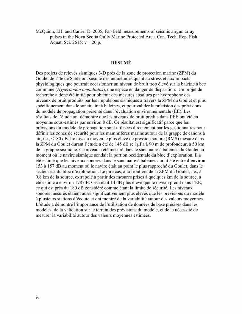
McQuinn, I.H. and Carrier D. 2005, Far-field measurements of seismic airgun array pulses in the Nova Scotia Gully Marine Protected Area. Can. Tech. Rep. Fish. Aquat. Sci. 2615: v + 20 p.

ABSTRACT

Plans for conducting 3-D seismic exploration adjacent to the Sable Island Gully Marine Protected Area (MPA) prompted concerns over the potential for stress or physiological harm to the endangered northern bottlenose whale (Hyperoodon ampullatus) from the increased noise levels. A study of the far-field measurement of seismic pulses throughout the Gully MPA and specifically the Gully Whale Sanctuary was therefore initiated to directly measure noise levels produced by the seismic pulses and to validate the accuracy of sound propagation predictions published in the environmental assessment (EA). Our results showed that the noise levels predicted in the EA were on average underestimated by 8 dB. This finding is significant since the results of sound propagation models are used by regulators to define the safety radius for marine mammals around seismic arrays, i.e., <180 dB. The highest average sound pressure level (RMS) measured in the Gully MPA during the present study was 145 dB re 1µPa at 90 m depth, 50 km from the seismic array. This sound level was measured within the Gully Whale Sanctuary while the seismic vessel was surveying the western portion of the exploration block. It was estimated that sound levels in the Whale Sanctuary would have been between approximately 153 and 157 dB when the vessel was at its closest approach to the Gully in the eastern portion of the survey block. The “worst case” sound level at the Gully MPA boundary, i.e., 0.8 km from the source, extrapolated from near-field measurements would have been approximately 178 dB, 14 dB higher than originally predicted in the EA and close to the 180 dB safety criteria. Measured sound levels were also significantly higher than the model predictions at several other stations and showed significant variability around the mean values. This demonstrates the importance of using accurate model input data, of using field validation to verify the model predictions and of the need to measure the variability around the mean sound level estimates.

iv

McQuinn, I.H. and Carrier D. 2005, Far-field measurements of seismic airgun array pulses in the Nova Scotia Gully Marine Protected Area. Can. Tech. Rep. Fish. Aquat. Sci. 2615: v + 20 p.

RÉSUMÉ

Des projets de relevés sismiques 3-D près de la zone de protection marine (ZPM) du Goulet de l’île de Sable ont suscité des inquiétudes quant au stress et aux impacts physiologiques que pourrait occasionner un niveau de bruit trop élevé sur la baleine à bec commune (Hyperoodon ampullatus), une espèce en danger de disparition. Un projet de recherche a donc été initié pour obtenir des mesures absolues par hydrophone des niveaux de bruit produits par les impulsions sismiques à travers la ZPM du Goulet et plus spécifiquement dans le sanctuaire à baleines, et pour valider la précision des prévisions du modèle de propagation présenté dans l’évaluation environnementale (ÉE). Les résultats de l’étude ont démontré que les niveaux de bruit prédits dans l’ÉE ont été en moyenne sous-estimés par environ 8 dB. Ce résultat est significatif parce que les prévisions du modèle de propagation sont utilisées directement par les gestionnaires pour définir les zones de sécurité pour les mammifères marins autour de la grappe de canons à air, i.e., <180 dB. Le niveau moyen le plus élevé de pression sonore (RMS) mesuré dans la ZPM du Goulet durant l’étude a été de 145 dB re 1µPa à 90 m de profondeur, à 50 km de la grappe sismique. Ce niveau a été mesuré dans le sanctuaire à baleines du Goulet au moment où le navire sismique sondait la portion occidentale du bloc d’exploration. Il a été estimé que les niveaux sonores dans le sanctuaire à baleines aurait été entre d’environ 153 à 157 dB au moment où le navire était au point le plus rapproché du Goulet, dans le secteur est du bloc d’exploration. Le pire cas, à la frontière de la ZPM du Goulet, i.e., à 0,8 km de la source, extrapolé à partir des mesures prises à quelques km de la source, a été estimé à environ 178 dB. Ceci était 14 dB plus élevé que le niveau prédit dans l’ÉE, ce qui est près du 180 dB considéré comme étant la limite de sécurité. Les niveaux sonores mesurés étaient aussi significativement plus élevés que les prévisions du modèle à plusieurs stations d’écoute et ont montré de la variabilité autour des valeurs moyennes. L’étude a démontré l’importance de l’utilisation de données de base précises dans les modèles, de la validation sur le terrain des prévisions du modèle, et de la nécessité de mesurer la variabilité autour des valeurs moyennes estimées.

1

INTRODUCTION

Interest in seismic oil and gas exploration on the Scotian Shelf off Nova Scotia has been increasing in recent years, with the submission of proposals for seismic surveys in previously unexplored deep-water areas and new licenses being issued. However, the recent designation of the Sable Island Gully as a Marine Protected Area (MPA) has prompted calls for increased vigilance on the part of regulatory bodies when issuing licences near this sensitive area. The Gully MPA is an ecologically significant habitat for many marine mammals and includes a whale sanctuary (Figure 1) principally for the

northern bottlenose whale (NBW), Hyperoodon ampullatus, listed as an endangered species under COSEWIC (Committee on Status of Endangered Wildlife in Canada). Concerns have been raised over the potential impacts of loud noise sources such as seismic airgun arrays on the physiology and behaviour of marine mammals and in particular on special status species such as the NBW, which has its main distribution in and around the Gully MPA (Whitehead et al., 1997) and the adjacent Shortland and Haldimand marine canyons of the outer Scotian Shelf and Scotian Slope. There was therefore considerable concern over the increased noise levels produced within the Gully MPA from 3-D seismic shooting in adjacent exploration blocks leased by Marathon Canada Ltd. and EnCana Corporation and the potential for stress and physiological harm to the NBW.

Figure 1. Location of the Marathon exploration block relative to known northern bottlenose whale

habitat in the Gully MPA and the Shortland and Haldimand canyons.

2

Worldwide, regulatory bodies are relying on mitigation measures to lessen the impacts of seismic exploration on marine life, with particular attention to marine mammals. One of the principle mitigation measures used during seismic surveys is the definition of one or more safety zones around the array that define areas of potential physiological and behavioural impact upon marine mammals. Typically, operators may be required to cease shooting if a marine mammal is sighted within a safety zone defined as a radius around the seismic array within which the received sound pressure level (SPL) is predicted to be above a given criteria. In the case of the Marathon Canada Ltd. project, estimated sound levels were calculated for the environmental assessment (EA) from a sound propagation model for various trajectories from sources within the Marathon licence block to receive points in the near-field (i.e., within hundreds of meters of the vessel) and in the far-field, including the Gully MPA (Moulton et al., 2003). The safety radius for cetaceans was determined from these models to be 500 m for a received level of 180 dB re 1 µPa (RMS).

The Gully Seismic Research Program was initiated by Fisheries and Oceans Canada in partnership with the industry to study the propagation of seismic pulses into the Gully MPA from the Marathon 3D seismic survey. The present study focused on measuring seismic airgun array sound levels in the far-field throughout the Gully MPA and on validating the accuracy of far-field sound propagation model predictions from the environmental assessment (Moulton et al., 2003).

MATERIAL AND METHODS

Our study was initially planned to measure far-field (> 30 km) ambient noise before seismic shooting and sound levels when the seismic array was shooting closest to the Gully MPA. However, due to significant delays, the 90-day Marathon seismic reflection survey began several months later than scheduled. Therefore the two studies were rescheduled, one before the seismic survey (April, 2003) to measure ambient noise and to record marine mammal vocalizations and the other during seismic shooting (July, 2003) to measure the far-field seismic noise levels, ambient noise and again to record marine mammal vocalizations. However, at this time, the seismic vessel M/V Ramform Viking was at the western extremity of the Marathon block, some 30 km from the Gully MPA at its closest approach.

The CRV Strait Signet was chartered as a platform for conducting the noise recordings and for the marine mammal observations. A surface deployed calibrated hydrophone recording system called RUSTLER (Hydroacoustic Laboratory, MLI, DFO, Mont-Joli, Qc) was used for sound data collection. This system was powered from two 12-volt batteries and consisted of an omni-directional (± 1 dB) ITC6050 recording hydrophone (midband receive sensitivity: -157 dB V/µPa), a Reson TC4033 reference hydrophone, a Reson TP1000 fixed gain/highpass filter (1 Hz) and a Marantz PMD670 microdrive recorder. The recording and reference hydrophones were calibrated at the Hydroacoustic Laboratory, MLI, referenced to a pistophone-calibrated B&K 8105 hydrophone. The TC4033 reference hydrophone produced a 2-sec, 10 kHz tone at 2.5-min intervals that was used to validate the system calibration coefficients after deployment. This avoids having to recalibrate the system when a component is replaced, provides a means to

3

ensure that the receive hydrophone is stable over time, ensures that the system amplitude corresponds to the recorded gain settings and can be used to diagnose trouble with the system or to provide warning of problems as they develop (e.g., leaks in the cable).

The frequency response of all components was measured in the laboratory and was used to normalize the sound recordings. Recordings were stored in standard PCM wav format with a bandwidth of 24,000 Hz, i.e., at a sampling rate of 48,000 samples/sec. GPS position data was collected on both vessels and referenced to the GPS time for the estimation of transmission ranges.

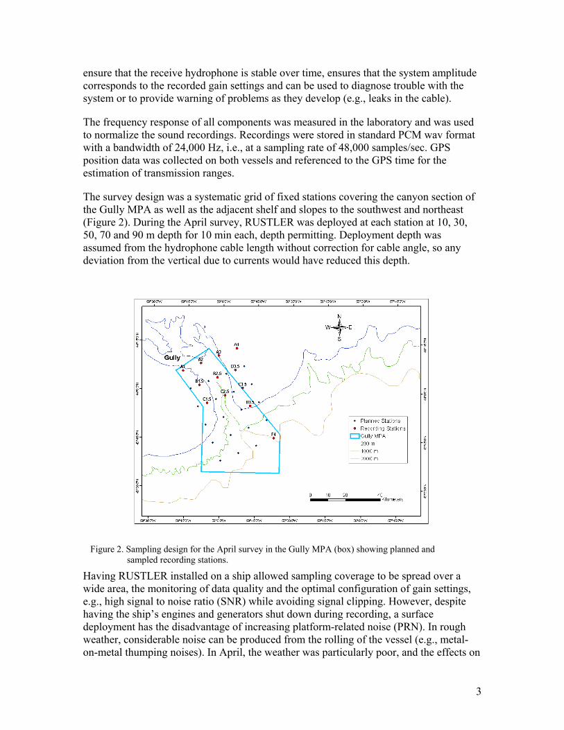
The survey design was a systematic grid of fixed stations covering the canyon section of the Gully MPA as well as the adjacent shelf and slopes to the southwest and northeast (Figure 2). During the April survey, RUSTLER was deployed at each station at 10, 30, 50, 70 and 90 m depth for 10 min each, depth permitting. Deployment depth was assumed from the hydrophone cable length without correction for cable angle, so any deviation from the vertical due to currents would have reduced this depth.

Having RUSTLER installed on a ship allowed sampling coverage to be spread over a wide area, the monitoring of data quality and the optimal configuration of gain settings, e.g., high signal to noise ratio (SNR) while avoiding signal clipping. However, despite having the ship’s engines and generators shut down during recording, a surface deployment has the disadvantage of increasing platform-related noise (PRN). In rough weather, considerable noise can be produced from the rolling of the vessel (e.g., metal-on-metal thumping noises). In April, the weather was particularly poor, and the effects on

Figure 2. Sampling design for the April survey in the Gully MPA (box) showing planned and

sampled recording stations.

4

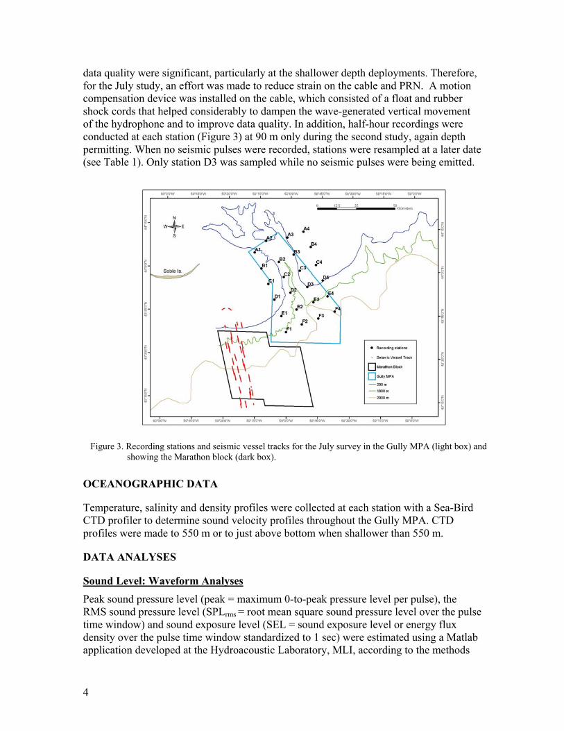
data quality were significant, particularly at the shallower depth deployments. Therefore, for the July study, an effort was made to reduce strain on the cable and PRN. A motion compensation device was installed on the cable, which consisted of a float and rubber shock cords that helped considerably to dampen the wave-generated vertical movement of the hydrophone and to improve data quality. In addition, half-hour recordings were conducted at each station (Figure 3) at 90 m only during the second study, again depth permitting. When no seismic pulses were recorded, stations were resampled at a later date (see Table 1). Only station D3 was sampled while no seismic pulses were being emitted.

OCEANOGRAPHIC DATA

Temperature, salinity and density profiles were collected at each station with a Sea-Bird CTD profiler to determine sound velocity profiles throughout the Gully MPA. CTD profiles were made to 550 m or to just above bottom when shallower than 550 m.

DATA ANALYSES

Sound Level: Waveform Analyses Peak sound pressure level (peak = maximum 0-to-peak pressure level per pulse), the RMS sound pressure level (SPLrms = root mean square sound pressure level over the pulse time window) and sound exposure level (SEL = sound exposure level or energy flux density over the pulse time window standardized to 1 sec) were estimated using a Matlab application developed at the Hydroacoustic Laboratory, MLI, according to the methods

Figure 3. Recording stations and seismic vessel tracks for the July survey in the Gully MPA (light box) and

showing the Marathon block (dark box).

5

described by Austin and Carr (2005). The Calibrated Ambient Noise and Sound Analysis (CANASA) software was designed to calculate calibrated receive levels from the referenced sound recordings. During analysis, the reference tone was detected and the SPL amplitudes were scaled to the theoretical receive level of the tone.

Sound recordings were analysed from each station where seismic pulses were detected, except when the airgun array was ramping up. The seismic array was assumed to be ramping up when seismic pulses were recorded but the source platform’s position was determined to be outside the Marathon block.

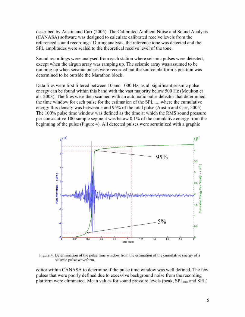
Data files were first filtered between 10 and 1000 Hz, as all significant seismic pulse energy can be found within this band with the vast majority below 500 Hz (Moulton et al., 2003). The files were then scanned with an automatic pulse detector that determined the time window for each pulse for the estimation of the SPLrms, where the cumulative energy flux density was between 5 and 95% of the total pulse (Austin and Carr, 2005). The 100% pulse time window was defined as the time at which the RMS sound pressure per consecutive 100-sample segment was below 0.1% of the cumulative energy from the beginning of the pulse (Figure 4). All detected pulses were scrutinized with a graphic

editor within CANASA to determine if the pulse time window was well defined. The few pulses that were poorly defined due to excessive background noise from the recording platform were eliminated. Mean values for sound pressure levels (peak, SPLrms and SEL)

95%

5%

Figure 4. Determination of the pulse time window from the estimation of the cumulative energy of a seismic pulse waveform.

6

were estimated for each station by averaging (linear scale) over all remaining pulses (20 < n < 166 per station). Finally, selected stations were scrutinized to compare measured SPL results with model predictions from Moulton et al. (2003).

Sound Level: Spectral Analyses Fast Fourier Transforms (FFT) were used to examine the frequency content of the seismic pulses at various distances from the source. Sound levels (dB re 1µPa) were measured at 1/6 octave bands (toothed whale critical band) starting at 10 Hz (central frequency) to produced 3D noise spectrograms. These sound spectra were compared to a toothed whale’s audiogram to determine audibility. Although the northern bottlenose whale was the species of most concern, the only large odontocete audiogram available to us was from the beluga whale, Delphinapterus leucas (Erbe and Farmer, 2000). We assumed that the beluga whale audiogram would represent the upper limit of the hearing sensitivity of the northern bottlenose whale given that, in general, larger marine mammals exhibit higher sensitivity at lower frequencies. Therefore, comparison of the seismic sound levels with the beluga whale audiogram should be a conservative approximation to what a northern bottlenose whale should be able to hear at low frequencies (< 500 Hz).

Ambient Noise For the ambient noise analyses, power spectral density (PSD) levels (dB re 1µPa2/Hz) were estimated using FFT analysis over the recorded bandwidth and presented in 1/3 octave bands for comparison with published measurements. Files were first scrutinized with a sound file editor (CoolEdit, Syntrillium ®) to identify, select and eliminate platform-related noise. Noise was considered PRN either audibly or if it appeared to be related to wave movements, such as metallic thumping. This was particularly obvious for the shallower stations.

RESULTS

SURVEY COVERAGE AND SYSTEM PERFORMANCE

Rough weather prevented sampling at 12 of the 24 planned stations during the April survey. Also, significant PRN was noted on most recordings, making the estimation of ambient noise levels difficult for those stations. Therefore, only the cleanest data were analysed. From the July survey, all stations were visited at least once and seismic pulses were recorded at all stations except D3, as the airguns were off during both visits.

PULSE CHARACTERISTICS

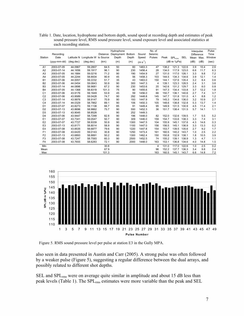
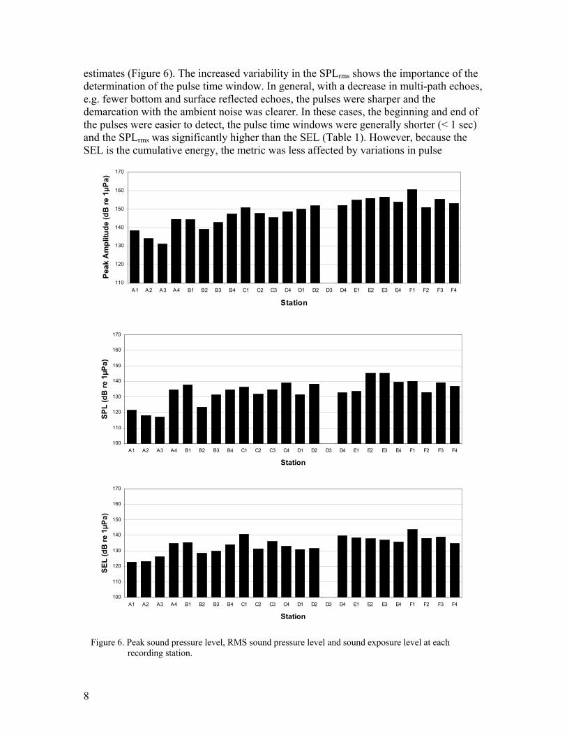
The highest average peak, SPLrms and SEL amplitudes per station were 161 (station F1), 145 (stations E2, E3) and 144 (station F1) dB re 1µPa, respectively, during the period of our field measurements (Table 1). Pulse amplitude variability over the 0.5 h recordings was considerable both within and among stations, partially due to variable range and propagation conditions from the displacement of the source vessel, but also due to differences between the alternating arrays. The mean SPLrms inter-pulse difference varied from 1 to 6 dB from station to station (Table 1). Variability of this magnitude was

7

also seen in data presented in Austin and Carr (2005). A strong pulse was often followed by a weaker pulse (Figure 5), suggesting a regular difference between the dual arrays, and possibly related to different shot depths.

SEL and SPLrms were on average quite similar in amplitude and about 15 dB less than peak levels (Table 1). The SPLrms estimates were more variable than the peak and SEL

110115120125130135140145150155160

1 3 5 7 9 11 13 15 17 19 21 23 25 27 29 31 33 35 37 39 41 43 45 47 49Pulse Numbe r

SPL

(dB

re 1

µPa)

Figure 5. RMS sound pressure level per pulse at station E3 in the Gully MPA.

Table 1. Date, location, hydrophone and bottom depth, sound speed at recording depth and estimates of peak sound pressure level, RMS sound pressure level, sound exposure level and associated statistics at each recording station.

StationRecording

Date Latitude N Longitude WDistance to Source

Hydrophone Deployment

DepthBottom Depth

Sound Speed

No. of Seismic Pulses Peak SPLrms SEL

Pulse Time

Window(yyyy-mm-dd) (deg.dec) (deg.dec) (km) (m) (m) (m·s-1) (dB) (dB) (sec)

A1 2003-07-05 44.0967 59.2807 64.5 50 60 1463.3 47 138.2 121.3 122.6 3.9 10.4 2.6A2 2003-07-14 44.1656 59.1917 96.1 90 230 1456.4 28 134.0 117.9 123.0 6.6 11.7 6.3A3 2003-07-05 44.1884 59.0216 71.2 90 190 1454.9 27 131.0 117.0 126.1 3.3 9.8 7.2A4 2003-07-05 44.2244 58.8934 90.9 45 56 1458.3 103 144.5 134.3 134.6 3.9 12.1 1.4B1 2003-07-06 44.0057 59.2232 51.7 35 43 1463.0 150 144.1 137.6 135.4 3.2 8.4 0.6B2 2003-07-06 44.0454 59.0843 50.9 90 300 1447.3 4 139.1 123.3 128.5 2.4 3.1 3.6B3 2003-07-14 44.0896 58.9681 67.2 90 230 1453.6 20 142.6 131.2 129.7 3.3 8.0 0.8B4 2003-07-05 44.1368 58.8318 101.3 75 90 1455.6 91 147.3 134.4 133.8 3.7 12.2 1.8C1 2003-07-06 43.9176 59.1649 53.9 45 59 1456.0 66 150.7 136.1 140.6 2.7 7.4 3.7C2 2003-07-06 43.9589 59.0428 74.7 90 292 1448.8 145 147.7 131.8 131.0 4.1 8.8 1.2C3 2003-07-14 43.9976 58.9147 70.9 90 193 1447.9 79 145.3 134.6 136.0 3.2 10.9 2.7C4 2003-07-14 44.0329 58.7862 89.1 90 106 1450.3 105 148.6 138.8 132.8 5.3 13.7 1.4D1 2003-07-07 43.8273 59.1138 66.7 85 91 1449.4 95 149.9 131.5 130.9 4.5 11.4 2.1D2 2003-07-13 43.8696 58.9862 75.7 90 550 1452.3 36 151.7 138.4 131.5 5.7 14.1 1.1D3 2003-07-13 43.9045 58.8528 90 252 1449.3D4 2003-07-06 43.9447 58.7299 82.8 90 196 1448.0 82 152.0 132.6 139.5 1.7 5.5 5.2E1 2003-07-07 43.7341 59.0547 50.7 90 309 1446.0 159 154.7 133.6 138.3 3.3 7.4 3.1E2 2003-07-07 43.7727 58.9339 50.9 90 1300 1447.5 104 155.9 145.1 137.6 4.3 14.6 0.3E3 2003-07-13 43.8171 58.8014 58.9 90 1100 1447.0 156 156.5 145.1 136.9 3.3 13.3 0.2E4 2003-07-08 43.8535 58.6877 79.6 90 1220 1447.8 154 153.7 139.5 135.6 2.7 9.2 1.7F1 2003-07-08 43.6420 59.0143 30.8 90 1250 1473.4 161 160.5 140.2 143.7 1.0 2.5 2.2F2 2003-07-13 43.6893 58.8891 50.2 90 1300 1462.4 150 150.8 132.9 138.1 1.8 10.5 3.9F3 2003-07-08 43.7247 58.7593 60.3 90 2500 1452.5 74 155.2 139.1 138.9 1.3 4.7 1.1F4 2003-07-08 43.7655 58.6283 72.1 90 2000 1448.0 163 153.1 136.8 134.6 4.0 14.8 1.5Min 30.8 4 131.0 117.0 122.6 1.0 2.5 0.2

Mean 67.9 96 152.2 137.7 136.3 3.4 9.8 2.4Max 101.3 163 160.5 145.1 143.7 6.6 14.8 7.2

(dB re 1µPa)

Interpulse Difference

Mean Max.

8

estimates (Figure 6). The increased variability in the SPLrms shows the importance of the determination of the pulse time window. In general, with a decrease in multi-path echoes, e.g. fewer bottom and surface reflected echoes, the pulses were sharper and the demarcation with the ambient noise was clearer. In these cases, the beginning and end of the pulses were easier to detect, the pulse time windows were generally shorter (< 1 sec) and the SPLrms was significantly higher than the SEL (Table 1). However, because the SEL is the cumulative energy, the metric was less affected by variations in pulse

110

120

130

140

150

160

170

A1 A2 A3 A4 B1 B2 B3 B4 C1 C2 C3 C4 D1 D2 D3 D4 E1 E2 E3 E4 F1 F2 F3 F4

Station

Peak

Am

plitu

de (d

B re

1µP

a)

100

110

120

130

140

150

160

170

A1 A2 A3 A4 B1 B2 B3 B4 C1 C2 C3 C4 D1 D2 D3 D4 E1 E2 E3 E4 F1 F2 F3 F4

Station

SPL

(dB

re 1

µPa)

100

110

120

130

140

150

160

170

A1 A2 A3 A4 B1 B2 B3 B4 C1 C2 C3 C4 D1 D2 D3 D4 E1 E2 E3 E4 F1 F2 F3 F4

Station

SEL

(dB

re 1

µPa)

Figure 6. Peak sound pressure level, RMS sound pressure level and sound exposure level at each recording station.

9

windows detection, since the tail ends of the pulses contained relatively little energy, resulting in higher measurement stability.

PROPAGATION

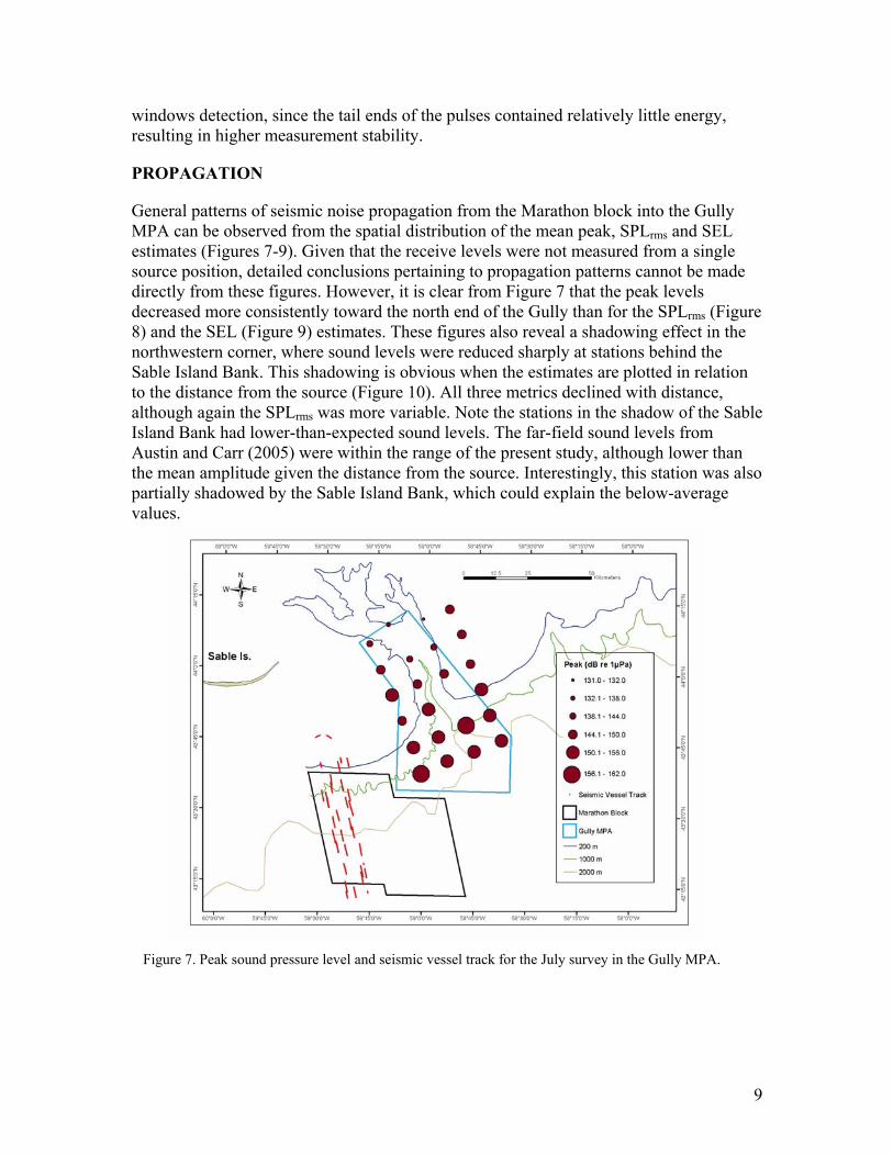
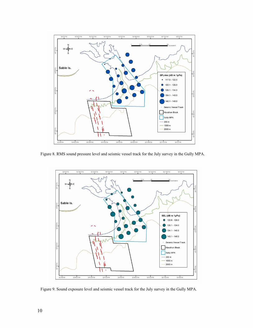
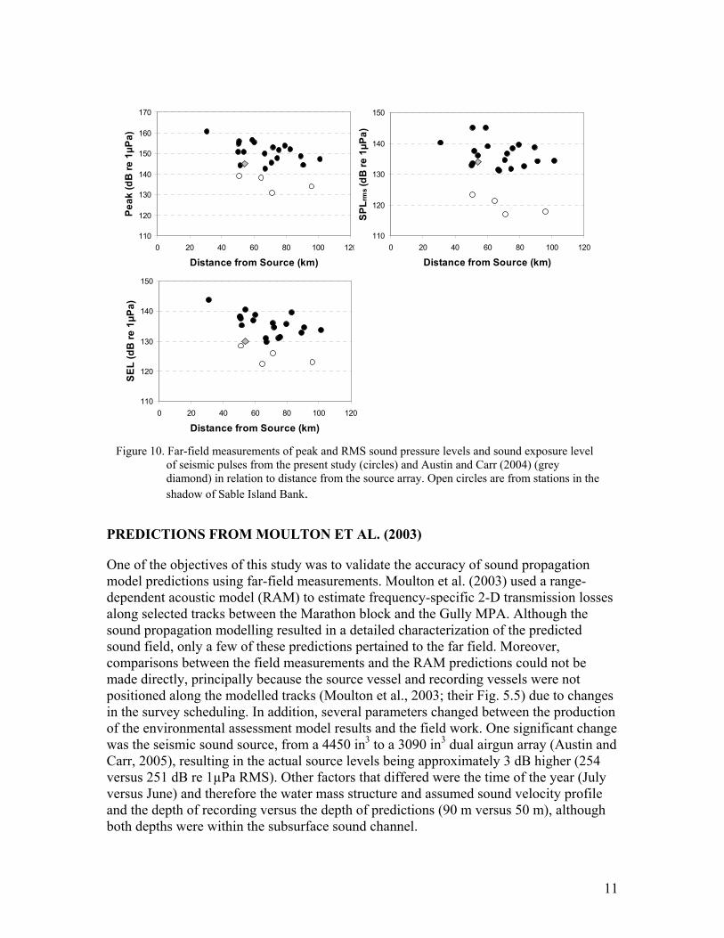
General patterns of seismic noise propagation from the Marathon block into the Gully MPA can be observed from the spatial distribution of the mean peak, SPLrms and SEL estimates (Figures 7-9). Given that the receive levels were not measured from a single source position, detailed conclusions pertaining to propagation patterns cannot be made directly from these figures. However, it is clear from Figure 7 that the peak levels decreased more consistently toward the north end of the Gully than for the SPLrms (Figure 8) and the SEL (Figure 9) estimates. These figures also reveal a shadowing effect in the northwestern corner, where sound levels were reduced sharply at stations behind the Sable Island Bank. This shadowing is obvious when the estimates are plotted in relation to the distance from the source (Figure 10). All three metrics declined with distance, although again the SPLrms was more variable. Note the stations in the shadow of the Sable Island Bank had lower-than-expected sound levels. The far-field sound levels from Austin and Carr (2005) were within the range of the present study, although lower than the mean amplitude given the distance from the source. Interestingly, this station was also partially shadowed by the Sable Island Bank, which could explain the below-average values.

Figure 7. Peak sound pressure level and seismic vessel track for the July survey in the Gully MPA.

10

Figure 9. Sound exposure level and seismic vessel track for the July survey in the Gully MPA.

Figure 8. RMS sound pressure level and seismic vessel track for the July survey in the Gully MPA.

11

PREDICTIONS FROM MOULTON ET AL. (2003)

One of the objectives of this study was to validate the accuracy of sound propagation model predictions using far-field measurements. Moulton et al. (2003) used a range-dependent acoustic model (RAM) to estimate frequency-specific 2-D transmission losses along selected tracks between the Marathon block and the Gully MPA. Although the sound propagation modelling resulted in a detailed characterization of the predicted sound field, only a few of these predictions pertained to the far field. Moreover, comparisons between the field measurements and the RAM predictions could not be made directly, principally because the source vessel and recording vessels were not positioned along the modelled tracks (Moulton et al., 2003; their Fig. 5.5) due to changes in the survey scheduling. In addition, several parameters changed between the production of the environmental assessment model results and the field work. One significant change was the seismic sound source, from a 4450 in3 to a 3090 in3 dual airgun array (Austin and Carr, 2005), resulting in the actual source levels being approximately 3 dB higher (254 versus 251 dB re 1µPa RMS). Other factors that differed were the time of the year (July versus June) and therefore the water mass structure and assumed sound velocity profile and the depth of recording versus the depth of predictions (90 m versus 50 m), although both depths were within the subsurface sound channel.

110

120

130

140

150

0 20 40 60 80 100 120

Distance from Source (km)

SEL

(dB

re 1

µPa)

110

120

130

140

150

160

170

0 20 40 60 80 100 120

Distance from Source (km)

Peak

(dB

re 1

µPa)

110

120

130

140

150

0 20 40 60 80 100 120

Distance from Source (km)

SPL r

ms (

dB re

1µP

a)

Figure 10. Far-field measurements of peak and RMS sound pressure levels and sound exposure level of seismic pulses from the present study (circles) and Austin and Carr (2004) (grey diamond) in relation to distance from the source array. Open circles are from stations in the shadow of Sable Island Bank.

12

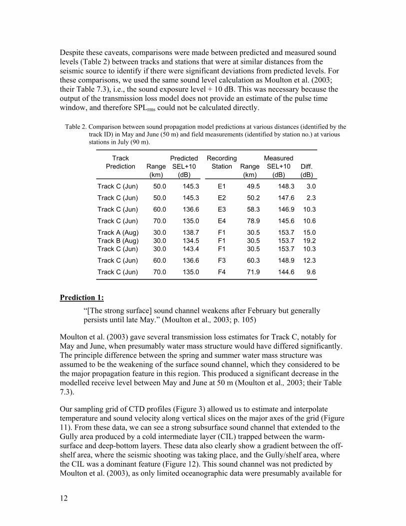
Despite these caveats, comparisons were made between predicted and measured sound levels (Table 2) between tracks and stations that were at similar distances from the seismic source to identify if there were significant deviations from predicted levels. For these comparisons, we used the same sound level calculation as Moulton et al. (2003; their Table 7.3), i.e., the sound exposure level + 10 dB. This was necessary because the output of the transmission loss model does not provide an estimate of the pulse time window, and therefore SPLrms could not be calculated directly.

Prediction 1: “[The strong surface] sound channel weakens after February but generally persists until late May.” (Moulton et al., 2003; p. 105)

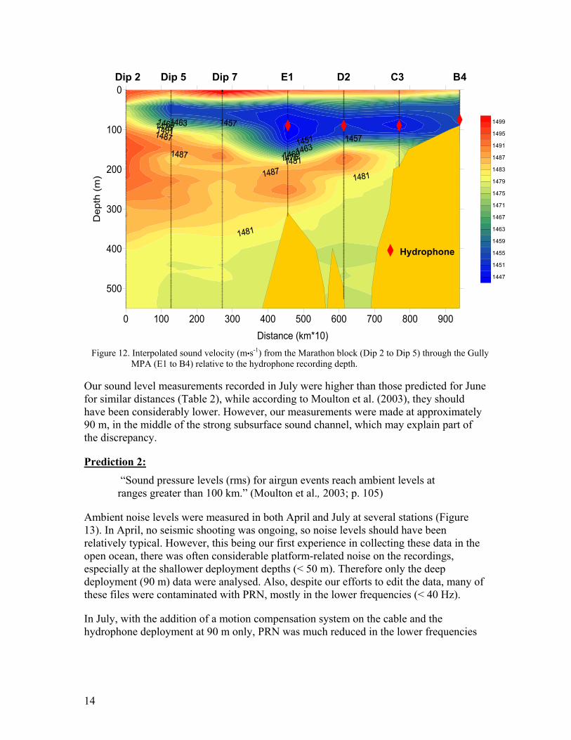
Moulton et al. (2003) gave several transmission loss estimates for Track C, notably for May and June, when presumably water mass structure would have differed significantly. The principle difference between the spring and summer water mass structure was assumed to be the weakening of the surface sound channel, which they considered to be the major propagation feature in this region. This produced a significant decrease in the modelled receive level between May and June at 50 m (Moulton et al., 2003; their Table 7.3).

Our sampling grid of CTD profiles (Figure 3) allowed us to estimate and interpolate temperature and sound velocity along vertical slices on the major axes of the grid (Figure 11). From these data, we can see a strong subsurface sound channel that extended to the Gully area produced by a cold intermediate layer (CIL) trapped between the warm-surface and deep-bottom layers. These data also clearly show a gradient between the off-shelf area, where the seismic shooting was taking place, and the Gully/shelf area, where the CIL was a dominant feature (Figure 12). This sound channel was not predicted by Moulton et al. (2003), as only limited oceanographic data were presumably available for

Table 2. Comparison between sound propagation model predictions at various distances (identified by the track ID) in May and June (50 m) and field measurements (identified by station no.) at various stations in July (90 m).

Track Prediction Range

Recording Station Range

Measured SEL+10

(km) (km) (dB)

Track C (Jun) 50.0 145.3 E1 49.5 148.3 3.0

Track C (Jun) 50.0 145.3 E2 50.2 147.6 2.3

Track C (Jun) 60.0 136.6 E3 58.3 146.9 10.3

Track C (Jun) 70.0 135.0 E4 78.9 145.6 10.6

Track A (Aug) 30.0 138.7 F1 30.5 153.7 15.0Track B (Aug) 30.0 134.5 F1 30.5 153.7 19.2Track C (Jun) 30.0 143.4 F1 30.5 153.7 10.3

Track C (Jun) 60.0 136.6 F3 60.3 148.9 12.3

Track C (Jun) 70.0 135.0 F4 71.9 144.6 9.6

Predicted SEL+10 Diff.

(dB) (dB)

13

this area at the time of the model runs. Therefore, using sound velocity profiles from the offshore as input into the RAM for predicting transmission losses into the Gully MPA could significantly bias predicted transmission losses.

1 2

3 4

Figure 11. Interpolated sound velocity (m•s-1) along transect lines (1) A1-F1, (2) A2-F2, (3) A3-F3 and (4) A4-F4 (see Figure 3) within the Gully MPA. Black lines indicate profile positions.

14

Our sound level measurements recorded in July were higher than those predicted for June for similar distances (Table 2), while according to Moulton et al. (2003), they should have been considerably lower. However, our measurements were made at approximately 90 m, in the middle of the strong subsurface sound channel, which may explain part of the discrepancy.

Prediction 2:

“Sound pressure levels (rms) for airgun events reach ambient levels at ranges greater than 100 km.” (Moulton et al., 2003; p. 105)

Ambient noise levels were measured in both April and July at several stations (Figure 13). In April, no seismic shooting was ongoing, so noise levels should have been relatively typical. However, this being our first experience in collecting these data in the open ocean, there was often considerable platform-related noise on the recordings, especially at the shallower deployment depths (< 50 m). Therefore only the deep deployment (90 m) data were analysed. Also, despite our efforts to edit the data, many of these files were contaminated with PRN, mostly in the lower frequencies (< 40 Hz).

In July, with the addition of a motion compensation system on the cable and the hydrophone deployment at 90 m only, PRN was much reduced in the lower frequencies

0 100 200 300 400 500 600 700 800 900Distance (km*10)

500

400

300

200

100

0D

epth

(m

)

1447

1451

1455

1459

1463

1467

1471

1475

1479

1483

1487

1491

1495

1499

Dip 2 Dip 5 Dip 7 E1 D2 C3 B4

Hydrophone

Figure 12. Interpolated sound velocity (m•s-1) from the Marathon block (Dip 2 to Dip 5) through the Gully MPA (E1 to B4) relative to the hydrophone recording depth.

15

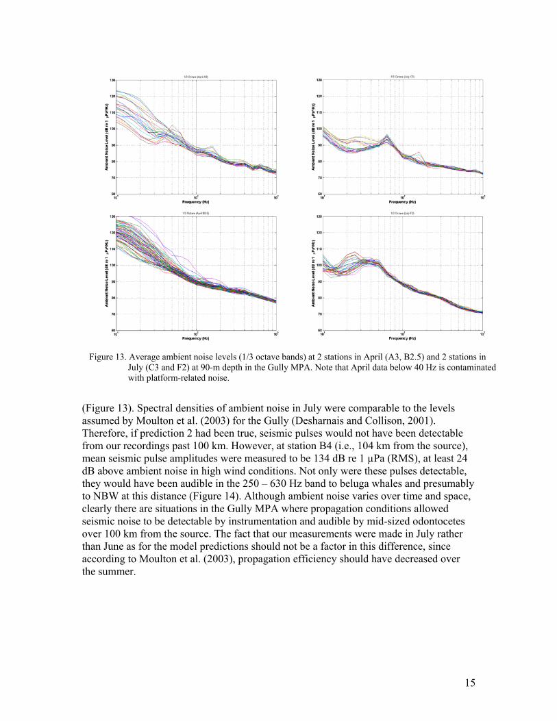
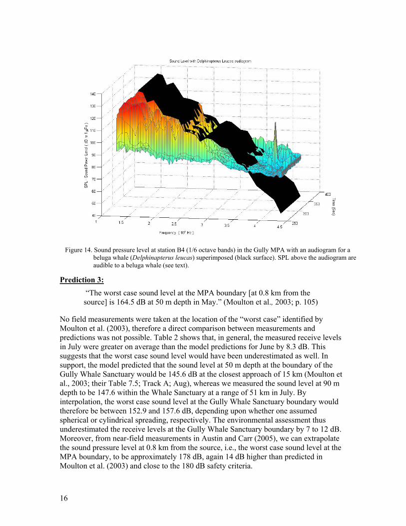
(Figure 13). Spectral densities of ambient noise in July were comparable to the levels assumed by Moulton et al. (2003) for the Gully (Desharnais and Collison, 2001). Therefore, if prediction 2 had been true, seismic pulses would not have been detectable from our recordings past 100 km. However, at station B4 (i.e., 104 km from the source), mean seismic pulse amplitudes were measured to be 134 dB re 1 µPa (RMS), at least 24 dB above ambient noise in high wind conditions. Not only were these pulses detectable, they would have been audible in the 250 – 630 Hz band to beluga whales and presumably to NBW at this distance (Figure 14). Although ambient noise varies over time and space, clearly there are situations in the Gully MPA where propagation conditions allowed seismic noise to be detectable by instrumentation and audible by mid-sized odontocetes over 100 km from the source. The fact that our measurements were made in July rather than June as for the model predictions should not be a factor in this difference, since according to Moulton et al. (2003), propagation efficiency should have decreased over the summer.

Figure 13. Average ambient noise levels (1/3 octave bands) at 2 stations in April (A3, B2.5) and 2 stations in July (C3 and F2) at 90-m depth in the Gully MPA. Note that April data below 40 Hz is contaminated with platform-related noise.

16

Prediction 3: “The worst case sound level at the MPA boundary [at 0.8 km from the source] is 164.5 dB at 50 m depth in May.” (Moulton et al., 2003; p. 105)

No field measurements were taken at the location of the “worst case” identified by Moulton et al. (2003), therefore a direct comparison between measurements and predictions was not possible. Table 2 shows that, in general, the measured receive levels in July were greater on average than the model predictions for June by 8.3 dB. This suggests that the worst case sound level would have been underestimated as well. In support, the model predicted that the sound level at 50 m depth at the boundary of the Gully Whale Sanctuary would be 145.6 dB at the closest approach of 15 km (Moulton et al., 2003; their Table 7.5; Track A; Aug), whereas we measured the sound level at 90 m depth to be 147.6 within the Whale Sanctuary at a range of 51 km in July. By interpolation, the worst case sound level at the Gully Whale Sanctuary boundary would therefore be between 152.9 and 157.6 dB, depending upon whether one assumed spherical or cylindrical spreading, respectively. The environmental assessment thus underestimated the receive levels at the Gully Whale Sanctuary boundary by 7 to 12 dB. Moreover, from near-field measurements in Austin and Carr (2005), we can extrapolate the sound pressure level at 0.8 km from the source, i.e., the worst case sound level at the MPA boundary, to be approximately 178 dB, again 14 dB higher than predicted in Moulton et al. (2003) and close to the 180 dB safety criteria.

Figure 14. Sound pressure level at station B4 (1/6 octave bands) in the Gully MPA with an audiogram for a

beluga whale (Delphinapterus leucas) superimposed (black surface). SPL above the audiogram are audible to a beluga whale (see text).

17

The field measurements in Table 2 represent approximations of RMS sound pressure levels, averaged over many pulses. There was nonetheless significant variability around these average values (Table 1; Figure 5). Some of this variability was from pulse to pulse, and some was over the period of the recording. Therefore, not only were average measured sound levels greater than estimated levels, individual pulses were several dB higher than these averages.

Deviations in pulse amplitude over the time of the recordings should not strictly have been due to the effects of distance since the range of distances between source and reception for a given station was 0 – 5% of the total distance due to the displacement of the source vessel. The maximum SPL was often 5 dB above the mean and on occasion as much as 9 dB higher. Therefore, it is not necessarily true that the average sound level predicted by the RAM at the closest point to the Gully MPA can be interpreted as the “worst case sound level”. Individual pulses can be significantly higher than the average.

DISCUSSION

The systematic sampling grid allowed us to produce an overall picture of the noise field within the Gully MPA, both ambient and that generated by airgun array pulses from a nearby 3-D seismic survey. The rescheduling of the survey did not allow us to take field measurements from positions identical to the published RAM predictions, nor at the closest point of approach to the Gully MPA; however, several recordings were made at similar distances from the source as those that were modelled.

Our results showed that the predictions from Moulton et al. (2003) were on average underestimated by 8 dB. This finding is significant since the results of sound propagation models are used by regulators to define the safety radius for marine mammals around seismic arrays. The field validation conducted during this and other studies as part of the Gully Seismic Research Program provided the means to monitor the sound levels and to observe that these sound levels were higher than expected. In fact, the near-field measurements reported in Austin and Carr (2005) were used to expand the safety radius from 500 to 700 m during operations.

Transmission loss models are important tools for indicating expected sound propagation patterns from a sound source such as a seismic array. However, these models are highly dependent on the accuracy and detail of the assumptions and environmental parameters put into them, including bathymetric, topographic, geoacoustic and oceanographic information (McCammon et al., 2005). For example, Moulton et al. (2003) assumed that propagation efficiency would degrade over the summer with the disappearance of the surface sound channel, while measurements taken by us and Austin and Carr (2005) showed that propagation conditions in July were as good as or better than those estimated for June. The strong subsurface sound channel formed by the CIL was not input into the RAM and may have resulted in the underestimation of the predicted levels. Austin and Carr (2005) demonstrated that field measurements and model estimates can show good agreement, although for their comparison the RAM transmission losses were remodelled with oceanographic data taken during the seismic survey and source levels from the array actually used. They also presented data indicating large discrepancies (up to 10 dB)

18

between estimated and measured sound levels for particular frequency bands and locations, indicating that some local environmental variability was not captured in the model. Our data showed that the specific characteristics of the regional sound propagation, such as the shadowing produced by the Sable Island Bank, can significantly affect expected sound levels. This underlines the importance of conducting extensive field validation under a variety of conditions.

There is also a need to have some measure of the variability around the model estimates. Deterministic transmission loss models provide no indication of uncertainty and must be used with caution. Sources of uncertainty will not only include the variable and possibly inaccurate physical parameters in the propagation model but will also include pulse-to-pulse variation of the seismic array. To avoid exposing animals to higher-than-expected energy pulses, a wide buffer should be added to the estimated safety zone to reflect the margin of error. The present study has shown that errors on the order of 10 dB or more are not unusual.

Although SPLrms is the most common unit used to compare sound levels between studies, this metric varies considerably depending on the width of the estimated pulse time window and can be considerably underestimated. This point is well illustrated by the major differences between SPLrms and peak sound levels (Table 1). In the present study, the mean peak level was 15 dB higher than the mean SPLrms and SEL. This gap was in part due to the difficulty in defining the RMS time window, since many of the pulses were drawn out in time, thereby reducing the SPLrms estimate. Our analyses showed that the inter-pulse variation in SPLrms could be as high as 10 dB over many stations. When pulses were clearly defined, i.e., with few multi-path echoes, such as for stations E2 and E3, the SPL estimates were clearly higher, and the difference between the peak, SPL and SEL was approximately 10 dB each, as discussed by Malme et al. (1984). This suggests that the mean SPLrms is not the best metric for the description of the received level of pulsed sounds.

CONCLUSIONS

From this study, several conclusions can be drawn:

• The highest average sound pressure level (RMS) measured in the Gully MPA was 145 dB re 1µPa at 90 m depth, 50 km from the seismic array. This sound level was measured within the Gully Whale Sanctuary while the seismic vessel was surveying the western portion of the exploration block. It was estimated that sound levels in the Whale Sanctuary would have been higher, between approximately 153 and 157 dB, when the vessel was at its closest approach to the Gully in the eastern portion of the survey block. The “worst case” sound level at the Gully MPA boundary, i.e., 0.8 km from the source, can be estimated from the extrapolation of near-field measurements in Austin and Carr (2005) to be approximately 178 dB, 14 dB higher than predicted in Moulton et al. (2003).

• Models predict average conditions and do not capture the spatial and temporal variability of the real environment. Measured sound levels were significantly higher

19

than the model predictions at several stations. In addition, the range of audibility of seismic pulses to a mid-sized odontocete similar to a northern bottlenose whale was significantly underestimated relative to the model predictions. This demonstrates the importance of using accurate model input data, the importance of field validation and the need to have a measure of the variability around the mean sound level estimates. Transmission losses should be re-modelled if actual field conditions differ from assumptions.

• Sound pressure levels (RMS) varied considerably in relation to the width of the estimated pulse time window, which was dependent on the magnitude of multi-path arrivals. Although SPLrms is the standard measurement for comparison to safety limit criteria for marine mammals, it is not a good metric for the description of pulsed sounds due to the inconsistency of the pulse time window.

ACKNOWLEDGEMENTS

The authors wish to thank Jean-François Gosselin, Patrick Abgrall, Jack Lawson, Pierre Carter, Steven Benjamins and crew members of the Strait Signet for their tireless efforts during data collection, and Samuel Lambert-Milot and Amélie Robillard for their assistance in the data analyses. We also wish to thank Yves Samson and Sylvain Chartrand of the Hydroacoustic Laboratory (MLI), who conceived and built the RUSTLER system and executed several rapid modifications to prepare for these surveys. We also wish to thank the six external referees for their valuable comments. Funding for this study was provided through the DFO Center of Offshore Oil and Gas Environmental Research (COOGER).

REFERENCES

Austin, M.E. and Carr, S.A. 2005. Summary report on acoustic monitoring of Marathon Canada Petroleum ULC 2003 Cortland/Empire 3-D seismic program. Environmental Studies Research Funds series: 17 p. Available from the Maurice Lamontagne Institute Library, Department of Fisheries and Oceans, Mont-Joli, Qc, G5H 3Z4, Canada.

Desharnais, F. and Collison, N. 2001. An assessment of the noise field near the Sable Gully area. Proceedings of Oceans 2001 Conference, Honolulu, HI, 3: 1348-1355.

Erbe, C. and Farmer, D. 2000. Zones of impact around icebreakers affecting beluga whales in the Beaufort Sea. Journal of Acoustical Society of America, 108(3): 1332-1340.

Malme, C., Miles, P., Clark, C., Tyack, P. and Bird, J. 1984. Investigations of the potential effects of underwater noise from petroleum industry activities on migrating gray whale behavior / Phase II: January 1984 migration, BBN Rep. 5586. Rep. from Bolt Beranek and Newman Inc., Cambridge, MA, for U.S. Minerals Management Service, Anchorage, AK.

McCammon, D., Racca, R., Austin, M., Laurinolli, M. and Carr S. 2005. Applicability of sound propagation models in the marine and freshwater environment, JASCO

20

Research. Available from the Maurice Lamontagne Institute Library, Department of Fisheries and Oceans, Mont-Joli, Qc, G5H 3Z4, Canada.

Moulton, V., Davis, R., Cook, J., Austin, M., Reece, M., Martin, S., MacGillivray, A., Hannay, D. and Fitzgerald, M. 2003. Environmental Assessment of Marathon Canada Limited’s 3-D Seismic Program on the Scotian Slope. LGL Report SA 744-1. Halifax, Nova Scotia.: 173. Available from the Maurice Lamontagne Institute Library, Department of Fisheries and Oceans, Mont-Joli, Qc, G5H 3Z4, Canada.

Whitehead, H., Gowans, S., Faucher, A. and McCarrey, S. W. 1997. Population analysis of northern bottlenose whales in the Gully, Nova Scotia. Marine Mammal Science, 13(2): 173-185.