Family Background, School Choice, and Students' Academic ...

Family Background, School Choice, and

Students' Academic Performance: Evidence from

Sri Lanka

Harsha Aturupane

Tomokazu Nomura

Mari Shojo

September 2018

Discussion Paper No.1811

GRADUATE SCHOOL OF ECONOMICS

KOBE UNIVERSITY

ROKKO, KOBE, JAPAN

1

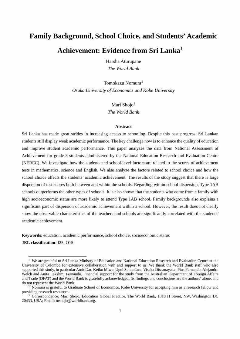
Family Background, School Choice, and Students’ Academic

Achievement: Evidence from Sri Lanka1 Harsha Aturupane The World Bank

Tomokazu Nomura2 Osaka University of Economics and Kobe University

Mari Shojo3 The World Bank

Abstract Sri Lanka has made great strides in increasing access to schooling. Despite this past progress, Sri Lankan students still display weak academic performance. The key challenge now is to enhance the quality of education and improve student academic performance. This paper analyzes the data from National Assessment of Achievement for grade 8 students administered by the National Education Research and Evaluation Centre (NEREC). We investigate how the student- and school-level factors are related to the scores of achievement tests in mathematics, science and English. We also analyze the factors related to school choice and how the school choice affects the students’ academic achievement. The results of the study suggest that there is large dispersion of test scores both between and within the schools. Regarding within-school dispersion, Type 1AB schools outperforms the other types of schools. It is also shown that the students who come from a family with high socioeconomic status are more likely to attend Type 1AB school. Family backgrounds also explains a significant part of dispersion of academic achievement within a school. However, the result does not clearly show the observable characteristics of the teachers and schools are significantly correlated with the students’ academic achievement.

Keywords: education, academic performance, school choice, socioeconomic status JEL classification: I25, O15

1 We are grateful to Sri Lanka Ministry of Education and National Education Research and Evaluation Centre at the University of Colombo for extensive collaboration with and support to us. We thank the World Bank staff who also supported this study, in particular Amit Dar, Keiko Miwa, Upul Sonnadara, Visaka Dissanayake, Pius Fernando, Alejandro Welch and Anita Lakshmi Fernando. Financial support for the study from the Australian Department of Foreign Affairs and Trade (DFAT) and the World Bank is gratefully acknowledged. Its findings and conclusions are the authors’ alone, and do not represent the World Bank.

2 Nomura is grateful to Graduate School of Economics, Kobe University for accepting him as a research fellow and providing research resources.

3 Correspondence: Mari Shojo, Education Global Practice, The World Bank, 1818 H Street, NW, Washington DC 20433, USA; Email: [email protected].

2

1 Introduction

Sri Lanka has made a great deal of effort to improve its education system and achieve education goals such as education Millennium Development Goals (MDGs). As a result, net primary school enrollment ratio has reached 99 percent, while the secondary school enrollment ratio also improved from 78 percent in 2006 to 84 percent in 2012. Gender parity is also high in primary and junior secondary education enrollment (World Bank 2015). Despite these achievements, however, some recent reports show that Sri Lankan students still display weak academic performance when compared to their international peers (World Bank 2012).

There is broad agreement, backed by international research findings, that education is a powerful driver of improved quality of skills, and is one of the significant instruments for increased individual earnings, labor productivity and economic growth. High-quality education (that is, fostering high learning achievement) enhances people’s ability to control their fertility rate and family health. It also facilitates gender equality, peace, and stability (World Bank 2011b; UNESCO 2014). However, recent studies suggest that the expansion of enrollment is not necessarily associated with the improvement of human capital quality in many developing countries (Hanushek and Woessmann, 2007, 2012).

It is common understanding that the cognitive skills measured by international achievement tests (e.g. PISA4 and TIMMS5) work as good proxies for the quality of human capital, and are the keys for the economic growth (E. A. Hanushek & Kimko, 2000). Thus, the nature of quality of education and its association with good learning outcomes have been of great interest to educators and researchers in recent decades.

Learning is a product of the combination of formal schooling and factors related to students’ families, communities, and peers (Rothstein 2000). Numerous attempts have been made by researchers to investigate the determinants of student achievement; however, consensus has yet to be achieved concerning factors influencing student academic performance, and the findings of these numerous studies are mixed and inconclusive. For instance, Coleman et al. (1966) asserted the importance of family characteristics to explain variation in student achievement and the relatively small impact of school-level characteristics on student achievement. This “Coleman Report” generated a flurry of research and debate on student achievement. Based on data from both developed and developing countries, Heyneman and Loxley (1983) concluded that in low income countries, the impact of school characteristics on student achievement is comparatively greater than in higher income countries.

Student-level characteristics that have been identified in the literature as potentially contributing to difference in student achievement include gender, socioeconomic status, family size, parental education level, attendance at private lessons/tuition, self-confidence, presence of books at home, and doing homework at home. School-level characteristics such as school resources, school type, location, class size, teachers’ years of experience, and teachers’ training were also found to influence student achievement. While some research has shown that both student- and school-level factors have a strong impact on student performance, some studies have found further that some specific factors have less impact or a negative impact (for literature review, see

4 Programme for International Student Assessment. 5 Trends in International Mathematics and Science Study.

3

for instance, Hanushek 1995; Glewwe et al. 2011). Debates continue regarding factors influencing student performance in general.

There has been only few studies which examined factors associated with the learning achievements of Sri Lankan students so far. Aturupane et al. (2013), investigating the determinants of academic performance as measured by achievement tests conducted in 2004 for grade 4 students, claimed that among student-level variables, educated parents, better nutrition, frequent attendance, enrollment in private tutoring classes, access to exercise books, electric lighting at home, and children’s books at home positively influence the academic performance of the students. Among school-level variables, principals’ and teachers’ years of experience, collaboration with other schools in a “school family,” and frequent meetings between parents and teachers have positive impacts on the test scores. However, since then there has been no analysis of the determinants of students’ performance in Sri Lanka.

In the present study, we examine the determinants of academic performance among grade 8 students using recent data from the Sri Lankan National Assessment of Achievement conducted in 2012. This was the first assessment that used new instruments to test students’ cognitive skills in ways keeping with the new curriculum and the only one in recent years which collected detailed information on characteristics of students, their families, classrooms, teachers, principals, and schools in general. The 2012 National Assessment was intended to serve as a baseline for monitoring the level and distribution of learning outcomes over time. The findings have wide implications for future programs and policies to enhance the quality of education and improve learning outcomes in Sri Lanka.

This paper investigates student and school factors affecting learning outcomes for Mathematics, Science and English represented by the scores of achievement test among grade 8 students (aged 12-13) in Sri Lanka. It also analyzes the factors related to school choice and how the school choice affects the students’ performance. It contributes unique and important information to understanding these factors, as it is still unclear what characteristics of students and schools affect student performance at the secondary education in Sri Lanka.

The reminder of this paper is organized as follows. Section 2 provides general information about public education in Sri Lanka. Section 3 describes the data we use in the empirical analysis and presents the descriptive features of the test score distributions. Section 4 examines the relation between students’ family background and school choice, and estimates the treatment effects of attending a Type 1AB school (see Section 2 for school type) on learning outcomes. Section 5 analyzes the association between characteristics of students, and schools and students’ test scores. Section 6 discusses the nature and implications of the relations between the student/teacher/school characteristics and the test scores and concludes the paper.

2 The education system in Sri Lanka

After the end of a long period of civil conflict in 2009 with the government’s defeat of the Liberation Tigers of Tamil Eelam (LTTE) and with Sri Lanka’s concurrent overcoming of the effects global recession that began in 2008, the national economy has grown at an average of over 7 percent annually over the past several years.

4

The country is now classified as a lower middle income country, with per capita gross national income (GNI) of US$3,550 in 2015, and outperformed nearby country comparators on most of the 2015 MDGs; in general, human development indicators are impressive by regional and lower middle income standards.

The education system in Sri Lanka is organized into three cycles: primary education (grades 1–5), junior secondary education (grades 6–9), and senior secondary education (grades 10–13). Primary schooling commences at age 5 or 6 years. The net enrollment rate in primary education for both boys and girls is 99 percent, and at junior secondary level, 85 percent for boys and 84 percent for girls. There is thus a high degree of gender parity at these levels, which, however, declines somewhat at senior secondary level, with 67 percent of boys and 72 percent of girls.6

The government (public) school system in Sri Lanka is well developed and widely accessible around the county. Private schools are rare, accounting for less than 5 percent of total enrollment. Government schools are classified into four functional types that cover different grades and offer different curriculum streams: Type 1AB, Type 1C, Type 2, and Type 3: (a) Type 1AB schools (9 percent of total), which either cover the full primary and secondary cycle (grades 1–13) or secondary education alone (grades 6–13) and offer all three curriculum streams for the General Certificate of Examination Advanced Level (GCE A/L) courses (arts, commerce, and science); (b) Type 1C schools (19 percent of total), which also span grades 1–13 or 6–13 but offer only GCE A-level two streams (arts and commerce); (c) Type 2 schools (37 percent of total ), which offer classes only up to grade 11 and prepare students for GCE O-level examinations; and (d) Type 3 schools (35 percent of total), which go up only to grade 5 or 8. While most 1AB schools are in cities and towns, Types 1C and 2 are mainly in semi-urban and rural areas and Type 3 are mostly in rural areas. Since 1985, some 1AB schools have been designated “National” schools, funded and administered by the national Ministry of Education. The rest are “Provincial” schools, run by provincial councils.

The Government announces criteria for grade 1 admissions every year. Parents/legal guardians who expect to admit their children to grade one in schools should forward the relevant applications to the principals of schools. Applications could be made to more than one school. When the number of applicants received exceeds the number of students that could be accommodated in a certain school, the students will be called for an interview. Although admission to grade 1 is based, in principle, on residence, there is other marking criteria (e.g. children of parents who are past pupils of the school, siblings of students already studying in the school).

At the end of primary education, the majority of children sit the grade 5 scholarship examination, which was originally intended to be a basis for allocation of financial support for able but poor students and to facilitate access to high-quality schools for them. The scholarship examination is supposed to widen the school choice of students and increases the competition. Some research, however, indicates that the examination is now predominantly used by parents as a tool to gain entry for their children into popular national schools in urban areas (e.g., Little, Aturupane and Shojo 2013).

6 There are a few possible explanations for the lower survival rates for boys than for girls. First, some boys drop out of school and take up various jobs involving physical labor (World Bank 2011a). Another reason could be that some households appear to invest additional resources in girls’ education (Himaz 2010).

5

There are several demand- and supply-side policies in effect in Sri Lanka to promote school enrollment and attendance. Education is provided free of tuition costs in all government schools. Education up to grade 11 is compulsory, and all students from grades 1 to 11 receive free textbooks and uniforms. Students are entitled to subsidized transport in buses and trains. Free school meals are provided for primary students in disadvantaged areas. Supply-side policies complementing and supplementing the above-mentioned demand-side policies to promote participation and retention in schools include the existence of a comprehensive network of primary and secondary schools, with access to primary education available within two kilometers from home and to secondary education within five kilometers from home for all children. There is automatic progression through the education system up to grade 11. Special education programs are available for children with special education needs, and non-formal education programs are also available for adolescents who either never enrolled in school or dropped out at a young age (World Bank 2011a).

3 Data

This study uses the 2012 National Assessment of Achievement for grade 8 students, funded by the national Ministry of Education and administered by the National Education Research and Evaluation Centre (NEREC) at the University of Colombo. To assess the achievement level of students completing grade 8, NEREC constructed tests in mathematics, science and English based on the competency-based curriculum introduced nationwide in 2009. The National Assessment covered the entire country; a multi-stage sampling approach was used to enable analysis by province, type of school, student gender, and linguistic medium of instruction (Sinhala or Tamil). In the first stage, sample schools were selected within strata with probability proportional to size, without replacements. In the second stage, a group of students were selected from the sampled schools using a cluster sampling approach. In sample selection, the province was taken as the main stratum (explicit stratum). The final sample consisted of 12,821 grade 8 students in 438 public schools. In addition to the tests, information on characteristics of students, their families, classrooms, teachers, principals, and the schools in general was also collected through questionnaires administered to students, parents/guardians, teachers, and principals. Data collected through achievement tests were analyzed on a national and provincial basis, and were weighted in order to minimize the effect of the discrepancy between the expected and the achieved sample (NEREC 2013).

An overview of our dataset is presented in Tables 1 and 2. Table 1 shows representative statistics for test scores in mathematics, science, and English, while Table 2 provides descriptive statistics for the student variables, in panel (a), teacher and principal variables, in panel (b), and school characteristics, in panel (c). Test scores are measured out of 100 points. The outcome variables used for this study were student test scores in mathematics, science, and English. Based on both theoretical considerations and findings from previous empirical studies, several student- and school-level variables were selected to determine their associations with student learning achievement. At the student level, we include the gender of the student, number of siblings, distance from home to school, whether the student has an undisturbed learning environment at home, whether

6

the student uses English for communication at home, days absent from school over a two-month period, and time utilization for studying at home. We also include the family backgrounds of the students: educational attainment of the parents, family income, number of books available for the student to read at home, and tuition fees spent on the student. The school-level variables consist of characteristics of the teacher of each subject, the principal of the school, and the school as an institution. The information considered on the teachers includes gender, years of experience as a teacher, educational attainment, and whether they provide remedial teaching. The information on the principal includes gender, years of experience as a principal, and educational attainment. The school characteristics include location, school type, whether the school is managed by the national government or a provincial government, linguistic medium of instruction, index of school facilities7, number of students in the class, number of students in grade 8 in the school, proportion of students who have had their property stolen in the classroom, and proportion of students who have experienced violence in the classroom.

[Table 1 is inserted around here]


Before performing empirical analysis, we will present descriptive features of the test score distributions.

Figure 1 shows the estimated kernel densities of test scores, both for individual students and school averages, in each subject―mathematics, science, and English. Figure 1 considered together with Table 1 suggests that the academic performance of students in Sri Lanka as a whole is quite poor8. Mean scores are higher than the medians for all three subjects, and the distributions are considerably skewed to the right. The distributions of school average scores are similar in shape to the distributions of scores for individual students, suggesting that a substantial proportion of test score variance is due to variation between the schools.

[Figure 1 is inserted around here]

Among three focal subjects, achievement in English is particularly poor, with a mode of distribution of just a little over 20 points. Since the questions are mostly multiple-choice, this means that the majority of students achieved no more than the score that could be got by randomly choosing the answers. Mathematics and science show slightly better scores, which are also less skewed and show considerably higher densities in the right tails of the distributions.

7 The questionnaire for the principals includes a question about the availability of various school facilities and

materials (10 types of teaching aids, 5 additional facilities, and 21 physical facilities). Principals were asked to choose answers for each facility from the following options. 1: adequate in number and all in good condition and functioning; 2: adequate in number but not all in good condition/functioning; 3: not adequate and not all functioning; 4: not available. We constructed an index of school facilities for each school by counting facilities for which the principal chose 1 or 2.

8 Although the scores are not internationally comparable, the problems are standard and the scores can be considered as indicating the level of the understanding as proportions of required comprehension.

7

It is worth noting that the distributions of test scores show multiple modes, especially for mathematics and English. The distribution of test scores in mathematics seems to have peaks at around 60–80 points and at around 40 points. The distribution of test scores in English has a peak at around 90 points and another peak at around 20 points. The existence of multiple modes in the distributions implies that the samples possibly represent multiple distinct populations.

The correlation between the test score of each subject is also high; the students who score high in a subject tend to perform well in the other subjects as well. The coefficients of correlation are 0.80 for between the scores of mathematics and science, 0.72 for between mathematics and English, and 0.66 for between science and English. Figure 2 shows the estimated joint kernel densities for each pair of subjects. It is clear that the densities along the diagonal line are high in joint distribution of the scores of mathematics and science. The correlations between English and other two subjects are not that clear. The distribution of English score is polarized as seen in Figure 1, and no strong correlations between the English score and the scores of other two subjects are observed for the group performing less in English. Nevertheless, the scores of mathematics and science are very high for the group performing well in English. It might suggest that the students in less performing group randomly choose the answers and the variation of the English score in such group are not caused by the differences of cognitive skills.


To investigate the source of this multimodality, we divided the whole sample into sub-samples according to

characteristics of school (province, location, type of school, whether the school is managed by the national or provincial government, and linguistic medium of instruction). Figure 2 shows the distributions of test score for the sub-samples: (a) location; (b) school type; (c) school management; and (d) linguistic medium of instruction.


To test differences in means of scores by school characteristics, we regressed the test scores on the dummy

variables for province, location, type of school, national or provincial government management, and linguistic medium of instruction.

Table 3 presents the result of OLS regression for each subject. In Panels (a), (b) and (c) of Column (1) in Table 3, we find some mean differences in test scores among provinces. The students in the Western and Southern provinces perform relatively well for all three subjects, while, the students in the Eastern, Northern, North Central and Uva provinces perform relatively poorly. However, the dispersion of test scores among the provinces is not very large. Mean scores diverge significantly from the Western province, which is the best-performing province, only in North Central and Uva for mathematics, Northern and Uva for science, and Eastern, Northern and North Central for English.

8

[Table 3 is inserted around here] In Panels (a), (b) and (c) of Column (2) in Table 3, we see that the dispersion of student achievement is larger

by location than by province. In our dataset, schools are categorized into three groups according to location: municipal council, urban council, and Pradeshiya Sabha (divisional councils). The results suggest that the schools located in areas administered by municipal councils have higher scores in all three subjects than in those administered by urban councils or Pradeshiya Sabha. For all three subjects, schools in urban councils perform slightly worse than schools in municipal councils—indeed, the difference is not statistically significant for mathematics—whereas schools in Pradeshiya Sabha perform significantly worse than schools in municipal or urban councils: Average test scores in Pradeshiya Sabha are about 16 points less than those in municipal councils for all three subjects.

Going back to Figure 2, Panel (a) shows estimated kernel densities of test score distributions by location of school for each subject. The distributions are clearly multimodal in municipal and urban councils, for all three subjects. This suggests that the academic achievements of students in municipal and urban councils are polarized into two groups. On the one hand, there are a considerable number of students in municipal and urban councils who perform quite well; on the other hand, there is also a low-performing group in municipal and urban councils that shows a similar peak to the one in Pradeshiya Sabha.

As seen in Panels (a), (b) and (c) of Column (3) in Table 3, the largest dispersion of student achievement is the one by school types. As discussed earlier, junior secondary schools in Sri Lanka are categorized into three types: Type 1AB, Type 1C, and Type 2. Mean scores in Type 1C and Type 2 schools are roughly 20 points lower than those in Type 1AB schools for all three subjects. Panel (b) of Figure 2 shows estimated kernel densities of test score distributions by school type. The distributions in Type 1C and Type 2 schools are similar and not so skewed, although performance is poor as a whole, whereas the distributions of Type 1AB schools are significantly different from the other types, with higher mean scores and wider-spread distributions. In mathematics, the mode of the distribution in Type 1AB schools is around 80 points and the distribution is skewed to the left, suggesting that the majority of the students in Type 1AB schools perform very well in mathematics. However, the density is also high around the modes of the distributions for the other two types of school, suggesting that a substantial minority of students in Type 1AB schools perform only as well as the majority in the other types of schools. In science and English, however, students in Type 1AB schools perform much better than those in the other types of schools.

Another important consideration is whether the school is managed by the national government or the provincial government. Column (4) of Table 3 shows that the mean scores in national schools are 20 points higher than those in provincial schools for all subjects. Panel (c) of Figure 2 shows estimated kernel densities of test score distributions by school administration type. Since most of the national schools are Type 1AB, this figure looks at the difference between national and provincial schools among Type 1AB schools only; a large difference is found even among these schools.

9

Finally, we compare academic performance by linguistic medium of instruction, Sinhala and Tamil. Column (5) of Table 3 shows that mean scores for education in Tamil are 4–7 points lower across subjects. This is a statistically significant difference, but not a very large one. As can be seen in panel (d) of Figure 2, the distributions of test scores are similar between Sinhala and Tamil, for all subjects.

We now consider all dummy variables together (see Column (6) of Table 3). After controlling for other factors, significant effects remain for school type, location of Pradeshiya Sabha, and school management (national or provincial), although the coefficients have attenuated. On the other hand, the coefficients for linguistic medium of education and province turn out to be insignificant.

Figure 4 shows breakdown of students into school types by province and location. The number of students in Type 1AB schools can be seen to vary by province and location, suggesting that a substantial part of the differences in test scores among provinces and locations can be explained by school type.


4 Family backgrounds and school choice

As discussed in the previous section, the academic performance of the students varies by school type: Type 1AB schools perform much better than the other types. If these differences come from the quality of education provided by schools, parents who care about children’s education might want to send their children to Type 1AB schools (which are indeed apparently known as better schools). In this section, we analyze the relationship between the family backgrounds of students and their (families’) school choices. If we find that only parents who have better educational backgrounds or higher income send their children to better schools, this will imply that there is very limited opportunity to access good education for students with low socioeconomic status, a situation of concern that will require specific policy interventions.

We employ the probit model to analyze factors related to school choice. Let 𝑡𝑡𝑡𝑡𝑡𝑡𝑡𝑡𝑖𝑖 be a dummy variable

that takes the value of 1 if the student 𝑖𝑖 is in a Type 1AB school, and 0 otherwise. The model is specified as the following equation.

Pr(𝑡𝑡𝑡𝑡𝑡𝑡𝑡𝑡𝑖𝑖 = 1|𝐱𝐱𝑖𝑖) = Φ(𝐱𝐱𝑖𝑖𝛄𝛄 + 𝜀𝜀𝑖𝑖), (1)

where 𝐱𝐱𝑖𝑖 is the vector of family background variables of student 𝑖𝑖 , Φ() is the cumulative distribution function of the standard normal distribution, 𝛄𝛄 is the vector of parameters to be estimated, and 𝜀𝜀𝑖𝑖 is the error term.

Theoretically, the explanatory variables of school choice should represent the family background characteristics of the students at the time they enter school. Since these students are in grade 8, the school choice was made eight years before the survey. However, most of the variables used here might be considered not to change frequently, and to be relatively persistent. For example, the educational attainment of the parents will

10

not change frequently, and although family income and the other variables could change, their present value should be closely correlated with their value at the time school choice was made. Thus, we assume that the present values of these variables work as a reasonable proxy for their values at time of school choice.

The results of the estimation for equation (1) are shown in Table 4. The explanatory variables used are gender of the student, mother’s educational attainment, father’s educational attainment, family income, number of books available for the student to read at home, amount of tuition fees spent on the student, and number of siblings the student has. Geometrical conditions (province and location) are also controlled for.


The results suggest that the family backgrounds of the children indeed affect their school choice. Students

whose parents have higher educational background, particularly GCE O/L level and higher, are more likely to attend Type 1AB schools. It is noteworthy that the coefficient for father’s education is larger than that for the mother.

Family income also affects school choice, even after controlling for the parents’ education. Students from families with higher income are more likely to be in Type 1AB schools than other students.

The number of books available to the student at home and the amount of tuition fees spent on the student both also have significant effects. These are considered to be proxies for how much attention and importance are given by parents to children’s education, implying that those who pay more attention to the education of their child have a greater tendency to send their child to Type 1AB schools.

The number of siblings has a negative effect on choice of Type 1AB schools. This is likely because resources spent on a child decrease when the family has many children. These results suggest that the opportunity to acquire a good education is constrained by the resource available for each child.

The most important question here is whether school choice affects the student’s academic performance. Since the school choice is not random, the difference in test scores between students in Type 1AB schools and in other schools cannot be interpreted as a treatment effect. The family backgrounds of the students significantly affect the school choice, and if such family backgrounds also influence the academic achievement of the students, the observed difference of the test scores between school types is spurious. Thus, we apply the propensity score matching method, which estimates the average treatment effect of attending a Type 1AB school by comparing test scores of students with the similar propensity scores across school types.

The estimated average treatment effect for each subject is reported in Table 5. It is suggested that attending a Type 1AB school makes students’ test scores roughly 10 points higher than attending other types of school.


11

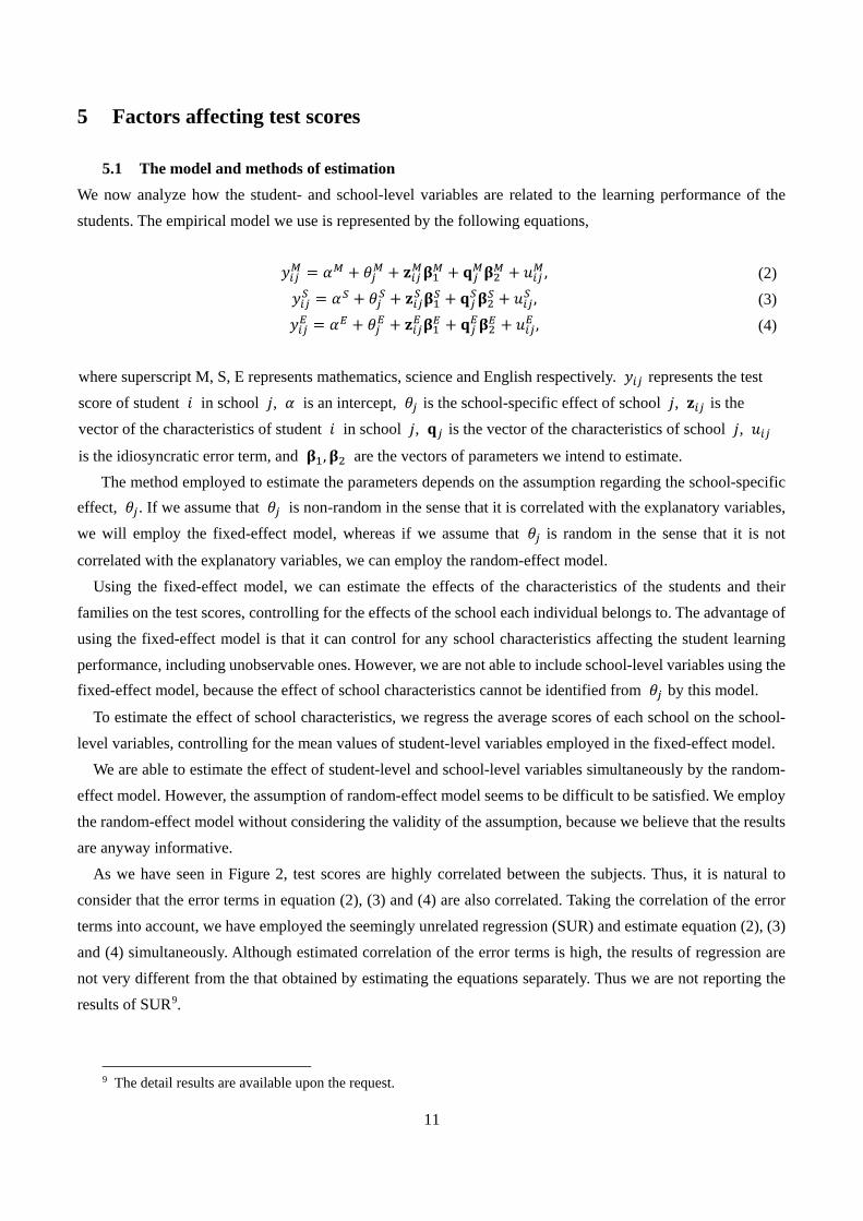
5 Factors affecting test scores 5.1 The model and methods of estimation

We now analyze how the student- and school-level variables are related to the learning performance of the students. The empirical model we use is represented by the following equations,

𝑡𝑡𝑖𝑖𝑖𝑖𝑀𝑀 = 𝛼𝛼𝑀𝑀 + 𝜃𝜃𝑖𝑖𝑀𝑀 + 𝐳𝐳𝑖𝑖𝑖𝑖𝑀𝑀𝛃𝛃1𝑀𝑀 + 𝐪𝐪𝑖𝑖𝑀𝑀𝛃𝛃2𝑀𝑀 + 𝑢𝑢𝑖𝑖𝑖𝑖𝑀𝑀, (2) 𝑡𝑡𝑖𝑖𝑖𝑖𝑆𝑆 = 𝛼𝛼𝑆𝑆 + 𝜃𝜃𝑖𝑖𝑆𝑆 + 𝐳𝐳𝑖𝑖𝑖𝑖𝑆𝑆 𝛃𝛃1𝑆𝑆 + 𝐪𝐪𝑖𝑖𝑆𝑆𝛃𝛃2𝑆𝑆 + 𝑢𝑢𝑖𝑖𝑖𝑖𝑆𝑆 , (3) 𝑡𝑡𝑖𝑖𝑖𝑖𝐸𝐸 = 𝛼𝛼𝐸𝐸 + 𝜃𝜃𝑖𝑖𝐸𝐸 + 𝐳𝐳𝑖𝑖𝑖𝑖𝐸𝐸 𝛃𝛃1𝐸𝐸 + 𝐪𝐪𝑖𝑖𝐸𝐸𝛃𝛃2𝐸𝐸 + 𝑢𝑢𝑖𝑖𝑖𝑖𝐸𝐸 , (4)

where superscript M, S, E represents mathematics, science and English respectively. 𝑡𝑡𝑖𝑖𝑖𝑖 represents the test score of student 𝑖𝑖 in school 𝑗𝑗, 𝛼𝛼 is an intercept, 𝜃𝜃𝑖𝑖 is the school-specific effect of school 𝑗𝑗, 𝐳𝐳𝑖𝑖𝑖𝑖 is the vector of the characteristics of student 𝑖𝑖 in school 𝑗𝑗, 𝐪𝐪𝑖𝑖 is the vector of the characteristics of school 𝑗𝑗, 𝑢𝑢𝑖𝑖𝑖𝑖

is the idiosyncratic error term, and 𝛃𝛃1,𝛃𝛃2 are the vectors of parameters we intend to estimate. The method employed to estimate the parameters depends on the assumption regarding the school-specific

effect, 𝜃𝜃𝑖𝑖. If we assume that 𝜃𝜃𝑖𝑖 is non-random in the sense that it is correlated with the explanatory variables, we will employ the fixed-effect model, whereas if we assume that 𝜃𝜃𝑖𝑖 is random in the sense that it is not

correlated with the explanatory variables, we can employ the random-effect model. Using the fixed-effect model, we can estimate the effects of the characteristics of the students and their

families on the test scores, controlling for the effects of the school each individual belongs to. The advantage of using the fixed-effect model is that it can control for any school characteristics affecting the student learning performance, including unobservable ones. However, we are not able to include school-level variables using the fixed-effect model, because the effect of school characteristics cannot be identified from 𝜃𝜃𝑖𝑖 by this model.

To estimate the effect of school characteristics, we regress the average scores of each school on the school-level variables, controlling for the mean values of student-level variables employed in the fixed-effect model.

We are able to estimate the effect of student-level and school-level variables simultaneously by the random-effect model. However, the assumption of random-effect model seems to be difficult to be satisfied. We employ the random-effect model without considering the validity of the assumption, because we believe that the results are anyway informative.

As we have seen in Figure 2, test scores are highly correlated between the subjects. Thus, it is natural to consider that the error terms in equation (2), (3) and (4) are also correlated. Taking the correlation of the error terms into account, we have employed the seemingly unrelated regression (SUR) and estimate equation (2), (3) and (4) simultaneously. Although estimated correlation of the error terms is high, the results of regression are not very different from the that obtained by estimating the equations separately. Thus we are not reporting the results of SUR9.

9 The detail results are available upon the request.

12

5.2 Fixed-effect model We now estimate the fixed-effect model. As discussed in the previous subsection, this model estimates the association of student-level variables with intra-school variation in learning performance. The variables we use to represent the characteristics of the student are gender, number of siblings, distance from home to school, whether the student has an undisturbed learning environment at home, whether the student uses English for communication at home, number of days absent from school, educational attainment of the parents, family income, number of books available for the student’s reading at home, and amount of private tuition fees spent on the student.

In addition, information about the student’s amount of time spent learning at home—on homework, receiving additional private instruction, self-study, etc.—is available for analysis. It should be noted, however, that using such information reduces the sample size by more than 30 percent due to the low response rate on these questions. Thus we estimate the model without information on the student’s time learning at home (model 1), and with it (model 2).

Table 6 shows the results for the fixed-effect estimation. In Sri Lanka, girls outperform boys on all three subjects, and the differences are statistically significant when we do not control for the student’s time spent learning at home. However once time spent learning at home is controlled for, the differences are not significant. This suggests that the girls study at home more than the boys do, and this is what explains differences in academic performance by gender.


Number of siblings correlates negatively with academic performance for all three subjects. We estimated the

coefficients of the number of elder siblings and the number of younger siblings separately, and found that the coefficients of the younger siblings are larger than those of the elder siblings. The coefficients are even larger in model 2, which controls for the student’s time used for learning at home, than in model 1, suggesting that students who have many siblings perform worse for some other reason than because they do not have enough time to study at home.

Distance from home to school does not correlate with scores in mathematics and science, but it does correlate with scores in English. The negative coefficients of home distance in English may suggest that students living in remote areas do not have many opportunities to use English and do not perform well in English.

Students who have an undisturbed learning environment at home perform significantly better. The effect is relatively large. Thus, it seems important to provide students with an undisturbed learning environment at home in order to improve their academic performance.

Students who speak English at home perform better not only in English but also in mathematics and science. This may reflect the generally high socioeconomic status of families using English, beyond what is already captured by family income, parental education, and so on.

13

The number of days absent from school does not decrease scores, and even increases them in some models. We cannot give a reasonable explanation for this.

The coefficients of family income are mostly statistically insignificant. This is because family income is closely correlated to parents’ education; if we exclude the parents’ education, the coefficients of family income variables became significant. Nevertheless, students from families with very high incomes perform well even after controlling for parents’ education.

The coefficients of parents’ educational attainment are mostly significant, even after controlling for income. Students whose parents have higher educational background are more likely to perform well.

The number of books available to the student at home and the amount of private tuition fees spent on the student both have significant coefficients, as expected. These variables can be viewed as measuring the socioeconomic status of the family and how much the parents care about their children’s education. The results suggest that the amount of resource spent on education by parents plays an important role in children’s academic performance.

The time spent on homework also significantly affects students’ academic performance. Students who spend 15 to 30 minutes on homework daily perform better than who spend no time on homework, and students who spend 30 minutes to 1 hour perform even better. However, students who spend more than 1 hour on homework perform only as well as those who spend 15–30 minutes. This suggests that efficient time use on homework is important for the better academic performance. The coefficients are relatively large in science and mathematics, but small in English.

The time spent on private tuition has a significant effect only if it is more than 1 hour. Combined with the insignificant coefficient for days of absence from school and the significant coefficient of tuition fees, this result suggests that private tuition works as a supplement to public school and plays an important role in the academic performance of the students. It should be also noted that time spent on self-learning has a significant effect only in science.

5.3 School-level variables and test scores In this section, we estimate the effects of school characteristics on the academic performance of students. To do so, we first regress the mean scores by school on the mean values of the explanatory variables employed in the fixed-effect model; then, we add the school-level variables to the set of explanatory variables. Finally, we apply the mixed-effect model.

Table 7 shows the results of the regressions on the school mean. In model 1, we use as a set of explanatory variables the means of the variables used in the fixed-effect model, with some variables that turned out to be insignificant in the fixed-effect model omitted. The results are mostly the same as in the fixed-effect model, suggesting that the factors explaining the within-school variation of test scores also explain between-school variation. The important difference is that the coefficients of mean log value for days of absence become negative (and significant in mathematics), suggesting that students in schools where many students are frequently absent perform not so well, although absence does not affect the individual absent student’s test score.

14


In model 2, we include school-level variables: index of school facilities, number of students in the classroom,

number of students in grade 8 in the school, proportion of students who have ever had their property stolen in the classroom, and proportion of students who had ever experienced violence in the classroom. Including school characteristics does not change the coefficients of the student-level variables much, although some coefficients are attenuated; the signs of the coefficients of the school-level variables are mostly as expected, and they are statistically significant. However, the index of school facilities is significant only in science, plausibly because studying science requires more facilities than studying mathematics or English. Finally, the coefficients of number of students in the classroom and number of students in grade 8 are somehow mixed. Because class size and the school size could be endogenous, we cannot interpret these coefficients simply. Regardless, overall, stealing and violence in the classroom correlate negatively with academic performance, as expected.

In model 3, we add the characteristics of the teachers of each subject and the principal of the school. Most coefficients are not significant. This may suggest that the characteristics of teachers and principal are not associated with student learning performance. s. The insignificance of the coefficients here could possibly have several causes. First, these students are in grade 8 and would have been taught by many teachers in their school careers so far. Thus, the characteristics of their current teachers will carry less weight for their current academic performance. Second, teachers and principals are not randomly assigned. For example, students who do not perform well may possibly be assigned to good teachers, and principals who have got a good reputation may be sent to schools with low learning performance. Such endogeneity might affect the results. To identify the effect of the teacher precisely, we need information about all teachers who have taught the student. Although we have information on average characteristics of the teachers in the school (education attainment, qualification, attendance, attitude, and so on) from the principal questionnaire, the response rate was low and the measurement errors are problematically large. Thus, we omitted these from the analysis.

Table 8 shows the results of mixed-effect regressions. We estimated three models for each subject, with the underlying assumption is that school-specific effects are not correlated with the explanatory variables. The results are mostly consistent with those of the fixed-effect model and regression on school means (Table 6 and Table 7). However, the teacher and school characteristics are not significantly correlated with the test scores. We discuss the results further in the conclusion.


6 Conclusion

In this paper, we examined students’ family background, school choice, and academic performance. The findings can be summarized as follows. First, there is a large difference in test scores between Type 1AB schools

15

and other types of schools. Students from families with high socioeconomic status are more likely to be in Type 1AB schools, and the treatment effects of attending Type 1AB school on academic performance are large. These results suggest that for students of low socioeconomic status, the opportunity to achieve better academic performance is limited. Second, the fixed-model results suggest that the socioeconomic status of the student’s family is also closely correlated to students’ test scores. In contrast, there is no clear evidence that teacher and school characteristics other than type of school are associated with academic performance.

It is worth discussing why teacher and school characteristics are not associated with academic performance. If differences in academic performance between Type 1AB and the other schools are due to differences in the quality in education provided, the characteristics of the schools should also differ in consistent and significant ways. However, no clear effects of teacher and school characteristics on students’ academic performance were observable in the data, especially given the issue of measurement error mentioned above. If teachers are allocated in light of characteristics that are unobservable in the present research, it may be these qualities that correlate with the academic performance of the students, remaining uncaptured by the data.

It is also important to be aware of the limitations of our dataset. Although the present survey is well designed to assess academic performance, the measurement error is quite large. Many responses are inconsistent with one another, which may attenuate the regression coefficients. Aturupane et al. (2013) pointed out the problem of measurement error in the NEREC test score data from 2002. They argued that the teacher and school variables in particular contain inconsistent and missing values because teachers and principals completed the questionnaire without any assistance. Aturupane et al. (2013) addressed this problem using an additional dataset collected by National Education Commission (NEC), providing more detailed information for a random subsample of the NEREC respondents. Since the NEC survey was conducted by trained interviewers, the collected information should be more accurate. Aturupane et al. (2013) used teacher and school variables from the NEC, but most of them did not turn out to be significant. Therefore, the differences between Type 1AB schools and other types of schools remain mostly unobservable and are not captured by the survey.

In addition, since the data were obtained by the survey at specific point in time and are therefore not experimentally sound, the coefficients estimated in the regression models might not be interpreted as causal effects on the test scores. However, our results at least tell us what kind of students we need to pay more attention to in strengthening education system, that is, what kind of students are left behind. Our results suggest that students from families with low socioeconomic status, who do not have enough educational resources at home are the ones who tend to be left behind and to need special attention and care in their education. However, we still need to further investigate the relevance of differences in teacher and school characteristics for difference in academic performance between Type 1AB and other types of schools. This will be done in future research.

16

References

Aturupane, H., P. Glewwe, and S. Wisniewski. 2013. “The Impact of School Quality, Socioeconomic Factors, and Child Health on Students’ Academic Performance: Evidence from Sri Lankan Primary Schools.” Education Economics 21 (1): 2-37.

Coleman, J.S., E.Q. Campbell, C.J. Hobson, J. McPartland, A.M. Mood, and F.D. Weinfield. 1966. Equality of Educational Opportunity. Washington, DC: National Centre for Educational Statistics.

Glewwe, P.W., E.A. Hanushek, S.D. Humpage, and R. Ravina. 2011. “School Resources and Educational Outcomes in Developing Countries: A Review of the Literature from 1990 to 2010.” NEBR Working Paper 17554. Cambridge, MA: National Bureau of Economic Research.

Hanushek, E.A. 1995. “Interpreting Recent Research on Schooling in Developing Countries.” World Bank Research Observer 10: 227-246.

Hanushek, Eric A., and Dennis D. Kimko. 2000. “Schooling, Labor-Force Quality, and the Growth of Nations.” American Economic Review 90 (5): 1184–1208.

Hanushek, Eric A., and Ludger Wößmann. 2007. “The Role of Education Quality for Economic Growth.” World Bank Policy Research Working Paper, no. 4122.

Hanushek, Eric A., and Ludger Wößmann, 2012. ‘’Schooling, educational achievement, and the Latin American growth puzzle.’’ Journal of Development Economics, 99(2): 497–512.

Heyneman, S.P. and W.A. Loxley. 1983. “The Effect of Primary-School Quality on Academic Achievement across 29 High-Income and Low-Income Countries.” American Journal of Sociology 88 (6): 1162–1194.

Himaz, R. 2010. “Intra-Household Allocation of Education Expenditure: The Case of Sri Lanka.” Economic Development and Cultural Change 58: 231-258.

Imbens, G. W. 2015. “Matching methods in practice: Three examples.” Journal of Human Resources, 50 (2): 373–419.

Little, A., H., Aturupane, and M. Shojo. 2013. “Transforming Primary Education in Sri Lanka: From a ‘Subject’ of Education to a ‘Stage’ of Education.” South Asia Human Development Unit Discussion Paper Series 61. Washington, DC: World Bank.

National Education Research and Evaluation Centre (NEREC). 2013. National Assessment of Achievement of Grade 8 Students in Sri Lanka—2012. Colombo: NEREC.

Rothstein, R. 2000. Finance Fungibility: Investing Relative Impacts of Investments in Schools and Non-School Educational Institutions to Improve Student Achievement. Washington, DC: Centre on Educational Policy Publications.

17

United Nations Educational, Scientific, and Cultural Organization (UNESCO). 2014. EFA Monitoring Report 2013/14. Teaching and Learning: Achieving Quality for All. Paris: UNESCO.

World Bank. 2011a. Transforming School Education in Sri Lanka: From Cut Stones to Polished Jewels. Washington, DC: World Bank.

World Bank. 2011b. World Bank Group Education Strategy 2020. Washington, DC: World Bank.

World Bank. 2015. Transforming the School Education System as the Foundation of a Knowledge Hub: P113488 - Implementation Status Results Report; Sequence 08. Washington, DC: World Bank.

Table 1. Distributions of test scores

Table 2. Descriptive statistics

Obs Mean Std Dev Min 10% 25% 50% 75% 90% MaxMathematics 12,814 51.4 21.0 0.0 25.0 35.0 47.5 67.5 82.5 97.5Science 12,874 41.9 21.4 0.0 16.0 25.0 39.0 58.0 81.0 100.0English 12,817 40.0 23.3 0.0 16.0 22.0 32.0 56.0 80.0 100.0

Location Municipal 0.132Urban 0.094Pradeshiya Sabha 0.774

School type Type 1AB 0.363(base=1AB) Type 1C 0.397

Type 2 0.240

School managemet National 0.218Provincial 0.782

Language Sinhala 0.671Tamil 0.329

School facilities 15.039(9.243)

Number of students in the classroom 33.998(8.669)

Number of students in grade 8 112.599(93.075)

Stealing in the classroom 0.382(0.191)

Violence in the classroom 0.372(0.162)

(b) school-level variables

Gender Male 0.483Female 0.517

Number of elder siblings 0.910(1.165)

Number of younger siblings 1.272(1.596)

Distance from school Less than 15 min 0.30915 ― 30 min 0.35030 min ―1 hour 0.233More than 1 hour 0.108

Home environment 0.081Using English 0.617Days of absence 16.977

(20.122)

Time spent on homework Less than 15min 0.13515 ― 30 min 0.32630 min ― 1 hour 0.341More than 1 hour 0.198

Time spent for tuition Less than 15min 0.09715 ― 30 min 0.14130 min ― 1 hour 0.239More than 1 hour 0.523

Time spent for self- Less than 15min 0.221 learning 15 ― 30 min 0.354

30 min ― 1 hour 0.255More than 1 hour 0.170

Family income < Rs.10,000 0.405Rs.10,001― Rs.20,000 0.298Rs.20,001― Rs.30,000 0.149Rs.30,001― Rs.40,000 0.066Rs.40,001― Rs.50,000 0.039Rs.50,001― 0.043

Mother's education No education 0.062Up to Grade 5 0.182Up to Grade 10 0.203GCE O/L 0.302GCE A/L 0.133Vocational course post O/L or A/L 0.080Bachelor's Degree 0.019Post-graduation and above 0.019

Father's education No education 0.058Up to Grade 5 0.158Up to Grade 10 0.179GCE O/L 0.335GCE A/L 0.146Vocational course post O/L or A/L 0.085Bachelor's Degree 0.020Post-graduation and above 0.018

Tuition fees 4,438(8858)

Number of books for mathematics at home 1.924(14.589)

Number of books for science at home 2.492(18.991)

Number of books for English at home 2.863(1.165)

(a) student―level variables

Mathematics teacherGender Male 0.425

Female (0.575)

Years of teaching 14.117(10.653)

Education GCE O/L 0.083GCE A/L 0.614Bachelor's Degree 0.235Master's Degree 0.068

Time spent for lesson planning 1.767(hours) (1.453) Remedial teaching 0.752

Science teacherGender Male 0.275

Female 0.725


Education GCE O/L 0.044GCE A/L 0.642Bachelor's Degree 0.227Master's Degree or higher 0.086


English teacherGender Male 0.254

Female 0.746


Education GCE O/L 0.075GCE A/L 0.714Bachelor's Degree 0.163Master's Degree 0.049


PrincipalGender Male 0.855

Female 0.145

Years of experience as a principal 10.885(7.331)

Education GCE O/L 0.044GCE A/L 0.274Bachelor's Degree 0.333Master's Degree 0.331Ph.D. 0.017

(c) teacher and principal

Table 3. Results of OLS Regression

(a) Mathematics

Note: Standard errors in parenthesis. ***, **, * indicate that the coefficients are statistically significant at 1%, 5%, 10% level. Standard errors are clustered at school-level. Sampling weights are used to obtain the coefficients and standard errors.

(1) (2) (3) (4) (5) (6)

Province Central -3.563 -2.030(base=Western) (3.406) (2.301)

Eastern -6.283 -1.067(3.830) (2.815)

Northern -3.973 0.238(3.686) (2.837)

North Western -1.963 0.353(3.742) (2.415)

Northern Central -7.605 ** -1.895(3.313) (2.279)

Sabaragamuwa -2.147 -0.227(3.555) (2.143)

Southern -0.026 -0.754(3.383) (2.155)

Uva -8.477 ** -5.852 **(3.765) (2.531)

Location Urban -2.708 0.790(base=Municipal) (3.102) (2.156)

Pradeshiya Sabha -16.924 *** -8.608 ***(2.227) (1.748)

School type 1C -19.402 *** -8.405 ***(base=1AB) (1.320) (1.728)

Type 2 -22.786 *** -11.928 ***(1.426) (1.851)

School managemet National 20.991 *** 12.619 ***(base=Provincial) (1.462) (1.793)Language Tamil -4.611 ** -0.102(base=Sinhala) (1.946) (1.278)

Constant 54.765 *** 63.398 *** 61.121 *** 44.200 *** 52.637 *** 58.583 ***(2.302) (2.041) (1.153) (0.737) (1.061) (2.323)

Observations 12,814 12,814 12,814 12,814 12,814 12,814R-squared 0.020 0.125 0.242 0.226 0.009 0.328

(b) Science

Note: Standard errors in parenthesis. ***, **, * indicate that the coefficients are statistically significant at 1%, 5%, 10% level. Standard errors are clustered at school-level. Sampling weights are used to obtain the coefficients and standard errors.

(1) (2) (3) (4) (5) (6)

Province Central -2.623 -0.711(base=Western) (3.390) (2.490)

Eastern -5.862 1.276(3.904) (2.906)

Northern -6.193 * 0.257(3.155) (2.760)

North Western -1.650 0.493(3.570) (2.461)

Northern Central -3.264 1.961(3.502) (2.264)

Sabaragamuwa -1.222 0.985(3.480) (2.335)

Southern 3.386 2.242(3.329) (2.313)

Uva -6.659 * -3.972(3.609) (2.610)

Location Urban -5.531 * -1.460(base=Municipal) (3.246) (2.166)



Type 2 -22.052 *** -10.891 ***(1.514) (1.837)

School managemet National 20.450 *** 12.199 ***(base=Provincial) (1.547) (1.827)Language Tamil -7.594 *** -2.918 **(base=Sinhala) (1.865) (1.344)

Constant 44.015 *** 53.953 *** 51.151 *** 34.865 *** 43.908 *** 48.376 ***(2.199) (2.187) (1.203) (0.655) (1.050) (2.456)


(c) English

Note: Standard errors in parentheses. ***, **, * indicate that the coefficients are statistically significant at 1%, 5%, 10% level. Standard errors are clustered at school level. Sampling weights are used to obtain the coefficients and standard errors.

(1) (2) (3) (4) (5) (6)

Province Central -0.835 0.792(base=Western) (4.651) (3.176)

Eastern -13.601 *** -9.629 ***(3.976) (3.237)

Northern -9.173 ** -7.003 *(4.477) (3.628)

North Western -3.880 0.137(4.478) (2.693)

Northern Central -12.700 *** -4.593(4.008) (2.907)

Sabaragamuwa -2.807 0.327(5.016) (2.971)

Southern -2.771 -2.356(4.167) (2.539)

Uva -6.845 -2.689(5.164) (3.322)

Location Urban -2.419 1.324(base=Municipal) (4.375) (3.227)



Type 2 -26.268 *** -13.355 ***(1.720) (2.029)

School managemet National 24.426 *** 12.991 ***(base=Provincial) (2.124) (2.342)Language Tamil -5.835 ** 3.100(base=Sinhala) (2.532) (2.543)

Constant 45.253 *** 56.378 *** 51.678 *** 31.625 *** 41.558 *** 52.160 ***(2.953) (2.583) (1.610) (0.944) (1.346) (3.001)


Table 4. Probit model of school choice

Table 5. Results of propensity score matching

Dependent variable: School type(1: Type 1AB, 0: Type 1C and Type 2)

Log (number of books) 0.074 ***Gender Male 0.095 (0.015)(base=female) (0.069) Log (tuition fees) 0.047 ***Mother's education No education -0.270 ** (0.007)(base=GCE O/L) (0.113) Num. of siblings -0.071 ***

Up to Grade 5 -0.435 *** (0.015)(0.059) Province Central 0.189

Up to Grade 10 -0.264 *** (base=Western) (0.291)(0.049) Eastern 0.266

GCE A/L 0.274 *** (0.335)(0.047) Northern 0.493 *

Vocational course 0.224 *** (0.288) post O/L or A/L (0.071) North Western 0.222Bachelor's Degree 0.196 * (0.289)

(0.115) Northern Central 0.238Post-graduation 0.255 * (0.301) and above (0.133) Sabaragamuwa 0.140Unkown -0.210 ***

(0.069)Father's education No education -0.333 *** (0.296)(base=GCE O/L) (0.097) Southern 0.435

Up to Grade 5 -0.359 *** (0.288)(0.077) Uva 0.443

Up to Grade 10 -0.212 *** (0.291)(0.052) Location Urban -0.421

GCE A/L 0.271 *** (base=Municipal) (0.294)(0.055) Pradeshiya Sabha -0.951 ***

Vocational course 0.252 *** (0.213) post O/L or A/L (0.071) Constant 0.137 *Bachelor's Degree 0.473 *** (0.264)

(0.132)Post-graduation 0.487 *** Observations 11,101 and above (0.147)Unkown -0.162 **

(0.076)Family income Rs.10,001― 0.130 ***(base = < Rs.10,000) Rs.20,000 (0.048)

Rs.20,001― 0.320 *** Rs.30,000 (0.059)Rs.30,001― 0.363 *** Rs.40,000 (0.079)Rs.40,001― 0.547 *** Rs.50,000 (0.100)Rs.50,001― 0.425 ***

(0.106)

Number ofobservations

Average treatment effect(standard error)

Mathematics 10,956 8.084(0.468)

Science 10,702 6.654(0.498)

English 10,968 10.022(0.595)

Table 6. Fixed-effect model

Gender Male -1.190 *** -0.809 -1.915 *** -1.104 * -3.641 *** -3.560 ***(base=female) (0.404) (0.516) (0.436) (0.563) (0.418) (0.522)Number of elder siblings -0.348 ** -0.248 -0.819 *** -0.787 *** -0.458 *** -0.468 **

(0.153) (0.203) (0.167) (0.243) (0.145) (0.195)Number of younger siblings -0.628 *** -0.670 *** -0.816 *** -0.790 *** -0.517 *** -0.664 ***

(0.093) (0.122) (0.108) (0.131) (0.096) (0.141)Distance from school 15 ― 30 min -0.173 -0.316 0.390 0.132 -0.584 -0.873 *(base=less than 15 min) (0.400) (0.512) (0.420) (0.547) (0.381) (0.495)

30 min ― 1 hour 0.252 -0.127 1.227 ** 0.805 -1.023 ** -1.831 ***(0.494) (0.612) (0.531) (0.650) (0.503) (0.635)

More than 1 hour -0.646 -0.771 -0.739 -1.029 -1.537 ** -2.364 **(0.618) (0.812) (0.722) (0.871) (0.683) (0.935)

Home environment -3.942 *** -3.871 *** -5.021 *** -3.877 *** -2.797 *** -2.079 ***(0.605) (0.948) (0.617) (0.993) (0.500) (0.771)

Using English 1.074 *** 1.213 ** 0.990 ** 1.025 * 2.789 *** 3.090 ***(0.392) (0.517) (0.411) (0.570) (0.409) (0.549)

Log(days of absense) 0.345 * -0.226 0.435 ** 0.300 0.497 *** 0.356 *(0.183) (0.214) (0.199) (0.279) (0.163) (0.209)

Time spent on homework 15 ― 30 min 3.332 *** 3.848 *** 2.317 ***(base=less than 15 min) (0.711) (0.769) (0.592)

30 min ― 1 hour 4.233 *** 5.111 *** 2.634 ***(0.707) (0.788) (0.659)

More than 1 hour 2.881 *** 3.958 *** 0.546(0.779) (0.780) (0.796)

Time spent for tuition 15 ― 30 min 0.228 1.148 0.964(base=less than 15 min) (0.829) (0.980) (0.727)

30 min ― 1 hour 1.558 * 0.914 0.856(0.793) (0.814) (0.683)

More than 1 hour 4.143 *** 3.336 *** 3.572 ***(0.801) (0.803) (0.722)

Time spent for self- 15 ― 30 min 0.092 1.446 ** 0.530 learning (0.529) (0.615) (0.486)(base=less than 15 min) 30 min ― 1 hour -0.289 1.840 *** 0.225

(0.634) (0.679) (0.585)More than 1 hour -0.147 1.162 -0.688

(0.665) (0.801) (0.690)Family income Rs.10,001― 0.476 -0.195 0.266 -0.180 0.252 -0.079(base = < Rs.10,000) Rs.20,000 (0.363) (0.491) (0.399) (0.562) (0.368) (0.559)

Rs.20,001― 0.651 -0.200 1.052 * 0.715 0.946 * 0.388 Rs.30,000 (0.498) (0.615) (0.541) (0.707) (0.556) (0.695)Rs.30,001― 0.649 -0.286 0.808 0.808 1.231 * 0.523 Rs.40,000 (0.730) (0.845) (0.810) (0.970) (0.700) (0.818)Rs.40,001― 0.414 -0.459 2.628 ** 2.105 * 2.420 ** 1.542 Rs.50,000 (0.832) (0.947) (1.143) (1.192) (0.976) (1.071)Rs.50,001― 1.189 0.295 2.335 ** 2.048 3.962 *** 4.240 ***

(0.888) (1.098) (1.146) (1.334) (1.005) (1.131)

Mathematics Science Englishmodel 1 model 2 model 1 model 2 model 1 model 2

Note: Standard errors in parentheses. ***, **, * indicate that the coefficients are statistically significant at 1%, 5%, 10% level. Standard errors are clustered at school level. Sampling weights are used to obtain the coefficients and standard errors.

Mother's education No education -2.656 *** -1.879 -1.579 ** -1.783 * -1.700 *** -1.319(base=GCE O/L) (0.741) (1.146) (0.742) (0.998) (0.581) (0.902)

Up to Grade 5 -2.700 *** -2.722 *** -2.395 *** -2.043 *** -1.854 *** -1.804 ***(0.558) (0.720) (0.581) (0.776) (0.440) (0.604)

Up to Grade 10 -2.187 *** -2.741 *** -2.111 *** -2.024 *** -1.720 *** -1.724 ***(0.503) (0.622) (0.545) (0.767) (0.425) (0.573)

GCE A/L 1.301 ** 1.417 ** 1.868 *** 1.247 * 1.447 ** 1.252 *(0.520) (0.605) (0.596) (0.737) (0.599) (0.729)

Vocational course 0.988 0.762 1.802 ** 1.878 ** 1.215 1.092 post O/L or A/L (0.710) (0.776) (0.806) (0.942) (0.785) (0.816)Bachelor's Degree 2.576 ** 1.711 4.664 *** 3.745 * 3.686 ** 2.101

(1.224) (1.385) (1.681) (2.117) (1.558) (1.750)Post-graduation 4.728 *** 4.149 *** 5.328 *** 4.544 ** 5.709 *** 5.113 *** and above (1.387) (1.378) (1.606) (1.816) (1.414) (1.476)Unkown -1.584 *** -2.010 ** -1.895 *** -1.863 ** -1.222 ** -0.793

(0.592) (0.798) (0.600) (0.854) (0.496) (0.752)Father's education No education -1.585 * -1.647 -3.553 *** -2.593 ** -1.517 ** -0.931(base=GCE O/L) (0.821) (1.318) (0.791) (1.143) (0.641) (0.991)

Up to Grade 5 -1.794 *** -1.544 ** -2.980 *** -2.169 *** -0.686 -0.343(0.527) (0.744) (0.549) (0.815) (0.452) (0.580)

Up to Grade 10 -1.242 *** -1.077 * -2.178 *** -1.670 ** -0.556 -0.519(0.469) (0.647) (0.473) (0.728) (0.468) (0.651)

GCE A/L 2.680 *** 2.397 *** 3.621 *** 4.375 *** 2.493 *** 2.395 ***(0.514) (0.602) (0.540) (0.717) (0.612) (0.732)

Vocational course 2.466 *** 2.541 *** 1.783 ** 1.821 * 2.314 *** 1.921 ** post O/L or A/L (0.694) (0.791) (0.779) (0.982) (0.672) (0.813)Bachelor's Degree 6.363 *** 6.638 *** 5.345 *** 7.219 *** 5.598 *** 4.521 ***

(1.197) (1.200) (1.520) (1.802) (1.383) (1.564)Post-graduation 5.800 *** 5.910 *** 6.368 *** 6.657 *** 3.317 ** 3.460 ** and above (1.250) (1.374) (1.615) (1.734) (1.330) (1.557)Unkown -2.124 *** -1.425 -2.917 *** -1.702 * -0.096 0.727

(0.693) (0.981) (0.760) (1.028) (0.729) (1.171)Log (tuition fees) 4.811 *** 4.189 *** 4.276 *** 4.922 *** 2.314 *** 2.507 ***

(0.394) (0.563) (0.389) (0.598) (0.380) (0.546)Log (number of books at home) 0.497 *** 0.512 ** 0.586 *** 0.739 *** -0.568 *** -0.554 ** any book (0.173) (0.208) (0.203) (0.264) (0.193) (0.243)Log (number of books at home) 0.670 ** 0.476 1.135 *** 0.672 2.765 *** 2.772 *** books for the subject (0.316) (0.363) (0.345) (0.430) (0.327) (0.392)Constant 47.634 *** 46.365 *** 38.359 *** 32.512 *** 37.461 *** 36.429 ***

(0.778) (1.307) (0.840) (1.472) (0.760) (1.250)

R 2 within 0.091 0.096 0.115 0.126 0.110 0.117between 0.683 0.607 0.666 0.654 0.728 0.606overall 0.320 0.304 0.333 0.335 0.366 0.333

σ u 10.647 10.763 9.716 10.176 13.462 13.644σ e 13.908 14.086 14.647 15.078 13.132 13.750ρ 0.369 0.369 0.306 0.313 0.512 0.496

Observations 10,527 7,062 10,294 6,351 10,542 6,655Number of school 436 432 436 431 436 432

Table 7. Regression on school mean

Gender Male 1.763 2.901 * 4.440 ** -0.894 0.851 1.485 -3.033 ** -2.362 -1.341(base=female) (1.403) (1.479) (1.729) (1.520) (1.572) (1.874) (1.469) (1.564) (1.855)Number of elder siblings -1.604 -1.369 -1.347 -1.699 -1.197 -1.358 -2.638 ** -2.575 ** -2.568 **

(0.983) (0.984) (0.990) (1.084) (1.066) (1.124) (1.022) (1.035) (1.087)Number of younger siblings -2.042 *** -1.970 *** -2.010 *** -2.447 *** -2.170 *** -1.790 ** -1.580 ** -1.560 ** -1.158

(0.644) (0.640) (0.648) (0.699) (0.682) (0.725) (0.678) (0.681) (0.706)Distance from school 15 ― 30 min -7.604 *** -8.089 *** -8.820 *** -8.032 *** -7.116 *** -6.831 ** -9.379 *** -9.974 *** -8.092 ***(base=less than 15 min) (2.548) (2.554) (2.646) (2.785) (2.738) (2.877) (2.647) (2.685) (2.862)

30 min ― 1 hour 0.486 -0.741 -5.018 * 4.455 2.674 0.524 1.624 1.111 -1.053(2.702) (2.689) (2.769) (2.954) (2.882) (3.143) (2.792) (2.811) (3.034)

More than 1 hour -6.068 -9.020 ** -11.370 *** -4.348 -6.988 * -7.841 * -4.076 -5.808 -5.632(3.841) (3.880) (4.144) (4.149) (4.100) (4.546) (3.988) (4.083) (4.415)

Home environment -8.081 *** -9.712 *** -9.344 *** -11.072 *** -12.410 *** -12.016 *** -6.304 ** -7.376 ** -6.921 **(3.046) (3.044) (3.056) (3.358) (3.290) (3.448) (3.173) (3.209) (3.342)

Using English 1.283 1.614 -0.049 -0.151 0.517 -0.753 3.876 ** 4.049 ** 2.812(1.778) (1.770) (1.850) (1.924) (1.879) (2.017) (1.855) (1.868) (2.012)

Log (days of absense) -1.646 *** -1.584 *** -1.731 *** -0.466 -0.344 -0.692 -0.165 -0.154 -0.138(0.570) (0.568) (0.589) (0.619) (0.604) (0.661) (0.590) (0.595) (0.632)

Mother's Education Up to Grade 5 -1.597 -1.566 1.214 -2.511 -4.001 -3.274 -4.438 -3.960 -0.451(base=no education) (6.608) (6.559) (6.630) (7.286) (7.088) (7.710) (6.839) (6.869) (7.154)

Up to Grade 10 -3.175 -2.141 -2.450 2.863 2.184 2.677 -4.190 -3.118 -1.251(6.422) (6.372) (6.461) (6.990) (6.795) (7.416) (6.656) (6.686) (6.924)

GCE O/L 3.799 2.997 7.503 7.362 5.516 9.578 -6.073 -5.967 -2.326(6.561) (6.494) (6.532) (7.151) (6.945) (7.500) (6.790) (6.802) (7.056)

GCE A/L 15.005 ** 12.629 * 11.937 14.075 * 11.633 12.230 20.113 *** 18.901 ** 23.199 ***(7.344) (7.305) (7.522) (8.037) (7.855) (8.454) (7.637) (7.677) (8.166)

Vocational course 10.741 9.694 13.099 17.614 * 15.582 * 12.587 15.311 * 14.885 14.437 post O/L or A/L (8.752) (8.668) (9.144) (9.465) (9.205) (10.259) (9.100) (9.118) (9.782)Bachelor's Degree 6.504 4.584 27.912 * 13.408 10.992 51.172 *** -0.793 -0.333 11.996

(13.169) (13.080) (14.415) (13.100) (12.721) (16.299) (13.616) (13.691) (15.820)Post-graduation 22.623 * 21.563 18.828 21.291 20.381 35.556 ** 13.961 13.711 16.314 and above (13.398) (13.242) (13.484) (14.685) (14.236) (15.736) (13.887) (13.891) (14.615)

Father's Education Up to Grade 5 1.245 2.397 0.754 -5.315 -3.128 -4.590 2.675 3.126 0.191(base=no education) (6.259) (6.214) (6.295) (6.997) (6.811) (7.201) (6.534) (6.569) (6.831)

Up to Grade 10 5.361 5.647 5.617 -3.114 -1.018 -2.556 10.944 10.479 9.934(6.710) (6.640) (6.659) (7.372) (7.160) (7.815) (6.955) (6.970) (7.176)

GCE O/L 0.497 -0.394 -0.930 -0.333 -0.788 -3.123 1.960 1.136 -1.058(6.163) (6.098) (6.160) (6.748) (6.551) (7.103) (6.369) (6.380) (6.614)

GCE A/L 24.799 *** 23.372 *** 25.271 *** 8.065 7.545 5.378 29.693 *** 28.964 *** 26.409 ***(7.292) (7.232) (7.576) (7.999) (7.777) (8.495) (7.573) (7.599) (8.095)

Vocational course 13.713 12.216 3.769 -0.834 -1.317 -3.711 28.343 *** 27.711 *** 25.886 *** post O/L or A/L (8.679) (8.587) (9.008) (9.324) (9.050) (9.822) (9.072) (9.077) (9.617)Bachelor's Degree 50.453 *** 47.228 *** 42.178 *** 45.395 *** 47.301 *** 42.510 ** 55.346 *** 51.918 *** 47.346 ***

(13.467) (13.438) (15.070) (14.859) (14.545) (16.953) (13.939) (14.065) (16.075)Post-graduation 24.552 * 26.019 * 21.962 32.768 ** 33.403 ** 10.900 60.090 *** 60.796 *** 51.915 *** and above (14.359) (14.299) (14.816) (16.138) (15.750) (17.030) (14.844) (14.950) (16.111)

Log (tuition fees) 2.011 *** 1.871 *** 1.962 *** 1.645 *** 1.566 *** 1.604 *** 0.918 *** 0.862 *** 0.817 ***(0.236) (0.249) (0.255) (0.252) (0.262) (0.284) (0.247) (0.263) (0.286)

Log (number of books at home) -1.493 -1.918 * -1.459 -2.937 ** -3.793 *** -2.125 -5.892 *** -5.865 *** -5.691 *** any book (1.109) (1.109) (1.177) (1.338) (1.318) (1.440) (1.246) (1.258) (1.337)Log (number of books at home) 2.771 2.765 2.372 7.572 *** 7.824 *** 5.109 * 13.586 *** 13.158 *** 11.659 *** books for the subject (2.489) (2.472) (2.559) (2.593) (2.531) (2.701) (2.381) (2.405) (2.586)School facilities -0.010 0.023 0.069 * 0.075 -0.045 -0.066

(0.036) (0.043) (0.039) (0.049) (0.038) (0.047)Log(number of students in the class) 0.418 -0.265 4.100 ** 3.593 * -0.982 -0.069

(1.630) (1.685) (1.743) (1.894) (1.721) (1.842)Log(number of students in the grade) 1.758 ** 1.730 ** 0.712 0.555 1.154 1.116

(0.757) (0.820) (0.813) (0.894) (0.803) (0.878)Stealing in the classroom -3.854 * -2.767 -2.449 -0.469 -3.187 -2.408

(2.181) (2.260) (2.336) (2.568) (2.285) (2.470)Violence in the classroom -4.538 * -4.823 * -9.551 *** -8.735 *** -1.138 -1.427

(2.492) (2.621) (2.653) (2.822) (2.626) (2.748)

model 3Mathematics Science English

model 1 model 2 model 3 model 1 model 2 model 3 model 1 model 2

Note: Standard errors in parentheses. ***, **, * indicate that the coefficients are statistically significant at 1%, 5%, 10% level. Standard errors are clustered at school-level. Sampling weights are used to obtain the coefficients and standard errors.

Teacher variablesGender Male 0.284 -0.312 -0.730(base=female) (0.731) (0.865) (0.861)Years of teaching 0.026 -0.144 0.033

(0.123) (0.137) (0.157)Years of teaching squared -0.002 0.003 -0.001

(0.004) (0.004) (0.005)Education GCE A/L 0.170 0.079 -0.656(base=GCE O/L) (1.397) (1.955) (1.501)

Bachelor's Degree 0.735 -0.326 -1.353(1.551) (2.123) (1.820)

Master's Degree 0.155 -0.872 0.240(1.886) (2.332) (2.272)

Ph.D. -12.026(8.326)

Remedial Teaching 1.304 1.170 0.464(0.808) (0.875) (0.832)

Log (time spent for lesson planning) -0.136 0.083 0.048(0.241) (0.261) (0.260)

Principal variablesGender Male -0.065 1.158 -2.179 *(base=female) (1.081) (1.164) (1.179)Years of experience as a principal 0.261 0.114 -0.059

(0.173) (0.189) (0.186)Years of experience as a principal squared -0.008 -0.001 0.003

(0.007) (0.008) (0.008)Education GCE A/L -0.507 -2.512 -0.984(base=GCE O/L) (1.785) (1.961) (1.848)

Bachelor's Degree -0.599 -1.821 0.534(1.794) (1.995) (1.873)

Master's Degree -1.401 -1.189 0.567(1.805) (1.987) (1.880)

Ph.D. -0.813 0.149 5.725 *(3.236) (3.391) (3.463)

Constant 37.106 *** 33.217 *** 32.993 *** 32.798 *** 19.657 ** 20.874 ** 27.120 *** 28.677 *** 27.638 ***(5.750) (7.467) (7.854) (6.437) (8.190) (9.510) (6.063) (7.887) (8.608)

Observations 435 435 385 435 435 378 435 435 382R 2 0.778 0.787 0.796 0.726 0.746 0.761 0.834 0.836 0.830

Table 8. Mixed effect model

Gender Male -0.987 ** -0.980 ** -0.979 ** -1.643 *** -1.944 *** -1.948 *** -3.722 *** -3.769 *** -3.776 ***(base=female) (0.430) (0.437) (0.437) (0.469) (0.482) (0.482) (0.448) (0.473) (0.473)Number of elder siblings -0.322 * -0.317 * -0.322 * -0.699 *** -0.795 *** -0.801 *** -0.474 *** -0.444 *** -0.447 ***

(0.170) (0.177) (0.177) (0.182) (0.191) (0.191) (0.163) (0.170) (0.170)Number of younger siblings -0.588 *** -0.511 *** -0.517 *** -0.780 *** -0.790 *** -0.795 *** -0.544 *** -0.586 *** -0.587 ***

(0.094) (0.097) (0.097) (0.108) (0.115) (0.115) (0.104) (0.111) (0.111)Distance from school 15 ― 30 min -0.241 -0.511 -0.481 0.196 -0.105 -0.074 -0.680 * -0.802 * -0.785 *(base=less than 15 min) (0.401) (0.423) (0.423) (0.438) (0.467) (0.468) (0.412) (0.435) (0.434)

30 min ― 1 hour 0.241 -0.055 -0.027 0.904 0.765 0.797 -1.236 ** -1.299 ** -1.283 **(0.515) (0.548) (0.548) (0.560) (0.577) (0.578) (0.526) (0.571) (0.571)

More than 1 hour -0.733 -1.067 -1.042 -1.185 -1.444 * -1.417 * -1.718 ** -1.946 *** -1.936 ***(0.636) (0.655) (0.655) (0.754) (0.816) (0.814) (0.714) (0.736) (0.736)

Home environment -4.707 *** -4.167 *** -4.183 *** -5.740 *** -5.437 *** -5.445 *** -3.192 *** -2.806 *** -2.820 ***(0.701) (0.702) (0.701) (0.684) (0.717) (0.716) (0.583) (0.574) (0.573)

Using English 1.026 ** 1.161 *** 1.143 *** 0.701 0.677 0.658 2.767 *** 2.484 *** 2.481 ***(0.404) (0.416) (0.415) (0.434) (0.473) (0.472) (0.449) (0.457) (0.457)

Log (days of absense) 0.248 0.173 0.196 0.394 * 0.458 ** 0.477 ** 0.465 *** 0.382 ** 0.396 **(0.200) (0.216) (0.217) (0.209) (0.226) (0.226) (0.174) (0.181) (0.181)

Mother's Education Up to Grade 5 -0.013 0.020 0.021 -0.830 -0.545 -0.539 -0.202 0.085 0.086(base=no education) (0.751) (0.757) (0.756) (0.732) (0.765) (0.764) (0.571) (0.552) (0.552)

Up to Grade 10 0.514 0.573 0.565 -0.725 -0.661 -0.660 -0.209 -0.134 -0.137(0.780) (0.796) (0.795) (0.759) (0.799) (0.798) (0.614) (0.592) (0.592)

GCE O/L 2.622 *** 2.696 *** 2.685 *** 1.406 * 1.544 * 1.540 * 1.489 ** 2.067 *** 2.060 ***(0.805) (0.817) (0.816) (0.778) (0.809) (0.808) (0.611) (0.584) (0.584)

GCE A/L 4.071 *** 4.169 *** 4.142 *** 3.225 *** 3.600 *** 3.577 *** 3.209 *** 3.630 *** 3.618 ***(0.914) (0.958) (0.957) (0.888) (0.933) (0.932) (0.803) (0.841) (0.840)

Vocational course 3.786 *** 3.902 *** 3.878 *** 3.067 *** 3.273 *** 3.253 *** 3.478 *** 4.248 *** 4.235 *** post O/L or A/L (1.032) (1.109) (1.107) (1.044) (1.108) (1.107) (0.898) (0.957) (0.955)Bachelor's Degree 5.502 *** 5.585 *** 5.556 *** 6.114 *** 6.641 *** 6.613 *** 6.291 *** 6.783 *** 6.764 ***

(1.434) (1.647) (1.647) (1.771) (2.004) (2.004) (1.627) (1.976) (1.975)Post-graduation 7.386 *** 7.328 *** 7.292 *** 6.551 *** 6.976 *** 6.935 *** 8.388 *** 9.271 *** 9.241 *** and above (1.566) (1.799) (1.801) (1.698) (1.747) (1.750) (1.417) (1.630) (1.631)

Father's Education Up to Grade 5 -0.014 -0.275 -0.282 0.882 0.644 0.635 0.933 0.715 0.710(base=no education) (0.852) (0.881) (0.881) (0.853) (0.916) (0.916) (0.673) (0.676) (0.677)

Up to Grade 10 0.486 0.413 0.413 1.638 * 1.505 1.497 1.329 * 1.586 ** 1.580 **(0.855) (0.884) (0.883) (0.853) (0.922) (0.922) (0.699) (0.707) (0.707)

GCE O/L 1.443 * 1.291 1.310 3.578 *** 3.745 *** 3.752 *** 1.750 *** 1.680 ** 1.691 **(0.861) (0.893) (0.892) (0.840) (0.909) (0.908) (0.669) (0.663) (0.663)

GCE A/L 4.130 *** 3.764 *** 3.771 *** 7.431 *** 7.303 *** 7.297 *** 4.484 *** 4.286 *** 4.291 ***(0.942) (0.995) (0.994) (0.981) (1.066) (1.065) (0.845) (0.880) (0.879)

Vocational course 4.082 *** 3.818 *** 3.819 *** 5.986 *** 5.930 *** 5.917 *** 4.335 *** 4.199 *** 4.205 *** post O/L or A/L (1.071) (1.162) (1.161) (1.083) (1.155) (1.155) (0.938) (0.974) (0.974)Bachelor's Degree 8.410 *** 8.122 *** 8.105 *** 10.176 *** 10.321 *** 10.293 *** 8.535 *** 7.831 *** 7.820 ***

(1.402) (1.674) (1.673) (1.687) (1.975) (1.974) (1.590) (1.802) (1.802)Post-graduation 7.609 *** 7.584 *** 7.559 *** 11.162 *** 11.421 *** 11.393 *** 6.494 *** 6.379 *** 6.367 *** and above (1.567) (1.644) (1.645) (1.848) (1.920) (1.920) (1.577) (1.658) (1.658)

Log (tuition fees) 0.708 *** 0.745 *** 0.745 *** 0.648 *** 0.671 *** 0.671 *** 0.370 *** 0.388 *** 0.388 ***(0.053) (0.053) (0.053) (0.054) (0.056) (0.056) (0.055) (0.059) (0.059)

Log (number of books at home) 0.462 *** 0.585 *** 0.593 *** 0.574 *** 0.646 *** 0.654 *** -0.487 ** -0.419 ** -0.412 ** any book (0.177) (0.184) (0.184) (0.214) (0.238) (0.238) (0.196) (0.205) (0.205)Log (number of books at home) 0.737 ** 0.601 * 0.596 * 1.371 *** 1.304 *** 1.294 *** 2.586 *** 2.471 *** 2.465 *** books for the subject (0.324) (0.335) (0.335) (0.371) (0.420) (0.420) (0.332) (0.374) (0.373)School facilities 0.040 0.088 * 0.091 * 0.123 *** 0.141 *** 0.136 *** 0.025 0.031 0.018

(0.044) (0.052) (0.048) (0.044) (0.051) (0.049) (0.061) (0.065) (0.054)Log (number of students in the class) -0.041 -3.222 * -0.311 0.052 1.142 3.340 * -0.157 * -6.113 ** -2.473

(0.058) (1.699) (1.648) (0.061) (1.870) (1.835) (0.086) (2.496) (2.138)Log (number of students in the grade) 7.689 *** 7.358 *** 3.404 *** 5.554 *** 4.962 *** 1.177 10.785 *** 9.383 *** 3.628 ***

(0.633) (0.723) (0.805) (0.618) (0.708) (0.831) (0.939) (1.012) (0.984)Stealing in the classroom -4.636 * -2.628 -6.865 *** -3.237 -1.429 -4.683 * -8.141 *** -3.297 -8.157 ***

(2.411) (2.559) (2.654) (2.358) (2.617) (2.697) (2.756) (2.735) (2.733)Violence in the classroom -2.187 -2.131 -4.240 -7.255 *** -5.243 * -7.206 *** -1.603 0.224 -2.362

(2.890) (2.884) (2.786) (2.704) (2.794) (2.705) (3.422) (3.254) (2.947)

Mathematics Science Englishmodel 1 model 2 model 3 model 1 model 2 model 3 model 1 model 2 model 3

Note: Standard errors in parentheses. ***, **, * indicate that the coefficients are statistically significant at 1%, 5%, 10% level. Standard errors are clustered at school-level. Sampling weights are used to obtain the coefficients and standard errors.

Teacher variablesGender Male 0.357 -0.830 -0.542 -1.130 -0.133 0.654(base=female) (0.875) (0.798) (0.962) (0.873) (1.081) (0.957)Years of teaching -0.085 0.041 -0.112 0.032 0.025 0.008

(0.154) (0.140) (0.153) (0.140) (0.208) (0.179)Years of teaching squared 0.001 -0.001 0.002 -0.001 0.001 0.002

(0.004) (0.004) (0.005) (0.004) (0.007) (0.006)Education GCE A/L 0.732 1.490 0.879 0.281 0.028 0.693(base=GCE O/L) (1.617) (1.505) (2.351) (2.123) (1.441) (1.308)

Bachelor's Degree 1.301 1.989 -0.334 -0.760 -0.809 0.141(1.818) (1.686) (2.618) (2.368) (1.857) (1.682)

Master's Degree 3.353 2.481 0.926 0.558 -2.985 -1.163(2.516) (2.313) (2.752) (2.564) (2.472) (2.361)

Ph.D. 7.545 ** -0.687(3.193) (3.422)

Remedial teaching 1.927 * 0.863 1.132 0.713 1.406 0.922(1.005) (0.887) (0.904) (0.915) (1.101) (0.913)

Log (time spent for lesson planning) -0.120 -0.039 -0.133 0.137 -0.338 -0.439(0.292) (0.253) (0.282) (0.276) (0.360) (0.299)

Principal variablesGender -0.831 0.659 0.438 1.799 * -5.133 *** -2.626 *(base=female) (1.045) (0.998) (1.068) (1.012) (1.678) (1.437)Years of experience as a principal 0.014 0.061 -0.015 -0.028 -0.095 -0.077

(0.191) (0.167) (0.201) (0.175) (0.240) (0.199)Years of experience as a principal squared 0.000 -0.003 0.002 0.003 0.003 0.001

(0.007) (0.007) (0.008) (0.007) (0.010) (0.008)Education GCE A/L -2.028 -2.789 * -3.632 * -4.161 * -1.519 -2.363 *(base=GCE O/L) (1.866) (1.621) (2.193) (2.167) (1.557) (1.330)

Bachelor's Degree -1.395 -2.270 -2.253 -3.011 0.457 -0.865(1.909) (1.697) (2.247) (2.208) (1.696) (1.429)

Master's Degree -1.542 -3.013 * -1.354 -2.868 1.118 -1.008(1.971) (1.747) (2.324) (2.271) (1.846) (1.512)

Ph.D. 2.221 0.174 3.467 1.246 12.306 *** 9.806 **(2.793) (3.287) (4.063) (3.908) (4.347) (4.308)

Location Urban -3.012 ** -2.689 ** -4.089 ***(base=Municipal) (1.357) (1.311) (1.544)

Pradeshiya Sabha -4.083 *** -3.958 *** -4.583 ***(1.543) (1.489) (1.773)

School type 1C 1.554 -1.221 2.839(base=1AB) (2.025) (1.786) (2.646)

Type 2 -3.843 *** -4.986 *** -7.698 ***(1.474) (1.510) (1.921)

School managemet National 6.100 *** 5.864 *** 8.442 ***(base=Provincial) (1.486) (1.476) (2.009)Language Tamil 5.116 *** 3.530 *** 3.667 ***(base=Sinhala) (1.061) (1.114) (1.249)Constant 9.044 *** 18.915 *** 29.798 *** 5.591 ** 5.563 19.608 *** -9.372 *** 13.676 * 33.645 ***

(2.860) (6.356) (5.956) (2.714) (6.893) (6.710) (3.006) (8.242) (7.784)

Observations 9,464 8,330 8330 9,257 8,063 8,063 9,478 8,260 8,260

Figure 1. Distribution of test scores

Note: Sample weights are used for estimation.

Figure 4. School types by province and location

0.0

1.0

2.0

3

0 20 40 60 80 100

Student levelSchool average

Mathematics

0.0

1.0

2.0

3

0 20 40 60 80 100


Science

0.0

1.0

2.0

3

0 20 40 60 80 100


English

Figure 2. Distribution of test scores

Figure 3. Distribution of test score for subsamples

(a) Distribution of test scores by location of school

(b) Distribution of test scores by school type

0.0

05.0

1.0

15.0

2.0

25

0 20 40 60 80 100

Municipal councilUrban councilPradeshiya Sabha

Mathematics

0.0

05.0

1.0

15.0

2.0

25

0 20 40 60 80 100


Science

0.0

05.0

1.0

15.0

2.0

25

0 20 40 60 80 100


English0

.01

.02

.03

.04

0 20 40 60 80 100

1AB 1CType 2

Mathematics

0.0

1.0

2.0

3.0

4

0 20 40 60 80 100

1AB 1CType 2

Science

0.0

1.0

2.0

3.0

4

0 20 40 60 80 100

1AB 1CType 2

English

(c) Distribution of test scores by the school management (Type 1AB only)

(d) Distributions of test scores by language

Note: Sample weights are used for estimation.

0.0

05.0

1.0

15.0

2

0 20 40 60 80 100NationalProvincial

Mathematics

0.0

05.0

1.0

15.0

2


Science

0.0

05.0

1.0

15.0

2


English

0.0

1.0

2.0

3

0 20 40 60 80 100SinhalaTamil

Mathematics

0.0

1.0

2.0

3


Science

0.0

1.0

2.0

3


English

Family Background, School Choice, and Students' Academic ...

Documents

Transcript of Family Background, School Choice, and Students' Academic ...