FALLSEM2013-14_CP1630_24-Jul-2013_RM01_L5-L5_FS-2013-14-review-of-TL

8/12/2019 FALLSEM2013-14_CP1630_24-Jul-2013_RM01_L5-L5_FS-2013-14-review-of-TL

http://slidepdf.com/reader/full/fallsem2013-14cp163024-jul-2013rm01l5-l5fs-2013-14-review-of-tl 1/22

R vi w f Tr n mi i n Lin

SENSE



Coaxial cable is an exam le of TL Transmission lines usually consist of 2 parallel

Lumped Element Model for a Transmission Line

conductors.

A short segment ∆ z of transmission line can be

modeled as a lumped-element circuit.

Conduction current incentre conductor

R, and L

z, t

V (z, t)

Displacement current

(conductance, capitance)

I

E

+ + + +

I + I I H

I + I

V

I - - - -

V + V

I + I

V

I H

V + V

I + I

SENSE

The voltage and current vary along the structure in time t and distance z.



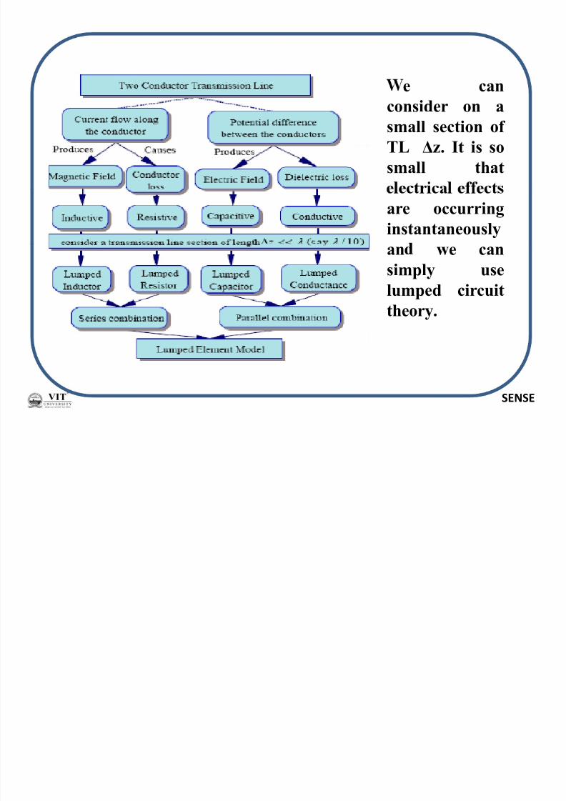
e can

consider on a

small section of

TL ∆

z. It is sosmall that

are occurring

instantaneouslyan we can

simply use

lumped circuit

theory.

SENSE



I

+ + + +

I + I I H

I + I

na ys s L j R ω +),( t z I

dI I δ +

V

I - - - -

V + V

I + I

V

I H

V + V

I + I

dz

),( t zV C jG ω +dz

dV zV δ +

From Kirchoff Volta e Law Kirchoff current law

zdt

dV C zGV z

dz

dI I I δ δ δ +=⎟

⎠

⎞⎜⎝

⎛ +− zdt

dI L z RI z

dz

dV V V δ δ δ +=⎟

⎠

⎞⎜⎝

⎛ +−

zdt

dI L z RI z

dz

dV δ δ δ +=− z

dt

dV C zGV z

dz

dI δ δ δ +=−

dt

dI L RI

dz

dV +=−

dt

dV C GV

dz

dI +=−(a) (b)



dI

Let’s V=Voe jωt , I = Ioe

jωt

Therefore

V j

dt

ω =dt

=en

( ) I L j Rdz

dV ω +=− ( )V C jG

dz

dI ω +=−

a

b

Differentiate with respect to z

( )dI

L j RV d

ω +=−2

2 ( )dz

dV C jG

dz

I d ω +=−

2

2

z z( )( )V C jG L j R

dz

V d ω ω ++=

2

2

( )( ) I C jG L j Rdz

I d ω ω ++=

2

2

V

dz

V d 2

2 γ = I

dz

I d 2

2

2

γ =



The solution of V and I can be written in the form of

c d z z Be AeV γ γ +− +=o

z z

Z Be Ae I

γ γ +−

−=

where

⎥⎦

⎤

⎢⎣

⎡

+

+=

C jG

L j R Z

o ω

ω

( )( )C jG L j R j ω ω β α γ ++=+=and

Let say at z=0 , V=VL , I=IL and Z=ZL

ef

B AV L +=o

L Z

B A I −=

and L

L

L Z

I

=



o L L Z I V A

+=

o L L Z I V B

−=

Inserting in equations ( c) and (d) we have

⎥⎥⎤

⎢⎢⎡ −

−⎥⎥⎤

⎢⎢⎡ +

=−+−+

22)(

z z

o L

z z

L

ee Z I

eeV zV

γ γ γ γ

⎥⎤

⎢⎡ −

−⎥⎤

⎢⎡ +

=−+−+

)( z z

L z z

L

eeV ee I z I

γ γ γ γ

o



⎤⎡ + − z zee

γ γ ⎤⎡ − − z zee

γ γ

⎥⎦⎢⎣

=

2

cos zγ u

⎥⎦⎢⎣ 2

Then we have

)sinh()cosh()( z Z I zV zV o L L

γ γ −= *

)sinh()cosh()( z Z

V z I z I

o

L L γ γ −= **

⎟⎟

⎜⎜

−

−==)sinh()cosh(

)sinh()cosh(

)(

)()(

zV

z I

z Z I zV

z I

zV z Z

L L

o L L

γ γ

γ γ and

o



⎟⎟ ⎠⎜⎜⎝ −−

= )sinh()cosh(

)sinh()cosh(

)( z Z z Z

z Z z Z

Z z Z Lo

o Lo γ γ

γ γ or

⎟⎟

⎠

⎜⎜

⎝

⎛

−

−=

)tanh(

)tanh()(

z Z Z

z Z Z Z z Z

Lo

o Lo

γ

γ Or further reduce

For lossless transmission line , γ= jβ since α=0

⎟⎟ ⎞

⎜⎜⎛ +

= )tan(

)( z jZ Z

Z z Z o Lo

β )cos()cosh( z z j β β =

sinsinh −=o



Standin Wave Ratio SWRantinode

node z

Beγ

Reflection coefficient

Ae-γz

Beγz

z Ae

γ −=

Γ+=+= −− 1 z z ze Be AeV γ γ γ

Voltage and current in term of reflection coefficient

V ⎛ Γ+1

− −− z z z Ae Be Ae

γ γ γ

o L

L I ⎠⎝ Γ−== 1

⎛ Γ+1 Z −==oo

L Z Z ⎠⎝ Γ−

=1o Z



For loss-less transmission line γ = jβ

By substituting in * and ** ,voltage and current amplitude are

2/12 gcos +++= z zV

2/1

2 )2cos(21)( θ β +Γ−Γ+= z A z I ho

Voltage at maximum and minimum points are

max = min −=Γ+

== 1Therefore L Z

Γ−1

o Z



Other related equations

oo sZ Z I V Z =⎟⎟

⎠⎜⎜⎝

⎛

Γ− Γ+== 11

min

maxmax

s Z Z

I V Z o

o =⎟⎟ ⎠

⎜⎜⎝

⎛

Γ+ Γ−== 11

max

minmin

⎟⎟

⎞

⎜⎜

⎛ −

=Γ o L Z Z

o

From equations (g) and (h), we can find the max and min points

K,4,2,02 π π θ β ±±=+ zMaximum

K,, π π = z



Zo ZLZin

lγ tanho L jZ Z +lγ tanh Lo

on jZ Z +

o L

o L

Z Z Z Z

+−=Γ

Γ−Γ+=

1

1SWR



Various forms of Transmission Lines

Two wire

cable Coaxialcable

Microstripe

line

Rectangular

waveguideCircular

waveguideStripline



Comparison of Waveguide and Transmission Line Characteristics

Transmission line

• -

wire, coaxial, microstrip, etc.).• Normal operating mode is the TEM or quasi-TEM mode (can support

.

• No cutoff frequency for the TEM mode. Transmission lines can

transmit signals from DC up to high frequency.• gn can s gna a enua on a g requenc es ue o con uc or

and dielectric losses.

• Small cross-section transmission lines (like coaxial cables) can only

ransm ow power eve s ue o e re a ve y g e s concen ra eat specific locations within the device (field levels are limited by

dielectric breakdown).

arge cross-sec on ransm ss on nes e power ransm ss on nes

can transmit high power levels.



Comparison of Waveguide and Transmission Line Characteristics

Waveguide

• Metal waveguides are typically one enclosed conductor filled with an

,

consists of multiple dielectrics.

pera ng mo es are or mo es canno suppor a mo e .

• Must operate the waveguide at a frequency above the respective TE orTM mode cutoff frequency for that mode to propagate.

• Lower signal attenuation at high frequencies than transmission lines.

• Metal waveguides can transmit high power levels. The fields of thepropagating wave are spread more uniformly over a larger cross-

sectional area than the small cross-section transmission line.

• Large cross-section (low frequency) waveguides are impractical due to

large size and high cost.



SENSE



( )ab L /ln2π

µ

=a

ab

C

/ln

2 ε π = c

c

ck

f =( )ab Z o /ln

2

1

ε

µ

π =

r

k c = 2

Where a = radius of inner conductor

b = radius of outer conductor

FALLSEM2013-14_CP1630_24-Jul-2013_RM01_L5-L5_FS-2013-14-review-of-TL

Documents

Transcript of FALLSEM2013-14_CP1630_24-Jul-2013_RM01_L5-L5_FS-2013-14-review-of-TL