Fail-Stop Failure ABFT for CholeskyDecomposition

Doug Hakkarinen, Student Member, IEEE , Panruo Wu, StudentMember, IEEE , and Zizhong Chen, Senior Member, IEEE

Abstract—Modeling and analysis of large scale scientific systems often use linear least squares regression, frequently employingCholesky factorization to solve the resulting set of linear equations. With large matrices, this often will be performed in highperformance clusters containing many processors. Assuming a constant failure rate per processor, the probability of a failureoccurring during the execution increases linearly with additional processors. Fault tolerant methods attempt to reduce theexpected execution time by allowing recovery from failure. This paper presents an analysis and implementation of a faulttolerant Cholesky factorization algorithm that does not require checkpointing for recovery from fail-stop failures. Rather, thisalgorithm uses redundant data added in an additional set of processes. This differs from previous works with algorithmic methodsas it addresses fail-stop failures rather than fail-continue cases. The implementation and experimentation using ScaLAPACKdemonstrates that this method has decreasing overhead in relation to overall runtime as the matrix size increases, and thusshows promise to reduce the expected runtime for Cholesky factorizations on very large matrices.

Index Terms—Extreme scale systems, Linear Algebra, Checkpoint Free, Algorithm Based Fault Tolerance.

F

1 INTRODUCTION

In scientific computing, the manipulation of largematrices is often used in the modeling and analysisof large scale systems. One such method widely usedacross many applications is linear regression. Linearregression tries to find the combination of M coeffi-cients for M regressors that best fit a model based ondata of R samples, with each sample consisting of aset of independent variables (xi) and a resulting value(yi, with the set of yi called y). Then a matrix X iscreated, where each row contains the regressor valuesfrom a sample. Regressors can be constants (for anintercept), or functions of the independent variables.Most often linear regression is used to find the bestestimate in the presence of a random unknown error.Usually this estimation is done as an overdeterminedsystem, meaning there are more samples than coeffi-cients. Thus, X is of dimension R×M , with R largerthan M . The problem takes the form of finding thebest set of coefficients for the regressors (commonlyβ) such that Xβ has the minimal difference from y.In ordinary least squares regression, this problem isdefined as finding β such that XTXβ=XTy. The firststep is to compute the matrix product of the of XTX.The resulting M ×M matrix, A, is symmetric positivesemi-definite and often symmetric positive definite.Factoring this matrix into a triangular form for opti-mization is often desirable and produces an efficient

Doug Hakkarinen is with the Department of Electrical Engineeringand Computer Science, Colorado School of Mines, Golden CO. Email:dhakkari@mines.eduPanruo Wu and Zizhong Chen are with the Department of Com-puter Science and Engineering,University of California, Riverside. Email:pwu011,chen@cs.ucr.edu

way to find optimal coefficients through substitution.As such, factoring a symmetric positive definite isfocused on through several techniques.

One efficient method for factoring a symmetricpositive semi-definite matrix is through Cholesky fac-torization. In this factorization method, the result iseither the upper triangular matrix U, such that UTUis A, or the lower triangular matrix X, such thatXXT is A. In this work we focus only on creatingthe lower factorization L, although all methods thatare used for X can be done for U as well since itis a symmetric algorithm. The Cholesky method isfavored for many reasons, the foremost being it isnumerically stable and does not require pivoting. Thesequential Cholesky algorithm has several forms, suchas the Outer Product, Right-Looking, and bordered.

In order to use Cholesky factorization for large datasets, methods need to be used that take into accountthe effects of performance based on cache usage. Thelibraries LAPACK and BLAS aid in optimizing theusage of cache through the blocking technique. Theimpact of this technique on the Cholesky method isthat more than one iteration is effectively handled atonce. Specifically, the number of iterations handledat once is the block size, MB. Blocking reduces se-quential iterations (row by row) into fewer blockediterations. The advantage of the blocked approachthat many of the steps use the same data. Taking theactions across the entire row will clear the cache ofthis data, causing additional cache misses. Blockingprevents taking the action across the entire row, thusimproving the performance.

If using a single node is not fast enough or thematrix size exceeds the memory on a single node,

DRAFT: IEEE TRANSACTIONS ON PARALLEL AND DISTRIBUTED SYSTEMS 2

multiple process methods have been explored, partic-ularly in the widely known software ScaLAPACK [9].ScaLAPACK combines both the usage of LAPACKblocked techniques and support for multiple pro-cesses. Since there are more processes and there isan advantage to distributing the work across manyprocesses, ScaLAPACK uses block-cyclic matrix dis-tribution of data. In block-cyclic matrix distribution,the blocks that a particular processor contains comefrom many parts of the global matrix. As such, addi-tional consideration must be taken when developingalgorithms that act with ScaLAPACK and also interactwith the data on the processes directly.

As the number of processors employed grows large,the probability of a failure occurring on at least oneprocessor increases. In particular, a single processorfailure is commonly modeled using the exponentialdistribution during periods of constant failure rates.Constant failure rates appear in the “Normal life” or“random failure” period in the commonly referencedBathtub curve [20]. Constant failure rates apply forprocessors that are beyond their burn-in phase andnot yet to their end of life phase. Under the assump-tion of an exponential failure rate of each processor,the failure rate of the overall system can be shown togrow linearly with the number of processors. Thus,for systems with increasing numbers of processors,failures become a larger problem. As the high perfor-mance community looks to exa-scale processing thefailure rates must be addressed.

In order to counteract this increasing failure rate assystems grow, many techniques [14], [15] have beendeveloped in order to provide fault tolerance. Themost traditional technique is the checkpoint, or theroutine saving of state. Some research has suggestedthat checkpointing approaches may face further diffi-culties as the number of processes expands [13].

Another promising approach is to take advantageof additional data held within the algorithm beingexecuted to allow the recovery of a failed process. Ap-proaches are known as algorithm based fault tolerance(ABFT) [19], [4], which use information at the end ofexecution of an algorithm to detect and recover fail-ures and incorrect calculations. ABFT has tradition-ally been developed for fail-continue failures (failureswhich do not halt execution), with the goal of detect-ing and correcting errors at the end of computation.ABFT algorithms have received wide investigation,including development for specific hardware architec-tures [3], efficient codes for use in ABFT [2], [27],comparisons to other methods [26], [25], and analysisof potential performance under more advanced failureconditions [1]. The use of result checking in contrastto ABFT post-computation has also been studied [24].Building on earlier work [17], we investigate the useof algorithmic methods to help recover fail-stop fail-ures, or failures that halt execution. More importantly,our work demonstrates that ABFT can be used to

recover failures during computation, rather than onlyafter computation completes. Similar ABFT methodsfor fail-stop failures have been studied for matrixmultiplication [7], [8], [5], for LU Decomposition [10],[11], [12], and Conjugate Gradient methods [22]. Thismethod is not an endpoint, as potential improvementscan be made through hot-replace strategies [28], [29],[30], but those methods depend on the algorithm tomaintaining a checksum (such as is demonstrated inthis work).

The differences between using data from within analgorithm versus checkpointing are numerous. Themost specific difference is that the algorithm, for themost part, runs with little modification or stoppagesuch as is required to perform a checkpoint. If theamount of time to recover is approximately constantrelative to the overall execution time, then this greatlyimproves the recovery time. The disadvantage ofalgorithmic recovery is that it only works on thealgorithm in question, whereas checkpointing canoften work regardless of what computation is beingperformed. Furthermore, depending on the algorithmand the recovery method, it may require more intensecomputation time to determine and restore the stateof a failed process, which may or may not exist incheckpointing systems. In this work, we develop theuse of algorithmic recovery for single fail-stop failuresduring a Cholesky factorization. While we only exam-ine the case of a single failed process, adaptation forrecovery of multiple failures is certainly possible [6].

2 CHOLESKY FACTORIZATION WITHCHECKSUM MATRICES

In this section, we explore the impact of checksum ma-trix inputs (as defined by [19]) on different Choleskyfactorization algorithms. Checksum matricies of thistype introduce redundant data as additional columnsas linear combinations of the original matrix columns.Cholesky factorization requires a positive definite ma-trix input. As the checksum matrix is not linearly in-dependent, it is no longer invertible, and not positivedefinite. Therefore, care must be taken to ensure theCholesky factorization result to match the result offactorization of the original matrix. We explore the ef-fects of checksum matrices on the Bordered algorithm,

Af =

a1,1 a1,2 · · · a1,n∑n

1 a1,ja2,1 a2,2 · · · a2,n

∑n1 a2,j

.... . . . . . . . .

...an,1 an,2 . . . an,n

∑n1 an,j∑n

1 ai,1∑n

1 ai,2 · · · ∑n1 ai,n

∑n1

∑n1 ai,j

Fig. 1. Diagram of an unblocked checksum matrix. ForCholesky, the original matrix (without the checksum)must be symmetric (aij = aji) and positive definite.

DRAFT: IEEE TRANSACTIONS ON PARALLEL AND DISTRIBUTED SYSTEMS 3

1: for i = 1 :M do2: A(i, 1 : i − 1) ← A(i, 1 : i − 1)L(1 : i − 1, 1 :

i− 1)−1 {where L(1 : i− 1, 1 : i− 1) is the lowertriangular part of A(1 : i− 1, 1 : i− 1) includingmain diagonal. }

3: A(i, i)←√A(i, i)

4: end for

Fig. 2. The unblocked bordered Cholesky algorithmfactorizes a M ×M symmetric matrix into A = LLT in-place, where the lower triangular matrix L overwritingthe lower triangular part of A.

the Outer Product algorithm, and the Right-Lookingalgorithm.

We establish which Cholesky algorithm variantshave the possibility of maintaining a checksum duringcomputation. An example unprocessed, unblockedchecksum matrix is shown in Figure 1. This checksummatrix is the starting point for all the unblockedalgorithms being examined. For the algorithms thatthe checksum is maintainable, we then establish howto do so in a 2-D block cyclic version.

2.1 The Bordered Algorithm Does Not MaintainChecksums During Computation

The sequential, unblocked inline Bordered algorithmprocesses the matrix from upper left corner to thelower right corner. We focus on the generation ofthe L matrix (lower triangle), but symmetry holds forthe upper triangular matrix. In each iteration of theBordered algorithm, one additional row of entries isprocessed on and below the diagonal.

Figure 2 shows the algorithm. If this algorithm isperformed on the checksum matrix in the Figure 1,the checksum row and checksum column (the last rowand column) will not be touched until the last itera-tion. Updating the payload matrix without touchingthe checksums accordingly will therefore invalidatethe checksums during the whole factorization. It canbe shown that the checksum becomes valid only aftern iterations, at which point the desired factorizationis done. The checksums are not naturally maintainedduring the factorization.

2.2 The Outer Product Algorithm MaintainsChecksums

The sequential, unblocked Cholesky Outer Productmethod can be separated into iterations for which Miterations as shown in Figure 3. This method is calledthe Outer Product method [16].

The first modification of the Outer Product algo-rithm is to initially form the checksum matrix usinga summing reduce operation to the checksum pro-cess row and column (see Figure 1). If the originalmatrix is n × n, the unblocked checksum matrix is

1: for i = 1 :M do2: A(i :M, i)← A(i :M, i)/

√A(i, i)

3: if i < M then4: A(i + 1 : M, i + 1 : M) ← A(i + 1 : M, i + 1 :

M)−A(i+ 1 :M, i)A(i+ 1 :M, i)T

5: end if6: end for

Fig. 3. The unblocked outer-product Cholesky al-gorithm factorizes a M × M symmetric matrix intoA = LLT in-place, where the lower triangular matrixL overwriting the lower triangular part of A.

(n + 1) × (n + 1). The second modification is thatwe skip the last iteration since the checksum matrixis not positive definite anymore. Now perform thealgorithm described in Figure 3 on the augmentedchecksum matrix. We claim that every iteration i inFigure 3 preserves the checksums in some way. Thealgorithm stops after n iterations, and the columnchecksums are maintained after every iteration of theunblocked, inline Outer Product algorithm.

To see why the outer product algorithm maintainsthe column checksums at the end of every iteration,we need only to look at the operations in one iterationin Figure 3. For brevity we denote the sub matrix A(i :n, i : n) by Ai:n,i:n. Note that now M = n+ 1. We useinduction on i. Suppose before any iteration i, the firsti− 1 columns in the lower triangular L, have columnchecksums available at the checksum row:

An+1,j =

n∑

k=j

Ak,j , j = 1, . . . , i− 1 (1)

and the trailing matrix has column checksum avail-able:

An+1,j =

n∑

k=i

Ak,j , j = i, . . . , n (2)

These conditions hold when i = 1 by construction ofthe checksum matrix. We show that upon completionof iteration i, the conditions (1, 2) hold for i + 1. Infact, after the line 2 in Fig 3, the condition (1) holdsfor j = i since the vector and its checksum are scaledby the same factor. After the trailing matrix update inline 3

Ai+1:n+1,i+1:n+1 ← Ai+1:n+1,i+1:n+1−Ai+1:n+1,iATi+1:n+1,i

we would like to prove that condition (2) holds fori+1. In fact, the trailing matrix update is logically asthe following equation if both line 2 and 4 in Fig 3are not done in-place in memory:

Bi:n+1,i:n+1 ← Ai:n+1,i:n+1−1√Ai,i

Ai:n+1,i1√Ai,i

ATi:n+1,i

Note that the checksum property is closed undermatrix multiplication (column checksum matrix mul-tiply by row checksum matrix) and addition. It is

DRAFT: IEEE TRANSACTIONS ON PARALLEL AND DISTRIBUTED SYSTEMS 4

0BBBBBBBBBBBBBBB@

a1,1pa1,1

0 · · · 0 0

a2,1pa1,1

a2,2 �a2,1a2,1

a1,1· · · a2,n �

an,1a2,1

a1,1

nX

1

ai,2 �a2,1

a1,1

nX

1

ai,1

.... . .

. . .. . .

...

an,1pa1,1

an,2 �a2,1an,1

a1,1. . . an,n �

an,1an,1

a1,1

nX

1

ai,n �an,1

a1,1

nX

1

ai,1

Pn1 ai,1pa1,1

nX

1

ai,2 �a2,1

a1,1

nX

1

ai,1 · · ·nX

1

ai,n �an,1

a1,1

nX

1

ai,1

nX

1

nX

1

ai,j �(Pn

1 ai,1)2

a1,1

1CCCCCCCCCCCCCCCA

Fig. 4. Unblocked checksum matrix after one iterationof the unblocked, inline outer product method. Thefirst column contains elements of L. Columns 2 ton+ 1 are the updated but not yet processed elements.The top row are all zero. The column checksums arepreserved.

easy to see that Bi:n+1,i:n+1 is the difference betweentwo full checksum matrix therefore must also bea full checksum matrix. Further, we note that thefirst row Bi,i+1:n+1 = 0, which means that the non-zero sub matrix Bi+1:n+1,i+1:n+1 is a full checksummatrix. We conclude by noting that this sub matrix isthe new value of Ai+1:n+1,i+1:n+1. Hence, inductionshows that condition (1, 2) holds after every iterationi = 1, 2, . . . , n. Figure 4 shows the preserved columnchecksums at the end of the first iteration.

In summary, after each iteration, both the check-sums of the first i columns and the south-east (n−i)×(n − i) trailing matrix maintain checksums naturally.The equivalent of a process failure in the unblockedalgorithm would be the erasure of a particular ele-ment in the matrix. In order to recover any elementin the matrix, the checksum along with the otherelements could be used at any step. For example,element Ar,c is reconstructed by

Ar,c ← AM+1,j − (

r−1∑

k=1

Ak,c +

M∑

k=r+1

)Ak,c

The sum of the other rows in its column recovers thechecksum row.

2.3 Right-Looking Cholesky Algorithm MaintainsColumn ChecksumsThe Right-Looking inline, unblocked algorithm is sim-ilar to the inline, unblocked Outer Product algorithm.The key difference between the Right-Looking algo-rithm and the Outer Product algorithm is the datathat is maintained. Computationally speaking, sincethe trailing matrix B is symmetric there is no needto maintain the entire submatrix. It is possible tocompute half of the B matrix at the same time thatthe L matrix is being filled in. The Right-Looking al-gorithm utilizes the symmetry and does not maintainthe unneeded half of the matrix.

The result of these optimizations in the Right-Looking algorithm is that the columns that containB no longer add up to the checksum. The elementsabove the diagonal in the B matrix can no longer

Fig. 5. Unblocked Right-Looking algorithm recovery.Yellow lines indicate what elements add to checksumfor columns where the column for recovery is lessthan or equal to the iteration. Purple indicates whatelements are needed for recovery when the column forrecovery is greater than the iteration number.

be used to recover a missing value. For a failurein column c, the missing elements are contained inrow c. Figure 5 demonstrates how to recover withoutadditional steps in each iteration.

The checksum row, along with the other elementsof the matrix of the unblocked, inline Right-Lookingmethod, contains sufficient information to recover anysingle element in the lower triangle of the matrix. Weexamine the block cyclic version of this algorithm inSection 3.2.

2.4 Summary of Checksum MaintenanceA summary of the checksums maintained by eachalgorithm is shown in Table 1. The Bordered algorithmis unable to maintain either row or column checksum.The Outer Product algorithm is able to 1) maintainboth Row and Column Checksums for the as yetunprocessed matrix, 2) column checksums for the Lmatrix, and, 3) can maintain row redundancy for theL matrix (with modification). The Right-Looking al-gorithm maintains the column checksum, but requiresan additional step for recovery in order to re-establishsymmetry in the matrix. As both the Right-Lookingalgorithm and Outer Product algorithm can recoverfrom a failure, we now look at how these algorithmsbehave in a 2-D block cyclic data distribution.

Bordered Outer Product Right-LookingNo Y es Y es∗

TABLE 1Column checksums maintain or not?

3 2D BLOCK CYCLIC CHOLESKY ALGO-RITHMS WITH CHECKSUMS

In blocked Cholesky algorithms, including block-cyclic algorithms, a block is processed each iteration.

DRAFT: IEEE TRANSACTIONS ON PARALLEL AND DISTRIBUTED SYSTEMS 5

a

b B

bT

Fig. 6. Blocked Outer Product Cholesky factorization,in iteration 3

1: while a is not empty do2: (POTF2) Solve L from a = LLT , a← L3: (TRSM) Solve X from b = XaT , b← X4: (SYRK) B ← B − bbT5: Move to the trailing matrix:

(a bT

b B

)← B

6: end while

Fig. 7. Blocked Outer Produce Cholesky factorizationalgorithm.

For example, in the blocked Outer Product algorithm,several diagonal elements are handled on each iter-ation. When distributing a blocked algorithm acrossa process grid, each process generally manipulatesonly one block at a time. Blocks are usually sized tomaximize the benefit of cache. In a block cyclic datadistribution, each process has more than one block ofdata, with each block having a specific size (definedas MB rows and NB columns). Additionally, blocksfrom different parts of the matrix are on each process.These blocks are assigned from the global matrix tothe processes in a cyclic fashion [21] to balance load.Basically the matrix is divided into many blocks, andthe processes are treated as a p1× p2 2D process grid.The blocks are assigned to the processes in the processgrid in a round-robin manner. More specifically, block(i, j) got assigned to processer (i mod p1, j mod p2)assuming all indices start from 0.

For simplicity, we cover the case where the proces-sor grid, without the checksum row and column, issquare P×P . Additionally, we assume the blocking issquare (i.e., MB×MB). As the input matrix (withoutchecksum) is M ×M , and there are P ×P processors(without checksum processor), we assume each pro-cessor holds an equal number of elements,M

2

P 2 , whichwe assume is a square number of elements with aside length ML. Finally, for ease of implementation,we assume each processor’s local matrix to be evenlydivisible into a square number of blocks on eachprocessor (i.e., (ML)2 mod (MB)2 = 0).

While these assumptions greatly ease the imple-mentation, this method can still be used for Cholesky

factorizations where these conditions do not hold.Block cyclic checksum algorithms function by reserv-ing an extra row and/or column of processes tohold a checksum of the values, which is called thechecksum process row and checksum process column,respectively. We call a matrix with a checksum processrow as a row process checksum matrix. Note that insuch a matrix, each process column has respectiveblocks that sum to the value in the checksum processrow. We call a matrix with both checksum process rowand column a full process checksum matrix. In thechecksum processes, a sum of the respective values ofthe other blocks in the same row or column, respec-tively, are kept. To do so, each checksum process holdsthe same number of elements as any other process,namely MXLLDA2. The total number of additionalprocesses to add a checksum row and column is2P + 1. The full process checksum matrix thereforeis (M +MXLLDA)× (M +MXLLDA).

The execution of the block cyclic Cholesky withchecksum routine proceeds just as a normal block-cyclic Cholesky routine with the following exception:every P iterations, when a checksum block would bethe next block to be used as the matrix diagonal, thealgorithm jumps to the next iteration. As such, noadditional iterations are performed in the running ofthe Cholesky routine. However, each iteration maytake longer due to the additional communication andtime due to the existence of the checksum row andcolumn. Other than this, the checksum block cyclicCholesky algorithms function similarly to a standardblock cyclic Cholesky algorithm, such as is found inScaLAPACK’s PDPOTRF.

3.1 The 2D Block Cyclic Outer Product Algorithm

For a distributed 2-D block cyclic distribution, theblocked version is effectively the same. The majordifference is that care must be taken in order to ensurethat the data needed at any step is sent to the correct

(a) Global view (b) Local view

Fig. 8. Global and Local views of a 6x6 input matrix(8x8 checksum matrix), symmetric blocked checksummatrix to be used in demonstration of the 2-D blockcyclic Outer Product and Right-Looking algorithms.The size of each block is 1 element, the number ofblocks per process is 4 (MB = 2).

DRAFT: IEEE TRANSACTIONS ON PARALLEL AND DISTRIBUTED SYSTEMS 6

(a) Global view (b) Local view

Fig. 9. Global and local views after three iterations ofthe Outer Product algorithm. Blue is the unprocessedmatrix. Green are parts of L. Orange are parts thatshould be treated as 0s for ease of using columnchecksums. The next step would have a checksumblock as the diagonal block, so it is skipped. The nowzero checksum blocks are noted in yellow.

processes. The snapshot of iteration j = 3 is shownin Figure 6 and the blocked right looking Choleskysalgorithm is shown in Figure 7.

For clarity, we present a numerical example of theblocked version. The initial checksum matrix is shownin Figure 8. Figure 9 illustrates the state after the firstthree steps. From this view, it looks similar to theunblocked method as the block sizes are 1; however,note that the checksums are maintained within eachsection of the matrix. After step three, the next stepwould have a checksum block as the diagonal blockand is skipped. As the data of the original matrix isin the non-checksum blocks, the algorithm producesthe same result as the non-checksummed algorithm.

3.2 Handling Failure in a 2D Block Cyclic Right-Looking Algorithm

We next look at the 2-D block cyclic Right-Lookingalgorithm. This algorithm is similar to the correspond-ing Outer Product algorithm. Only the lower triangleof B matrix is maintained.

After any given iteration of the inline algorithm,the global matrix contains three different parts: 1) thepartial result matrix L, 2) the unfactorized elements B,and 3) data that is no longer needed. Figure 10 showsthe breakdown of a matrix after one iteration. The Lportion of the matrix holds the partial result. The Bmatrix contains the yet to be factorized elements.

For blocks that are in the L section of the matrix,the checksum is the sum of the entire column ofcorresponding local entries of L. For blocs in the Bsection of the matrix, the checksum is the sum of theelements in the column of the B matrix, includingthose that would be past the diagonal if they weremaintained. To use these checksum blocks, symmetricelements must be used to recover elements in B sim-ilar to the unblocked Right-Looking algorithm. Theseare transposed from the equivalent row of the failure

(a) Global view (b) Local view

Fig. 10. Global and Local views of Matrix from Figure 8after one iteration of the Right-Looking algorithm. Theblock size is 1 element. Green shows parts of L. Blueshows unprocessed data in B. Red shows parts of Bthat are not maintained.

Recovery Routine1: Restore Matrix Symmetry for Column fc2: A(fr, fc, ∗)← 03: if Column = fc then4: for all Blocks b ∈ LocalMatrix do5: if fr = checksumr then6: Reducecol

∑Pi=1A(i, fc) to A(fr, fc)

7: else8: Reducecol A(P + 1, fc) +∑P

i=1−A(i, fc) to A(fr, fc)9: end if

10: end for11: end if

Fig. 11. The steps to recover from a failure in the 2-D block cyclic Right-Looking parallel algorithm, whereA(r,c,b) is the local matrix block for row r, column c,block b, the process failure row is fr and the processfailure column is fc.

column into the failure column, thus reconstructingthe column checksum relationship.

In a block cyclic distribution, one process maycontain data from all three sections. Thus, upon afailure, each element must be examined individuallyto determine how it should be recovered and restoresymmetry as necessary. Once in this form, the blockcyclic equivalent of the unblocked recovery algorithmis used (see Figure 11).

When a failure occurs, the algorithm must restorethe values of the failed data to the failed process.The following preconditions must be met: 1) the rowand column of the failed process must be known,2) no additional processes may fail during recovery,3) the failed step of the iteration must be knownand detected before the next step begins, and 4) theiteration must be known. Section 4.3 examines specificrecovery procedures based on the step in an iterationwhen a process fails.

DRAFT: IEEE TRANSACTIONS ON PARALLEL AND DISTRIBUTED SYSTEMS 7

4 OVERHEAD SCALABILITY ANALYSIS

To examine the overhead scalability of ABFTCholesky, we first examine the runtime of the (non-fault tolerant) blocked Right-Looking Cholesky fac-torization on a P × P process grid. We then examinethe scalability of the overhead and for recovery in asquare ((P + 1) × (P + 1)) process grid using a fullprocess checksum matrix.

4.1 Blocked Right-Looking Cholesky Runtime

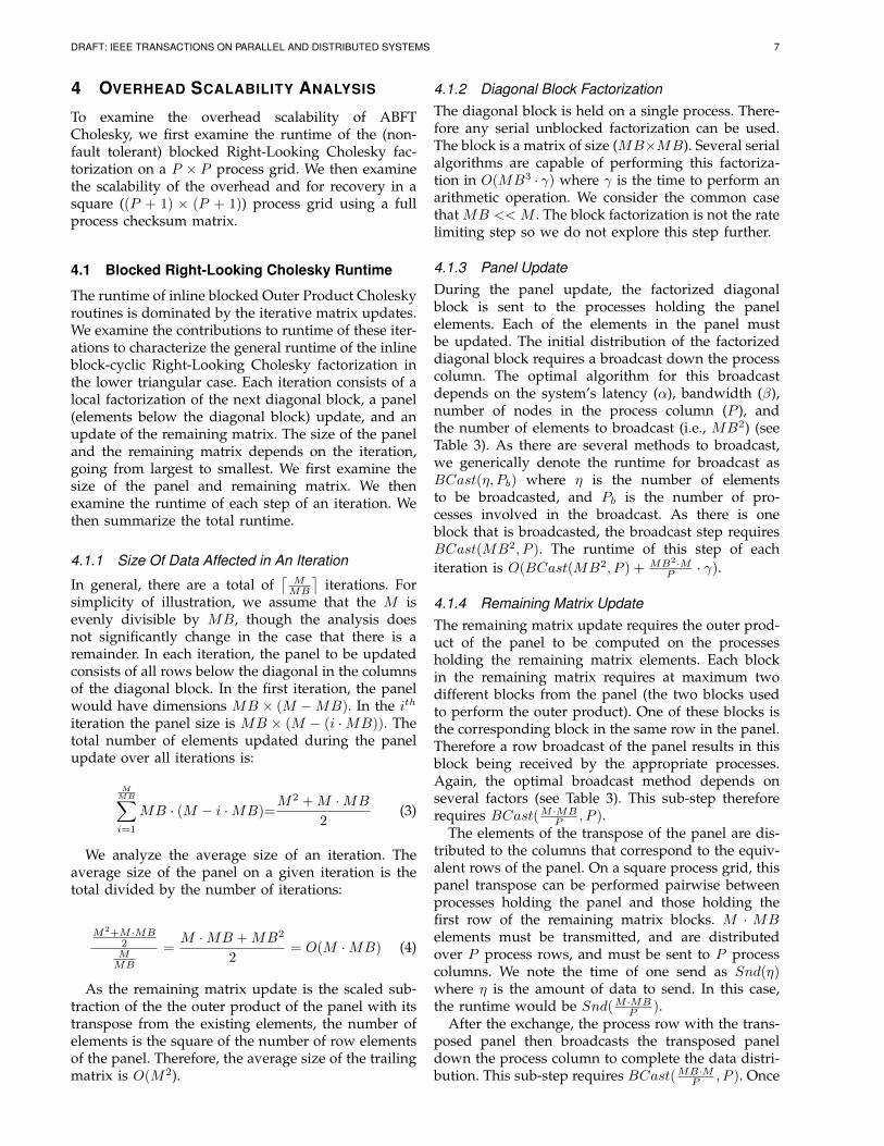
The runtime of inline blocked Outer Product Choleskyroutines is dominated by the iterative matrix updates.We examine the contributions to runtime of these iter-ations to characterize the general runtime of the inlineblock-cyclic Right-Looking Cholesky factorization inthe lower triangular case. Each iteration consists of alocal factorization of the next diagonal block, a panel(elements below the diagonal block) update, and anupdate of the remaining matrix. The size of the paneland the remaining matrix depends on the iteration,going from largest to smallest. We first examine thesize of the panel and remaining matrix. We thenexamine the runtime of each step of an iteration. Wethen summarize the total runtime.

4.1.1 Size Of Data Affected in An Iteration

In general, there are a total of⌈MMB

⌉iterations. For

simplicity of illustration, we assume that the M isevenly divisible by MB, though the analysis doesnot significantly change in the case that there is aremainder. In each iteration, the panel to be updatedconsists of all rows below the diagonal in the columnsof the diagonal block. In the first iteration, the panelwould have dimensions MB × (M −MB). In the ith

iteration the panel size is MB × (M − (i ·MB)). Thetotal number of elements updated during the panelupdate over all iterations is:

MMB∑

i=1

MB · (M − i ·MB)=M2 +M ·MB

2(3)

We analyze the average size of an iteration. Theaverage size of the panel on a given iteration is thetotal divided by the number of iterations:

M2+M ·MB2MMB

=M ·MB +MB2

2= O(M ·MB) (4)

As the remaining matrix update is the scaled sub-traction of the the outer product of the panel with itstranspose from the existing elements, the number ofelements is the square of the number of row elementsof the panel. Therefore, the average size of the trailingmatrix is O(M2).

4.1.2 Diagonal Block FactorizationThe diagonal block is held on a single process. There-fore any serial unblocked factorization can be used.The block is a matrix of size (MB×MB). Several serialalgorithms are capable of performing this factoriza-tion in O(MB3 · γ) where γ is the time to perform anarithmetic operation. We consider the common casethat MB << M . The block factorization is not the ratelimiting step so we do not explore this step further.

4.1.3 Panel UpdateDuring the panel update, the factorized diagonalblock is sent to the processes holding the panelelements. Each of the elements in the panel mustbe updated. The initial distribution of the factorizeddiagonal block requires a broadcast down the processcolumn. The optimal algorithm for this broadcastdepends on the system’s latency (α), bandwidth (β),number of nodes in the process column (P ), andthe number of elements to broadcast (i.e., MB2) (seeTable 3). As there are several methods to broadcast,we generically denote the runtime for broadcast asBCast(η, Pb) where η is the number of elementsto be broadcasted, and Pb is the number of pro-cesses involved in the broadcast. As there is oneblock that is broadcasted, the broadcast step requiresBCast(MB2, P ). The runtime of this step of eachiteration is O(BCast(MB2, P ) + MB2·M

P · γ).

4.1.4 Remaining Matrix UpdateThe remaining matrix update requires the outer prod-uct of the panel to be computed on the processesholding the remaining matrix elements. Each blockin the remaining matrix requires at maximum twodifferent blocks from the panel (the two blocks usedto perform the outer product). One of these blocks isthe corresponding block in the same row in the panel.Therefore a row broadcast of the panel results in thisblock being received by the appropriate processes.Again, the optimal broadcast method depends onseveral factors (see Table 3). This sub-step thereforerequires BCast(M ·MB

P , P ).The elements of the transpose of the panel are dis-

tributed to the columns that correspond to the equiv-alent rows of the panel. On a square process grid, thispanel transpose can be performed pairwise betweenprocesses holding the panel and those holding thefirst row of the remaining matrix blocks. M · MBelements must be transmitted, and are distributedover P process rows, and must be sent to P processcolumns. We note the time of one send as Snd(η)where η is the amount of data to send. In this case,the runtime would be Snd(M ·MB

P ).After the exchange, the process row with the trans-

posed panel then broadcasts the transposed paneldown the process column to complete the data distri-bution. This sub-step requires BCast(MB·M

P , P ). Once

DRAFT: IEEE TRANSACTIONS ON PARALLEL AND DISTRIBUTED SYSTEMS 8

the data is distributed, there are O(M2) elements toupdate using P×P processes. As each element updaterequires MB multiplications, MB additions and onesubtraction, the element update is O(MB·M2

P 2 · γ) eachiteration. The update step therefore has a runtime of:

O(BCast(M ·MB

P,P )+Snd(

M ·MB

P)+M2·MBγ

P 2)

(5)

4.1.5 Runtime Over IterationsThe overall runtime can be approximated as the av-erage time of each step multiplied by the number ofiterations. The maximum in this case is determinedeither by the time to broadcast, or the arithmeticupdate of any given iteration. In both cases, the re-maining matrix update dominates the iteration. Thereare M

MB iterations. The overall runtime for the dis-tributed block-cyclic Cholesky factorization throughthis variant is therefore:

O(M3γ

P 2+M ·BCast(MB·M

P ,P )+BCast(MB·MP ,P )

MB)

(6)

4.2 Overhead of ABFT Cholesky on a Square Gridwith Full Processor Checksum MatrixThe overhead of ABFT Cholesky consists of the over-head for setting up the initial checksum process rowand checksum process column (i.e., full checksummatrix), the overhead due to increased matrix size,and the overhead due to algorithm modification. Theoverhead of the algorithm modification is negligibleas it consists only of skipping iterations where achecksum block would be the diagonal block. Thischeck would only occur once per iteration. The othertwo overheads, however, deserve closer analysis. Inthis section, we assume that the original matrix isdistributed over a P × P process grid, with the fullchecksum matrix process grid being (P +1)× (P +1).

4.2.1 Overhead of Checksum Matrix SetupThe checksum process column contains a block-wisesummation of corresponding blocks over the blocks ofeach row. Therefore, each block needs to be transmit-ted and summed into the checksum process column.This operation is the equivalent of an summationMPI Reduce call. Depending on the characteristicsof the matrix and system, the best way to performthis reduction varies. As such, we note the time forreduction as Reduce(η, Pr), where η is the size of thedata to be reduced by process, and Pr is the numberof processes involved. We assume that the destinationdoes not significantly impact the runtime.

Each process, including checksum processes, holdsM2

P 2 elements. Each process row has P processes, plusthe checksum column process, making P+1 processes.

Therefore each reduction occurs over P +1 processes.As such, the reduce across rows takes Reduce(M

2

P 2 , P+1). There are a total of P reductions needed, but thesecan be done in parallel.

After construction the checksum process column,we construct the checksum process row. This con-struction is also the summation of correspondingblocks, but this time over the process columns intothe checksum process row. There are P process rows,plus the checksum row, making P + 1 rows. Again,each process holds M2

P 2 elements. The summation intothe checksum process row requires Reduce(M

2

P 2 , P +1). Once the second reduction step is complete, thechecksum process row and column setup is complete.Therefore, the overall runtime for the checksum setupstep is O(Reduce(M

2

P 2 , P + 1)).

4.2.2 Overhead of Increased Matrix SizeTo analyze the overhead of the increased matrix size,we must analyze both any increase in program wall-clock runtime and the overhead that results fromusing an increased number of processes. We first lookat the sources of increased wall-clock runtime.

The checksum matrix increases the size of the ma-trix in each dimension by one process. The modi-fied algorithm skips any iteration where a checksumblock is the diagonal block. Therefore, the numberof iterations remains

⌈MMB

⌉. Within each iteration the

amount of data has increased.In the diagonal blockfactorization step, no additional data has been intro-duced so the runtime of this step remains unchanged.During the panel update step, the diagonal blockmust be communicated to (P + 1) processes insteadof P processes and perform additional computationon the blocks held in the checksum process. For thecomputation, as an additional process is available,the amount of wall-clock time remains unchanged.The increase in the broadcast results in a runtime ofBCast(MB2, P + 1) + MB·M

P , or overhead of:

O(BCast(MB2, P + 1)−BCast(MB2, P )) (7)

During the remaining matrix update, the broad-cast across process rows and the broadcast acrossprocess columns both broadcast over one addi-tional process. Therefore these steps both now takeBCast(MB·M

P ,P+1). The panel transpose must also becommunicated from and to the respective checksumrow process of the panel and the checksum columnprocess. In a P × P grid, there is a one to onecorrespondence of these processes, and therefore thetime is only to send the elements. This is also true forthe original processes, and as such this step presentsno additional overhead. The number of matrix ele-ments that must be computed during the panel up-date also increases. However, the number of elementsincreases proportionally to the number of checksum

DRAFT: IEEE TRANSACTIONS ON PARALLEL AND DISTRIBUTED SYSTEMS 9

processes, and reside on those checksum processes.Therefore, the runtime increase for this step consistsof the increase in the additional time for broadcast, orO(BCast(MB·M

P , P + 1)−BCast(MB·MP , P )).

Looking at the iteration steps, the remaining matrixupdate dominates the runtime as in the non-faulttolerant case. As the number of iterations has notchanged, the wall-clock overhead for all the steps is:

O(M(BCast(MB·M

P ,P+1)−BCast(MB·MP ,P ))

MB) (8)

The remainder of the overhead can be classified asthe time to use the additional processors that couldbe used for some other job in a cluster. The numberof processors has increased by one processor rowand one processor column. Therefore, the numberof processors has increased from P 2 to (P + 1)2. Todetermine the overall overhead, we therefore scale thewall-clock overhead by (P+1)2

P 2 .Multiplying this overhead factor by the dominant

overhead in Equation 8 yields the approximate over-head for the fault tolerant Cholesky routine due to theincreased matrix size. Thus the overall overhead fromthe increased matrix size is:

O((P + 1)2

P 2· MMB

·BCast(MB ·MP

,P + 1)) (9)

4.3 Recovery on a P x P Processor GridWhen a process fails, the contents of its memoryrelated to the matrix need to be reconstructed whenit is restarted, or on a replacement process. We referto the process taking the place of the failed processas pf . We also assume a recovery routine is initiatedon every process that indicates which process hasfailed. With knowledge of which process failed, theother processes place pf in the equivalent point intheir communications, and that pf assumes the rolein terms of memory and processing tasks that wouldhave been performed by the failed process. Therefore,the objective of recovery is to restore the memory ofpf to a point where the factorization can continue.

Immediately after pf comes online, an arbitraryother process, say process 0, should transmit informa-tion concerning which iteration was being performed,and furthermore during what step of the iterationthe failure occurred. Additional information such asthe characteristics and decomposition of the matrixshould also be sent. Based on the iteration and thedecomposition, pf determines what block positions inthe matrix it should contain and determine whetherthose blocks contain the result matrix L, are no longerneeded (i.e., are above the diagonal in a row that hasalready been passed by the iterations), the diagonalblock Ai,i, panel blocks bi, or remaining matrix blocksBi. The other processes should likewise identify thattype of data contained in pf ’s blocks.

1: if This Node Failed then2: LocalMatrix← 03: else4: for all Blocks ∈ Local Matrix do5: if Block Above Diag AND Column = Fcol

then6: Receive Block into LocalMatrix7: Transpose LocalMatrix8: end if9: if Block Below Diag AND Row = Fcol then

10: Send LocalMatrix to transposed position11: end if12: end for13: end if14: if Column = FCol then15: if Row = ChkRow then16: ColumnReduce −ONE · LocalMatrix To

FRow17: else18: ColumnReduce LocalMatrix to FRow19: end if20: end if

Fig. 12. The steps performed by each node to recoverfrom a failure needing the Hybrid row + column data.Data is the local data matrix, Row is the processorrow, Column is the processor column, and FRow andFCo are the row and column of the failed node. Send,Receive, and ColumnReduce represent calling the re-spective MPI functions. It is assumed that a commonordering of blocks is available across processors.

For simplicity of implementation, it may also beadvantageous for any process that contains unneededblocks to ensure these blocks contain zeros as it en-ables column summation reduce calls on these blockswithout special handling of the memory for theseblocks. On the other hand, this may cause an overheadincrease and can be avoided through careful imple-mentation. pf should also ensure that the contents ofits local matrix initially are zeros.

The actions to recover any given block depends onthe type of data that should be contained in that blockand on what part of an iteration the failure occurred.Of these, there is no need to recover elements thatare no longer needed, as these blocks are not part ofeither the result nor are still needed for computation.

The most straightforward blocks to recover arethose of the resulting L matrix, as these do not dependon which step of an iteration the failure occurred. If apf is a checksum row process, any blocks in L can berecovered by performing a summation reduce call onpf ’s process column. For any other process, the blocksin L are recovered by transmitting the contents of thechecksum process of its column, and then subtractingthe result of a summation reduce of processes 1 to P(where pf contains zeros). This pattern of summation

DRAFT: IEEE TRANSACTIONS ON PARALLEL AND DISTRIBUTED SYSTEMS 10

Block Step - sub-step Recovery Point Data UsedUnneeded Any Not recovered NoneL Any Final ColumnAi,i,bi Diagonal factorization Iteration start ColumnBi Diagonal factorization Iteration start Hybrid row + columnAi,i, bi Panel update - Broadcast Iteration start ColumnAi,i, bi Panel update - Computation End of update ColumnBi Panel update - Any Iteration start ColumnAi,i, bi Remaining matrix update End of iteration ColumnBi Remaining matrix update - bi broadcast Start of update Hybrid row + columnBi Remaining matrix update - bTi creation Start of update Hybrid row + columnBi Remaining matrix update - bTi broadcast Start of update Hybrid row + columnBi Remaining matrix update - computation End of iteration Hybrid row + column

TABLE 2Recovery by block location and iteration sub-step summary for recovery on a lower triangular matrix.

reduce to reconstruct a checksum process, or subtract-ing the summation of all other processes’ elementsfrom the checksum process’s elements is the basicstrategy for recovery, and we refer to it as the recoverystrategy.

At the beginning of each iteration, conceptually Ai,i,bi, and Bi are partitioned. After the diagonal blockfactorization, Ai,i contains Li,i. Until the completionof the panel update, the column checksum for thepanel column is not maintained. If pf contains Li,i,that block is reconstructed by recovering from theprocesses column and then restarting the iteration. Ifpf contains any of the blocks in bi, recovery occurs tothe end of the panel update (i.e., all other processescomplete the panel update and then recover the lostdata in pf ). In the panel update, Li,i is broadcast to theprocesses of the rest of the panel bi. If a failure occursduring the broadcast, it may be uncertain which ofthe unfailed processes have received the factorizeddiagonal block and a re-broadcast is necessary.

As the checksum block of the panel is also updated,the column checksum is again maintained for thiscolumn. In fact, after this point, the panel and ispart of the L matrix. Recovering to the end of thepanel update removes any need to recompute theresult on any other process, or even to perform theexplicit computations on pf . That the recovery of pfcan actually occur to a point where the failed processhad not yet reached reduces the recovery runtime.

To review, in the remaining matrix update stepthere is a row broadcast, the creation of bTi , a col-umn broadcast, and computation. For the remainingmatrix update steps, each block has a block from biand from bTi . As these are shared between rows andcolumns respectively of blocks of Bi on a process, weassume that the process holds these separately untilthe computation step. Therefore, if a failure occursduring the row broadcast, the creation of bTi , or thecolumn broadcast, none of the elements of Bi have yetbeen affected. If the full Outer Product method wereused (not just lower triangular), the blocks of Bi onpf could be recovered through the recovery strategy on

the process column. Since the upper triangular half ofBi is not maintained in the Right-Looking algorithm,the direct usage of the blocks above the diagonalis not possible. Fortunately, the needed data is heldsymmetrically in the lower triangular matrix. In aP×P process grid (with square block sizes), there is aone to one correspondence of processes in the row andcolumn for these blocks As such, a transpose from theprocess row to the process column can be performed.The recovery strategy over the process column is used.We refer to this pattern as recovery over a hybrid row+ column (See 12).pf also has to receive another copy of the needed

blocks of bi and bTi . These blocks are obtained throughdirect communication from any process on its processrow and column respectively. Once the elements of biand bTi are distributed, all of the processes performthe update of Bi as Bi⇐Bi - bibTi . If any process failsduring this update, the remaining processes shouldcomplete their computation of the iteration, and thenuse the hybrid row + column to recover pf to the endof the iteration.

As such, it is possible to recover any given blockat any step of the computation without keeping in-formation of any earlier iteration. We summarize therecovery steps by block type and step in Table 2. Lis the inline result matrix. Ai,i is the diagonal blockof the iteration. bi is the panel of the iteration. Bi isthe remaining matrix. Unneeded are blocks above thediagonal.

4.4 Scalability of ABFT CholeskyTo determine the scalability of the ABFT Choleskyoverhead and recovery times, we must know theruntime of the broadcast and reduce algorithms beingused. As the best algorithms vary depending on sev-eral factors, we choose two families of collective oper-ations to evaluate against: the Binomial family and thePipeline family. The Binomial family broadcast andreduce work through distance doubling and reducethe total number of communications required to theorder of log2(P ). The Pipeline family broadcast and

DRAFT: IEEE TRANSACTIONS ON PARALLEL AND DISTRIBUTED SYSTEMS 11

Family BCast(η, Pb)

Binomial dlog2(Pb)e ·ηηs

(α+ ηs · β)Pipeline (Pb +

ηηs− 2)(α+ ηs · β)

Reduce(η, Pr)

Binomial dlog2(Pb)e ·ηηs

(α+ ηs · β + ηs · γ)Pipeline (Pr +

ηηs− 2)(α+ ηs · β + ηs · γ)

TABLE 3Runtimes for Binomial and Pipeline families [23]

Family Cholesky Runtime Approximation

Binomial O(M3γP2 +

M2 log2 PP ·MB

· (α+MB · β))Pipeline O(M

3γP2 + M

MB· (P + M

P− 2)(α+MB · β))

TABLE 4Runtimes for Cholesky

reduce break up the data into pieces and stream thedata through the communicating processes such thatthere is high utilization of every processes communi-cation resources. The Pipeline family incurs a startupcost related to the number of processes involved sothese algorithms tend to perform best when data isable to be broken up into many more pieces than thereare processes. Table 3 shows the respective runtimesfor BCast and Reduce operations assuming a messagesize of ηs under the Hockney model [18] with the datasize η and message size ηs. We assume that the latency(α) and bandwidth (β) are not functions of messagesizes.

One important consideration is the choice of mes-sage size. While the optimum message size on asystem depends on topology, latency, and bandwidthamong other factors, we choose the size MB as itallows more direct comparison and is a reasonablevalue in many cases. Table 4 shows the non-faulttolerant blocked Cholesky runtimes using these fam-ilies under the Hockney model [18]. These values arederived by substituting the values from Table 3 intoEquation 6.

We evaluate the checksum setup and increasedmatrix size overheads using the Binomial and Pipelinefamilies for BCast and Reduce operations in Table 5.A key observation for the Binomial family is thatdlog2 P + 1e − dlog2 P e has a maximum value of oneenabling the simplification shown. We then divide theoverheads by the runtime of the non-fault tolerantRight-Looking Cholesky routine in Table 6.

We now show that each of the four scaled overheadsin Table 6 is scalable as M and P become large. Table 6shows overheads for Cholesky runtime divided by theruntime of the non-fault tolerant routine using theBinomial and Pipeline families under the Hockneymodel [18] assuming a message size of MB. In theideal case, the overhead diminishes as both M and Pget large, but we note that the Pipeline family check-

Family Checksum Setup

Binomial O(dlog2 P + 1e · M2(α+MB·β+MB·γ)

MB·P2 )

Pipeline O((P + M2

MB·P2 − 1)(α+MB · β +MB · γ))Increased Matrix Size

Binomial O((P+1)2

P2M2

MB·P (α+MBβ))

Pipeline O((P+1)2

P2MMB

(α+MBβ))

TABLE 5Overheads using the Binomial and Pipeline families

Family Checksum Setup

Binomial O(dlog2(P+1)e(α+MBβ+MBγ)M·MBγ+Pdlog2 Pe(α+MBβ)

)

Pipeline O((P+ M2

MB·P2−1)(α+MB·β+MB·γ)M3

P2 + MMB

(P+MP−2)(α+MB·β)

)

Increased Matrix Size

Binomial O(M·(α+MBβ)(P2+2P+1)

P2·MB(M2γP

+dlog2 Pe(α+MBβ)))

Pipeline O((P2+2P+1)(α+MBβ)

M2·MB+(P3+M·P−2P2)(α+MBβ))

TABLE 6Relative overheads for Cholesky runtime

sum setup overhead does not diminish, but does notgrow as a fraction of runtime either. We start with thebinomial checksum setup overhead. The denominatordominates the numerator in terms of both M (only indenominator) and in P (dlog2 P + 1e < P · dlog2 P e asP becomes large). Therefore, as M , P , or a combina-tion of the two get large, this overhead diminishes asa fraction of the runtime. For the binomial increasedMatrix size overhead, the denominator dominates inP (P 2 + 2P < P 2 dlog2 P e as P becomes large) andin M (M < M2). The differing coefficients are ofconcern if latency, bandwidth, or processing speedchange drastically relative to each other (e.g., slowinga processor to save energy). We leave that analysis forfuture work.

For the Pipeline checksum setup overhead, theoverhead diminishes with a larger M (M2 < M3),though this case too suffers from the differing coeffi-cients mentioned before. Additionally, as P becomeslarge, the overhead as a fraction of runtime convergesto 1 + MBγ

α+MBβ . While this fraction does not grow, itunfortunately does not shrink as P becomes large.Fortunately, in common cases, P only grows whenM grows, and the overhead fraction tends to reduce,though it does not converge to zero. The increasedmatrix size overhead for the Pipeline family dimin-ishes as both P and M become large.

As the overhead under both families has beenshown to be generally scalable as P and M increase,we now consider the scalability of the recovery rou-tine. The dominating factor of the recovery routineis the Reduce call to reconstruct the local matrix ofpf . Fortunately, the amount of data and number of

DRAFT: IEEE TRANSACTIONS ON PARALLEL AND DISTRIBUTED SYSTEMS 12

processes involved is the same as for the checksumsetup. As such, the recovery too is scalable as P andM become large.

For the performance of the system overall, it shouldalso be considered that as the number of componentsgrows, the expected number of failures grow similarly.As we are using additional checkpoint processes, thefailure rate has increased by the number of check-point processes divided by the processes withoutcheckpoints, or 2P+1

P 2 . As the number of processesgrows, this failure rate converge to the failure rateof the calculation without fault tolerance added andtherefore can be ignored for large scale systems.

Another concern is that the number of failuresoverall will increase as the process grid grows large,leading to longer runtimes. We note that this is not afunction of overhead as we have considered it, but is aconcern for minimizing the runtime of the applicationand that this increased failure rate occurs regardlessof fault tolerance method.

The Binomial and Pipeline families cover two of themajor behaviors for collective operations and are fre-quently used in MPI implementations. The scalabilityof ABFT Cholesky factorization under these two fam-ilies shows promise for providing generically scalablefault tolerance. We next perform an evaluation of animplementation to verify the scalability.

5 EVALUATION

To verify the correctness of recovery and run-time analysis, we compare two functions for doingthe Right-Looking Cholesky factorization. The first,PDPOTRF, is the ScaLAPACK function for doingCholesky factorization. In order to simulate a failure,a second Cholesky factorization routine, FTPDPOTRF,was written that assumes the full matrix with check-sum row and column are given as parameters. Themethod implements the P × P with full processchecksum matrix described in Section 4. As previouslydescribed, this method skips any data blocks alongthe diagonal that belong to the checksum processes.At the end of the method, the contents of the firstP × P process contents are examined to verify theymatch the result from a standard call to PDPOTRF onthe matrix without the checksum processes.

The recovery test method has three additional pa-rameters that specify where and when a failure occurs.Specifically, it takes the row and column of the processto fail and the iteration failure occurs. In particu-lar, it simulates a failure during either the diagonalfactorization or during the panel broadcast updatewhen the iteration may have to be restarted. For theReduce implementation, we allow the MPI environ-ment to select an algorithm as our individual choiceof algorithm would not be reflected in PDPOTRFeither. Forcing a particular algorithm in PDPOTRFwould also deviate its runtime from its more realistic

use. While this testing is not adequate to do a fullscale exponential distribution failure simulation, thismethod successfully tests that the recovery methodand calculates the time required to recover.

The recovery function first sets up the checksumrecovery to make a column reduction operation to thefailed process provide all the data needed to recover.The recovery function then reduces to the failed pro-cess. Finally, the function uses the communicated datato set the values in the global matrix.

The first phase requires that each process gothrough its blocks and determine which is necessaryfor recovery. These blocks are maintained in a tempo-rary matrix, which is used to perform the reduction.Additionally, since the B section of the matrix is notsymmetric in ScaLAPACK, it is first necessary to getthe transpose of this section of the matrix, find itstranspose (minus the diagonal), and add it back to thetemporary matrix. In the second stage, a column-wiseby process grid communicator is established. If thecolumn contains the failed process, then a summationreduction is performed. Upon completion of this step,the original matrix is recovered.

For the scalability testing, trials on the Krakensupercomputer were performed. Kraken is a Cray XT5system featuring 12 core AMD “Istanbul“ processors(2.6GHz). Specifically, tests using process grids of 35×35 (36× 36 for FTPDPOTRF) and 107× 107(108× 108for FTPDPOTRF) were performed. In these tests, thematrix was sized to 4000 × 4000 double precisionelements per process. The runtime for PDPOTRF andFTPDPOTRF were measured, as well as the runtimefor one call of the recovery routine. The block sizewas selected based upon the best of several smallerscale runs to be 200 × 200 elements. The runtimesfor PDPOTRF were averaged over two runs, andFTPDPOTRF was averaged over four runs.

Figure 13 compares the wall-clock runtimes ofPDPOTRF and FTPDPOTRF. FTPDPOTRF is slowerthan PDPOTRF on both the P = 35 and P = 107 sizes.Despite this, the difference between the two methodsis a small fraction of the total runtime. The fractionof the runtime is shown in Figure 14. The wall-time fraction of total runtime is decreasing as waspredicted in Section 4. Both Figure 13 and Figure 14do not account for the additional overhead from theadditional processors being used.

To account for the additional processors used, wescale the results by the number of processors usedto produce a direct comparison of processor-time. Werepresent the data in processor-hours due to the scaledvalues. We show in Figure 15 the runtime used byPDPOTRF and FTPDPOTRF on the process grids withP = 35 and P = 107. Again, the difference doesnot appear to be significant in comparison with theoverall runtime of either function. Figure 16 showsthe explicit percentage overhead in reference to theruntime of PDPOTRF. As can be seen in the figure,

DRAFT: IEEE TRANSACTIONS ON PARALLEL AND DISTRIBUTED SYSTEMS 13

Fig. 13. Average wall-clock runtime of FTPDPOTRF((P+1) × (P+1)) and PDPOTRF (on P × P ) by in theglobal matrix size. Left has P=35 and right has P=107.

Fig. 14. Percent wall-clock runtime of overhead of FT-PDPOTRF ((P+1)×(P+1)) compared with PDPOTRF(P × P ). Left has P=35 and right has P=107.

the overhead is less than 10% on the P = 35 processorgrid, and decreases to less than 4% on the P = 107processor grid size. The reduction of overhead as afraction of runtime as the processor grid and matrixgrow is consistent with the analysis in Section 4.

Fig. 15. Comparison of processor-hours used by FT-PDPOTRF ((P+1)×(P+1)) compared with PDPOTRF(P×P ) by number of elements in the global matrix. Lefthas P=35 and right has P=107.

Beyond the overhead, we also consider the scala-bility of recovery as the process grid and matrix sizejointly grow. A scalable overhead is unfortunately oflittle use if the recovery time is not scalable as well.Figure 17 shows the average recovery in seconds ofthe PDPOTRF runtime for the data communicationneeded to recover a single failure. This recovery time

Fig. 16. Overhead viewed as percent of processor-hours used for FTPDPOTRF ((P+1) × (P+1)) andPDPOTRF (P ×P ) by number of elements in the globalmatrix. Left has P = 35 and right has P = 107.

is on the order of seconds even for the larger matrixsize. As such, this supports the analysis in Section 4.

Fig. 17. Average wall-clock for restoring one processesdata by process grid side size.

6 CONCLUSIONS

As matrices and process grids grow, fault tolerance be-comes an increasing concern due to increased failurerates. We have presented a scalable method for addingAlgorithm Based Fault Tolerance to the Cholesky Fac-torization through the use of a full checksum matrixon square process grids. Through this work we havemade the following contributions:

• Shown that column checksums are maintainedfor the Outer Product Algorithm

• Shown that the row+column checksums can beused for the Right-Looking Algorithm

• Shown that checksums are not maintained for theBorder Algorithm

• Developed an ABFT method that is compatiblewith 2D Block Cyclic Decomposition

• Showed the method is scalable as the process gridand matrix become large

• Developed a proof of concept implementation(FTPDPOTRF)

• Evaluated the overhead and recovery scalabilityon a process grid on the order of 100× 100

DRAFT: IEEE TRANSACTIONS ON PARALLEL AND DISTRIBUTED SYSTEMS 14

ACKNOWLEDGEMENT

The authors would like to thank the anonymousreviewers for their insightful comments and valuablesuggestions to improve the quality of this paper.This research is partly supported by National Sci-ence Foundation, under grants #CCF-1118039, #OCI-1150273, and #CNS-1118037.

REFERENCES

[1] A. Al-Yamani, N. Oh, and E. McCluskey. Performance Eval-uation of Checksum-Based ABFT. In IEEE International Sym-posium on Defect and Fault-Tolerance in VLSI Systems, page 461,2001.

[2] J. Anfinson and F. T. Luk. A Linear Algebraic Model ofAlgorithm-Based Fault Tolerance. IEEE Transactions on Com-puting, 37(12):1599–1604, 1988.

[3] P. Banerjee, J. Rahmeh, C. Stunkel, V. S. Nair, K. Roy, V. Bal-asubramanian, and J. Abraham. Algorithm-Based Fault Tol-erance on a Hypercube Multiprocessor. IEEE Transactions onComputers, 39(9):1132–1145, 1990.

[4] R. Banerjee and J. Abraham. Bounds on Algorithm-Based FaultTolerance in Multiple Processor Systems. IEEE Transactions onComputers, 35(4):296–306, 1986.

[5] G. Bosilca, R. Delmas, J. Dongarra, and J. Langou. Algorithm-based Fault Tolerance Applied to High Performance Comput-ing. Journal of Parallel and Distributed Computing, 69(4):410–416,2009.

[6] Z. Chen. Optimal Real Number Codes for Fault TolerantMatrix Operations. In Proceedings of the 2009 ACM/IEEE Su-perComputing Conference on Supercomputing, pages 29:1–29:10,2009.

[7] Z. Chen and J. Dongarra. Algorithm-based Checkpoint-freeFault Tolerance for Parallel Matrix Computations on VolatileResources. In Proceedings of the International Parallel and Dis-tributed Processing Symposium, page 76, 2006.

[8] Z. Chen and J. Dongarra. Algorithm-Based Fault Tolerance forFail-Stop Failures. IEEE Transactions on Parallel and DistributedSystems, 19(12):1628–1641, 2008.

[9] J. Choi, J. Dongarra, S. Ostrouchov, A. Petitet, D. Walker, andC. Whaley. Design and Implementation of the ScaLAPACKLU, QR, and Cholesky Factorization Routines. Scientific Pro-gramming, 5(3):173–184, 1996.

[10] T. Davies, Z. Chen, C. Karlsson, and H. Liu. Algorithm-basedRecovery for HPL. In Proceedings of the 16th ACM Symposiumon Principles and Practice of Parallel Programming, pages 303–304, 2011.

[11] T. Davies, C. Karlsson, H. Liu, C. Ding, and Z. Chen. HighPerformance Linpack Benchmark: A Fault Tolerant Implemen-tation Without Checkpointing. In Proceedings of the InternationalConference on Supercomputing, pages 162–171, 2011.

[12] P. Du, A. Bouteiller, G. Bosilca, T. Herault, and J. Dongarra.Algorithm-based Fault Tolerance for Dense Matrix Factoriza-tions. In Proceedings of the 17th ACM SIGPLAN Symposium onPrinciples and Practice of Parallel Programming, pages 225–234,2012.

[13] E. Elnozahy and J. S. Plank. Checkpointing for Peta-Scale Sys-tems: A Look into the Future of Practical Rollback-Recovery.IEEE Transactions on Dependable Secure Computing, 1(2):97–108,2004.

[14] G. Fagg, E. Gabriel, Z. Chen, T. Angskun, G. Bosilca,J. Pjesivac-grbovic, and J. Dongarra. Process Fault Tolerance:Semantics, Design and Applications for High PerformanceComputing. International Journal for High Performance Appli-cations and Supercomputing, 2004.

[15] E. Gabriel, G. Fagg, G. Bosilca, T. Angskun, J. Dongarra,J. Squyres, V. Sahay, P. Kambadur, B. Barrett, A. Lumsdaine,R. Castain, D. Daniel, R. Graham, and T. Woodall. OpenMPI: Goals, Concept, and Design of a Next Generation MPIImplementation. In Proceedings of the 11th European PVM/MPIUsers’ Group Meeting, pages 97–104, 2004.

[16] G. Golub and C. Van Loan. Matrix Computations (Johns HopkinsStudies in Mathematical Sciences). The Johns Hopkins UniversityPress, 3rd edition, Oct 1996.

[17] D. Hakkarinen and Z. Chen. Algorithmic Cholesky Factoriza-tion Fault Recovery. In Proceedings of the 2010 IEEE InternationalSymposium on Parallel Distributed Processing, 2010. c©IEEE 2010.

[18] R. Hockney. The Communication Challenge for MPP: IntelParagon and Meiko CS-2. Parallel Computing, 20(3):389–398,1994.

[19] K. Huang and J. Abraham. Algorithm-Based Fault Tolerancefor Matrix Operations. IEEE Transactions on Computers, C-33(6):518–528, Jun 1984.

[20] G.-A. Klutke, P. C. Kiessler, and M.A. Wortman. A CriticalLook at the Bathtub Curve. IEEE Transactions on Reliability,52(1):125–129, 2003.

[21] Vipin Kumar, Ananth Grama, Anshul Gupta, and GeorgeKarypis. Introduction to parallel computing, volume 110. Ben-jamin/Cummings Redwood City, 1994.

[22] F. Oboril, M.B. Tahoori, V. Heuveline, D. Lukarski, and J.-P.Weiss. Numerical Defect Correction as an Algorithm-BasedFault Tolerance Technique for Iterative Solvers. In Proceedingsof the 17th Pacific Rim International Symposium on DependableComputing (PRDC), pages 144–153, Dec 2011.

[23] J. Pjeivac-Grbovi, T. Angskun, G. Bosilca, G. Fagg, E. Gabriel,and J. Dongarra. Performance Analysis of MPI CollectiveOperations. Cluster Computing, 10(2):127–143, 2007.

[24] P. Prata and J. G. Silva. Algorithm Based Fault Tolerance Ver-sus Result-Checking for Matrix Computations. In Proceedingsof the Twenty-Ninth Annual International Symposium on Fault-Tolerant Computing, page 4, 1999.

[25] V. Stefanidis and K. Margaritis. Algorithm Based Fault Tol-erant Matrix Operations for Parallel and Distributed Systems:Block Checksum Methods. In Proceedings of the 6th Hellenic-European Conference on Computer Mathematics and its Applica-tions, pages 767–773, 2003.

[26] V. Stefanidis and K. Margaritis. Algorithm Based Fault Tol-erance: Review and Experimental Study. In Proceedings ofthe International Conference of Numerical Analysis and AppliedMathematics, 2004.

[27] D.L. Tao, C.R.P. Hartmann, and Y. Han. New Encod-ing/Decoding Methods for Designing Fault-Tolerant MatrixOperations. IEEE Transactions on Parallel and Distributed Sys-tems, 7(9):931–938, 1996.

[28] R. Wang, E. Yao, M. Chen, G. Tan, P. Balaji, and D. Bunti-nas. Building Algorithmically Nonstop Fault Tolerant MPIPrograms. In Proceedings of the IEEE International Conference onHigh Performance Computing, 2011.

[29] E. Yao, M. Chen, R. Wang, W. Zhang, and G. Tan. A Newand Efficient Algorithm-Based Fault Tolerance Scheme for AMillion Way Parallelism. CoRR, abs/1106.4213, 2011.

[30] Wang R. Chen M. Tan G. Sun N. Yao, E. A Case Study ofDesigning Efcient Algorithm-based Fault Tolerant Applicationfor Exascale Parallelism. In Proceedings of the 26th IEEE Inter-national Parallel and Distributed Processing Symposium (IPDPS),pages 438–448, May 2012.