Faculty of Engineering and

Architecture

SuperviDr. Far CommitDr. FarDr. SamDr. Ria Group MAl-MoBou GFares, Ghous

Optim PM

CAD ization of

Machines

Final Year Project Spring Term 05-06

sor: id Chaaban

tee: id Chaaban i Karaki

d Chedid

emebers: kadem, Reef 200300782 hannam, Adham 200302695 Dima 200302797 sainy, Rabih 200302246

Abstract

A conventional synchronous machine is to be optimized by utilizing

permanent magnets. A design technique is revealed which transfers this existing

conventional synchronous machine into a surface mounted permanent magnet

machine, using Ferrites and Sintered NdFeB. The conventional machine is first tested

experimentally and then modeled on MagNet, a finite element analysis software. To

ensure validity of the experimental results, a comparison between the experimental

and software results is performed. Afterwards, the conventional synchronous rotor is

replaced by a surface mounted permanent magnet rotor configuration using at first

Ferrites and then NdFeB. The configuration parameters for the optimal design are

determined by split ratio analysis. The split ratio analysis is a mathematical technique

that identifies the optimal ratio of the rotor diameter Dr to stator diameter Do which

corresponds to the maximum output torque. Other machine parameters are changed in

correspondence to this technique; however the size of the optimized machine is

maintained as that of the conventional one. The resulting design is an optimized

permanent magnet synchronous machine that in comparison with the conventional

machine has better electrical and physical parameters.

i

Table of Content Abstract..........................................................................................................................i Table of Content...........................................................................................................ii Table of Illustrations.................................................................................................. iii Problem Statement......................................................................................................iv Introduction..................................................................................................................1 Conventional Machine Analysis .................................................................................2

Machine Examination ................................................................................................2 Observations and Dimensions................................................................................5

Experimental Procedure ............................................................................................6 PART ONE ............................................................................................................7 Analysis and Calculations......................................................................................8

Theoretical Approach ................................................................................................9 Electric Loading.....................................................................................................9 Magnetic Loading ................................................................................................10

MagNet Simulation ..................................................................................................12 Permanent Magnets & their Applications...............................................................14

Permanent Magnet Materials ..................................................................................15 Brief history of permanent magnets.....................................................................15 General Properties of Permanent Magnet Materials............................................17 New Permanent Magnet Materials.......................................................................19

Application of Permanent Magnets in Motors.........................................................22 Application of Permanent Magnets in DC-Motors..............................................23 Application of Permanent Magnets in Stepper-Motors .......................................24 Application of Permanent Magnets in Synchronous-Motors...............................25

Permanent Magnet Design ........................................................................................28 Magnet Choice.........................................................................................................28 Rotor Configuration.................................................................................................28 Split Ratio Analysis ..................................................................................................31

Torque Equation Derivation ................................................................................31 Split Ratio Equation.............................................................................................32 Magnetic Loading ................................................................................................33 Electric Loading...................................................................................................33 Non-Saturation Criteria........................................................................................33 Geometry Parameters...........................................................................................34 AS Formulation ....................................................................................................35 Torque Formulation .............................................................................................36 Torque Optimization............................................................................................36

Optimization Results ................................................................................................37 Magnet simulation ...................................................................................................39

No load Voltage Calculation................................................................................40 Comparative Analysis................................................................................................43 Cost Analysis ..............................................................................................................45 Conclusion ..................................................................................................................47 References...................................................................................................................48 ACKNOWLEDGEMENT.........................................................................................49 Appendix A - Matlab Code .......................................................................................50

ii

Table of Illustrations

Table of Figures: Figure 1: Synchronous Motor ........................................................................................2 Figure 2: Synchronous Machine Name Plate.................................................................3 Figure 3:Stator Upper View...........................................................................................4 Figure 4: Stator Coils and Laminations .........................................................................4 Figure 5: Rotor Side View .............................................................................................4 Figure 6: Rotor Coils and Laminations..........................................................................4 Figure 7:Motor Brushes .................................................................................................4 Figure 8: Experiment Connections ................................................................................6 Figure 9:Pole Model ....................................................................................................11 Figure 10: Magnetic Model .........................................................................................11 Figure 11: Equivelant Magnetic Circuit ......................................................................11 Figure 12: Synchronous Motor MagNet Simulation ...................................................13 Figure 13: Flux Lines Path...........................................................................................14 Figure 14: Flux Lines Path...........................................................................................14 Figure 15:Gilbert's Loadstone......................................................................................15 Figure 16: Henry Electromagnet..................................................................................16 Figure 17:Alnico ..........................................................................................................16 Figure 18: Ferrite Permanent Magnet ..........................................................................16 Figure 19: Neodymium-iron-boron..............................................................................17 Figure 20: Samarium Cobalt ........................................................................................17 Figure 21: Hysterisis Loop...........................................................................................18 Figure 22: Surface Type Mounted Configuration........................................................29 Figure 23:Rotor Configuration ....................................................................................30 Figure 24: Machine Representation .............................................................................31 Figure 25: Optimized Design Flux Lines using Ceramic Ferrites ...............................39 Figure 26:Optimized Design Flux Lines using Sintered NdFeB.................................39 Table of Graphs: Graph 1: Experiment 1 Graph........................................................................................8 Graph 2: Flux Variation for Ceramic Ferrites..............................................................40 Graph 3: Flux Variation for Sintered NdFeB ..............................................................41 Graph 4: Ea for Ceramic Ferrites.................................................................................42 Graph 5: Ea for Sintered NdFeB..................................................................................42 Table of Tables: Table 1:Data of Experiment...........................................................................................7 Table 2: Magnet Properties..........................................................................................28 Table 3: Optimized Machine Parameters.....................................................................38 Table 4: Dimensions Comparison................................................................................44 Table 5: Parameters Comparison .................................................................................44 Table 6: Material Properties.........................................................................................45 Table 7: Volume ..........................................................................................................45 Table 8: Cost ................................................................................................................46 Table 9: Analysis .........................................................................................................46

iii

Problem Statement

A conventional synchronous machine is tested experimentally as an open

circuit generator. The output no load voltage is obtained at rated speed. Also the

torque and electric loading values are obtained relative to the experimental results.

Later, the conventional machine is modeled on MagNet software and the flux value in

the air gap is obtained along with the flux line scheme. This conventional machine is

optimized by converting its wound rotor into a permanent magnet rotor using Ferrites

and NdFeB magnets, for the sake of comparison. The optimization procedure employs

a numerical technique, Split Ratio Analysis which improves machine parameters. The

improvement is revealed in the value of the torque, flux, induced output voltage and

electric loading, keeping the machine size constant.

iv

Introduction

Several efforts have been made so as to come up with efficient, practical and

realistic techniques to optimize old conventional machines into more effective ones.

Higher torque and efficiency are two main desirable features sought after in the new

machines. Permanent magnet materials seemed to help in achieving these objectives.

However introducing a magnet into an electric machine is a difficult mission. This

process would be subjected to several constraints like machine size, life span,

sustainability and cost. Electrical machine researchers have proposed several

mathematical and computer based techniques for this purpose. Procedures followed in

each technique depended on the main objective behind the optimization of the

machine. In this report, an optimization process of an existing conventional machine

is discussed. First, a study of the original machine theoretically and experimentally,

exploiting computer programs and numerical techniques is prepared. Two magnetic

materials, Ferrites and Neodymium Iron Boron, are then introduced separately for the

optimization purpose. The configuration parameters for the optimal design are

determined by split ratio analysis and computer aided programs. The results of the

optimized prototype are presented comparative to the original conventional machine

characteristics.

1

Conventional Machine Analysis

The optimization of a conventional machine is the main objective behind this

project, thus the choice and examination of an existing machine is a necessity. From

the machines available in the lab, the HPS synchronous machines was most

applicable, since it is smaller in size, easier to disassemble, and could be run as a

motor and generator.

Machine Examination

The objective of examining the machine was to note its major electrical parameters

and dimensions.

Figure 1: Synchronous Motor

The name plate indicated the electrical and mechanical parameters of the machine

selected. According to this plate, the synchronous machine is a three-phase, 380 V,

4pole machine. The stator of the machine has a current of 1.5 A per turn while the

rotor has a current of 0.95 A per turn.

2

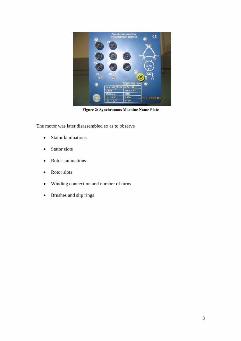
Figure 2: Synchronous Machine Name Plate The motor was later disassembled so as to observe

• Stator laminations

• Stator slots

• Rotor laminations

• Rotor slots

• Winding connection and number of turns

• Brushes and slip rings

3

Figure 3:Stator Upper View

Figure 4: Stator Coils and Laminations

Figure 5: Rotor Side View Figure 6: Rotor Coils and Laminations

Figure 7:Motor Brushes

4

Observations and Dimensions

At this stage, precise measurements of the machine components dimensions were

taken. Later on, these measurements will allow further analysis of the machine.

1. Stator

Observations

Upon observation, the stator consists of 36 slots. It was also estimated that the

number of turns per slot is 60 slots.

Dimensions

The following dimensions were taken;

• Length of the stator : 13.6 cm

• Inner diameter of the stator : 7.0 cm

• Outer diameter of the stator : 11.1 cm

• Width of Stator slots: 0.3 cm each

2. Rotor

Observations

Upon observation, the rotor consists of 18 slots. It was also estimated that the

number of turns per slot is 75 turns.

Dimensions

The following dimensions were taken;

• Length of the rotor : 13.6 cm

• Inner diameter of the rotor (diameter of the back iron) : 2.35 cm

• Outer diameter of the rotor : 6.95 cm

• Width of rotor slots: 0.6 cm each

5

3. Air Gap

The width of the air gap was measured to be 0.5 mm

Experimental Procedure

The main objective was to find the machine's flux φ . This flux will be used to

validate the theoretical and simulated results in future parts of the report. To reach this

goal, an experiment was performed were the machine was running as an open

circuited generator and values of the induced voltage was recorded for different

speeds at constant field current.

The circuit was connected as shown in the figure below and the experiment was

performed according to "Machine's Lab Manual".

Figure 8: Experiment Connections

6

PART ONE

The synchronous generator was mechanically coupled to a prime mover. To change

the speed of the synchronous generator the prime mover speed was altered. This speed

was changed by changing the dc field excitation of the prime mover. The field current

of the synchronous generator is adjusted at its rated value which is equal to 0.95 A.

The no load voltage was measured using a voltmeter and the speed of the rotor was

measured using a stroboscope. The results are summarized in the table below:

Table 1:Data of Experiment 1 Rated Field Current

Synchronous Generator If =0.95A

Ea(V) ω(rpm)

387 1240 390 1250 394 1260 397 1275 401 1285 404 1295 407 1310 411 1320 414 1330 418 1345 422 1360 430 1385 437 1410 443 1430 445 1440 448 1450 451 1460 455 1470 462 1490 466 1510 471 1525 475 1540 481 1560 488 1575 496 1605 501 1625 504 1635

7

The results were plotted on an excel sheet.

No Load Volatge-Speed Graph

y = 0.2957x + 20.357

0

100

200

300

400

500

600

1240

1260

1285

1310

1330

1360

1410

1440

1460

1490

1525

1560

1605

1635

Speed (rpm)

No L

oad

Vol

tage

(V)

Graph 1: Experiment 1 Graph

By linear regression the above graph was approximated into a straight line of equation

0.2957 20.357tV ω= + .

The estimated value of the no load voltage at the rated speed (1500 rpm) is

267.8aE V=

Analysis and Calculations

To calculate the flux of the machine, several steps were considered. Noting that

φωKEa = [5]

where K is a constant representing the construction of the machine

2CN

K = [5]

where is the number of turns per coil of a stator . CN

Knowing that it is a three phase machine therefore the stator has three coils. The stator

also has 36 slots which imply that we have 12 slots per phase. Since each slot contains

8

60 turns as previously mentioned then the total number of turns per coil will be

turnsNC 720=

Therefore: 12.5092

720==K .

Finally to calculate the flux of the machine

3267.8 3.3 102509.12 150060

aE x WbK x x

φ πω−= = =

Theoretical Approach

Synchronous machines are machines whose magnetic field current is supplied

by a separate dc power source. In synchronous motors, torque is produced due to the

presence of two magnetic fields. One magnetic field will be produced in the stator and

the other in the rotor .A torque will be induced in the rotor which will cause it to turn

and align itself with the stator magnetic field. The stator magnetic field rotates. The

induced torque in the rotor will cause it to constantly chase the stator magnetic field.[5]

There are two major concepts of any machine design that should be considered,

magnetic loading and electric loading. Together they will produce the torque of the

machine.

1. Electric loading: is the total current per unit periphery of the stator bore.

2. Magnetic loading is the total number of magnetic lines, cut by each conductor,

in one complete revolution. It is the flux that is coming out of the rotor.

Electric Loading

Electric loading depends on the following factors:

9

1. Allowable temperature rise

2. Heat dissipation capability of the motor enclosure

3. Duty cycle

Starting from the definition of electric loading, it will be formulated as: [4]

a

wp

DAKJK

Qπ

=

Where Da is the rotor diameter

Kp is the packing factor or the ratio of copper area to the total winding area

Kw=fraction of conductors being used to total conductors=1

A is the total winding area

J is the current density

Pwindingstator

slotperturnper

Pslot

slotperturnper

slotperCu

slotperturnper

slotperCu

slotintotal

KA

NIKA

NIA

NIAI

J×

×=

×

×=

×==

36

Therefore,

mKAD

KNIQ

a

wslotperturnper /85.140695.0

136605.136=

×××=

×××=

ππ

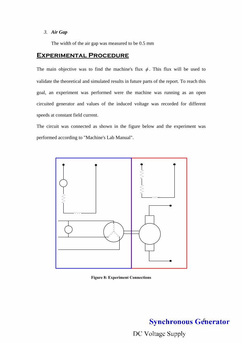
Magnetic Loading

In order to find the magnetic loading, an equivalent circuit of the system is obtained,

shown in the following schematics: [5]

10

The obtained equations are:

11

Figure 9:Pole Model

Figure 10: Magnetic Model

sR

2aR

1aR

rRNi=ℑ

Figure 11: Equivelant Magnetic Circuit

WbturnsKAxxxA

lR

WbturnsKAxxxxA

lR

WbturnsKAxxxxA

lR

mxldAA

mxlddA

mdl

mdl

ao

aa

ror

rr

sor

ss

ar

inouts

r

s

/.59.910148.4104

000005.0

/.67.610148.41042000

0695.0

/.694.22210558.11042000

0872.0

10148.4076.040695.0

4

10558.1076.02

07.0111.02

0695.0

0872.04111.0

4

37

37

37

23

23

===

===

===

====

=−

=−

=

==

===

−−

−−

−−

−

−

πµ

πµµ

πµµ

ππ

ππ

WbturnsKARRRRR aarstotal /.544.24821 =+++=

The number of slots in the rotor is 18 with 75 turns each.

Therefore the number of slots per pole is 4.5 and the number of turns per pole is

poleperturnsturnsx 16975.1682

5.475≈=

In conclusion the magnetic loading of the rotor

Wbxx

xRNi

R totaltotal

43 1045.6

10544.24895.0169 −===

ℑ=φ

MagNet Simulation

12

The synchronous machine is modeled on MagNet Software which is a finite

element analysis software. The finite element analysis will be performed on static 2D.

The choice of 2D will not take into effect the magnetic fields on the boundary of the

machine since it will assume infinite length, but according to literature review this

method will provide accurate results with a tolerance 2%. Thus our choice of 2D

solving is justified.

The machine is represented as a generator by supplying the rotor with

0.95A/turn and supplying no current to the stator. Due to symmetry, one pole of the

generator will be modeled.

The orientation of flux lines are shown in figure1 below.

Figure 12: Synchronous Motor MagNet Simulation

The flux through the center of the above pole is minimal and almost

approaching zero. This is due to the presence of opposing flux fields of equal

magnitudes at the symmetry axis. The opposing field is present due to the right hand

rule, while the equal magnitude is present due to geometrical symmetry and constant

current density through out the copper. Figure 13 will illustrate this phenomenon.

13

Figure 13: Flux Lines Path

On the other hand as we move away from the center, the flux will increase and

it will reach its maximum at the point were the current changes its sense. This is due

to the fact that at this point, all the flux lines have the same sense which is determined

by the right hand rule.

Figure 14: Flux Lines Path The flux obtained upon simulation is:

-33.918 10 Wbφ = × .

A similarity was revealed between the experimental ( ) and the

simulated ( ) values of the flux, which validates the simulation

results.

33.3 10 Wbφ −= ×

-33.918 10 Wbφ = ×

Permanent Magnets & their Applications

14

Permanent Magnet Materials

A permanent magnet, just like any other magnet, will produce a magnetic field

of its own once subjected to a strong external magnetic field. However, the very

special characteristic of the permanent magnet is that it will continue to exhibit a

magnetic field even with the external magnetic field being removed. This produced

magnetic field is said to be continuous if the material doesn't experience a change in

the environment. A change in the environment, for example temperature or

demagnetizing field, will redefine the capabilities of the permanent magnet or

sometimes cancel them. Therefore the more the permanent magnet withstands these

changes the better are its capabilities, and the more successful are its applications. [8]

Brief history of permanent magnets

The historical review of permanent magnet allows a

good vision of the development of such materials with

respect to enhancement in their properties, feasibility of

their applications. Figure 15:Gilbert's Loadstone

The early forms of permanent magnets were described in 1600 by W. Gilbert. They

are called “loadstone with soft iron pole tips” .These are a form of magnetite Fe3O4

that had iron tips that increase attractive forces upon contact .They are used to

magnetize pieces of iron and steel.

In 1825, J. Henry and W. Sturgeon invented the electromagnet.

15

Figure 16: Henry Electromagnet

By the year 1867, German scientists started making ferromagnetic elements from

nonferromagnetic material and nonferromagnetic alloys from ferromagnetic materials

like iron.

In 1901 Heusler alloys were discovered. Heusler alloys contain 10 to 30 percent

manganese and 15 to 19 percent aluminum and copper.

In 1917 cobalt steel alloys were discovered.

In 1931 alnico (Al, Ni ,Co ,Fe ) were discovered.

In 1938 powdered oxides were developed.

Figure 17:Alnico

In the 1950 ferrites (barium ferrite BaOx6Fe2O3 and strontium ferrite SrOx6Fe2O3)

were invented. Hard ferrite (ceramic) magnets were developed in the 1960's as a low

cost alternative to metallic magnets is SrO-6(Fe2O3), strontium hexaferrite.

Figure 18: Ferrite Permanent Magnet

16

In the 1970’s rare earth permanent magnets (samarium-cobalt SmCo and neodymium-

iron-boron NdFeB) were developed.

Figure 19: Neodymium-iron-boron

Figure 20: Samarium Cobalt

Since then Rare earth permanent magnets are being increasingly used in machine

industry.

In 2002, NdFeB became the most abundant of all permanent magnets. [8]

General Properties of Permanent Magnet Materials

In designing for a permanent magnet application, several characteristics of that

material are considered. The most important characteristic is the demagnetization

curve which will allow the designer to judge whether the permanent magnet used is

suitable for the application being designed. Also the material properties, the shape of

the magnet and the operating conditions are essential factors that might constrain or

simplify the achievement of a successful design. [8]

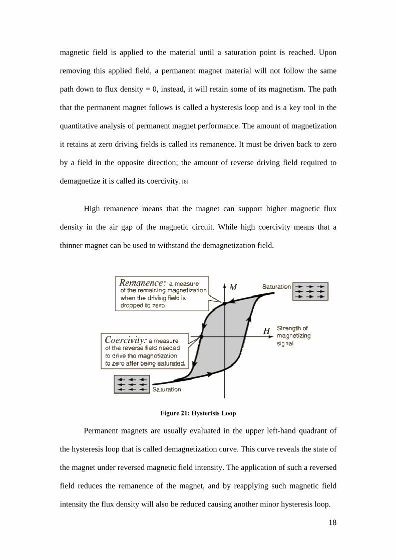
Hysteresis Loop

A permanent magnet does not need any excitation winding to produce

magnetic field in an air gap nor does it lead to dissipation of electric power.

Permanent magnets can be described by the B-H hysteresis loop. They are usually

considered to have wide hysteresis loops. During magnetization, an increasing

17

magnetic field is applied to the material until a saturation point is reached. Upon

removing this applied field, a permanent magnet material will not follow the same

path down to flux density = 0, instead, it will retain some of its magnetism. The path

that the permanent magnet follows is called a hysteresis loop and is a key tool in the

quantitative analysis of permanent magnet performance. The amount of magnetization

it retains at zero driving fields is called its remanence. It must be driven back to zero

by a field in the opposite direction; the amount of reverse driving field required to

demagnetize it is called its coercivity. [8]

High remanence means that the magnet can support higher magnetic flux

density in the air gap of the magnetic circuit. While high coercivity means that a

thinner magnet can be used to withstand the demagnetization field.

Figure 21: Hysterisis Loop

Permanent magnets are usually evaluated in the upper left-hand quadrant of

the hysteresis loop that is called demagnetization curve. This curve reveals the state of

the magnet under reversed magnetic field intensity. The application of such a reversed

field reduces the remanence of the magnet, and by reapplying such magnetic field

intensity the flux density will also be reduced causing another minor hysteresis loop.

18

New Permanent Magnet Materials

The permanent magnets that are currently used for electric motors are:

1. Alnicos (Al, Ni, Co ,Fe )

2. Ferrites (barium ferrite BaOx6Fe2O3 and strontium ferrite SrOx6Fe2O3)

3. Hard ferrite SrO-6(Fe2O3), strontium hexaferrite

4. Rare earth permanent magnets (samarium-cobalt SmCo and neodymium-iron-

boron NdFeB)

Alnico

It has a high magnetic remanent flux density. This advantage will allow a high air gap

magnetic flux density. However, the coercivity is very low and the demagnetization

curve is considered to be non-linear so although it is easy to magnetize alnico, it is

also easy to demagnetize it .They are used in dc commutator motors and in motors

with few Watts up to 150KW, however ferrites became more popular. [8]

The key attributes of Alnico are:

• Mechanically strong

• Cast to a variety of shapes

• Very temperature stable

• Can change magnetic orientation

• High Bmax characteristics compared to ceramic materials.

19

Ferrites

A ferrite has a higher coercive force than alnico. Lower remanent magnetic

flux density, low cost and very high electric resistances are its main advantages since

no eddy current losses in the PM volume will occur. Moreover they have an economic

advantage over Alnico. They are commonly used in small DC commutator motors.

The key attributes of Ferrites are

• Economical

• Good for simple shapes only

• Very fragile

• Require expensive tooling

• Temperature sensitive (0.2%°C).

Hard Ferrites

Hard Ferrite has normal operating capabilities between -40°C and +250°C. As

temperature increases, remanence decreases whereas coercivity increases. At very low

temperatures there is a risk of permanent demagnetization in magnet systems.

When it appeared that no further significant improvements would be made to ferrite

magnets the search began in 1960’s for other materials with high saturation

magnetization. [1]

Rare Earth Permanent Magnets

It is the newest type of permanent magnets that has been widely used in the

last two decades. It is mostly used in electrical machines. The elements of this type of

magnets are natural minerals that are widely available and used as mixed compounds.

High performance of rare earth magnets has successfully replaced Alnico and ferrite

20

magnets in all applications where the higher efficiency is required. Samarium cobalt

SmCo5 has the advantage of high remanent flux density, high coercive force, linear

demagnetization curve and low temperature coefficients. It is well suited to build

motors with low volume and high power density. It faces a major draw back which is

its high cost due to the lack of Sm and Co.

In 1983, researchers discovered the inexpensive neodymium Nd which

lowered the raw material cost. NdFeB magnets have better magnetic properties than

SmCo5 but only at room temperature. Their disadvantage lie in the fact that their

demagnetization curves mainly the coercive force is strongly temperature dependant.

However this magnet faces corrosion. In year 2002, these magnets showed higher

remanent magnetic flux density and better thermal stability.

The permanent magnet motor was conceived by Howard Robert Johnson

sometime after the 1940s. Allegedly it is a design for a perpetual motion machines.

Reportedly, the device is designed on the principle that a constant imbalance of the

magnetic forces between the rotor and the stator is created. [8]

The key attributes of Samarium cobalt are

• Quite expensive

• High Bmax

• Very good temperature stability

• Powerful for size

The key attributes of Neodymium Iron Boron are

• High energy for size

• More economical than Samarium Cobalt

• Good in ambient temperature situations

21

• Relatively high price

• Corrosion that can result in loss of energy

• Temperature coefficient of 13% degree centigrade.

Application of Permanent Magnets in Motors

The most important application of permanent magnets is in electric motors.

With the development of these materials and the introduction of the rare earth

magnets, more focus was directed towards the electronic devices, since these magnets

provided a shift towards the electronic evolution of electric motors.

Permanent magnets are widely used in DC Motors. Recent DC motors widely

employ Rare Earth Magnets. Another category of motors where permanent magnets

are used is Stepper Motors .Less widely used, but still effectively employed, are the

Synchronous Motors with permanent magnets.

We note here that since our model is a conventional synchronous motor, our

concern will later be to realize the effectiveness of using a permanent magnet in the

existing motor. [8]

Benefits of using permanent magnets in electrical machines [8]

• The field excitation circuit in the case of electromagnetic excitations will

exhibit excitation losses due to the energy absorbed by that circuit. However in

the permanent magnet machines no such excitation exists therefore we have an

increase in efficiency

• Consequently a higher torque or output power is established in the system

• With the presence of a permanent magnet a higher magnetic flux density will

be established in the air gap

• Lower complexity in construction

22

• Permanent magnets implies that the machine is brushless therefore

maintenance is simplified

• Lower prices for certain types of machines.

Application of Permanent Magnets in DC-Motors

Permanent magnets are widely used in DC motors. In conventional DC

motors, the armature windings provide the technique for controlling the speed of the

motor; also the field winding provides the excitation of the motor. However with the

introduction of permanent magnets into the DC machine, we started having more

efficiency and less complexity in the provision of magnetic field.

Lately, the range of application of these motors broadened especially with the

use of the high energy rare earth magnets, since they are able to produce larger

magnetic fields with a much smaller and much lighter magnet. With these permanent

magnets being used, brushes and commutator segments became unnecessary. The PM

DC motor is also referred to as Brushless DC motor. One of the basic advantages of

having a permanent magnet, especially rare earth magnets, in the DC machine is that

it will eliminate the mechanical switching of the armature current. This switching will

be performed electronically in the presence of the magnet. Also, by using rare earth

magnets, the rotor of the machine will be built with lower inertia; also these magnets

allow a higher air gap flux which means a higher output torque. With the high

coercivity the rare magnet have, an improvement of resistance to demagnetization

from motor's own armature winding is obtained.

DC brushless motors are widely used in automobiles, blowers, starters,

radiator cooling fans, and computer hard disk drives. [8]

23

Application of Permanent Magnets in Stepper-Motors

A stepper motor is known to rotate in a sequence of discrete steps. With this

manner of operation, they are usually digitally controlled. They are commonly used in

application of incremental motion for example printers, plotters, and computer

peripherals.

The mode of operation of a stepper motor requires a variable reluctance to be

established between the stator and the rotor. Also we need an air gap flux to be

produced. In conventional stepper motors, this flux is solely produced by the armature

winding. The use of a permanent magnet will help in the production of this flux and

will therefore increase the air gap flux. With this increase in flux, the torque will

increase, and efficiency is improved.

In hybrid stepper motors, the permanent magnet is built into the rotor. Soft

iron rotor cups will sandwich this magnet. The permanent magnet will help in the

creation a strong holding torque, which is one of the major characteristics of the

stepper motor. The armature winding usually switches the magnetic field to different

angular positions in the air gap; the use of permanent magnet is to maximize the

difference in magnetic fields in the air gap so as to maximize the holding torque.

Alnicos are widely used in hybrid stepper motor. Some designs use rare earth magnets

since they provide lower inertia. [8]

Another type of stepper motors that uses the permanent magnet is called the

can-stack motor. The difference between the hybrid and the can-stack motor is that

the latter has no iron rotor cups, and the permanent magnet is cylindrical with a shaft

passing through it. Ceramic ferrites are commonly used in this motor. Also rare earth

magnets are being used recently. These motors are used in applications large volumes.

24

Application of Permanent Magnets in Synchronous-Motors

With the introduction of permanent magnets to synchronous motors,

commutation was cancelled. The permanent magnet in a synchronous motor will

rotate in synchronous with the armature field. It will produce a maximum torque when

the magnetic field from the permanent magnet and that of the armature are at 90º

difference.

Synchronous motors with permanent magnets are good in applications of

constant supply voltage and constant frequency; they are also good for applications of

variable frequencies. These motors have a better efficiency, higher power factor, and

higher power density. However these machines have a weak starting torque.

Permanent magnet synchronous motors performs like the conventional motors

once the flux from the magnet takes over and allows the synchronization of rotor and

stator. We must note that the initial field excitation is performed by the permanent

magnet itself.

Usually, high coercivity permanent magnets are used in synchronous

machines, because the synchronization speed will force the magnet material to

experience a strong demagnetization field. Ceramic ferrite and rare earth magnets are

mostly employed in synchronous motors. [8]

These motors are commonly used with ratings of 15 KW .They are also

available with ratings up to 746 KW. Recent developments can reach 1MW using rare

earth permanent magnets. [8]

PM synchronous motors have five classical rotor construction configurations: [

1. Merrill's Rotor:

It was the first successful construction of PM synchronous

motor. It is characterized by small power ratings and high frequency.

25

Alnico permanent magnet is used for this configuration. Alnico is

placed on the shaft with the help of aluminum sleeve. It is important to

note that the PM will not be demagnetized since the applied reverse

flux at starting or reversal will only pass through the laminations and

slots and not through the PM.

2. Interior Type PM motor:

This type of motor used for high frequency and high speed. It

has a high protection against demagnetization because the flux line can

pass through the rotor without passing through the PM.

3. Surface PM motors:

This type of motor will have its magnet magnetized radially.

Sometimes an external non ferromagnetic cylinder is used for the

magnetization process. It has a simple construction; however it has a

lower air gap magnetic flux than other types of PM synchronous

motors. Also one of it main disadvantages is that the permanent

magnet of the surface PM motors is not protected against

demagnetization.

4. Inset Type PM motors:

This type has it magnet embedded in shallow slots of the rotor.

Also, its magnet is magnetized radially. Just like the surface PM

motors, this motor requires a non ferromagnetic cylinder. The emf

induced by these motors is lower than that of the surface motor.

26

5. Buried PM motors

These have circumferentially magnetized permanent magnets

that are embedded in deep slots. It needs a non ferromagnetic shaft

since using ferromagnetic shafts will cause a large portion of useless

magnetic flux to go through the shaft. These motors have the largest air

gap magnetic flux density among all the other types. The permanent

magnet in the rotor is protected against armature fields i.e.

demagnetization. However it is relatively complicated in construction.

27

Permanent Magnet Design

Magnet Choice

In permanent magnet synchronous machines the choice of magnet type is of

vital importance. Usually, high coercivity permanent magnets are used, since the

synchronization speed will force the magnetic material to experience a strong

demagnetization field. Ceramic ferrite and neodymium iron boron are mostly

employed in such machines.

Table 2: Magnet Properties [1] Br (T)

(Magnetic Remanence)

HC (KA/m)

Coercivity µr

Ceramic Ferrites 0.4 265 1.15 Sintered NdFeB 1.1 700 1.05

As shown in table 2, the magnetic remanence and the coercivity of ceramic

ferrites is lower than that of sintered NdFeB. High remanence means that the magnet

can support higher magnetic flux density in the air gap of the magnetic circuit. While

high coercivity means that a thinner magnet can be used to withstand the

demagnetization field. In this project, the optimization procedure will be implemented

on both types and a later comparison between the two will show the effect of the

magnet type on the overall machine.

Rotor Configuration

As shown in the previous sections, PM synchronous motors have five classical

rotor construction configurations, the Merrill's Rotor, the Interior Type rotor, the

Surface Type rotor, the Inset Type rotor and the Buried type rotor. For the purpose of

this project, the surface type configuration will be selected. This configuration doesn’t

concentrate the flux in a process known as flux focusing as other configurations do.

28

This is vital for this project since flux focusing is normally us with magnets of low

remanence, in order to increase the flux in the air gap. But this will cause undesirable

saturation if it is used with magnets of high remanence such as NdFeB. In addition,

this configuration will have its magnet magnetized radially. Moreover, the equations

that govern the surface type configuration are simpler than other configurations. Thus

the design theory will be simplified. The configuration of the rotor is cylindrical with

no opening in the middle as in the other configurations; this will simplify the

manufacturing and assembly procedure. For this reason, cost will be reduced.

Figure 22: Surface Type Mounted Configuration

The w

magnet rotor

permanent m

will improve

split ratio ana

produce an im

ound rotor of the synchronous machine is replaced by a permanent

using Ceramic Ferrites and NdFeB magnets. The introduction of a

agnet into the machine will increase the magnetic remanence and hence

the magnetic loading which will increase the output torque. Furthermore,

lysis is applied so as to obtain the optimal machine parameters that will

proved electric loading and thus further augment the output torque.

29

Figure 23 illustrates the rotor configuration along with the machine parameters:

Figure 23:Rotor Configuration Machine Parameters La : the length of the machine As : slot area Sd : slot depth tP : tooth pitch Wt: tooth width dbi : back iron depth Ns : total number of slots Lm : magnet thickness Lg : air gap Dr : rotor diameter Do : stator diameter Kp : packing factor Q : electric loading Bg : air gap magnetic flux density ab : slot outer width cd : slot inter width D1 : distance from center to the beginning of the slot D2 : distance from center to the ending of the slot Kp : slot packing factor Pc : copper losses

30

Split Ratio Analysis

The split ratio analysis [1][2][3] is a technique that optimizes the output torque of

the machine by finding the corresponding rotor to stator diameter. This is performed

by formulating the output torque as a function of the machine parameters, then

differentiating it with respect to the split ratio and setting its value to zero.

Torque Equation Derivation

The force (F) acting on a current-carrying conductor in a magnetic field (B) is

where I is the current passing through one conductor and L. . aF B I L= a is the active

axial length.

Figure 24: Machine Representation

The torque per conductor is . . . .2 2

r ra

D DT F B I L= =

Therefore, the torque for N conductors is:

. . . .2 2

r rav a

D DT F B I L N= = .

31

Due to the fact that the value of the current I varies from one design to another, the

electric loading will be considered as a more suitable parameter to account for Dr and

N.

The electric loading:

. ( /.

. .

rms

r

rrms

N IQ ampsD

Q DIN

ππ

=

⇒ =

)m

Substituting Irms in the torque expression gives:

2 2

22

2

2

av a

av a

Q D DT B L NN

T Q D B L

π

π

× ×= × × × ×

∴ = × × × ×

Split Ratio Equation

The Torque of any machine is defined by the output power divided by the

angular speed. PT P Tωω

= ⇒ = .

2

2 r a gP D L B Qπ ω∴ = where Bg is the magnetic flux density in the air gap which is

approximated to be equal to Bav

The power to volume ratio:

2

0

2 arg

o

LDP B QV D L

ω⎛ ⎞

= ⎜ ⎟⎝ ⎠

Thus, the Torque to volume ratio: 2

0

2 arg

o

LDT B QV D L

⎛ ⎞= ⎜ ⎟

⎝ ⎠

Let ξ be the split ratio

r

o

DD

ξ =

32

Thus, 22 ag

o

LT B QV L

ξ=

In order to optimize the torque, both the electric loading Q and magnetic loading Bg

should be formulated for this specific machine.

Magnetic Loading

It is defined as the magnetic flux density in the air gap1

rg

gr

m

BB ll

µ=

+

Electric Loading

The electric loading is defined by s p s

r

JA K NQ

Dπ=

Where c

s a

PJ

A Lρ=

Thus p s c s

r a

K N P AQD Lπ ρ

=

Using the geometry of the surface type chosen configuration, which is shown in

figure23.

2 20 21 ( )

4 4bi r

s t o bi rs

D d DA W D d D

Nπ π⎡ ⎤−⎛ ⎞= − − −⎢ ⎥⎜ ⎟

⎝ ⎠⎢ ⎥⎣ ⎦−

Non-Saturation Criteria

In addition, the machine should avoid saturation, thus the magnetic field

density in the iron should not exceed Bmax=1.1T. Applying the Continuity Theorem of

the flux, the flux in one slot of the air gap is equal to the flux corresponding to one

slot in the iron of the stator.

33

/ max

max

airgap tooth

g airgap tooth tooth

g p a t a

B A B A

B t L B W L

φ φ=

× = ×

× × = × ×

max

g pt

B tW

B×

= (First Saturation Criteria)

The flux is divided along the magnet in two

directions to two parts each of a value max

2φ .

p

WBN

dB

pN

ts

bi

slotpersironback

ironbackslots

2max

max

××=×

×=

=

φφ

φφ

2s t

biN Wd

p×

= (Second Saturation Criteria)

Geometry Parameters

Other machine parameters are obtained directly from the geometry of the machine.

rp

s

Dt

Nπ ×

=

1

2

1

2

1 2

22

2

o bi

r g

ts

ts

d

D D dD D l

Dab WN

Dcd WN

D Ds

π

π

= −

= +

×= −

×= −

−=

34

AS Formulation

Using the saturation criteria and substituting them in As, we get:

( ) ( )2 221 . .4 4 2

rrs s t

s

OD dbi OD dbi DDA N WN

π⎡ ⎤⎡ ⎤− − −⎢ ⎥= − −⎢ ⎥⎢ ⎥⎢ ⎥⎣ ⎦⎣ ⎦

( )2 22

2 2

2. .

4 2 2pr r

2r

s s ts m

BOD dbi D D DOD ODA NN OD OD B p

π π⎡ ⎤W

⎡ ⎤− ⎛ ⎞= − − − −⎢ ⎥ ⎢ ⎥⎜ ⎟

⎢ ⎥ ⎝ ⎠⎣ ⎦⎣ ⎦

2 2 22 2

2 2 2 2

41 44 2 4

12 2 2

p pr rs

s m m

p p p pr rr r

s m m m m

B BD DODAN OD B p B p OD OD

B B B BD DOD D DN B B p B B

π π π

ππ π

⎡ ⎤= − + −⎢ ⎥

⎢ ⎥⎣ ⎦⎡ ⎤

− − −⎢ ⎥⎣ ⎦

r

r

D

Dπ

2 222 2

2 2 2 2

22 22 14

p p p p pr rs

s m m m m m

B B B B BD DODAN OD p B p B B OD p B B

π π π π⎡ ⎤⎛ ⎞ ⎛ ⎞= + + − − +⎢ ⎥⎜ ⎟ ⎜ ⎟⎜ ⎟⎢ ⎥⎝ ⎠⎝ ⎠⎣ ⎦

1+

22

4ss

ODAN

π αξ βξ λ⎡ ⎤= −⎣ ⎦+

Where

2

max max

2 2 2g gB BB p p B

π πα⎡ ⎤⎛ ⎞ ⎛ ⎞⎢ ⎥= + + +⎜ ⎟ ⎜ ⎟⎢ ⎥⎝ ⎠⎝ ⎠⎣ ⎦

1−

max

3 1gBB p

πβ⎛ ⎞

= +⎜ ⎟⎝ ⎠

1λ =

35

Torque Formulation

Substituting the above equations in the Torque equation will lead:

2.T y ξ αξ βξ λ= + +

2.5

2(1 )gr

m

er o a p

ll

yhB D l k

µ

ρ

+= which is a constant

Torque Optimization

Optimizing the torque by differentiating the right side of the equation with respect to

the split ratio:

2 322

dTd

αξ βξξ= + + λ

Setting the above equation to zero, the split ratio corresponding to the optimal Torque

is determined by:

( )21.5 1.5 84

β β αξ

α− ± −

=λ

36

Code Formulation

To apply the above optimization procedure, a certain algorithm was followed so as to

obtain the optimal machine parameters and output values. The logic behind the

algorithm is shown in the flowchart of figure. The code for this flowchart is simulated

on MatLab (refer to appendix).

Optimization Results

The optimization results of the MatLab code are applied to permanent magnet

designs. The first design used a Ceramic Ferrite magnet while the second design used

a sintered NdFeB magnet. The results are listed in Table 3.

37

Table 3: Optimized Machine Parameters

Machine Parameters Ceramic Ferrites Sintered NdFeB TP 5.7 4.1

Wt 1.3 2.5 dbi 5.8 11.4

D1 99.4 88.3 D2 65.7 46.5

ab 7.4 5.2 cd 4.4 1.5

Sd 16.9 20.9 La 136 136

Lm 5 5 Lg 0.5 0.5

Dr 64.7 45 Do 111 111

Making use of the preceding values, the calculated torque for both magnet designs is

, T N 5.5 .FerritesT N m= 9.1 .NdFeB m=

= 20.5 /NdFeBQ kA m=

And the obtained electric loading is:

17.25 /FerritesQ kA m ,

38

Magnet simulation

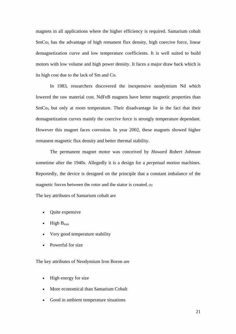
To test the obtained results, the optimized machine was modeled and

simulated using MagNet software. The flux and induced voltage were then computed.

The initial flux field diagrams are shown below:

Figure 25: Optimized Design Flux Lines using Ceramic Ferrites

Figure 26:Optimized Design Flux Lines using Sintered NdFeB

39

The maximum flux obtained in the air gap for both designs is found to be:

37.15 10Ferrites Wbφ −= × and 316.33 10NdFeB Wbφ −= ×

No load Voltage Calculation

To calculate the induced no load voltage Ea, the rotor was rotated in steps of 3 º

mechanical. This was performed by the following steps:

1. Sectionalizing the magnet of one pole of the machine into 30 segments

2. Assigning different polarities to each fragment of the pole and rotating the

pole in steps of three degrees.

The flux is recorded for each rotation at a particular point inside the air gap and its

variation for one cycle is graphed.

-0.008

-0.006

-0.004

-0.002

0

0.002

0.004

0.006

0.008

0 60 120 180 240 300 360

Electrical Degree

Air

Gap

Flu

x (W

b)

Graph 2: Flux Variation for Ceramic Ferrites

40

-0.02

-0.015

-0.01

-0.005

0

0.005

0.01

0.015

0.02

0 60 120 180 240 300 360

Electrical Degree

Air

Gap

Flu

x (W

b)

Graph 3: Flux Variation for Sintered NdFeB

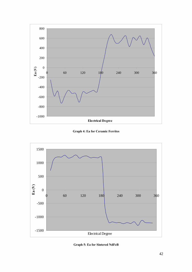
Then, the difference between two consecutive flux values was calculated so as to

obtain the value of dφ . The value of dt was computed using the following relation:

3 60sec 0.33 sec360 1500

dt mrpm

⎛ ⎞°= × =⎜ ⎟°×⎝ ⎠

Knowing that adE Ndtφ

= and N per pole per phase is 180, the induced voltage is

obtained. The following plot illustrates the induced no load voltage for one electric

cycle for the two designs.

41

-1000

-800

-600

-400

-200

0

200

400

600

800

0 60 120 180 240 300 360

Electrical Degree

Ea

(V)

Graph 4: Ea for Ceramic Ferrites

-1500

-1000

-500

0

500

1000

1500

0 60 120 180 240 300 360

Electrical Degree

Ea

(V)

Graph 5: Ea for Sintered NdFeB

42

Comparative Analysis

The torque of the machine has increased up to 3 times using Ceramic Ferrite

magnets and 5 times using the Sintered NdFeB magnet while keeping the speed of the

machine constant and maintaining the machine size.

The output torque depends on the magnetic and electric loading of the machine.

This increase in the torque value for both designs is justified by the following reasons:

1. The permanent magnet that replaced the wound rotor coils has a magnetic

remanence of 0.4T for Ceramic Ferrites and 1.1T for Sintered NdFeB rather

than 0.3T of the conventional machine.

2. The stator slots became wider and thinner than that of the conventional

machine for both designs thus allowing more copper concentration per slot

which implies a greater current value and hence an improved value of the

electric loading.

3. Finally, the split ratio technique optimized the dimensions and parameters of

the machine in such a way so that the ratio of the rotor to the stator diameter is

maintained at optimal torque.

43

Table 4: Dimensions Comparison

Machine Parameters Conventional(mm)

Ceramic Ferrites(mm)

Sintered NdFeB (mm)

Tooth pitch 7.8 5.7 4.1 Tooth Width 2.9 1.3 2.5 Back iron depth 8.4 5.8 11.4

Distance from center to the beginning of the slot 36 99.4 88.3

Distance from center to the ending of the slot 47.1 65.7 46.5

Slot outer width (Stator) 4.08 7.4 5.2 Slot inner width (Stator) 3.01 4.4 1.5 Slot depth 12.1 16.9 20.9 Length of the machine 136 136 136 Magnet thickness - 5 5 Air gap length 0.5 0.5 0.5 Rotor diameter 69.5 64.7 45 Stator diameter 111 111 111

Table 5: Parameters Comparison

ConventionalCeramic Ferrites

Sintered NdFeB

Output Torque(N.m) 1.9 5.5 9.1

No Load Voltage(V) 267 353.6 909.7

Flux(mWb) 3.9 7.15 16.33

Electric Loading(kA/m) 14.85 17.25 20.5

44

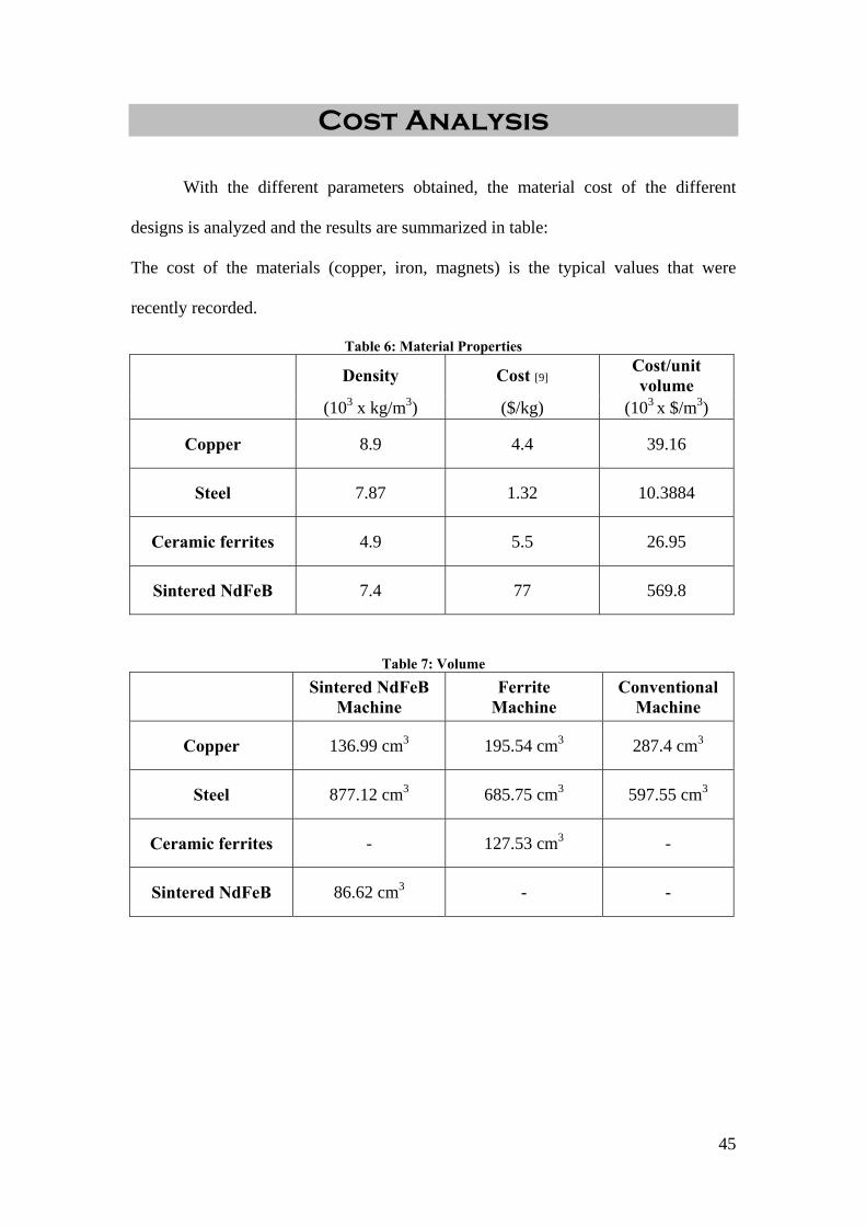
Cost Analysis

With the different parameters obtained, the material cost of the different

designs is analyzed and the results are summarized in table:

The cost of the materials (copper, iron, magnets) is the typical values that were

recently recorded.

Table 6: Material Properties

Density Cost [9] Cost/unit volume

(103 x kg/m3) ($/kg) (103 x $/m3)

Copper 8.9 4.4 39.16

Steel 7.87 1.32 10.3884

Ceramic ferrites 4.9 5.5 26.95

Sintered NdFeB 7.4 77 569.8

Table 7: Volume

Sintered NdFeB Machine

Ferrite Machine

Conventional Machine

Copper 136.99 cm3 195.54 cm3 287.4 cm3

Steel 877.12 cm3 685.75 cm3 597.55 cm3

Ceramic ferrites - 127.53 cm3 -

Sintered NdFeB 86.62 cm3 - -

45

Table 8: Cost

Sintered NdFeB Machine

Ferrite Machine

Conventional Machine

Copper $5 $8 $11

Steel $9 $7 $6

Ceramic ferrites $0 $3 $0

Sintered NdFeB $49 $0 $0

Table 9: Analysis

Sintered NdFeB Machine

Ferrite Machine

Conventional Machine

Total Cost $64 $18 $17

Output Torque 9.10 Nm 5.50 Nm 1.90 Nm

Output Voltage 909.7 V 353.6 V 267 V

The material cost of each of the three designs is estimated above. The conventional

machine has a lower cost than the other two designs; however this design is restricted

in application since it has a lower torque and lower output voltage than any other

design. Knowing that the size of the machine is maintained constant, the higher output

torque and voltage of the optimized designs will have wider applications and efficient

space utilization. Moreover, the higher cost of the permanent magnet machine that

uses the sintered NdFeB is justified by the increase in the torque by five times.

46

Conclusion

With the availability of computer aided programs, optimization of electric

machines is simplified. Upon using MagNet, the analysis of a conventional

synchronous machine came up with satisfactory conclusions. Moreover experiments

performed in the lab, provided an insight in the study and investigation of the machine

magnetic flux and electrical parameters. The optimization that followed the

conventional machine analysis was performed using split ratio technique. With the

flux in the air gap being improved, the torque of the machine was augmented

significantly, making the machine more efficient in power generation. Moreover, the

optimized machine became a potential candidate for applications requiring high

output power in limited space allocation.

47

References

1. Birch T.S., Chaaban F. B., Howe D., Mellor P.H.,(1991) Topologies for a

Permanent Magnet Generator/Speed Sensor for the ABS on Railway Freight

Vehicles, EMD Conference, London. pp.31-35

2. Campbell, P. (1996) .Permanent Magnet Materials and their Application

3. Chaaban, F.B. (1989) Computer Aided Analysis, Modeling and Experimental

Assessment of Permanent Magnet Machines with Rare Earth Magnets, Ph.D.

Thesis, Liverpool University

4. Chaaban, F.B. (1993) Determination of the optimum Rotor/Stator diameter

ratio of Permanent Magnet Machines, IEEE Trans., pp.521-530.

5. Chapman, J. (2005). Electric Machinery Fundamentals

6. Coren, R. (1989)., Basic Engineering Electromagnetics

7. Elsevier Science Publishing. (1989). Computer-aided analysis and design of

electromagnetic devices

8. Gieras, F., Wing, M. (2002). Permanent Magnet Motor Technology

9. Ronghai Q., Thomas A. (2003) Dual-Rotor, Radial-Flux, Toroidally Wound

Permanent Magnet Machines, IEEE Transactions, Vol.39, No. 6

48

ACKNOWLEDGEMENT

The support of Professor F. Chaaban, American University of Beirut, who

assisted the authors in this report, is gratefully acknowledged.

49

Appendix A - Matlab Code clc; clear all; %Magnet Parameters ur=1.15; Br=0.4; %Motor Parameters p=4; Do=0.111; Ns=36; kp=0.4; rho=1.72e-8; Pc=20;%The total losses of a machine are taken to be 10% %of the total output power of the machine which is 300W %Therefore, the total power losses=30 W %So, the copper losses as 20W since the core losses amd other

% losses constitute a low percentatge of the total losses %at rated values.

La= 0.136 ;Bmax=1.6; %Material Costs CCU=53.4e3;%Copper CST=7.87e3;%Iron Cmag=1110e3;%Magnet % Inital Conditions lm=0.005;% Magnet Length lg=0.0005;% Air Gap Length %Calculating Optimum Bg=Br/(1+ur*lg/lm); a=(Bg/Bmax)^2*((pi/p)^2+2*pi/p)+2*Bg/Bmax-1; b=-Bg/Bmax*(2*pi/p+2); c=1; a1=2*a; b1=3/2*b; ratio=(-b1-(b1^2-4*a1*c)^0.5)/(2*a1); Dr=ratio*Do; tp=pi*(Dr+2*lg)/Ns; Wt=Bg*tp/Bmax; db=Wt*Ns/(2*p); d1=Do-2*db; d2=Dr+2*lg; ab=pi*d1/Ns-Wt; cd=pi*d2/Ns-Wt; Sd=(d1-d2)/2; As=Sd*(ab+cd)/2; Acu=As*kp*Ns; T=((La*Bg^2*Dr^2*Pc*Acu)/(4*rho))^0.5;

50

J=(Pc/(Acu*La*rho))^0.5; Q=J*Acu/(pi*Dr); SSA=pi/4*(Do+d2)*(Do-d2)-As*Ns; RSA=pi/4*(Dr-2*lm)^2; SA=SSA+RSA; Vm=pi*lm*La*(Dr-lm); VCC=La*Acu; VS=SA*La;

51