Faculty of Biosciences, Fisheries and Economics (BFE ...
57
Faculty of Biosciences, Fisheries and Economics (BFE) Department of Arctic and Marine Biology (AMB) Ungulate population monitoring in a tundra landscape: evaluating total counts and distance sampling accuracy — Mathilde Le Moullec Master thesis in Biology, BIO-3950 - May 2014
Transcript of Faculty of Biosciences, Fisheries and Economics (BFE ...

Faculty of Biosciences, Fisheries and Economics (BFE)
Department of Arctic and Marine Biology (AMB)
Ungulate population monitoring in a tundra landscape: evaluating total counts and distance sampling accuracy
— Mathilde Le Moullec Master thesis in Biology, BIO-3950 - May 2014

I
Front page and acknowledgement pictures: Mathilde Le Moullec

II
Ungulate population monitoring in a tundra landscape:
evaluating total counts and distance sampling accuracy
Mathilde Le Moullec
BIO-3950
Master’s thesis in Biology
Northern Population and Ecosystems
May 2014
Supervisors
Nigel Gilles Yoccoz, The Arctic University of Norway (UiT)
Åshild Ønvik Pedersen, Norwegian Polar Institute (NPI)
Brage Bremset Hansen, Norwegian University of Science and Technology (NTNU)

III
IV
Abstract
Researchers and managers are constantly working towards decreasing monitoring
uncertainties in order to improve inferences in population ecology. The solitary and sedentary
Svalbard reindeer (Rangifer tarandus platyrhynchus) inhabit a high-Arctic tundra landscape
highly suitable to compare accuracy (precision and bias) of population monitoring methods in
the wild. The flexible Bayesian state-space model enabled me to assess uncertainties in
estimates of the abundance of four reindeer sub-population time-series. In this environment,
Total population Counts (TC) were more precise than Distance Sampling (DS), especially
when conducted multiple times during a field season (e.g. Sarsøyra, summer 2013: DS
Coefficient of Variation (CV)= 0.11, only one TC CV= 0.06; four repeated TC CV= 0.03). In
addition, TC’s bias was assumed low once integrated in the state-space model and related to
re-sightings of marked animals. Conducting DS alone, without TC as background
information, would have estimated wrong reindeer population size because the detection
function was sensitive to sample size. However, the similarity in landscape and methodology
across the two neighboring DS study sites enabled their observations (n= 143) to be pooled,
resulting in more plausible estimates, yet slightly higher than those found through TC. DS is
used worldwide and this study illustrates fundamental issues around the minimum sample
sizes recommended in literature (n>80) and that the number or length of transects must be
sufficient to represent habitat structure (in this particular case the proportion of vegetation).
Furthermore, combining multiple sources of available data in a common modeling
framework, even with wide standard deviation such as DS, resulted in more precise estimates.
Keywords: Line transects, detection probability, Poisson-Poisson sampling, population size,
state-space model, Rangifer.

V
Résumé
Aussi bien les scientifiques que les gestionnaires cherchent à améliorer les incertitudes
inhérentes aux recensements des populations pour ainsi améliorer les inférences en écologie
des populations. Le renne du Svalbard (Rangifer tarandus platyrhynchus) occupe un habitat
aux affinités particulières (i.e. grandes plaines, végétation rase) pour pouvoir comparer
l’acuité (précision et biais) des méthodes de recensements des populations sauvages. Le
« state-space » modèle Bayesien est flexible et a permis de mesurer les incertitudes de
comptages de quatre sub-populations de rennes. Il a également permis de montrer que, dans
cet environnement, la méthode de recensement total de la population (TC) est plus précise que
celle du Distance Sampling (DS) (e.g. Sarsøyra, été 2013: DS CV= 0.11, un seul TC CV=
0.06; quatre TC répétitions CV2013= 0.03). En plus d’être précis, les TC sont supposés être
faiblement biaisés d’après cette étude. Ils m’ont permis de mettre en avant le fait que
sélectionner le meilleur model du DS en suivant les étapes de sélection, aurait, sans regard
critique, donné des estimations erronées. La probabilité de détection du DS s’est monté
particulièrement sensible à la taille de l’échantillon. La similarité des paysages et de la
méthodologie utilisée dans ces deux sites voisins ont permis de regrouper les observations
rendant les estimations plus vraisemblables, même si toutefois, elles restent supérieures aux
TC. Le DS est intensément utilisé à l’échelle mondiale et cette étude illustre l’importance
fondamentale d’avoir un échantillon de taille minimale (n>80) ainsi que de s’assurer d’avoir
suffisamment de transectes pour représenter la structure de l’ensemble de l’habitat étudié
(dans ce cas particulier : la proportion de végétation). Rassembler des données de multiples
sources dans un model commun, même ayant de large intervalles de confiance comme le DS,
résulte en des estimations plus précises.

VI
Acknowledgements
I profoundly thank my three supervisors: Åshild, Brage and Nigel (Gilles), for their never-
ending willingness to share their knowledge, and to do so in the most wonderful ways and
places. Numerous brainstorming sessions in front of Prince Karls Forland or already in the
Jardin de Talèfre were a great way to progress my thinking and make science stick to my skin.
I am also grateful for the analysis advice from Dr Vidar Grøtan (NTNU).
I thank the Norwegian Polar Institute (NPI) for the providing of such a great working
environment. Thanks also to the Biodiversity, Mapping and Graphic Department, and the
Logistic teams in Ny-Ålesund and Longyearbyen. The Svalbard Science Forum (SSF), the
Arctic University of Norway (UiT) and NPI made this Master thesis possible by financing and
procuring logistics for my long field seasons.
I got the best support from my friends and my family. A particular thank you goes to
my dear friend Morgan Bender, but also Lorna little and other friends for the proof reading
help. Aino Luukkonen, Marit Rønnig and Bart Peeters, we made an amazing a field team!

VII

1
Table of Contents
Introduction ................................................................................................................................ 3
Methods ...................................................................................................................................... 7
Study area and reindeer population ........................................................................................ 7
Data collection ........................................................................................................................ 8
Total Counts and repeated Total Counts ............................................................................. 9
Distance sampling line transects ......................................................................................... 9
Data analysis ......................................................................................................................... 12
Distance sampling analysis ............................................................................................... 12
Bayesian state-space model .............................................................................................. 16
Results ...................................................................................................................................... 19
Distance sampling ................................................................................................................. 19
State-space model time-series uncertainty ........................................................................... 21
Discussion ................................................................................................................................ 25
Extreme fluctuations are real fluctuations ............................................................................ 25
The more information, the more precise the abundance estimate ........................................ 26
Total Counts accuracy .......................................................................................................... 27
Distance Sampling sources of errors: detection function ..................................................... 28
Distance Sampling source of error: habitat structure ........................................................... 30
Future implications ............................................................................................................... 31
Conclusion ................................................................................................................................ 33
References ................................................................................................................................ 35
Appendix I ................................................................................................................................ 41
Appendix II .............................................................................................................................. 42
Appendix III ............................................................................................................................. 43
Appendix IV ............................................................................................................................. 44
Appendix V .............................................................................................................................. 47
Supplements ............................................................................................................................. 49

2

3
Introduction
A core question in wildlife population ecology is: How many individuals are in the system,
and how many will there be? While there are challenges associated with accurately estimating
population size and demographic rates, these parameters are essential to identify causes of
population fluctuations (Gaillard et al. 2001, Abadi et al. 2010, Zipkin et al. 2014).
Investigation of these underlying causes provide important knowledge of population
dynamics (e.g. density-dependence; Sæther et al. 2007; Ahrestani et al. 2013), ecosystem
dynamics (e.g. inter-specific interactions ; Marshall et al. 2014), environmental factors
(Lindén and Knape 2009) and human influences (e.g. population viability; Brook et al. 2000).
Robust parameter estimations allow for a well-developed understanding of the system
dynamics in order to meet scientific objectives, sustainable wildlife management and
conservation decisions (Yoccoz et al. 2001, Cressie et al. 2009, Singh and Milner-Gulland
2011).
It is essential to take estimated uncertainties into consideration as sources of errors
influence the measurement of population size and vital rates. These uncertainties, which can
exist at a number of levels (Lebreton and Gimenez 2012), are related to the process variation
(demographic and environmental stochasticity) and observational errors (Clark and Bjørnstad
2004, Buckland et al. 2007). Because observational errors are not part of the process variation
but inherent to the methodology used, it is important to identify their different sources
(Ahrestani et al. 2013). Observational errors can arise from the chosen sampling and
analytical method (i.e. assumptions of the design and model used; Seddon et al. 2003; Poole
et al. 2013), the observer (Muhlfeld et al. 2006), the sampling time and spatial scale (i.e.
detection probability may vary with animal’s biological cycle and animal habitat use;
Pedersen et al. 2012). Although most studies have unacknowledged sources of errors which
affect the resulting population size uncertainties (i.e. credible interval, standard error), recent

4
works have addressed this issue (Clark and Bjørnstad 2004, Newman et al. 2006, Dennis et al.
2010, Knape et al. 2013, Ahrestani et al. 2013). For example, Lebreton and Gimenez (2012)
pinpointed that for methods studying density dependence, “neglecting uncertainties in
population size should definitely be abandoned”. Once uncertainties are estimated, the “true
demographic fluctuation” (the state variable) could be considered free from potential
confounding effects that camouflage predicted variations of population dynamics (Clark and
Bjørnstad 2004). Hence, population changes are likely to be detected earlier, which is
especially important in the context of a warming climate, habitat fragmentation and changes
in landscape use.
Comparing accuracy (reflecting both precision and bias; Williams et al. 2002) of
population monitoring methods in the wild (in situ) requires highly suitable environments
where assumptions of the chosen methods are met. Systematic bias can only be quantified
when the real size of the population is known, but in situ this is usually not possible
(Sutherland 2006). High-Arctic Svalbard (74-81°N, 10-35°E) is home to the wild Svalbard
reindeer (Rangifer tarandus platyrhynchus). The fragmented and tundra landscape provides
distinctive traits and characteristics for analyzing precision and sources of errors in reindeer
population monitoring methods. Numerous natural barriers to reindeer movement exist, such
as tide water glaciers, ice caps, steep ridges and more recently, year round open water fjords
causing fairly stationary and non-nomadic behavior (Aanes et al. 2000). Occasional dispersal
or migration occurs, but mainly during winter (Hansen et al. 2010b). Wide open areas (Aanes
2000) and the northern Arctic tundra (Elvebakk 1997) with short, prostrated vegetation
characterize the lowlands that reindeer inhabit in summer (Hansen et al. 2010b).
Consequently, high visibility enables good detection of reindeer. Furthermore, in Svalbard,
reindeer can be closely approached by humans (typically closer than 100 m in summer).
5
There are long time-series of Svalbard reindeer populations that have used Total
population Counts (TC). Four sub-populations on Brøggerhalvøya, Sarsøyra, Kaffiøyra (West
coast of Spitsbergen) and in Adventdalen (Central Spitsbergen) are monitored annually
(Figure 1). In previous studies, TC have been considered to be precise and unbiased
population size estimates (Aanes et al. 2000, Tyler et al. 2008, Hansen et al. 2013), yet this
assumption has never been investigated. Worldwide, however, the most common method to
estimate population abundance of wild animals is Distance Sampling (Buckland et al. 2004).
Distance Sampling (DS) is a method where surveys are conducted along transects (lines or
points) and is based on the fact that the probability to detect an animal diminishes with
increasing distance from the observer (Buckland et al. 2001). Bias and precision can broadly
vary according to how assumptions of a DS survey are met, as well of course as sample size.
However, achieving high accuracy using line transects in monitoring of large herbivores is
difficult (Marques and Buckland 2003, Morellet et al. 2011). Morellet et al., (2007) asserted
that DS systematic bias (not precision as they termed it) is largely unknown, due to few
studies assessing performance of DS line transect methods using populations of known size
(however see Porteus et al. 2011 for such an example).
The Bayesian statistical framework has made it possible to integrate data collected using
different methods and thus combine data with different uncertainties. The information
extracted from the available data enabled higher precision of parameter estimates and missing
census can even be estimated (Clark and Bjørnstad 2004, Abadi et al. 2010). Knape et al
(2013) and Dennis et al., 2010 proposed that one key method to evaluating precision of
population counts was to perform repeated counts. Further, even if counts repeated within a
field season are only occasionally conducted along the time series, parameter estimates and
likelihood functions are significantly improved (Dennis et al. 2010).

6
In this study, I i) estimated Svalbard reindeer abundance using DS line transect data from
two study locations in summer 2013 and ii) integrated this information with TC and repeated
TC (summer 2009 and 2013) to estimate abundance uncertainties. To achieve this, I used a
Bayesian state-space model for four different reindeer sub-populations. Finally, I iii)
compared and discussed sources of errors and precision of TC versus DS.
Figure 1. Map of the Svalbard archipelago (74-81N, 10-35E) and the four study sites.

7
Methods
Study area and reindeer population
Svalbard reindeer data was collected from the Northwest and central part of Spitsbergen,
Svalbard in four study sites (Figure 1). Brøggerhalvøya, Sarsøyra and Kaffiøyra are
peninsulas separated by tide water glaciers, and are inhabited by three distinct sub-populations
of reindeer. Adventdalen, close to the settlement of Longyearbyen (78°13’N, 15°33’E), is a
wide inland valley connected with several side valleys (~175 km2 below 250m) (Tyler et al.
2008). The other sites were confined below 200m in altitude, which is dominant reindeer
habitat during summer and moraines and glaciers were excluded. The two northernmost study
sites, Brøggerhalvøya (~88km2) and Sarsøyra (40 km
2), close to the Ny-Ålesund scientific
base (78°55’N, 11°55’E ), were described by Hansen et al. (2009). Kaffiøyra (35 km2) is
situated southward of Sarsøyra and both sites are characterized by large plains of tundra
where the two dominant vegetation types are “pioneer vegetation” (41%, class 8) and
“established Dryas tundra” (39%, class 14). Vegetation maps were derived from remote
sensing data (Johansen et al. 2012) (Figure 2).
Svalbard reindeer were re-introduced in the area of Ny-Ålesund in 1978. Twelve
reindeer were imported from the Adventdalen valley and released on Brøggerhalvøya (Aanes
et al. 2003). The Svalbard reindeer is the only large herbivore present on the archipelago and
population size has been identified to be strongly controlled by the availability of food
resources (Aanes et al. 2000). During the harsh winter of 1993/1994, the population crashed
because of heavy icing, “rain-on-snow” events (ROS; Rennert et al. 2009, Constable et al.
2014) that caused locked pastures and depletion of food resources due to high densities of
reindeer in a small area. The reindeer population suffered high mortality and emigrated
southwards to Sarsøyra (1994), and afterwards, to Kaffiøyra (1996). Svalbard reindeer do not

8
experience significant predation (Derocher et al. 2000) and are not hunted in the four sub-
populations.
Data collection
Existing time-series of summer TC of Svalbard reindeer, from the four study locations (Figure
1), were used in combination with repeated TC conducted during the course of a single field
season (Table 1). Although winter TC did exist from the time of the reindeer re-introduction
on Brøggerhalvøya (Aanes et al. 2000, 2002, 2003, Kohler and Aanes 2004, Hansen et al.
2011), I decided to use summer time-series that existed in all study sites with some years
having repeats. Moreover, uncertainties could be compared across sites as winter and summer
TC have different sources of error, i.e. reindeer use habitats higher in altitude in winter
(Hansen et al. 2009a, 2010a). Finally, reindeer from Sarsøyra and Kaffiøyra were also
sampled by line transects in summer 2013.
In addition to TC and DS data, I used information on numbers of VHF collared females
(1999-2000) and marked females (2000) sighted during censuses (see Hansen et al. 2009a;
Hansen et al. 2010a for details) to support assumptions.
Table 1. Summary of the Svalbard reindeer data available for the four study areas during
summer. Number of repeats are indicated in parentheses.
Study area Total Counts Repeated Total Counts Distance Sampling
Brøggerhalvøya 1979-present 2009 (2)
2013(2)
-
Sarsøyra 2000-present 2009 (4)
2013(4)
2013
Kaffiøyra 2002-present 2009 (2) 2013
Adventdalen 1979-present 2001-2007 (2) -

9
Total Counts and repeated Total Counts
Total population Counts and repeated TC were performed in the middle of the summer (July-
August). The stationary behavior of reindeer, which experience very low rates of mortality
during summer (Reimers 1983), met the assumption of constant abundance inside an area
during the same field season (no inter-population exchange), so that repeated total counts
estimated the same population size. Two consecutive counts were separated by a minimum of
four days to ensure re-distribution of reindeer in the landscape. Sarsøyra and Kaffiøyra
reindeer were counted by two to four observers, and always by four in the repeated TC, in a
single day. Brøggerhalvøya required two observers for two consecutive days which were
separated by a natural barrier i.e. polar desert. Approximately parallel walking routes,
covering the entire sites were similar between the years and routes were switched between
observers when performing repeated counts. Individual or groups positions (clusters) of
reindeer were located on a map. Observers communicated with each other through VHF radio
to reduce the potential for double counts. The Adventdalen valley demanded four to six
observers during a week of field work and part of this time-series has been used in Hansen et
al. (2013). Repeated TC from 2001-2007 were extracted from Tyler et al. (2008) and
independently and similarly conducted to TC from this study.
Distance sampling line transects
Distance Sampling data were collected in Sarsøyra and Kaffiøyra along transects representing
a total line length of 19029m and 14937m respectively. The first principle of DS methodology
is that detection probability of reindeers on the line (distance = 0) must be certain (assumption
1). Second, the distance of each observation to the line should be recorded at the original
position of the animal when detected (assumption 2) and third this should be done with

10
accuracy (assumption 3), avoiding systematic measurement bias (Buckland et al. 2001). Thus,
it was important that data were not pooled into distance intervals in the field.
Figure 2. (a and b) Vegetation maps of Sarsøyra (40 km2) and (c and d) Kaffiøyra (35 km
2),
with blue horizontal lines representing the distance sampling transects. Each line is divided
into 3 segments (one segment is interpreted as one transect); black rectangles on each side of
the line represent the width of the covered area (953 m i.e. 5% of the data truncation). The
black points represent cluster positions. Each map represents one sampling day. See Methods
for details on vegetation classes.
430000 434000 438000 442000430000 434000 438000 44200087
26
00
08
73
00
00
87
34
00
0
425000 430000 435000
87
42
00
08
74
60
00
87
50
00
0
425000 430000 435000
Vegetated
Not vegetated
Not available
a) b)
c) d)
11
Study design
The first way to avoid introducing observation error was to randomly sample the study site.
However, care should be taken if a density gradient in the animal’s distribution exists in the
landscape. Then the survey should be designed to avoid any gradient parallel to the lines,
otherwise, precision might be lower (Marques et al. 2012, Barabesi and Fattorini 2013).
Transects were drawn perpendicular to the potential gradient that could exist, following
altitudinal flowering plant phenology (Hansen et al. 2009b). Thus, transects were crossing
from the mountains to the sea, corresponding to an East/West orientation. One latitude was
randomly chosen and other lines were placed 3km apart North and South from this latitude for
each DS survey. This was a sufficient distance to avoid overlap and accordingly, avoid
violation of independence (Royle et al. 2004). For the same independence requirement, one
observation does not correspond to a single reindeer but the cluster it belonged to (Buckland
et al. 2001, Guillera-arroita et al. 2012). One study site was covered in one day.
Measurements in the field
I performed DS walking at constant speed along each line transect and no stops were made to
scan surroundings. When a reindeer or cluster was spotted, glances only in its direction were
made until measurements were finished. The position of the observer was marked for possible
distance to the line correction. In a cluster, distance was measured on the reindeer that was
furthest to the left (as observed by the naked eye) with laser binoculars Leica Geovide
(42x10). In case of calf presence, the distance was measured on the mother. If the reindeer
cluster were standing further that the maximum distance the laser can measure (~700m)
positions were marked on a map. Binoculars were not used to search for reindeer and if a new
reindeer was sighted while using them, or the group was bigger than first counted, those
reindeer were excluded from further analysis. Finally, the angle toward the animal was
measured with the stable SILVA JET 5 compass.

12
Data analysis
Distance sampling analysis
Since each distance sampling repeat had unique randomly drawn walking routes, data from
the same study sites were pooled and information at the sample unit (a line) conserved (e.g.
covariates characteristic of the line). Partitioning each of the transects in 3 equal segments
decreased habitat heterogeneity and augmented study units (e.g. one partitioned line)
according to Royle et al. (2004). A total of 33 transects (Sarsøyra: 15 lines 728-1544m,
Kaffiøyra: 18 lines 107-1047m) were used in the analysis (Figure 2).The conventional
distance sampling likelihood from Buckland et al (2001) was adapted to include habitat
covariates likely affecting abundance (Royle et al. 2004) and detection (Sillett et al. 2012).
The proportion of vegetated area (pixel types from class 8 to 18; Johansen et al. 2012) over
the total covered area (all pixel types from 1 to 18) was extracted from a digital vegetation
maps (Figure 2). The vegetation proportion predictor was also transformed to the logarithmic
scale as well as a quadratic polynomial (Sillett et al. 2012). The sampling site (Sarsøyra or
Kaffiøyra) was also included as a factor. Analyses were conducted in R 2.15.3 with the
unmarked 0.10-2 package (Fiske and Chandler 2011). The distsamp function was used with
the multinomial-Poisson mixture (Royle et al. 2004, Fiske and Chandler 2011) to model
density and detection probability and results predictions used the function predict (Fiske and
Chandler 2011). GIS computations were completed in R.
Statistical methods
First the data was checked for possible spatial clumping of animals using the variance
estimation of the sample size (Buckland et al., 2001) (Appendix I). Spatial distribution of
reindeer abundance was modeled as a Poisson random variable with expected number of
animals in the total study area equal to E[ ] = and described as: ~P ( ). Hence, a
detected cluster could occur at any position in the covered area.

13
Theoretical explanations to get to the statistical formulation of density estimates are
described in detail in appendix II. Here, (Li) was the length of the transect i and was the
probability density function of the perpendicular distance data at distance 0 m where all
animals are supposed to be detected (Buckland et al. 2001).
=
clusters/km
2
The detection function depended on each observation perpendicular distance to the
line . The half-normal, hazard-rate and uniform key functions were tested as different forms
of the detection function. The half-normal key g( | ) is defined by:
g( | ) =
) where is the half normal parameter shape of transect (Figure 3).
The available covariates of transect i were related to the detection parameter and mean
density parameter on a logarithmic scale (Royle et al. 2004, Fiske and Chandler 2011):
Distances were measured on a continuous scale. Pooling data into bins of j distance intervals
permitted the detection function to integrate cell probabilities of a transect i over each
intervals j as multinomial trials (Sillett et al. 2012). was the number of individuals
detected at transect i and interval j: .
Objects occurred in clusters, thus, density extrapolation to the total study surface (A)
took into consideration the expected average cluster size (common for both sites).
Abundance was estimated as: = . Finally, abundance estimation was repeated
using 500 bootstrapped replicates to calculate the mean abundance and the standard
deviation sd.

14
Model selection
Different model combinations with abundance and detection covariates analyzed in a half
normal, hazard rate or uniform detection function, resulted in 63 candidate models (Appendix
III). From this first list, 37 models did not include the sampling site effect on the detection
function (Appendix III). The two “model list” followed the three model selection procedures
as described below:
(1) I explored several distance interval combinations (equal interval 60m or 130m or
unequal interval) (Buckland et al. 2001). Model lists were run for each distance
interval combination and the three best models based on Akaike’s Information
Criterion (AIC) of each combination were retained.
(2) To find the distance interval combination having the best goodness of fit for the
model, I applied a Freeman-Tukey test for the models selected in (1). This test does
not require pooling intervals with small expected values together (Brooks et al. 2000,
Sillett et al. 2012). The Freeman-Tukey statistic measured difference in fit between
the observed data and the expected value at transect and interval j as follows:
500 Bootstrap samples were used and the distance interval combination with the
highest fit (corresponding to the lowest value of ) was chosen.
(3) Once the distance interval combination was selected, the last step retained the best
model ranked by AIC value. The AICC, another model selection criterion widely used
in ecology, was also calculated for comparison. AICC provides greater penalty for
additional parameters and account for the sample size. Although Burnham and
Anderson (2002) recommend to use AICC, the statistical literature is not that clear on
this topic (Claeskens and Hjort 2008) and AIC was preferred for selecting the model.

15
Table 2. Ranking of the three best detection models for estimating Svalbard reindeer density,
according to the AIC and relative AIC difference (ΔAIC), for model list 1 (vegetation
proportion and study site were density and detection covariates, 63 models, see appendix III)
and model list 2 (the study site was not a detection covariate proposed, 37 models from model
list 1, see appendix III). Model selection procedure investigated three distance interval
combinations: Equal intervals every 60 m, equal intervals every 130 m and unequal intervals
(composed by 10 cut points: 5 60 m + 4 100 m + (DistanceMax + 100 m)). Freemann-Tukey
test was bootstrapped with 500 iterations. The bootstrap outcome mean statistic value = h2,
standards deviation = sd (h2) and P-values are presented. Hn = Half normal key functions, Hz
= Hazard rate, numbers of models’ parameters = Par. Bolted numbers are related to steppe (2)
and (3) from the DS model selection section (see text).
Intervals Model list Model Par h2 sd (h
2) P-value AIC AIC
Equal 60
List 1
Hn_21 5 128.39 7.34 0.40 633.74 0.00
Hn_20 6 127.64 7.24 0.37 634.02 0.28
Hz_38 4 128.15 7.87 0.38 634.07 0.33
List 2
Hz_38 4 128.15 7.87 0.38 634.07 0.33
Hz_39 4 128.37 7.87 0.39 634.35 0.61
Hz_41 5 128.13 7.24 0.38 635.96 2.22
Equal 130
List 1
Hn_21 5 82.02 5.92 0.19 461.43 0.00
Hn_20 6 81.85 5.75 0.17 461.71 0.28
Hn_26 7 80.79 5.90 0.18 462.46 1.03
List 2
Hn_8 3 84.39 6.12 0.25 463.34 1.91
Hn_9 3 83.87 5.32 0.16 463.63 2.20
Hz_38 4 84.29 5.87 0.26 463.89 2.46
Unequal A
List 1
Hn_26 7 103.10 5.83 0.45 534.94 0.00
Hn_21 5 104.46 6.21 0.43 534.95 0.01
Hn_20 6 103.53 6.19 0.38 535.23 0.29
List 2
Hz_38 4 104.54 5.89 0.34 535.74 0.80
Hz_39 4 104.68 5.81 0.37 536.03 1.09
Hz_41 5 104.37 5.69 0.33 537.63 2.69

16
Bayesian state-space model
Reindeer population TC time-series were fitted using a state-space model that simultaneously
integrated repeated Total Counts (within one season) and Distance Sampling analysis. The
state-space modeling was performed in a Bayesian framework (Kery and Schaub 2012).
Likelihood from the census time-series can be decomposed in two distinct components of the
system: a process and an observation equation. This hierarchical view of the state-space
model structures the “model building” (Royle and Dorazio 2008). Such a model can deal with
hidden state variables or missing values (Clark and Bjørnstad 2004).
The process equation was of Markovian type and linked reindeer population size
fluctuation through the years: the true abundance depended on the previous abundance
(corresponding to on the logarithmic scale)(Kery and Schaub 2012). The growth rate ,
on the logarithmic scale , were normally distributed with mean and the process variance
corresponding to environmental and demographic stochasticity:
log ( ) = log ( ) + log ( )
⇔ = + and Ɲ , )
The observed equation linked observed data to the true state of the process (true
population size). The sampling distribution was a Poisson sampling (Dennis et al. 2010)
instead of a binomial sampling which is commonly used (Royle and Dorazio 2008):
= P ( )
Although binomial sampling does not allow for false positive counts (Kery and Schaub
2012), the Poisson sampling does (Muhlfeld et al. 2006). Double counts (false positive) were
potential sources of error in the system and neglecting to account for these could have
underestimated population size estimates. However, because the false positive rate remained
unknown, the Poisson distribution does not allow quantification of the observation process
(i.e. systematic bias and observation errors) (Clark and Bjørnstad 2004, Newman et al. 2006).

17
Repeated TC were independently analyzed in the same way where indicates the number of
repeats (Dennis et al. 2010):
= P ( ).
A Normal distribution was used to integrate Distance Sampling data to the state-space
model in year 2013:
= Ɲ ( , sd)
Although, one should note that Winbugs used
to define the standard deviation of a normal
distribution. The estimator and its standard deviation sd resulted from the bootstrap
procedure in Unmarked (see above).
Priors are usually kept uninformative (Kery and Schaub 2012), however, as the first
year was not defined in the process equation, the prior for the initial population size
corresponded to the logarithm of the first abundance census with a variance of 0.01. Other
priors were kept vague. Thus, the prior assumed a non growing population with a mean
growth rate defined as: = Ɲ( 0 , 0.001 ), and the prior for the process variance was
described as: = Unif (0, 1 ).
Finally, the posterior distribution was obtained using Markovian Chain Monte Carlo
(MCMC) techniques computed from R2.15.3 to Winbugs1.4.3 software with three MCMC
chains, 100 000 iterations and 2000 burn-in (first part of the chains discarded). Estimates
obtained represented a sample from the posterior distribution. In addition, the 2.55th
to 97.55th
percentiles of the posterior distribution corresponded to the 95% Credible Interval (CI)
(Bayesian confidence interval; Kery and Schaub 2012). Nonetheless, to easily compare
precision with different data input (one to four TC and/or DS or no data included in 2013,
Table 4), the posterior standard deviation and Coefficient of Variation (CV) were preferred.
The posterior distributions were plotted (Figure 4) and level of convergence of the chains
(Rhat) available in Appendix IV.

18
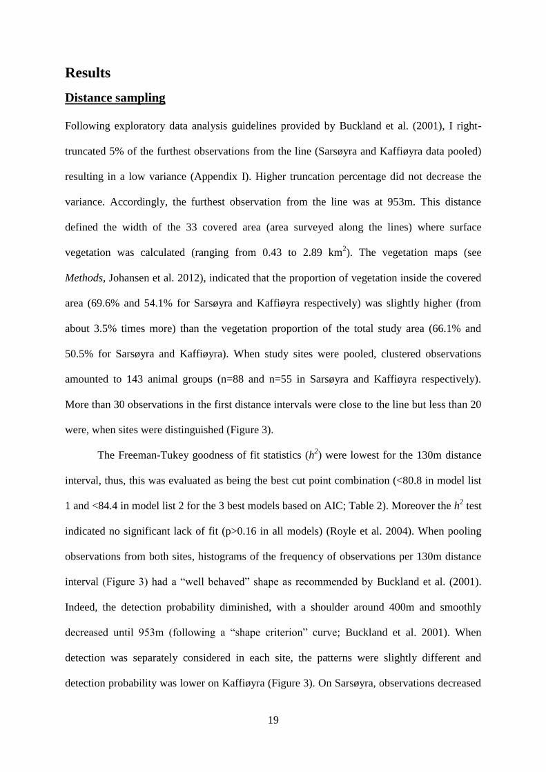
Figure 3. Distance sampling histograms of the number of clusters observed per distance
interval (numbers are given at the bottom of the bars) and the half normal detection function
probability from (a) model Hn_8 and (b and c) model Hn_21. Model Hn_8 pooled Sarsøyra
and Kaffiøyra sites for the detection function estimation while Hn_21 separated them (see text
for further details). Each observation distance to the line is plotted on the top of the detection
curve.
19
Results
Distance sampling
Following exploratory data analysis guidelines provided by Buckland et al. (2001), I right-
truncated 5% of the furthest observations from the line (Sarsøyra and Kaffiøyra data pooled)
resulting in a low variance (Appendix I). Higher truncation percentage did not decrease the
variance. Accordingly, the furthest observation from the line was at 953m. This distance
defined the width of the 33 covered area (area surveyed along the lines) where surface
vegetation was calculated (ranging from 0.43 to 2.89 km2). The vegetation maps (see
Methods, Johansen et al. 2012), indicated that the proportion of vegetation inside the covered
area (69.6% and 54.1% for Sarsøyra and Kaffiøyra respectively) was slightly higher (from
about 3.5% times more) than the vegetation proportion of the total study area (66.1% and
50.5% for Sarsøyra and Kaffiøyra). When study sites were pooled, clustered observations
amounted to 143 animal groups (n=88 and n=55 in Sarsøyra and Kaffiøyra respectively).
More than 30 observations in the first distance intervals were close to the line but less than 20
were, when sites were distinguished (Figure 3).
The Freeman-Tukey goodness of fit statistics (h2) were lowest for the 130m distance
interval, thus, this was evaluated as being the best cut point combination (<80.8 in model list
1 and <84.4 in model list 2 for the 3 best models based on AIC; Table 2). Moreover the h2 test
indicated no significant lack of fit (p>0.16 in all models) (Royle et al. 2004). When pooling
observations from both sites, histograms of the frequency of observations per 130m distance
interval (Figure 3) had a “well behaved” shape as recommended by Buckland et al. (2001).
Indeed, the detection probability diminished, with a shoulder around 400m and smoothly
decreased until 953m (following a “shape criterion” curve; Buckland et al. 2001). When
detection was separately considered in each site, the patterns were slightly different and
detection probability was lower on Kaffiøyra (Figure 3). On Sarsøyra, observations decreased

20
in two steps at 390m and 910m, with no decrease between those steps. However, on
Kaffiøyra, observations decreased earlier (from 130m) and, more regularly until 819m, yet at
520m, detection dropped more than half (from 10 to 4 clusters detected) (Figure 3).
Table 3. Parameter estimates with asymptotic standard error in parentheses from the selected
detection models of the distance sampling analysis (Table 2). σ was the detection parameter
and λ the mean density parameter on the logarithmic scale. The estimated mean abundance
and its standard deviation were bootstrapped 500 times.
Coefficient Model Hn_21 Model Hn_8
Density (ln λ)
Intercept
Vegetation
Region (Sarsøyra)
0.16 ± 0.39
2.09 ± 0.57
-0.41 ± 0.23
-0.06 ± 0.38
2.02 ± 0.53
-
Detection (ln σ)
Intercept
Region (Sarsøyra)
5.94 ± 0.11
0.42 ± 0.18
6.19 ± 0.09
-
Abundance ( )
Sarsøyra
Kaffiøyra
199 ± 33
265 ± 40
257 ± 28
174 ± 19
The most parsimonious model based on AIC was a half normal key function with
vegetation proportion and sites as additive covariates influencing density, and sites
influencing the detection function (model Hn_21, Table 2, Appendix III). The best model that
did not account for the study sites as a detection covariate was also modeled by a half normal
key function (model Hn_8, Table 2, appendix III). Only the vegetation proportion on normal
scale influenced the density estimation of model Hn_8. The AIC between those two models
was 1.92 (Table 2). However, calculating the AICc reduced the difference in parsimony
(AICc for model Hn_21= 463.65 and AICc for Hn_8= 464.17, AICc = 0.52). The proportion
of vegetated area strongly influenced the predicted density of reindeer of both model Hn_21
and Hn_8 (Table 3). Hence, if 50% of the transect surface is vegetated, for example, model
Hn_8 predicts a density of 2.59 ± 0.38 clusters/km2. If 90% of the surface is vegetated, the

21
density increases to 5.80 ± 0.91 (Appendix V). The mean number of reindeer per groups
observed with naked eyes after data truncation was . The total abundance estimates
of model Hn_21 was different and less precise than model Hn_8 (see Table 3). The estimated
abundance and standard deviation from model Hn_8 were = 256 ± 27.25 [R package
unmarked abundance ± sd] and = 174 ± 18.83 on Kaffiøyra (Table 3 and Figure 4).
State-space model time-series uncertainty
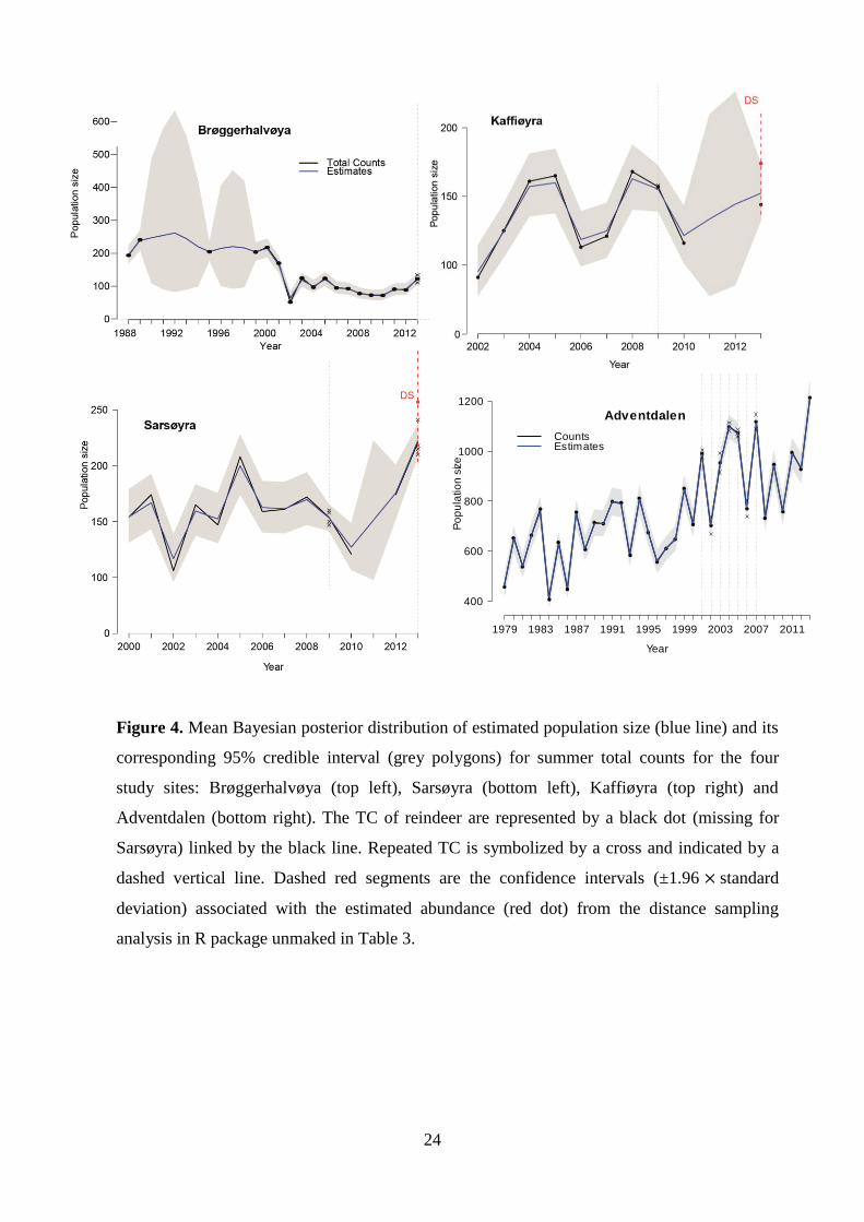
The observed total counts and estimated values from the Bayesian posterior distribution
were rather close (Figure 4), although tended to smooth extreme variations in the observed
time-series. For example, in summer 2002 on Brøggerhalvøya 65 [49:83] (posterior mean
[95% credible interval]) reindeer were estimated while 52 were counted, but the estimated
credible intervals always included the observed TC. One exception of a repeated total count
outside the CI existed in 2013, on Sarsøyra (estimate = 223 [209:237], 1st out of 4 repeats =
241 reindeer). Distance Sampling abundance estimates obtained through R package unmarked
were not included in the credible interval from the Bayesian state-space model, but the lower
part of the standard deviation was (Figure 4). One should recall that although DS density
estimates come with a wide standard deviation, one TC alone has no measure of uncertainty.
The credible intervals were reduced during years when repeated samplings were
included in the state-space model. This was illustrated by the dashed vertical lines in Figure 4.
The models were run with different data available in 2013 (Table 4) so that I could explicitly
compare the precision state estimate. Unreliable estimates were obtained when data was
missing; especially if consecutive counts were missing such as would be the case on
Kaffiøyra, if 2013 was removed. Including DS alone sharply improved the precision of the
estimates. Note that one single Total Count in 2013 gave different, but more precise results
than one single DS. When repeated total counts were conducted, standard deviation further
decreased (2009 Sarsøyra 4 repeated TC: 154 ± [142:166] CV=0.04; 2009 Kaffiøyra 2TC:
22
156 ± [140:173] CV=0.05; see table 4 for 2013). Because four TC resulted in very precise
estimates, adding DS in 2013 on Sarsøyra only improved the precision slightly. Nonetheless,
the most precise estimates integrated all data available.
The mean CV over the full Adventdalen time-series was precise (0.04). During the
seven consecutive years of independent, replicated TC in Adventdalen, the CV was slightly
improved from 0.03 (mean CV without replicates) to 0.02 (with replicates).
All four study sites were subject to strong fluctuations in population size. A major
population decrease happened on Brøggerhalvøya, Sarsøyra and Adventdalen during 2001 to
2002 (rBrøgger. = -0.95 ± [-1.26:-0.65], rSarsøyra = -0.35 ± [-0.58:-0.13] and rAdventdalen = -0.33 [-
0.40:-0.27] [posterior mean rt : CI]) (appendix IV) when the first count was performed on
Kaffiøyra with the lowest abundance estimated for that population (96 [78:115]). In all sites,
large positive growth rate followed straight after the 2002 crash (for 2003: rBrøgger.= 0.62 ±
[0.31:0.92], rSarsøyra= 0.31± [0.09:0.54], rKaffiøyra = 0.27 ± [0.04:0.50] and rAdventdalen = 0.30
[0.23:0.37], appendix VI). For example, on Brøggerhalvøya, the population approximately
doubled (TC: 52 to 125 reindeer, estimated TC: 64 [49:83] to 119 [100:141] in 2002 and
2003, respectively).
Only three counts with less than 30 reindeer from 1979-1981 on Brøggerhalvøya were
followed by seven years without censuses, which prevented MCMC chains to converge with
the upper bound of the CI up to 8500 individuals. Therefore, the time-series used in this study
started in 1988 with 194 reindeer. MCMC chains still did not converge for the 5 and 3
successive TC missing from 1990-1994 and 1996-1998 (maximum lack of convergence
obtained in 1996, Rhat=0.007, appendix IV). On Brøggerhalvøya, when summer censuses
were conducted, abundance was high from 1988 to 2001 (Figure 4). After 2003, the
population size in summer was approximately half the size compared to that before the 2002
crash. Since then, Sarsøyra has shown two peaks in 2005 and 2013. Kaffiøyra had the
23
strongest oscillating pattern despite data missing in recent years (2011 and 2012); crashes of
similar amplitudes appeared in 2006 and 2010 (r2006 = - 0.30 ± 0.11, r2010 = - 0. 25 ± 0.10), i.e.
following winters with extremely poor feeding conditions due to heavy ROS and icing
(Hansen et al. 2010, 2011).
Females reindeer with VHF collar were tracked intensively during two field season
and 97.5% (1 out of 42; 42 correspond to 19 females in summer 1999 plus 23 in summer
2000) stayed in their respective site. One animal crossed the bay between Brøggerhalvøya and
Sarsøyra in July 2000. Before the census of august 2000, 27 females (VHF marked) were
known as present in the study site. All of them were sighted during the TC. During the same
census, one out of 53 (VHF and marked) animals was counted twice (1.9%).
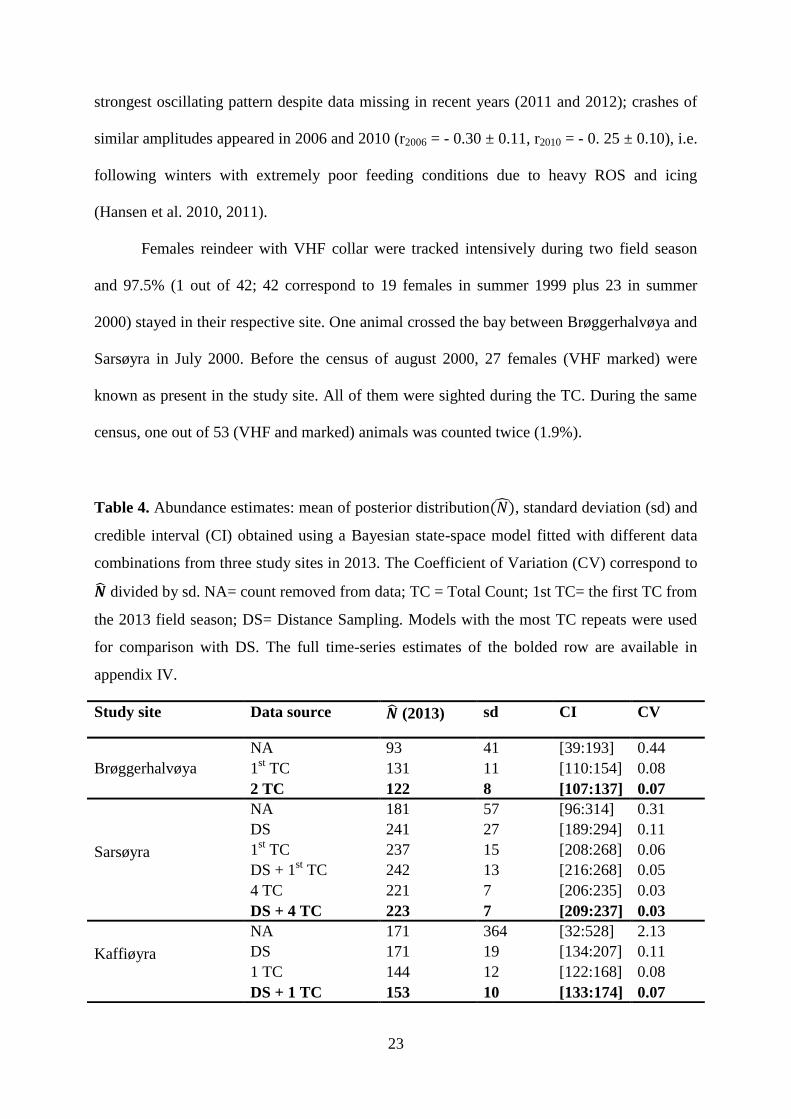
Table 4. Abundance estimates: mean of posterior distribution , standard deviation (sd) and
credible interval (CI) obtained using a Bayesian state-space model fitted with different data
combinations from three study sites in 2013. The Coefficient of Variation (CV) correspond to
divided by sd. NA= count removed from data; TC = Total Count; 1st TC= the first TC from
the 2013 field season; DS= Distance Sampling. Models with the most TC repeats were used
for comparison with DS. The full time-series estimates of the bolded row are available in
appendix IV.
Study site Data source (2013) sd CI CV
Brøggerhalvøya
NA 93 41 [39:193] 0.44
1st TC 131 11 [110:154] 0.08
2 TC 122 8 [107:137] 0.07
Sarsøyra
NA 181 57 [96:314] 0.31
DS 241 27 [189:294] 0.11
1st TC 237 15 [208:268] 0.06
DS + 1st TC 242 13 [216:268] 0.05
4 TC 221 7 [206:235] 0.03
DS + 4 TC 223 7 [209:237] 0.03
Kaffiøyra
NA 171 364 [32:528] 2.13
DS 171 19 [134:207] 0.11
1 TC 144 12 [122:168] 0.08
DS + 1 TC 153 10 [133:174] 0.07
24
Adventdalen
Year
Po
pu
latio
n s
ize
400
600
800
1000
1200
1979 1983 1987 1991 1995 1999 2003 2007 2011
CountsEstimates
Figure 4. Mean Bayesian posterior distribution of estimated population size (blue line) and its
corresponding 95% credible interval (grey polygons) for summer total counts for the four
study sites: Brøggerhalvøya (top left), Sarsøyra (bottom left), Kaffiøyra (top right) and
Adventdalen (bottom right). The TC of reindeer are represented by a black dot (missing for
Sarsøyra) linked by the black line. Repeated TC is symbolized by a cross and indicated by a
dashed vertical line. Dashed red segments are the confidence intervals (±1.96 standard
deviation) associated with the estimated abundance (red dot) from the distance sampling
analysis in R package unmaked in Table 3.

25
Discussion
In the present study, I have used time-series of strongly fluctuating sub-populations of high-
arctic Svalbard reindeer to investigate abundance uncertainties, and how uncertainties varied
between two sampling methods, TC and DS. The Bayesian state-space model made it possible
to successfully combine TC, repeated TC (within one field season) and DS in a common
framework. The inclusion of more data, even with wide standard deviation such as DS,
resulted in more precise estimates (Figure 4). In particular, the Bayesian approach enabled
direct comparisons of the precision of both sampling methods and showed that TC was more
precise than DS (Table 4). Having TC estimates as a baseline for comparison (i.e. assuming
they were close approximation to the “true” population size), emphasized that blindly
following DS model selection would have led to erroneous estimates. Finally, reindeer density
was found to be highly correlated with vegetated surface (Table 3), thus illustrating the
importance that habitat structure of the area covered by DS must be representative of the total
study site.
Extreme fluctuations are real fluctuations
Studies based on TC have demonstrated that the population size of Svalbard reindeer
fluctuates greatly between years (Solberg et al. 2001, Aanes et al. 2003, Tyler et al. 2008).
Reduced population growth is typically associated with winter “rain-on-snow” events (ROS,
see Methods) and is also more prominent when reindeer occur at high density, that is, a
negative first-order density dependence (Aanes et al. 2000, Solberg et al. 2001, Kohler and
Aanes 2004, Tyler et al. 2008, Hansen et al. 2011). In contrast, strong positive growth rates
are associated with an absence of ROS events and high quality of the grazing grounds the
previous summer (i.e. low grazing pressure and large plant biomass production linked with
high summer temperature; van der Wal and Hessen 2009; van der Wal and Stien in press).

26
Svalbard reindeer have a single offspring, so that when these conditions are met, close to all
adult female reindeer can have one calf (Øritsland 1985 reported rates up to 95%).
Nevertheless, extreme positive growth rates, such as those observed from 2002 to
2003 in Brøggerhalvøya, when the reindeer population more than doubled, were biologically
impossible if the population was isolated. Actually, partial migration occurred between sites,
especially during harsh winters (Hansen et al. 2010), influencing growth rates. This study did
not constrain growth rate or set a first-order density dependence parameter in the statistical
model, because additional uncertainties associated with the extra parameter would then be
introduced. These parameters uncertainty are not related to observational errors (Buckland et
al. 2007), thus is not related to the accuracy of the monitoring data which I concentrated on.
However it was important to ensure that migration did not impact my closure assumption
throughout the summer field season. This was supported by the 97.6% of VHF collared
females, closely tracked (every second-third days) in summer of 1999 and 2000 (Hansen et al.
2009) staying within their respective study sites. In addition, Hansen et al. (2010b) supported
that migration mainly occurred during winter.
The more information, the more precise the abundance estimate
My study is in line with Schaub and Kéry (2012) which encourages the combination of
information in hierarchical models to improve inferences in population ecology. Despite
collecting data with different sampling methods and having different uncertainties, when all
of the my available data “shared strength” (Schaub and Kéry 2012) in a common model, the
resulting estimates were more precise (Figure 4; Table 4) (see Gopalaswamy et al., 2012, for
another example of significantly improved tiger density estimates by combining two sampling
methods in the same model).
Long time-series or repeated censuses increase the precision of estimates (Sæther et al.
2007, Dennis et al. 2010, Knape et al. 2013). Likewise, in Adventdalen, the increase in

27
precision resulting from repeated TC was minimal because single annual count brought
enough information in the state-space model. Regardless of the length of the time-series, if a
count was missing, the high annual fluctuation of the reindeer population led to low precision
of abundance and growth rate estimates. Therefore, annual monitoring is crucial.
Total Counts accuracy
Total Counts accuracy can broadly vary depending on the studied species, type of landscape
and observer effort. Loison et al. (2006) calculated an index based on TC repeats of chamois
(Rupicapra sp.). In their study environment, the index was shown reliable and comparable to
capture mark recapture if enough repeats were conducted. In my study system, during a
monitoring census of August 2000, 100% (n=27) of adult female reindeer with VHF collar
were sighted. These females were tracked before the census and known as present in
Brøggerhalvøya and Sarsøyra. This demonstrated high detectability of at least adult females
when using TC. However, some repeated TC had unexpected abundance differences e.g. on
Sarsøyra in 2013 one repeat was outside the estimated CI (241 reindeer were counted while
223 [209:237] were estimated).
The main sources of errors to be accounted for were related to the observer, reindeer
fur color, and weather variability. Indeed sighting effort and the observer experience could
matter despite observers switching routes between repeats. Moreover, reindeer kept their
white winter coats until mid-July, and were easier to detect than with the dark summer fur i.e.
the count on Sarsøyra previously mentioned was the 1st TC conducted the 7
th of July 2013.
Animals were often scared off during windy days which facilitated detection but made it more
difficult to keep track of animals position. Reindeer could be missed (false negative) but also
double counted (false positive) by the same or another observer, or through animal movement
when the site needed two days (Brøggerhavøya) or more (Adventdalen) to be covered.
Systematic bias caused by false positive could only be quantified in summer 2000 where only

28
1.9% (n=53) of marked animals sighted during the census were counted twice. Nonetheless I
expected this error to also be minor other years. In any case, I considered false positive and
negative issues in our model by integrating TC in the state space model with a Poisson-
Poisson sampling.
Ahrestani et al. (2013) analyzed process and observation error in 55 globally
distributed populations of Cervus and Rangifer (27 and 28 respectively). They showed that
“more-or-less” closed populations, that have been “carefully” monitored for decades, had low
process observation error and great precision. Although process observation error cannot be
quantified in the Poisson-Poisson state-spate model, my study system followed these criteria
and supports my judgment that TC estimates, especially when repeated TC were combined,
were precise and could be assumed to have a low bias. I therefore could use TC as a reliable
baseline for the comparison of DS estimates.
Distance Sampling sources of errors: detection function
Following DS model selection blindly would have led to biased estimates. According to the
model selection, DS detection probability seemed to depend on the study site sampled (Table
3 and Figure 3. b and c). However, the similarity of landscape characteristics, methodological
and analytical protocols in the two sites did not suggest such a difference. Availability for
detection (i.e. the animal is in view) was expected to be similar inside the line transects
covered area (Buckland et al. 2004) because of the wide plain with prostrated vegetation
characteristics. Moreover, perceptibility (i.e. detection of the animal available for detection)
was also expected similar. Indeed, the same single observer covered both sites and counts
were stopped if weather prevented good visibility. In Kaffiøyra the last DS survey was
conducted on the 25-26th
of July 2013. At that time the reindeer had their darker summer fur,
which was harder to spot in the landscape. Although this could explain why fewer animals
were apparently detected from long distance on Kaffiøyra than Sarsøyra, it should not make a

29
difference in detection probability close to the line. The DS model did not account for cluster
size influencing detection even though larger groups are expected to be detected at a longer
distance (Buckland et al. 2004). This problem was reduced by data truncation so that the mean
group size was low and did not differ between sites ( 1.68 group size in Sarsøyra and
1.58 in Kaffiøyra with 5% truncation). Certainly, developing models and software that
consider quantitative covariates at the observation level would improve DS method accuracy
(see Amundson et al. in press, for an example regarding individual heterogeneity in
detection).
However, data quantity could cause differences in the fit of detection curves. Ideally, a
minimum of 60-80 observations are required to get adequate fit of the detection curve
(Buckland et al. 2001), which was largely exceeded when both sites observations were pooled
but not satisfied when Kaffiøyra was separately considered. Although both sites, combined or
not, displayed uniform distribution of cluster with a low sample size variance (Appendix I), it
is inherent that if few animal are observed, estimated density will be imprecise. Stochasticity
of the animal position is more likely to modify the shape of the histogram when sample size is
low (Figure 3). Additionally, Buckland et al., (2001) claims that the “shape criterion” is to
some extent an assumption of distance sampling. This means detection function should have a
“shoulder” shape close to the line, ensuring no movement of the animal toward or away from
the observer and that detection remains certain over a small distance from the line. This
assumption was fulfilled when data from both sites were pooled (Figure 3).
Royle et al. (2004) outlines that making “a priori judgment” about the most sensible
way to partition variance (i.e. potential predictor covariates) could minimize the possibility
that a covariate affects detection and abundance at the same time. Otherwise, the covariate
effect would be sensitive to model structure. This scenario was similar to model Hn_21 where
the study site was a covariate of both detection and density. Moreover, this model resulted in

30
a larger number of parameters than model Hn_8 (study site does not affect the detection)
(Table 4). Accordingly, the AICc showed a close to negligible difference between the two
models.
These arguments justify why I considered estimates from model Hn_8 (pooled data
from both regions to estimate the detection function) biologically reliable instead of Hn_21
(separate regions data set).
Distance Sampling source of error: habitat structure
Habitat structure could become an important source of bias if not accounted for (Pedersen et
al. 2012, Sillett et al. 2012). DS results from Hn_8 gave higher abundance estimates than TC
in both regions. The covered areas contained slightly more vegetated grounds than the total
study area, with only 3.5 % difference both in Sarsøyra and Kaffiøyra. However, density of
animals was so strongly linked to vegetation presence (Table 3) that this difference likely
explained the small overestimation (Appendix V). If the difference in vegetated surface inside
vs. outside the covered area was larger, the challenge to address both “spatial sampling and
observation error” would not have been resolved (Yoccoz et al. 2001, Sillett et al. 2012).
Anticipating such a scenario would avoid the possible need of adaptive distance sampling
(Buckland et al. 2004).
Others argue that random placement of the line is reportedly inefficient if the zone of
high density can be predicted (Buckland et al. 2004, Barabesi and Fattorini 2013). Barabesi
and Fattorini, (2013) propose a stratified sampling method where random (for an example see
Aars et al. 2009), or systematic lines (simpler to implement in the field) are placed inside
congruent polygons that cover the study site. However, systematic design cannot have
unbiased variance, yet, Fewster et al. (2009) has developed estimators of encounter rate
variance that promote such design. Definition of stratum is difficult when vegetated and non
vegetated surfaces occur along the same transect. A simple alternative would be to survey

31
additional transects until the vegetation proportion of the covered area is representative of the
total study site.
It could be argued that heterogeneity in habitats introduce bias to the assumption of
uniform distribution as well as uniform coverage probability (Buckland et al. 2004). However,
modeling detection and density as a function of habitat covariates overcomes the need to
separate density estimates into stratum that have low observations (such as non vegetated
ground) (Buckland et al. 2004). In addition, contrary to Royle et al. (2004), vegetation
coverage did not affect detectability in the model Hn_8 selected, and similar to their study,
bootstrap goodness-of-fit did not show any significant lack of fit, concluding that no other
heterogeneity should affect detection.
Future implications
The simplicity of the Svalbard tundra ecosystem should give similar count precision
between both sampling methods. The sensitivity of the DS detection function to numbers of
observations should serve as a warning to other monitoring programs using this sampling
method, especially if additional assumptions are not met. I support choosing the upper limit
outlined by Buckland et al. (2001) with a minimum number of 80 observations (for line
transect). If enough transects are surveyed to represent the total vegetation coverage, distance
sampling is a promising method to estimate reindeer density in other open tundra landscape.
The DS method demonstrated in this study will be proposed to be used by the Governor of
Svalbard, which manage Svalbard reindeer populations and conduct annual line transects. TC
might not be possible across large study areas due to high demands for resources and
logistics. Therefore reindeer abundance assessment across a wider spatial scale of the
Svalbard archipelago could combine data from sites monitored by TC and others by DS (for
an example see Aars et al. 2009). In such cases, TC should only be conducted in populations

32
assumed to be closed and with a high sampling effort to achieve the high precision as
demonstrated in this study.
More accurate estimates led to easier detection of the effects of environmental drivers
on population dynamics (Clark and Bjørnstad 2004, Knape et al. 2013), e.g. the effect of the
temperature increase in the high Arctic (Constable et al. 2014). Investigating uncertainties and
sources of error in wildlife monitoring with reliable statistical models (Buckland et al. 2007)
strengthens inferences and, thus, permit to sustainably manage an ecosystem under increasing
human pressure. The Bayesian state-space model illustrated in the present study and showed
flexibility (Clark and Bjørnstad 2004, Kery and Schaub 2012) through its adaptation to the
specificity of my study for estimating sampling methods uncertainties. Applying such analysis
with the integration of biological parameters and age structure is promising for reindeer
population dynamic studies under an increasing pressure of ROS events. Furthermore, it
would improve ecosystem dynamics understanding, and improve our ability to fully explore
the “early warning system” (Hansen et al., 2013), that is Svalbard in the light of a changing
climate.

33
Conclusion
The present study assessed uncertainty in population counts of Svalbard reindeer, leading to
useful population monitoring and management improvements. The open landscape and closed
study locations (during a field season) resulted in fairly precise abundance estimates when
monitored by TC. Nonetheless, large annual fluctuations in reindeer population size due to
environmental stochasticity, density-dependence and migration require that censuses are
conducted every year. Censuses were precise, yet quantification of counts’ bias was not
possible. However, bias was assumedly low once TC’s were integrated into the state-space
model and related to re-sightings of collard animals. Because of sample size issue, reindeer
population size would have been wrongly estimated using the DS method alone if TC could
not have been used as background information. Based on the results of this study, I strongly
recommend that DS line transects conducted in this and other wildlife systems are based on a
large number of observations (n>80) in order to obtain robust detection functions. Further,
sufficient transect lines should ensure that the habitat structure surveyed is representative of
the total study site characteristics. This study has illustrated the flexibility of the Bayesian
state-space modeling framework that maximizes the use of available data, even with wide CI,
to increase the precision of population counts. Such simple models greatly improve
population ecological inferences.

34

35
References
Aanes, R., B.-E. Saether, F. M. Smith, E. J. Cooper, P. A. Wookey, and N. A. Oritsland.
2002. The Arctic Oscillation predicts effects of climate change in two trophic levels in a
high-arctic ecosystem. Ecology Letters 5:445–453.
Aanes, R., B.-E. Sæther, E. J. Solberg, S. Aanes, O. Strand, and N. A. Øritsland. 2003.
Synchrony in Svalbard reindeer population dynamics. Canadian Journal of Zoology
110:103–110.
Aanes, R., B.-E. Sæther, and N. A. Øritsland. 2000. Fluctuations of an introduced population
of Svalbard reindeer: the effects of density dependence and climatic variation.
Ecography 23:437–443.
Aars, J., T. A. Marques, S. T. Buckland, M. Andersen, S. Belikov, A. Boltunov, and Ø. Wiig.
2009. Estimating the Barents Sea polar bear subpopulation size. Marine Mammal
Science 25:35–52.
Abadi, F., O. Gimenez, R. Arlettaz, and M. Schaub. 2010. An assessment of integrated
population models: bias , accuracy , and violation of the assumption of independence.
Ecological Society of America 91:7–14.
Ahrestani, F. S., M. Hebblewhite, and E. Post. 2013. The importance of observation versus
process error in analyses of global ungulate populations. Scientific reports 3:3125.
Amundson, C., J. A. Royle, and C. M. Handel. In press. A hierarchical model combining
distance sampling and time removal to estimate detection probability during avian point
counts. The Auk.
Barabesi, L., and L. Fattorini. 2013. Random versus stratified location of transects or points in
distance sampling: theoretical results and practical considerations. Environmental and
Ecological Statistics 20:215–236.
Brook, B. W., J. J. O’Grady, A. P. Chapman, M. A. Burgman, H. R. Resit Akcakaya, and R.
Frankham. 2000. Predictive accuracy of population viability analysis in conservation
biology. Nature 404:385–7.
Brooks, S. P., E. A. Catchpole, and B. J. T. Morgan. 2000. Bayesian animal survival
estimation. Statistical Science 15:357–376.
Buckland, S. T., D. R. Anderson, K. P. Burnham, J. L. Laake, D. L. Borchers, and L. Thomas.
2001. Introduction to distance sampling. Oxford University press, Oxford, UK.
Buckland, S. T., D. R. Anderson, K. P. Burnham, and L. Thomas. 2004. Advanced Distance
Sampling: Estimating Abundance of Biological Populations. Oxford University Press,
Oxford, UK.
Buckland, S. T., K. B. Newman, C. Fernández, L. Thomas, and J. Harwood. 2007.
Embedding Population Dynamics Models in Inference. Statistical Science 22:44–58.

36
Burnham, K. P., and D. R. Anderson. 2002. Model selection and inference: a practical
information-theoretic approach. Third edition. Springer, New York, USA.
Claeskens, G., and N. L. Hjort. 2008. Model selection and model averaging. Cambridge Univ
Press, Cambridge,UK.
Clark, J. S., and O. N. Bjørnstad. 2004. Population time series: process variability,
obaservation errors, missing values, lags, and hidden states. Ecology 85:3140–3150.
Constable, A., A. Hollowed, N. Maynard, P. Prestrud, T. Prowse, and H. Stone. 2014. Polar
regions. Chapter 28 in IPCC,2014: Climate Change 2014: Impacts, Adaptation, and
Vulnerability. Contribution of Working Group II to the Fifth Assessement Report of
Intergovernemental Panel on Climate Change. Cambridge Univ Press, Cambridge,UK.
Cressie, N., C. A. Calder, J. S. Clark, J. M. Ver Hoef, C. K. Wikle, E. Applications, S. Clark,
M. Jay, and K. Wikle. 2009. Accounting for Uncertainty in Ecological Analysis : the
Strengths and Limitations of Hierarchical Statistical Modeling. Ecological applications
19:553–570.
Dennis, B., J. M. Ponciano, and M. L. Taper. 2010. Replicated sampling increases efficiency
in monitoring biological populations. Ecology 91:610–20.
Derocher, A. E., Ø. Wiig, and G. Bangjord. 2000. Predation of Svalbard reindeer by polar
bears. Polar Biology 23:675–678.
Elvebakk, A. 1997. Tundra diversity and ecological characteristics of Svalbard. Pages 347–
359 in F. E. Wielgolaski, editor. Ecosystems of the World. Third edition. Elsevier,
Amsterdam, NL.
Fewster, R. M., S. T. Buckland, K. P. Burnham, D. L. Borchers, P. E. Jupp, J. L. Laake, and
L. Thomas. 2009. Estimating the encounter rate variance in distance sampling.
Biometrics 65:225–36.
Fiske, I. J., and R. B. Chandler. 2011. unmarked : An R Package for Fitting Hierarchical
Models of Wildlife Occurrence and Abundance. Journal of statistical software 43.
Gaillard, J.-M., M. Festa-bianchet, and N. G. Yoccoz. 2001. Not All Sheep Are Equal.
Science 292:1499–1500.
Gopalaswamy, A. M., J. A. Royle, M. Delampady, J. D. Nichols, K. U. Karanth, and D. W.
Macdonald. 2012. Density estimation in tiger populations: combining information for
strong inference. Ecology 93:1741–51.
Guillera-arroita, G., M. S. Ridout, B. J. T. Morgan, and M. Linkie. 2012. Models for species-
detection data collected along transects in the presence of abundance-induced
heterogeneity and clustering in the detection process. Methods in Ecology and Evolution
3:358–367.

37
Hansen, B. B., R. Aanes, I. Herfindal, J. Kohler, and B.-E. Sæther. 2011. Cilmate, icing, and
wild arctic reindeer: past relationships and future prospects. Ecological Society of
America 92:1917–1923.
Hansen, B. B., R. Aanes, I. Herfindal, B.-E. Sæther, and S. Henriksen. 2009a. Winter habitat–
space use in a large arctic herbivore facing contrasting forage abundance. Polar Biology
32:971–984.
Hansen, B. B., R. Aanes, and B.-E. Sæther. 2010a. Feeding-crater selection by high-arctic
reindeer facing ice-blocked pastures. Canadian Journal of Zoology 88:170–177.
Hansen, B. B., R. Aanes, and B.-E. Sæther. 2010b. Partial seasonal migration in high-arctic
Svalbard reindeer (Rangifer tarandus platyrhynchus). Canadian Journal of Zoology
88:1202–1209.
Hansen, B. B., V. Grøtan, R. Aanes, B.-E. Sæther, A. Stien, E. Fuglei, R. a Ims, N. G.
Yoccoz, and A. Ø. Pedersen. 2013. Climate events synchronize the dynamics of a
resident vertebrate community in the high Arctic. Science 339:313–315.
Hansen, B. B., I. Herfindal, R. Aanes, B.-E. Saether, and S. Henriksen. 2009b. Functional
response in habitat selection and the tradeoffs between foraging niche components in a
large herbivore. Oikos 118:859–872.
Johansen, B. E., S. R. Karlsen, and H. Tømmervik. 2012. Vegetation mapping of Svalbard
utilising Landsat TM/ETM+ data. Polar Record 48:47–63.
Kery, M., and M. Schaub. 2012. Bayesian population analysis using Winbugs: A Hierarchical
Perspective. Academic Press, Waltham, MA.
Knape, J., P. Besbeas, and P. De Valpine. 2013. Using uncertainty estimates in analyses of
population time series. Ecological Society of America 94:2097–2107.
Kohler, J., and R. Aanes. 2004. Effect of Winter Snow and Ground-Icing on a Svalbard
Reindeer Population : Results of a Simple Snowpack Model. Arctic, Antarctic, and
Alpine Research 36:333–341.
Lebreton, J.-D., and O. Gimenez. 2012. Detecting and Estimating Density Dependence in
Wildlife Populations. Wildlife Management.
Lindén, A., and J. Knape. 2009. Estimating environmental effects on population dynamics:
consequences of observation error. Oikos 118:675–680.
Loison, A., J. Appolinaire, J. Jullien, and D. Dubray. 2006. How reliable are total counts to
detect trends in population size of chamois Rupicapra rupicapra and R . pyrenaica ?
Wildlife Biology 12:77–88.
Marques, F. F. C., and S. T. Buckland. 2003. Incorporating covariates into standard line
transect analyses. Biometrics 59:924–35.

38
Marques, T. A., S. T. Buckland, R. Bispo, and B. Howland. 2012. Accounting for animal
density gradients using independent information in distance sampling surveys. Statistical
Methods & Applications 22:67–80.
Marshall, K. N., D. J. Cooper, and N. T. Hobbs. 2014. Interactions among herbivory, climate,
topography and plant age shape riparian willow dynamics in northern Yellowstone
National Park, USA. Journal of Ecology 102:667–677.
Morellet, N., J.-M. Gaillard, A. J. M. Hewison, P. Ballon, Y. Boscardin, P. Duncan, F. Klein,
and D. Maillard. 2007. Indicators of ecological change: new tools for managing
populations of large herbivores. Journal of Applied Ecology 44:634–643.
Morellet, N., F. Klein, E. Solberg, and R. Andersen. 2011. The census and management of
populations of ungulates in Europe. Pages 106–143 in R. Putman, M. Apollonio, and R.
Andersen, editors. Ungulate management in Europe: problems and practices. Cambridge
Univ Press, Cambridge,UK.
Muhlfeld, C. C., M. L. Taper, D. F. Staples, and B. B. Shepard. 2006. Observer Error
Structure in Bull Trout Redd Counts in Montana Streams: Implications for Inference on
True Redd Numbers. Transactions of the American Fisheries Society 135:643–654.
Newman, K. B., S. T. Buckland, S. T. Lindley, L. Thomas, and C. Fernández. 2006. Hidden
process models for animal population dynamics. Ecological applications 16:74–86.
Pedersen, Å. Ø., B.-J. Bårdsen, N. G. Yoccoz, N. Lecomte, and E. Fuglei. 2012. Monitoring
Svalbard rock ptarmigan: Distance sampling and occupancy modeling. The Journal of
Wildlife Management 76:308–316.
Poole, K. G., C. Cuyler, and J. Nymand. 2013. Evaluation of caribou Rangifer tarandus
groenlandicus survey methodology in West Greenland. Wildlife Biology 19:225–239.
Porteus, T., S. M. Richardsom, and J. C. Reynolds. 2011. The importance of survey design in
distance sampling: field evaluation using domestic sheep. Wildlife research 38:221–234.
Reimers, E. 1983. Mortality in Svalbard reindeer. Holarctic Ecology 6:141–149.
Rennert, K. J., G. Roe, J. Putkonen, and C. M. Bitz. 2009. Soil Thermal and Ecological
Impacts of Rain on Snow Events in the Circumpolar Arctic. Journal of Climate 22:2302–
2315.
Royle, J. A., D. K. Dawson, and S. Bates. 2004. Modeling Abundance Effects in Distance
Sampling. Ecology 85:1591–1597.
Royle, J. A., and R. M. Dorazio. 2008. Hierarchical modeling and inference in ecology.
Academic Press, San Diego, California, USA.
Schaub, M., and M. Kéry. 2012. Combining information in hierarchical models improves
inferences in population ecology and demographic population analyses. Animal
Conservation 15:125–126.

39
Seddon, P. J., K. Ismail, M. Shobrak, S. Ostrowski, and C. Magin. 2003. A comparison of
derived population estimate, mark-resighting and distance sampling methods to
determine the population size of a desert ungulate, the Arabian oryx. Oryx 37:286–294.
Sillett, T. S., R. B. Chandler, J. A. Royle, M. Kery, and S. A. Morrison. 2012. Hierarchical
distance-sampling models to estimate population size and habitat-specific abundance of
an island endemic. Ecological applications 22:1997–2006.
Singh, N. J., and E. J. Milner-Gulland. 2011. Monitoring ungulates in Central Asia: current
constraints and future potential. Oryx 45:38–49.
Solberg, E. J., P. Jordhøy, O. Strand, R. Aanes, A. Loison, B.-E. Sæther, and J. D. C. Linnell.
2001. Effects of density-dependence and climate on the dynamics of a Svalbard reindeer
population. Ecography 24:441–451.
Sutherland, W. J. 2006. Ecological Census Techniques: A Handbook. Second edition.
Cambridge Univ Press, Cambridge.
Sæther, B.-E., M. Lillegård, V. Grøtan, F. Filli, and S. Engen. 2007. Predicting fluctuations of
reintroduced ibex populations: the importance of density dependence, environmental
stochasticity and uncertain population estimates. The Journal of animal ecology 76:326–
36.
Tyler, N. J. C., M. C. Forchhammer, and N. A. Øritsland. 2008. Nonlinear effects of climate
and density in the dynamics of a fluctuating population of reindeer. Ecology 89:1675–86.
Van der Wal, R., and D. O. Hessen. 2009. Analogous aquatic and terrestrial food webs in the
high Arctic: The structuring force of a harsh climate. Perspectives in Plant Ecology,
Evolution and Systematics 11:231–240.
Van der Wal, R., and A. Stien. In press. High arctic plants like it hot: a long-term
investigation of between-year variability in plant biomass. Ecology.
Williams, B. K., J. D. Nichols, and M. J. Conroy. 2002. Analysis and management of animal
populations. Academic Press, San Diego, California, USA.
Yoccoz, N. G., J. D. Nichols, and T. Boulinier. 2001. Monitoring of biological diversity in
space and time. Trends in Ecology & Evolution 16:446–453.
Zipkin, E. F., J. T. Thorson, K. See, H. J. Lynch, E. H. C. Grant, Y. Kanno, R. B. Chandler,
B. H. Letcher, and J. A. Royle. 2014. Modeling structured population dynamics using
data from unmarked individuals. Ecology 95:22–9.
Øritsland, N. A. 1985. Svalbardreinen og Dens Livsgrunnlag. Norsk Polarinstitutt, Tromsø.

40

41
Appendix I
Sample size variance
In respect to the Poisson distribution for which , possible clumping
distribution of animals was assessed by calculating the sample size variance estimation
that was expected close to 1 (Buckland et al., 2001; p109). This corresponded to the
assumption that reindeers were randomly distributed along the different lines.
= L
represented the length of transect i, k the number of transects, the number of observations
per lines and the sum of all .
Table I. Sample size variance and its standard deviation .
Area
Sarsøyra + Kaffiøyra 206.76 14.38 1.45
Sarsøyra 124.78 11.17 1.42
Kaffiøyra 83.96 9.16 1.53

42
Appendix II
Density estimation in Distance Sampling, theoretical explanations.
The detection probability required first that the cluster was available for detection and thus
situated inside the covered area and then that it was detected by the observer (Pa). The
covered area (a) in distance sampling corresponds to the area monitored from the lines. If a
line was of length (L) and its width (ω) (including both sides of the line is of lengths 2ω),
subsequently the covered area was of 2wL m2 (meters is the measurement unit). The expected
number of clusters was issued from random and independent observations. The density
within the covered area of each partitioned line corresponded to:
=
=
Buckland et al., (2001) introduced two related functions: the detection function g( ) and the
probability density function f( ) of the perpendicular distance data from the line , related
by the relation:
=
µ was the probability to detect an animal given that it was located in the ω width and
corresponded to the area below the detection curve g( ):
µ= ω . Pa and µ =
As all observation on the line were supposed to be detected: g(0)=1
=
=
and thus
Finally (Marques and Buckland 2003),
=

43
Appendix III
Model list
Table III. Model list names implemented with the distsamp function in Unmarked R
package. Model respective detection key function (Hn= Half normal; Hz= Hazard rate, Unif=
uniform) and covariates (α = detection covariates; λ= density covariates) are reported.
Possible covariates were: the study site (site), the vegetation proportion (veg) inside the
covered area, the logarithm of the veg (ln(veg)) and the quadratic polynomial of the logarithm
value (ln(veg)2). Model list 1 corresponds to all 63 proposed models. Model list 2 correspond
to a subset of 37 models from list 1 which did not have “site” as a possible detection
covariate; models from model list 2 are highlighted in grey.
Name Hn Hz α λ
Hn x - -
Hz - -
Unif - -
Hn_1 x site -
Hn_2 x Veg -
Hn_3 x ln(veg) -
Hn_4 x ln(veg)2 -
Hn_5 x site + veg -
Hn_6 x site * veg -
Hn_7 x - site
Hn_8 x - veg
Hn_9 x - ln(veg)
Hn_10 x - ln(veg)2
Hn_11 x - site + veg
Hn_12 x - site + ln(veg)
Hn_13 x - ln(veg)2
Hn_14 x - site * veg
Hn_15 x - site * ln(veg)
Hn_16 x - ln(veg)2
Hn_17 x site site
Hn_18 x site veg
Hn_19 x site ln(veg)
Hn_20 x site site * veg
Hn_21 x site site + veg
Hn_22 x site + veg veg
Hn_23 x site + veg site
Hn_24 x site * veg veg
Hn_25 x site + veg site + veg
Hn_26 x site * veg site + veg
Hn_27 x Veg veg
Hn_28 x Veg site
Hn_29 x Veg site + veg
Hn_30 x veg site * veg
Name Hn Hz α λ
Hz_31 x site -
Hz_32 x veg -
Hz_33 x ln(veg) -
Hz_34 x ln(veg)2 -
Hz_35 x site + veg -
Hz_36 x site * veg -
Hz_37 x - site
Hz_38 x - veg
Hz_39 x - ln(veg)
Hz_40 x - ln(veg)2
Hz_41 x - site + veg
Hz_42 x - site + ln(veg)
Hz_43 x - ln(veg)2
Hz_44 x - site * veg
Hz_45 x - site * ln(veg)
Hz_46 x - ln(veg)2
Hz_47 x site site
Hz_48 x site veg
Hz_49 x site ln(veg)
Hz_50 x site site * veg
Hz_51 x site site + veg
Hz_52 x site + veg veg
Hz_53 x site + veg site
Hz_54 x site * veg veg
Hz_55 x site + veg site + veg
Hz_56 x site * veg site + veg
Hz_57 x veg veg
Hz_58 x veg site
Hz_59 x veg site + veg
Hz_60 x veg site * veg

44
Appendix IV
Table IV. Results from the Bayesian state-space model run in Winbugs for every state of the
time-series of the four sub-populations. These models combined all TC available as well as
DS estimates (see Table 1). At year t: = abundance; = growth rate. = average growth
rate and = process variance over the time-series. The mean posterior value is given with its
standard deviation = sd, 95% credible interval [2.5%:97.5%] and coefficient of variation =
CV. The chain convergence = Rhat.
Area Parameter mean sd 2.5 % 97.5 % Rhat CV
Brøgger 1988 195.89 13.89 169.40 224.00 1.001 0.07
1989 239.07 15.21 210.20 269.70 1.001 0.06
1990 247.28 101.95 109.20 487.60 1.002 0.41
1991 254.58 134.98 91.09 579.20 1.003 0.53
1992 261.74 143.62 83.07 633.10 1.004 0.55
1993 244.88 120.84 90.10 555.80 1.005 0.49
1994 220.54 81.74 99.81 421.30 1.006 0.37
1995 205.18 14.28 178.00 234.10 1.001 0.07
1996 215.10 77.32 101.10 405.50 1.007 0.36
1997 220.48 94.12 93.02 451.80 1.003 0.43
1998 216.62 82.36 96.91 420.10 1.001 0.38
1999 204.49 14.00 177.90 232.80 1.001 0.07
2000 215.39 14.24 188.50 244.30 1.001 0.07
2001 164.63 12.40 141.30 189.80 1.001 0.08
2002 64.28 8.53 48.63 82.06 1.002 0.13
2003 118.80 10.50 99.21 140.20 1.001 0.09
2004 99.97 9.32 82.50 118.90 1.001 0.09
2005 120.74 10.47 101.30 142.30 1.001 0.09
2006 96.33 9.18 79.13 115.20 1.001 0.10
2007 92.24 8.91 75.57 110.60 1.001 0.10
2008 78.71 8.11 63.62 95.36 1.001 0.10
2009 73.51 7.82 58.96 89.65 1.001 0.11
2010 73.53 7.88 58.87 89.83 1.001 0.11
2011 89.61 8.79 73.32 107.70 1.001 0.10
2012 91.14 8.89 74.52 109.30 1.001 0.10
2013 121.27 7.70 106.70 136.90 1.001 0.06 1989 0.20 0.09 0.02 0.38 1.001 - 1990 -0.04 0.37 -0.78 0.71 1.002 - 1991 -0.01 0.36 -0.72 0.69 1.005 - 1992 0.01 0.38 -0.73 0.79 1.009 - 1993 -0.04 0.37 -0.83 0.68 1.002 - 1994 -0.06 0.37 -0.86 0.64 1.001 - 1995 -0.01 0.36 -0.71 0.71 1.006 - 1996 -0.01 0.34 -0.70 0.68 1.007 - 1997 0.00 0.34 -0.69 0.69 1.003 - 1998 0.00 0.35 -0.68 0.68 1.005 - 1999 0.01 0.36 -0.71 0.74 1.001 - 2000 0.05 0.09 -0.13 0.24 1.001 - 2001 -0.27 0.10 -0.46 -0.08 1.001 - 2002 -0.95 0.15 -1.26 -0.65 1.002 - 2003 0.62 0.16 0.31 0.94 1.002 - 2004 -0.17 0.13 -0.43 0.07 1.001 - 2005 0.19 0.12 -0.05 0.44 1.001 - 2006 -0.23 0.13 -0.47 0.02 1.001 - 2007 -0.04 0.13 -0.30 0.21 1.001 - 2008 -0.16 0.14 -0.43 0.11 1.001 - 2009 -0.07 0.14 -0.35 0.21 1.001 - 2010 0.00 0.14 -0.29 0.28 1.001 - 2011 0.20 0.14 -0.08 0.48 1.001 - 2012 0.02 0.13 -0.25 0.28 1.001 - 2013 0.29 0.11 0.07 0.52 1.001 - - -0.02 0.08 -0.18 0.14 1.001 -
- 0.15 0.08 0.05 0.37 1.002 0.55 deviance - 147.65 6.55 137.00 162.40 1.001 0.04

45
Area Parameter mean sd 2.5 % 97.5 % Rhat CV
Sarsøyra
2000
2001
154.25
166.46
11.98
11.98
132.00
144.00
178.50
190.80 1.001 1.001
0.078
0.07
2002 117.30 10.67 97.45 139.10 1.002 0.09
2003 159.29 11.90 137.00 183.60 1.002 0.07
2004 152.67 11.46 130.60 175.70 1.001 0.08
2005 199.50 13.56 174.10 227.30 1.001 0.07
2006 162.20 11.61 140.00 185.70 1.001 0.07
2007 161.99 11.75 139.60 185.70 1.002 0.07
2008 169.48 12.02 146.90 194.00 1.001 0.07
2009 153.37 6.04 141.80 165.50 1.001 0.04
2010 127.33 10.56 107.10 148.60 1.002 0.08
2011 151.45 30.49 98.28 219.00 1.013 0.20
2012 175.46 12.41 151.90 200.50 1.001 0.07
2013 222.61 7.20 208.70 236.90 1.001 0.03 2001 0.08 0.10 -0.11 0.27 1.001 - 2002 -0.35 0.12 -0.58 -0.13 1.002 - 2003 0.31 0.12 0.09 0.54 1.003 - 2004 -0.04 0.10 -0.25 0.15 1.002 - 2005 0.27 0.10 0.08 0.47 1.002 - 2006 -0.21 0.10 -0.40 -0.02 1.001 - 2007 0.00 0.10 -0.19 0.20 1.001 - 2008 0.05 0.10 -0.14 0.24 1.002 - 2009 -0.10 0.08 -0.26 0.06 1.001 - 2010 -0.19 0.09 -0.37 -0.02 1.001 - 2011 0.16 0.20 -0.23 0.57 1.011 - 2012 0.16 0.20 -0.23 0.57 1.014 - 2013 0.24 0.08 0.09 0.39 1.001 - - 0.03 0.08 -0.13 0.18 1.001 2.71
- 0.08 0.05 0.02 0.21 1.001 0.69 deviance - 159.86 5.49 151.20 172.40 1.001 0.03
Area Parameter mean sd 2.5 % 97.5 % Rhat CV
Kaffiøyra
2002
2003
95.26
124.29
9.35
9.97
77.78
105.6
114.50
144.70
1.001
1.001
0.10
0.08
2004 157.14 11.63 135.60 181.20 1.001 0.07
2005 159.90 11.98 137.70 184.60 1.001 0.07
2006 118.54 10.25 99.05 139.20 1.001 0.09
2007 124.77 10.17 105.40 145.20 1.001 0.08
2008 162.81 12.07 140.40 187.70 1.001 0.07
2009 155.28 8.50 139.10 172.50 1.001 0.05
2010 121.50 10.55 101.50 142.90 1.001 0.09
2011 133.52 33.29 77.47 209.80 1.003 0.25
2012 144.31 35.41 85.42 226.40 1.003 0.25
2013 152.35 10.45 132.40 173.30 1.001 0.07 2003 0.27 0.12 0.04 0.50 1.001 - 2004 0.24 0.10 0.04 0.44 1.002 - 2005 0.02 0.10 -0.17 0.21 1.001 - 2006 -0.30 0.11 -0.53 -0.08 1.001 - 2007 0.05 0.11 -0.16 0.27 1.001 - 2008 0.27 0.11 0.06 0.48 1.001 - 2009 -0.05 0.09 -0.22 0.13 1.001 - 2010 -0.25 0.10 -0.45 -0.05 1.001 - 2011 0.07 0.24 -0.42 0.56 1.004 - 2012 0.08 0.24 -0.39 0.55 1.003 - 2013 0.08 0.24 -0.39 0.57 1.003 - - 0.04 0.09 -0.14 0.23 1.001 -
- 0.09 0.07 0.02 0.28 1.001 0.84 deviance - 93.89 4.59 87.04 104.70 1.002 0.05

46
Area Parameter mean sd 2.5 % 97.5 % Rhat CV
Adventdalen 1979 461.15 21.00 421.20 503.00 1.001 0.05
1980 647.27 25.50 598.40 698.30 1.002 0.04
1981 541.99 22.92 498.10 587.90 1.001 0.04
1982 663.25 25.28 615.30 713.90 1.002 0.04
1983 760.46 27.49 707.40 815.00 1.001 0.04
1984 418.85 20.29 379.70 459.30 1.001 0.05
1985 627.10 24.92 579.90 677.40 1.002 0.04
1986 457.83 21.24 417.10 500.60 1.002 0.05
1987 747.94 27.27 695.20 802.30 1.001 0.04
1988 611.14 24.52 564.60 660.70 1.002 0.04
1989 713.01 26.34 661.60 765.50 1.001 0.04
1990 711.62 26.36 661.10 764.50 1.001 0.04
1991 797.44 27.80 743.90 853.20 1.001 0.03
1992 790.29 28.01 736.10 845.80 1.001 0.04
1993 591.35 24.35 544.30 640.20 1.004 0.04
1994 805.45 28.00 751.40 861.70 1.002 0.03
1995 675.55 25.68 626.60 727.10 1.002 0.04
1996 560.17 22.91 516.00 606.30 1.002 0.04
1997 610.82 24.25 563.90 658.60 1.001 0.04
1998 650.66 25.43 602.30 702.00 1.001 0.04
1999 845.41 28.56 791.10 902.70 1.001 0.03
2000 713.61 26.23 662.30 765.30 1.001 0.04
2001 986.48 22.23 943.30 1031.00 1.001 0.02
2002 707.25 18.74 671.00 744.40 1.001 0.03
2003 952.97 21.77 910.40 996.00 1.001 0.02
2004 1097.38 23.35 1052.00 1144.00 1.001 0.02
2005 1070.25 23.00 1026.00 1116.00 1.001 0.02
2006 774.88 19.58 737.00 813.80 1.001 0.03
2007 1113.46 23.49 1068.00 1160.00 1.001 0.02
2008 740.38 26.81 688.80 793.90 1.001 0.04
2009 941.48 30.16 883.40 1002.00 1.001 0.03
2010 763.84 27.30 711.30 818.30 1.001 0.04
2011 991.04 31.15 931.00 1053.00 1.001 0.03
2012 931.94 30.11 873.80 991.90 1.001 0.03
2013 1211.04 34.61 1144.00 1280.00 1.001 0.03 1980 0.34 0.06 0.22 0.46 1.002 1981 -0.18 0.06 -0.29 -0.06 1.001 1982 0.20 0.06 0.09 0.31 1.001 - 1983 0.14 0.05 0.04 0.24 1.001 - 1984 -0.60 0.06 -0.72 -0.48 1.001 - 1985 0.40 0.06 0.28 0.53 1.002 - 1986 -0.32 0.06 -0.43 -0.20 1.003 - 1987 0.49 0.06 0.38 0.61 1.002 - 1988 -0.20 0.05 -0.31 -0.10 1.002 - 1989 0.15 0.05 0.05 0.26 1.002 - 1990 0.00 0.05 -0.10 0.10 1.001 - 1991 0.11 0.05 0.02 0.21 1.002 - 1992 -0.01 0.05 -0.11 0.09 1.001 - 1993 -0.29 0.05 -0.40 -0.18 1.003 - 1994 0.31 0.05 0.20 0.42 1.005 - 1995 -0.18 0.05 -0.28 -0.08 1.001 - 1996 -0.19 0.06 -0.30 -0.08 1.003 - 1997 0.09 0.06 -0.02 0.20 1.002 - 1998 0.06 0.06 -0.05 0.17 1.001 - 1999 0.26 0.05 0.16 0.36 1.001 - 2000 -0.17 0.05 -0.27 -0.08 1.001 - 2001 0.32 0.04 0.24 0.41 1.001 - 2002 -0.33 0.04 -0.40 -0.27 1.001 - 2003 0.30 0.04 0.23 0.37 1.001 - 2004 0.14 0.03 0.08 0.20 1.001 - 2005 -0.03 0.03 -0.08 0.03 1.001 - 2006 -0.32 0.03 -0.39 -0.26 1.001 - 2007 0.36 0.03 0.30 0.43 1.001 - 2008 -0.41 0.04 -0.49 -0.33 1.001 - 2009 0.24 0.05 0.15 0.34 1.001 - 2010 -0.21 0.05 -0.30 -0.12 1.001 - 2011 0.26 0.05 0.17 0.35 1.001 - 2012 -0.06 0.05 -0.15 0.03 1.001 - 2013 0.26 0.04 0.18 0.35 1.001 - 0.03 0.05 -0.07 0.13 1.001 -
0.08 0.02 0.05 0.14 1.001 0.29 deviance 404.25 8.62 389.30 423.00 1.001 0.02

47
Appendix V
Prediction of the density/abundance according to the proportion of vegetation present
Model Hn_8 issued from R package unmarked showed a strong correlation between density
of reindeer and the proportion of vegetation present. Using the function predict (Fiske and
Chandler 2011) it is possible to predict the density of reindeer with different magnitude of the
covariate. Density was predicted for every decimal from 0 to 100% of vegetation cover in
Figure V. In Table V, the same procedure was done to obtain density prediction for the total
study area (0.66 and 0.50 vegetation proportion in Sarsøyra and Kaffiøyra respectively) and
then was transformed to abundance of reindeer (see Methods). These estimates were very
close to the one obtained by TC. It supported my hypothesis that the slight difference (3.5%)
in vegetation proportion inside versus outside the covered area could explain the small
overestimation of DS estimates found in my study (Table 3). Nonetheless, care should be
taken when comparing these results because no bootstrap where conducted for the predictions
of this appendix.
Table V: (1) DS abundance predicted according to the vegetation proportion of the total study
area (not bootstrapped). (2) Results reported from Table 3; DS estimates where density was
assumed constant inside and outside the covered area. (3) Results reported from TC estimates
(four repeats for Sarsøyra) available in Table 4 and appendix IV.
Figure V: Predicted density of reindeer as a function of vegetation proportion.
Abundance Sarsøyra Kaffiøyra
(1) DS prediction 237 ± 26 150 ± 25
(2) DS extrapolation 256 ± 27 174 ± 19
(3) TC 221 ± 7 144 ± 13

48

49
Supplements
R script available online for the following topics:
1) Distance sampling analysis in R package unmarked
2) Area calculation and extraction of vegetation covariate, spatial analysis
3) Winbugs script run from R, integration of TC time-series, repeated TC and DS. An
example to measure Svalbard reindeer population size uncertainties on Sarsøyra.
Address:
https://www.dropbox.com/sh/m62r702aikgn0kh/AAB5wowezNtWmNGaR4gO8ZQGa
Articles referenced as “in press” can be requested at the following address: