Yale ICF Working Paper No. 04-20 June 14, 2004

FACTS AND FANTASIES ABOUT

COMMODITY FUTURES

Gary Gorton University of Pennsylvania

K. Geert Rouwenhorst

Yale School of Management

This paper can be downloaded without charge from the Social Science Research Network Electronic Paper Collection:

http://ssrn.com/abstract=560042

Facts and Fantasies about Commodity Futures✳

Gary GortonThe Wharton School, University of Pennsylvania

and National Bureau of Economic Research

and

K. Geert RouwenhorstSchool of Management, Yale University

This Draft: June 14, 2004

Abstract

We construct an equally-weighted index of commodity futures monthly returns over theperiod between July of 1959 and March of 2004 in order to study simple properties ofcommodity futures as an asset class. Fully-collateralized commodity futures havehistorically offered the same return and Sharpe ratio as equities. While the risk premiumon commodity futures is essentially the same as equities, commodity futures returns arenegatively correlated with equity returns and bond returns. The negative correlationbetween commodity futures and the other asset classes is due, in significant part, todifferent behavior over the business cycle. In addition, commodity futures are positivelycorrelated with inflation, unexpected inflation, and changes in expected inflation.

✳ We thank Dimitry Gupalo and Missaka Warusawitharana for research assistance, AIG Financial Productsfor financial support, Michael Crowe of the London Metals Exchange for assistance with data, Chris Lownof the Commodities Research Bureau (CRB) for assistance with the CRB data, and Frank Strohm and AmirYaron for comments and suggestions.

2

1. Introduction

Commodity futures are still a relatively unknown asset class, despite being traded in theU.S. for over 100 years and elsewhere for even longer.1 This may be because commodityfutures are strikingly different from stocks, bonds, and other conventional assets. Amongthese differences are: (1) commodity futures are derivative securities; they are not claimson long-lived corporations; (2) they are short maturity claims on real assets; (3) unlikefinancial assets, many commodities have pronounced seasonality in price levels andvolatilities. Another reason that commodity futures are relatively unknown may be moreprosaic, namely, there is a paucity of data.2

The economic function of corporate securities such as stocks and bonds, that is, liabilitiesof firms, is to raise external resources for the firm. Investors are bearing the risk that thefuture cash flows of the firm may be low and may occur during bad times, likerecessions. These claims represent the discounted value of cash flows over very longhorizons. Their value depends on decisions of management. Investors are compensatedfor these risks. Commodity futures are quite different; they do not raise resources forfirms to invest. Rather, commodity futures allow firms to obtain insurance for the futurevalue of their outputs (or inputs). Investors in commodity futures receive compensationfor bearing the risk of short-term commodity price fluctuations.

Commodity futures do not represent direct exposures to actual commodities. Futuresprices represent bets on the expected future spot price. Inventory decisions link currentand future scarcity of the commodity and consequently provide a connection between thespot price and the expected future spot price. But commodities, and hence commodityfutures, display many differences. Some commodities are storable and some are not;some are input goods and some are intermediate goods.

In this paper we produce some stylized facts about commodity futures and address somecommonly raised questions: Can an investment in commodity futures earn a positivereturn when spot commodity prices are falling? How do spot and futures returnscompare? What are the returns to investing in commodity futures, and how do thesereturns compare to investing in stocks and bonds? Are commodity futures riskier thanstocks? Do commodity futures provide a hedge against inflation? Can commodity futuresprovide diversification to other asset classes? Many of these questions have beeninvestigated by others but in large part with short data series applying to only a smallnumber of commodities.3 An exception is Bodie and Rosansky (1980), who studiedcommodity futures over the period 1950 to 1976, using quarterly data.4 In this primer we

1 Modern futures markets appear to have their origin in Japanese rice futures, which were traded in Osakastarting in the early 18th century; see Anderson, et al. (2001).2 For example, the University of Chicago Center for Research in Security Prices has no commodity futuresdata, nor does Ibbotson Associates. In addition, the well-known commodity futures indices either do notextend back very far or cannot be reproduced for various reasons.3 There is a very large literature on commodity futures. For example, see the papers collected in Telser(2000).4 Bodie and Rosansky (1980) obtained their data from a U.S. Department of Agriculture publication calledCommodities Futures Statistics and from the Journal of Commerce.

3

construct a monthly time series of an equally-weighted index of commodity futures pricesstarting in 1959. We focus on an index because we want to address the above questionswith respect to this asset class as a whole, rather than with respect to individualcommodity futures. We produce some stylized facts to characterize commodity futures.

2. The Mechanics of an Investment in Commodity Futures

A commodity futures contract is an agreement to buy (or sell) a specified quantity of acommodity at a future date, at a price agreed upon when entering into the contract – thefutures price. The futures price is different from the value of a futures contract. Uponentering a futures contract, no cash changes hands between buyers and sellers – andhence the value of the contract is zero at its inception.5

How then is the futures price determined? Think of the alternative to obtaining thecommodity in the future: simply wait and purchase the commodity in the future spotmarket. Because the future spot price is unknown today, a futures contract is a way tolock in the terms of trade for future transactions. In determining the fair futures price,market participants will compare the current futures price to the spot price that can beexpected to prevail at the maturity of the futures contract. In other words, futures marketsare forward looking and the futures price will embed expectations about the future spotprice. If spot prices are expected to be much higher at the maturity of the futures contractthan they are today, the current futures price will be set at a high level relative to thecurrent spot price. Lower expected spot prices in the future will be reflected in a lowcurrent futures price. (See Black (1976).)

Because foreseeable trends in spot markets are taken into account when the futures pricesis set, expected movements in the spot price are not a source of return to an investor infutures. Futures investors will benefit when the spot price at maturity turns out to behigher than expected when they entered into the contract, and lose when the spot price islower than anticipated. A futures contract is therefore a bet on the future spot price, andby entering into a futures contract an investor assumes the risk of unexpected movementsin the future spot price. Unexpected deviations from the expected future spot price are bydefinition unpredictable, and should average out to zero over time for an investor infutures, unless the investor has an ability to correctly time the market.

What then is the return that an investor in futures can expect to earn if he does not benefitfrom expected spot price movements, and is unable to outsmart the market? The answeris the risk premium: the difference between the current futures price and the expectedfuture spot price. If today’s futures price is set below the expected future spot price, apurchaser of futures will on average earn money. If the futures price is set above theexpected future spot price, a seller of futures will earn a risk premium.

5 This is also true at the end of each day when the value of a futures contract is reset to be zero. Gains andlosses during the day are settled by the two parties to the contract via transfers from their margin accounts.

4

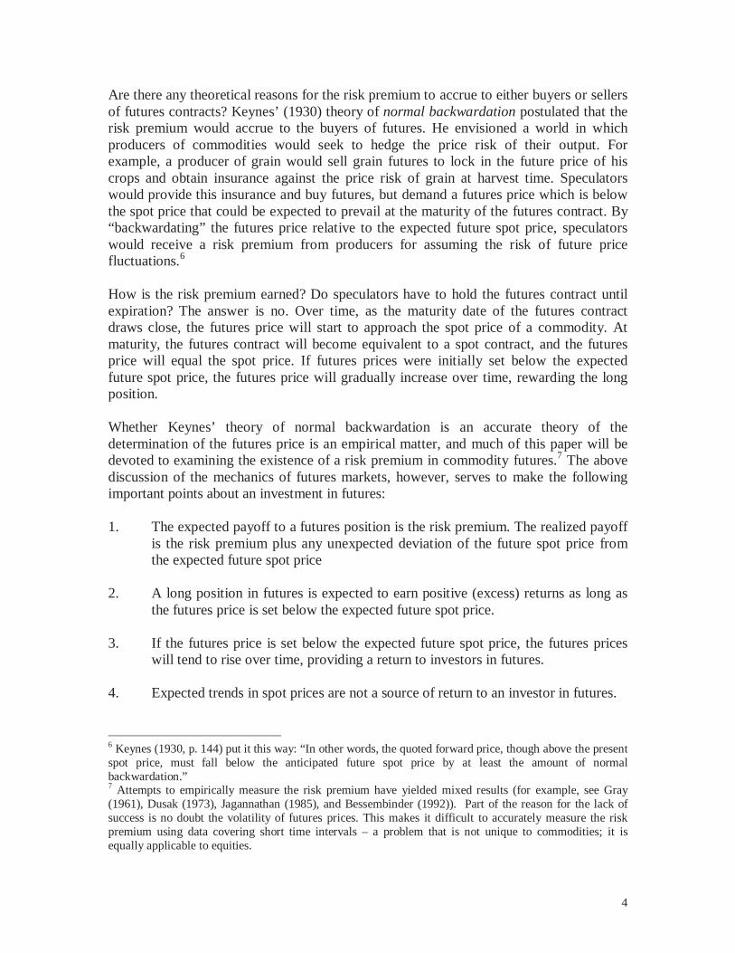
Are there any theoretical reasons for the risk premium to accrue to either buyers or sellersof futures contracts? Keynes’ (1930) theory of normal backwardation postulated that therisk premium would accrue to the buyers of futures. He envisioned a world in whichproducers of commodities would seek to hedge the price risk of their output. Forexample, a producer of grain would sell grain futures to lock in the future price of hiscrops and obtain insurance against the price risk of grain at harvest time. Speculatorswould provide this insurance and buy futures, but demand a futures price which is belowthe spot price that could be expected to prevail at the maturity of the futures contract. By“backwardating” the futures price relative to the expected future spot price, speculatorswould receive a risk premium from producers for assuming the risk of future pricefluctuations.6

How is the risk premium earned? Do speculators have to hold the futures contract untilexpiration? The answer is no. Over time, as the maturity date of the futures contractdraws close, the futures price will start to approach the spot price of a commodity. Atmaturity, the futures contract will become equivalent to a spot contract, and the futuresprice will equal the spot price. If futures prices were initially set below the expectedfuture spot price, the futures price will gradually increase over time, rewarding the longposition.

Whether Keynes’ theory of normal backwardation is an accurate theory of thedetermination of the futures price is an empirical matter, and much of this paper will bedevoted to examining the existence of a risk premium in commodity futures.7 The abovediscussion of the mechanics of futures markets, however, serves to make the followingimportant points about an investment in futures:

1. The expected payoff to a futures position is the risk premium. The realized payoffis the risk premium plus any unexpected deviation of the future spot price fromthe expected future spot price

2. A long position in futures is expected to earn positive (excess) returns as long asthe futures price is set below the expected future spot price.

3. If the futures price is set below the expected future spot price, the futures priceswill tend to rise over time, providing a return to investors in futures.

4. Expected trends in spot prices are not a source of return to an investor in futures.

6 Keynes (1930, p. 144) put it this way: “In other words, the quoted forward price, though above the presentspot price, must fall below the anticipated future spot price by at least the amount of normalbackwardation.”7 Attempts to empirically measure the risk premium have yielded mixed results (for example, see Gray(1961), Dusak (1973), Jagannathan (1985), and Bessembinder (1992)). Part of the reason for the lack ofsuccess is no doubt the volatility of futures prices. This makes it difficult to accurately measure the riskpremium using data covering short time intervals – a problem that is not unique to commodities; it isequally applicable to equities.

5

To further illustrate these points, consider a stylized example, adapted from Weiser(2003). The example is displayed in Figure 1 below. Assume that the spot price of oil is$30 a barrel and that market participants expect the price of oil to be $27 in three months.In order to entice investors into the market, the futures price is set at $25, which is adiscount to the expected future spot price. The difference between the futures price andthe expected future spot price, or $2, is the risk premium that the investor expects to earnfor assuming short-term price risk.

Now suppose that at the time the contract expires, oil is trading at the expected price of$27. An investor in physical commodities, who cares about the direction of spot prices,has just lost $3 (i.e., $30 - $27). An investor in the futures contract, however, would havegained the difference between the final spot price of $27 and the initial futures price of$25, or $2.

The example above, and the figure, examine the case where the expected future spot priceof $27 is, in fact, realized. But suppose the expectation of a price of $27 is not realizedand instead the final spot price turns out to be $26. Then the realized return to theinvestor would be $1. This realized return can be broken down into the risk premium($27 - $25 = $2), less the difference between the final spot price and the expected price($26 - $25 = $1).

Figure 1: Futures versus Spot returns

Inception Expiration

Investor Expects to EarnRisk Premium

Market ParticipantsSpot Prices to Decline

Current Spot Price

Spot/Futures Converge at Expiration

Expected Spot Price at Expiration

Futures Price at Inception

6

The remainder of the paper will be devoted to empirical evidence on the historicalperformance of commodity futures as an asset class. One final remark needs to be maderegarding the calculation of futures returns. At the beginning of this section, we explainedthat the value of a futures contract is zero at origination, and does not require any cashoutlay for either the long or the short position. In practice, both the long and shortposition will have to post collateral that can be used to settle gains and losses on thefutures position over time. The collateral is typically only a fraction of the notional valueof the futures position, which implies that a futures position can involve substantialleverage.

In order to draw a meaningful comparison between the performance of futures and otherasset classes, we need to control for leverage when calculating futures returns. We makethe assumption that futures positions will be fully collateralized. When an investor buys acontract with a futures price of $25, we will assume that the investor simultaneouslyinvests $25 in T-bills. The total return earned by the investor over a given time period,will therefore be the change in the futures price and the interest on the $25 (calculateddaily), scaled by the $25 initial investment.

3. An Equally-Weighted Index of Commodity Futures

To investigate the long-term return to commodity futures we constructed an equally-weighted performance index of commodity futures. The source of our data is a databasemaintained by the Commodities Research Bureau, which has daily prices for individualfutures contracts since 1959. We append these data with data from the London MetalsExchange. A detailed description of the data is given in Appendix 1, but a few generalcomments are in place.

Our index potentially suffers from a variety of selection and survivorship biases. First,the CRB database mostly contains data for futures contracts that have survived untiltoday, or were in existence for extended periods during the 1959-2004 period. Manycontracts that were introduced during this period, but failed to survive, are not included inthe database. It is not clear how survivorship bias affects the computed returns to afutures investment. Futures contracts fail for lack of interest by market participants, i.e.lack of trading volume. See Black (1986) and Carlton (1984). While this may becorrelated with the presence of a risk premium, the direction of the bias is not as clear cutas would be the case of the calculation of an equity index. Among other reasons, stocksdo not survive because of bankruptcy, and excluding bankrupt firms would create astrong upward bias in the computed returns. Second, in order to avoid double counting ofcommodities, we selected contracts from a single exchange for inclusion in our index,even though a commodity might be traded on multiple exchanges. We based our selectionon the liquidity of the contract, and it is therefore subject to a selection bias that may ormay not be correlated with the computed returns. Finally, for each commodity, there aremultiple contracts listed that differ by maturity. On each day, we selected the contractwith the nearest expiration date (the shortest contract) for our index, unless the contract

7

expired in that month, in which case we would roll into the next contract. In each month,we therefore hold the shortest futures contract that will not expire in that month.8

The performance index is computed as follows: at the beginning of each month we holdone dollar in each commodity futures contract. (If the futures price is $25, we hold 1/25th

of a contract). At the same time we purchase $1 in T-bills for every contract that theindex invests in. The index is therefore “fully collateralized” by a position of T-bills. Thecontracts are held until the end of the month, at which time we rebalance the index toequal weights. More detail is contained in Appendix 1.

There are many different ways in which we could have weighted individual commodityfutures in our index.9 By analyzing the returns of an equally-weighted index ofcommodity futures we can make statements about “how the average commodity futurebehaves during the average time period.”

4. The Historical Returns on Commodities: Spot Prices, Collateralized Futures, andInflation

We now turn to the empirical evidence on spot and future returns. What is the averagereturn to commodity futures? Does the collateralized futures position outperform the spotreturn for the “average commodity future”? Figure 2a compares the equally-weightedtotal return index of commodity futures to an equally-weighted portfolio of spotcommodities between 1959 and 2004. Both indices have been adjusted for inflation bydeflating each series by the consumer price index (CPI). The index of commodity spotprices simply tracks the evolution of the spot prices, and ignores all costs associated withthe holding of physical commodities (storage, insurance, etc). It is therefore an upperbound on the return that an investor in spot commodities would have earned. The mainconclusions from examination of the figure are that:

1. There are large differences between the historical performance of spot commodityprices and collateralized commodity futures returns. The historical return to aninvestment in commodity futures has far exceeded the return to a holder of spotcommodities.

2. Both commodity spot prices and commodity futures returns have outpaced inflation.

8 The rolling itself is not a source of return. Because the futures price adjusts continuously, and gains andlosses are settled daily, a futures contract has zero value at the end of each day. Even though a distantfutures contract may have a different futures price than a near contract, the exchange of one for another hasno cash flow implications.9 The popular traded indices of collateralized commodity futures sometimes use (a combination of)production and liquidity data as the basis for calculating weights (e.g., the Dow Jones AIG CommodityIndex and the Goldman Sachs Commodity Index). The Reuters-CRB index uses equal weights, but does notrebalance like our index.

8

Figure 2a

Figure 2b

Commodities Inflation Adjusted Performance 1959/7-2004/3Spot versus Equally-weighted Collateralized Futures Index 1959/7 = 100

0

250

500

750

1000

1250

1500

1750

Jul-59 Jul-63 Jul-67 Jul-71 Jul-75 Jul-79 Jul-83 Jul-87 Jul-91 Jul-95 Jul-99 Jul-03

Commodity Futures

Commodity Spot Prices

Commodities Inflation Adjusted Performance 1959/7-2004/3 Log ScaleSpot versus Equally-weighted Collateralized Futures Index 1959/7 = 100

10

100

1000

10000

Jul-59 Jul-63 Jul-67 Jul-71 Jul-75 Jul-79 Jul-83 Jul-87 Jul-91 Jul-95 Jul-99 Jul-03

Commodity Futures

Commodity Spot Prices

9

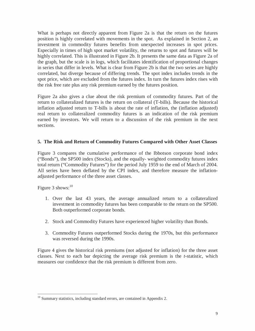
What is perhaps not directly apparent from Figure 2a is that the return on the futuresposition is highly correlated with movements in the spot. As explained in Section 2, aninvestment in commodity futures benefits from unexpected increases in spot prices.Especially in times of high spot market volatility, the returns to spot and futures will behighly correlated. This is illustrated in Figure 2b. It presents the same data as Figure 2a ofthe graph, but the scale is in logs, which facilitates identification of proportional changesin series that differ in levels. What is clear from Figure 2b is that the two series are highlycorrelated, but diverge because of differing trends. The spot index includes trends in thespot price, which are excluded from the futures index. In turn the futures index rises withthe risk free rate plus any risk premium earned by the futures position.

Figure 2a also gives a clue about the risk premium of commodity futures. Part of thereturn to collateralized futures is the return on collateral (T-bills). Because the historicalinflation adjusted return to T-bills is about the rate of inflation, the (inflation adjusted)real return to collateralized commodity futures is an indication of the risk premiumearned by investors. We will return to a discussion of the risk premium in the nextsections.

5. The Risk and Return of Commodity Futures Compared with Other Asset Classes

Figure 3 compares the cumulative performance of the Ibbotson corporate bond index(“Bonds”), the SP500 index (Stocks), and the equally- weighted commodity futures indextotal return (“Commodity Futures”) for the period July 1959 to the end of March of 2004.All series have been deflated by the CPI index, and therefore measure the inflation-adjusted performance of the three asset classes.

Figure 3 shows:10

1. Over the last 43 years, the average annualized return to a collateralizedinvestment in commodity futures has been comparable to the return on the SP500.Both outperformed corporate bonds.

2. Stock and Commodity Futures have experienced higher volatility than Bonds.

3. Commodity Futures outperformed Stocks during the 1970s, but this performancewas reversed during the 1990s.

Figure 4 gives the historical risk premiums (not adjusted for inflation) for the three assetclasses. Next to each bar depicting the average risk premium is the t-statistic, whichmeasures our confidence that the risk premium is different from zero.

10 Summary statistics, including standard errors, are contained in Appendix 2.

10

Figure 3

Figure 4

Stocks, Bonds, and CommoditiesInflation Adjusted Performance 1959/7-2004/3

0

250

500

750

1000

1250

1500

1750

2000

Jul-59 Jul-63 Jul-67 Jul-71 Jul-75 Jul-79 Jul-83 Jul-87 Jul-91 Jul-95 Jul-99 Jul-03

Bonds

Stocks

Commodities

Risk Premium by Asset ClassAnnualized monthly excess returns 1959/7-2004/7

0%

1%

2%

3%

4%

5%

6%

Stocks Bonds Commodity Futures

t = 2.36

t = 1.48

t = 2.84

11

Two observations stand out:

1. The historical risk premium on Commodity Futures has been positive at about 5%during the 1959-2004 period, and significant in a statistical sense (t-statistic = 2.84)

2. The historical risk premium on Commodity Futures is about the same as the riskpremium on Stocks (SP500), and more than double the risk premium of Bonds.

As pointed out in Section 2, there has been much debate among economists about theexistence of a risk premium in commodity futures. Keynes (1930) and Hicks (1939)assumed that hedgers outnumber speculators in the futures markets, which was the basisfor the theory of normal backwardation. The estimated risk premium in Figure 4 is notonly consistent with the theory of normal backwardation, but – more importantly – it alsoshows that the risk premium has been economically large and statistically significant.

Our commodities total return index covers a period of more than 40 years, and isdiversified across many commodities. As such it provides a unique opportunity toexamine the risk premium across a variety of commodities and time periods.

Figure 5 compares the performance (unadjusted for inflation) of stocks, bonds andcommodities in the familiar average return – standard deviation diagram.

Figure 5

Risks and Return of Commodity FuturesAnnualized monthly returns, 1959/7-2004/3

0%

2%

4%

6%

8%

10%

12%

14%

16%

5% 6% 7% 8% 9% 10% 11% 12%

Average Return

StandardDeviation

Tbills

Bonds

Commodities

Stocks

12

The volatility of the equally-weighted Commodity Futures total return is slightly belowvolatility of the SP500. So, the Sharpe Ratio has been slightly higher for CommodityFutures than for Stocks (also indicated by the higher t-statistics in Figure 4).

Financial returns are not completely characterized by the mean return and the standarddeviation of returns. This is because, as is well known, the returns on financial securitiesare not normally distributed, but rather have “fat tails” compared to the NormalDistribution. This is also true of commodity futures. Commodity futures returns arepositively skewed; stock returns are negatively skewed. Bodie and Rosansky (1980), andothers, also note that commodity futures returns are considerably positively skewedcompared to stock returns.

This is further illustrated in Figure 6, which compares the empirical distribution ofmonthly returns for the SP500 and our equally-weighted commodity futures indexbetween 1959 and 2004.

Figure 6

Three observations stand out:

1. Commodity Futures and Stocks have about the same average return, but thestandard deviation of stock returns is slightly higher.

2. The return distribution of equities has negative skewness, while the distribution ofcommodity returns has positive skewness. This means that, proportionally,equities have more weight in the left tail of the return distribution whilecommodities have more weight in the right tail.

Stocks and Commodity FuturesEmpirical Distributions of Monthly Returns 1959/7 - 2004/3

0%

5%

10%

15%

20%

25%

30%

<-14 .9

%

-13.2

%

-11 .6

%

-9.9

%-8

.3%

-6.6

%-5

.0%

-3.3

%

-1.6

%0 .0

%1.7

%3.3

%5.0

%6.6

%8.3

%9.9

%

11 .6%

13 .3%

14.9%

>15 .5%

Relative Frequency

StocksCommodity Futures

13

3. Both the return distributions have positive excess kurtosis, that is, they are“peaked” relative to the normal distribution.

The slightly higher variance of equities, and the opposite skewness, together imply thatequities have more downside risk relative to commodities. For example, the 5% tail of theempirical distribution of equities occurs at –6.56% compared to –4.05% for commodities.From the perspective of risk management, an important question is whether these tailevents occur simultaneously for both assets, or in isolation. We will turn to the questionof correlation next.

6. The Correlation of Commodities with Other Asset Classes

We examine the correlation of Commodity Futures returns with Stocks and Bonds overvarious investment horizons. In addition to monthly returns, we report correlationscomputed using overlapping returns over quarterly, annual and 5-year intervals. Becauseasset returns are volatile, examining correlation over longer holding periods may revealpatterns in the data that are obscured by short-term price fluctuations. Figure 7 illustratesthe correlations of Commodity Futures returns with Stocks, Bonds, and Inflation over theperiod between 1959 and 2004:

Figure 7

monthlyquarterly

annual

5-year

Stocks

Bonds

Inflation

-60%

-40%

-20%

0%

20%

40%

60%

horizon

Correlation with Commodity Futures

Overlapping return data 1959/7-2004/3

14

1. Over all horizons – except monthly – the equally-weighted Commodity Futurestotal return is negatively correlated with the return on the SP500 and long-termbonds. This suggests that Commodity Futures are effective in diversifying equityand bond portfolios.

2. The negative correlation between Stocks and Bonds tends to increase with theholding period. This suggests that the diversification benefits of CommodityFutures tend to be larger at longer horizons.

3. Commodity Futures returns are positively correlated with inflation, and thecorrelation is larger at longer horizons. Because Commodity Future returns arevolatile relative to inflation, longer-term correlations better capture the inflation-properties of a commodity investment.

In Figure 5 we showed that equities contain more downside risk than CommodityFutures. So it is important to ask whether the negative correlation between equities andCommodity Futures holds up when equity returns are low – a time when diversification isespecially valuable. We examined the returns to Commodity Futures during the monthsof lowest equity returns. The results are given in Figure 8a and 8b. Figure 8a shows theequity returns during the 5% of worth months of lowest performance. Figure 8bconcentrates on the lowest 1% of realized equity returns. The figures show the following:

1. During the 5% of the months of worst performance of equity markets, whenstocks fell on average by 9.18%, Commodity Futures experienced a positivereturn of 1.43%, which is slightly more than the full sample average return of0.88% per month.

2. During the 1% of months of lowest performance of equity markets, whenequities fell on average by 13.87%, Commodity Futures returned an averageof 2.32%.

It seems that the diversification benefits of Commodity Futures work well when they areneeded most. Consistent with a negative correlation, Commodity Futures earn aboveaverage returns when stocks earn below average returns

15

Figure 8: Commodity Futures Returns When Stock Returns are Low

– 6.56%

– 10.82%

Bottom 5 % of Equity Returns:Average Equity Return in Tail = – 9.18%

Average Commodity Futures Return in Tail = 1.43 %

Bottom 1% of Equity Returns:Average Equity Return in Tail = – 13.87%Average Commodity Futures Return in Tail = 2.32 %

Bottom 5% Equity Returns

Average Equity Return in Tail = – 9.18%

– 6.56%

Average Commodity Futures Return in Tail = 1.43 %

mean = 0.92 %

stdev = 4.30 %

16

7. Commodity Futures Returns and Inflation

Investors ultimately care about the real purchasing power of their returns, which meansthat the threat of inflation is a concern for investors. Many traditional asset classes are apoor hedge against inflation – at least over short and medium-term horizons.

Bonds are nominally denominated assets, and their yields are set to compensate investorsfor expected inflation over the life of the bond. When inflation is unexpectedly higherthan the level investors contracted for, the real purchasing power of the cash flows willfall short of expectations. To the extent that unexpected inflation leads to revisions offuture expected inflation, this loss of real purchasing power can be significant.

There are reasons to expect equities to provide a better hedge than bonds against inflation– at least in theory. After all, stocks represent claims against real assets, such asfactories, equipment, and inventories, whose value can be expected to hold pace with thegeneral price level. However, firms also have contracts with suppliers of inputs, labor andcapital, that are fixed in nominal terms and hence act very much like nominal bonds. Inaddition, (unexpected) inflation is often not neutral for the real economy. Unexpectedinflation is associated with negative shocks to aggregate output, which is generally badnews for equities. (See Fama (1981).) In sum, the extent to which stocks provide a hedgeagainst inflation is an empirical matter.

Figure 7 suggested that commodity futures might be a much better inflation hedge thanstocks or bonds. First, because commodity futures represent a bet on commodity prices,they are directly linked to the components of inflation. Second, because futures pricesinclude information about foreseeable trends in commodity prices, they rise and fall withunexpected deviations from components of inflation. This is exactly why futures do wellwhen stocks and bonds perform poorly.

Figure 9 compares the correlations of stocks, bonds, and commodities with inflation. Asbefore, correlations are computed over various investment horizons.

Several observations stand out from Figure 9:

1. Commodity Futures have an opposite exposure to inflation compared to Stocks andBonds. Stocks and Bonds are negatively correlated with inflation, while thecorrelation of Commodity Futures with inflation is positive at all horizons.

2. In absolute magnitude, inflation correlations tend to increase with the holding period.The negative inflation correlation of Stocks and Bonds and the positive inflationcorrelation of Commodity Futures are larger at return intervals of 1 and 5 years thanat the monthly or quarterly frequency.

17

Figure 9

Our previous discussion suggested that stocks, and especially bonds, can be sensitive tounexpected inflation. In order to measure unexpected inflation, a model of expectedinflation is needed. For this purpose we choose a very simple method that has been usedby others in the past (e.g., see Fama and Schwert (1977) and Schwert (1981)). The short-term T-bill rate is a proxy for the market’s expectation of inflation, if the expected realrate of interest is constant over time. Consequently, unexpected inflation can be measuredas the actual inflation rate minus the nominal interest rate (which was known ex ante).

Because inflation is persistent over time, unexpected inflation often causes marketparticipants to revise their estimates of future expected inflation. The change in expectedinflation can be measured by the change in the nominal interest rate. This is not

monthlyquarterly

annual5-year

Stocks

Bonds

Commodities

-60%

-40%

-20%

0%

20%

40%

60%

Horizon

Correlation with Inflation Overlapping return data 1959/7-2004/3

18

necessarily perfectly correlated with the unexpected inflation rate since investors may usemore information than just the current rate of inflation to revise their expectations offuture inflation.11

Figure 10

11 Following the large literature on inflationary expectations, we choose the 30-day and 90-day T-bill yieldas our measure of expected inflation for the next month, and quarter. See Fama and Schwert (1977) andSchwert (1981) for a discussion.

InflationUnexpected Inflation

Change ExpectedInflation

Stocks

Bonds

Commodities

-60%

-40%

-20%

0%

20%

40%

60%

Correlation with Inflation ComponentsOverlapping quarterly return data 1959/7-2004/3

19

Figure 10 illustrates the correlations of Stocks, Bonds, and Commodity Futures returnswith the components of inflation. These observations stand out:

1. The negative sensitivities of Stocks and Bonds to inflation stem mainly fromsensitivities to unexpected inflation. The correlations with unexpected inflationexceed the raw inflation correlations.

2. Commodity Futures are also more sensitive to unexpected inflation, but (again) inthe opposite direction.

3. Stock returns and (especially) Bond returns are negatively influenced by revisionsabout future expected inflation. Revisions about future inflationary expectationsare a positive influence on Commodity Futures returns.

4. Unreported results show that these patterns in the exposures to unexpectedinflation are stronger at the quarterly horizon than at the monthly horizon.

Commodity Futures returns are negatively correlated with stock returns. CommodityFutures have opposite exposures to unexpected inflation from Stocks and Bonds. It istempting to put both together and ask: does the opposite exposure to unexpected inflationaccount for the negative correlation between Commodity Futures and Stocks and Bonds?Preliminary findings suggest that this only part of the story behind the negativecorrelations. If we isolate the portion of the returns of commodity futures, stocks andbonds that is unrelated to unexpected inflation and examine the correlations again, wefind that the residual variation of commodity futures and stocks or bonds continue to benegatively correlated.12 At the quarterly horizon, the correlation between futures andstocks increases from –0.13 to –0.09, while for bonds the correlation increases from –0.22 to –0.18. In other words there are additional factors that drive the negativecorrelation between futures returns and stocks and bonds. The next section describes oneof these sources: business cycle variation.

8. Commodity Returns over the Business Cycle.

Modern finance theory identifies two components to asset returns: a systematiccomponent and a nonsystematic, or idiosyncratic, component. Holding a portfolio ofmany different securities can diversify idiosyncratic components. But, the systematiccomponent corresponds to movements in the market as a whole, and so is viewed asnondiversifiable. The nondiversifiable component, associated with beta in the CapitalAsset Pricing Model, also corresponds to the business cycle since business cycle risk isnondiversifiable. Stock and bond returns are negative in (the early phase of) recessions,in particular.

12 In other words, we examine the correlation of regression residuals from regressions of each asset class’returns on unexpected inflation.

20

Commodity future returns and equity returns are negatively correlated at quarterly,annual, and five-year horizons. This means that commodity futures are useful in creatingdiversified portfolios, with respect to the idiosyncratic component of returns.

But, importantly, there is also evidence of another “diversification effect.” Commodityfutures have a feature quite unique to this asset class, namely, commodity futures havesome power at diversifying the systematic component of risk – the part that is notsupposed to be diversifiable! Weiser (2003) reports that commodity futures returns varywith the stage of the business cycle.13 In particular commodity futures perform well in theearly stages of a recession, a time when stock returns generally disappoint. In later stagesof recessions, commodity returns fall off, but this is generally a very good time forequities.

Figure 11: Business Cycle Phases

-1.5

-1

-0.5

0

0.5

1

1.5

1 6 11 16 21 26 31 36 41 46 51 56 61 66 71 76 81 86 91 96 101

106

111

116

121

126

131

136

141

146

151

156

161

166

171

176

181

186

191

196

201

206

211

216

221

226

231

236

241

246

251

256

261

266

271

276

281

286

291

296

301

306

311

316

321

326

331

336

341

346

351

356

361

366

371

376

381

386

391

396

401

406

411

416

421

426

431

436

441

446

451

456

461

466

471

476

481

486

491

496

501

506

511

516

521

526

531

536

541

546

551

556

561

566

571

576

581

586

591

596

601

606

611

616

621

626

NBER peak

NBER trough

Late Expansion Early Recession

Late Recession

Early Expansion

Figure 11 displays a business cycle, where the National Bureau of Economic Research(NBER) peak and trough are identified.14 The NBER identifies peaks and troughs, but thefigure further divides the cycle into phases. Phases are identified by dividing the numberof months from peak to trough (trough to peak) into equal halves to indicate EarlyRecession and Late Recession (Early Expansion and Late Expansion). Clearly, the Early

13 Weiser (2003) looks at the period 1970-2003, and determines business cycle dating in terms of the rate ofchange of the quarterly GDP growth rate. Vrugt (2003) also analyzes the period 1970-2003. He usesNational Bureau of Economic Research (NBER) business cycle dating, and divides the business cycle intophases. We have used Vrugt’s (2003) figure to show the phases.14 The NBER is a private, nonprofit, economic research consortium, which dates business cycles in the U.S.by identifying business cycle peaks and troughs. See http://www.nber.org/cycles.html .

21

and Late Expansion phases correspond to an economic expansion, while the Early andLate Recession phases correspond to a recession.

In order to analyze the behavior of commodity futures over the business cycle, we wouldlike to include as many business cycles as possible. The equally weighted commodityfutures index that we constructed, detailed in Appendix 1, is useful for this.

Starting in 1959 allows us to analyze seven full business cycles, more than Weiser (2003)and Vrugt (2003). (The relevant NBER business cycle chronology for this period isshown in Appendix 3.)

Average annualized (monthly) returns for the major asset classes are given below inFigures 12 and 13. We examine the returns during expansions and recessions, and for thefour phases of the cycle.

Figure 12

OverallExpansion

Recession

Stocks

Bonds

Commodities

0.0%

2.5%

5.0%

7.5%

10.0%

12.5%

15.0%

Average Returns over Business CycleAnnualized Monthly Returns 1959/7 - 2004/3

Looking at Figure 12, note the following:

1. Over the period July 1959 through March 2004, average monthly annualized returnson the S&P and the equally-weighted commodity futures total return are remarkablysimilar, 10.8% and 10.5%, respectively.

22

2. They are also remarkably similar over expansions, 12.8% on the S&P and 12.9% onthe equally weighted commodity futures. Over recessions, the average monthlyannualized returns for the S&P and the equally weighted commodity futures are 1.7%and 0.5%.

Based on these two observations, stocks and the commodity futures index appear to bevery similar. But, these similarities obscure an important difference when the businesscycle is examined in more detail in Figure 13.

Figure 13

EarlyExpansion Late

Expansion EarlyRecession Late

Recession

Stocks

Bonds

Commodities

-20%

-10%

0%

10%

20%

30%

Average Returns over Business CycleAnnualized Monthly Returns 1959/7 - 2004/3

3. During the Early Recession phase the returns on both stocks and bonds are negative, -15.5% and –2.9% respectively. But, the return on commodity futures is a positive3.5%. During the Late Recession phase the signs of the returns reverse, stocks andbonds are positive, while commodity futures are negative.

4. The diversification effect is not limited to the early stages of recessions. Wheneverstock and bond returns are below their overall average, in the Late Expansion andEarly Recession phases, commodity returns are positive and commodities outperformboth stocks and bonds.

The last two conclusions are not evident if the sample is confined to the period 1990-2004, a period which does not cover enough business cycles.

To explore this business cycle diversification effect just a bit further we ask whether thereare certain individual commodity futures that are responsible for the result. A further

23

breakdown by stage of the business cycle for individual commodity futures is shownbelow.

Stock, Bond and Individual Commodity Futures Performance over the BusinessCycle, 7/1959 – 3/2004*

Avg. Monthly Annualized% Returns

Phase Avg.

Data SeriesStartingDate of

Data SeriesOverall

Avg.Expansion

Avg.Recession

Avg.Late

ExpansionEarly

ExpansionEarly

RecessionLate

Recession

Inflation 07/01/59 4.2% 4.0% 6.5% 4.6% 3.6% 7.6% 5.4%S&P Total Return 07/01/59 11.1% 13.1% 1.7% 10.4% 18.1% -15.5% 17.3%Corporate Bonds TR 07/01/59 7.7% 7.2% 12.1% 3.6% 11.5% -2.9% 25.7%Eq. Wtd Futures TR 07/01/59 11.0% 13.4% 0.9% 16.9% 7.4% 4.3% -1.7%Equal Wt Spot 07/01/59 8.7% 10.8% -2.0% 12.3% 7.7% 0.7% -3.7%Eq Wt Energy Futures 11/30/78 19.2% 14.7% -0.8% 17.1% 6.0% 5.4% -7.8%Eq Wt NonEnergyFutures

07/01/59 10.2% 10.2% -12.9% 15.7% 7.2% 1.8% 0.5%

Eq Wt Industrial MetalsFutures

07/01/59 15.4% 18.4% 6.3% 27.2% 3.5% 15.7% -29.8%

Eq Wt IndustrialNonMetals Futures

01/05/60 7.7% 10.9% -14.9% 13.5% 8.7% -5.4% -13.4%

Eq Wt Precious MetalsFutures

11/06/63 9.4% 11.5% -8.7% 17.9% 2.3% 0.1% -10.5%

Eq Wt Animal ProductsFutures

09/19/61 11.8% 15.1% -7.7% 17.9% 9.0% -3.6% 5.8%

Eq Wt Other FoodFutures

07/01/59 9.9% 6.4% 20.3% 11.7% 14.3% 15.7% 0.2%

Eq Wt Grain andProducts Futures

07/01/59 8.0% 7.1% 0.4% 9.8% 5.1% -2.8% 11.3%

Natural Gas Futures TR 04/05/90 16.4% 11.3% -31.0% 10.3% 5.2% -15.6% -21.5%Crude Oil Futures TR 04/04/83 19.1% 13.1% 4.5% 12.1% 4.4% 26.3% -21.3%Unleaded Gas Futures TR 12/04/84 21.0% 14.4% 4.4% 13.1% 3.2% 23.6% -15.7%Heating Oil Futures TR 11/15/78 16.4% 12.5% 6.1% 14.4% 3.0% 15.6% -7.1%Live Cattle Futures TR 12/02/64 13.2% 15.2% 1.3% 16.9% 11.1% -1.1% -2.7%Lean Hogs Futures TR 03/01/66 15.0% 15.1% 2.0% 19.5% 16.3% -10.8% 5.2%Wheat Futures TR 07/01/59 4.5% 6.8% -4.6% 7.1% 6.2% -14.3% 2.4%Corn Futures TR 07/01/59 3.6% 5.0% -5.2% 6.0% 2.7% -17.3% 5.3%Soybeans Futures TR 07/01/59 11.5% 14.0% 3.8% 14.2% 6.9% -3.9% 9.3%Soybean Oil Futures TR 11/27/62 14.0% 11.4% 32.4% 9.4% 9.5% 37.2% 22.1%Aluminum Futures TR 06/01/87 5.8% 4.3% 1.1% 4.6% -0.6% 5.6% -3.8%Copper Futures TR 07/01/59 16.1% 18.7% -6.0% 28.8% 2.3% 11.3% -21.6%Zinc Futures TR 01/03/77 9.3% 9.6% -6.4% 11.9% 3.3% -8.6% -1.7%Nickel Futures TR 04/23/79 16.6% 14.8% -3.4% 14.1% 3.4% 6.9% -11.2%

* Period after the last trough in November 2001 was included in overall average and expansion average, butwas not included in Phase 4 or Phase 1 because the border between these two phases depends on the nextpeak, the timing of which is not known at this time.

24

Lead Futures TR 02/01/77 8.4% 9.2% -16.6% 11.6% 2.6% -16.0% -9.7%Tin Futures TR 07/03/89 2.7% 2.9% -5.5% -2.0% 1.5% -1.3% -5.1%Gold Futures TR 01/02/75 4.9% 3.1% 7.8% 4.1% -1.2% -2.5% 14.0%Silver Futures TR 11/06/63 7.3% 8.9% -1.0% 13.9% -2.0% -1.1% -0.2%Platinum Futures TR 03/05/68 10.7% 14.1% -11.7% 16.3% 5.0% -2.5% -20.2%Sugar Futures TR 01/04/61 12.0% 6.5% 41.1% 11.0% 0.6% 54.3% 26.5%Cotton Futures TR 01/05/60 9.9% 13.1% -4.7% 11.0% 17.3% -4.6% -3.0%Coffee Futures TR 01/03/73 14.6% 12.1% 5.5% 4.9% 22.7% 21.2% -11.4%Cocoa Futures TR 07/01/59 9.3% 13.2% 5.9% 8.0% 19.0% 18.6% -2.5%Lumber Futures TR 10/02/69 6.5% 9.7% -12.6% 15.5% 0.0% -7.0% -23.6%Propane Futures TR 09/01/87 25.2% 18.4% -0.3% 11.1% 7.4% 16.5% -14.8%Butter Futures TR 09/05/96 18.0% 6.7% -14.8% 7.0% 0.0% 9.4% -9.9%

Milk Futures TR 01/11/96 9.8% 6.4% -10.4% 3.8% 0.4% 6.3% -2.7%

Orange Juice Futures TR 02/01/67 10.7% 11.1% -24.1% 19.6% 12.3% -22.1% -2.4%

Oats Futures TR 07/01/59 3.3% 3.0% -5.8% 0.1% -0.2% -1.3% 31.3%Rough Rice Futures TR 09/02/86 -0.2% 9.1% -10.6% 0.2% 0.8% -7.8% -6.8%

Soybean Meal Futures TR 07/01/59 14.6% 16.5% -0.5% 22.4% 7.5% -13.5% 4.6%

Feeder Cattle Futures TR 11/30/71 9.6% 8.0% 2.6% 11.8% 6.4% -3.8% 0.4%Pork Bellies Futures TR 09/19/61 9.6% 11.9% 4.9% 12.9% 0.7% -5.9% 30.4%

Palladium Futures TR 01/03/87 15.6% 14.3% -1.2% 21.1% 9.8% -19.2% -13.3%

There are many intriguing patterns in the table, too many to pursue in this study.15 Tohighlight just a few, we note the following:

1. There are a number of commodity futures that perform well in the Early Recession,but not well in the Late Recession. In particular, crude oil futures, unleaded gasfuture, and heating oil futures display this pattern. Thus, an equally weighted energyfutures index shows a positive return of 5.4% in the Early Recession, and a negativereturn of 7.8% in the Late Recession. 16

2. But, this pattern of strong performance over the Early Recession phase, followed byweaker performance over the Late Recession phase, is not confined to energy futures.For example, Industrial Metals also appears to have strong cyclical features. Thissubgroup returns 15.7% on average over the Early Recession phase and –29.8% overthe late Recession phase. Similarly, the index of Other Food Futures displays thispattern quite strongly.

3. Without energy, the equally-weighted nonenergy commodity futures return is stillpositive over the Early Recession phase (1.8%), and it is also positive over the LateRecession (0.5%).

15 To conserve space the standard errors are not included in the table.16 Note that it starts in 1979 because this is when heating oil futures contracts started trading.

25

That energy is important for the commodity futures business cycle result is not surprisingbecause the oil crises of the 1970s and 1980s are associated with major recessions.Notable examples are the Arab OPEC oil embargo associated with the Yom Kippur Warof 1973, the oil price increase shocks of 1979-1980 and 1990-1991, and a major oil pricecollapse in 1986. See Hamilton (1985). Many researchers argue that oil shocks disrupteconomic activity. That is, unexpected increases in oil prices are associated with declinesin the macroeconomy, as measured by output or employment. For example, see Hamilton(2003, 1983). Essentially what happens during the Early Recession phase, generallyspeaking, is that oil and energy-related prices unexpectedly increase, causing a windfallgain to long futures investors. However, as noted, the results do not depend solely onenergy futures. Also, keep in mind that energy futures are somewhat recent contracts,e.g., crude oil only started trading in 1983.

The fact that industrial metals and other foods are very cyclical is also interesting. Infact, the cross section behavior of different commodity futures over the business cyclicalis an interesting subject for further research.

9. Commodity Future Returns, Backwardation, and Contango

The empirical evidence presented in this paper is consistent with Keynes’ theory ofnormal backwardation. He envisioned a world in which commodity producers use futuresmarkets to transfer the price risk to speculators who are risk averse. To compensatespeculators, hedgers agree to set the futures price below the expected spot price. As aconsequence, the futures price is expected to appreciate over time, because the futuresprice has to equal the spot price at expiration of the contract.

The notion of normal backwardation involves a comparison of the futures price to theexpected spot price in the future, which is unobservable when the futures price is set. Inthe practice of commodity trading backwardation is commonly used to describe theposition of futures prices in relation to current spot prices (or to characterize the prices offutures contracts for the same commodity but with different maturities). A commodity issaid to be “backwardated” if the prices for future delivery are below the price in the spotmarket. While “normal backwardation” in the sense of Keynes is equivalent to theexistence of a positive risk premium, backwardation in the latter sense is not. Forexample, assume as in the example in Figure 1, that the current spot price of oil is $30.But now let’s change the example and assume that market participants expect the futurespot price to be $34, and that speculators and hedgers agree to set the futures price at $32,offering a $2 risk premium to speculators for assuming price risk. The market is in“normal backwardation” (futures below expected spot), but not backwardated in thesecond sense because the futures is above the current spot (contango).

The two definitions of backwardation are often used interchangeably – as if they wereequivalent. But only backwardation in the sense of Keynes refers to the notion of apositive risk premium to investors in commodity futures. Where the futures contracttrades relative to the current spot does not directly speak to the presence of a risk

26

premium. In an efficient market, it is unlikely that trading on publicly availableinformation will lead to abnormal profits.

In Section 5, above, we showed that on average the equally weighted commodity futuresindex displays a large risk premium. This is consistent with Keynes’ idea. But, thesecond notion of backwardation should not have anything to do with a positive riskpremium. To verify this we conducted two experiments. First, we computed for eachcommodity the average historical return and the average percentage of months thatcommodity was in backwardation. Figure 14 illustrates that there does not seem to be anysystematic relationship between the two. A simple cross-sectional regression of averagereturns on average % backwardation has an R-squared of 3%. The slope coefficient ispositive, but it is insignificantly different from zero. The conclusion from this figure isthat commodities that have been more backwardated (by the second definition) have notearned larger historical returns.

Figure 14

In the second experiment we examined whether a strategy that invests in the mostbackwardated commodities (by the second definition) outperforms a strategy that investsin the least backwardated commodities. We implement this as follows. At the end of eachmonth since July 1959, we sort the available commodities based on their degree ofbackwardation, and divide them into two portfolios (highest and lowest backwardation).After each ranking, we hold our position for a month. At the end of the month we re-rank

Average Total Return and Average Backwardation 1959/7-2004/3

-5%

0%

5%

10%

15%

20%

25%

30%

-30% -25% -20% -15% -10% -5% 0% 5% 10% 15% 20%

Average Percentage Backwardation

Ave

rag

e T

ota

l Ret

urn

Rough Rice

Propane

OJCotton

Lean Hogs

Natural Gas

Pork Bellies

Unleaded Gas

Crude Oil

Soybean Meal

Feeder Cattle

Tin

Milk

Corn

Butter

CopperNickel

Live Cattle

Zinc

OatsWheat

Lead

Gold

SilverLumber

Soybeans

Cocoa

Platinum

Palladium

Heating Oil

Coffee

Sugar

Soybean Oil

R-squared = 3%

Aluminum

27

the commodities based on backwardation, and rebalance our portfolios for the nextmonth.

Figure 15 shows the cumulative performance of these two portfolios. Consistent withmarket efficiency, there is no noticeable difference between the performance of the twoindices. Backwardation – defined as the difference between the current futures price andthe current spot price – carries no information about the relative attractiveness ofinvestment in commodity futures.

Figure 15

If instead of comparing the spot price to the nearest maturity futures price, two futuresprices corresponding to different maturities are compared to determine backwardation, inthe second sense, the above results do not change. To reiterate, none of this is surprisingif futures markets are efficient, as it should not be possible to profitably trade on the basisof public information.

10. Commodity Futures in an International Setting

The majority of commodities in our index are traded on US exchanges – with theexception of some metals that are traded in London. Physical delivery takes place at alocation within the contiguous 48 states, and settlement is in US dollars. The US marketsfor some commodities (gold, crude oil) are probably integrated with global markets, butprices of others are likely to be influenced by local conditions (natural gas, live hogs). It

Top and Bottom Backwardation Subindices Performance 1959/7- 2004/3, 1959/7 = 100

0

2000

4000

6000

8000

10000

Jul-59 Jul-63 Jul-67 Jul-71 Jul-75 Jul-79 Jul-83 Jul-87 Jul-91 Jul-95 Jul-99 Jul-03

Red = Least BackwardatedBlue = Most Backwardated

28

is conceivable that a common country-specific US factor has positively influenced bothstock and commodity futures returns in the US. If that were the case, commodity futuresmight look quite different from the perspective of a foreign investor. Therefore, it isinteresting to ask whether a Japanese or UK investor would draw the same conclusion asa US investor about the relative performance of these asset classes.

Figures 16 and 17 illustrate the performance of commodities from the perspective of UKand Japanese investors. The equity benchmarks we use are the total return indices fromMorgan Stanley Capital International (MSCI) for the UK and Japan, and the cumulativeperformance of long-term government bonds in both countries published by theInternational Monetary Fund. All indices are computed in local currency (GBP andYEN), and deflated by the local CPI-index. Similarly, for commodity futures we computethe performance of the index measured in GBP and Yen, before deflating it by the localCPI.17

Figure 16

Inflation Adjusted Performance of Commodities in the UKAll Returns in Local Currrency (GBP), 1969/12 - 2004/3

0

250

500

750

1000

1969 1972 1975 1978 1981 1984 1987 1990 1993 1996 1999 2002

Stocks

Commodities

Bonds

17 The collateral for the futures position is US T-bills. It is possible to collateralize the futures position bylocal T-bills.

29

Figure 17

Inflation Adjusted Performance of Commodities in JAPANAll Returns in Local Currency (YEN), 1969/12-2004/3

0

250

500

750

1000

1969 1972 1975 1978 1981 1984 1987 1990 1993 1996 1999 2002

Stocks

Commodities

Bonds

Three observations stand out from Figures 16 and 17:

1. Between 1970 and March of 2004 the historical performance of commodities hasbeen similar to equities in both the UK and Japan. Commodity Futures haveoutperformed long-term government bonds

2. Commodity Futures have outpaced local CPI inflation in the UK and Japan.

3. The relative rankings of inflation-adjusted performance Stocks, Bonds, andCommodity Futures are the same in the Japan, the UK, and the US.

Our earlier conclusions about the relative performance of commodity futures have notbeen specific to the US experience. Foreign investors – evaluating performance in localcurrency, and relative to local inflation – would have drawn the same conclusions.18

11. Commodity Futures vs. Stocks of Commodity Producing Companies

It is sometimes argued that the equities of companies involved in producing commoditiesare a good way to gain exposure to commodities. In fact, some argue that the stocks of 18 We are in the process of validating the hedging and diversification properties of commodity futures fromthe perspective of foreign investors.

30

such “pure plays” are a substitute for commodity futures. We can examine this argumentby constructing an index of the stock returns on such companies and then comparing theperformance of this index to an equally weighted commodity futures index. In order tomake this comparison we need to identify companies that can be most closely matchedwith the commodities of interest. There is no obvious way to match companies withcommodities since companies are almost never “pure plays,” but rather are involved in anumber of businesses. We chose to match based on a simple rule, namely, with eachcommodity that can be associated with a four-digit SIC code, we take all the companieswith that same four-digit SIC code. On this basis we can match 17 commodities withcompanies having publicly-traded stock. The details are in Appendix 4.

Figure 18a shows a significant difference between the average return of commodityfutures and investment in commodity company stocks. Over the 41-year period between1962 and 2003 the cumulative performance of futures has been triple the cumulativeperformance of “matching” equities.

A plot of the same indices on a logarithmic scale indicates that the two investments havelimited correlation as well – the full-sample average monthly correlation is 0.38. Theconclusion of Figure 18 is that an investment in commodity company stocks has not beena close substitute for an investment in commodity futures.

Figure 18a

Commodity Futures versus Shares of Commodity CompaniesPerformance 1962/7- 2003

0

5000

10000

15000

20000

25000

Jul-62 Jul-66 Jul-70 Jul-74 Jul-78 Jul-82 Jul-86 Jul-90 Jul-94 Jul-98 Jul-02

Commodity Futures

Commodity Company Stocks

31

Figure 18b

Commodity Futures versus Shares of Commodity CompaniesPerformance 1962/7- 2003 - log scale

100

1000

10000

100000

Jul-62 Jul-66 Jul-70 Jul-74 Jul-78 Jul-82 Jul-86 Jul-90 Jul-94 Jul-98 Jul-02

Commodity Futures

Commodity Company Stocks

Return Correlation = 0.38

12. Summary

This paper provides evidence on the long-term properties of an investment incollateralized commodity futures contracts. We construct an equally-weighted index ofcommodity futures covering the period between July 1959 and March 2004. We showempirically that there is a large difference between the historical performance ofcommodity futures and the return an investor of spot commodities would have earned. Aninvestor in our index of collateralized commodity futures would have earned an excessreturn over T-bills of about 5% per annum. During our sample period, this commodityfutures risk premium has been equal in size to the historical risk premium of stocks (theequity premium), and has exceeded the risk premium of bonds. This evidence of apositive risk premium to a long position in commodity futures is consistent with Keynes’theory of “normal backwardation”.

In addition to offering high returns, the historical risk of an investment in commodityfutures has been relatively low – especially if evaluated in terms of its contribution to aportfolio of stocks and bonds. A diversified investment in commodity futures has slightlylower risk than stocks – as measured by standard deviation. And because the distributionof commodity returns is positively skewed relative to equity returns, commodities haveless downside risk.

32

Commodity futures returns have been especially effective in providing diversification ofboth stock and bond portfolios. The correlation with stocks and bonds is negative overmost horizons, and the negative correlation is stronger over longer holding periods. Weprovide two explanations for the negative correlation of commodities with traditionalasset classes. First, commodities perform better in periods of unexpected inflation, whenstock and bond returns generally disappoint. Second, commodity futures diversify thecyclical variation in stock and bond returns.

On the basis of the stylized facts we have produced, two conclusions are suggested. First,from the point of view of investors, the historical performance of collateralizedinvestments in commodities suggests that commodities are an attractive asset class todiversify traditional portfolios of stocks and bonds. Second, from the point of view ofresearchers, there are clearly challenges for asset pricing theory, which to date hasprimarily focused on equities.

33

Appendix 1: Construction of the Equally-Weighted Commodity Futures Index

The equally-weighted index is constructed using Commodity Research Bureau (CRB)data (http://www.crbtrader.com/crbindex/ndefault.asp) and data from the London MetalsExchange.19 The CRB data set covers all commodity futures that are in existence todayfrom the date of inception. Commodity futures contracts that were introduced, but laterdiscontinued – due to lack of liquidity – are not covered by the CRB, and are not includedin the equally-weighted index. As discussed in the main text, this omission is a type ofsurvivor bias, but is fundamentally different from survivor bias in other asset classes, likemutual funds and stocks. In other asset classes, assets disappear because they had lowreturns or failed. Consequently, calculating returns that omit these assets biases thereturns upwards. In the case of commodity futures, contract types do not disappearbecause of failure in the same sense. Rather, there is a lack of liquidity, not low returns.(See Black (1986) and Carlton (1984).) Therefore, this type of survivor bias is less of anissue here.

We construct the equally-weighted commodity futures index in steps.

First, we construct monthly returns on each commodity future using the nearest contract,which on the last business day of the month before expiration is rolled into the nextnearest contract. The return is computed assuming that the futures position is fullycollateralized and marked-to-market on a daily basis and earns interest on the daily basis(based on the current 91-day Treasury Bill auction rate).

Second, using monthly returns for each commodity, we construct the index by adding themonthly returns together each month and dividing by the number of commodities in theindex that month. A commodity enters the index on the last business day of the monthfollowing its introduction date except the first seven commodities entered the index on07/01/59, not 07/31/59. This corresponds to monthly rebalancing. The table below showsthe introduction dates of the commodities. For Lean Hogs the contract specificationchanged in 1996 from Live Hogs to Lean Hogs. We used the CRB backfill of Lean Hogsto the introduction date of Live Hogs.

Commodity Future Date of Introduction1 Wheat 07/01/592 Corn 07/01/593 Soybeans 07/01/594 Soybean Meal 07/01/595 Oats 07/01/596 Copper 07/01/597 Cocoa 07/01/59

19 We used only the contracts listed in the table below. Before October 1993, we interpolate between cashand three month forward prices to get the futures price for the third Wednesday expiration for January,March, May, July, September, and November. After October 1993 we used data from the third Wednesdayof January, March, May, July, September, and November.

34

8 Cotton 01/05/609 Sugar 01/04/6110 Pork Bellies 09/19/6111 Soybean Oil 11/27/6212 Silver 11/06/6313 Live Cattle 12/02/6414 Lean Hogs 03/01/6615 Orange Juice 02/01/6716 Platinum 03/05/6817 Lumber 10/02/6918 Feeder Cattle 11/30/7119 Coffee 01/03/7320 Gold 01/02/7521 Zinc 01/03/7722 Palladium 01/03/7723 Lead 02/01/7724 Heating Oil 11/15/7825 Nickel 04/23/7926 Crude Oil 04/04/8327 Unleaded Gas 12/04/8428 Rough Rice 09/02/8629 Aluminum 06/01/8730 Propane 09/01/8731 Tin 07/03/8932 Natural Gas 04/05/9033 Milk 01/11/9634 Butter 09/05/96

35

Appendix 2: Summary Statistics for Commodity Futures Returns

Average Returns (monthly returns annualized (%)) 7/1959-3/2004

T-bills Stocks Bonds CommodityFutures

Mean 5.52% 11.02% 7.71% 11.02%Std 0.78% 14.90% 8.47% 12.12%

Short-term return correlationsAbove diagonal monthly returns \ below diagonal quarterly returns

(Newey-West corrected standard errors in parentheses)

Inflation Stocks Bonds CommodityFutures

Inflation -0.15 (0.0455) -0.12 (0.058) 0.014 (0.052)Stocks -0.20 (0.080) 0.31 (0.0.052) 0.052 (0.052)Bonds -0.21 (0.055) 0.30 (0.074) -0.14 (0.038)CommodityFutures

0.14 (0.085) -0.06 (0.08) -0.28 (0.04)

Long-term return correlationsAbove diagonal annual returns \ below diagonal 5-year returns

(Newey-West corrected standard errors in parentheses)

Inflation Stocks Bonds CommodityFutures

Inflation -0.19 (0.14) -0.33 (0.11) 0.31 (0.12)Stocks -0.28 (0.15) 0.34 (0.11) -0.11 (0.12)Bonds -0.21 (0.18) 0.51 (0.13) -0.30 (0.07)CommodityFutures

0.48 (0.14) -0.44 (0.14) -0.26 (0.10)

All returns are for overlapping periods.

Short-term return correlations with inflation componentsAbove diagonal monthly returns \ below diagonal quarterly returns

Inflation

(I)

UnexpectedInflation

(U)

Change ofExpectedInflation

(DE)

Stocks Bonds CommodityFutures

I 0.72 0.06 -0.15 -0.12 0.01U 0.56 0.18 -0.15 -0.19 0.06DE 0.09 0.31 -0.04 -0.35 -0.01Stocks -0.20 -0.25 -0.15 0.31 0.05Bonds -0.21 -0.36 -0.51 0.30 -0.14CommodityFutures

0.14 0.27 0.19 -0.06 -0.28

36

Appendix 3: NBER Business Cycle Chronology, for the Period 1959-2004

Contraction Expansion Cycle

Peak TroughPeak toTrough

PreviousTrough tothis Peak

Troughfrom

PreviousTrough

Peak fromPrevious

Peak

August 1957 April 1958 8 39 47 49April 1960 February 1961 10 24 34 32

December 1969 November 1970 11 106 117 116November 1973 March 1975 16 36 52 47

January 1980 July 1980 6 58 64 74July 1981 November 1982 16 12 28 18July 1990 March 1991 8 92 100 108

March 2001 November 2001 8 120 128 128

Source: NBER, http://www.nber.org/cycles.html .

37

Appendix 4: Matching Commodity-Producing Firms to Commodities

As mentioned in the main text, we chose to match companies with commodities based onassociating with each commodity a four-digit SIC code. We then search the University ofChicago Center for Research in Security Prices monthly stock database for all thecompanies with that same four-digit SIC code. On this basis we can match 17commodities with companies having publicly-traded stock. For all companies with sameSIC code we form the equally weighted monthly stock return series, and then using theseseries we form the equally weighted commodity-producing firms stock index.

There were several exceptions to the general rule. In the case of Palladium, we looked atSIC codes 1099 and 1090, i.e., Misc. Metal Ores. This category includes companiesmining palladium, but it also includes companies mining uranium and other metals.From the list of all these companies we found two palladium mining companies, namely,North American Palladium (PAL) and Stillwater Mining (SWC); the remainingcompanies were ruled out.

Silver does not occur in a pure form. It is usually found as a byproduct of either gold andcopper ores or lead and zinc ores. SIC code 1044 “Silver Ores” contains very few stocks,especially in the recent period. There is, however, an SIC code 1040 – “Gold and SilverOres”. There are about 200 stocks with this SIC code. Among these stocks we were ableto identify several companies specifically focusing on silver – Pan Amer Silver (PAAS),Silver Standard Resources (SSRI), Apex Silver Mines Ord (SIL), Helca Mining (HL),and Coeur d’Alene Mines (CDE). These stocks were added to silver stocks. The rest ofthe stocks in the 1040 SIC code “Gold and Silver Ores” were added to gold stocks.

In the case of Milk, we looked at SIC code 2020. From the SIC code 2020 “DairyProducts” we excluded all stocks that we could identify as ice cream producers – theseare consumers of milk, not producers of milk. The remainder were taken as Milk stocks.

The table below provides the detail on the number of stocks for each commodity and theperiod covered. If there are zero stocks, then that commodity was not included becausenot matching company could be found.

Sum

mar

y of

Mat

ches

of

Com

pani

es t

o C

omm

odit

ies

Com

mod

ity

Sta

rtE

nd

Mat

chin

g S

ICC

od

esS

IC d

escr

ipti

on

Sto

cks

Sta

rtS

tock

sE

nd

Num

ber

of

Sto

cks

Com

par

iso

nS

tart

Com

par

iso

nE

nd

2nd

ran

ge

star

t

2nd

ran

ge

end

Nat

ural

Gas

04/0

5/90

12/3

1/03

1310

; 131

1C

rude

Pet

role

um a

ndG

as E

xtra

ctio

n12

/31/

2512

/31/

0329

704

/30/

9012

/31/

03

Cru

de O

il04

/04/

8312

/31/

0329

10; 2

911

Pet

role

um R

efin

ing

12/3

1/25

12/3

1/03

137

03/3

1/83

12/3

1/03

Unl

eade

dG

as12

/04/

8412

/31/

0329

10; 2

911

Pet

role

um R

efin

ing

12/3

1/25

12/3

1/03

137

11/3

0/84

12/3

1/03

Hea

ting

Oil

11/1

5/78

12/3

1/03

2910

; 291

1P

etro

leum

Ref

inin

g12

/31/

2512

/31/

0313

711

/30/

7812

/31/

03Li

ve C

attle

12/0

2/64

12/3

1/03

212;

515

4B

eef

cattl

e ex

cept

feed

lots

; Liv

esto

ck8/

31/8

33/

31/8

62

08/3

1/83

03/3

1/86

3/31

/02

12/3

1/03

Lean

Hog

s03

/01/

6612

/31/

0321

3H

ogs

0W

heat

07/0

1/59

12/3

1/03

111

Whe

at0

Cor

n07

/01/

5912

/31/

0311

5C

orn

12/3

1/72

3/31

/86

212

/31/

7203

/31/

86S

oybe

ans

07/0

1/59

12/3

1/03

116

Soy

bean

s0

Soy

bean

Oil

11/2

7/62

12/3

1/03

2075

Soy

bean

Oil

Mill

s7/

31/0

112

/31/

032

07/3

1/01

12/3

1/03

Alu

min

um06

/01/

8712

/31/

0333

34P

rimar

y A

lum

inum

8/31

/91

12/3

1/03

68/

31/9

112

/31/

03C

oppe

r07

/01/

5912

/31/

0310

20; 1

021;

3331

Cop

per

ores

; Prim

ary

Cop

per

7/31

/62

12/3

1/03

4307

/31/

6212

/31/

03

Zin

c01

/03/

7712

/31/

0310

30;1

031

Lead

and

Zin

c O

res

7/31

/62

1/31

/02

2212

/31/

7601

/31/

02N

icke

l04

/23/

7912

/31/

0310

61F

erro

allo

y or

esex

cept

van

adiu

m7/

31/6

212

/31/

039

04/3

0/79

12/3

1/03

Lead

02/0

1/77

12/3

1/03

1030

;103

1Le

ad a

nd Z

inc

Ore

s7/

31/6

21/

31/0

222

01/3

1/77

01/3

1/02

Tin

07/0

3/89

12/3

1/03

0G

old

01/0

2/75

12/3

1/03

1041

;104

0G

old

ores

; Gol

d an

dsi

lver

ore

s2/

28/8

612

/31/

0329

902

/28/

8612

/31/

03

Silv

er11

/06/

6312

/31/

0310

44; 1

040

Silv

er o

res

7/31

/62

12/3

1/03

1610

/31/

6312

/31/

03P

latin

um03

/05/

6812

/31/

030

Sug

ar01

/04/

6112

/31/

0320

61;2

063

Raw

can

e su

gar;

Bee

t su

gar

7/31

/62

12/3

1/03

1507

/31/

6212

/31/

03

Cot

ton

01/0

5/60

12/3

1/03

131

Cot

ton

10/3

1/75

8/31

/85

110

/31/

7510

/31/

7710

/31/

818/

31/8

5C

offe

e01

/03/

7312

/31/

030

Coc

oa07

/01/

5912

/31/

030

39

Lum

ber

10/0

2/69

12/3

1/03

2400

; 241

0;24

11; 8

10; 8

11Lu

mbe

r an

d W

ood

Pro

duct

s; L

oggi

ng;

Tim

ber

trac

ts

2/28

/27

12/3

1/03

1909

/30/

6912

/31/

03

Pro

pane

09/0

1/87

12/3

1/03

1320

; 132

1N

atur

al g

as li

quid

s5/

31/9

112

/31/

0312

05/3

1/91

12/3

1/03

But

ter

09/0

5/96

12/3

1/03

2021

Cre

amer

y bu

tter

0M

ilk01

/11/

9612

/31/

0324

0; 2

41;

2026

; 202

0D

airy

farm

s; F

luid

milk

; Dai

ry p

rodu

cts

12/3

1/25

12/3

1/03

3501

/31/

9612

/31/

03

Ora

nge

Juic

e02

/01/

6712

/31/

0317

4C

itrus

frui

ts9/

30/7

011

/30/

994

09/3

0/70

11/3

0/99

Oat

s07

/01/

5912

/31/

0311

9C

ash

grai

ns,

n.e.

c.0

Rou

gh R

ice

09/0

2/86

12/3

1/03

112

Ric

e7/

31/7

37/

31/9

91

08/3

0/86

07/3

1/99

Soy

bean

Mea

l07

/01/

5912

/31/

0320

75S

oybe

an O

il M

ills

7/31

/01

12/3

1/03

207

/31/

0112

/31/

03

Fee

der

Cat

tle11

/30/

7112

/31/

0321

1; 5

154

Bee

f ca

ttle,

feed

lots

;Li

vest

ock

12/3

1/69

9/30

/88

411

/30/

7109

/30/

88

Por

k B

ellie

s09

/19/

6112

/31/

0321

3H

ogs

0

Pal

ladi

um01

/03/

7712

/31/

03P

AL;

SW

CS

elec

ted

from

109

0,10

99 M

isc

Met

al O

res

11/3

0/93

12/3

1/03

211

/30/

9312

/31/

03

References

Anderson, David, Shigeyuki Hamori and Naoko Hamori (2001), "An Empirical Analysisof the Osaka Rice Market during Japan’s Tokugawa Era," Journal of FuturesMarkets 21:9, p. 861-74.

Bessembinder, Hendrik (1992), “Systematic Risk, Hedging Pressure, and Risk Premiumsin Futures Markets,” Review of Financial Studies 5, p. 637-667.

Black, Deborah (1986), “Success and Failure of Futures Contracts: Theory and EmpiricalEvidence,” Monograph Series in Finance and Economics, Monograph #1986-1,Salomon Brothers Center, Graduate School of Business, New York University.

Black, Fischer (1976), “The Pricing of Commodity Contracts,” Journal of FinancialEconomics 3, 167-179.

Bodie, Zvi and Victor Rosansky (1980), “Risk and Return in Commodity Futures,”Financial Analysts Journal (May/June), p. 27-39.

Carlton, Dennis (1984), “Futures Markets: Their Purpose, Their History, Their Growth,Their Successes and Failures,” Journal of Futures Markets 4, p. 237-271.

Dusak, Katherine (1973), “Futures Trading and Investor Returns: An Investigation ofCommodity market Risk Premiums,” Journal of Political Economy 81, p. 1387-1406.

Fama, Eugene (1981), "Stock Returns, Real Activities, Inflation and Money," AmericanEconomic Review.

Fama, Eugene F., and G. William Schwert (1977), “Asset Returns and Inflation,” Journalof Financial Economics 5, 115-146

Gray, Roger (1961), “The Search for a Risk Premium,” Journal of Political Economy(June), p. 250-260.

Hamilton, James (1983), “Oil and Macroeconomy Since World War II,” Journal ofPolitical Economy (April), p. 228-248.

Hamilton, James (1985), “Historical Causes of Postwar Oil Shocks and Recessions,”Energy Journal 6, p. 97-111.

Hamilton, James (2003), “What is an Oil Shock?,” Journal of Econometrics 113, (April),p. 363-398.

Hicks, John R. (1939), Value and Capital (Oxford University Press; Cambridge).

41

Jagannathan, Ravi (1985), “An Investigation of Commodity Futures Prices Using theConsumption-Based Intertemporal Capital Asset Pricing Model,” Journal ofFinance 40, p. 175-191.

Keynes, John M. (1930), A Treatise on Money, Vol. 2 (Macmillan; London).

Schwert, William (1981), “The Adjustment of Stock Prices to Information AboutInflation,” Journal of Finance 36, p. 15-29.

Telser, Lester G. (2000), Classic Futures: Lessons from the Past for the Electronic Age(Risk Books).

Vrugt, Evert B. (2003), “Tactical Commodity Strategies in Reality: An Economic TheoryApproach,” ABP Working Paper.

Weiser, Stefan (2003), “The Strategic Case for Commodities in PortfolioDiversification,” Commodities Now, 7-11.