Factors shaping the dynamics of housing affordability in Australia 2001–11

authored by

Gavin Wood, Rachel Ong and Melek Cigdem

for the

Australian Housing and Urban Research Institute

at RMIT University at Curtin University

September 2015

AHURI Final Report No. 244

ISSN: 1834-7223 ISBN: 978-1-922075-94-9

i

Authors Wood, Gavin RMIT University

Ong, Rachel Curtin University

Cigdem, Melek RMIT University

Title Factors shaping the dynamics of housing affordability in Australia 2001–11

ISBN 978-1-922075-94-9

Format PDF

Key words Housing affordability, dynamics, hazard modelling

Editor Anne Badenhorst AHURI National Office

Publisher Australian Housing and Urban Research Institute Melbourne, Australia

Series AHURI Final Report; no. 244

ISSN 1834-7223

Preferred citation

Wood, G., Ong, R. and Cigdem, M. (2015) Factors shaping the

dynamics of housing affordability in Australia 2001–11, AHURI Final Report No.244. Melbourne: Australian Housing and Urban Research Institute. Available from: <http://www.ahuri.edu.au/publications/projects/p53021>. [Add the date that you accessed this report: DD MM YYYY].

ii

ACKNOWLEDGEMENTS

This material was produced with funding from the Australian Government and the Australian state and territory governments. AHURI Limited gratefully acknowledges the financial and other support it has received from these governments, without which this work would not have been possible.

AHURI comprises a network of university Research Centres across Australia. Research Centre contributions, both financial and in-kind, have made the completion of this report possible.

DISCLAIMER

AHURI Limited is an independent, non-political body which has supported this project as part of its program of research into housing and urban development, which it hopes will be of value to policy-makers, researchers, industry and communities. The opinions in this publication reflect the views of the authors and do not necessarily reflect those of AHURI Limited, its Board or its funding organisations. No responsibility is accepted by AHURI Limited or its Board or its funders for the accuracy or omission of any statement, opinion, advice or information in this publication.

AHURI FINAL REPORT SERIES

AHURI Final Reports is a refereed series presenting the results of original research to a diverse readership of policy-makers, researchers and practitioners.

PEER REVIEW STATEMENT

An objective assessment of all reports published in the AHURI Final Report Series by carefully selected experts in the field ensures that material of the highest quality is published. The AHURI Final Report Series employs a double-blind peer review of the full Final Report where anonymity is strictly observed between authors and referees.

iii

CONTENTS

LIST OF TABLES ..................................................................................................... IV

LIST OF FIGURES .................................................................................................... V

ACRONYMS ............................................................................................................. VI

EXECUTIVE SUMMARY ............................................................................................ 1

1 INTRODUCTION ............................................................................................... 3

1.1 Background ..................................................................................................................... 3

1.2 First report key findings ................................................................................................. 8

1.3 Structure of the report .................................................................................................... 9

2 DATA AND MEASUREMENT ISSUES............................................................ 11

2.1 Sample design .............................................................................................................. 11

2.1.1 Data source ............................................................................................ 11

2.1.2 Attrition and missing values .................................................................... 11

2.1.3 Inclusion/exclusion rules ......................................................................... 12

2.2 Measurement of key variables ................................................................................... 12

2.2.1 Attribution approach ................................................................................ 12

2.2.2 Measurement of housing costs and housing affordability ........................ 12

2.2.3 Descriptives ............................................................................................ 13

3 ARE SPELLS IN (UN-)AFFORDABLE HOUSING ENDURING? MODELLING RESULTS ........................................................................................................ 16

3.1 Introduction.................................................................................................................... 16

3.2 Data and model specification ..................................................................................... 17

3.3 Findings ......................................................................................................................... 24

3.4 Summary ....................................................................................................................... 31

4 ARE SPELLS IN UNAFFORDABLE HOUSING CHARACTERISED BY RELAPSE AND TURBULENCE? .................................................................... 32

4.1 Introduction.................................................................................................................... 32

4.2 Modelling approach ...................................................................................................... 33

4.3 Findings ......................................................................................................................... 34

4.3.1 Relapse and rebound models ................................................................. 34

4.3.2 Probit model estimates of episodic HAS profiles ..................................... 38

4.4 Discussion ..................................................................................................................... 40

5 POLICY IMPLICATIONS AND FUTURE DIRECTIONS FOR RESEARCH ..... 43

REFERENCES ......................................................................................................... 46

Appendix 1: List of names and definitions of explanatory variables used in Poisson regression models reported in Chapter 4 ................................................................. 48

iv

LIST OF TABLES

Table 1: Median gross housing cost ratio (HCR) of households, by housing tenure, 1982–2011, per cent a .......................................................................................... 4

Table 2: Number and per cent of households with gross housing costs exceeding 30 per cent of gross household income, by housing tenure, 1982–2011a .................. 5

Table 3: Home ownership rate, 1982–2011, per centa ................................................. 8

Table 4: Count of persons with n episodes of HAS over years 2001–11 ................... 14

Table 5: Housing, locational, demographic and labour market characteristics in Wave 1 (year 2001) of individuals by total number of episodes in HAS between 2001–

11 ....................................................................................................................... 15

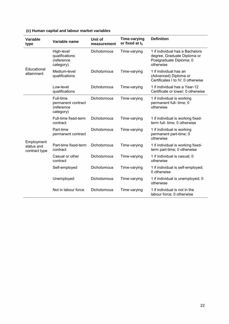
Table 6: List of names and definitions of explanatory variables ................................. 20

Table 7: Discrete time hazard model estimates—escape from first spell of unaffordable housing, 30:40 rule ........................................................................ 26

Table 8: Discrete time hazard model estimates—survival in first spell of affordable housing, 30:40 rule ............................................................................................ 29

Table 9: Un-weighted and weighted frequency of transitions between affordable and unaffordable housing, conditional on previous spell in unaffordable housing ...... 33

Table 10: Odds ratio estimates of relapse from affordable housing back into unaffordable housing (conditional on previous episode of HAS) ......................... 34

Table 11: Odds ratio estimates of rebound back into affordable housing (conditional on previous episode in affordable housing) ........................................................ 36

Table 12: Churning model; coefficient and marginal effect estimates ........................ 39

v

LIST OF FIGURES

Figure 1: Percentage of home owners with a mortgage debt, 1982–2011a .................. 6

Figure 2: Mean LTV of home owners with a mortgage debt, 1990–2011a.................... 6

Figure 3: Mean mortgage debt to income ratio of home owners with a mortgage debt, 1990–2011a .......................................................................................................... 7

vi

ACRONYMS

ABS Australian Bureau of Statistics

AFF Affordable housing

AHURI Australian Housing and Urban Research Institute Limited

CRA Commonwealth Rent Assistance

FaCSIA Australian Government Department of Families, Community Services and Indigenous Affairs

FTB Family Tax Benefit

GFC Global Financial Crisis

HAS Housing Affordability Stress

HCB Housing cost burden ratio

HCR Housing cost ratio

HILDA Housing, Income and Labour Dynamics of Australia Survey

LTV Loan-to-value ratio

SEIFA Socio-Economic Indexes for Areas

1

EXECUTIVE SUMMARY

This is the third report from a research program that investigates the dynamics of housing affordability stress (HAS) in Australia. The first report, by Wood and Ong (2009), tracked the housing affordability trajectories of Australians over the period 2001–06. This first study ended just before the global financial crisis (GFC) and did not capture the impacts of this important economic event on housing affordability in Australia. The second report by Wood et al. (2014) offered more up-to-date descriptive estimates of movements in and out of HAS by exploiting a longer 11-year timeframe that covers 2001–11. Not only does this timeframe allow us to capture the pre- and post-GFC years, the longer period of analysis facilitates analysis of relapse that might result in cycling in and out of HAS.

Our third report extends the descriptive statistical profile offered in the second report by reporting results from numerous regression models that uncover the factors that influence the dynamics of HAS over the period 2001–11. The dataset employed in this report (as well as the previous reports) is the nationally representative Household, Income and Labour Dynamics in Australia (HILDA) Survey. The data’s panel nature allows us to track HAS trajectories over

time. The measurement of housing affordability status largely follows the previous reports. An ‘attribution’ approach is applied, which ensures that while we are tracking individuals, their

housing affordability position is measured on an income unit basis, the latter being the appropriate measurement unit for housing costs. This is because critical variables that affect housing costs (and hence affordability), such as Commonwealth Rent Assistance (CRA) and Family Tax Benefit (FTB), are measured on an income unit basis. Housing costs are defined on a net basis, ensuring that private renters’ rental costs are measured net of CRA and public

renters’ housing costs are rebated rents. Income is defined on an equivalised and after-tax basis. While the previous two reports adopt two definitions of HAS—the 30 per cent rule and the 30:40 rule—we focus on the latter in this report as it is commonly regarded as a more robust measure of HAS than the former. To be specific, in this report we assign a person to HAS when housing costs exceed 30 per cent of household income and income is within the lowest 40 per cent of the household income distribution.

Using HILDA we are able to track the housing affordability profile of 5047 persons over the course of 10 years, from 2001 through to 2011. Of the sample, 1032 persons (20%) are exposed to one or more episodes (waves) of unaffordable housing circumstances (their income places them below the 40th percentile of the income distribution, and they spend more than 30% of their income on housing costs). Exposure to just one episode of HAS is the fate of 579 persons (11.5%) in the sample. However, this still leaves 453 persons with experience of two or more episodes.

Our regression modelling results shed light on the personal characteristics that define ‘dynamic

affordability stress’ subgroups, defined as individuals who:

are especially vulnerable to dropping out of affordable housing and experience difficulty rebounding back into affordable housing

find it difficult to escape HAS, and are inclined to relapse back into HAS if escape is achieved

exhibit episodic housing affordability profiles that feature cycling in and out of HAS.

A key finding is that low-income Australians with dependent children feature prominently in all the three subgroups described above. In particular, those with very young children (aged under five years) and dependent children in their adolescent or young adult years (15–24 years) are particularly prone to falling into these HAS subgroups. One might speculate that housing related cost of living pressures are particularly important because once children reach late teenage years they require separate bedrooms, and infants will similarly add to family size and space demands. Infants will also prompt lower employment participation from (typically) female

2

partners. Low-income migrants from non-English speaking backgrounds also feature strongly within these three HAS subgroups. It might be that these migrants find it more difficult to navigate pathways into sustainable affordable housing due to language difficulties, lack of familiarity with institutional practices in Australian housing markets, or discrimination in housing markets. Unsurprisingly, the unemployed, those not in the labour force and workers on casual job contracts are prone to falling into the dynamic HAS subgroups. Importantly, the self-employed are consistently over-represented in these subgroups as well. This may be attributable to the variable nature of their disposable incomes. We find that variance measures based on self-employed disposable household incomes are roughly twice those in the rest of the workforce.

Our regression models also suggest that the chances of falling into dynamic affordability stress groups are higher in the post-GFC years, after controlling for other factors. Our findings indicate that navigation out of HAS and the ability to sustain affordable housing has become more difficult since the GFC.

The project findings have significant policy implications. The cuts to FTB in the recent 2014 budget will subject those with dependent children to a greater risk of dynamic housing stress due to a freeze in indexation arrangements. Furthermore, because low-income private renters are more likely to be subject to dynamic housing stress than public renters, proposed reform arrangements that introduce market rents for social housing tenants who then become eligible for CRA would likely place social housing tenants at much greater risk of protracted and episodic spells of HAS. Falling rates of outright ownership among older Australians will also result in more persistent and sporadic HAS in later life. This will raise challenges for Australia’s

welfare state given the importance of outright ownership as a traditional pillar supporting retirement incomes policy.

3

1 INTRODUCTION

This is the third in a series of reports that has developed a program of research into the dynamics of housing affordability stress. It began with a study (Wood & Ong 2009) exploring the duration of Australians’ spells in housing affordability stress (HAS). It used the Household, Income and Labour Dynamics in Australia (HILDA) survey to profile the housing affordability trajectories of a nationally representative sample of Australians over the period 2001–06. We were keen to ascertain whether spells in HAS were temporary or enduring and, if temporary, were escapes from HAS permanent? The five-year timeframe was a limitation in two ways. First, it is too short for the analysis of relapse that might punctuate the housing affordability pathways of those evading HAS. Second, the study timeframe ends just as the Global Financial Crisis was about to disrupt the national economy and its housing markets. This shock, and the economic policy response to it, had very significant impacts on interest rates and house prices that are key drivers of the dynamics of housing affordability.

Our new project exploits a longer 11-year timeframe covering the period 2001–11, and employs novel empirical methods to generate additional insights into the dynamics of housing affordability in Australia. The introductory chapter proceeds to sketch in some background material on housing market trends that help explain why housing affordability has become such an important policy issue. It then summarises the key findings from a positioning paper published in November 2014, and describes how this Final Report extends our program of research in new directions, as well as updating findings reported in Wood and Ong (2009).

1.1 Background

Housing affordability has become one of the more important social policy issues because of the widespread belief that housing costs are a growing burden for both private renters and home buyers. Since increasing cost burdens make it more difficult to save when renting, and to meet mortgage payments when purchasing housing, home ownership is increasingly difficult to attain and safeguard. High and rising housing cost burdens therefore pose a threat to Australia’s home ownership society. They also erode living standards, especially those of

private rental households that cannot cross the threshold into owner occupation and do not benefit from that tenure’s asset-welfare attribute (Doling & Elsinga 2013). Finally, those with individual risk factors associated with homelessness (e.g. victims of domestic violence) are arguably more prone to homelessness if supplies of affordable rental housing are scarce (O’Flaherty 2004).

In Wood et al. (2014), we reported various long-run housing market trends that document how changes in the affordability of housing, housing tenure and indebtedness inform these issues. This section extends the timeframe employed in Wood et al. (2014) by two years, a modification made possible by acquisition of the 2011 ABS Survey of Income and Housing. This is helpful because the 2011 survey lengthens the post-GFC era to four years (2007–11), and more firmly identifies whether trends before the crisis have been interrupted or even reversed.1

Table1 below shows how housing in both the main housing tenures has become more unaffordable over the 30-year interval 1982–2011. Back in 1982, the typical private renter devoted 17 per cent of gross household income to meet rent payments. The share of income allotted to rent payments has increased by 6 percentage points since then (to 23%), and the number of households paying more than 30 per cent of gross household income in rent has more than doubled (from 338 000 to 787 000) (see Table 2 below).2 When our study timeframe 1 We have also added two new analyses of long-run trends—measurement of loan to income multiples 1990–2011, and measurement of net housing cost ratio measures 2001–11. 2 Population estimates are generated using households weights made available in each Survey of Income and Housing.

4

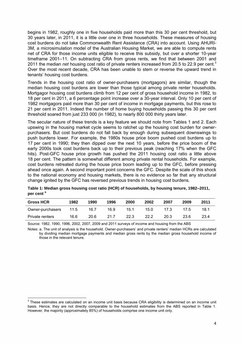
begins in 1982, roughly one in five households paid more than this 30 per cent threshold, but 30 years later, in 2011, it is a little over one in three households. These measures of housing cost burdens do not take Commonwealth Rent Assistance (CRA) into account. Using AHURI-3M, a microsimulation model of the Australian Housing Market, we are able to compute rents net of CRA for those income units eligible to receive this subsidy, but over a shorter 10-year timeframe 2001–11. On subtracting CRA from gross rents, we find that between 2001 and 2011 the median net housing cost ratio of private renters increased from 20.5 to 22.9 per cent.3 Over the most recent decade, CRA has been unable to stem or reverse the upward trend in tenants’ housing cost burdens.

Trends in the housing cost ratio of owner-purchasers (mortgagors) are similar, though the median housing cost burdens are lower than those typical among private renter households. Mortgagor housing cost burdens climb from 12 per cent of gross household income in 1982, to 18 per cent in 2011, a 6 percentage point increase over a 30-year interval. Only 10 per cent of 1982 mortgagors paid more than 30 per cent of income in mortgage payments, but this rose to 21 per cent in 2011. Indeed the number of home buying households passing this 30 per cent threshold soared from just 233 000 (in 1982), to nearly 800 000 thirty years later.

The secular nature of these trends is a key feature we should note from Tables 1 and 2. Each upswing in the housing market cycle seems to ratchet up the housing cost burden for owner-purchasers. But cost burdens do not fall back by enough during subsequent downswings to push burdens lower. For example, the 1980s house price boom pushed cost burdens up to 17 per cent in 1990; they then dipped over the next 10 years, before the price boom of the early 2000s took cost burdens back up to their previous peak (reaching 17% when the GFC hits). Post-GFC house price growth has pushed the 2011 housing cost ratio a little above 18 per cent. The pattern is somewhat different among private rental households. For example, cost burdens retreated during the house price boom leading up to the GFC, before pressing ahead once again. A second important point concerns the GFC. Despite the scale of this shock to the national economy and housing markets, there is no evidence so far that any structural change ignited by the GFC has reversed previous trends in housing cost burdens.

Table 1: Median gross housing cost ratio (HCR) of households, by housing tenure, 1982–2011,

per cent a

Gross HCR 1982 1990 1996 2000 2002 2007 2009 2011

Owner-purchasers 11.5 16.7 16.9 15.1 15.0 17.3 17.5 18.1

Private renters 16.6 20.6 21.7 22.3 22.2 20.3 23.6 23.4

Source: 1982, 1990, 1996, 2002, 2007, 2009 and 2011 surveys of income and housing from the ABS Notes: a. The unit of analysis is the household. Owner-purchasers’ and private renters’ median HCRs are calculated

by dividing median mortgage payments and median gross rents by the median gross household income of those in the relevant tenure.

3 These estimates are calculated on an income unit basis because CRA eligibility is determined on an income unit basis. Hence, they are not directly comparable to the household estimates from the ABS reported in Table 1. However, the majority (approximately 85%) of households comprise one income unit only.

5

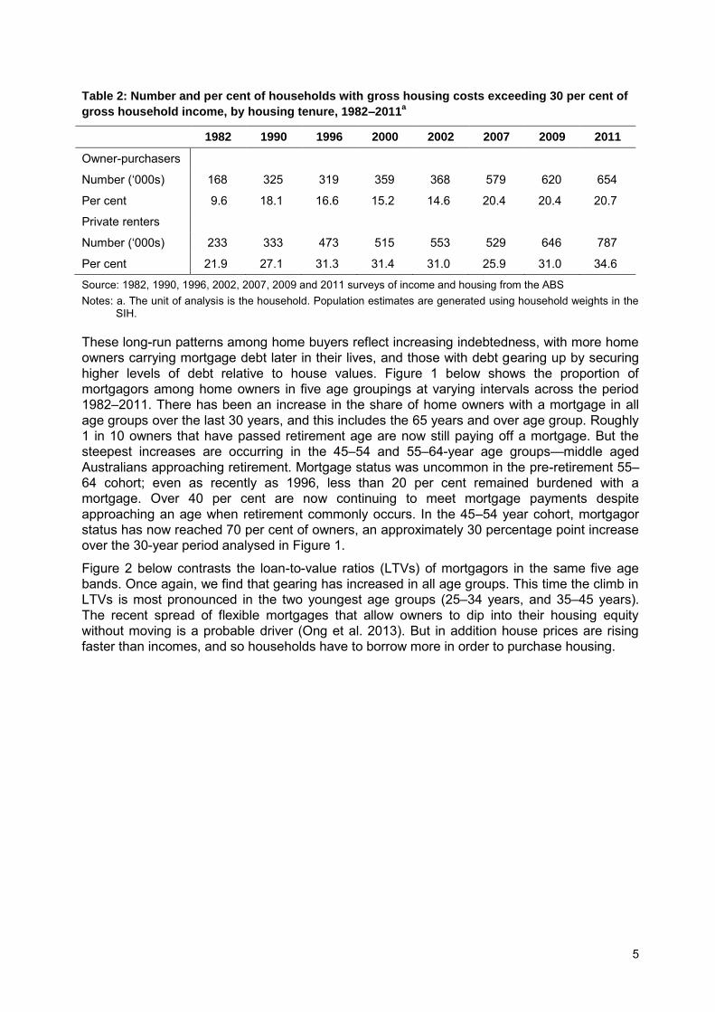
Table 2: Number and per cent of households with gross housing costs exceeding 30 per cent of

gross household income, by housing tenure, 1982–2011a

1982 1990 1996 2000 2002 2007 2009 2011

Owner-purchasers

Number (‘000s) 168 325 319 359 368 579 620 654

Per cent 9.6 18.1 16.6 15.2 14.6 20.4 20.4 20.7

Private renters

Number (‘000s) 233 333 473 515 553 529 646 787

Per cent 21.9 27.1 31.3 31.4 31.0 25.9 31.0 34.6

Source: 1982, 1990, 1996, 2002, 2007, 2009 and 2011 surveys of income and housing from the ABS Notes: a. The unit of analysis is the household. Population estimates are generated using household weights in the

SIH.

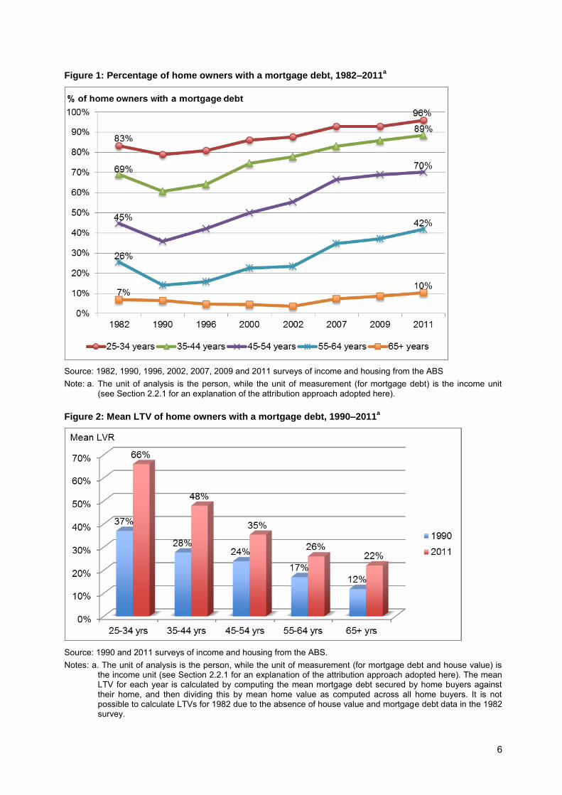
These long-run patterns among home buyers reflect increasing indebtedness, with more home owners carrying mortgage debt later in their lives, and those with debt gearing up by securing higher levels of debt relative to house values. Figure 1 below shows the proportion of mortgagors among home owners in five age groupings at varying intervals across the period 1982–2011. There has been an increase in the share of home owners with a mortgage in all age groups over the last 30 years, and this includes the 65 years and over age group. Roughly 1 in 10 owners that have passed retirement age are now still paying off a mortgage. But the steepest increases are occurring in the 45–54 and 55–64-year age groups—middle aged Australians approaching retirement. Mortgage status was uncommon in the pre-retirement 55–

64 cohort; even as recently as 1996, less than 20 per cent remained burdened with a mortgage. Over 40 per cent are now continuing to meet mortgage payments despite approaching an age when retirement commonly occurs. In the 45–54 year cohort, mortgagor status has now reached 70 per cent of owners, an approximately 30 percentage point increase over the 30-year period analysed in Figure 1.

Figure 2 below contrasts the loan-to-value ratios (LTVs) of mortgagors in the same five age bands. Once again, we find that gearing has increased in all age groups. This time the climb in LTVs is most pronounced in the two youngest age groups (25–34 years, and 35–45 years). The recent spread of flexible mortgages that allow owners to dip into their housing equity without moving is a probable driver (Ong et al. 2013). But in addition house prices are rising faster than incomes, and so households have to borrow more in order to purchase housing.

6

Figure 1: Percentage of home owners with a mortgage debt, 1982–2011a

Source: 1982, 1990, 1996, 2002, 2007, 2009 and 2011 surveys of income and housing from the ABS Note: a. The unit of analysis is the person, while the unit of measurement (for mortgage debt) is the income unit

(see Section 2.2.1 for an explanation of the attribution approach adopted here).

Figure 2: Mean LTV of home owners with a mortgage debt, 1990–2011a

Source: 1990 and 2011 surveys of income and housing from the ABS. Notes: a. The unit of analysis is the person, while the unit of measurement (for mortgage debt and house value) is

the income unit (see Section 2.2.1 for an explanation of the attribution approach adopted here). The mean LTV for each year is calculated by computing the mean mortgage debt secured by home buyers against their home, and then dividing this by mean home value as computed across all home buyers. It is not possible to calculate LTVs for 1982 due to the absence of house value and mortgage debt data in the 1982 survey.

7

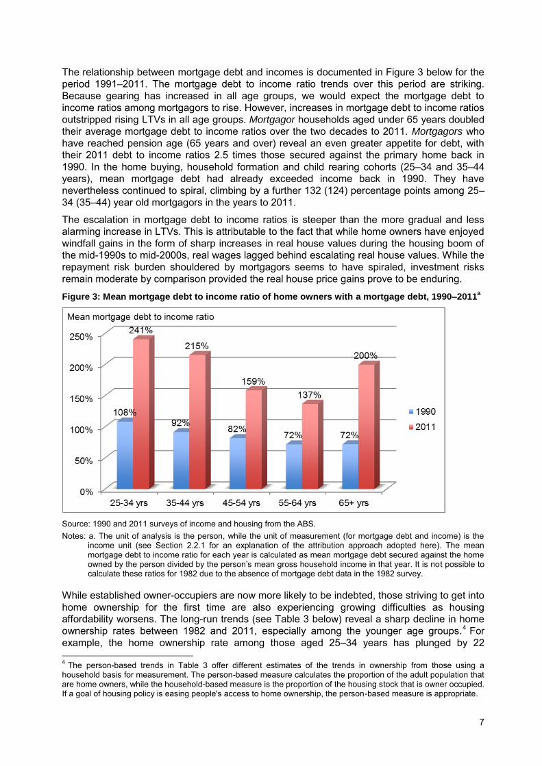
The relationship between mortgage debt and incomes is documented in Figure 3 below for the period 1991–2011. The mortgage debt to income ratio trends over this period are striking. Because gearing has increased in all age groups, we would expect the mortgage debt to income ratios among mortgagors to rise. However, increases in mortgage debt to income ratios outstripped rising LTVs in all age groups. Mortgagor households aged under 65 years doubled their average mortgage debt to income ratios over the two decades to 2011. Mortgagors who have reached pension age (65 years and over) reveal an even greater appetite for debt, with their 2011 debt to income ratios 2.5 times those secured against the primary home back in 1990. In the home buying, household formation and child rearing cohorts (25–34 and 35–44 years), mean mortgage debt had already exceeded income back in 1990. They have nevertheless continued to spiral, climbing by a further 132 (124) percentage points among 25–

34 (35–44) year old mortgagors in the years to 2011.

The escalation in mortgage debt to income ratios is steeper than the more gradual and less alarming increase in LTVs. This is attributable to the fact that while home owners have enjoyed windfall gains in the form of sharp increases in real house values during the housing boom of the mid-1990s to mid-2000s, real wages lagged behind escalating real house values. While the repayment risk burden shouldered by mortgagors seems to have spiraled, investment risks remain moderate by comparison provided the real house price gains prove to be enduring.

Figure 3: Mean mortgage debt to income ratio of home owners with a mortgage debt, 1990–2011a

Source: 1990 and 2011 surveys of income and housing from the ABS. Notes: a. The unit of analysis is the person, while the unit of measurement (for mortgage debt and income) is the

income unit (see Section 2.2.1 for an explanation of the attribution approach adopted here). The mean mortgage debt to income ratio for each year is calculated as mean mortgage debt secured against the home owned by the person divided by the person’s mean gross household income in that year. It is not possible to calculate these ratios for 1982 due to the absence of mortgage debt data in the 1982 survey.

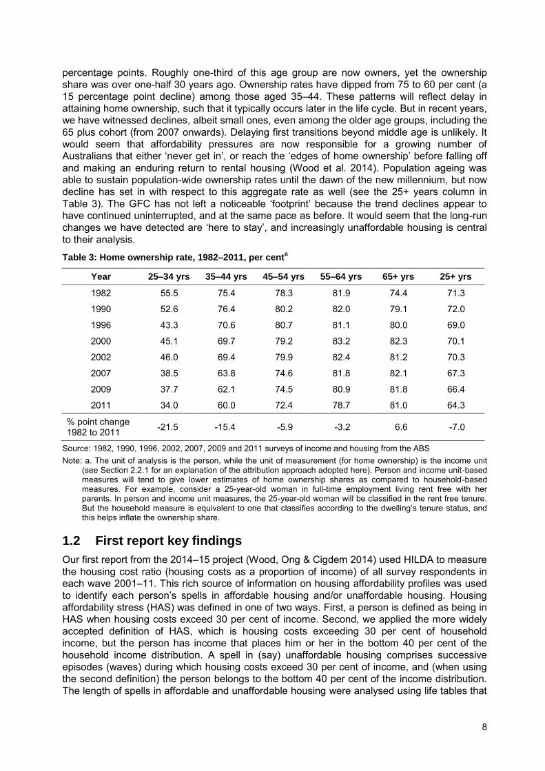
While established owner-occupiers are now more likely to be indebted, those striving to get into home ownership for the first time are also experiencing growing difficulties as housing affordability worsens. The long-run trends (see Table 3 below) reveal a sharp decline in home ownership rates between 1982 and 2011, especially among the younger age groups.4 For example, the home ownership rate among those aged 25–34 years has plunged by 22 4 The person-based trends in Table 3 offer different estimates of the trends in ownership from those using a household basis for measurement. The person-based measure calculates the proportion of the adult population that are home owners, while the household-based measure is the proportion of the housing stock that is owner occupied. If a goal of housing policy is easing people's access to home ownership, the person-based measure is appropriate.

8

percentage points. Roughly one-third of this age group are now owners, yet the ownership share was over one-half 30 years ago. Ownership rates have dipped from 75 to 60 per cent (a 15 percentage point decline) among those aged 35–44. These patterns will reflect delay in attaining home ownership, such that it typically occurs later in the life cycle. But in recent years, we have witnessed declines, albeit small ones, even among the older age groups, including the 65 plus cohort (from 2007 onwards). Delaying first transitions beyond middle age is unlikely. It would seem that affordability pressures are now responsible for a growing number of Australians that either ‘never get in’, or reach the ‘edges of home ownership’ before falling off

and making an enduring return to rental housing (Wood et al. 2014). Population ageing was able to sustain population-wide ownership rates until the dawn of the new millennium, but now decline has set in with respect to this aggregate rate as well (see the 25+ years column in Table 3). The GFC has not left a noticeable ‘footprint’ because the trend declines appear to

have continued uninterrupted, and at the same pace as before. It would seem that the long-run changes we have detected are ‘here to stay’, and increasingly unaffordable housing is central

to their analysis.

Table 3: Home ownership rate, 1982–2011, per centa

Year 25–34 yrs 35–44 yrs 45–54 yrs 55–64 yrs 65+ yrs 25+ yrs

1982 55.5 75.4 78.3 81.9 74.4 71.3

1990 52.6 76.4 80.2 82.0 79.1 72.0

1996 43.3 70.6 80.7 81.1 80.0 69.0

2000 45.1 69.7 79.2 83.2 82.3 70.1

2002 46.0 69.4 79.9 82.4 81.2 70.3

2007 38.5 63.8 74.6 81.8 82.1 67.3

2009 37.7 62.1 74.5 80.9 81.8 66.4

2011 34.0 60.0 72.4 78.7 81.0 64.3

% point change 1982 to 2011 -21.5 -15.4 -5.9 -3.2 6.6 -7.0

Source: 1982, 1990, 1996, 2002, 2007, 2009 and 2011 surveys of income and housing from the ABS Note: a. The unit of analysis is the person, while the unit of measurement (for home ownership) is the income unit

(see Section 2.2.1 for an explanation of the attribution approach adopted here). Person and income unit-based measures will tend to give lower estimates of home ownership shares as compared to household-based measures. For example, consider a 25-year-old woman in full-time employment living rent free with her parents. In person and income unit measures, the 25-year-old woman will be classified in the rent free tenure. But the household measure is equivalent to one that classifies according to the dwelling’s tenure status, and this helps inflate the ownership share.

1.2 First report key findings

Our first report from the 2014–15 project (Wood, Ong & Cigdem 2014) used HILDA to measure the housing cost ratio (housing costs as a proportion of income) of all survey respondents in each wave 2001–11. This rich source of information on housing affordability profiles was used to identify each person’s spells in affordable housing and/or unaffordable housing. Housing

affordability stress (HAS) was defined in one of two ways. First, a person is defined as being in HAS when housing costs exceed 30 per cent of income. Second, we applied the more widely accepted definition of HAS, which is housing costs exceeding 30 per cent of household income, but the person has income that places him or her in the bottom 40 per cent of the household income distribution. A spell in (say) unaffordable housing comprises successive episodes (waves) during which housing costs exceed 30 per cent of income, and (when using the second definition) the person belongs to the bottom 40 per cent of the income distribution. The length of spells in affordable and unaffordable housing were analysed using life tables that

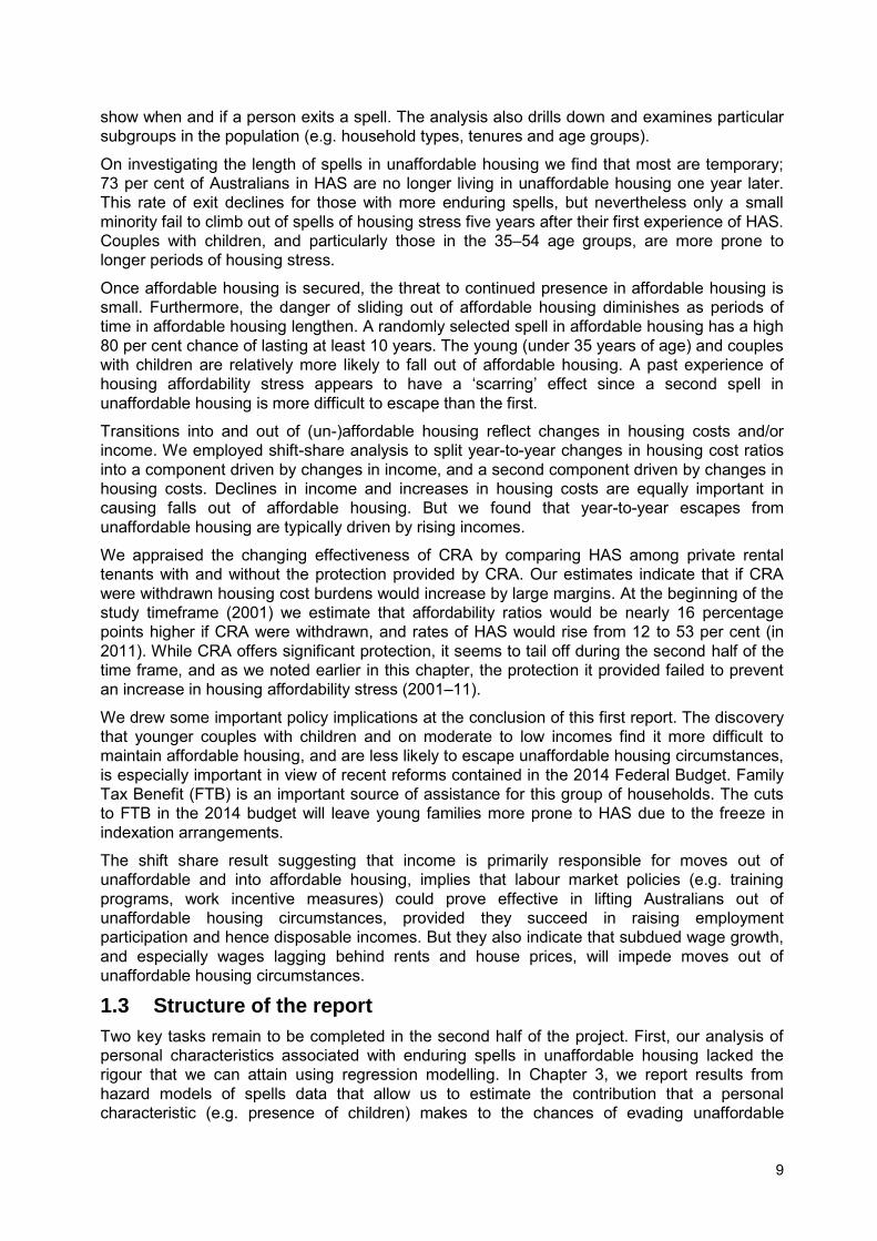
9

show when and if a person exits a spell. The analysis also drills down and examines particular subgroups in the population (e.g. household types, tenures and age groups).

On investigating the length of spells in unaffordable housing we find that most are temporary; 73 per cent of Australians in HAS are no longer living in unaffordable housing one year later. This rate of exit declines for those with more enduring spells, but nevertheless only a small minority fail to climb out of spells of housing stress five years after their first experience of HAS. Couples with children, and particularly those in the 35–54 age groups, are more prone to longer periods of housing stress.

Once affordable housing is secured, the threat to continued presence in affordable housing is small. Furthermore, the danger of sliding out of affordable housing diminishes as periods of time in affordable housing lengthen. A randomly selected spell in affordable housing has a high 80 per cent chance of lasting at least 10 years. The young (under 35 years of age) and couples with children are relatively more likely to fall out of affordable housing. A past experience of housing affordability stress appears to have a ‘scarring’ effect since a second spell in

unaffordable housing is more difficult to escape than the first.

Transitions into and out of (un-)affordable housing reflect changes in housing costs and/or income. We employed shift-share analysis to split year-to-year changes in housing cost ratios into a component driven by changes in income, and a second component driven by changes in housing costs. Declines in income and increases in housing costs are equally important in causing falls out of affordable housing. But we found that year-to-year escapes from unaffordable housing are typically driven by rising incomes.

We appraised the changing effectiveness of CRA by comparing HAS among private rental tenants with and without the protection provided by CRA. Our estimates indicate that if CRA were withdrawn housing cost burdens would increase by large margins. At the beginning of the study timeframe (2001) we estimate that affordability ratios would be nearly 16 percentage points higher if CRA were withdrawn, and rates of HAS would rise from 12 to 53 per cent (in 2011). While CRA offers significant protection, it seems to tail off during the second half of the time frame, and as we noted earlier in this chapter, the protection it provided failed to prevent an increase in housing affordability stress (2001–11).

We drew some important policy implications at the conclusion of this first report. The discovery that younger couples with children and on moderate to low incomes find it more difficult to maintain affordable housing, and are less likely to escape unaffordable housing circumstances, is especially important in view of recent reforms contained in the 2014 Federal Budget. Family Tax Benefit (FTB) is an important source of assistance for this group of households. The cuts to FTB in the 2014 budget will leave young families more prone to HAS due to the freeze in indexation arrangements.

The shift share result suggesting that income is primarily responsible for moves out of unaffordable and into affordable housing, implies that labour market policies (e.g. training programs, work incentive measures) could prove effective in lifting Australians out of unaffordable housing circumstances, provided they succeed in raising employment participation and hence disposable incomes. But they also indicate that subdued wage growth, and especially wages lagging behind rents and house prices, will impede moves out of unaffordable housing circumstances.

1.3 Structure of the report

Two key tasks remain to be completed in the second half of the project. First, our analysis of personal characteristics associated with enduring spells in unaffordable housing lacked the rigour that we can attain using regression modelling. In Chapter 3, we report results from hazard models of spells data that allow us to estimate the contribution that a personal characteristic (e.g. presence of children) makes to the chances of evading unaffordable

10

housing, after controlling for other relevant factors. Although the HILDA sample of Australians quickly escapes unaffordable housing circumstances, our first report did reveal evidence of a reversion back into HAS at a later date. A second task is the subject of Chapter 4, where we use regression models to identify the personal characteristics distinguishing people cycling back and forth between unaffordable and affordable housing. A description of methods is sandwiched between the current chapter and the two results chapters; a final chapter sums up by identifying key discoveries, their implications, and the gaps in our knowledge that future research could fill.

11

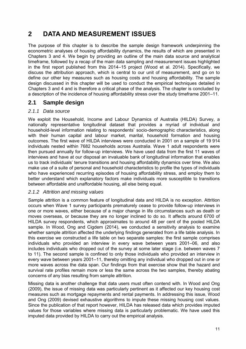
2 DATA AND MEASUREMENT ISSUES

The purpose of this chapter is to describe the sample design framework underpinning the econometric analyses of housing affordability dynamics, the results of which are presented in Chapters 3 and 4. We begin by providing an outline of the main data source and analytical timeframe, followed by a recap of the main data sampling and measurement issues highlighted in the first report published from this 2014–15 project (Wood et al. 2014). Specifically, we discuss the attribution approach, which is central to our unit of measurement, and go on to define our other key measures such as housing costs and housing affordability. The sample design discussed in this chapter will be used to conduct the empirical techniques detailed in Chapters 3 and 4 and is therefore a critical phase of the analysis. The chapter is concluded by a description of the incidence of housing affordability stress over the study timeframe 2001–11.

2.1 Sample design

2.1.1 Data source

We exploit the Household, Income and Labour Dynamics of Australia (HILDA) Survey, a nationally representative longitudinal dataset that provides a myriad of individual and household-level information relating to respondents’ socio-demographic characteristics, along with their human capital and labour market, marital, household formation and housing outcomes. The first wave of HILDA interviews were conducted in 2001 on a sample of 19 914 individuals nested within 7682 households across Australia. Wave 1 adult respondents were then pursued annually for follow-up interviews. We have used data from the first 11 waves of interviews and have at our disposal an invaluable bank of longitudinal information that enables us to track individuals’ tenure transitions and housing affordability dynamics over time. We also

make use of a suite of personal and household characteristics to profile the types of individuals who have experienced recurring episodes of housing affordability stress, and employ them to better understand which explanatory factors make individuals more susceptible to transitions between affordable and unaffordable housing, all else being equal.

2.1.2 Attrition and missing values

Sample attrition is a common feature of longitudinal data and HILDA is no exception. Attrition occurs when Wave 1 survey participants prematurely cease to provide follow-up interviews in one or more waves, either because of a major change in life circumstances such as death or moves overseas, or because they are no longer inclined to do so. It affects around 6700 of HILDA survey respondents, which approximates to around 48 per cent of the pooled HILDA sample. In Wood, Ong and Cigdem (2014), we conducted a sensitivity analysis to examine whether sample attrition affected the underlying findings generated from a life table analysis. In this exercise we constructed a life table on two separate samples: the first sample comprises individuals who provided an interview in every wave between years 2001–06, and also includes individuals who dropped out of the survey at some later stage (i.e. between waves 7 to 11). The second sample is confined to only those individuals who provided an interview in every wave between years 2001–11, thereby omitting any individual who dropped out in one or more waves across the data span. Our findings from that exercise show that the hazard and survival rate profiles remain more or less the same across the two samples, thereby abating concerns of any bias resulting from sample attrition.

Missing data is another challenge that data users must often contend with. In Wood and Ong (2009), the issue of missing data was particularly pertinent as it affected our key housing cost measures such as mortgage repayments and rental payments. In addressing this issue, Wood and Ong (2009) devised exhaustive algorithms to impute these missing housing cost values. Since the publication of that report however, HILDA has released data which provides imputed values for those variables where missing data is particularly problematic. We have used this imputed data provided by HILDA to carry out the empirical analysis.

12

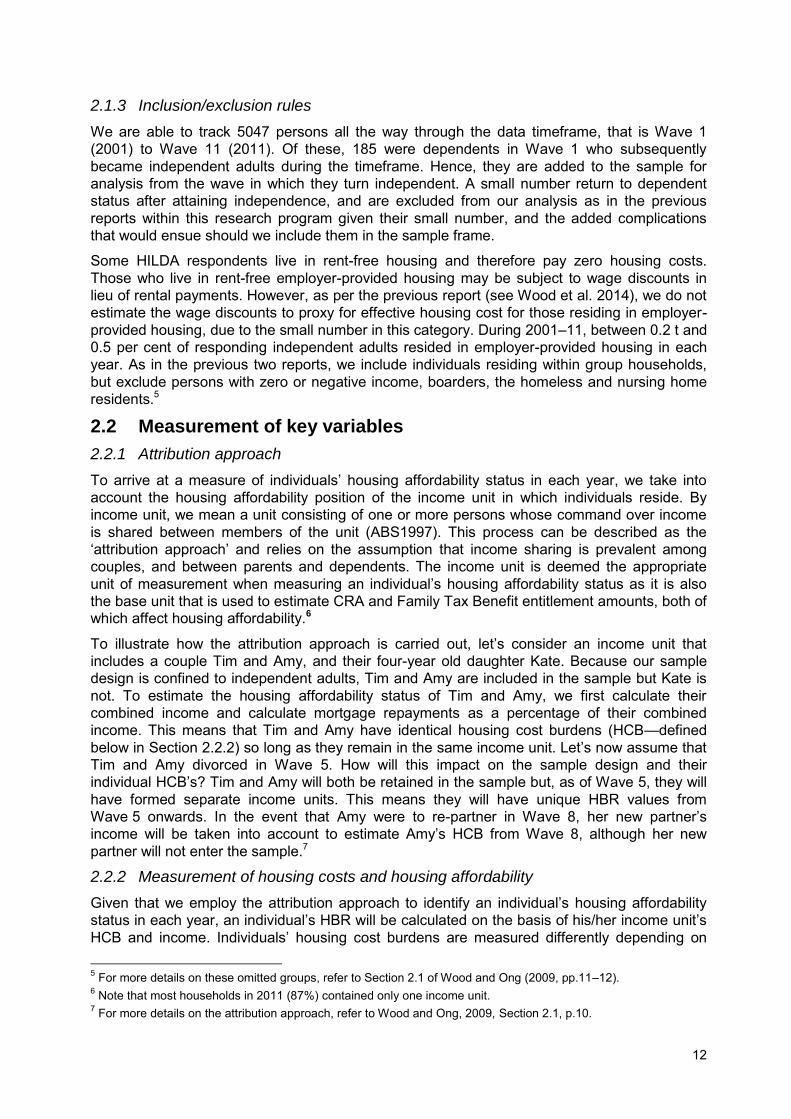
2.1.3 Inclusion/exclusion rules

We are able to track 5047 persons all the way through the data timeframe, that is Wave 1 (2001) to Wave 11 (2011). Of these, 185 were dependents in Wave 1 who subsequently became independent adults during the timeframe. Hence, they are added to the sample for analysis from the wave in which they turn independent. A small number return to dependent status after attaining independence, and are excluded from our analysis as in the previous reports within this research program given their small number, and the added complications that would ensue should we include them in the sample frame.

Some HILDA respondents live in rent-free housing and therefore pay zero housing costs. Those who live in rent-free employer-provided housing may be subject to wage discounts in lieu of rental payments. However, as per the previous report (see Wood et al. 2014), we do not estimate the wage discounts to proxy for effective housing cost for those residing in employer-provided housing, due to the small number in this category. During 2001–11, between 0.2 t and 0.5 per cent of responding independent adults resided in employer-provided housing in each year. As in the previous two reports, we include individuals residing within group households, but exclude persons with zero or negative income, boarders, the homeless and nursing home residents.5

2.2 Measurement of key variables

2.2.1 Attribution approach

To arrive at a measure of individuals’ housing affordability status in each year, we take into

account the housing affordability position of the income unit in which individuals reside. By income unit, we mean a unit consisting of one or more persons whose command over income is shared between members of the unit (ABS1997). This process can be described as the ‘attribution approach’ and relies on the assumption that income sharing is prevalent among couples, and between parents and dependents. The income unit is deemed the appropriate unit of measurement when measuring an individual’s housing affordability status as it is also

the base unit that is used to estimate CRA and Family Tax Benefit entitlement amounts, both of which affect housing affordability.6

To illustrate how the attribution approach is carried out, let’s consider an income unit that

includes a couple Tim and Amy, and their four-year old daughter Kate. Because our sample design is confined to independent adults, Tim and Amy are included in the sample but Kate is not. To estimate the housing affordability status of Tim and Amy, we first calculate their combined income and calculate mortgage repayments as a percentage of their combined income. This means that Tim and Amy have identical housing cost burdens (HCB—defined below in Section 2.2.2) so long as they remain in the same income unit. Let’s now assume that

Tim and Amy divorced in Wave 5. How will this impact on the sample design and their individual HCB’s? Tim and Amy will both be retained in the sample but, as of Wave 5, they will have formed separate income units. This means they will have unique HBR values from Wave 5 onwards. In the event that Amy were to re-partner in Wave 8, her new partner’s

income will be taken into account to estimate Amy’s HCB from Wave 8, although her new partner will not enter the sample.7

2.2.2 Measurement of housing costs and housing affordability

Given that we employ the attribution approach to identify an individual’s housing affordability

status in each year, an individual’s HBR will be calculated on the basis of his/her income unit’s

HCB and income. Individuals’ housing cost burdens are measured differently depending on

5 For more details on these omitted groups, refer to Section 2.1 of Wood and Ong (2009, pp.11–12). 6 Note that most households in 2011 (87%) contained only one income unit. 7 For more details on the attribution approach, refer to Wood and Ong, 2009, Section 2.1, p.10.

13

their income unit’s tenure status. For owner-purchasers, housing cost burdens are estimated on the basis of their mortgage repayments. This means that outright owners have zero housing costs given that they have no mortgage. This is also the case for individuals living in rent-free accommodation. For private renters, housing costs are measured as rent minus CRA while for public renters it is their reported rebated rents. A person’s income is measured in terms of the

income unit’s disposable income. This has to be equivalised in order to adjust the reported disposable income measure for income unit size. Hence, we assign the greatest weight to the first and second adult members (1 and 0.7, respectively), and the least weight on dependent children (weight of 0.5 for each additional child).8

As mentioned above, the HBR is estimated on an income unit basis and is calculated as the ratio of net housing costs to equivalised disposable income. For private renters in receipt of CRA, HCB is estimated by subtracting CRA from housing costs as opposed to treating it like residual income and adding to income; the rationale for doing it this way is that CRA entitlements are dependent on the amount of fortnightly rent paid to a private landlord, and should therefore be thought of as a price subsidy rather than an income transfer. We employ the microsimulation model AHURI-3M to compute CRA eligibility and entitlements. Benchmarked on HILDA data, AHURI-3M takes into account individuals’ socio-demographic characteristics as reported in each year over the period 2001–11, including their income unit type, number of dependents, amount of rent paid and household income. The computation of CRA entitlements also factors in the income support received from other types of government program.9

Housing Affordability Stress (HAS) is defined in terms of the widely-used 30/40 rule. In accordance with this rule, an individual is regarded as being in HAS when their housing costs exceed 30 per cent of their income unit’s equivalised disposable income and their income leaves them in the bottom 40 per cent of the household income distribution. The 30/40 rule has its critics. However research reported in Rowley, Ong and Haffner (2014) shows that the 30:40 rule is a better indicator of housing-related financial stress if it is applied within a longitudinal context where the duration of spells in HAS is the focus. A more detailed discussion of the issues is presented in Wood, Ong and Cigdem (2014).

2.2.3 Descriptives

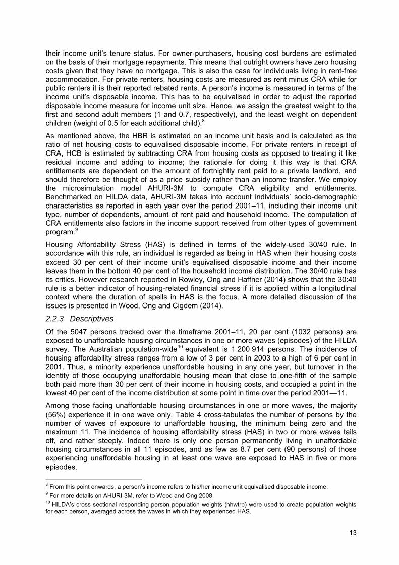
Of the 5047 persons tracked over the timeframe 2001–11, 20 per cent (1032 persons) are exposed to unaffordable housing circumstances in one or more waves (episodes) of the HILDA survey. The Australian population-wide10 equivalent is 1 200 914 persons. The incidence of housing affordability stress ranges from a low of 3 per cent in 2003 to a high of 6 per cent in 2001. Thus, a minority experience unaffordable housing in any one year, but turnover in the identity of those occupying unaffordable housing mean that close to one-fifth of the sample both paid more than 30 per cent of their income in housing costs, and occupied a point in the lowest 40 per cent of the income distribution at some point in time over the period 2001—11.

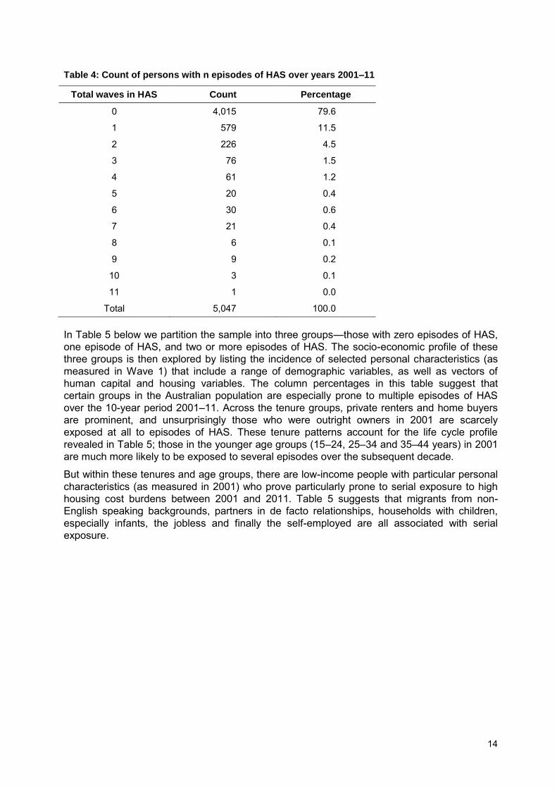
Among those facing unaffordable housing circumstances in one or more waves, the majority (56%) experience it in one wave only. Table 4 cross-tabulates the number of persons by the number of waves of exposure to unaffordable housing, the minimum being zero and the maximum 11. The incidence of housing affordability stress (HAS) in two or more waves tails off, and rather steeply. Indeed there is only one person permanently living in unaffordable housing circumstances in all 11 episodes, and as few as 8.7 per cent (90 persons) of those experiencing unaffordable housing in at least one wave are exposed to HAS in five or more episodes. 8 From this point onwards, a person’s income refers to his/her income unit equivalised disposable income. 9 For more details on AHURI-3M, refer to Wood and Ong 2008. 10 HILDA’s cross sectional responding person population weights (hhwtrp) were used to create population weights for each person, averaged across the waves in which they experienced HAS.

14

Table 4: Count of persons with n episodes of HAS over years 2001–11

Total waves in HAS Count Percentage

0 4,015 79.6

1 579 11.5

2 226 4.5

3 76 1.5

4 61 1.2

5 20 0.4

6 30 0.6

7 21 0.4

8 6 0.1

9 9 0.2

10 3 0.1

11 1 0.0

Total 5,047 100.0

In Table 5 below we partition the sample into three groups—those with zero episodes of HAS, one episode of HAS, and two or more episodes of HAS. The socio-economic profile of these three groups is then explored by listing the incidence of selected personal characteristics (as measured in Wave 1) that include a range of demographic variables, as well as vectors of human capital and housing variables. The column percentages in this table suggest that certain groups in the Australian population are especially prone to multiple episodes of HAS over the 10-year period 2001–11. Across the tenure groups, private renters and home buyers are prominent, and unsurprisingly those who were outright owners in 2001 are scarcely exposed at all to episodes of HAS. These tenure patterns account for the life cycle profile revealed in Table 5; those in the younger age groups (15–24, 25–34 and 35–44 years) in 2001 are much more likely to be exposed to several episodes over the subsequent decade.

But within these tenures and age groups, there are low-income people with particular personal characteristics (as measured in 2001) who prove particularly prone to serial exposure to high housing cost burdens between 2001 and 2011. Table 5 suggests that migrants from non-English speaking backgrounds, partners in de facto relationships, households with children, especially infants, the jobless and finally the self-employed are all associated with serial exposure.

15

Table 5: Housing, locational, demographic and labour market characteristics in Wave 1 (year

2001) of individuals by total number of episodes in HAS between 2001–11

No. of episodes in HAS 0 1 2 or more

Count % Count % Count %

Outright owner 1,564 38.95 56 9.67 20 4.42 Owner-purchaser 1,483 36.94 294 50.78 249 54.97 Private renter 683 17.01 175 30.22 151 33.33 Public renter 122 3.04 33 5.7 20 4.42 Rent free 163 4.06 21 3.63 13 2.87

Lives in inner city 2,456 61.17 381 65.8 275 60.71 Lives in inner regional 994 24.76 138 23.83 125 27.59 Lives in outer regional 565 14.07 60 10.36 53 11.7

Aged 15–24 186 4.63 67 11.57 9.93 9.93 Aged 25–34 677 16.86 186 32.12 146 32.23 Aged 35–44 1,010 25.16 174 30.05 158 34.88 Aged 45–54 926 23.06 82 14.16 74 16.34 Aged 55 and over 1,216 30.29 70 12.09 30 6.62 Born in overseas English-speaking country 491 12.23 67 11.57 42 9.27 Born in overseas non-English-speaking country 410 10.21 82 14.16 86 18.98 Indigenous Australian 53 1.32 4 0.69 3 0.66 Non-indigenous Australian 3,061 76.24 426 73.58 322 71.08 Bad health 864 21.52 100 17.27 87 19.21

Married 2,567 64.03 351 60.62 300 66.23 De facto 374 9.33 89 15.37 63 13.91 Divorced 116 2.89 20 3.45 19 4.19 Separated 268 6.68 29 5.01 13 2.87 Widowed 194 4.84 9 1.55 6 1.32 Single 490 12.22 81 13.99 52 11.48 At least one child aged 0–4 yrs 538 13.4 157 27.12 189 41.72 At least one child aged 5–9 yrs 567 14.12 161 27.81 137 30.24 At least one child aged 10–14 yrs 597 15 121 20.9 104 22.96 At least one child aged 15–24 yrs 388 9.66 60 10.36 47 10.38 High-level qualifications 924 23.02 126 21.76 76 16.78 Medium-level qualifications 1,148 28.6 190 32.82 136 30.02 Low-level qualifications 1,942 48.38 263 45.42 241 53.2

Full-time, permanent contract 1,380 34.37 186 32.12 94 20.75 Full-time, fixed term contract 156 3.89 22 3.8 16 3.53 Part-time, permanent contract 290 7.22 39 6.74 24 5.3 Part-time, fixed term contract 48 1.2 5 0.86 4 0.88 Casual contract 398 9.91 76 13.13 49 10.82 Unemployed 85 2.12 25 4.32 36 7.95 NILF 1,243 30.96 152 26.25 139 30.68 Self-employed 405 10.09 71 12.26 89 19.65 Total count of persons 4,015 579 453

16

3 ARE SPELLS IN (UN-)AFFORDABLE HOUSING ENDURING? MODELLING RESULTS

3.1 Introduction

In this chapter we model the factors influencing a person’s chances of escaping unaffordable

housing stress, and those shaping the chances of survival in affordable housing. It extends the descriptive analysis in Wood et al. (2014) by using regression modelling techniques to more rigorously identify key variables driving transitions across the boundaries separating affordable and unaffordable housing. It also builds on the modelling work reported in Wood and Ong (2009) which analysed these transitions in the short 2001–06 period preceding the turbulence ignited by the Global Financial Crisis (GFC). This research project extends the study timeframe to the longer period 2001–11.

We use standard techniques for modelling the occurrence and timing of events, where events are represented by a transition from one status to another. These techniques have a wide range of applications in medical research fields as well as the social sciences. They include subjects such as survival following major surgery, recidivism among ex-prisoners and the length of spells on welfare program. The length of time spent in a status is commonly referred to as a spell, and events marking interruption to spells are the transitions the researcher is aiming to analyse. Each spell is broken up into a series of episodes (or waves) of equal length.

In this research project we analyse one-year episodes, and the events are transitions into (un-)affordable housing. The start of a spell is the first year that the individual is recorded as occupying (un-)affordable housing. 11 Statistical modelling of transitions from one status to another are typically referred to as hazard or survival models, reflecting their origins in medical research. Acquiring and sustaining (un-)affordable housing over a period of time is then described as survival, while falling out of (un-)affordable housing is the hazard.12 The duration of spells in affordable and unaffordable housing are separately analysed.

Analysis of spells data poses statistical challenges. To appreciate these challenges note that with longitudinal data we are able to calculate how many waves a person remains in (un-)affordable housing. We could simply cross-tabulate the average length of these spells with personal characteristics and thereby uncover the relationships that we are interested in identifying. Multivariate analysis could also be conducted by regressing the length of each person’s spell in (un-)affordable housing on variables that are expected to influence the duration of spells. Unfortunately this standard approach is flawed; some spells used in the statistical analysis are completed, but others are ongoing (censored) at the end of the data collection exercise, but the standard approach we have described treats all spells as if they were concluded, and a transition to a different state (affordable or unaffordable housing) has been completed. An alternative hazard (or survival) modelling approach is required that addresses the problems raised by censored data.

Central to this approach is the estimation of logit models to uncover the relationship between the conditional probability13 of escaping housing affordability stress and a range of explanatory variables, as well as that between the conditional probability of falling out of affordable housing and these same explanatory variables. The explanatory variables can take two forms, time 11 The reliance on one-year episodes is subject to the limitation that any (un-)affordable housing spells of less than a year will not be captured if they occur between the annual interviews of respondents. Hence, the number of spells will likely be under-estimated. 12 This is statistical convention that does not necessarily conform to lay use of the words. For example, survival in a spell of unaffordable housing makes less sense in common parlance. 13 The probability of transitioning from status x to another status y in episode t having survived in status x through to t-1, where t=1,2,3….n is the index representing episodes. The conditional probability is often referred to as the hazard rate.

17

indicators and predictors. Time indicators index the episodes (discrete time periods) that comprise a spell of (un-) affordable housing. If the maximum possible duration of a spell is n years, there are n indicators 𝐷𝑡 𝑤ℎ𝑒𝑟𝑒 𝑡 = 1,2,3 … . 𝑛 𝑎𝑛𝑑 𝐷𝑡 = 1 if the spell is ongoing in the time interval t, zero otherwise. The coefficient estimates (�̂�𝑡) generated by these indicators can be transformed in order to describe how the conditional probabilities evolve as an experience in (un-)affordable housing unfolds. This array of conditional probabilities is commonly referred to as the baseline hazard. When predictor variables are omitted from the logit model, the �̂�𝑡 represent the hazard rates in the life tables reported in Wood et al. (2014, Tables 7 and 8). On including predictor variables the baseline hazard is described for the reference group and defined when setting all the predictor variables to zero. Thus any change to the model specification that adds or subtracts predictor variables changes the definition of the reference group that the baseline hazard profiles.

Predictor variables are measures that a priori reasoning suggests as factors that should be influential in shaping the chances of exiting periods of (un-)affordable housing. Once again the coefficient estimates ( �̂�𝑘 ) can be transformed to obtain the increments in hazard rates (conditional probabilities), controlling for the other predictors in the model. The �̂�𝑘 are more frequently converted into odds ratios that are more intuitively appealing. When the predictor variable is a dummy variable—for example, a variable such as divorced that indicates whether the individual was a divorcee in any Year t of a spell—the odds ratio is the odds of event occurrence when a person is a divorcee, relative to the odds of event occurrence when a person is married (the reference category).14 The odds ratio is then a measure of how likely divorcees are to escape from (say) housing affordability stress, relative to marrieds. If the odds ratio is one-half, divorcees are half as likely (compared to marrieds) to evade unaffordable housing in episode t, given persistent housing affordability stress through to t-1. Odds ratio estimates are presented in the findings section below.

3.2 Data and model specification

We have designed a person-period data set for the purposes of estimating hazard models. This data set has been described in Chapter 2. Here we focus on one feature of this data set—censoring—as the assumptions we make about censoring are important to the reliability of model estimates. To illustrate the concept suppose that our task is to identify and measure the influence of variables determining the chances of tumbling out of affordable housing. The data set will then comprise people that have experienced one or more spells in affordable housing, and those persons will have a separate record for each episode during which he/she continues to reside in affordable housing. There are then two types of cases; the first are those unable to maintain affordable housing through to the end of the data collection period–2011. For example, consider a low-income individual who is first recorded as living in affordable housing in Wave 6 (2006) of the HILDA Survey. Imagine that the individual continues in affordable housing until Wave 9 (2009) when a sharp rise in housing costs pushes him or her into housing affordability stress, given a continuation of low-income status. We label the Wave 6 observation as corresponding to Year 0 of an affordable housing spell; interviewees are asked about housing and other circumstances once a year, so the first time we record whether a transition has been made will be Wave 7 that is then labelled Year 1 of the affordable housing spell (the spell has by Wave 7 lasted one year). The individual is at risk of falling out of affordable housing from Wave 7, or Year 1 onwards. In Wave 9 corresponding to what would be Year 3 of this spell, the individual falls out of affordable housing. In the person-period data

14 The odds of an event occurring are given by:

𝑝𝑟𝑜𝑏𝑎𝑏𝑖𝑙𝑖𝑡𝑦1 − 𝑝𝑟𝑜𝑏𝑎𝑏𝑖𝑙𝑖𝑡𝑦⁄

In hazard analyses, the quotient contains conditional probabilities. If the conditional probability is 0.8, for example, the odds of event occurrence are 4, which means that the event is four times more likely to occur in t than not to occur.

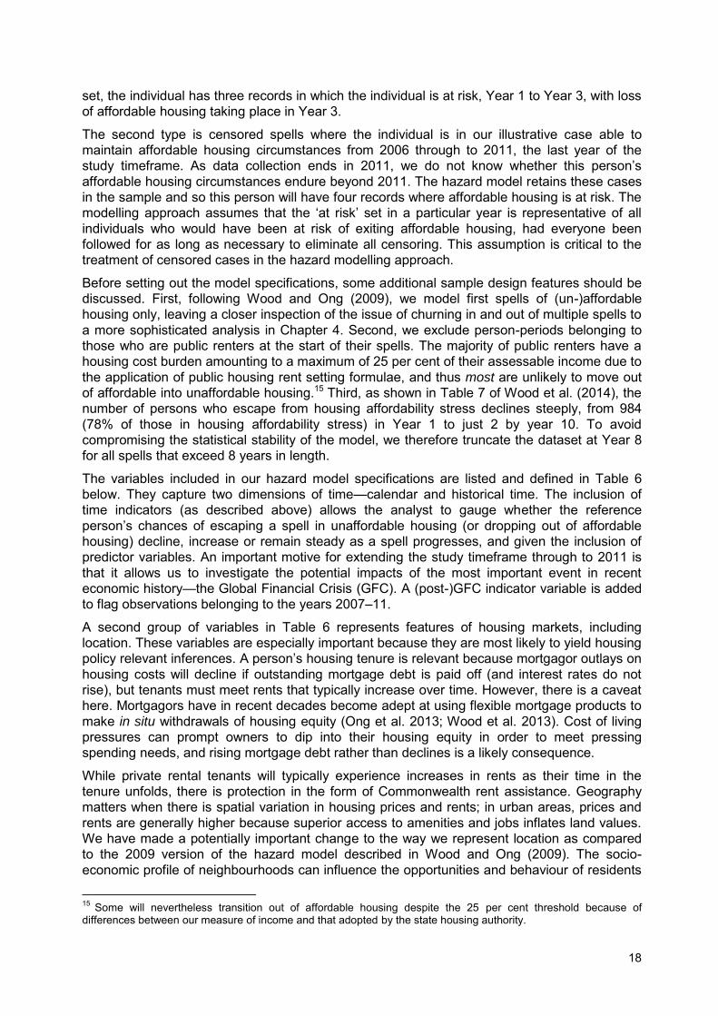
18

set, the individual has three records in which the individual is at risk, Year 1 to Year 3, with loss of affordable housing taking place in Year 3.

The second type is censored spells where the individual is in our illustrative case able to maintain affordable housing circumstances from 2006 through to 2011, the last year of the study timeframe. As data collection ends in 2011, we do not know whether this person’s

affordable housing circumstances endure beyond 2011. The hazard model retains these cases in the sample and so this person will have four records where affordable housing is at risk. The modelling approach assumes that the ‘at risk’ set in a particular year is representative of all

individuals who would have been at risk of exiting affordable housing, had everyone been followed for as long as necessary to eliminate all censoring. This assumption is critical to the treatment of censored cases in the hazard modelling approach.

Before setting out the model specifications, some additional sample design features should be discussed. First, following Wood and Ong (2009), we model first spells of (un-)affordable housing only, leaving a closer inspection of the issue of churning in and out of multiple spells to a more sophisticated analysis in Chapter 4. Second, we exclude person-periods belonging to those who are public renters at the start of their spells. The majority of public renters have a housing cost burden amounting to a maximum of 25 per cent of their assessable income due to the application of public housing rent setting formulae, and thus most are unlikely to move out of affordable into unaffordable housing.15 Third, as shown in Table 7 of Wood et al. (2014), the number of persons who escape from housing affordability stress declines steeply, from 984 (78% of those in housing affordability stress) in Year 1 to just 2 by year 10. To avoid compromising the statistical stability of the model, we therefore truncate the dataset at Year 8 for all spells that exceed 8 years in length.

The variables included in our hazard model specifications are listed and defined in Table 6 below. They capture two dimensions of time—calendar and historical time. The inclusion of time indicators (as described above) allows the analyst to gauge whether the reference person’s chances of escaping a spell in unaffordable housing (or dropping out of affordable

housing) decline, increase or remain steady as a spell progresses, and given the inclusion of predictor variables. An important motive for extending the study timeframe through to 2011 is that it allows us to investigate the potential impacts of the most important event in recent economic history—the Global Financial Crisis (GFC). A (post-)GFC indicator variable is added to flag observations belonging to the years 2007–11.

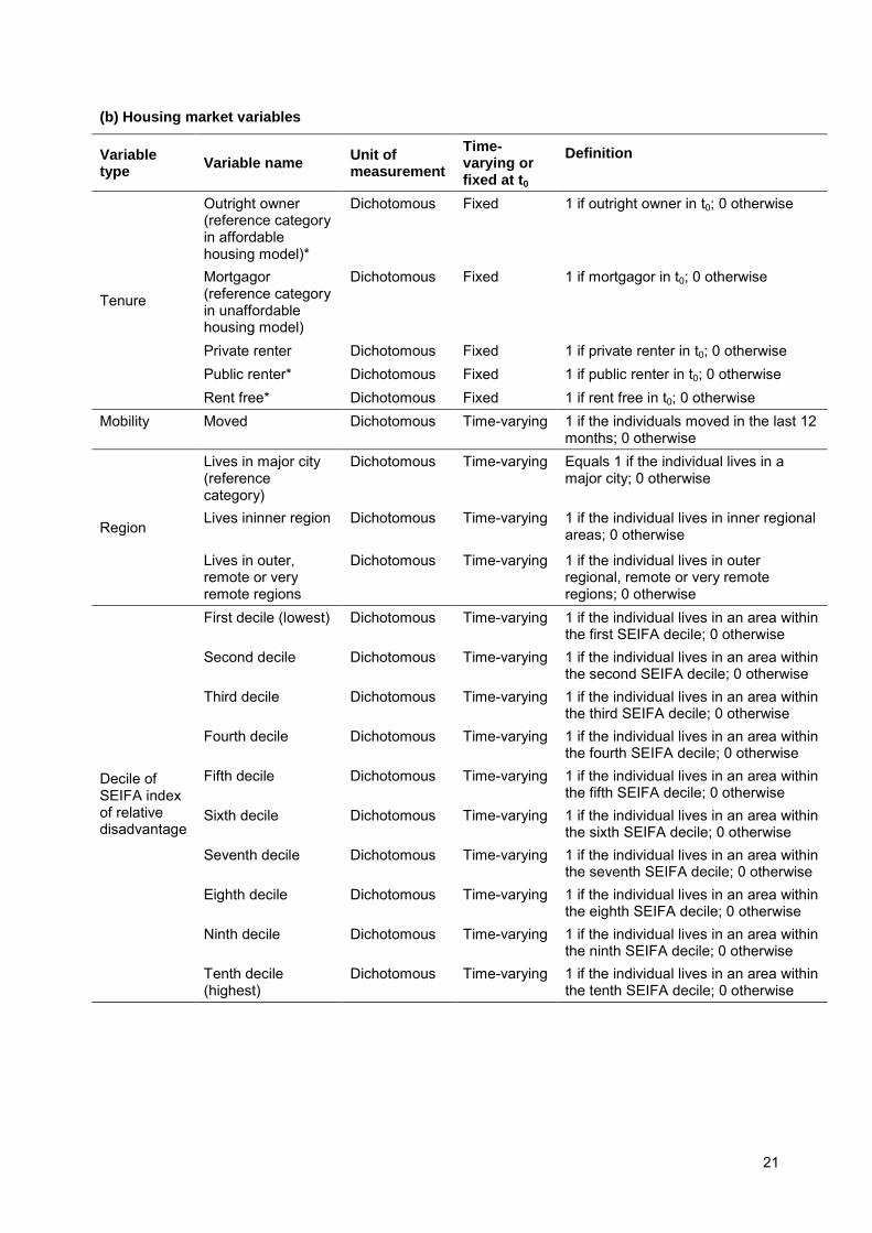
A second group of variables in Table 6 represents features of housing markets, including location. These variables are especially important because they are most likely to yield housing policy relevant inferences. A person’s housing tenure is relevant because mortgagor outlays on housing costs will decline if outstanding mortgage debt is paid off (and interest rates do not rise), but tenants must meet rents that typically increase over time. However, there is a caveat here. Mortgagors have in recent decades become adept at using flexible mortgage products to make in situ withdrawals of housing equity (Ong et al. 2013; Wood et al. 2013). Cost of living pressures can prompt owners to dip into their housing equity in order to meet pressing spending needs, and rising mortgage debt rather than declines is a likely consequence.

While private rental tenants will typically experience increases in rents as their time in the tenure unfolds, there is protection in the form of Commonwealth rent assistance. Geography matters when there is spatial variation in housing prices and rents; in urban areas, prices and rents are generally higher because superior access to amenities and jobs inflates land values. We have made a potentially important change to the way we represent location as compared to the 2009 version of the hazard model described in Wood and Ong (2009). The socio-economic profile of neighbourhoods can influence the opportunities and behaviour of residents

15 Some will nevertheless transition out of affordable housing despite the 25 per cent threshold because of differences between our measure of income and that adopted by the state housing authority.

19

in both positive and negative ways (Rossi-Hansberg et al. 2010). The external effects could help shape the duration of residents’ experiences of housing affordability independently of

residents’ personal characteristics. To take this possibility into account, we have experimented

with four alternative versions of the Australian Bureau of Statistic’s SEIFA index.16 Broadly speaking, these indices rank areas according to their socio-economic status, before grouping ranked areas into 10 deciles; the higher the index (and decile), the higher the socio-economic status of the area.17 In this chapter, we report results based on the deciles of the SEIFA index of relative socio-economic disadvantage, as the impacts do not vary significantly across the four alternative measures.

In our 2009 research project we found that mobility was a strong influence on both the chances of evading housing affordability stress as well as the odds of tumbling out of affordable housing (see Wood & Ong 2009, Tables 18 and 19). As in Wood and Ong (2009.), it is again represented by a dummy variable signalling whether a residential move occurred.

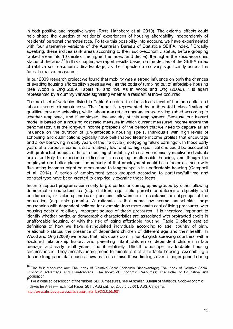
The next set of variables listed in Table 6 capture the individual’s level of human capital and

labour market circumstances. The former is represented by a three-fold classification of qualifications and schooling, while labour market circumstances are distinguished according to whether employed, and if employed, the security of this employment. Because our hazard model is based on a housing cost ratio measure in which current measured income enters the denominator, it is the long-run income prospects of the person that we need to capture as an influence on the duration of (un-)affordable housing spells. Individuals with high levels of schooling and qualifications typically have bell-shaped lifetime income profiles that encourage and allow borrowing in early years of the life cycle (‘mortgaging future earnings’). In those early

years of a career, income is also relatively low, and so high qualifications could be associated with protracted periods of time in housing affordability stress. Economically inactive individuals are also likely to experience difficulties in escaping unaffordable housing, and though the employed are better placed, the security of that employment could be a factor as those with fluctuating incomes might be more prone to lengthy spells in unaffordable housing (Campbell et al. 2014). A series of employment types grouped according to part-time/full-time and contract type have been created to empirically examine these ideas.

Income support programs commonly target particular demographic groups by either allowing demographic characteristics (e.g. children, age, sole parent) to determine eligibility and entitlements, or tailoring particular pensions, allowances or assistance to subgroups of the population (e.g. sole parents). A rationale is that some low-income households, large households with dependent children for example, face more acute cost of living pressures, with housing costs a relatively important source of those pressures. It is therefore important to identify whether particular demographic characteristics are associated with protracted spells in unaffordable housing, or with the risk of losing affordable housing. Table 6 offers detailed definitions of how we have distinguished individuals according to age, country of birth, relationship status, the presence of dependent children of different age and their health. In Wood and Ong (2009) we report that individuals born in non-English speaking countries, with a fractured relationship history, and parenting infant children or dependent children in late teenage and early adult years, find it relatively difficult to escape unaffordable housing circumstances. They are also more prone to tumble out of affordable housing. Assembling a decade-long panel data base allows us to scrutinise these findings over a longer period during 16 The four measures are: The Index of Relative Socio-Economic Disadvantage; The Index of Relative Socio-Economic Advantage and Disadvantage; The Index of Economic Resources; The Index of Education and Occupation. 17 For a detailed description of the various SEIFA measures, see Australian Bureau of Statistics. Socio-economic Indexes for Areas—Technical Paper, 2011, ABS cat. no. 2033.0.55.001, ABS, Canberra, http://www.abs.gov.au/ausstats/abs@.nsf/mf/2033.0.55.001

20

which economic and housing market conditions have fluctuated, and welfare programs have become more tightly targeted.

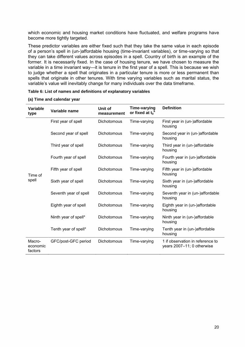
These predictor variables are either fixed such that they take the same value in each episode of a person’s spell in (un-)affordable housing (time-invariant variables), or time-varying so that they can take different values across episodes in a spell. Country of birth is an example of the former. It is necessarily fixed. In the case of housing tenure, we have chosen to measure the variable in a time invariant way—it is tenure in the first year of a spell. This is because we wish to judge whether a spell that originates in a particular tenure is more or less permanent than spells that originate in other tenures. With time varying variables such as marital status, the variable’s value will inevitably change for many individuals over the data timeframe.

Table 6: List of names and definitions of explanatory variables

(a) Time and calendar year

Variable type

Variable name Unit of measurement

Time-varying or fixed at t0

a Definition

Time of spell

First year of spell Dichotomous Time-varying First year in (un-)affordable housing

Second year of spell Dichotomous Time-varying Second year in (un-)affordable housing

Third year of spell Dichotomous Time-varying Third year in (un-)affordable housing

Fourth year of spell Dichotomous Time-varying Fourth year in (un-)affordable housing

Fifth year of spell Dichotomous Time-varying Fifth year in (un-)affordable housing

Sixth year of spell Dichotomous Time-varying Sixth year in (un-)affordable housing

Seventh year of spell Dichotomous Time-varying Seventh year in (un-)affordable housing

Eighth year of spell Dichotomous Time-varying Eighth year in (un-)affordable housing

Ninth year of spell* Dichotomous Time-varying Ninth year in (un-)affordable housing

Tenth year of spell* Dichotomous Time-varying Tenth year in (un-)affordable housing

Macro-economic factors

GFC/post-GFC period Dichotomous Time-varying 1 if observation in reference to years 2007–11; 0 otherwise

21

(b) Housing market variables

Variable type

Variable name Unit of measurement

Time-varying or fixed at t0

Definition

Tenure

Outright owner (reference category in affordable housing model)*

Dichotomous Fixed 1 if outright owner in t0; 0 otherwise

Mortgagor (reference category in unaffordable housing model)

Dichotomous Fixed 1 if mortgagor in t0; 0 otherwise

Private renter Dichotomous Fixed 1 if private renter in t0; 0 otherwise Public renter* Dichotomous Fixed 1 if public renter in t0; 0 otherwise Rent free* Dichotomous Fixed 1 if rent free in t0; 0 otherwise

Mobility Moved Dichotomous Time-varying 1 if the individuals moved in the last 12 months; 0 otherwise

Region

Lives in major city (reference category)

Dichotomous Time-varying Equals 1 if the individual lives in a major city; 0 otherwise

Lives ininner region

Dichotomous Time-varying 1 if the individual lives in inner regional areas; 0 otherwise

Lives in outer, remote or very remote regions

Dichotomous Time-varying 1 if the individual lives in outer regional, remote or very remote regions; 0 otherwise

Decile of SEIFA index of relative disadvantage

First decile (lowest) Dichotomous Time-varying 1 if the individual lives in an area within the first SEIFA decile; 0 otherwise

Second decile Dichotomous Time-varying 1 if the individual lives in an area within the second SEIFA decile; 0 otherwise

Third decile Dichotomous Time-varying 1 if the individual lives in an area within the third SEIFA decile; 0 otherwise

Fourth decile Dichotomous Time-varying 1 if the individual lives in an area within the fourth SEIFA decile; 0 otherwise

Fifth decile Dichotomous Time-varying 1 if the individual lives in an area within the fifth SEIFA decile; 0 otherwise

Sixth decile Dichotomous Time-varying 1 if the individual lives in an area within the sixth SEIFA decile; 0 otherwise

Seventh decile Dichotomous Time-varying 1 if the individual lives in an area within the seventh SEIFA decile; 0 otherwise

Eighth decile Dichotomous Time-varying 1 if the individual lives in an area within the eighth SEIFA decile; 0 otherwise

Ninth decile Dichotomous Time-varying 1 if the individual lives in an area within the ninth SEIFA decile; 0 otherwise

Tenth decile (highest)

Dichotomous Time-varying 1 if the individual lives in an area within the tenth SEIFA decile; 0 otherwise

22

(c) Human capital and labour market variables

Variable type

Variable name Unit of measurement

Time-varying or fixed at t0

Definition

Educational attainment

High-level qualifications (reference category)

Dichotomous Time-varying 1 if individual has a Bachelors degree, Graduate Diploma or Postgraduate Diploma; 0 otherwise

Medium-level qualifications

Dichotomous Time-varying 1 if individual has an (Advanced) Diploma or Certificates I to IV; 0 otherwise

Low-level qualifications

Dichotomous Time-varying 1 if individual has a Year-12 Certificate or lower; 0 otherwise

Employment status and contract type

Full-time permanent contract (reference category)

Dichotomous Time-varying 1 if individual is working permanent full- time; 0 otherwise

Full-time fixed-term contract

Dichotomous Time-varying 1 if individual is working fixed-term full- time; 0 otherwise

Part-time permanent contract

Dichotomous Time-varying 1 if individual is working permanent part-time; 0 otherwise

Part-time fixed-term contract

Dichotomous Time-varying 1 if individual is working fixed-term part-time; 0 otherwise

Casual or other contract

Dichotomous Time-varying 1 if individual is casual; 0 otherwise

Self-employed Dichotomous Time-varying 1 if individual is self-employed; 0 otherwise

Unemployed Dichotomous Time-varying 1 if individual is unemployed; 0 otherwise

Not in labour force Dichotomous Time-varying 1 if individual is not in the labour force; 0 otherwise

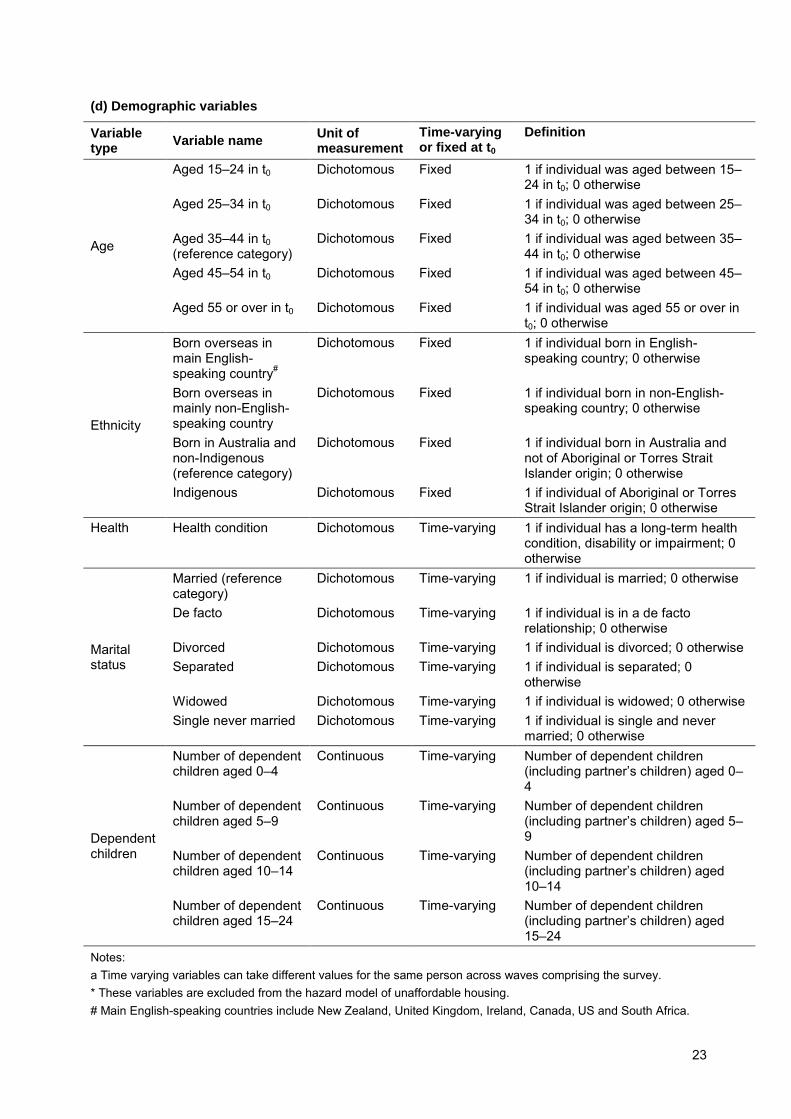
23

(d) Demographic variables

Variable type

Variable name Unit of measurement

Time-varying or fixed at t0

Definition

Age

Aged 15–24 in t0 Dichotomous Fixed 1 if individual was aged between 15–24 in t0; 0 otherwise

Aged 25–34 in t0 Dichotomous Fixed 1 if individual was aged between 25–34 in t0; 0 otherwise

Aged 35–44 in t0 (reference category)

Dichotomous Fixed 1 if individual was aged between 35–44 in t0; 0 otherwise

Aged 45–54 in t0 Dichotomous Fixed 1 if individual was aged between 45–54 in t0; 0 otherwise

Aged 55 or over in t0 Dichotomous Fixed 1 if individual was aged 55 or over in t0; 0 otherwise

Ethnicity

Born overseas in main English-speaking country#

Dichotomous Fixed 1 if individual born in English-speaking country; 0 otherwise

Born overseas in mainly non-English-speaking country

Dichotomous Fixed 1 if individual born in non-English-speaking country; 0 otherwise

Born in Australia and non-Indigenous (reference category)

Dichotomous Fixed 1 if individual born in Australia and not of Aboriginal or Torres Strait Islander origin; 0 otherwise

Indigenous Dichotomous Fixed 1 if individual of Aboriginal or Torres Strait Islander origin; 0 otherwise

Health Health condition Dichotomous Time-varying 1 if individual has a long-term health condition, disability or impairment; 0 otherwise

Marital status

Married (reference category)

Dichotomous Time-varying 1 if individual is married; 0 otherwise

De facto Dichotomous Time-varying 1 if individual is in a de facto relationship; 0 otherwise

Divorced Dichotomous Time-varying 1 if individual is divorced; 0 otherwise Separated Dichotomous Time-varying 1 if individual is separated; 0

otherwise Widowed Dichotomous Time-varying 1 if individual is widowed; 0 otherwise Single never married Dichotomous Time-varying 1 if individual is single and never

married; 0 otherwise

Dependent children

Number of dependent children aged 0–4

Continuous Time-varying Number of dependent children (including partner’s children) aged 0–4

Number of dependent children aged 5–9

Continuous Time-varying Number of dependent children (including partner’s children) aged 5–9

Number of dependent children aged 10–14

Continuous Time-varying Number of dependent children (including partner’s children) aged 10–14

Number of dependent children aged 15–24

Continuous Time-varying Number of dependent children (including partner’s children) aged 15–24

Notes: a Time varying variables can take different values for the same person across waves comprising the survey. * These variables are excluded from the hazard model of unaffordable housing. # Main English-speaking countries include New Zealand, United Kingdom, Ireland, Canada, US and South Africa.

24

3.3 Findings

Table 7 below presents estimates for hazard models of first spells in unaffordable housing. Models 1 and 2 present estimates with and without SEIFA deciles respectively. The inclusion of SEIFA decile variables does not alter the impacts of the other variables in any significant way. Hence, we will discuss the findings of Model 1 first, before scrutinising the effects of the socio-economic profile of neighbourhoods.

Under Model 1, the (conditional) odds of exiting unaffordable housing in the first year of a spell are 6.3 times the odds of exiting during the remaining years of the spell. This estimate is highly significant at the 1 per cent level. In the second year, the odds of exiting unaffordable housing remains high at 3.6 times the odds of exiting during other years of the spell. As per Wood and Ong’s (2009) model, we find strong evidence of negative duration dependence, with the odds

of escaping unaffordable housing exhibiting a sharp decline over the years in both magnitude and statistical significance. 18 By the fourth year, the odds have become statistically insignificant. These findings also confirm the life table patterns in Table 7 of Wood et al. (2014) where we report that the majority of Australians in unaffordable housing circumstances escape into affordable housing within the initial years of the spell.

The dummy variable denoting the (post-)GFC years is statistically insignificant, implying that Australians in unaffordable housing at that time did not find their chances of escape altered by changes in housing and labour market conditions during the GFC. While housing consumers might have experienced some relief in housing costs as a result of easing monetary policy and a slowdown in housing markets (e.g. interest rates fell, paving the way for lower mortgage repayments), there was an offsetting deterioration in labour market circumstances that adversely affected the ability to meet housing cost burdens. However, as we shall learn later in this report, this is the only model in which the GFC variable is statistically insignificant, so it is premature to rule it out as unimportant.

The housing tenure variables suggest that the odds of escaping unaffordable housing are significantly higher for those renting in the private sector at the start of their spell (as compared to a mortgagor).19 That is, those renting at the start of their unaffordable housing spells have odds of exiting that are 1.7 times the odds of mortgagors. On the other hand, the mobility variable is insignificant. In Wood and Ong (2009), the findings were reversed in that the odds of evading unaffordable housing is significantly higher among movers than non-movers, while housing tenure does not appear to have an independent effect on the odds of exiting unaffordable housing. This could be because individuals who begin their spells in unaffordable housing as private renters are more likely to move in order to escape housing affordability stress, so there is some collinearity between the two variables. Home owners who wish to move face higher transaction costs than private renters (principally in the form of stamp duties). These higher transaction costs deter mobility in the home ownership tenure, while private renters who wish to adjust to housing cost pressures by trading down into cheaper housing do not face such constraints.20 Unsurprisingly, residents of inner regional areas find it easier to escape unaffordable housing than those living in major cities where house prices and rents tend to be higher. 18 There is a sharp jump in the magnitude of the odds ratio in the eighth year, and in the case of model 2, this is statistically significant. However, as shown in Table 7 of Wood et al. (2014), very few people remain in the sample after the seventh year of the spell. At the beginning of the eighth year, only eight people remain ‘at risk’ in the sample, resulting in an estimated odds ratio which is spurious in nature. 19 The sample has no outright owners, public renters or persons living in rent-free housing as tenure status is defined in the first wave of a spell in unaffordable housing, and housing costs of outright owners, public renters and persons living in rent free housing are affordable in all waves where this tenure status is applicable. 20 The Spearman’s rank correlation coefficient between the mover and private renter variables is 0.287 and statistically significant at the 1 per cent level. Further analysis also indicates that among those who entered the sample in private rental, around 30 per cent moved residence at least once over the sample timeframe as compared to 7 per cent for individuals who entered the sample as mortgagors.

25

Education qualifications are generally unimportant. While employment security, as proxied by contract type, does not appear to affect the odds of escaping unaffordable housing, employment status is important. Those who are unemployed and not in the labour force have odds of exiting unaffordable housing that are 55 per cent and 40 per cent lower than the odds of full-time employed Australians on permanent contracts (the reference category). Moreover, the self-employed also have significantly reduced chances of escaping unaffordable housing as compared to the reference category. Self-employed individuals typically have lower incomes than those employed on job contracts. In the sample of unaffordable housing spells, we find that mean income unit disposable incomes are approximately $51 000 during episodes of self-employment, as compared to $74 000 during episodes of employment with an employer.

Among the demographic variables, ethnicity has a significant impact on the odds of escaping unaffordable housing. Those born overseas in non-English-speaking countries have odds of escaping that are 35 per cent lower than Australian-born non-Indigenous persons. Similar findings were reported by Wood and Ong (2009) in their model of exits from unaffordable housing over a shorter timeframe. It may be due to discrimination against non-English-speaking minority groups in Australian housing markets. Alternatively, households’ ability to

secure accurate information on housing market conditions such as prices, rents, available vacancies etc. may be constrained by the extent to which people interact socially across ethnic boundaries (Rosenbaum 1992). However, further research is required to ascertain the channels through which ethnicity influences persistent housing affordability stress. There are no statistically significant differences between Indigenous and non-Indigenous Australians, though this finding may be attributed to small sample numbers in the case of Indigenous persons (nine episodes only).

Couples (whether legally married or in de facto relationships) find it easier to escape unaffordable housing than singles who are never married, or who have experienced marital breakdown through separation or divorce. This is likely due to the pooling of resources and economies of scale in (housing) consumption that are available to couples but not singles. Furthermore, separation or divorce can eat into accumulated wealth and disrupt income flows, hence depressing the chances of escape from unaffordable housing.

The presence of very young dependent children is particularly important.21 Each additional child aged 0–4 lowers the odds of exiting unaffordable housing by 45 per cent. When interpreted in conjunction with the marital status variables, it would appear that sole parents are particularly vulnerable to prolonged periods in housing affordability stress. Interestingly, the presence of adult dependent children aged 15–24 years also depress the odds of escaping unaffordable housing, by some 35 per cent. It may be that households with adult dependent children face greater space constraints than those with younger children that prevent trading down into a smaller home to relieve housing cost pressures. For instance, adult dependent children are more likely to require separate bedrooms than younger children. In the case of very young children (up to age 4) the household is likely to experience what might be a temporary reduction in income, as (typically) female partners leave or reduce their participation in the labour market.

The above demographic variables offer helpful insights into the types of households that are most vulnerable to protracted spells of exposure to housing affordability stress. But it would seem that one set of demographics—the age variables representing different stages of the life cycle—are unimportant, as each of the age variables is statistically insignificant. The findings suggest that factors other than age shape the chances of climbing out of unaffordable housing circumstances. This does not mean that the odds of exit do not vary across the life cycle; it

21 In Wood and Ong (2009), the presence of dependent children across all age ranges was found to be important. However, the 2009 study was based upon the 30 per cent rule rather than the 30/40 rule.

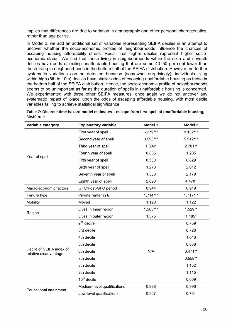
26

implies that differences are due to variation in demographic and other personal characteristics, rather than age per se.

In Model 2, we add an additional set of variables representing SEIFA deciles in an attempt to uncover whether the socio-economic profiles of neighbourhoods influence the chances of escaping housing affordability stress. Recall that higher deciles represent higher socio-economic status. We find that those living in neighbourhoods within the sixth and seventh deciles have odds of exiting unaffordable housing that are some 40–50 per cent lower than those living in neighbourhoods in the bottom half of the SEIFA distribution. However, no further systematic variations can be detected because (somewhat surprisingly), individuals living within high (8th to 10th) deciles have similar odds of escaping unaffordable housing as those in the bottom half of the SEIFA distribution. Hence, the socio-economic profile of neighbourhoods seems to be unimportant as far as the duration of spells in unaffordable housing is concerned. We experimented with three other SEIFA measures; once again we do not uncover any systematic impact of ‘place’ upon the odds of escaping affordable housing, with most decile variables failing to achieve statistical significance.

Table 7: Discrete time hazard model estimates—escape from first spell of unaffordable housing,

30:40 rule

Variable category Explanatory variable Model 1 Model 2

Year of spell

First year of spell 6.279*** 9.132***

Second year of spell 3.593*** 5.512***

Third year of spell 1.839* 2.701**

Fourth year of spell 0.805 1.205

Fifth year of spell 0.530 0.829

Sixth year of spell 1.278 2.012

Seventh year of spell 1.330 2.179

Eighth year of spell 2.690 4.470*

Macro-economic factors GFC/Post-GFC period 0.944 0.919

Tenure type Private renter in t0 1.714*** 1.717***

Mobility Moved 1.120 1.122

Region Lives in Inner region 1.563*** 1.529**

Lives in outer region 1.375 1.485*

Decile of SEIFA index of relative disadvantage

2nd decile

N/A

0.789

3rd decile 0.728

4th decile 1.046

5th decile 0.836

6th decile 0.471**

7th decile 0.558**

8th decile 1.152

9th decile 1.115

10th decile 0.609

Educational attainment Medium-level qualifications 0.996 0.996

Low-level qualifications 0.807 0.764

27

Variable category Explanatory variable Model 1 Model 2

Labour market status

Full-time fixed-term contract

1.232 1.142

Part-time permanent contract

1.216 1.199

Part-time fixed-term contract

0.695 0.737

Casual or other contract 0.851 0.833

Self-employed 0.571*** 0.566***

Unemployed 0.448* 0.483*

Not in labour force 0.596** 0.568***

Age

Aged 15–24 in t0 1.505 1.591

Aged 25–34 in t0 1.331 1.326

Aged 45–54 in t0 1.183 1.252

Aged 55 or over in t0 0.970 0.991

Ethnicity

Born overseas in English-speaking country

0.855 0.813

Born overseas in non-English-speaking country

0.654** 0.612**

Indigenous 0.344 0.305

Health Ill health 0.887 0.907

Marital status

De facto 1.116 1.069

Divorced 0.588* 0.542**

Separated 0.523** 0.480**

Widowed 1.411 1.262

Single, never married 0.490*** 0.419***

Dependent children

Number of dependent children aged 0–4

0.546*** 0.519***

Number of dependent children aged 5–9

1.023 1.036

Number of dependent children aged 10–14

0.963 0.931

Number of dependent children aged 15–24

0.649*** 0.660***

No. of persons 1,338 1,338

Chi-square 331.76*** 350.39***

Notes: *** p<0.01, ** p<0.05, * p<0.1. Reference categories are Mortgagor, Major City, 1st SEIFA decile, Aged 35–

44 in t0, Born in Australia, Married, High-level qualifications and Full-time permanent contract.

Next, we report estimates from hazard models of first spells in affordable housing (see Table 8 below). Here, the event refers to a transition out of affordable housing and therefore into unaffordable housing.22 Once again, we present two models, one without and the other with 22 In this model outright owners, rent free and public housing tenants are present in the sample.

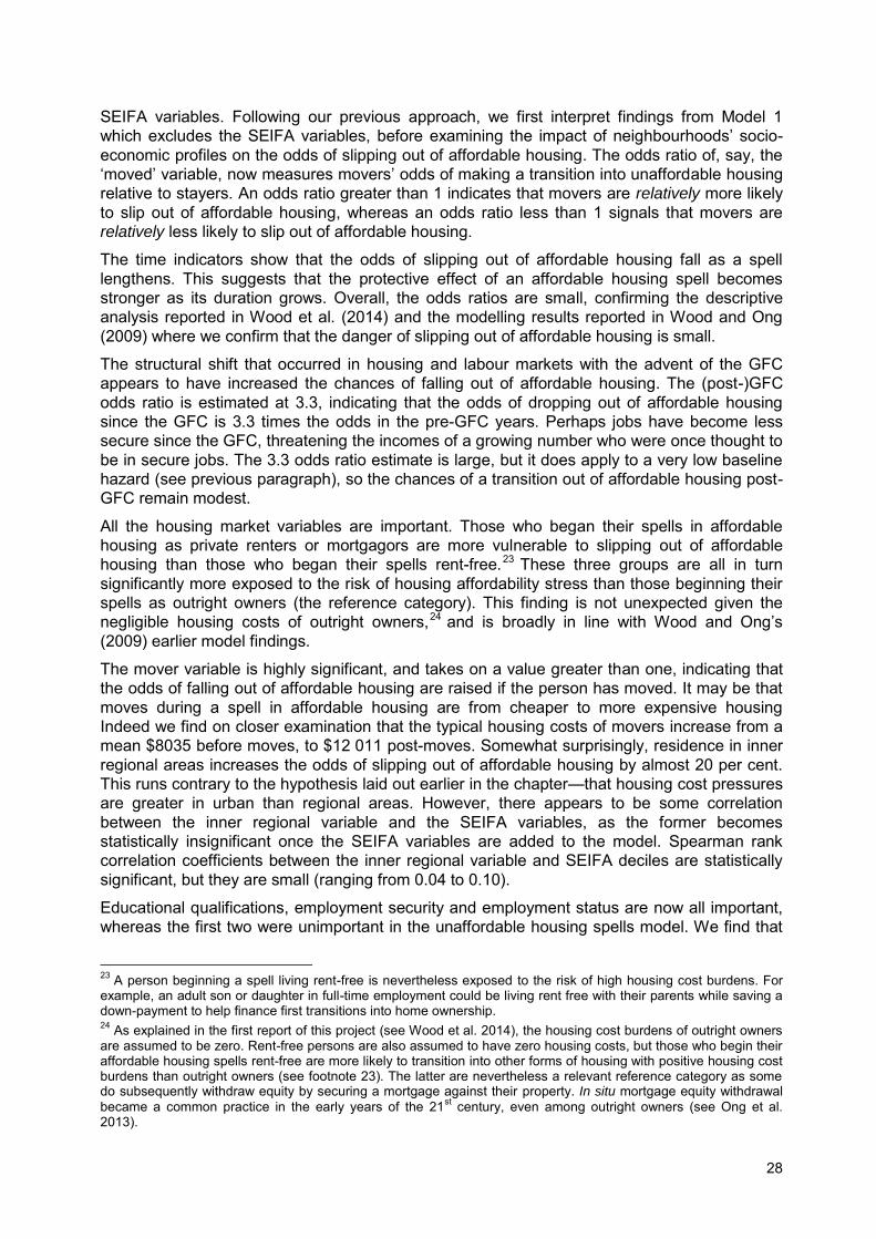
28

SEIFA variables. Following our previous approach, we first interpret findings from Model 1 which excludes the SEIFA variables, before examining the impact of neighbourhoods’ socio-economic profiles on the odds of slipping out of affordable housing. The odds ratio of, say, the ‘moved’ variable, now measures movers’ odds of making a transition into unaffordable housing relative to stayers. An odds ratio greater than 1 indicates that movers are relatively more likely to slip out of affordable housing, whereas an odds ratio less than 1 signals that movers are relatively less likely to slip out of affordable housing.

The time indicators show that the odds of slipping out of affordable housing fall as a spell lengthens. This suggests that the protective effect of an affordable housing spell becomes stronger as its duration grows. Overall, the odds ratios are small, confirming the descriptive analysis reported in Wood et al. (2014) and the modelling results reported in Wood and Ong (2009) where we confirm that the danger of slipping out of affordable housing is small.

The structural shift that occurred in housing and labour markets with the advent of the GFC appears to have increased the chances of falling out of affordable housing. The (post-)GFC odds ratio is estimated at 3.3, indicating that the odds of dropping out of affordable housing since the GFC is 3.3 times the odds in the pre-GFC years. Perhaps jobs have become less secure since the GFC, threatening the incomes of a growing number who were once thought to be in secure jobs. The 3.3 odds ratio estimate is large, but it does apply to a very low baseline hazard (see previous paragraph), so the chances of a transition out of affordable housing post-GFC remain modest.

All the housing market variables are important. Those who began their spells in affordable housing as private renters or mortgagors are more vulnerable to slipping out of affordable housing than those who began their spells rent-free.23 These three groups are all in turn significantly more exposed to the risk of housing affordability stress than those beginning their spells as outright owners (the reference category). This finding is not unexpected given the negligible housing costs of outright owners,24 and is broadly in line with Wood and Ong’s (2009) earlier model findings.

The mover variable is highly significant, and takes on a value greater than one, indicating that the odds of falling out of affordable housing are raised if the person has moved. It may be that moves during a spell in affordable housing are from cheaper to more expensive housing Indeed we find on closer examination that the typical housing costs of movers increase from a mean $8035 before moves, to $12 011 post-moves. Somewhat surprisingly, residence in inner regional areas increases the odds of slipping out of affordable housing by almost 20 per cent. This runs contrary to the hypothesis laid out earlier in the chapter—that housing cost pressures are greater in urban than regional areas. However, there appears to be some correlation between the inner regional variable and the SEIFA variables, as the former becomes statistically insignificant once the SEIFA variables are added to the model. Spearman rank correlation coefficients between the inner regional variable and SEIFA deciles are statistically significant, but they are small (ranging from 0.04 to 0.10).

Educational qualifications, employment security and employment status are now all important, whereas the first two were unimportant in the unaffordable housing spells model. We find that

23 A person beginning a spell living rent-free is nevertheless exposed to the risk of high housing cost burdens. For example, an adult son or daughter in full-time employment could be living rent free with their parents while saving a down-payment to help finance first transitions into home ownership. 24 As explained in the first report of this project (see Wood et al. 2014), the housing cost burdens of outright owners are assumed to be zero. Rent-free persons are also assumed to have zero housing costs, but those who begin their affordable housing spells rent-free are more likely to transition into other forms of housing with positive housing cost burdens than outright owners (see footnote 23). The latter are nevertheless a relevant reference category as some do subsequently withdraw equity by securing a mortgage against their property. In situ mortgage equity withdrawal became a common practice in the early years of the 21st century, even among outright owners (see Ong et al. 2013).

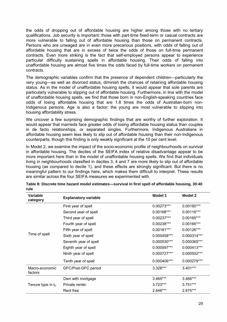
29

the odds of dropping out of affordable housing are higher among those with no tertiary qualifications. Job security is important; those with part-time fixed-term or casual contracts are more vulnerable to falling out of affordable housing than those on permanent contracts. Persons who are unwaged are in even more precarious positions, with odds of falling out of affordable housing that are in excess of twice the odds of those on full-time permanent contracts. Even more striking is the fact that self-employed persons appear to experience particular difficulty sustaining spells in affordable housing. Their odds of falling into unaffordable housing are almost five times the odds faced by full-time workers on permanent contracts.

The demographic variables confirm that the presence of dependent children—particularly the very young—as well as divorced status, diminish the chances of retaining affordable housing status. As in the model of unaffordable housing spells, it would appear that sole parents are particularly vulnerable to slipping out of affordable housing. Furthermore, in line with the model of unaffordable housing spells, we find that those born in non-English-speaking countries face odds of losing affordable housing that are 1.8 times the odds of Australian-born non-Indigenous persons. Age is also a factor; the young are most vulnerable to slipping into housing affordability stress.

We uncover a few surprising demographic findings that are worthy of further exploration. It would appear that marrieds face greater odds of losing affordable housing status than couples in de facto relationships, or separated singles. Furthermore, Indigenous Australians in affordable housing seem less likely to slip out of affordable housing than their non-Indigenous counterparts, though this finding is only weakly significant at the 10 per cent level.

In Model 2, we examine the impact of the socio-economic profile of neighbourhoods on survival in affordable housing. The deciles of the SEIFA index of relative disadvantage appear to be more important here than in the model of unaffordable housing spells. We find that individuals living in neighbourhoods classified in deciles 3, 4 and 7 are more likely to slip out of affordable housing (as compared to decile 1), and these effects are strongly significant. But there is no meaningful pattern to our findings here, which makes them difficult to interpret. These results are similar across the four SEIFA measures we experimented with.

Table 8: Discrete time hazard model estimates—survival in first spell of affordable housing, 30:40

rule

Variable category

Explanatory variable Model 1 Model 2

Time of spell

First year of spell 0.00273*** 0.00190*** Second year of spell 0.00168*** 0.00116*** Third year of spell 0.00237*** 0.00165*** Fourth year of spell 0.00238*** 0.00166*** Fifth year of spell 0.00181*** 0.00126*** Sixth year of spell 0.000458*** 0.000314*** Seventh year of spell 0.000530*** 0.000365*** Eighth year of spell 0.000597*** 0.000413*** Ninth year of spell 0.000727*** 0.000502***

Tenth year of spell 0.000406*** 0.000279***

Macro-economic factors

GFC/Post-GFC period 3.328*** 3.401***

Tenure type in t0 Own with mortgage 3.465*** 3.466*** Private renter 3.723*** 3.751*** Rent free 2.648*** 2.675***

30

Variable category

Explanatory variable Model 1 Model 2

Mobility Moved 1.836*** 1.833***

Region Lives in Inner region 1.190** 1.146 Lives in outer region 0.756** 0.765**

Decile of SEIFA index of relative disadvantage

2nd decile

1.433* 3rd decile 1.778*** 4th decile 1.840*** 5th decile 1.413* 6th decile 1.280 7th decile 1.844*** 8th decile 1.673** 9th decile 1.231 10th decile 1.259

Educational attainment

Medium-level qualifications 1.425*** 1.378*** Low-level qualifications 1.300*** 1.267**

Labour market status

Full-time fixed-term contract 0.750 0.768 Part-time permanent contract 1.573*** 1.581*** Part-time fixed-term contract 2.061** 2.029** Casual or other contract 1.899*** 1.917*** Self-employed 4.817*** 4.868*** Unemployed 2.491*** 2.494*** Not in labour force 3.215*** 3.257***

Age

Aged 15–24 in t0 1.878*** 1.857*** Aged 25–34 in t0 1.338*** 1.331*** Aged 45–54 in t0 0.967 0.972 Aged 55 or over in t0 0.509*** 0.509***

Ethnicity Born overseas in English-speaking country 1.166 1.184 Born overseas in non-English-speaking country 1.829*** 1.841*** Indigenous 0.464* 0.496

Health Ill health 1.114 1.118

Marital status

De facto 0.645*** 0.629*** Divorced 1.984*** 1.958*** Separated 0.532*** 0.514*** Widowed 0.821 0.819 Single, never married 0.758 0.757

Dependent children

Number of dependent children aged 0–4 1.634*** 1.647*** Number of dependent children aged 5–9 1.438*** 1.446*** Number of dependent children aged 10–14 1.183*** 1.183*** Number of dependent children aged 15–24 1.467*** 1.464***

No. of persons 44,009 44,009 Chi-square 10094.18 10121.07***

Notes: *** p<0.01, ** p<0.05, * p<0.1; Reference categories are Outright owners, Major City, 1st SEIFA decile, Aged 35–44 in t0, Born in Australia, Married, High-level qualifications and Full-time permanent contract.

31

3.4 Summary

The models presented in this chapter yield some important findings that are largely in line with Wood and Ong’s (2009) earlier findings. However, the current models extend over a longer

timeframe and thus uncover some interesting new insights.

The models of first spells in unaffordable housing show that most Australians in housing affordability stress escape within a relatively short period of time, though there is evidence of negative duration dependence. Thus, those who fail to exit unaffordable housing quickly find that their chances of escaping housing affordability stress decline sharply as spells lengthen. Mortgagors find it more difficult to manoeuvre out of unaffordable housing than private renters, because the high transaction costs they face impede moves that could ease housing stress. Self- or non-employment also diminish the prospects of evading unaffordable housing circumstances. Sole parents with young dependent children are particularly vulnerable to extended periods in housing affordability stress, as are ethnic groups from non-English-speaking backgrounds. While the study timeframe extends across the GFC and post-GFC years, we do not detect a statistically significant impact. Australians in unaffordable housing were perhaps unable to take advantage of lower interest rates and the slowdown in housing markets during the GFC, because it was accompanied by a parallel decline in labour markets, and thus job security. Area-based socio-economic status, as proxied by SEIFA deciles, appears to have a negligible impact on the odds of escaping unaffordable housing.

The models of survival in affordable housing confirm that the majority of Australians in affordable housing can expect to sustain it. Furthermore, the models uncover a protective effect as spells in affordable housing lengthen. However, ethnic groups from a non-English-speaking background and sole parents with young children are once again more vulnerable, as are self-employed or unwaged persons. Here, job security also becomes important; the odds of surviving in affordable housing is reduced if one is on a part-time fixed-term contract or casual contract. Macro-economic conditions also matter. We find that the chances of sustaining affordable housing have fallen since the GFC.

32

4 ARE SPELLS IN UNAFFORDABLE HOUSING CHARACTERISED BY RELAPSE AND TURBULENCE?

4.1 Introduction

In this chapter we address two issues that extend the analyses conducted in Chapter 3. While the hazard models of first spells in (un-)affordable housing are a helpful guide to the circumstances facilitating an escape from unaffordable housing, or precipitating a fall out of affordable housing, they ignore the future housing affordability profile that unfolds after an escape or fall. The model and sample designs described below redress this omission. We begin by asking whether escapes from unaffordable housing are permanent. Where relapse back into unaffordable housing occurs, the statistical analysis seeks to identify personal characteristics, housing tenure and location features correlated with relapse. This is followed by an investigation of spells in unaffordable housing that are preceded by one or more episodes in affordable housing. Here the focus is on rebounds back into affordable housing circumstances. Once again, we are keen to pin down the personal characteristics, housing tenure and location features correlated with rebounds.

The timeframe for this study is now 10 years (2001–11) and therefore offers an opportunity to describe the stability of housing affordability profiles, and this is the second issue addressed in this chapter. Contemporary housing and labour markets are, in the view of some eminent academics, volatile and individual housing and labour market careers more vulnerable to abrupt and unexpected change (Clapham 2002; Giddens 1990, 1991). Considerable attention has been devoted to the measurement of job security and the variability of earnings profiles in labour studies, but these dynamic perspectives remain relatively undeveloped in housing studies. We aim to make a contribution in this chapter by using the HILDA panel data to explore cycling in and out of housing affordability.

It turns out that these phenomena are of relevance to a large number of Australians. We estimate that of those making escapes from spells of unaffordable housing between 2001 and 2011, 33 per cent relapse back into unaffordable housing at least once by 2011. Using population weights, our calculations indicate that 1.1 million escaped affordability stress, but 408 000 fall back into affordability stress by 2011. Some of these Australians cycle back and forth between unaffordable and affordable housing. Table 9 below measures the number of times the boundaries between unaffordable and affordable housing are crossed by a sample of 875 individuals who have at least one prior completed spell of housing affordability stress. It turns out that 36 per cent transition across these boundaries two or more times between 2001 and 2011. This is equivalent to a population estimate of 388 000 Australians.

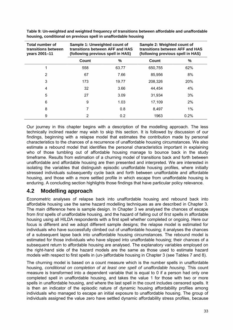
33

Table 9: Un-weighted and weighted frequency of transitions between affordable and unaffordable

housing, conditional on previous spell in unaffordable housing

Total number of transitions between years 2001–11

Sample 1: Unweighted count of transitions between AFF and HAS (following previous spell in HAS)

Sample 2: Weighted count of transitions between AFF and HAS (following previous spell in HAS)

Count % Count %

1 558 63.77 650,755 62%

2 67 7.66 85,956 8%

3 173 19.77 208,326 20%

4 32 3.66 44,454 4%

5 27 3.09 31,934 3%

6 9 1.03 17,109 2%

8 7 0.8 8,497 1%

9 2 0.2 1963 0.2%

Our journey in this chapter begins with a description of the modelling approach. The less technically inclined reader may wish to skip this section. It is followed by discussion of our findings, beginning with a relapse model that estimates the contribution made by personal characteristics to the chances of a recurrence of unaffordable housing circumstances. We also estimate a rebound model that identifies the personal characteristics important in explaining who of those tumbling out of affordable housing manage to bounce back in the study timeframe. Results from estimation of a churning model of transitions back and forth between unaffordable and affordable housing are then presented and interpreted. We are interested in isolating the variables that distinguish episodic unaffordable housing profiles, where initially stressed individuals subsequently cycle back and forth between unaffordable and affordable housing, and those with a more settled profile in which escape from unaffordable housing is enduring. A concluding section highlights those findings that have particular policy relevance.

4.2 Modelling approach

Econometric analyses of relapse back into unaffordable housing and rebound back into affordable housing use the same hazard modelling techniques as are described in Chapter 3. The main difference here is sample design. In Chapter 3 we analysed the chances of escape from first spells of unaffordable housing, and the hazard of falling out of first spells in affordable housing using all HILDA respondents with a first spell whether completed or ongoing. Here our focus is different and we adopt different sample designs; the relapse model is estimated for individuals who have successfully climbed out of unaffordable housing; it analyses the chances of a subsequent lapse back into unaffordable housing circumstances. The rebound model is estimated for those individuals who have slipped into unaffordable housing; their chances of a subsequent return to affordable housing are analysed. The explanatory variables employed on the right-hand side of the hazard models are the same as those used to estimate hazard models with respect to first spells in (un-)affordable housing in Chapter 3 (see Tables 7 and 8).

The churning model is based on a count measure which is the number spells in unaffordable housing, conditional on completion of at least one spell of unaffordable housing. This count measure is transformed into a dependent variable that is equal to 0 if a person had only one completed spell in unaffordable housing, and takes the value 1 for those with two or more spells in unaffordable housing, and where the last spell in the count includes censored spells. It is then an indicator of the episodic nature of dynamic housing affordability profiles among individuals who managed to escape an initial exposure to unaffordable housing. The group of individuals assigned the value zero have settled dynamic affordability stress profiles, because

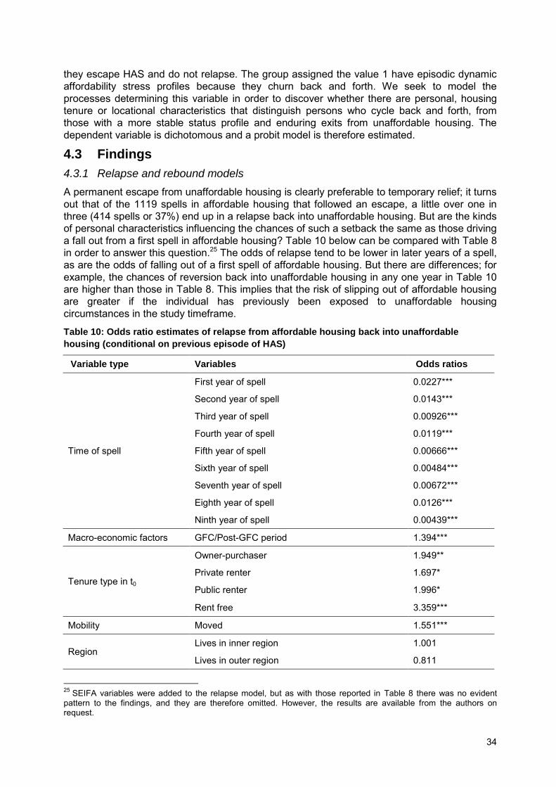
34

they escape HAS and do not relapse. The group assigned the value 1 have episodic dynamic affordability stress profiles because they churn back and forth. We seek to model the processes determining this variable in order to discover whether there are personal, housing tenure or locational characteristics that distinguish persons who cycle back and forth, from those with a more stable status profile and enduring exits from unaffordable housing. The dependent variable is dichotomous and a probit model is therefore estimated.

4.3 Findings

4.3.1 Relapse and rebound models

A permanent escape from unaffordable housing is clearly preferable to temporary relief; it turns out that of the 1119 spells in affordable housing that followed an escape, a little over one in three (414 spells or 37%) end up in a relapse back into unaffordable housing. But are the kinds of personal characteristics influencing the chances of such a setback the same as those driving a fall out from a first spell in affordable housing? Table 10 below can be compared with Table 8 in order to answer this question.25 The odds of relapse tend to be lower in later years of a spell, as are the odds of falling out of a first spell of affordable housing. But there are differences; for example, the chances of reversion back into unaffordable housing in any one year in Table 10 are higher than those in Table 8. This implies that the risk of slipping out of affordable housing are greater if the individual has previously been exposed to unaffordable housing circumstances in the study timeframe.

Table 10: Odds ratio estimates of relapse from affordable housing back into unaffordable

housing (conditional on previous episode of HAS)

Variable type Variables Odds ratios

Time of spell

First year of spell 0.0227***

Second year of spell 0.0143***

Third year of spell 0.00926***

Fourth year of spell 0.0119***

Fifth year of spell 0.00666***

Sixth year of spell 0.00484***

Seventh year of spell 0.00672***

Eighth year of spell 0.0126***

Ninth year of spell 0.00439***

Macro-economic factors GFC/Post-GFC period 1.394***

Tenure type in t0

Owner-purchaser 1.949**

Private renter 1.697*

Public renter 1.996*

Rent free 3.359***

Mobility Moved 1.551***

Region Lives in inner region 1.001

Lives in outer region 0.811

25 SEIFA variables were added to the relapse model, but as with those reported in Table 8 there was no evident pattern to the findings, and they are therefore omitted. However, the results are available from the authors on request.

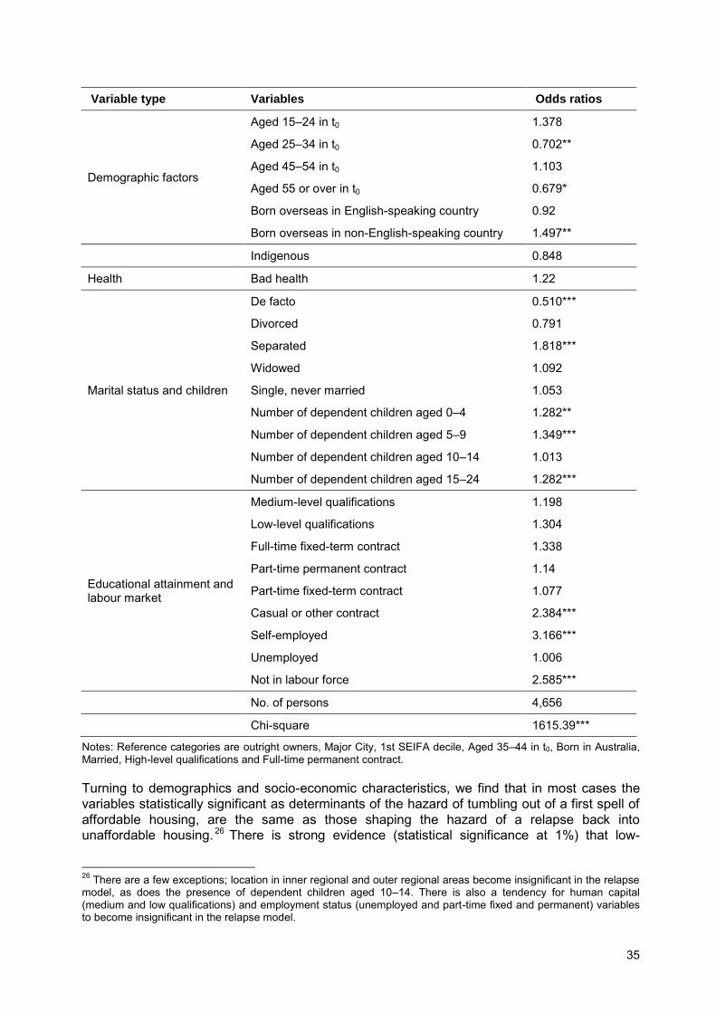
35

Variable type Variables Odds ratios

Demographic factors

Aged 15–24 in t0 1.378

Aged 25–34 in t0 0.702**

Aged 45–54 in t0 1.103

Aged 55 or over in t0 0.679*

Born overseas in English-speaking country 0.92

Born overseas in non-English-speaking country 1.497**

Indigenous 0.848

Health Bad health 1.22

Marital status and children

De facto 0.510***

Divorced 0.791

Separated 1.818***

Widowed 1.092

Single, never married 1.053

Number of dependent children aged 0–4 1.282**

Number of dependent children aged 5–9 1.349***

Number of dependent children aged 10–14 1.013

Number of dependent children aged 15–24 1.282***

Educational attainment and labour market

Medium-level qualifications 1.198

Low-level qualifications 1.304

Full-time fixed-term contract 1.338

Part-time permanent contract 1.14

Part-time fixed-term contract 1.077

Casual or other contract 2.384***

Self-employed 3.166***

Unemployed 1.006

Not in labour force 2.585***

No. of persons 4,656

Chi-square 1615.39***

Notes: Reference categories are outright owners, Major City, 1st SEIFA decile, Aged 35–44 in t0, Born in Australia, Married, High-level qualifications and Full-time permanent contract.

Turning to demographics and socio-economic characteristics, we find that in most cases the variables statistically significant as determinants of the hazard of tumbling out of a first spell of affordable housing, are the same as those shaping the hazard of a relapse back into unaffordable housing. 26 There is strong evidence (statistical significance at 1%) that low-

26 There are a few exceptions; location in inner regional and outer regional areas become insignificant in the relapse model, as does the presence of dependent children aged 10–14. There is also a tendency for human capital (medium and low qualifications) and employment status (unemployed and part-time fixed and permanent) variables to become insignificant in the relapse model.

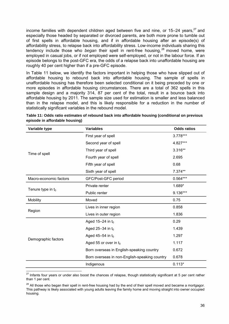
36

income families with dependent children aged between five and nine, or 15–24 years,27 and especially those headed by separated or divorced parents, are both more prone to tumble out of first spells in affordable housing, and if in affordable housing after an episode(s) of affordability stress, to relapse back into affordability stress. Low-income individuals sharing this tendency include those who began their spell in rent-free housing, 28 moved home, were employed in casual jobs, or if not employed were self-employed, or not in the labour force. If an episode belongs to the post-GFC era, the odds of a relapse back into unaffordable housing are roughly 40 per cent higher than if a pre-GFC episode.

In Table 11 below, we identify the factors important in helping those who have slipped out of affordable housing to rebound back into affordable housing. The sample of spells in unaffordable housing has therefore been selected conditional on it being preceded by one or more episodes in affordable housing circumstances. There are a total of 362 spells in this sample design and a majority 314, 87 per cent of the total, result in a bounce back into affordable housing by 2011. The sample size used for estimation is smaller and less balanced than in the relapse model, and this is likely responsible for a reduction in the number of statistically significant variables in the rebound model.

Table 11: Odds ratio estimates of rebound back into affordable housing (conditional on previous

episode in affordable housing)

Variable type Variables Odds ratios

Time of spell

First year of spell 3.778***

Second year of spell 4.827***

Third year of spell 3.316**

Fourth year of spell 2.695

Fifth year of spell 0.68

Sixth year of spell 7.374**

Macro-economic factors GFC/Post-GFC period 0.564***

Tenure type in t0 Private renter 1.689*

Public renter 9.136***

Mobility Moved 0.75

Region Lives in inner region 0.858

Lives in outer region 1.836

Demographic factors

Aged 15–24 in t0 0.29

Aged 25–34 in t0 1.439

Aged 45–54 in t0 1.297

Aged 55 or over in t0 1.117

Born overseas in English-speaking country 0.672

Born overseas in non-English-speaking country 0.678

Indigenous 0.113*

27 Infants four years or under also boost the chances of relapse, though statistically significant at 5 per cent rather than 1 per cent. 28 All those who began their spell in rent-free housing had by the end of their spell moved and became a mortgagor. This pathway is likely associated with young adults leaving the family home and moving straight into owner occupied housing.

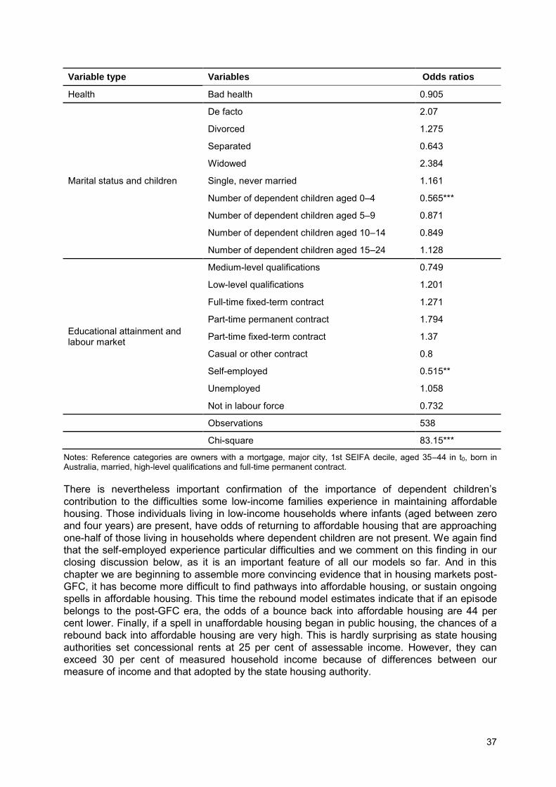
37

Variable type Variables Odds ratios

Health Bad health 0.905

Marital status and children

De facto 2.07

Divorced 1.275

Separated 0.643

Widowed 2.384

Single, never married 1.161

Number of dependent children aged 0–4 0.565***

Number of dependent children aged 5–9 0.871

Number of dependent children aged 10–14 0.849

Number of dependent children aged 15–24 1.128

Educational attainment and labour market

Medium-level qualifications 0.749

Low-level qualifications 1.201

Full-time fixed-term contract 1.271

Part-time permanent contract 1.794

Part-time fixed-term contract 1.37

Casual or other contract 0.8

Self-employed 0.515**

Unemployed 1.058

Not in labour force 0.732

Observations 538

Chi-square 83.15***

Notes: Reference categories are owners with a mortgage, major city, 1st SEIFA decile, aged 35–44 in t0, born in Australia, married, high-level qualifications and full-time permanent contract.

There is nevertheless important confirmation of the importance of dependent children’s

contribution to the difficulties some low-income families experience in maintaining affordable housing. Those individuals living in low-income households where infants (aged between zero and four years) are present, have odds of returning to affordable housing that are approaching one-half of those living in households where dependent children are not present. We again find that the self-employed experience particular difficulties and we comment on this finding in our closing discussion below, as it is an important feature of all our models so far. And in this chapter we are beginning to assemble more convincing evidence that in housing markets post-GFC, it has become more difficult to find pathways into affordable housing, or sustain ongoing spells in affordable housing. This time the rebound model estimates indicate that if an episode belongs to the post-GFC era, the odds of a bounce back into affordable housing are 44 per cent lower. Finally, if a spell in unaffordable housing began in public housing, the chances of a rebound back into affordable housing are very high. This is hardly surprising as state housing authorities set concessional rents at 25 per cent of assessable income. However, they can exceed 30 per cent of measured household income because of differences between our measure of income and that adopted by the state housing authority.

38

4.3.2 Probit model estimates of episodic HAS profiles

The findings section of this chapter is concluded by a systematic analysis of the personal characteristics associated with episodic housing affordability profiles. We employ a person-based sample of observations, where individuals included in the sample for estimation purposes are those who have over the timeframe 2001–11 escaped at least one spell of unaffordable housing. This selection rule generates a sample design of 1012 persons. Note that because of this selection rule, all 1012 persons are drawn from the low-income segment of the income distribution.29 It turns out that more than half (714 persons, 69.3%) of the sample have experienced one spell only. The probit model that we have estimated is based on a dependent variable that assigns the value 1 to those individuals experiencing two or more spells of HAS, and assigns the value 0 otherwise. Since the sample is person rather than person-period based, the time varying explanatory variables are calculated as the percentage of waves in which an indicated personal characteristic is evident. Consider divorce, for example; this variable is the percentage of waves in which a survey participant reports their marital status as divorced. Thus if the respondent responds in the affirmative in every wave the variable takes, the value is 100 per cent. The model aims to offer insights into the personal characteristics of those especially prone to sporadic spells in HAS. It therefore augments the relapse and rebound model analyses by exploring repeated cycling back and forth between affordable and unaffordable housing cost burdens.

Probit model findings are presented in Table 12. In column 2 we list coefficient estimates. We can gauge the direction of each variable’s impact (positive or negative) on the dependent

variable from this coefficient and its statistical significance (or otherwise) is indicated. But probit coefficient estimates by themselves are not easily interpreted and are therefore often coupled with marginal effects estimates, which estimate changes in the (conditional) probability of the outcome variable in response to a unit change in the explanatory variable, ceteris paribus. In the case of dummy variables, it is the predicted change in the (conditional) probability of the outcome variable when the dummy variable switches from zero to one.

The model turns out to have a modest number of statistically significant coefficients, and they offer a modest level of predictive accuracy. Of the 305 individuals with multiple spells of HAS, the model correctly predicts only 30 per cent. Because the dependent variable is unbalanced, there being more individuals with single spells, the model is better at predicting single spells with a much higher 90 per cent successfully assigned by the model. Statistically significant and positive impacts on the propensity to churn back and forth are found for young adults (15–24 years of age), migrants from non-English-speaking backgrounds, the presence of dependent children (age 5–9 years and 15–24 years), the self-employed and those not in the labour force. These variables suggest that younger low-income segments of the population, as well as those with acute spending needs due to growing families, and especially if accompanied by precarious employment, are especially prone to episodic HAS profiles.

29 During their spell of unaffordable housing each person will have equivalised disposable household income that is at or below the 40th percentile of the income distribution.

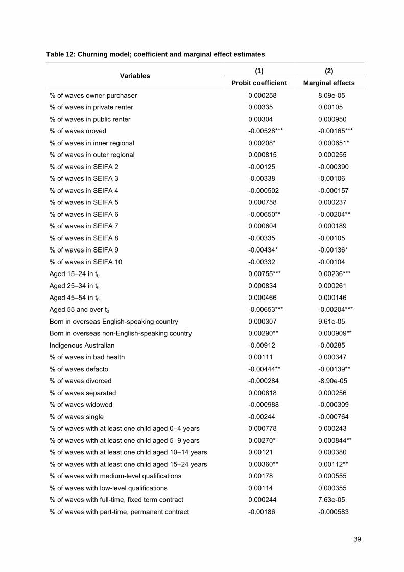
39

Table 12: Churning model; coefficient and marginal effect estimates

Variables (1) (2)

Probit coefficient Marginal effects

% of waves owner-purchaser 0.000258 8.09e-05

% of waves in private renter 0.00335 0.00105

% of waves in public renter 0.00304 0.000950

% of waves moved -0.00528*** -0.00165***

% of waves in inner regional 0.00208* 0.000651*

% of waves in outer regional 0.000815 0.000255

% of waves in SEIFA 2 -0.00125 -0.000390

% of waves in SEIFA 3 -0.00338 -0.00106

% of waves in SEIFA 4 -0.000502 -0.000157

% of waves in SEIFA 5 0.000758 0.000237

% of waves in SEIFA 6 -0.00650** -0.00204**

% of waves in SEIFA 7 0.000604 0.000189

% of waves in SEIFA 8 -0.00335 -0.00105

% of waves in SEIFA 9 -0.00434* -0.00136*

% of waves in SEIFA 10 -0.00332 -0.00104

Aged 15–24 in t0 0.00755*** 0.00236***

Aged 25–34 in t0 0.000834 0.000261

Aged 45–54 in t0 0.000466 0.000146

Aged 55 and over t0 -0.00653*** -0.00204***

Born in overseas English-speaking country 0.000307 9.61e-05

Born in overseas non-English-speaking country 0.00290** 0.000909**

Indigenous Australian -0.00912 -0.00285

% of waves in bad health 0.00111 0.000347

% of waves defacto -0.00444** -0.00139**

% of waves divorced -0.000284 -8.90e-05

% of waves separated 0.000818 0.000256

% of waves widowed -0.000988 -0.000309

% of waves single -0.00244 -0.000764

% of waves with at least one child aged 0–4 years 0.000778 0.000243

% of waves with at least one child aged 5–9 years 0.00270* 0.000844**

% of waves with at least one child aged 10–14 years 0.00121 0.000380

% of waves with at least one child aged 15–24 years 0.00360** 0.00112**

% of waves with medium-level qualifications 0.00178 0.000555

% of waves with low-level qualifications 0.00114 0.000355

% of waves with full-time, fixed term contract 0.000244 7.63e-05

% of waves with part-time, permanent contract -0.00186 -0.000583

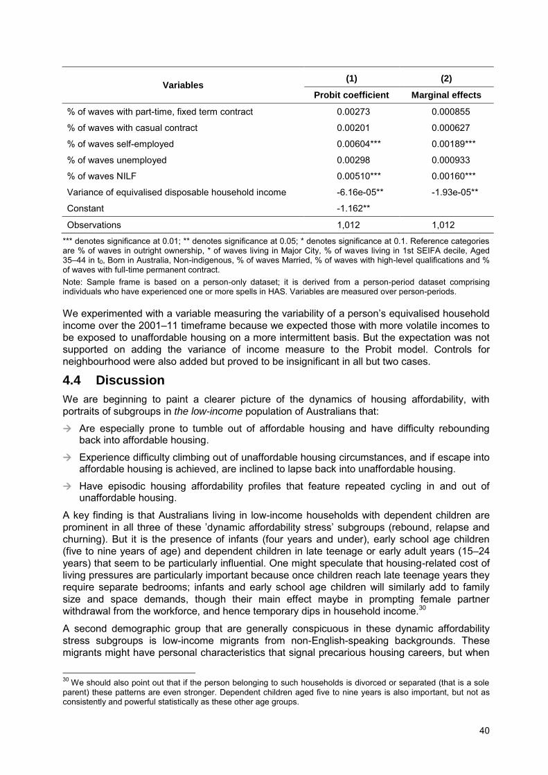
40

Variables (1) (2)

Probit coefficient Marginal effects

% of waves with part-time, fixed term contract 0.00273 0.000855

% of waves with casual contract 0.00201 0.000627

% of waves self-employed 0.00604*** 0.00189***

% of waves unemployed 0.00298 0.000933

% of waves NILF 0.00510*** 0.00160***

Variance of equivalised disposable household income -6.16e-05** -1.93e-05**

Constant -1.162**

Observations 1,012 1,012

*** denotes significance at 0.01; ** denotes significance at 0.05; * denotes significance at 0.1. Reference categories are % of waves in outright ownership, * of waves living in Major City, % of waves living in 1st SEIFA decile, Aged 35–44 in t0, Born in Australia, Non-indigenous, % of waves Married, % of waves with high-level qualifications and % of waves with full-time permanent contract. Note: Sample frame is based on a person-only dataset; it is derived from a person-period dataset comprising individuals who have experienced one or more spells in HAS. Variables are measured over person-periods.

We experimented with a variable measuring the variability of a person’s equivalised household

income over the 2001–11 timeframe because we expected those with more volatile incomes to be exposed to unaffordable housing on a more intermittent basis. But the expectation was not supported on adding the variance of income measure to the Probit model. Controls for neighbourhood were also added but proved to be insignificant in all but two cases.

4.4 Discussion

We are beginning to paint a clearer picture of the dynamics of housing affordability, with portraits of subgroups in the low-income population of Australians that:

Are especially prone to tumble out of affordable housing and have difficulty rebounding back into affordable housing.

Experience difficulty climbing out of unaffordable housing circumstances, and if escape into affordable housing is achieved, are inclined to lapse back into unaffordable housing.

Have episodic housing affordability profiles that feature repeated cycling in and out of unaffordable housing.

A key finding is that Australians living in low-income households with dependent children are prominent in all three of these ’dynamic affordability stress’ subgroups (rebound, relapse and

churning). But it is the presence of infants (four years and under), early school age children (five to nine years of age) and dependent children in late teenage or early adult years (15–24 years) that seem to be particularly influential. One might speculate that housing-related cost of living pressures are particularly important because once children reach late teenage years they require separate bedrooms; infants and early school age children will similarly add to family size and space demands, though their main effect maybe in prompting female partner withdrawal from the workforce, and hence temporary dips in household income.30

A second demographic group that are generally conspicuous in these dynamic affordability stress subgroups is low-income migrants from non-English-speaking backgrounds. These migrants might have personal characteristics that signal precarious housing careers, but when

30 We should also point out that if the person belonging to such households is divorced or separated (that is a sole parent) these patterns are even stronger. Dependent children aged five to nine years is also important, but not as consistently and powerful statistically as these other age groups.

41

we compare this group of migrants with the Australian born (using the full HILDA sample of adults) there is only patchy evidence of this. Migrants from non-English-speaking backgrounds are disproportionately in couple households with dependent children, and are under-represented among the full-time employed; but there is little of note in the occupations they work in, and they are better qualified (30% with bachelor degree or better) than the Australian born (19% with bachelor degree or better). These migrants might find it more difficult to navigate pathways into sustainable affordable housing because of language difficulties, and unfamiliarity with institutional practices in Australian housing markets. Discrimination is also a possible cause.31

Human capital and employment status variables yielded some interesting results. The unemployed are a marked presence in some of the dynamic affordability stress subgroups, but not all.32 Those who are out of the labour force or in employment but working in casual jobs seem more likely to churn, and relapse back into unaffordable housing after achieving a temporarily successful exit from HAS. But it is the self-employed who are consistently over-represented in all forms of dynamic affordability stress groups. They are an intriguing group that have rarely featured as a focus in housing studies, though they represent a sizeable 16 per cent of the employed workforce. On comparing their personal characteristics with the rest of the employed labour force we uncover marked differences.33 The self-employed are significantly older, with a 10-year age difference (47 years versus 37 years) separating them; over two-thirds (69%) are married compared to less than one-half (46%) of the rest of the employed workforce, and there is a striking gender difference with males accounting for two-thirds of the self-employed, but a much lower one-half of the rest of the workforce. Their housing tenure profile is also noticeably different with a concentration of the self-employed in owner occupation.34 Perhaps the most significant marker distinguishing the self-employed is the variable nature of their household disposable incomes, with variance measures of household disposable incomes that are roughly twice as volatile as those in the rest of the workforce.35 It seems likely that the self-employed are disproportionately located at the edges of ownership (Wood et al. 2013), where they juggle spending, saving and mortgage repayment decisions against a backdrop featuring uncertain income streams. One might also speculate that many of the self-employed would prefer permanent full-time employment, but have been made redundant, and find there is a scarcity of such jobs for those in their 40s and 50s.36 The self-employed are a key group as far as future research is concerned, and we take this up further in our final chapter.

We also have important findings beyond those concerning individual demographic and socio-economic attributes. With the longer timeframe available to us in this project we have uncovered more convincing evidence that the GFC matters to at least some housing outcomes. Our econometric model estimates suggest that the chances of falling into dynamic affordability stress groups are higher in the post-GFC years, all else being equal. It seems that navigation out of unaffordable housing and the ability to sustain affordable housing has become more difficult. The channels through which the GFC has precipitated these changes

31 Indigenous persons are not prominent in these three groups as are the overseas born. Small sample numbers are a likely cause. 32 They are absent from the group prone to cycle back and forth between unaffordable and affordable housing; this might reflect enduring spells exposed to high housing cost burdens that are more typical among a group with protracted low income when joblessness persists. 33 As with the descriptive statistics on migrants, our data source is the HILDA sample. A complete set of descriptive statistics is available from the authors on request. 34 Eighty-one per cent (69%) of the self-employed (rest of the workforce) are owner-occupiers. 35 The variance of the self-employed (other workers) disposable household incomes is $3068 ($1453) over the timeframe 2001–11. 36 We are grateful to one of our peer reviewers for pointing this out.

42

are unknown, and it is even conceivable that the GFC is not responsible, but rather other structural factors contemporaneous with the post-GFC years.

Finally, we have an important negative finding to report. In this study we have sought to ascertain whether neighbourhood matters to the dynamics of housing affordability profiles. In the main we have failed to detect a direct influence using ABS SIEFA measures. This does not mean that neighbourhood characteristics are irrelevant; their influence could be indirect, but the evidence offered in this study is unable to detect systematic and direct channels of influence.

These are important and novel findings. Their significance to policy and the future research directions they prompt are taken up in our final chapter.

43

5 POLICY IMPLICATIONS AND FUTURE DIRECTIONS FOR RESEARCH

The dynamics of housing affordability are a neglected subject. But the topic deserves attention. A short exposure to a high housing cost burden that is never repeated is of much less concern than persistent or episodic spells of housing affordability stress. Indeed, when we examine wellbeing measures, there is a clear indication that this distinction matters. In the HILDA sample of private renters, those with one spell of unaffordable housing lasting one year or less have average life satisfaction scores (2001–11) that are 5 per cent or 0.4 points higher than those of private renters with a spell lasting more than one year, or cycling in and out of unaffordable housing two or more times. Similar patterns are evident among mortgagors. Mason et al. 2013 also offer evidence confirming a significant relationship between housing affordability and mental health in Australia.37

The research documented in this report offers key insights into the duration of exposures to unaffordable housing. It also identifies the socio-demographic characteristics of those low-

income Australians who find it more difficult to climb out of unaffordable housing in the first place; and if and when they do evade unaffordable housing, the types of low-income Australians who are more likely to slip back into unaffordable housing. Among low-income Australians, there are three groups that we can describe given the personal characteristics that our econometric modelling has flagged as important identifiers:

Households with dependent children, particularly if there is a lone parent.

Migrants born in non-English-speaking countries.

Working age individuals on the margins of the labour market—the unemployed and those who have dropped out of the labour force—as well as the self-employed.

The cuts to Family Tax Benefit (FTB) in the recent 2014 budget will subject the first group to a greater risk of dynamic housing stress. A key feature is changes to the income free area thresholds of allowance payments for working age individuals, students and parents which will be fixed for three years, while the maximum rates will also be fixed for two years.38 As a consequence, eligible families’ real incomes will fall all else being equal.39 But for families in private rental housing, there are wider consequences because the Commonwealth Rent Assistance (CRA) taper will apply at lower levels of real income than would have been the case under indexation. This is because CRA is only removed once entitlement to the underlying income support payment (that is a ‘passport to’ eligibility) is lost. It will therefore offer families less financial support, a conclusion that is particularly significant in view of findings reported in

37 Mortgagors with one spell of unaffordable housing lasting one year or less have average life satisfaction scores (2001–11) of 7.9, 4 per cent or 0.3 points higher than those of mortgagors with a spell lasting more than one year, or cycling in and out of unaffordable housing two or more times. The life satisfaction score is measured on a scale from 0 (completely dissatisfied) to 10 (completely satisfied). To put these differentials in context, note that those with a long-term disability or illness have mental health levels 10 per cent lower than the rest (Wood et al. 2013). 38 Income-free area thresholds are the levels of assessable income at which income support payments begin to taper off. The three-year freeze on income-free thresholds will affect Newstart Allowance, Widow Allowance, Sickness Allowance, Partner Allowance, Parenting Payment Partnered, Parenting Payment Single, Child Care Benefit, Youth Allowance, Austudy and Abstudy. For more details, refer to http://www.humanservices.gov.au/corporate/publications-and-resources/budget/1415/measures/families/58-000806 39 Other changes to FTB will particularly impact single parents and large families and erode capacity to pay for affordable housing. From 1 July 2015, families whose youngest child is aged six or over will lose entitlement to Family Tax Benefit Part B. However, a new $750 yearly allowance can be accessed by single parent families in receipt of Family Tax Benefit Part A. The allowance will be paid as an additional component of Family Tax Benefit Part A and each child in the family aged between 6 and 12 years of age is eligible for the $750 allowance. Finally, families with three children will no longer receive the large family supplement. For details see http://www.humanservices.gov.au/corporate/publications-and-resources/budget/1415/measures/.

44

this project’s first report that CRA provided a very effective safeguard to eligible clients over the decade 2001–11 (see Wood et. al. 2014).

The Commonwealth Government is likely to look for further savings from the CRA budget as it strives to achieve a budget surplus. The total cost of CRA to the Commonwealth has been increasing at a rapid rate. The Reform of the Federation White Paper reports that 'since 2008–

09, expenditure on CRA has increased by around 33 per cent in real terms, from $2.97 billion in 2008–09 to $3.95 billion in 2013–14, while the number of CRA recipients has increased by 27 per cent, from 1.04 million in 2008–09 to 1.32 million in 2013–14' (Department of the Prime Minister and Cabinet 2014, p.16). That costing will blow out further if CRA is extended to public housing tenants, a reform mooted in the interim June 2014 report of the Reference Group on Welfare Reform. Our research results suggest that a priority in such reform designs is the protection of low-income families, especially those with sole parents, as they appear most vulnerable to dynamic housing stress in contemporary housing markets.

Housing tenure is unsurprisingly an important contextual influence on the duration of exposures to housing affordability stress, as well as individuals’ chances of sustaining

affordable housing once unaffordable housing costs burdens are left behind. We find that public housing provides effective insurance against both protracted and episodic housing affordability stress. This is because it offers low-income tenants certainty with respect to rent payments as a share of gross assessable household income. On the other hand, low-income private rental tenants feature prominently among those with dynamic housing stress, especially if ineligible for CRA. The interim report of the Reference Group on Welfare Reform has flagged radical reform to current arrangements (Reference Group on Welfare Reform 2014, p.71). The reforms would introduce market rents for social housing tenants who would then become eligible for CRA. While introducing a horizontally more equitable set of housing subsidy arrangements, our research findings suggest that a policy initiative of this kind would place public housing tenants at greater risk of protracted and episodic spells of housing affordability stress.

Protracted and episodic housing affordability stress is rare once home buyers attain outright ownership. But pathways into outright ownership are becoming more difficult because first entry into home ownership is being achieved later in life, and younger generations of home owners are regularly tapping into their housing equity to meet pressing spending needs (Wood et al. 2013). We are therefore witnessing falling rates of outright ownership among older Australians. For example, according to the ABS Survey of Income and Housing Costs, back in 1982, 74 per cent or almost three-quarters of 55–64-year old owner-occupiers had paid off their mortgages; by 2012, it had slumped to 58 per cent. The fall is even steeper among 45–

54-year old owner-occupiers, from over one-half (55%) to under one-third (30%). Outright ownership is then offering protection to fewer middle aged and older Australian owner-occupiers than it did 30 years or so ago, and as a result persistent and sporadic housing stress is becoming more common later in the life course. This is a new development in Australia’s

housing system. It poses challenges for Australia’s welfare state given the importance of

outright ownership as a pillar supporting retirement incomes policy (Yates & Bradbury 2010).

There are two especially interesting groups among low-income households that our econometric modelling flag as prone to dynamic affordability stress—migrants born in non-English-speaking countries and the self-employed—that warrant further research before policy prescriptions can be advanced. It is unclear why this subgroup of migrants is vulnerable to protracted and episodic affordability problems. We need further research that can pin down whether housing market discrimination is responsible.

45

The self-employed are a second and intriguing group. They are over-represented among and a rising share of low-income Australians suffering dynamic housing stress.40 Their incomes are much more variable than those of the rest of the workforce, and they are typically paying off mortgages despite an older age profile. They are part of the reason why we are witnessing the encroachment of affordability stress later in Australians’ lives. But whether they represent a

concern for policy is unclear. The self-employed might be a group that regularly add to their mortgages in situ in order to smooth consumption or buffer income shocks. They could be dipping into their housing equity in order to finance business ventures. Whatever the reasons, it is clear that the variability of incomes is likely contributing to their dynamic housing affordability stress. The wider implications of this interesting finding remain to be explored in further research.

40 The proportion of self-employed among the working population in HAS almost doubled over the decade between 2001–11, increasing from 26 per cent in 2001 to 42 per cent in 2011.

46

REFERENCES

Australian Bureau of Statistics (ABS) 1997, Survey of income and housing costs, Australia:

user guide, cat. no. 6553.0, Australian Bureau of Statistics, Canberra.

—— 2011, Socio-economic indexes for areas—technical paper, cat. no. 2033.0.55.001, Australian Bureau of Statistics, Canberra, http://www.abs.gov.au/ausstats/abs@.nsf/mf/2033.0.55.001.

Campbell, I, Parkinson, S & Wood, G A 2014, Underemployment and housing insecurity:an

empirical analysis of HILDA data, Final Report Series, no.230, Australian Housing and Urban Research Institute, Melbourne.

Clapham, D 2002, 'Housing pathways: a post modern analytical framework', Housing, Theory

and Society, vol. 19, no. 2, pp.57–68.

Department of the Prime Minister and Cabinet 2014, Reform of the Federation White Paper

(Roles and responsibilities in housing and homelessness, Issues paper 2, (Australia), viewed 01 February 2015, http://apo.org.au/node/41596.

Doling, J & Elsinga, M 2013, Demographic change and housing wealth; homeowners, pensions

and asset-based welfare in Europe, Springer, Dordrecht. Heidelberg. New York.

Giddens, A 1990, The consequences of modernity, Polity Press, Cambridge.

Giddens, A 1991, Modernity and self identity; self and society in the late modern age, Polity Press, Cambridge.

Mason, K E, Baker, E, Blakely, T & Bentley, R J 2013, 'Housing affordability and mental health: Does the relationship differ for renters and home purchasers?', Social Science &

Medicine, Vol. 94, October, pp.91–97.

O’Flaherty, B. 2004, 'Wrong person and wrong place: for homelessness, the conjunction is

what matters', Journal of Housing Economics, vol. 13, pp.1–15.

Ong, R, Parkinson, S, Searle, B A, Smith, S J & Wood, G A 2013, ‘Channels from housing

wealth to consumption’, Housing Studies, vol. 28, no. 7, pp.1012–1036.

Reference Group on Welfare Reform to the Minister for Social Services 2014, A new system

for better employment and social outcomes interim report, June 2014.

Rosenbaum, E 1992, 'Race and ethnicity in housing: turnover in New York City , 1978–1987', Demography, vol. 29, pp.467–486.

Rossi-Hansberg, E, Sarte, P-D & Owens, R, 2010, 'Housing externalities', Journal of Political

Economy, vol. 118, no. 3, pp.485–535.

Rowley, S, Ong, R & Haffner, M 2014 (published online), 'Bridging the gap between housing stress and financial stress: the case of Australia', Housing Studies, DOI: 10.1080/02673037.2014.977851.

Wood, G & Ong, R 2008, Redesigning AHURI’s Australian housing market microsimulation

model, Final Report, November, Australian Housing and Urban Research Institute, Melbourne.

—— 2009, The dynamics of housing affordability: movements in and out of housing

affordability stress 2001–06, AHURI Final Report no. 133, Australian Housing and Urban Research Institute, Melbourne.

Wood, G, Ong, R & Cigdem, M 2014, Housing affordability dynamics; new insights from the

last decade, AHURI Final Report no. 233, Australian Housing and Urban Research Institute, Melbourne.

47

Wood, G, Parkinson, S, Ong, R, Searle, B A & Smith, S J 2013, Motivations for equity

borrowing: a welfare switching effect, Urban Studies, vol. 50, no. 12, pp.2588–2607.

Wood, G, Smith, S, Ong, R & Cigdem, M 2013, The edges of home ownership, AHURI Final Report no. 216, Australian Housing and Urban Research Institute, Melbourne.

Yates, J & Bradbury, B 2010, 'Home ownership as a (crumbling) fourth pillar of social insurance in Australia', Journal of Housing and the Built Environment, vol. 25, pp.193–211.

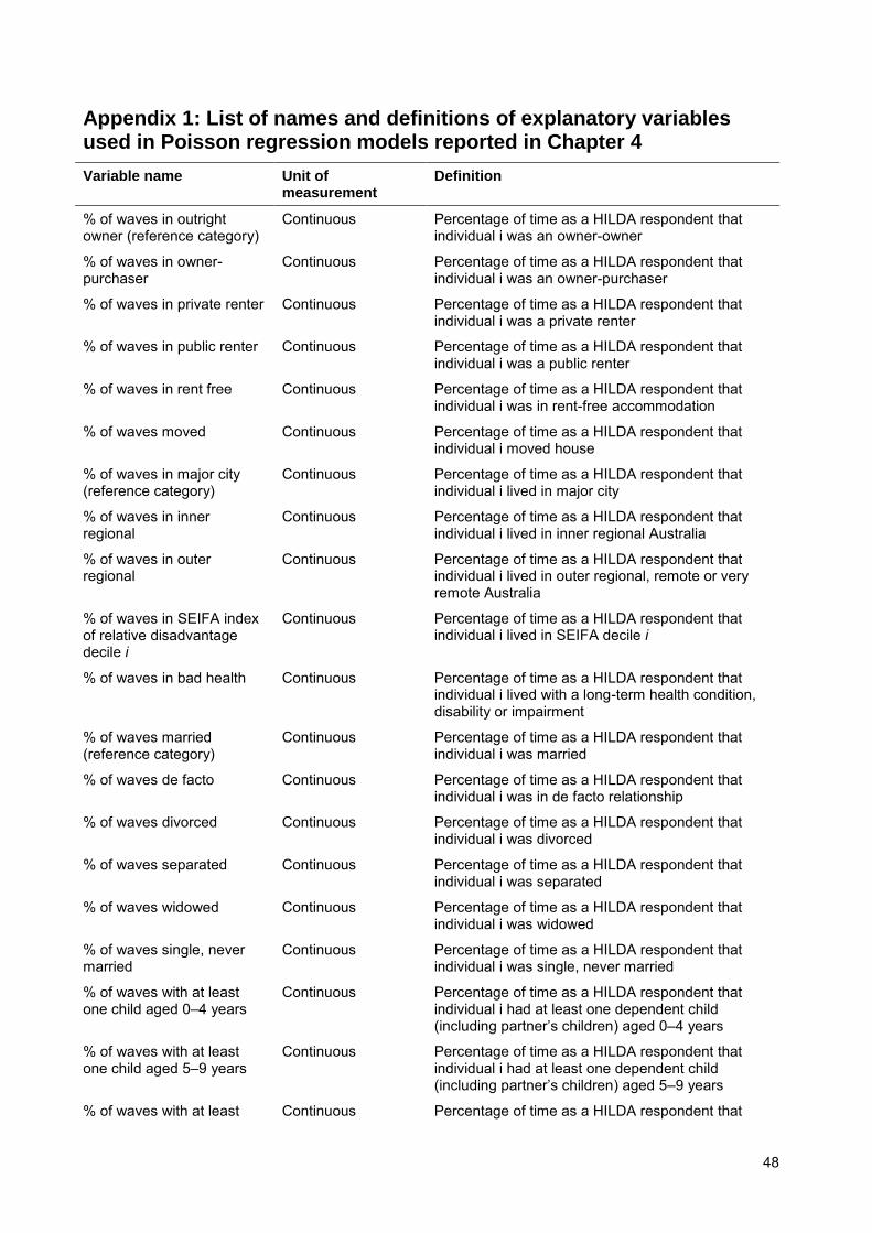
48

Appendix 1: List of names and definitions of explanatory variables used in Poisson regression models reported in Chapter 4

Variable name Unit of measurement

Definition

% of waves in outright owner (reference category)

Continuous Percentage of time as a HILDA respondent that individual i was an owner-owner

% of waves in owner-purchaser

Continuous Percentage of time as a HILDA respondent that individual i was an owner-purchaser

% of waves in private renter Continuous Percentage of time as a HILDA respondent that individual i was a private renter

% of waves in public renter Continuous Percentage of time as a HILDA respondent that individual i was a public renter

% of waves in rent free Continuous Percentage of time as a HILDA respondent that individual i was in rent-free accommodation

% of waves moved Continuous Percentage of time as a HILDA respondent that individual i moved house

% of waves in major city (reference category)

Continuous Percentage of time as a HILDA respondent that individual i lived in major city

% of waves in inner regional

Continuous Percentage of time as a HILDA respondent that individual i lived in inner regional Australia

% of waves in outer regional

Continuous Percentage of time as a HILDA respondent that individual i lived in outer regional, remote or very remote Australia

% of waves in SEIFA index of relative disadvantage decile i

Continuous Percentage of time as a HILDA respondent that individual i lived in SEIFA decile i

% of waves in bad health Continuous Percentage of time as a HILDA respondent that individual i lived with a long-term health condition, disability or impairment

% of waves married (reference category)

Continuous Percentage of time as a HILDA respondent that individual i was married

% of waves de facto Continuous Percentage of time as a HILDA respondent that individual i was in de facto relationship

% of waves divorced Continuous Percentage of time as a HILDA respondent that individual i was divorced

% of waves separated Continuous Percentage of time as a HILDA respondent that individual i was separated

% of waves widowed Continuous Percentage of time as a HILDA respondent that individual i was widowed

% of waves single, never married

Continuous Percentage of time as a HILDA respondent that individual i was single, never married

% of waves with at least one child aged 0–4 years

Continuous Percentage of time as a HILDA respondent that individual i had at least one dependent child (including partner’s children) aged 0–4 years

% of waves with at least one child aged 5–9 years

Continuous Percentage of time as a HILDA respondent that individual i had at least one dependent child (including partner’s children) aged 5–9 years

% of waves with at least Continuous Percentage of time as a HILDA respondent that

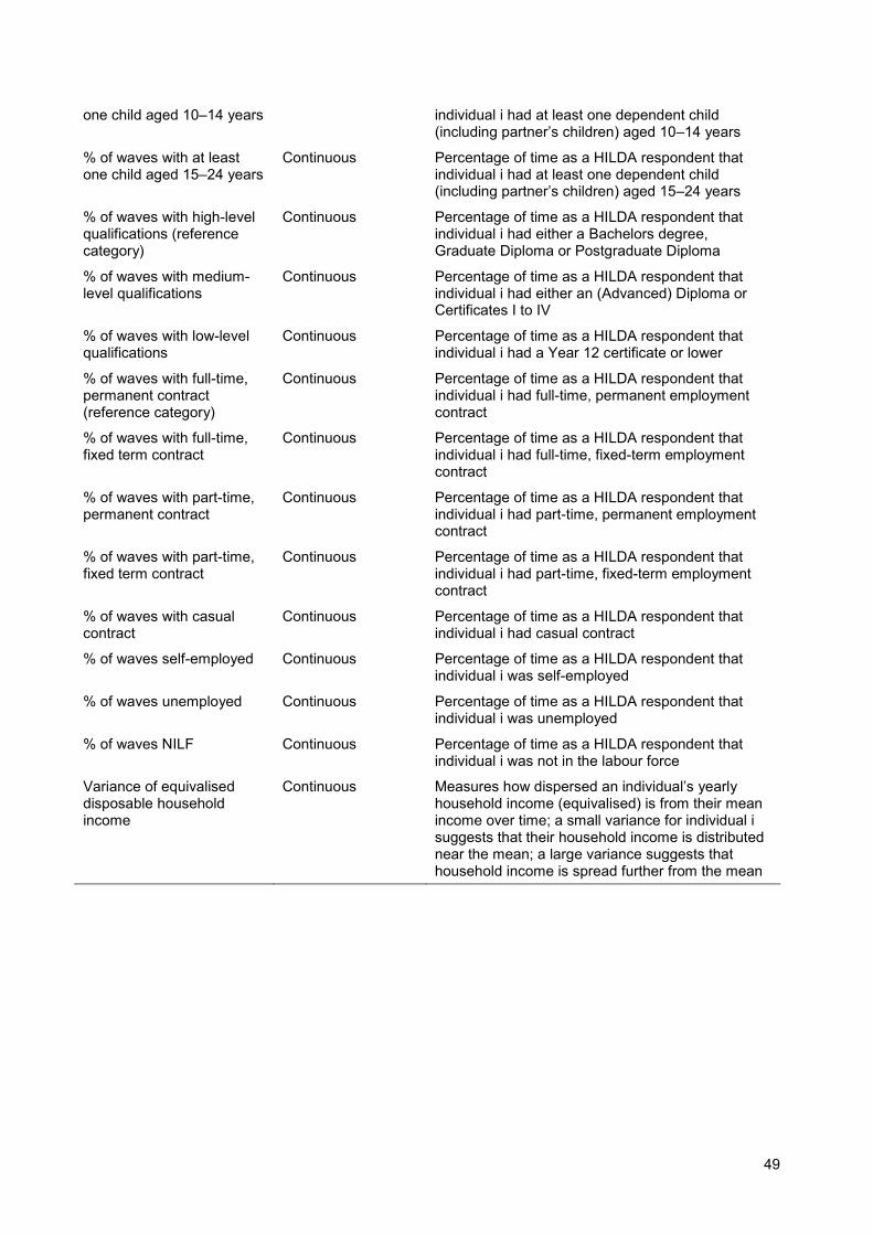
49

one child aged 10–14 years individual i had at least one dependent child (including partner’s children) aged 10–14 years

% of waves with at least one child aged 15–24 years

Continuous Percentage of time as a HILDA respondent that individual i had at least one dependent child (including partner’s children) aged 15–24 years

% of waves with high-level qualifications (reference category)

Continuous Percentage of time as a HILDA respondent that individual i had either a Bachelors degree, Graduate Diploma or Postgraduate Diploma

% of waves with medium-level qualifications

Continuous Percentage of time as a HILDA respondent that individual i had either an (Advanced) Diploma or Certificates I to IV

% of waves with low-level qualifications

Continuous Percentage of time as a HILDA respondent that individual i had a Year 12 certificate or lower

% of waves with full-time, permanent contract (reference category)

Continuous Percentage of time as a HILDA respondent that individual i had full-time, permanent employment contract

% of waves with full-time, fixed term contract

Continuous Percentage of time as a HILDA respondent that individual i had full-time, fixed-term employment contract

% of waves with part-time, permanent contract

Continuous Percentage of time as a HILDA respondent that individual i had part-time, permanent employment contract

% of waves with part-time, fixed term contract

Continuous Percentage of time as a HILDA respondent that individual i had part-time, fixed-term employment contract

% of waves with casual contract

Continuous Percentage of time as a HILDA respondent that individual i had casual contract

% of waves self-employed Continuous Percentage of time as a HILDA respondent that individual i was self-employed

% of waves unemployed Continuous Percentage of time as a HILDA respondent that individual i was unemployed

% of waves NILF Continuous Percentage of time as a HILDA respondent that individual i was not in the labour force

Variance of equivalised disposable household income

Continuous Measures how dispersed an individual’s yearly household income (equivalised) is from their mean income over time; a small variance for individual i suggests that their household income is distributed near the mean; a large variance suggests that household income is spread further from the mean

AHURI Research Centres

AHURI Research Centre—Curtin University

AHURI Research Centre—RMIT University

AHURI Research Centre—Swinburne University of Technology

AHURI Research Centre—The University of Adelaide

AHURI Research Centre—The University of New South Wales

AHURI Research Centre—The University of Sydney

AHURI Research Centre—The University of Tasmania

AHURI Research Centre—The University of Western Australia

Australian Housing and Urban Research Institute

Level 1, 114 Flinders Street, Melbourne Victoria 3000

Phone +61 3 9660 2300

Email information@ahuri.edu.au Web www.ahuri.edu.au