
Factors Affecting the Working Hours of Child Laborers in Dagupan City,...
46
Review of Integrative Business and Economics Research, Vol. 5, no. 4, pp.203-248, October 2016 203 Copyright 2016 GMP Press and Printing (http://buscompress.com/journal-home.html) ISSN: 2304-1013 (Online); 2304-1269 (CDROM); 2414-6722 (Print) Factors Affecting the Working Hours of Child Laborers in Dagupan City, Philippines Michel Danica B. Ong* University of Santo Tomas Lyanne Mae M. Quismundo University of Santo Tomas Valerie Marie V. Sobrepeña University of Santo Tomas Ronald B. Paguta, MAE University of Santo Tomas ABSTRACT Drawing on the survey conducted to 134 respondents gathered through snowball sampling, this study examines the factors that affect the working hours of child laborers (5-17years old) in the pantalan (Filipino term for fish port) of Dagupan City, Pangasinan, Philippines. The data gathered were processed through the Ordinary Least-Squares (OLS) method and were cured using the Weighted Least-Squares (WLS) due to the presence of heteroskedasticity. Results show that the average hours worked by a child laborer in a week is 28 hours. Also, 83 out of 134 respondents are male. Among the explanatory variables, household expenses, household size, gender, schooling, and child’s wage appeared to be statistically significant and affect the variation in the length of time a child works per week with beta coefficients of 0.002, 1.33, -3.1, -0.54, and -0.074 respectively. On the contrary, parental income and child’s age are shown to be statistically insignificant. Keywords: Child labor, parental income, schooling, child’s wage 1. INTRODUCTION Throughout the years, the population of working children has been constantly proliferating especially in the developing countries. The new estimates of International Labour Organization (ILO) as of 2013 indicate that 168 million children worldwide are in child labor, accounting for almost 11 per cent of the child population as a whole. In the case of the Philippines, child labor increased by 30% from 2001 to 2011 with 4.2 million and 5.5 million population respectively. Based on the preliminary results of the 2011 survey on children of the National Statistics Office, 5.492 million children were working, and out of this number, 58.4 percent or an estimated 3.210 million were considered in child labor. A report from Philippine Statistics Authority on survey of children also showed that the estimated 9 percent of child laborers worked for more than 8 hours a day. The case of child labor in the Philippines is not new anymore. However, only a few
-
Upload
nguyennguyet -
Category
Documents
-
view
217 -
download
0
Transcript of Factors Affecting the Working Hours of Child Laborers in Dagupan City,...

Review of Integrative Business and Economics Research, Vol. 5, no. 4, pp.203-248, October 2016 203
Copyright 2016 GMP Press and Printing (http://buscompress.com/journal-home.html) ISSN: 2304-1013 (Online); 2304-1269 (CDROM); 2414-6722 (Print)
Factors Affecting the Working Hours of Child Laborers in Dagupan City, Philippines
Michel Danica B. Ong* University of Santo Tomas Lyanne Mae M. Quismundo University of Santo Tomas Valerie Marie V. Sobrepeña University of Santo Tomas Ronald B. Paguta, MAE University of Santo Tomas
ABSTRACT Drawing on the survey conducted to 134 respondents gathered through snowball sampling, this study examines the factors that affect the working hours of child laborers (5-17years old) in the pantalan (Filipino term for fish port) of Dagupan City, Pangasinan, Philippines. The data gathered were processed through the Ordinary Least-Squares (OLS) method and were cured using the Weighted Least-Squares (WLS) due to the presence of heteroskedasticity. Results show that the average hours worked by a child laborer in a week is 28 hours. Also, 83 out of 134 respondents are male. Among the explanatory variables, household expenses, household size, gender, schooling, and child’s wage appeared to be statistically significant and affect the variation in the length of time a child works per week with beta coefficients of 0.002, 1.33, -3.1, -0.54, and -0.074 respectively. On the contrary, parental income and child’s age are shown to be statistically insignificant. Keywords: Child labor, parental income, schooling, child’s wage 1. INTRODUCTION Throughout the years, the population of working children has been constantly proliferating especially in the developing countries. The new estimates of International Labour Organization (ILO) as of 2013 indicate that 168 million children worldwide are in child labor, accounting for almost 11 per cent of the child population as a whole. In the case of the Philippines, child labor increased by 30% from 2001 to 2011 with 4.2 million and 5.5 million population respectively. Based on the preliminary results of the 2011 survey on children of the National Statistics Office, 5.492 million children were working, and out of this number, 58.4 percent or an estimated 3.210 million were considered in child labor. A report from Philippine Statistics Authority on survey of children also showed that the estimated 9 percent of child laborers worked for more than 8 hours a day. The case of child labor in the Philippines is not new anymore. However, only a few

Review of Integrative Business and Economics Research, Vol. 5, no. 4, pp.203-248, October 2016 204
Copyright 2016 GMP Press and Printing (http://buscompress.com/journal-home.html) ISSN: 2304-1013 (Online); 2304-1269 (CDROM); 2414-6722 (Print)
number of research papers have been made integrating the number of working hours as its measure. On that account, it is of paramount importance to study the reasons beyond what is shown in the numerical figures – what influences the child laborers to work for longer hours. Child labor is always associated with poverty and poor implementation of government policies. Many studies have considered pointing out the macroeconomic factors which cause children to work. Rarely are household decisions examined by researchers of child labor. Countries like the United States of America and Canada have abundant and reliable data about working children. In addition, some developed countries in North America also consider child labor as a legal act. In the Philippines, on the other hand, child labor is not permissible as stated in the Republic Act 7610: Protection of Children Against Child Abuse, Exploitation and Discrimination. With this, data for child labor are very minute which limit further studies about this economic problem. Due to lack of data for child labor, this study hopes to highlight the components that influence child labor at the household level by using primary data. In this way, the world of child laborers can comprehensively be explored. Considering that child labor is a worldwide phenomenon and cannot be eliminated, this study presents the underlying reasons why a child work for long hours and consequently, may be used in consideration in taking actions to lessen the overall time spent by children in working. In order to expose the factors affecting the length of time child laborers spend working, this paper makes use the Dagupan City pantalan (Filipino term for fish port) in the province of Pangasinan as the locus of the study. Dagupan City pantalan is among the top producers of milkfish in the province. From 2001-2003, Dagupan's milkfish production totalled 35,560.1 metric tons (MT), contributing 16.8 percent to the total provincial production. Being a top producer of milkfish, the prevalence of child labor in the area cannot be denied as children can normally be seen working in the pantalan. Based on the Philippine Statistics Authority Census on Population and Housing, as of the year 2010, Dagupan City is the second most populated city in Pangasinan next to San Carlos. It ranks first in terms of the number of households in Pangasinan. The household population by age group is highest on the bracket of 5 to 9, 10 to 14, and 15 to 19 years old. Children aging from 5 to 17 years old, which is the subject of the study, fall within these age brackets. In addition, according to PhilStar news article by De Leon (2002), there is a prevalent incidence of child labor in the Ilocos Region (Region I) especially in the Tobacco-producing provinces where children as early as 10 or 12 years old are already exposed to work hazards. Also, Nathaniel Lacambra, Department of Labor and Employment (DOLE) assistant regional director for Region I, said that during their operations in 2001, 11 child workers in a Kropeck factory, 3 workers in a bakery, and about 15 child workers in a ricemill all in Tayug town, Pangasinan were rescued. Moreover, since Dagupan City is known with prevalence of child labor, DOLE took action in reducing child laborers through providing livelihood assistance to 25 families from different barangays with children who are at risk as child laborers (Sunday Punch, 2013). Help from the Kabuhayan para sa Magulang ng Batang Manggagawa or KASAMA project was also given to provide economic activities to parents of child laborers so they can support the needs of their children. According to Grace Ursua, director of DOLE Ilocos, “It helps to eliminate or lessen child labor incidences by

Review of Integrative Business and Economics Research, Vol. 5, no. 4, pp.203-248, October 2016 205
Copyright 2016 GMP Press and Printing (http://buscompress.com/journal-home.html) ISSN: 2304-1013 (Online); 2304-1269 (CDROM); 2414-6722 (Print)
providing parents or guardians of child laborers or children at risk, access to livelihood opportunities.” By examining the case of Dagupan City, this paper determines the following: 1) Is there a possibility that as the household size augments, the longer the working hours of a child laborer will be? 2) Is there a trade-off between child labor and schooling? Is the number of hours a child laborer devotes to working affected by the number of hours the child spends in school? 3) Does child labor tend to be ‘gender sensitive’, that being a female reduces the number of working hours of a child laborer? 4) Does the age of the child affect the amount of time spent working? 5) What is the impact of parental income on the number of working hours a child spends per week? 6) Is there a correlation between the expenses of the household and the length of time that the child works? and 7) Does the wage received by the child significantly and positively contribute to the household decision of making the child work longer? 2. LITERATURE REVIEW 2.1 Child Labor The International Labour Organization (ILO) 2010 report shows that 306 million children in the world are employed. Among those children, 215 million children are proclaimed as child laborers, in which 115 million children are compelled to work in hazardous work conditions. Child labor is seen by Elijah and Okoruwa (2006) as any work that is detriment to a child, either mentally, physically, socially or morally. It is characterized by the denial of the right of children to proper education and other opportunities. Since it poses economic and social consequences, many studies have been made regarding the macroeconomic causes of the existence of child labor for the purpose of addressing the problem. According to Villamil (2002), in order to get a closer look on child labor in the Philippines, not only macro determinants should be taken into consideration; micro determinants through households must also be observed. In attempt to test the relationship between child labor and household factors, Khanam (2006) used a multinomial logit model to estimate simultaneously the determinants of ‘work’, ‘study’, combining both, or doing neither and found that the household decisions leads to child labor through the number of hours supplied which adversely affects the child’s schooling. Similarly, Phoumin and Fukui (2006) used a stratified and two stages sampling techniques on 12,000 households and 600 units and applied a probit model in Cambodia. Their findings entail a positive relationship between parent decision and hours of work by children. In trying to examine the influence of household decision on child labor, primary surveys are usually utilized. According to Grootaert and Patrinos (2002), one of the main difficulties in furthering the empirical analysis of the determinants of child labor is the dearth or inadequacy of national household surveys that include questions on the labor market participation of both adults and children in the household. Most labor force surveys use a minimum age cut-off of 14 or 15 years, so by definition, most official labor force statistics exclude child labor. This age cut-off is a matter of national practice on the measurement of the economically active population. Because of this data deficiency in labor force surveys, multipurpose household surveys are often said a better source of data

Review of Integrative Business and Economics Research, Vol. 5, no. 4, pp.203-248, October 2016 206
Copyright 2016 GMP Press and Printing (http://buscompress.com/journal-home.html) ISSN: 2304-1013 (Online); 2304-1269 (CDROM); 2414-6722 (Print)
on child labor. Such surveys include a variety of questions on the socioeconomic conditions of the household and often include employment questions with a lower age cut-off than is customary in labor force surveys. The comparative study of Grootaert and Patrinos on the determinants of child labor in Côte d’Ivoire, Colombia, Bolivia and the Philippines focused on the supply-side factors at the household level such as the characteristics of the child, the characteristics of the parents, socioeconomic characteristics of the household, the cost of schooling, and location. Likewise, Alfa (2012) used a primary cross-sectional data set that was sourced from Niger State through the use of survey questionnaires. The questionnaires were directed to the household head and the child between the age of 5 and 14 years in the three headquarters of the three Senatorial zones of the state mainly Bida, Chanchaga and Kontagora. Also through primary survey, Togunde and Richardson (2006) interviewed 1535 parents and children to examine the relationship between child labor and various household variables in urban Nigeria where child labor studies have been very limited. Studies on child labor conducted through primary surveys commonly observe the number of hours child laborers allot in working. The length of time spent on work by a child is treated as the dependent variable since it is a good indicator of the intensity of child labor (G. Haile and B. Haile, 2012). The longer the work hours, the shorter will be the time available for other activities. Alongside, number of hours of work per day was used as the measure for children’s work by Togunde and Richardson (2006). Their findings show that children’s average hours of work range from 2 to 6 hours per day. Phoumin and Fukui (2006) also estimated work hours and the likelihood of school attendance for Cambodian children using simultaneous tobit and probit, respectively. They decided to use hours of child work as the dependent variables since there is considerable variation in hours, thus, making this preferable to estimating participation equations. They found a positive (negative) association between household income and the likelihood of school attendance (work hours). Similarly, Webbink, Smits and Jong (2011) analyzed the data using multilevel regression models with hours spent during the past week (seven days) on household and market work as the dependent variable for the reason that it can reflect the behavior of child laborers best. 2.2 Household Size In relating household size and child labor, a number of studies have found significant and positive effect of household size on children’s working hours. Children from larger households are more likely to work for longer hours to support the members of the family (Fors, 2007; Emerson and Souza, 2008; Aderinto, 2009; Aslam, Awan, and Waqas, 2011; Alfa, 2012). Fors (2007) found that majority of child laborers came from household with 7.4 members and an additional member in the household increases the children’s work hours by 0.16. Similarly, the results of Aslam, Awan, and Waqas (2011) showed that for each increase in household size, there is a corresponding increase in the probability of child labor by 2%. Alfa (2012) also conducted a primary survey of households with working children between 5 and 14 years old as the sampling frame of the study. The study showed the determinants of child labor proxied by hours of labor supplied per day through a logistic regression model. Likewise, results displayed that children with most hours of labor came from households that possess 7 to 9 members, followed by those with

Review of Integrative Business and Economics Research, Vol. 5, no. 4, pp.203-248, October 2016 207
Copyright 2016 GMP Press and Printing (http://buscompress.com/journal-home.html) ISSN: 2304-1013 (Online); 2304-1269 (CDROM); 2414-6722 (Print)
4 to 6 members. Meanwhile, Aderinto (2009) used information on the number of siblings the child laborer has and revealed that majority of the sample came from homes where there were five or more siblings. Based from the results, these studies have concluded that the likelihood that children are involved in long hours of housework or market work increases with the number of siblings and household members, because there are more mouths to feed, more work to be done at home, and higher schooling costs to be paid. Also, children coming from bigger household sizes are educated while others are put to work because they are seen partly as economic investment goods, in that, there is expected return (income) in form of child employment and the provision of financial support for parents (Brown et. al., 2001 as cited in Alfa, 2012). This idea can be supported by the study of Khan (2003) wherein the econometric results showed that larger household size reduces the propensity to go to school. One additional member of the household reduces the likelihood of schooling of children by 5.3 percent. It also reduces the likelihood of combining school and work by 2.1 percent. On the other hand, an incremental change in the household size increases work probability by 1.7 percent for market work, and 7.2 percent for domestic work. Similarly, Filho (2008) showed that the presence of one child aged 0-4 and 5-9 increases boys’ labor participation by 1.9 and 1.4 percentage points respectively. Moreover, boys’ and girls’ labor participation are even higher when they are the oldest child in the household by 5.2 and 2.9 percentage points respectively. Contrastingly, Dada (2013), in testing the null hypothesis that there is no significant relationship between family size and street hawking among children, ended with rejecting the hypothesis and found that child laborers’ hours initially increases with household size and eventually decreases as the size reaches 11-15. The results showed that 61% and 18% of child workers have family sizes of 6-10 and 1-5, respectively. Whereas, 11%, 7%, and 3% have family sizes of 11-15, 16-20, and 26-30, respectively. Similar with Dada (2013), Togunde and Richardson (2006) showed that child laborers with most working hours came from household with 5-9 members and eventually decline as the household size reaches 10 and beyond. With this, both studies have arrived at a conclusion that household size has to do with the welfare of the family. The larger the size of the household relatively to the income of that family, the more is the inadequacy of the welfare and care of such family members, thus higher hours of work for children. However, if the family size is smaller compared with the income, the better will be the welfare and care for the members of such family. On the other hand, the study of G. Haile and B. Haile (2012) has a different finding. Having the length of time spent on work as the dependent variable, household size was shown to have an indeterminate impact a priori on the child’s hours of work. Ceteris paribus, large family size reduces wealth per capita and makes the competition over scarce resources stiffer, which may in turn increase child labor to generate resources to sustain family members. On the other hand, it may be that large family size provides children (at least some of them) with greater opportunity for school attendance and/or fewer work hours, especially if there is specialization among family members. Similarly, Sakellariou and Lall (2000), in analyzing the supply-side socioeconomic determinants of child labor in the Philippines through sequential probit model, used data from the National Household Survey, as well as the Labour Force Survey of the Philippines. The results showed that household size has no effect on the probability of child labor. However,

Review of Integrative Business and Economics Research, Vol. 5, no. 4, pp.203-248, October 2016 208
Copyright 2016 GMP Press and Printing (http://buscompress.com/journal-home.html) ISSN: 2304-1013 (Online); 2304-1269 (CDROM); 2414-6722 (Print)
household size with 4 or less members increases the probability of working for a family enterprise by 4.8%. Despite this relationship, working for a family enterprise does not comprise the definition of child labor. Thus, both studies denied any significant link nor did it provide evidence of a strong positive association between child labor hours and the number of members living in the household. On a different perspective, using hours worked of children in the past 7 days as the dependent variable, Fafchamps and Wahba (2004) through tobit estimator, Phoumin and Fukui (2006) also through tobit and probit, Webbink, Smits and De Jong (2011) through multilevel regression or hierarchical linear model, all found evidence that children in larger households work less. Fafchamps and Wahba regarded the result as consistent with the existence of returns to scale in household. Phoumin and Fukui discovered that household size has positive impact on enrolment and reduce hours worked of children, which means that increasing household size, especially the adults workforce leads to ease the hours worked of children. Webbink, Smits and De Jong stated that Asian children are less involved in work if extended family members are living in the household because it means more helping hands, which allows for a division of tasks at home. This may lead to more time for school for every child and less work. In addition, the work of Bhalotra and Heady (2003) ended with the household size having a marginal effect of -0.54 on the hours worked by children, concluding there is a negative relationship between the two. Consistent with the argument that having more members in the household reduces the probability of child working, Khanam (2008), in his multinomial logit estimates for child labor, proved that the number of total member in the household indeed raises the probability that a school-age child will “study only” relative to the probability that the child will “work only” or “work and study”. This also suggests the inverse relationship between household size and child labor hours which can be seen in the results, “total household members” having a coefficient of -0.11 to the probability of working only. Since a larger household has many potential workers, the probability that any single child will be working is somewhat lower. However, it was also shown that an increase in the number of pre-school children (aged 0-4) reduces the likelihood of full-time schooling and indicates more work hours since schooling will be part-time with work. The effect of the presence of pre-school children on the probability of combining study with work is large for girls but it has no impact on boys which, therefore, indicates that pre-school children generate housework that is particularly done by the girls. In that case, schooling of girls becomes part time instead of fulltime. The study explained that the additional number of pre-school children tends to withdraw school-age children from schooling to work by the increased demand for child care time or by the increased cost of raising pre-school children. H1. The bigger the household size, the longer the working hours of child laborers. 2.3 Schooling The theory of individual labor supply shows that there can be a trade-off between schooling and child labor based on the work-leisure model. In the work-leisure model, any unpaid activity is considered as leisure, so as education. More hours of leisure implies

Review of Integrative Business and Economics Research, Vol. 5, no. 4, pp.203-248, October 2016 209
Copyright 2016 GMP Press and Printing (http://buscompress.com/journal-home.html) ISSN: 2304-1013 (Online); 2304-1269 (CDROM); 2414-6722 (Print)
fewer hours of work. In other words, more hours allocated to school attendance tend to decrease the number of working hours of child laborers. School attendance or education can also be viewed as the human capital formation. Baland and Robison (2000) made a particularly direct connection of human capital formation to child labor when evaluating the efficiency characteristics of household decisions. In relating school attendance with child labor, a detailed survey data from Nepal was used by Fafchamps and Wahba (2004) and the findings of the study show that children residing near the urban areas attend school more and work less in general, but they are more likely to be inclined in market or wage work. On the other hand, children residing in the rural areas attend school less and work more because they are engaged in farm work and supply constraint of schools is present. This is consistent with the fact that there is a better supply of schools and a larger demand for education in the urban areas due to a higher return on education in non-farm activities. Differences on the schooling and child labor relationship on the urban and rural areas were also shown in the study of Villamil (2002). The researcher used sequential probit model and data from the 1995 Child Labor Survey (CLS) of the National Statistics Office (NSO) and the 1998 Annual Poverty Indicator Survey (APIS) data set. In Villamil’s work, being in the National Capital Region (NCR) where public schools are more numerous and more accessible increases the probability that a child will attend school and not work by about 10 percentage points, decreases the probability that a child will study and work at the same time by 20 percentage points, and decreases the probability that a child will work and leave school by 6.4 percentage points. This suggests that eliminating the obstacles that poor households face in sending children to school can effectively reduce child labor. In the work of Ahmed (2012), the latest round of the Multiple Indicator Cluster Survey (MICS) for 2007/08 was used, with a working sample that consists of children between 5 and 14 years of age. To estimate the incidence of child labor and enrolment in Punjab, Pakistan, the study used school enrolment to measure the rate of school attendance. The findings show that public school enrolment can be used as a substitute for child labor ― 1 percentage point increase in enrolment ratio reduces the number of hours of paid child labor by 5 percentage points. The trade-off happens on male child laborers in the urban areas. Meanwhile, Khan (2003), with the use of sequential probit model found that each additional year of education of the child decreases the probability to work by 4.2 percent, concluding that work is the flip side of schooling. Also, Alfa (2012), in trying to examine the relationship between child labor and schooling in three zones of Niger state, used logistic regression model and showed that schooling affects child labor negatively. The descriptive results reveal that out of 399 respondents from each zone, 178(44.61%), 134(33.58%) and 144(36.09%) respectively did not engage in an economic activity simply because they came from household that value education or may be too young to partake in economic activities. Those within the supply of 2 to 5 hours are those that both work and attend school, while the remaining class that engages in pure child labor has a minimum of 6 hours of work. The studies suggest that schooling can be used effectively to reduce child labor because of its positive spillover effects in the form of fewer child labor activities.

Review of Integrative Business and Economics Research, Vol. 5, no. 4, pp.203-248, October 2016 210
Copyright 2016 GMP Press and Printing (http://buscompress.com/journal-home.html) ISSN: 2304-1013 (Online); 2304-1269 (CDROM); 2414-6722 (Print)
In addition, according to Sakellariou & Lall (2000), children who attend school may be drawn away from the labor market.Using data from the National Household Survey and the Labour Force Survey of the Philippines, and a sequential probit model which assumes that household decisions are made in a hierarchical manner, the researchers found out that for any particular household, a child’s time is allocated between schooling, domestic production and income-earning work in the market. This suggests that work is more common among children who have less education and are not attending school. This can be supported by the study of Manda, et al. (2005) which used data from the International Labour Organization and found out that most children who both attend school and work are working for less than 25 hours per week, while children who do not attend school are working for more than 41 hours per week. The study, therefore, also concluded that schooling and child labor participation are negatively correlated. Using the survey data from rural Ethiopia, Haile, G. and Haile, B. (2012) estimated the bivariate probit and the age-adjusted educational attainment equations of male and female children separately. The findings show that there is a prevalent trade-off between schooling and child labor. The practice of combining school and domestic work is 36% points higher for female children while combining school and market work is 24% points higher for male children. This suggests that there is a gender bias even in the combination of school attendance and child labor on male and female child laborers. Similarly, Kis-Katos (2007) said that work and schooling are close substitutes that might also be combined, and offer valuable insights on the nature of the child labor–schooling trade–off. Furthermore, child work and schooling are directly conflicting alternatives where the shorter the length of time the child spends in school, the longer it is that the child is at work. Through the use of trivariate probit regressions, the findings of Kis-Katos (2007) showed that the estimated correlation coefficient between the domestic work and schooling of girls amounts to -0.90, while -0.84 for market work and schooling of boys. However, Ravallion and Wodon (2000) as cited by Ahmed (2012), argues that there is not necessarily a one-to-one relationship between hours worked and school attendance. In Bangladesh, increase in school attendance may result from the child’s leisure time. Therefore, even when educational incentives increase school attendance, they do not necessarily reduce child labor since imposition of school attendance does not generally reduce child labor because forcing children to go to school without changing the economic environment is difficult to enforce and may be counterproductive. Similarly, Kondylis and Manacorda (2012), in making a study on child labor and school attendance in Tanzania, predicted that school attendance may displace child labor in Tanzania. However, findings show that increased probability of school attendance has no significant effect on child labor because most Tanzanian children are employed inside the home and they are likely to combine work with school; but the total working hours of the child becomes less. Also, in Africa, where child labor incidence is highest, a large proportion of its children population are neither in school nor in work, suggesting that increased school attendance might not translate into lower child labor. Alongside, Priyambada, Suryahadi, and Sumarto (2005) used Sakernas and UNICEF’s 100 Village Survey and argued that child labor and schooling are compatible. It is because there are
Review of Integrative Business and Economics Research, Vol. 5, no. 4, pp.203-248, October 2016 211
Copyright 2016 GMP Press and Printing (http://buscompress.com/journal-home.html) ISSN: 2304-1013 (Online); 2304-1269 (CDROM); 2414-6722 (Print)
cases in India that the work load in school is so light that child laborers are able to stay in school in full school hours without seriously affecting the number of hours they spend at work. It is often cited in economic literature that improving educational facilities and providing subsidies to education will increase the possibility that a child will attend school more and work less. Yet another study explaining that school attendance would not lower the case of child labor is the work of Chaudhuri (2004). Considering a model of a small open dual economy which is divided into two informal sectors and one formal sector, the findings of the study show that educational policies do foster a growth in school attendance. However, implementing educational policies simultaneously with liberalized trade and investment policies produced an incompatible effect on the incidence of child labor. In other words, the mutually opposite effects of the three policies had nullified each other so child labor had not gone a significant reduction. On the contrary, in the work of Phoumin and Fukui (2006), since hours supplied are censored at zero hours and depend on the enrolment status of each individual child, the researchers used simultaneous tobit and probit to find the determinants of work hours supplied and enrolment of children. In the study, the decision of schooling and working are simultaneous, and the hours worked by children depend on their enrolment status. The findings show that older children up to 14 years of age tend to work more hours for economic activity if they are attending school because they use their income to pay for school and help their family directly. This indicates that child labor (except the worse form of child labor) is rather increase human capital formation of the child in developing economy like Cambodia. The result can be explained by the Edmonds (2005) who stated that increase in school attendance does not necessarily translate into declines in child labor since the positive impact of increased financial resources on education may outweigh the negative impact of reduced time of study. This finding is consistent with previous studies, for instance, Ray and Lancaster (2004). On the other hand, the work of Grigoli and Sbrana (2012) states that older children do work more but they attend school less. In other cases like of Deb and Rosati (2004), children are idle because reasonable work opportunities do not exist and, at the same time, parents do not send them to school either because of a lack of resources or a high relative price of education. The findings of the study are as follows: 1) In their data for Ghana, 78 percent of children are in school, less than 8 percent work and 14 percent are idle. 2) In their data for India, 64 per cent of children are in school, 13 percent work and 23 percent are idle. 3) In Ghana, 0.66 percent of children in the sample are both working and attending school. 4) Lastly, in India, 0.71 percent of children are both working and attending school. H2. Child laborers who devote more hours in school have shorter number of working hours. 2.4 Age and Gender of the Child Previous studies have shown that child characteristics especially age and gender have an

Review of Integrative Business and Economics Research, Vol. 5, no. 4, pp.203-248, October 2016 212
Copyright 2016 GMP Press and Printing (http://buscompress.com/journal-home.html) ISSN: 2304-1013 (Online); 2304-1269 (CDROM); 2414-6722 (Print)
impact to child labor. Most findings show that the working hours of child laborers increases together with the child’s age. Moreover, males, based on data, constitute the larger population of the child laborers (Sakellariou and Lall, 2000; Kimhi, 2007; Webbink, Smits and Jong, 2012). Furthermore, Becker’s expanded work-leisure model states that household members should allocate their time in which they have a comparative advantage – empirically, females have a comparative advantage in domestic work, which means they are more productive within the household, while males have comparative advantage in market work, which means that they are able to earn more compared with females. In testing the comparative advantage on child workers, Togunde and Richardson (2006) focused on the number of working hours of child laborers. The study was made through drawing interviews on parents and their children. Findings of the study show that female children work more hours. Also, child’s age is significantly and positively correlated with children’s hours of work with a correlation of 8.9; child laborers with most hours of work belong to ages 10-14 years old. The same findings regarding age were on the work of Bhalotra and Heady (2003), except that the gender bias is on the male side. The researchers concluded that males and older children work longer, where for every additional year of child’s age, there is an increase of 2.33 working hours on a Ghana male child laborer, while only 0.46 hours for Pakistan girls. On the contrary, Fors (2007) showed that the gender composition of children has little or no relationship with children’s hours of work. Relating age and gender to child labor, Haile, G. and Haile, B. (2012) used the survey data from rural Ethiopia and revealed the significant relationship of age and gender with the working hours of child laborers. In the study, around 77% of Ethiopian children aged 4–15 in their sample have already started working before turning 8 years old. The study also shows that 1) totaling the hours worked from market and domestic work, child laborers are reported to spend 38 hours a week, on average, with no substantial difference between males and females; and 2) there is a high variation in work hours between male and female children in market and domestic activities – male children work in longer hours (34.7 hours a week) on market work than female (25.3 hours a week), while female children work in longer hours (28.2 hours a week) on domestic work than male (17.2 h a week). This led them to conclude that ‘specialization’ in child labor occurs, supporting Becker’s comparative advantage ― males on market work and females on domestic work. Also guided by Becker’s Allocation of Time, Manda, et al. (2005) used data from the International Labour Organization and showed the age composition of children workers by gender – children in the age group of 10 to 14 years old are more involved in child labor compared to those in the age group of 6 to 9 years old. In both age groups, it is observable that boys are more engaged in labor than girls. Also, among the 6.6 percent of children who are working in domestic services, girls constitute over three-quarters in private households. On the other hand, boys are more economically active in traditional services such as fishing, manufacturing, and quarrying. Having the same conclusion, Goulart and Bedi (2006) used a probit model in examining the effect of the number of hours worked by children. The result indicated that male children are more likely to be economic workers and less likely to be involved in domestic work. It was revealed that

Review of Integrative Business and Economics Research, Vol. 5, no. 4, pp.203-248, October 2016 213
Copyright 2016 GMP Press and Printing (http://buscompress.com/journal-home.html) ISSN: 2304-1013 (Online); 2304-1269 (CDROM); 2414-6722 (Print)
being a male child increases the probability of being an economic worker by 1.2 to 1.8 percentage points while reducing the probability of doing domestic work by 2.5 to 2.7 percentage points. Applying it in the Philippine setting, Villamil (2002) found that in both rural and urban areas, the time allotted for working of both male and female child workers increases with age. Child workers from 5 to 6 years old work on average of 2.7 days and 6 hours a week while child workers from 12 to 14 years old work 3 and a half days and an average of 16.2 hours a week. Also, his findings show that there is a gender and work disparity on the children’s working hours. Males are more likely to engage in market work (14.2 hours a week) than females (13.5 hours a week) and they are also more inclined to farm work because they are assumed to be physically stronger. On the other hand, females are more inclined in urban-based economic activities (9.9 hours a week) such as in trade, manufacturing, and personal and domestic services than males (8.2 hours a week). The study of Fafchamps and Wahba (2004) also found that older girls work more than boys, thus the predisposition to work increases with age in all work categories. For market work, the increase is strongest among children age 14 and above. Like other researchers, Fafchamps and Wahba also concluded that there is strong gender difference associated with child labor – boys engage themselves in market work while girls only engage in subsistence work and household chores; and that as the age of the child increases, the child laborer is more likely to be inclined in longer working hours. With a different reason, Alfa (2012) said that the gender of a child is negatively significant at 10% because female children are easily submissive to the wills of their parents’ decision than their male counterparts in terms of employment participation. This study is in line with the findings of Sakurai (2006) which shows that many female children already are prone to domestic chores than their male equivalents. Another study showing that female child laborers work longer than their male counterparts is that of Phoumin and Fukui (2006). The findings show that females work longer than males in urban areas with working hours of 12.99 hours and 11.83 hours respectively. This is because more males are being enrolled in school. In addition, the data show that as the age of the child increases, the number of working hours also increases. A child whose age is 5 years old work for 1.9 hours a week, and when the child reaches the age of 14, the working hours increased to 27.47 hours a week. In line with this, Khanam (2006) used a multinomial logit model to investigate the relationship between the child’s age and gender, and child labor. Considering children aged 5–17 years old living in rural households of Bangladesh, the study showed that although the gender coefficient has no effect on the probability of working and on the probability that a child will neither study nor work, it has a significant effect on the probability of combining study and work. Female children are more likely to combine study with work, since the odds of combining study with work for girls are nearly 3 times as high as those of boys. This result is not surprising, as the present analysis includes housework in the definition of work. Meanwhile, age coefficient is found to be significant for all categories (“work and study”, “neither” and “work”). The probability of “working” and “combining work and study” increases with age as opposed to the probability of study

Review of Integrative Business and Economics Research, Vol. 5, no. 4, pp.203-248, October 2016 214
Copyright 2016 GMP Press and Printing (http://buscompress.com/journal-home.html) ISSN: 2304-1013 (Online); 2304-1269 (CDROM); 2414-6722 (Print)
only. The researchers’ explanation of this result is that as children grow up, their opportunity cost for study (only) increases, therefore, they either combine study and work or fully specialize in work. H3. Male child laborers work longer than female child laborers. H4. Working hours of child laborers increase together with their age. 2.5 Parental Income Child labor is always associated with poverty or low income. The household production theory of Becker shows how parents maximize household wealth. But in cases where the wealth cannot be maximized due to low income, the household is more likely to resort to having children work to support for the family’s welfare. Due to observable data showing that child labor is prevalent in areas with high poverty incidence, almost all of the studies on child labor used income and tried to test the relationship between the two. One is that of Togunde and Richardson (2006) which showed that majority of child laborers came from households with monthly income below 20,000 Naria, and that as household income increases, the incidence of child labor correspondingly declines. Another is that of G.Haile and B. Haile (2012). With the use of bivariate probit and tobit model with censored regressor, the study found that unemployed parents and parents involved in economic activities who do not generate enough resources are more likely to let their children engage in various activities both within and outside the household to make ends meet. Having unemployed parents increases the probability for a child to work by 7.4 percent. In addition, the results of the Ordinary Least Squares method for the structural estimates on the study of Filho (2008) showed that an additional increase of R$100 in the income of parents reduces the probability of having “worked in the reference week” by 6.3 percentage points for boys and about zero for girls. Also, Ali, Rafi and Aslam (2012) developed questionnaire in order to identify the factors that push child towards work. Based on the data gathered, 49.3 percent are working because their parents sent them to work due to poverty and financial constraints. Parents need children’s income when the resources and opportunities available to them are not sufficient to allow them to meet subsistence needs (Sakellariou and Lall, 2000; Villamil, 2002; Ali and Khan, 2004; Phoumin and Fukui, 2006; Fors, 2007; Chiwaula, 2009; Barman, 2011; Aslam, Awan, and Waqas, 2011). The sequential probit results of Sakellariou and Lall (2000) for the child labor in the Philippines showed that for a household head with income in the lowest quintile, the overall probability of child working increases by about 5%, while 8% in rural areas and 3% in urban areas. Meanwhile, the econometric results of Villamil (2002) from the 1995 NSO Survey in the Philippines suggest that belonging to a poor household that earns less than Php 3,000 a month on average (lowest income quintile) decreases the probability that a child will go to school and not work by 7.5 percentage points, while it increases the probability that a child will drop out of school to work by 4.8 percentage points. Phoumin and Fukui (2006), in taking the logarithm of household income, found that its coefficient on the enrolment status and hours worked by children per week is 0.22 and -1.21, respectively, which lead
Review of Integrative Business and Economics Research, Vol. 5, no. 4, pp.203-248, October 2016 215
Copyright 2016 GMP Press and Printing (http://buscompress.com/journal-home.html) ISSN: 2304-1013 (Online); 2304-1269 (CDROM); 2414-6722 (Print)
to the conclusion that parental income plays a significant role in increasing the probability of child’s enrolment and reducing the hours worked of the child. Fors’ (2007) findings also show that child laborers with most hours of work are with low parental income of below10,000 INR. Similarly, Aslam, Awan, and Waqas (2011) in identifying the supply side determinants of child labour, related monthly income in rupees with the probability of child working. The study showed that low level of parental income drives children into hazardous labour, and majority of these child laborers have parents that are unemployed or underemployed, desperate for secure employment and income. On the basis of the results, the researchers gave policy options to the government on providing employment opportunities for the adult members of families whose survival depends upon the earnings of the children. These studies suggest that the lack of parental resources increases the probability of a child working, confirming the luxury axiom. Basu and Van (1998, p. 416) define the luxury axiom as “parents will send the children to the labor market only if their income from non-child-labor sources drops very low”. On one hand, Beegle, Dehejia, and Gatti (2006) used panel data from Tanzania and found that households respond to transitory income shocks by increasing child labor, both probability and hours worked, but that the extent to which child labor is used as a buffer is lower when households have access to credit. These findings contribute to the empirical literature on the income hypothesis by showing that credit-constrained and lower-income households actively use child labor to smooth their income. Grootaert and Patrinos (2002) found the same results regarding parents’ and households’ poverty status, suggesting that constraints on the poor (to borrow, to insure) increase the odds of child labor. Since poor families are unable to borrow or insure against income shocks, they are more reliant on children’s labor for their survival. Moreover, the findings show that at 90% confidence level, being in the poorest quintile, the probability of making the child work and not attend school is 16.80. On the other hand, according to Rogers and Swinnerton (2004), in the presence of two-sided altruism, i.e., when parents and children care about each other’s utility, increases in parental income need not always lead to increases in school time and to decreases in child labor time. This surprising result derives from the systematic way capital market constraints bind as parental income rises: child labor increases as soon as parental income rises by enough to eliminate transfers from children to parents. The paper identified a surprising property of the BR (Baland and Robinson) model: in the presence of two-sided altruism, some households with higher incomes will send their children to school for fewer hours, and to work for more hours, than households with lower incomes. That low parental income is a proximate cause of child labor is an idea that is almost universally accepted in both the theoretical literature on child labor and in more policy-oriented work. However, household-level empirical studies often fail to find an inverse link between household incomes and child labor. The results of Rogers and Swinnerton may offer a reason why: the relationship between child labor and parental income may be neither continuous nor monotonically decreasing. Similarly, Alfa (2012) found that household welfare measured by dollars earned per day is positively but insignificantly related to household decision and child labor, suggesting that household income does not influence their decision because children participation in labor market is mostly common in the region.

Review of Integrative Business and Economics Research, Vol. 5, no. 4, pp.203-248, October 2016 216
Copyright 2016 GMP Press and Printing (http://buscompress.com/journal-home.html) ISSN: 2304-1013 (Online); 2304-1269 (CDROM); 2414-6722 (Print)
H5. Low parental income leads to higher number of hours worked by child laborers. 2.6 Household Expenses Very few literatures have directly related and used household expenditure as a determinant of the child’s length of time spent on work. Some studies, like those of Lima, Mesquitay, and Wanamaker (2014) and Boutin (2012), only used household expenditure as a proxy for establishing the relationship between wealth or income and hours of work of children. Boutin (2012), with the use of Gaussian kernel regression and nested logit estimation of the supply of child labor (7-14 years old) in rural Mali, found that an increase in the household expenditure decreases child labor probability outside the household by 0.58, thereby concluding a negative relationship between the two. Studies relating household expenditure to the hours worked by child laborers include the work of Bhalotra and Heady (2003). By applying the general equilibrium model, the study showed that in Pakistan, an increase in consumption expenditure of 10% is associated with a reduction in the probability of child’s work by 5 percentage points. Also, conditional on working, the same change in expenditure is expected to reduce hours of work by 1.2 per week (average hours are 15 per week). The corresponding effects for girls in Ghana are 2 percentage points and 0.3 hours per week. Like previous studies, they concluded that there is an inverse relationship between children’s hours of work and household expenditure. In addition, two estimation methods are employed by Priyambada, et. al (2005) to see what affects child labor decisions, the probit and iv-probit model. Households that have at least one child aged five to fourteen years old were interviewed. The study showed that with the use of probit model, the estimation of household expenditure coefficient is -0.0038, while with the use IV-Probit model, the estimation is -0.0219. Both methods that were utilized showed that there is an inverse relationship between household expenditure and households’ decision of sending their children to work. Similarly, according to Dar, et al. (2004), a unit increase in household expenditure reduces the likelihood of child labor by 5 percent. Among urban children, the relationship is even more striking – the marginal impact of one unit increase in logged expenditure on the probability of child working is negative 35 percent. Meanwhile, Guarcello, Mealli and Rosati (2009) followed a probabilistic survey design, covering 7,276 households (3,852 rural and 3,424 urban) with a very high response rate. Result showed that household expenditure reduces child labor and increases full time school attendance. Having the same findings, Edmonds (2004) who used data from the Vietnam Living Standards Surveys (VLSS), explained that child labor declines in households throughout the increasing per capita expenditure distribution because of improvements in economic status. Per capita expenditure improvements, according to Edmonds, can explain 80 percent of the observed decline in child labor for households that emerge from poverty between 1993 and 1998. In addition, Krolikowski (2007), after instrumenting for household expenditure, stated in his study that 1 percent higher household expenditure leads to a 0.21 percent decrease in the probability that any one child in the household
Review of Integrative Business and Economics Research, Vol. 5, no. 4, pp.203-248, October 2016 217
Copyright 2016 GMP Press and Printing (http://buscompress.com/journal-home.html) ISSN: 2304-1013 (Online); 2304-1269 (CDROM); 2414-6722 (Print)
works. Comparably, Blunch, et al. (2002) applied a multi-logit model and found that a 1 percentage point increase in per capita expenditure will lead to a decrease in the probability of engaging in child labor by 2 percent, ceteris paribus. Moreover, Hien (2012) observed that child laborers with total living household expenditure of 420,000 and below work for an average of 11.16 hours per week. Whereas, those with expenditures above 420,000 only work for 9 hours per week. Results showed that child workers with lower household expenditures tend to work longer hours. Contrastingly, using the 2001 Philippine Survey on Children and the level of monthly expenditure as a proxy variable for the household’s fixed assets, Albada, Lanzona, and Tamangan (2004) analyzed through probit model and found that monthly household expenditure is significantly and positively correlated with child work with a coefficient of 0.14. The results indicate that the families with more fixed assets or expenses tend to have more children working. On the other hand, Chiwaula (2009), by solving the derivative of consumption level, opined that consumption expenditure has a negative significant effect on the probability that a child from high consumption households would work in at least one activity, while the same was not significant among the low consumption level households. Chiwaula (2009), therefore, concluded that household expenditure is insignificant to child labor on some levels of household. This is in line with the study of Chamarbagwala and Tchernis (2010) which also showed that household expenditure has no correlation with child labor. H6. The higher the household expenditure, the shorter the time spent by child laborers in working. 2.7 Wage of the Child Using child’s income per week, Togunde and Richardson (2006), through a two stage stratified random sampling technique, showed that 53.6% of the 1,535 respondents work longer hours if the income is above 2,000 Nigerian Naria Currency per week. In addition to this, Murad and Kalam (2013), through a logistic regression model developed by using the data gathered from slum areas, found that child’s own wage rate or income largely and positively increases the likelihood of child working longer since it can be considered as a ‘pull’ factor. With this, Rammohan (2000) recommended that a reduction of child wage rate along with compensation for household could be an effective measure to diminish child labor. In the Philippines, according to Villamil (2002), the places of work that gives the highest mean gross incomes per week to child laborers (market: P1080, mines/construction site: P1051, employer/other persons house: P977), are also the places of work with the most mean days and most mean hours of work per week, 3.7 days and 15.6 hours, 4.4 days and 30.9 hours, 4.4 days and 27.1 hours, respectively. Other places with low wages or income for child laborers also have lower hours of work. Based on Villamil’s findings, the higher the wage rate of the child, the longer hours he devotes to working. Same with Sugawara (2009), even by applying a two-period overlapping generations

Review of Integrative Business and Economics Research, Vol. 5, no. 4, pp.203-248, October 2016 218
Copyright 2016 GMP Press and Printing (http://buscompress.com/journal-home.html) ISSN: 2304-1013 (Online); 2304-1269 (CDROM); 2414-6722 (Print)
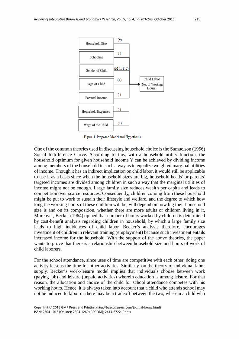
model, the study showed that in poor economies, parents force children to work since income (wage) of the children is crucially the basis of parents’ income. Accordingly, high wage rate for the child also causes parents to decide to have more children. Similarly, using the Ordinary Least Squares method, Kulsoom (2007) found that child’s income is positively related to longer weekly working hours of a child. In the study, the results show that majority, 57.33% of the 150 working children surveyed earns less than 1000 Rupees and work less than the 42.67% that earns greater than or equal to 1000 Rupees. Also considering the impact of child’s wage, Rosenzweig and Evenson (1978) found that the average wage of the sampled children performing wage work in the Philippines is 21.5 pesos, which is two-thirds of the male adult wage rate. Given the relative numbers of hours worked, the finding suggests that, on average, the contribution of a 14-year-old to family income is almost 25 percent of that contributed by the head of the household. This shows how big the contribution of a child’s wage to the family, resulting in the large possibility to push them to work more (longer hours). Additionally, Khan and Ejaz (2001), as cited in Awan, Waqas and Aslam (2011), tried to analyze the supply side determinants of female children by using the primary data in Multan. The study found that children whose wages were 50 to 130 rupees per week work for 6-12 hours, while those with lower wages also work fewer hours. Also, Kimhi (2007) and Kim and Zepeta (2004) used Ordinary Least Squares Method for each of their studies. The results of Kimhi and Zepeta (2004) show that the effect of the shadow wage of children on hours worked are strongly positive at 95% confidence level. Kimhi (2007) also found that for every unit increase in the wage of the child, the length of time spent on work by a child also increases by 0.71 hours. Also trying to get the estimates, Ray (2000) discovered that child’s wage is positively but weakly related to the probability of child labor. Boys’ wages have a coefficient of 0.0016, while girls’ have a coefficient of 0.00164. On the contrary, Bharadwaj and Lakdawala (2013) found with the use of general equilibrium framework/model, that despite of the fall in child’s wage relative to adult wages after the ban from Child Labor Act of 1986 in India, poor families send out more children into the workforce. Also, in the investigation of Dacuycuy and Bayudan-Dacuycuy (2013), the results from the application of Ordinary Least Squares Method showed that wage effect has an estimate of -0.04 to child work. Ersado (2005) had the same result wherein child’s wage falls but child laborers work longer hours. According to him, this is because longer hours are needed in order to accumulate and bring home more money unlike with a high wage. H7. The higher the wage rate of the children, the more hours are worked by child laborers. Conceptual Framework In aiming to test the relationship between household and child characteristics and child labor, the researchers developed a framework in which household size, schooling, gender of child, age of child, parental income, household expenses, and wage of the child are factors that are expected to influence the number of working hours of child laborers.
Review of Integrative Business and Economics Research, Vol. 5, no. 4, pp.203-248, October 2016 219
Copyright 2016 GMP Press and Printing (http://buscompress.com/journal-home.html) ISSN: 2304-1013 (Online); 2304-1269 (CDROM); 2414-6722 (Print)
One of the common theories used in discussing household choice is the Samuelson (1956) Social Indifference Curve. According to this, with a household utility function, the household optimum for given household income Y can be achieved by dividing income among members of the household in such a way as to equalize weighted marginal utilities of income. Though it has an indirect implication on child labor, it would still be applicable to use it as a basis since when the household sizes are big, household heads’ or parents’ targeted incomes are divided among children in such a way that the marginal utilities of income might not be enough. Large family size reduces wealth per capita and leads to competition over scarce resources. Consequently, children coming from these household might be put to work to sustain their lifestyle and welfare, and the degree to which how long the working hours of these children will be, will depend on how big their household size is and on its composition, whether there are more adults or children living in it. Moreover, Becker (1964) opined that number of hours worked by children is determined by cost-benefit analysis regarding children in household, by which a large family size leads to high incidences of child labor. Becker’s analysis therefore, encourages investment of children in relevant training (employment) because such investment entails increased income for the household. With the support of the above theories, the paper wants to prove that there is a relationship between household size and hours of work of child laborers. For the school attendance, since uses of time are competitive with each other, doing one activity lessens the time for other activities. Similarly, on the theory of individual labor supply, Becker’s work-leisure model implies that individuals choose between work (paying job) and leisure (unpaid activities) wherein education is among leisure. For that reason, the allocation and choice of the child for school attendance competes with his working hours. Hence, it is always taken into account that a child who attends school may not be induced to labor or there may be a tradeoff between the two, wherein a child who

Review of Integrative Business and Economics Research, Vol. 5, no. 4, pp.203-248, October 2016 220
Copyright 2016 GMP Press and Printing (http://buscompress.com/journal-home.html) ISSN: 2304-1013 (Online); 2304-1269 (CDROM); 2414-6722 (Print)
attends school may have shorter working hours than a child who does not. In line with this, the study seeks to prove that more hours allocated to schooling tend to decrease the number of working hours of child laborers. Besides the work leisure model, Becker also believes on the principle of comparative advantage. According to him, household members should allocate their time in which they have a comparative advantage or greatest productivity. Moreover, previous studies show that historically, females have a comparative advantage in domestic or household work, while males have comparative advantage in market work. With this, the study would like to reveal whether the principle of comparative advantage also applies even to male and female child laborers. That is, male children tend to work longer than female children. When it comes to age, most findings show that the working hours of child laborers increases together with the child’s age. Furthermore, males, based on data, constitute the larger population of the child laborers. (Kimhi, 2007; Sakellariou and Lall, 2009; Webbink, Smits and Jong, 2012). On one hand, parental income or household income is always the pointed culprit for child labor. In showing whether parental income really influences and affects the working hours of child laborers, the paper will be guided by the household production theory of Gary Becker and the luxury axiom of Basu and Van (1998). The household production theory emphasizes that parents attempt to maximize household wealth. However, in situations where local markets generate significant opportunities to make money when the household is faced with limited resources or resource constraints, the participation of children in such income earning ventures become a mechanism or common strategy for meeting the household’s survival needs and uplifting their present condition. This, in application, will contribute to the probability that a child will engage in work. Similarly, the luxury axiom shows that parents will send the children to the labor market only if the family’s income from non-child labor sources drops very low. Parents send their children to work because they need the children’s income contribution to escape from poverty. Having showed how income might affect the work hours of child laborers, there is a possibility that household expenses might also do, because according to the Keynesian theory of consumption, there is a positive relationship between disposable income and consumption. As income rises, so does total consumer demand on expenditures. This theory can be indirectly related to the number of hours worked by children. Since it is not always the case that the increase in expenditure will be offset by the increase in income, the decision of the household to make a child work for long hours may depend whether the increase in income is greater than the increase in expenditure or vice versa. On the other hand, in using the wage of the child as a factor influencing the decision on how much time should be devoted to working, the work-leisure model of Gary Becker can be used best as the basis since it shows the different effects of wage rate to a person. In its income effect, leisure is treated as a normal good. Higher income implies a desire for more leisure and fewer hours of work. Thus, for a wage increase, income is seen to be raised and so, the income effect lowers the desired hours of work. On the contrary, the substitution effect looks at the higher wage rate as something that raises the relative price of leisure. Thus, for a wage increase, the substitution effect raises the desired work hours.

Review of Integrative Business and Economics Research, Vol. 5, no. 4, pp.203-248, October 2016 221
Copyright 2016 GMP Press and Printing (http://buscompress.com/journal-home.html) ISSN: 2304-1013 (Online); 2304-1269 (CDROM); 2414-6722 (Print)
Another applied theory in the household as the decision making unit is Becker’s Theory of the Allocation of Time (1965). This theory argues that at higher wage rate, income effect increases income and allows household to consume more goods, thereby, decreasing work hours. On the other hand, Becker’s substitution effect shows that higher wage increases hours of work because households substitute. Accordingly, the study wants to find out whether substitution effect or income effect prevails for child laborers. 3. RESEARCH METHOD The study made use of multiple regression analysis specifically Ordinary Least Squares (OLS) method to test the relationship of the factors affecting the variation in the working hours of child laborers and to determine the regression coefficients. Data on the child’s wage per week were divided by the weekly number of hours spent in working to arrive at the wage per hour in order to have a better estimate of the effect of hourly wage to the time a child laborer devotes to work. The initial regression output exhibited heteroskedasticity which led us to use Weighted Least Squares (WLS) method to cure the said error. 3.1 Participants Since the Philippines has only few studies and insufficient and restricted data about child labor, we utilized a primary survey in which questionnaires were sourced from a face-to-face interview to obtain high response rate, in-depth, concise information, and high quality data. The paper examined the case of child labor in the country by employing a case study in the City of Dagupan, Pangasinan with hours of work spent during the past week or the past seven (7) days as the reference period and the pantalan as the main locus. Dagupan City pantalan has been chosen as the locus of the study because it is where children can be seen working. The children are working as fishermen, goods lifters, and fish deboners. The survey was conducted for three days in the city’s pantalan, from June 12 to 14, 2015. The total respondents comprised 172 child workers with the following criteria: (1) aging from 5 to 17 years old; (2) living together with their parents or guardians; (3) earning a wage or working in exchange for payment; and (4) worked during the reference period. Each questionnaire was analyzed and carefully evaluated in order to ensure that the information provided by the respondents were reliable. After the assessment, we arrived with 134 responses. 3.2 Sampling Method The child laborers, which are the subject of the study, are difficult to locate because the respondents are hidden. Such population is hidden because of its illegality in the Philippines. Because of this, we decided to use the snowball sampling which is a non-probability sampling method that can be used to have an access to this kind of population. 3.3 Econometric Model To determine and explore the factors influencing the working hours of child laborers, the specification of the model with the explanatory variables expected to affect child labor is

Review of Integrative Business and Economics Research, Vol. 5, no. 4, pp.203-248, October 2016 222
Copyright 2016 GMP Press and Printing (http://buscompress.com/journal-home.html) ISSN: 2304-1013 (Online); 2304-1269 (CDROM); 2414-6722 (Print)
as follows: WHOURSi = β0 + β1HSIZEi + β2SCHOOLi + β3GENDERi + β4AGEi + β5INCOMEi + β6EXPENSEi + β7CHILD’S WAGEi+ ε wherein WHOURS is child labor measured through the number of working hours in the past 7 days, HSIZE is the number of household members living under one roof, SCHOOL is the number of hours spent in school in the past week, GENDER represents a dummy variable (1 for male and 0 for female child worker), INCOME is the amount of parental income received in the past week, EXPENSE is the amount of household expenditures incurred in the past week, and CHILD’S WAGE is the wage received by the child worker in the past week. The model is derived from Togunde and Richardson (2006). Togunde and Richardson used child labor measured by child’s number of hours of work per day as the dependent variable, and among the independent variables that were included in the study are the size of the household, number of children in the household, age of the child, gender composition of the child, as well as of the household head, child’s income per week, parental education, and household income. Alongside, the model is also derived from the work of Phoumin and Fukui (2006) wherein the determinants of hours supplied by child laborers in Cambodia are being examined. The study has the same explanatory variables with that of Togunde and Richardson, except that Phoumin and Fukui measured the hours of work in the past 7 days, and the study takes into consideration rural-urban classification and school attendance that comes in the form of dummy variables. 3.4 Survey Instrument The researchers used a survey questionnaire derived from the National Child Labor Survey of the International Labor Organization (ILO). The questionnaire contained both open-ended and closed-ended questions. Furthermore, to lessen the possibility of confusion and inaccuracy of response, the survey was conducted through a guided scheme where the researchers asked the questions and transcribed the responses into the questionnaire. The respondents of the survey were the child laborers and their parents or guardians. The first part of the survey, which is the adult questionnaire, was directed to the parents or guardians. This part aims to gather information about the household size, estimated weekly household expenses, and estimated weekly parental income. The respondents (parents or guardian) were asked the total number of persons in the household, the number of children and adults in the household, the number of working adults in the household, the estimated amount of expenses per week, and their estimated income for the past week. The second part of the survey is the child questionnaire which was addressed to the child laborers. The respondents (child laborers) were asked about their age, gender, as well as their status of education, whether attending school or not, and how many hours have they rendered in school to discover if the presence of trade-off between working and schooling exists. The children were also asked the number of hours they spent on working for the past week and their estimated wage for the past week. For the survey to attain consistency

Review of Integrative Business and Economics Research, Vol. 5, no. 4, pp.203-248, October 2016 223
Copyright 2016 GMP Press and Printing (http://buscompress.com/journal-home.html) ISSN: 2304-1013 (Online); 2304-1269 (CDROM); 2414-6722 (Print)
of information, there are certain requirements that must be met by the respondents. For the child laborers, they must be 5 to 17 years old working for an expected income either at home or outside. Those children who earn money through profit-making such as collecting non-biodegradable waste and selling them are not included. For the parents or guardian of the child laborers, there are no specific requirements as long as they are living together with the child laborer. 3.5 Test for Validity In order to test the validity of the said survey form, the researchers conducted a pre-test on Navotas Fish Port Complex on the 18th of April, 2015. Being the premier fish center of the Philippines and one of the largest in Asia, Navotas fish port supplies fish to the largest markets in Metro Manila. According to the Philippine Fisheries Development Authority (PFDA), around 20 commercial fishing vessels unload a total volume of about 800 tons and thousands of buyers visit the port each day. In addition, a business center made up of markets, restaurants, and the like are established outside the main fish port complex. Because of this, the presence of child labor in the Navotas fishing industry cannot be denied. Furthermore, the fish port has been featured in an award-winning documentary of GMA News Brigada episode entitled “Gintong Krudo”. The documentary told the story of three child workers, 11, 12, and 13 years old, who swim in the dirty waters of Navotas to collect crude oil with a sponge. This crude oil can be sold starting at a price of 40 pesos. “Gintong Krudo” has won the “One World Award” in the US Film and Video Festival, and the “Silver World Medal” in the 2014 New York Festival (Sazon, 2014). The data obtained from the pre-test in the field was processed using statistical package for social sciences (SPSS) computer software and resulted to a Cronbach’s alpha of 0.766, suggesting the validity of the questionnaire and that the variables of the study have relatively high internal consistency. 4. RESULTS AND DISCUSSION One of the projects of the Department of Labor and Employment (DOLE) is the Campaign for a Child Labor-Free Barangay which influences change and obtains commitment and support from various stakeholders to make barangays free from child labor. While 54 barangays have been declared by DOLE to be child labor-free in 2014, the project is still initiated to the barangays of Dagupan City which means that child labor is still existent in the area. Barangay Pantal (pantalan) of Dagupan City is not yet declared as child labor-free. Tons of sea products are being unloaded each day at the pantalan of Dagupan with milkfish comprising the largest percent contribution to the total provincial production. Also, having visited the pantalan, we were able to observe that child laborers already became an essential part of their labor population as they can be normally seen working as fishermen, goods lifters, fish deboners, and vendors. Furthermore, Dagupan City is the second most populated city in Pangasinan next to San Carlos as of the year 2010 according to the Philippine Statistics Authority Census on Population and Housing. It ranks first in terms of the number of households in Pangasinan. The household population by age group is highest on the bracket of 5 to 9, 10 to 14, and 15 to 19 years old. Children

Review of Integrative Business and Economics Research, Vol. 5, no. 4, pp.203-248, October 2016 224
Copyright 2016 GMP Press and Printing (http://buscompress.com/journal-home.html) ISSN: 2304-1013 (Online); 2304-1269 (CDROM); 2414-6722 (Print)
aging from 5 to 17 years old, which is the subject of the study, fall within these age brackets.
Table 1: Child laborers based on the number of persons living in the household
Household Size Frequency
1 0
2 10
3 8
4 13
5 16
6 20
7 or more 67
Total 134
Table 2: Child laborers based on the weekly expenses of the household
Household Expenses Frequency
Less than Php 500 12
Php. 501-750 4
Php. 751-1,000 2
Php. 1,001-1,250 3
Php. 1,251- 2,500 65
Php.2,501-3,750 28
Php3,751 and over 20
Total 134
Table 3: Child laborers based on the consolidated weekly income of their parents
Parental Income Frequency Less than Php 770 12
Php. 771-1154 6
Php.1155-1923 33
Php.1924-4808 57
Php.4809 and over 26

Review of Integrative Business and Economics Research, Vol. 5, no. 4, pp.203-248, October 2016 225
Copyright 2016 GMP Press and Printing (http://buscompress.com/journal-home.html) ISSN: 2304-1013 (Online); 2304-1269 (CDROM); 2414-6722 (Print)
Total 134 Considering the information acquired from the first part of the questionnaire, Table 1 shows where do most child laborers belong to in terms of the number of people living together with them under one roof. Given the following choices on the questionnaire, the researchers were able to identify their household sizes. Most of the respondents have household sizes of 7 or more. There are 67 respondents who answered that there are 7 or more members living in the household, which is already 50% of the total sample. Following 7 or more persons is a large percentage of 15% that have households with 6 members. However, none of the 134 respondents answered that they came from a household size of 1 which signifies that there are no child laborers at the pantalan area of Dagupan City that lives alone and working for himself/herself only. This is consistent with other studies that find large household as common characteristic for working children (Fors, 2007; Filho, 2008; Aderinto, 2009; Alfa, 2012). Table 2 presents the number of respondents for each range of the weekly expenses of the household. In the survey conducted, 48.50% of the total respondents (65 households) answered that they spend Php. 1,251- 2,500 weekly to meet the needs and wants of its members. On the other hand, only 1.48% of the total respondents (2 households) have Php. 751-1,000 as their household expenditure for the past week. Table 3 depicts the weekly income of the child laborers’ parents. Given the 5 ranges of weekly income, 57 of the respondents (42.53%) answered that their parents usually earn Php.1924-4808 weekly. Taking into account the international definition of child labor, the researchers have interviewed child workers aging from 5 to 17 years old for the second part of the survey form. Unfortunately, no data were gathered from child laborers aging from 5 to 6 years old as no child with that age was seen working in the pantalan. This may be due to the nature of the job which cannot be executed by children of very young ages. Among the 134 child laborers, 51 are females and 83 are males which represent 38% and 62% of the whole sample respectively (Table 4).
Table 4: Child laborers by age and gender
Age Gender Total
Male Female
5 to 6 0 0 0
7 to 8 2 1 3
9 to 10 4 0 4
11 to 12 9 6 15
13 to 14 37 15 52
15 to 16 21 14 35
17 10 15 25
Total 83 51 134
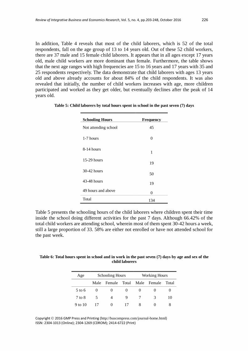
Review of Integrative Business and Economics Research, Vol. 5, no. 4, pp.203-248, October 2016 226
Copyright 2016 GMP Press and Printing (http://buscompress.com/journal-home.html) ISSN: 2304-1013 (Online); 2304-1269 (CDROM); 2414-6722 (Print)
In addition, Table 4 reveals that most of the child laborers, which is 52 of the total respondents, fall on the age group of 13 to 14 years old. Out of these 52 child workers, there are 37 male and 15 female child laborers. It appears that in all ages except 17 years old, male child workers are more dominant than female. Furthermore, the table shows that the next age ranges with high frequencies are 15 to 16 years and 17 years with 35 and 25 respondents respectively. The data demonstrate that child laborers with ages 13 years old and above already accounts for about 84% of the child respondents. It was also revealed that initially, the number of child workers increases with age, more children participated and worked as they get older, but eventually declines after the peak of 14 years old.
Table 5: Child laborers by total hours spent in school in the past seven (7) days
Schooling Hours Frequency
Not attending school 45
1-7 hours 0
8-14 hours 1
15-29 hours 19
30-42 hours 50
43-48 hours 19
49 hours and above 0 Total 134
Table 5 presents the schooling hours of the child laborers where children spent their time inside the school doing different activities for the past 7 days. Although 66.42% of the total child workers are attending school, wherein most of them spent 30-42 hours a week, still a large proportion of 33. 58% are either not enrolled or have not attended school for the past week.
Table 6: Total hours spent in school and in work in the past seven (7) days by age and sex of the
child laborers
Age Schooling Hours Working Hours Male Female Total Male Female Total
5 to 6 0 0 0 0 0 0
7 to 8 5 4 9 7 3 10
9 to 10 17 0 17 8 0 8

Review of Integrative Business and Economics Research, Vol. 5, no. 4, pp.203-248, October 2016 227
Copyright 2016 GMP Press and Printing (http://buscompress.com/journal-home.html) ISSN: 2304-1013 (Online); 2304-1269 (CDROM); 2414-6722 (Print)
Table 6 displays the child laborers’ total hours in their work and school for the past 7 days. Longest school hours are evident from ages 13 to 14 years old where male child laborers have longer school hours than females. It is surprising that despite having the longest time spent in school, children with ages between 13 to 14 years old also exhibited the longest working hours in which males work more hours. It is thus presented that male child laborers have both longer schooling and working hours with 228 and 284 hours respectively. A total of 491 hours is spent for working by all the child respondents. With that, the time spent for working is 137 hours longer than the time spent in school which is only 354 hours a week. This implies that child laborers allot more time on working than attending school. Table 7 reveals the wage being received by the child laborers from their work for the past 7 days. Of the 134 respondents, it can be seen that more than half of the child laborers (74 respondents or 55.22%) receive less than or equal to Php. 700 a week. The number of child workers decline at each level of wage brackets. It is observable that fewer children get to be included in the higher wage brackets. It shows that even though child laborers work for long hours, they are still paid not high enough of their hard work.
Table 7: Child laborers by wage received in the past seven (7) days
Child's Wage Frequency Less than or equal to Php. 700 74
Php. 701-1,200 36 Php.1,201-1,700 11 Php. 1,701-2,200 7 Php. 2,201- 2,700 2 Php.2,701-3,200 2
Php. 3,201 and over 2 Total 134
Table 8: Descriptive Statistics
Mean Std. Deviation N
11 to 12 24 21 45 32 20 52
13 to 14 127 57 184 106 49 155
15 to 16 43 35 78 81 61 142
17 12 9 21 50 74 124 Total hours 228 126 354 284 207 491
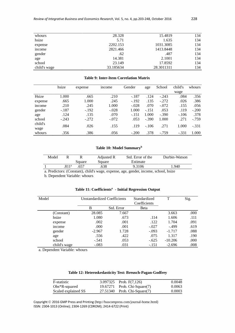
Review of Integrative Business and Economics Research, Vol. 5, no. 4, pp.203-248, October 2016 228
Copyright 2016 GMP Press and Printing (http://buscompress.com/journal-home.html) ISSN: 2304-1013 (Online); 2304-1269 (CDROM); 2414-6722 (Print)
whours 28.328 15.4819 134 hsize 5.71 1.635 134 expense 2202.153 1031.3085 134 income 2821.466 1413.8448 134 gender .62 .487 134 age 14.381 2.1001 134 school 23.149 17.8592 134 child's wage 33.185634 28.3011311 134
Table 9: Inter-Item Correlation Matrix
hsize expense income Gender age School child's
wage whours
Hsize 1.000 .665 .210 -.187 .124 -.243 .084 .356 expense .665 1.000 .245 -.192 .135 -.272 .026 .386 income .210 .245 1.000 -.028 .070 -.072 .155 .056 gender -.187 -.192 -.028 1.000 -.151 .053 .119 -.200 age .124 .135 .070 -.151 1.000 -.390 -.106 .378 school -.243 -.272 -.072 .053 -.390 1.000 .271 -.759 child's wage .084 .026 .155 .119 -.106 .271 1.000 -.331
whours .356 .386 .056 -.200 .378 -.759 -.331 1.000
Table 11: Coefficientsa - Initial Regression Output
Model Unstandardized Coefficients Standardized Coefficients
T Sig.
B Std. Error Beta
(Constant) 28.085 7.667 3.663 .000 hsize 1.080 .673 .114 1.606 .111 expense .002 .001 .122 1.704 .091 income .000 .001 -.027 -.499 .619 gender -2.967 1.728 -.093 -1.717 .088 age .556 .422 .075 1.317 .190 school -.541 .053 -.625 -10.206 .000 child's wage -.083 .031 -.151 -2.696 .008
a. Dependent Variable: whours
Table 12: Heteroskedasticity Test: Breusch-Pagan-Godfrey
F-statistic 3.097325 Prob. F(7,126) 0.0048 Obs*R-squared 19.67271 Prob. Chi-Square(7) 0.0063 Scaled explained SS 27.51340 Prob. Chi-Square(7) 0.0003
Table 10: Model Summaryb
Model R R
Square Adjusted R
Square Std. Error of the
Estimate Durbin-Watson
1 .811a .657 .638 9.3106 1.940 a. Predictors: (Constant), child's wage, expense, age, gender, income, school, hsize b. Dependent Variable: whours
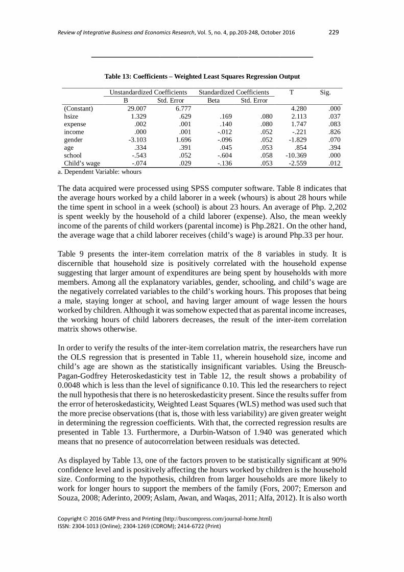
Review of Integrative Business and Economics Research, Vol. 5, no. 4, pp.203-248, October 2016 229
Copyright 2016 GMP Press and Printing (http://buscompress.com/journal-home.html) ISSN: 2304-1013 (Online); 2304-1269 (CDROM); 2414-6722 (Print)
Table 13: Coefficients – Weighted Least Squares Regression Output
Unstandardized Coefficients Standardized Coefficients T Sig. B Std. Error Beta Std. Error
(Constant) 29.007 6.777 4.280 .000 hsize 1.329 .629 .169 .080 2.113 .037 expense .002 .001 .140 .080 1.747 .083 income .000 .001 -.012 .052 -.221 .826 gender -3.103 1.696 -.096 .052 -1.829 .070 age .334 .391 .045 .053 .854 .394 school -.543 .052 -.604 .058 -10.369 .000 Child’s wage -.074 .029 -.136 .053 -2.559 .012
a. Dependent Variable: whours
The data acquired were processed using SPSS computer software. Table 8 indicates that the average hours worked by a child laborer in a week (whours) is about 28 hours while the time spent in school in a week (school) is about 23 hours. An average of Php. 2,202 is spent weekly by the household of a child laborer (expense). Also, the mean weekly income of the parents of child workers (parental income) is Php.2821. On the other hand, the average wage that a child laborer receives (child’s wage) is around Php.33 per hour.
Table 9 presents the inter-item correlation matrix of the 8 variables in study. It is discernible that household size is positively correlated with the household expense suggesting that larger amount of expenditures are being spent by households with more members. Among all the explanatory variables, gender, schooling, and child’s wage are the negatively correlated variables to the child’s working hours. This proposes that being a male, staying longer at school, and having larger amount of wage lessen the hours worked by children. Although it was somehow expected that as parental income increases, the working hours of child laborers decreases, the result of the inter-item correlation matrix shows otherwise. In order to verify the results of the inter-item correlation matrix, the researchers have run the OLS regression that is presented in Table 11, wherein household size, income and child’s age are shown as the statistically insignificant variables. Using the Breusch-Pagan-Godfrey Heteroskedasticity test in Table 12, the result shows a probability of 0.0048 which is less than the level of significance 0.10. This led the researchers to reject the null hypothesis that there is no heteroskedasticity present. Since the results suffer from the error of heteroskedasticity, Weighted Least Squares (WLS) method was used such that the more precise observations (that is, those with less variability) are given greater weight in determining the regression coefficients. With that, the corrected regression results are presented in Table 13. Furthermore, a Durbin-Watson of 1.940 was generated which means that no presence of autocorrelation between residuals was detected. As displayed by Table 13, one of the factors proven to be statistically significant at 90% confidence level and is positively affecting the hours worked by children is the household size. Conforming to the hypothesis, children from larger households are more likely to work for longer hours to support the members of the family (Fors, 2007; Emerson and Souza, 2008; Aderinto, 2009; Aslam, Awan, and Waqas, 2011; Alfa, 2012). It is also worth

Review of Integrative Business and Economics Research, Vol. 5, no. 4, pp.203-248, October 2016 230
Copyright 2016 GMP Press and Printing (http://buscompress.com/journal-home.html) ISSN: 2304-1013 (Online); 2304-1269 (CDROM); 2414-6722 (Print)
noting that household size is also significant even at 5% level of significance which means that the number of people living together in the household is really an essential factor affecting the variation in work hours of the child laborers. The results of the regression output expose that for every additional member in the household, the hours worked by children per week increases by 1.33 hours. Fors (2007) also found that an additional member in the household increases the children’s work hours by 0.16. Although both Fors’ and this study found a direct relationship between the two, the beta coefficient of household size in this study is greater than that of Fors’. A conceivable reason is that, based on the survey, majority of the child workers’ households are comprised of more children rather than working adults. This may explain the larger weight of an increase in the household size for this study since additional members, specifically children, implies that there are more mouths to feed, more work to be done at home, and higher schooling costs to be paid. Whereas, if the household is comprised of more adults, more working and helping hands may lead to more income, division of tasks, opportunity to go to school full time, and less work hours (Fafchamps and Wahba, 2004; Phoumin and Fukui, 2006; Webbink, Smits and De Jong, 2011). Likewise, household expense is also positively correlated with hours of work and is in contrast with what was predicted that the higher the household expenditure, the shorter the time spent by child laborers working. The result shows that as the household from where the child laborer belongs to climbs to a higher range of household expenses, the working hours of the child laborers increase by 0.002 hours per week. Since very few literatures have directly related and used household expenditure as a determinant of the child’s length of time spent on work, many studies have used expenditure as a proxy variable and/or measure of wealth and income like those of Dar, et al. (2004), Priyambada, et. al (2005), Boutin (2012), and Lima, Mesquitay, and Wanamaker (2014). Similarly, Edmonds (2004) explained that child labor declines in households throughout the increasing per capita expenditure distribution because it represents improvements in economic status. These studies have concluded a negative relationship between household expenses and hours worked by children. Since our study has not treated household expenditure as a measure of another, this may explain why the result is not in accordance with the proposition. It can also be deduced that the weekly expenses covering all the members of the household are not offset by the parental income and the income contributed by the other members as well, making the child laborers in the household work in longer hours to supplement the money for the payment of expenditures (Albada, Lanzona, and Tamangan, 2004). Looking at the child’s characteristics, gender, schooling, and child’s wage are all statistically significant and have inverse relationship with the time spent in work. Surprisingly, male child laborers work 3 hours less than female child laborers. It is true that males constitute the larger part of the child labor population in the pantalan as presented by Table 4 and supported by the studies of Sakellariou and Lall (2000), Kimhi (2007), and Webbink, Smits and Jong (2012). However, the result for the child’s gender is found to be inconsistent with the hypothesis of the study wherein male child laborers work for longer hours than females. One possible reason is the nature of the job in the pantalan, female child laborers, along with their mothers mostly engage as fish vendors, deboners, and cleaners of clams and other shellfish which take longer hours, from early

Review of Integrative Business and Economics Research, Vol. 5, no. 4, pp.203-248, October 2016 231
Copyright 2016 GMP Press and Printing (http://buscompress.com/journal-home.html) ISSN: 2304-1013 (Online); 2304-1269 (CDROM); 2414-6722 (Print)
morning to afternoon, compared to male child laborers who mostly have jobs as lifters and catchers of fish which end before lunch after unloading the fishes. The results with regards to this variable can be further supported by the study of Togunde and Richardson (2006) which also made use of interviews with the child laborers and their parents. The findings of their study show that female children work more hours. The same findings were on the work of Alfa (2012) where it is exposed that female children are more submissive to the wills of their parents’ decisions when it comes to engaging in work activities. Furthermore, in the work of Phoumin and Fukui (2006), males work for shorter hours since they are more prioritized to be enrolled in school. It is also very evident that there is indeed a trade-off between child labor and schooling. Every hour devoted by a child in school decreases the time spent in working by about half an hour or 30 minutes. This is consistent with the proposition of the researchers that child laborers who devote more hours in school have shorter number of working hours. Most of the child laborers commit absenteeism in school or cutting of classes in order to work longer hours (Sakellariou and Lall, 2000; Haile, G. and Haile, B., 2012). Also, Manda, et al. (2005) used data from the International Labour Organization, found out that most children who both attend school and work are working for less than 25 hours per week, while children who do not attend school are working for more than 41 hours per week. Likewise, Ahmed’s (2012) results show that for every 1 percentage point increase in enrolment ratio, the number of hours of child labor is reduced by 5 percentage points. The regression results of this study showed evidence for the majority of the studies that conclude that work is the flip side of schooling which includes that of Kis-Katos (2007), “child work and schooling are directly conflicting alternatives where the shorter the length of time the child spends in school, the longer it is that the child is at work.” Moreover, for every peso increase in the hourly wage that a child receives during his work time, he works 0.074 hours or almost 5 minutes less per week. The result shows discordancy when compared to the hypothesis that the higher the wage rate of the children, the more hours are worked by child laborers. A negative relationship between wage and hours worked by children was established (Ersado, 2005; Bharadwaj and Lakdawala, 2013; Bayudan-Dacuycuy, 2013). According to Ersado, children’s wage fall but child laborers work longer hours because longer hours are needed in order to accumulate and bring home more money unlike with a high wage. Using the same rationale, since most of the child laborers in the pantalan receive low wages which is not congenial to the relatively long working hours performed by them, an increase in their wages enable them to afford more leisure since less time is needed to be spent in working in order to earn and bring home money compared with a lower wage. On the other hand, different from the notion that low parental income leads to higher number of hours worked by child laborers, the results showed parental income to be statistically insignificant, which may suggest that although many literatures have proven parental income to be a great factor in the decision of the children to work, it may not influence the hours worked by children the same way. It may be because even though the child’s own parents have high income, it may not be sufficient to cover the overall costs of the large household and meet the needs of all the people living together with them in the house. Since the people living together with them are usually their families too,

Review of Integrative Business and Economics Research, Vol. 5, no. 4, pp.203-248, October 2016 232
Copyright 2016 GMP Press and Printing (http://buscompress.com/journal-home.html) ISSN: 2304-1013 (Online); 2304-1269 (CDROM); 2414-6722 (Print)
nuclear or extended, they decide not only based on their parents’ earnings, but also on the earnings and welfare of the whole household. The regression result is congruent with that of Alfa (2012) which states that household income does not influence the parents’ decision in sending their children to work because children participation in labor market is mostly common in the region. This can be applied to the case of child labor in the pantalan of Dagupan since it is already commonly practiced in their work environment. Contrary to the proposition of a positive relationship between age and child labor, age is also shown to be statistically insignificant as a determining factor when taking hours worked as the predicted variable. Age being insignificant can be supported by the data presented in Table 4, which shows that as the age increases, the population of the child workers also increases but eventually declines when they reach 15 years old and so on. This is approximately when the child enters third year and continues to entering college which may give reason to children to prioritize their school and invest more on education than working. The regression results also suggest that the child’s age when related to working hours may depend on the locus of the study and the nature of the job. Since children working in the pantalan, regardless of their age, have the same set of jobs i.e. they work in almost the same number of hours. 5. CONCLUDING REMARKS The study, in determining the factors influencing the variation in the time spent by children in working, revealed that among the 7 explanatory variables, household size, household expense, child’s gender, schooling, and child’s wage statistically affect the working hours of the child laborers in the pantalan area of City of Dagupan, Pangasinan. Reaffirming the positive effect of household size, an additional member in the household increases the hours worked by children by 1.33 hours per week. Furthermore, as the household from where the child laborer belongs to climbs to a higher range of household expenses, the working hours of the child laborer increase by 0.002 hours per week. Exploring for the child’s characteristics, it was found that male child laborers work less than females with a difference of 3 hours per week. A salient trade-off between the child’s working hours and the time they devote to schooling is also validated as the hours worked decrease by 0.5 hours or 30 minutes per week due to additional hour spent in school. Also shown as a major factor, the child’s wage, in particular, a peso increase in the hourly wage that a child receives, lessens his work time by 0.074 hours or almost 5 minutes per week. On one side, parental income and the age of the child are perceived to be statistically insignificant. Notwithstanding the evidence and conventional results of published literatures, this study denied any significant link or association between these variables and the working hours of child laborers in the case of Dagupan City’s pantalan. Since the prevalence of child labor in the Philippines specifically in the case of Dagupan City pantalan can never be fully eliminated, endeavors must be made in order to lessen the exposure of children to this kind of activity. Indeed, laws are already present and several policies are made by the government in order to gradually diminish child labor in different parts of Pangasinan but the enforcement of these policies seems to be inadequate, and this is further supported by the evidence that child labor practices are present in the pantalan of Dagupan. The laws governing labor in the Philippines duly protect the

Review of Integrative Business and Economics Research, Vol. 5, no. 4, pp.203-248, October 2016 233
Copyright 2016 GMP Press and Printing (http://buscompress.com/journal-home.html) ISSN: 2304-1013 (Online); 2304-1269 (CDROM); 2414-6722 (Print)
children against the risk associated with working in various industries, yet, some businesses remain to be disregarded. Based on the preliminary results of the 2011 survey on children of the National Statistics Office, 62% of the children in hazardous labor were working in the agriculture sector which includes farming and fishing, 30.1% were in the services sector, and the rest (7.6%) worked in the industry sector. Because data shows that child labor is rampant on the agricultural sector, which includes the pantalan surveyed, profuse attention and strict execution of the existing policies must be imposed by the government to the operation of this type of business. Since Barangay Pantal and Barangay II, the barangays composing the pantalan, cannot solely administer and eradicate the severe incidence of child labor, a partnership with the city government of Dagupan should transpire to be able to comprehensively observe how the fishing industry in the area makes use of children as vendors, fishermen, goods lifters, and cleaners of clams and shellfish. In view of the empirical results generated by the study, Barangay Pantal and Barangay II could provide a source of livelihood and create job opportunities for the parents and family members of the child laborers. A stable source of income will be beneficial since it will lessen their vulnerability to fluctuations in earnings and compensate for the high expenditure that draws children to work longer hours. Training and development programs to be offered to the adult members of the household so as to further enhance their skills and abilities will also be useful since it will allow them to maximize the jobs that will be made available to them. It is also discernible that despite the presence of free education offered by public schools, child laborers spend a large amount of time in working. They even commit absenteeism and cutting classes just to work. Considering free education is already accessible and they still choose work over school, establishing more schools, rooms and enhancing facilities may encourage children to go to school in a way, but the effect would only be minimal. Establishing recreational facilities and activities like basketball, volleyball, and other sports in schools near the pantalan may also entice children to spend more time in school than engaging in work for the enjoyment that they experience. Programs and seminars for parents and children should also be conducted by the barangays to enlighten them how the negative effects of child labor will outweigh the immediate yet interim solution for making the child work. This way, both parents and children may be convinced that the children must attend school for the long-term effect of human capital formation rather that attending short-term and low-paying employment. It will also be of great deal if the principals of different schools near the pantalan be included in the seminars in order for them to be well-informed that most of the children studying are engaged in child labor, and consequently, help in taking actions against it. Aside from the cash grants provided to the recipients of the Pantawid Pamilyang Pilipino Program (4Ps), the city government of Dagupan may offer supplementary benefits to help in the finances of families or households that will satisfy the following conditions: (1) eligible recipient of 4Ps (2) has a child or children belonging in a certain age that is/are not involve in both market and domestic work in exchange for payment (3) all the children are attending school. By doing so, not only their money would be enlarge to cover the expenses, children will also have allowance when attending school, be able to buy school
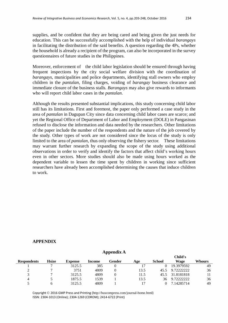
Review of Integrative Business and Economics Research, Vol. 5, no. 4, pp.203-248, October 2016 234
Copyright 2016 GMP Press and Printing (http://buscompress.com/journal-home.html) ISSN: 2304-1013 (Online); 2304-1269 (CDROM); 2414-6722 (Print)
supplies, and be confident that they are being cared and being given the just needs for education. This can be successfully accomplished with the help of individual barangays in facilitating the distribution of the said benefits. A question regarding the 4Ps, whether the household is already a recipient of the program, can also be incorporated in the survey questionnaires of future studies in the Philippines. Moreover, enforcement of the child labor legislation should be ensured through having frequent inspections by the city social welfare division with the coordination of barangays, municipalities and police departments, identifying stall owners who employ children in the pantalan, filing charges, voiding of barangay business clearance and immediate closure of the business stalls. Barangays may also give rewards to informants who will report child labor cases in the pantalan. Although the results presented substantial implications, this study concerning child labor still has its limitations. First and foremost, the paper only performed a case study in the area of pantalan in Dagupan City since data concerning child labor cases are scarce; and yet the Regional Office of Department of Labor and Employment (DOLE) in Pangasinan refused to disclose the information and data needed by the researchers. Other limitations of the paper include the number of the respondents and the nature of the job covered by the study. Other types of work are not considered since the locus of the study is only limited to the area of pantalan, thus only observing the fishery sector. These limitations may warrant further research by expanding the scope of the study using additional observations in order to verify and identify the factors that affect child’s working hours even in other sectors. More studies should also be made using hours worked as the dependent variable to lessen the time spent by children in working since sufficient researchers have already been accomplished determining the causes that induce children to work. APPENDIX
Appendix A
Respondents Hsize Expense Income Gender Age School Child's Wage Whours
1 7 3125.5 385 0 17 0 19.3979592 49 2 7 3751 4809 0 13.5 45.5 9.72222222 36 3 7 3125.5 4809 0 11.5 45.5 31.8181818 11 4 5 1875.5 1539 1 13.5 36 9.72222222 36 5 6 3125.5 4809 1 17 0 7.14285714 49
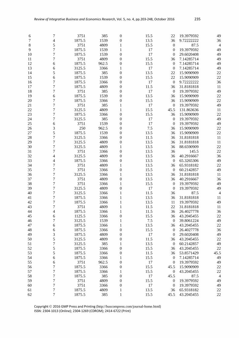
Review of Integrative Business and Economics Research, Vol. 5, no. 4, pp.203-248, October 2016 235
Copyright 2016 GMP Press and Printing (http://buscompress.com/journal-home.html) ISSN: 2304-1013 (Online); 2304-1269 (CDROM); 2414-6722 (Print)
6 7 3751 385 0 15.5 22 19.3979592 49 7 4 1875.5 1539 0 13.5 36 9.72222222 36 8 5 3751 4809 1 15.5 0 87.5 4 9 7 1875.5 1539 1 17 0 19.3979592 49 10 7 1875.5 1539 0 17 0 29.6020408 49 11 7 3751 4809 0 15.5 36 7.14285714 49 12 6 1875.5 962.5 0 15.5 0 7.14285714 49 13 6 3125.5 3366 1 17 0 7.14285714 49 14 5 1875.5 385 0 13.5 22 15.9090909 22 15 6 1875.5 1539 0 15.5 22 15.9090909 22 16 7 1875.5 3366 0 17 0 9.72222222 36 17 7 1875.5 4809 0 11.5 36 31.8181818 11 18 7 3751 385 0 17 0 19.3979592 49 19 6 1875.5 1539 0 13.5 36 15.9090909 22 20 7 1875.5 3366 0 15.5 36 15.9090909 22 21 7 3751 385 1 17 0 19.3979592 49 22 7 3125.5 4809 1 15.5 45.5 131.863636 11 23 7 1875.5 3366 0 15.5 36 15.9090909 22 24 7 3125.5 385 0 17 0 19.3979592 49 25 6 3751 1539 0 17 0 19.3979592 49 26 3 250 962.5 0 7.5 36 15.9090909 22 27 5 1875.5 1539 0 13.5 36 15.9090909 22 28 7 3125.5 3366 0 11.5 36 31.8181818 11 29 7 3125.5 4809 0 13.5 36 31.8181818 11 30 7 3125.5 4809 1 13.5 36 88.6590909 22 31 7 3751 3366 0 13.5 36 145.5 22 32 4 3125.5 4809 0 13.5 36 40.2916667 36 33 4 1875.5 3366 0 13.5 0 65.3265306 49 34 7 3751 4809 1 13.5 36 65.9318182 22 35 7 3751 3366 0 15.5 0 60.2142857 49 36 7 3125.5 3366 1 13.5 36 31.8181818 11 37 7 3751 4809 0 13.5 36 40.2916667 36 38 7 3751 3366 1 15.5 0 19.3979592 49 39 7 3125.5 4809 0 17 0 19.3979592 49 40 7 3125.5 3366 1 11.5 36 87.5 4 41 7 1875.5 3366 1 13.5 36 31.8181818 11 42 7 1875.5 3366 1 13.5 11 19.3979592 49 43 7 3751 4809 1 11.5 22 31.8181818 11 44 4 1875.5 3366 1 11.5 36 26.4027778 36 45 6 1125.5 3366 0 15.5 36 43.2045455 22 46 7 3125.5 1539 1 7.5 0 39.8061224 49 47 6 1875.5 3366 1 13.5 36 43.2045455 22 48 6 1875.5 3366 0 15.5 0 26.4027778 36 49 3 1875.5 4809 0 17 0 29.6020408 49 50 5 3125.5 4809 0 11.5 36 43.2045455 22 51 7 3125.5 385 1 13.5 0 60.2142857 49 52 5 1875.5 3366 0 15.5 36 43.2045455 22 53 5 1875.5 3366 0 11.5 36 53.8571429 45.5 54 6 1875.5 3366 1 15.5 0 7.14285714 49 55 6 3751 962.5 0 17 0 19.3979592 49 56 7 1875.5 3366 0 15.5 45.5 15.9090909 22 57 7 1875.5 3366 1 15.5 0 43.2045455 22 58 7 1875.5 385 0 17 45.5 87.5 4 59 7 3751 4809 0 15.5 0 19.3979592 49 60 7 3751 3366 0 17 0 19.3979592 49 61 7 1875.5 4809 1 13.5 36 65.9318182 22 62 7 1875.5 385 1 15.5 45.5 43.2045455 22

Review of Integrative Business and Economics Research, Vol. 5, no. 4, pp.203-248, October 2016 236
Copyright 2016 GMP Press and Printing (http://buscompress.com/journal-home.html) ISSN: 2304-1013 (Online); 2304-1269 (CDROM); 2414-6722 (Print)
63 7 1875.5 1539 0 15.5 36 43.2045455 22 64 4 875.5 3366 1 17 0 7.14285714 49 65 7 3125.5 1539 1 13.5 45.5 88.6590909 22 66 5 1875.5 1539 1 15.5 36 15.9090909 22 67 7 3125.5 3366 1 15.5 45.5 15.9090909 22 68 7 1875.5 3366 1 13.5 0 19.3979592 49 69 7 3125.5 3366 1 13.5 22 15.9090909 22 70 7 3125.5 1539 1 13.5 22 15.9090909 22 71 7 1875.5 3366 0 15.5 0 19.3979592 49 72 7 1875.5 1539 1 13.5 45.5 15.9090909 22 73 7 3125.5 3366 1 11.5 22 31.8181818 11 74 6 1875.5 1539 1 9.5 22 15.9090909 22 75 7 1875.5 3366 1 11.5 36 31.8181818 11 76 5 1125.5 385 1 11.5 22 15.9090909 22 77 4 1875.5 3366 1 11.5 22 7.14285714 49 78 5 1875.5 962.5 1 15.5 22 9.72222222 36 79 7 1875.5 1539 1 11.5 0 19.3979592 49 80 7 3125.5 3366 1 17 0 19.3979592 49 81 2 625 1539 1 13.5 36 31.8181818 11 82 4 1875.5 3366 0 17 36 31.8181818 11 83 5 1125.5 3366 1 13.5 36 43.2045455 22 84 7 1875.5 3366 1 15.5 22 26.4027778 36 85 7 1875.5 3366 0 11.5 0 29.6020408 49 86 5 3125.5 1539 1 9.5 45.5 31.8181818 11 87 7 1875.5 3366 0 13.5 36 15.9090909 22 88 4 1875.5 385 1 13.5 45.5 31.8181818 11 89 7 3751 4809 1 15.5 36 31.8791209 45.5 90 2 250 1539 1 13.5 36 31.8181818 11 91 6 1875.5 3366 1 15.5 22 15.9090909 22 92 4 1875.5 3366 1 13.5 36 15.9090909 22 93 3 250 1539 1 13.5 36 31.8181818 11 94 2 250 3366 1 13.5 36 31.8181818 11 95 3 250 3366 1 13.5 45.5 31.8181818 11 96 2 250 1539 1 13.5 22 31.8181818 11 97 5 1875.5 4809 0 17 0 26.4027778 36 98 6 3751 3366 1 15.5 0 42.8681319 45.5 99 2 250 1539 1 13.5 22 31.8181818 11 100 2 625 1539 1 13.5 36 31.8181818 11 101 6 1875.5 4809 1 13.5 0 40.2916667 36 102 7 3125.5 1539 0 17 0 7.69230769 45.5 103 6 1875.5 3366 0 13.5 45.5 31.8181818 11 104 6 1875.5 3366 1 17 36 43.2045455 22 105 7 1875.5 1539 0 13.5 45.5 31.8181818 11 106 7 1875.5 3366 1 15.5 0 26.4027778 36 107 3 1875.5 962.5 0 13.5 36 15.9090909 22 108 4 3125.5 4809 1 13.5 0 15.9090909 22 109 4 625 1539 1 9.5 45.5 87.5 4 110 6 875.5 3366 1 17 45.5 222.772727 11 111 6 1875.5 3366 1 15.5 36 43.2045455 22 112 7 1875.5 4809 1 15.5 0 39.8061224 49 113 7 3125.5 3366 1 15.5 0 54.1805556 36 114 7 1875.5 3366 1 7.5 45.5 87.5 4 115 5 1875.5 962.5 1 15.5 22 9.72222222 36 116 7 1875.5 1539 1 11.5 0 19.3979592 49 117 7 3125.5 3366 1 17 0 19.3979592 49 118 2 625 1539 1 13.5 36 31.8181818 11 119 5 3125.5 1539 1 9.5 36 31.8181818 11

Review of Integrative Business and Economics Research, Vol. 5, no. 4, pp.203-248, October 2016 237
Copyright 2016 GMP Press and Printing (http://buscompress.com/journal-home.html) ISSN: 2304-1013 (Online); 2304-1269 (CDROM); 2414-6722 (Print)
120 7 1875.5 3366 0 13.5 22 15.9090909 22 121 4 1875.5 385 1 13.5 36 31.8181818 11 122 7 3751 4809 1 15.5 0 31.8791209 45.5 123 2 250 1539 1 13.5 22 31.8181818 11 124 7 1875.5 3366 1 13.5 0 39.8061224 49 125 7 3751 1539 1 13.5 45.5 31.8181818 11 126 3 1875.5 3366 1 17 22 15.9090909 22 127 7 1875.5 4809 1 15.5 0 26.4027778 36 128 6 1875.5 3366 1 15.5 36 15.9090909 22 129 4 1875.5 3366 1 13.5 36 15.9090909 22 130 3 250 1539 1 13.5 36 31.8181818 11 131 2 250 3366 1 13.5 36 31.8181818 11 132 3 250 3366 1 13.5 36 31.8181818 11 133 2 250 1539 1 13.5 45.5 31.8181818 11 134 5 1875.5 4809 0 17 0 26.4027778 36
Appendix B
Child laborers based on the number of persons living in the household
Household Size Frequency
1 0
2 10
3 8
4 13
5 16
6 20
7 or more 67
Total 134
Appendix C
Child laborers based on the weekly expenses of the household
Household Expenses Frequency
Less than Php 500 12
Php. 501-750 4

Review of Integrative Business and Economics Research, Vol. 5, no. 4, pp.203-248, October 2016 238
Copyright 2016 GMP Press and Printing (http://buscompress.com/journal-home.html) ISSN: 2304-1013 (Online); 2304-1269 (CDROM); 2414-6722 (Print)
Php. 751-1,000 2
Php. 1,001-1,250 3
Php. 1,251- 2,500 65
Php.2,501-3,750 28
Php3,751 and over 20
Total 134
Appendix D
Child laborers based on the consolidated weekly income of their parents
Parental Income Frequency
Less than Php 770 12
Php. 771-1154 6
Php.1155-1923 33
Php.1924-4808 57
Php.4809 and over 26
Total 134
Appendix E
Child laborers by age and gender
Age Gender Total
Male Female
5 to 6 0 0 0

Review of Integrative Business and Economics Research, Vol. 5, no. 4, pp.203-248, October 2016 239
Copyright 2016 GMP Press and Printing (http://buscompress.com/journal-home.html) ISSN: 2304-1013 (Online); 2304-1269 (CDROM); 2414-6722 (Print)
7 to 8 2 1 3
9 to 10 4 0 4
11 to 12 9 6 15
13 to 14 37 15 52
15 to 16 21 14 35
17 10 15 25
Total 83 51 134
Appendix F
Child laborers by total hours spent in school in the past seven (7) days
Schooling Hours Frequency
Not attending school 45
1-7 hours 0
8-14 hours 1
15-29 hours 19
30-42 hours 50
43-48 hours 19
49 hours and above 0
Total 134
Appendix G
Total hours spent in school and in work in the past seven (7) days by age and sex of the child laborers
Age Schooling Hours Working Hours
Male Female Total Male Female Total
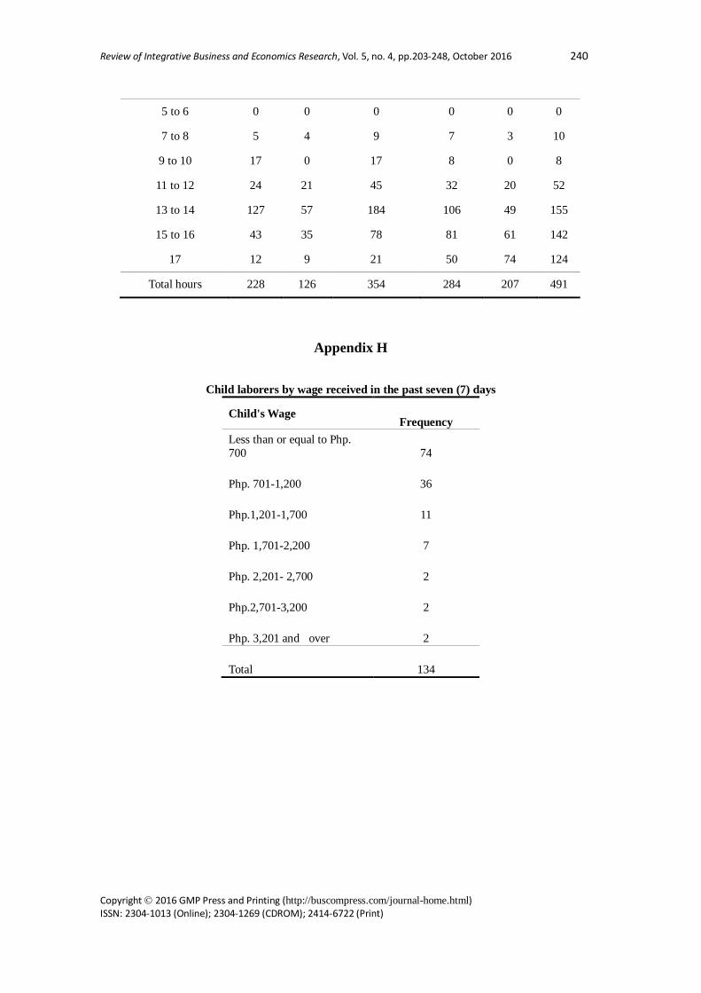
Review of Integrative Business and Economics Research, Vol. 5, no. 4, pp.203-248, October 2016 240
Copyright 2016 GMP Press and Printing (http://buscompress.com/journal-home.html) ISSN: 2304-1013 (Online); 2304-1269 (CDROM); 2414-6722 (Print)
Appendix H
Child laborers by wage received in the past seven (7) days
Child's Wage Frequency
Less than or equal to Php. 700 74
Php. 701-1,200 36
Php.1,201-1,700 11
Php. 1,701-2,200 7
Php. 2,201- 2,700 2
Php.2,701-3,200 2
Php. 3,201 and over 2
Total 134
5 to 6 0 0 0 0 0 0
7 to 8 5 4 9 7 3 10
9 to 10 17 0 17 8 0 8
11 to 12 24 21 45 32 20 52
13 to 14 127 57 184 106 49 155
15 to 16 43 35 78 81 61 142
17 12 9 21 50 74 124
Total hours 228 126 354 284 207 491

Review of Integrative Business and Economics Research, Vol. 5, no. 4, pp.203-248, October 2016 241
Copyright 2016 GMP Press and Printing (http://buscompress.com/journal-home.html) ISSN: 2304-1013 (Online); 2304-1269 (CDROM); 2414-6722 (Print)
Appendix J
Inter-Item Correlation Matrix
hsize expense Income gender age school child's wage
whours
hsize 1.000 .665 .210 -.187 .124 -.243 .084 .356 expense .665 1.000 .245 -.192 .135 -.272 .026 .386 income .210 .245 1.000 -.028 .070 -.072 .155 .056 gender -.187 -.192 -.028 1.000 -.151 .053 .119 -.200 age .124 .135 .070 -.151 1.000 -.390 -.106 .378 school -.243 -.272 -.072 .053 -.390 1.000 .271 -.759 child's wage
.084 .026 .155 .119 -.106 .271 1.000 -.331
whours .356 .386 .056 -.200 .378 -.759 -.331 1.000
Appendix K
Appendix I
Descriptive Statistics Mean Std.
Deviation N
whours 28.328 15.4819 134
hsize 5.71 1.635 134
expense 2202.153 1031.3085 134 income 2821.466 1413.8448 134 gender .62 .487 134 age 14.381 2.1001 134 school 23.149 17.8592 134 child's wage
33.185634 28.3011311 134

Review of Integrative Business and Economics Research, Vol. 5, no. 4, pp.203-248, October 2016 242
Copyright 2016 GMP Press and Printing (http://buscompress.com/journal-home.html) ISSN: 2304-1013 (Online); 2304-1269 (CDROM); 2414-6722 (Print)
Model Summaryb
Model R R Square
Adjusted R Square
Std. Error of the Estimate
Durbin-Watson
1 .811a .657 .638 9.3106 1.940
a. Predictors: (Constant), child's wage, expense, age, gender, income, school, hsize
b. Dependent Variable: whours
Appendix L
Coefficientsa - Initial Regression Output Model Unstandardized Coefficients Standardized
Coefficients t Sig.
B Std. Error Beta
(Constant) 28.085 7.667 3.663 .000 hsize 1.080 .673 .114 1.606 .111 expense .002 .001 .122 1.704 .091 income .000 .001 -.027 -.499 .619 gender -2.967 1.728 -.093 -1.717 .088 age .556 .422 .075 1.317 .190 school -.541 .053 -.625 -10.206 .000 child's wage -.083 .031 -.151 -2.696 .008
a. Dependent Variable: whours
Appendix M

Review of Integrative Business and Economics Research, Vol. 5, no. 4, pp.203-248, October 2016 243
Copyright 2016 GMP Press and Printing (http://buscompress.com/journal-home.html) ISSN: 2304-1013 (Online); 2304-1269 (CDROM); 2414-6722 (Print)
Heteroskedasticity Test: Breusch-Pagan-Godfrey
F-statistic 3.097325 Prob. F(7,126) 0.0048
Obs*R-squared 19.67271 Prob. Chi-Square(7) 0.0063
Scaled explained SS 27.51340 Prob. Chi-Square(7) 0.0003
Appendix N
Coefficients – Weighted Least Squares Regression Output Unstandardized Coefficients Standardized Coefficients t Sig.
B Std. Error Beta Std. Error (Constant) 29.007 6.777 4.280 .000 hsize 1.329 .629 .169 .080 2.113 .037** expense .002 .001 .140 .080 1.747 .083** income .000 .001 -.012 .052 -.221 .826** gender -3.103 1.696 -.096 .052 -1.829 .070** age .334 .391 .045 .053 .854 .394** school -.543 .052 -.604 .058 -10.369 .000** Child’s wage -.074 .029 -.136 .053 -2.559 .012**
Note: Dependent Variable: whours, ** 10% level of significance

Review of Integrative Business and Economics Research, Vol. 5, no. 4, pp.203-248, October 2016 244
Copyright 2016 GMP Press and Printing (http://buscompress.com/journal-home.html) ISSN: 2304-1013 (Online); 2304-1269 (CDROM); 2414-6722 (Print)
Appendix O Reliability Scale: ALL VARIABLES
Case Processing Summary
N %
Cases
Valid 50 100.0
Excludeda 0 .0
Total 50 100.0
a. Listwise deletion based on all variables in the procedure.
Appendix P
Reliability Statistics
Cronbach's Alpha
Cronbach's Alpha Based on
Standardized Items
N of Items
.766 .716 8
Inter-Item Correlation Matrix
Household Size
Household Expenses
Parental Income
Child's Gender
Child's Age
School Attendance
Child's Wage
Child's Working
Hours
Household Size 1.000 .775 .436 .244 .173 .042 .465 .606 Household Expenses .775 1.000 .324 .265 .276 .166 .290 .559 Parental Income .436 .324 1.000 .017 .320 -.076 .410 .380 Child's Gender .244 .265 .017 1.000 .202 .167 -.224 .059 Child's Age .173 .276 .320 .202 1.000 -.022 .187 .312 School Attendance .042 .166 -.076 .167 -.022 1.000 -.089 -.140 Child's Wage .465 .290 .410 -.224 .187 -.089 1.000 .580 Child's Working Hours .606 .559 .380 .059 .312 -.140 .580 1.000

Review of Integrative Business and Economics Research, Vol. 5, no. 4, pp.203-248, October 2016 245
Copyright 2016 GMP Press and Printing (http://buscompress.com/journal-home.html) ISSN: 2304-1013 (Online); 2304-1269 (CDROM); 2414-6722 (Print)
Appendix Q
ACKNOWLEDGEMENT
This research is made possible through the guidance of our God Almighty, the help and the support of the researchers’ family, friends, relatives, and all the people who contributed in the pre-test and final survey conducted at the Navotas City fish port and Dagupan City fish port respectively. We would also like to express our gratitude to our supportive adviser, Mr. Ronald Bag-o Paguta, MAE, who encouraged us to push through with the topic and do primary research despite the difficulty of finding the respondents, and patiently checked the grammar, organization, and format of the paper. We are also grateful to the interviewed families who allotted time to provide information for the completion of this study.
REFERENCES [1] Albada, F., Lanzona, L., & Tamangan, R.. (2004). An Empirical Analysis on the
trade-off between schooling and child labor in the Philippines. Philippine Journal of Development, 31(2), 215-246.
[2] Aderinto, A. (2009). Social correlates and coping measures of street-children: A comparative study of street and non-street children in South-Western Nigeria. Child Abuse & Neglect, 24(9), 1199–1213.
[3] Ahmed, H. (2012). The impact of public school enrolment on child labor in Punjab, Pakistan. The Lahore Journal of Economics, 17(2), 1–34.
[4] Alfa, A.B. (2012). The influence household decision on child labour activities: analysis from rural areas of Niger state, Nigeria. International Journal of Advanced Research in Management and Social Sciences, 1(3), 32-49.
[5] Ali, K., & Khan, R. (2004). Simultaneous decision making of child schooling and child labour in Pakistani urban households. The Lahore Journal of Economics, 9(1), 127-148.
Summary Item Statistics
Mean Minimum Maximum Range Maximum / Minimum
Variance N of Items
Item Variances 1.526 .186 3.438 3.252 18.474 1.518 8
Scale Statistics
Mean Variance Std. Deviation N of Items
27.62 37.057 6.087 8

Review of Integrative Business and Economics Research, Vol. 5, no. 4, pp.203-248, October 2016 246
Copyright 2016 GMP Press and Printing (http://buscompress.com/journal-home.html) ISSN: 2304-1013 (Online); 2304-1269 (CDROM); 2414-6722 (Print)
[6] Ali, M., Rafi, S., & Aslam, M.A. (2012). Tiny hands on hefty work: Determinants of child labor on automobile workshops in Sargodha. International Journal of Humanities and Social Science, 2(3), 247-250.
[7] Awan, M.S., Waqas, M.W., & Aslam, M.A. (2011). Why do parents make their children work? Evidence from multiple indicator cluster survey. International Journal of Academic Research, 3(2), 545-549.
[8] Basu, K., & Van, P.H. (1998). The economics of child labor. The American Economic Review, 88(3), 412-427.
[9] Beegle, K., & Dehejia, R., & Gatti, R. (2006). Child labor and agricultural shocks. Journal of Development Economics, 81, 80– 96.
[10] Bhalotra, S., & Heady C. (2003). Child farm labor: The wealth paradox. The World Bank Economic Review, 17(2), 197–227.
[11] Bharadwaj, P., & Lakdawala, L.K. (2013). Perverse consequences of well-intentioned regulation: Evidence from India’s child labor ban. Child Labor Bans.
[12] Chamarbagwala, R.,& Tchernis, R. (2010). Exploring the spatial determinants of children’s activities: Evidence from India. Empir Econ, 39, 593–617.
[13] Chaudhuri, S. (2004). Incidence of child labour, free education policy and economic liberalization in a developing economy. Journal of Economic Literature.
[14] Chiwaula, L.S. (2009). Child labour and poverty linkages: A micro analysis from rural Malawian data. Munich Personal RePEc Archive.
[15] Cigno, A., & Rosati, F. (2002). Why do Indian children work, and is it bad for them? Pacific Economic Review, 7(1), 65-84.
[16] Dacuycuy, L., & Bayudan-Dacuycuy, C. (2013). Is schooling forever doomed with child labor around? An analysis using Philippine time use data. Economics Bulletin, 33(1), 138-151.
[17] Dada, O.M. (2013). A sociological investigation of the determinant factors and the effects of child street hawking in Nigeria: Agege, Lagos State, under survey. International Journal of Asian Social Science, 3(1), 114-137.
[18] Dar, A. et al. (2004). Participation of children in schooling and labor activities: A review of empirical studies. Social Protection Unit :Human Development Network.
[19] Deb, P., & Rosati, F. (2004). Determinants of child labor and school attendance: The role of household unobservables. Journal of Economic Literature.
[20] Edmonds, E.V. (2007). Child labor. Handbook of development economics, 4, 3607–3709.
[21] Elijah, O. A., & Okoruwa, V. (2006). Analysis of child labour and school attendance in Nigeria: The present and future implications. department of agricultural economics. Retrieved from http://dse.univr.it/espe/documents/Papers/E/2/E2_3.pdf
[22] Emerson, P., & Souza, A.P. (2008). Birth order, child labor, and school attendance in Brazil. World Development, 36( 9), 1647–1664.
[23] Ersado, L. (2005). Child Labor and Schooling Decisions in Urban and Rural Areas: Comparative Evidence from Nepal, Peru, and Zimbabwe. World Development, 33(3), 455-480.

Review of Integrative Business and Economics Research, Vol. 5, no. 4, pp.203-248, October 2016 247
Copyright 2016 GMP Press and Printing (http://buscompress.com/journal-home.html) ISSN: 2304-1013 (Online); 2304-1269 (CDROM); 2414-6722 (Print)
[24] Fafchamps, M., & Wahba, J. (2004). Child labor, urban proximity, and household composition.
[25] Filho, I.E. (2008). Household income as a determinant of child labor and school enrollment in Brazil: Evidence from a social security reform. Economic Development and Cultural Change, 60 (2), 399-435.
[26] Fors, H.C. (2007). The determinants of rural child labor: An application to India. Journal of Economic Literature.
[27] Garcia, L. (2006). Child labor, home production and the family labor supply. Revista De Analisis Economico, 21(1), 59-77.
[28] Goulart, P., & Bedi, A. S. (2006). Child labour and Educational Success in Portugal. Economics of Education Review, 27(5), 575-587.
[29] Grigoli, F., & Sbrana, G. (2012). Determinants and dynamics of schooling and child labour in Bolivia. Bulletin of Economic Research, 65, 17-37.
[30] Grootaert, C., & Patrinos, H.A. (2002). A four-country comparative study of child labor. World Bank.
[31] Haile, B., & Haile, G. (2012). Child labour and child schooling in rural Ethiopia: Nature and trade- off. Education Economics, 20 (4), 365–385.
[32] Khan, R. (2003). Children in different activities: Child schooling and child labour. The Pakistan Development Review, 42(2), 137–160.
[33] Khanam, R. (2008). Child labour and school attendance: Evidence from Bangladesh. International Journal of Social Economics, 35, 77 – 98.
[34] Khanam, R.,& Ross, R. (2005). Impact of child labour on school attendance and school attainment: Evidence from Bangladesh. Munich Personal RePEc Archive. Retrieved from http://mpra.ub.uni-muenchen.de/9397/
[35] Kim, J. & Zepeda, L. (2004). Factors affecting children’s participation and amount of labor on family farms. Journal of Safety Research, 35, 391-401.
[36] Kimhi, A. (2007). Does land reform in transition countries increase child labor? Evidence from the Republic of Georgia. Retrieved from https://ideas.repec.org/p/ags/huaedp/7147.html.
[37] Kondylis, F., & Manacorda, M. (2012). School proximity and child labor: Evidence from rural Tanzania. Journal of Human Resources, 47(1), 32-63.
[38] Lima, L.R., Mesquita,S., & Wanameker,M. (2014). Child labor and the wealth paradox: The role of altruistic parents. Retrieved from http://www.sciencedirect.com/science/article/pii/S0165176515000981
[39] Manda, et al. (2005). Cost and benefits of eliminating child labor in Kenya. International Labour Office. Retrieved from http://econpapers.repec.org/paper/iloilowps/377889.htm
[40] Murad, S.M.W., & Kalam, A. (2013). Supply-side determinants of child labor: Evidence from urban Bangladesh. Journal of Economics and Sustainable Development, 4(6), 165-175.
[41] Phoumin, H. (2008). Human capital and hours worked of children in Cambodia: Empirical evidence for policy implications. Asian Economic Journal, 22 (1), 25–46.
[42] Phoumin, H., & Fukui, S. (2006). Hours supplied of Cambodian child labor and school enrolment: Simple theoretical and empirical evidence for policy implications.

Review of Integrative Business and Economics Research, Vol. 5, no. 4, pp.203-248, October 2016 248
Copyright 2016 GMP Press and Printing (http://buscompress.com/journal-home.html) ISSN: 2304-1013 (Online); 2304-1269 (CDROM); 2414-6722 (Print)
[43] Rafi, S., Ali, A., & Aslam, M.A.(2012). The problem of street children: case study of Sargodha City. American International Journal of Contemporary Research, 2(2), 194-197.
[44] Rammohan, A. (2000). Child care and female employment decisions: A theoretical note. Discipline of Economics. Retrieved from http://ses.library.usyd.edu.au/handle/2123/7641
[45] Ray, R. (2000). The determinant of child labor and child schooling in Ghana. Journal of African Economies, 11(4), 561-590.
[46] Rogers, C. A., & Swinnerton, K. (2004). Does child labor decrease when parental incomes rise? Journal of Political Economy, 112, 939-946.
[47] Rosenzweig, M.R. (1981). Household and non-household activities of youths: Issues of modelling, data and estimation strategies. Child Work, Poverty and Underdevelopment, 215-243.
[48] Rosenzweig, M.R., & R. Evenson (1977). Fertility, schooling, and the economic contribution of children in Rural India: An econometric analysis. Econometrica, 45(5), 1065-1079.
[49] Sakellariou, C., & Lall, A. (2000). Child labour in the Philippines: Determinants
and effects. Asian Economic Journal, 14(3), 233-253. [50] Sugawara, K. (2009). Intergenerational transfers and fertility: Trade-off between
human capital and child labour. Journal of Macroeconomics, 584-593. [51] Togunde, D., & Richardson, S. (2006). Household size and composition as
correlates of child labour in urban Nigeria. Africa Development, 31 (1), 50-65. [52] Villamil, W. (2002). Determinants, consequences, and policy implications of child
labor in the Philippines. The Philippine Review of Economics, 39 (2), 111-161. [53] Wahba, J. (2006). The influence of market wages and parental history on child
labour and schooling in Egypt. Journal of Population Economics, 19, 823-852.
[54] Webbink, E., Smits, J., & Jong, E. (2012). Hidden child labor: Determinants of housework and family business work of children in 16 developing countries. World Development, 40(3), 631–64.