Factors affecting the atomization of saturated liquids · FACTORS AFFECTING- THE ATOMIZATION OF...
280
•
Transcript of Factors affecting the atomization of saturated liquids · FACTORS AFFECTING- THE ATOMIZATION OF...
Loughborough UniversityInstitutional Repository
Factors affecting theatomization of saturated
liquids
This item was submitted to Loughborough University's Institutional Repositoryby the/an author.
Additional Information:
• A Doctoral Thesis. Submitted in partial fulfilment of the requirementsfor the award of Doctor of Philosophy of Loughborough University.
Metadata Record: https://dspace.lboro.ac.uk/2134/18555
Publisher: c© G.E. Fletcher
Rights: This work is made available according to the conditions of the Cre-ative Commons Attribution-NonCommercial-NoDerivatives 4.0 International(CC BY-NC-ND 4.0) licence. Full details of this licence are available at:https://creativecommons.org/licenses/by-nc-nd/4.0/
Please cite the published version.
LOUGHBOROUGH
UNIVERSITY OF TECHNOLOGY
LIBRARY
AUTHOR
L .. . . ....... .E.ki§ .. 1~•1~--~·J·····s......... . ..................... _
COPY NO. 0 3, S'S''t"l. fo 1 ;······· .. ···················· .. ··············-·····································"~··1·: ..................................................................... .
VOL NO. CLASS MARK
---1
FACTORS AFFECTING- THE ATOMIZATION OF SATURATED LIQUIDS
BY
G. E. FLETCHER
A DOCTORAL THESIS SUBMITTED IN
PARTIAL FULFILMENT OF THE REQUIREMENTS FOR
THE AWARD OF
DOCTOR OF PHILOSOPHY OF THE LOUGHBOROUGH UNIVERSITY OF TECHNOLOGY.
DEPARTMENT OF CHEMICl'..L ENGINEERING
DIRECTOR OF RESEARCH
SUPERVISOR
FEBRUARY, 1975
PROFESSOR D. C. FRES!f.7ATER
B. SCARLETT ll. So.
@ BY C. E. FLETCHSR 1975
l0eshbcrolish University o:-f 1 Hk-,;_,•r_,qy l i:J"Ny - . ---·-------'·----·-'-
~-::e.-.1~1.:.;~~----1 C: ii>'ls
ACKNOWLEDGMENTS
I would like to thank Biker Laboratories Limited, now part of
the Minnisota Mining and Manufacturing Company, for financial support
during this project.
I wish to thank also Professor D. C. Freshwater for provision of
research facilities and B. scarlett for supervision throughout the
project.
ii
SUMMARY
The atomization of a liquified gas propellant, as a means of
dispersing a powdered drug or non-volatile solute,was investigated.
Atomization was achieved by passing the propellant through a two-orifice
nozzle assembly. A number of properties of the system were shown to be
predictable with reasonable accuracy, in tenns of the nozzle dimensions
iii
and thennodynamic properties of the propellant, together with minor
empirical ±'actors. The properties that could be predicted were the mass
flow-rate, the pressure of the propellant in the expansion chamber between
the two orifices, the quality, or mass fraction evaporated, of the
propellant in the expansion oham.ber, and the initial velocity of the spray.
By application of the principle of momentum conservation the a.Xial
velocity decay of the gaseous compon,.nt of the resultant spray and to a
certain extent the particulate component of the spray could also be
predicted.
In addition to the above fundamental relationships, an empirical
expression for the mass median diameter of the residual aerosol of a
non-volatile solute diss0lved in the pr?pellant was determined.
In:i:ormation thus obtained is of assistance in the optimisation of
the design of liquified gas aerosol generators as a means of administering
a drug by inhalation,
'-------------------------------------- - - - --
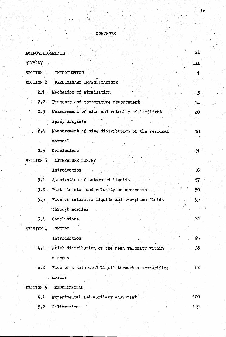
CONTENTS
ACKNO'/ILEDC-EMENTS
SUMMARY
SECTION 1
SECTION 2
2.1
2.2
2.3
INTRODUCTION
PRELIMINARY INVESTIGAliONS
Mechanism of atomization
Pressure and temperature measurement
Measurement of size and velocity of in-flight
spray droplets
2,4 Measurement of size distribution of the residual
aerosol
2 • .5 Conclusions
SECTION 3 LITERATUllE SURVEY
Introduction
Atomization of saturated liquids
Particle size and velocity measurements
Flow of saturated liquids ~d two-phase fluids
through nozzles
3,4 Conclusions
SECTION 4 THEORY
Introduction
- 4,1 Axial distribution of the mean velocity within
a spray
4,2 Flow of a satu•~ted liquid through a two-orifice
nozzle
SECTION .5
_5,1
5.2
EXPERIMENTAL
Experimental and auxilary equipment
Calibration
ii
iii
1
.5
14
20
28
31
36
37
.50
5.5
62
65
68
82
100
119
iv
5.3 Experimental programme
5.4 Experimental procedure
SECTION 6 EXPERIMENTAL RESULTS AND COMPARISON WITH THEORY
6.1 Determination of the values of the constants
c1, c2, c3 and '1
6.2 Measurement of mass flow-rate and comparison
with theoretical expressions for the flow-rate
through a single orifice
6.3 Measurement of the temperature fall,AT1 across
the first orifice of the nozzle assembly and
comparison with theory
6.4 Experimental verification of the expression for
the mass flow-rate through a two-orifice nozzle
assembly
6.5 Measurement of the relative velocity between
liquid and. gas phases at the exit of the nozzle
6.6 Measurement of the exit velocity of .the spray
and comparison with theory
120
124
133
135
145
154
165
169
172
6.7 Measurement of the transverse profile of longitudinal 180
velocity within the spray
6.8 Measurement of the divergence angle of the spray
6.9 Measurement of the longitudinal profile of
longitudinal velocity within the spray and
comparison with theory
6.1 0 Measurement of the variation or' particle velocity
within a spray with particle size, and comparison
with standard theory
187
192
204
6.11 Determination of the size analyses of the resultant 216
surfactant aerosols and their variation with nozzle
dimensions
V
I
I
6,12 Determination of the degree of metastability of
the propellant in the expansion chamber
223
SECTION 7 CONCLUSIONS AND RECOMMENDATIONS FOR FURTHER WORK 225
APPENDIX
1,1 Nozzle dimensions
1,2 Mass flow-rate
1,3 Temperature and pressure measurements of the
propellant during nozzle flow
1.4 Vr.riation of particle velocit:r within a spray
with the distance from the nozzle
1,5 Size distribution of solute aerosol.
2 Interferometric photomicrography of flattened
droplets on a glass slide
3
4
Critical flow of air through some of the orifices
· used to form two-orifice nozzle assemblies
Stereoscan electronmiorography of residual aerosol
droplets
NOMENCLATURE
BIBLIOG-RAPHY
233
234
235
236
242
248
252
255
257
261
vi
vii
LIST OF FIGURES
Cross section of a metered-spray generator
Photography of a metered-spray
High speed cine photographs of the expansion chamber and nozzle
2.4 E-Ii:~h speed cine photographs of the expansion chamber and nozzle
High speed. cine ~}H) ~ct;ru::):.s o" '" tl-~ f'~ .. -~~~. t :flc·,·; ce>ntimetres of spray 2.5
2.6 High speed cine photographs of the development of' a metered-spray
2.7 Spray-front development of a metered-spray
2.8 Variation of spra~front velocity with distance from the nozzle
for metered-sprays
Instantaneous pressure and temperature measurement in the
expansion chamber of' a metered-spray generator
2.10 Pressure and temperature measurement in the expansion chamber
of a metered-spray generator
2.11 Temperature and pressure measurement within the expansion chamber
2.12(a)
2.12(b)
2.13
2.14
2.15
of' a metered-dose aerosol generator
Holography of a metered-spray
Reconstruction of a hologram - experimental arrangement
Hologram of a metered-spray
Reconstruction of the above hologram
Size distribution of resultant "Span 85" aerosol from a
metered-spray (Log. probability plot)
2.16 Size diatribution of resultant "Span 85" aerosol from a
metered-spray (Rosin-Rammler plot)
2.17 Photograph of the discharge of a metered-spray
3.1 Dependence of the size distribution of kerosene aerosol
on various parameters
viii
4.1 Development of a turbulent circular air jet
4.2 Scale draWing of a continuous spray taken f'rom f'lash a.tld long
exposure photographs
4.3 Flow of a two-phase fluid through a short tube
Variation of critical pressure ratio (r ) with the ratio c
by volume of' vapour to liquid (X ) · . 0
·5.1 Diagram of the apparatus
5.2 Nozzle assembly
5.3 General view of the experimental apparatus
5.4 TWo-dimensional movement
5,5 Nozzle assembly
5.6 Photomicrograph~o unit
5.7 Double spark unit and camera
5.8 Variation of depth of field of the camera with aperture
setting
5.9 Temperature of the propellant in the nozzle assembly
5,10 Determination of the "Spread Factor" for a flattened droplet
6.1 Double-flash photomicrograph of aerosol spray
6.2 Flow of saturated propellant through two-orifice nozzle
assembly
6.3 The Clapeyron equation applied to a solution of propellants 12
and 11
6.4 Discharge of propellant through the upstream orifice
6.5 Discharee of propellant through the downstream orifice
6.6 Discharee of propellant through the do1mstream orifice
6.7 Effect of increase in height of the propellant cylinder on·
the flow through a twin-orifice nozzle
-- ----------------------------------
6.8 Effect of increase in the temperature of the propellant on
the flow through a twin-orifice nozzle
6.9 Temperature fall across the upstream orifice
6.10 Mass flow-rate through a two-orifice nozzle
6.11 Comparison between sonic velocity and non-choking exit
velocity
6.12 Transverse profile of longitudinal velocity
6.13 Transverse variation of longitudinal velocity within a spray
6.14 Comparison between the turbulence of an air jet and that of
6.15(al (b 6.16~~
6.17~~~
6.18(a) (b)
6.19
6.20
A 2.1
A 2.2
A .).1
A 4.1
an experimental spray
Longitudinal profile of longitudinal velocity
Axial velocity profile
Prediction of the relative velocity between particle and
gaseous componant of a spray
Size distribution of the resultant surfactant aerosol from
various nozzles
Variation of aerosol size distribution with,nozzle diameter
Metastability of the propellant in the expansion chamber
Interferometric photomicrography of droplets
Photomicrograph of droplets, showing the presence of
interference fringes
Critical flow of air through various single orifices
Stereoscan electror~icrographs
X
.·',
, LIST OF TABLES
3.1 Effect of nozzle type on size distribution of a kerosene aerosol
3.2 The influence of several formulation parameters on particle size
3.3 Effect of the viscosity· of the solute on the size distribution
of the solute aerosol
6.1 Determination of velocity ratio between liquid and vapour phases;
variation of exit velocity with particle size
6.2 Comparison between the measured exit velocity of the spray and
calculated values
6.3 Estimation of the position of the spray origin obtained by
macrophotography of the spray
6.4 Determination of the exit v&locity of the propellant from
several nozzles
6.5 Size analyses of the solute aerosol
1
1 INTRODUCTION
The purpose of the work described in this thesis was to investigate
the operation of liquified-gas aerosol generators as a means of dispersing
a powder and administering it into the deeper recesses of the respiratory
tract; the powder of interest was a metered dose of a micronised drug.
The size distribution of the drug, necessary to achieve optimum administration
is not known precisely, but it is generally agreed ( 8,25;42) that because
of deposition by impaction and sedimentation the probability of particles
ot diameter above 3 to 5 /l m reaching the required area of the lungs is low.
Further there is a diameter of minimum deposition which represents
particles too small for deposition by impaction or sedimentation but too
large for deposition by the alternative means, which is diffusion; this
diameter is about -! /l m. Thus a suitable 'size distribution may well be one
in which the mass of the drug is concentrated in the above particle size
range, 5 pm to -!/lm.
It is possible to produce the drug in powdered form, whose size
distribution corresponds approximately to that given above. However, it
is found that generally the size distribution of the drug is not renroduced . . in either that of the emitted spray or the residual aerosol. The latter
distributions are generally coarser than that of the drug, and therefore
efficiency of deposition is impaired. The reason that the emitted spray
is coarser than the drug is that the spray is in the form of incompletely
evaporated propellant droplets which tend to be larger than, and contain,
the drug particles. The reason that the residual aerosol may be coarser
than the drug is two-fold. Firstly, each emitted droplet may contain
more than one drug particle; this tendency will depend on the size
distribution of the spray droplets, ru1d the concentration of the drug for
a given drug size distribution. The second reason is that a non-volatile ·
surface active agent is included in the formulation. Thus the residual
2
aerosol will consist of one or more drug particles in a surfe.ctant droplet;
there may of course be surfactant droplets with no drug, The reason for
including the surfactant in the formulation is to ensure that the d~lg does
not coagulate prior to use, and to ensure smooth operation of the special
metering valve, The relative concentrations of the drug and surfactant
are typically 0.2% and'1% respectively,
A further point may be made regarding the position of deposition of
the drug in the respiratory tract. This is that the velocity of the spray
in the vicinity of the nozzle is much greater than that of inspired air
in the region of the throat; the former is of the order of 30 m/sec,
the latter of the order of 1.5 m/sec (35-)· This means that the
probability of a particle impacting on the back of the throat is greatly
enhanced. It follows therefore the velocities of the particles as well
as their diameter are of interest in this study, A measure of the relative
importance of the size and velocity of a particle is given by a
dimensionless impaction parameter (~). This is defined as the ratio of
the particle stop distance to. the spray diameter, and the greater its value
the greater is the probability of impaction, It is given by:-
1 =-18
(particle diameterl (particle velocity) (particle density)
(fluid viscosity) (spray diameter)
The relative importance of the various spray parameters, especially
diameter which is raised to the power 2, is seen from this expression,
In principle an arrangement of baffles could be the solution to many
of the problems associated with aerosol spray therapy. This is because a
baffle could remove undesirabiy large particles and also destroy the momentum
of' the spray. However it is .desirable that the aerosol generator should
be inconspicuous and fast in operation; it should remain clean and not
L_ _________________________________________________ -- --
become coated with spray deposit. This means that baffles or a large
adapter designed to permit attenuation of the spray are not acceptable.
It is clear from the above discussion that optimisation of the
design of therapeutic aerosol generators is a multi-facet problem,
Worthwhile areas of investigation could have included the study of the
flow of fine SUspensions through orifices, atomization of liquified
gases and subsequent spray development, 9r the aerodynamics of particle
flow in regions of restricted geometry. It was considered that the most
prof'i table area of study would probably· be that of atomization and
subsequent spray development. This study was thus persued. The first
part was preliminary experimentation in which commercially produced
metered-spray generators and equipment already· available were used.
.3
From this uork it was found that because of the transient nature of the
metered spray, which was of short duration, its behaviour was not readily
amenable to mathematical description, Therefore after the preliminary
studies had been carried out a· continuous-flow rig was built and further
work carried out on this, Finally, information obtained from the continuous
flow rig was related where possible to the metered spray generator.
Throughout this thesis, halogenated hydrocarbon propellants
(or refrigerants),· for example propellant 12, are identified by an
internationally adopted number coding system stan:iardised by the
huerican Society of Refrigerating Engineers in 1957 (Standard Code ASRE 34)
The A.S.R.E. number system for chemically saturated
chlorofluorohydrocarbons is relat~d to their chemical formulae in the
following way:-
Reading from right to left
First number = number o!' fluorine atoms
Second number = number of hydrogen atoms plus ·~ne
Third number = number of carbon atoms minus one
Thus, propellant 11 is C c13
For trichloromonofluoromethane. Propellant 12
is c c12 r2 or dichlorodichloromethane. Propellant 11~ is c2
c12
r4
or
dichlorotetrafluoroethane.
Mention may also be made of the use of mathematical symbols. Owing
to the limitations of the typewriter,· consistency in the mathematical
symbol for multiplication was difficult to maintain. Thus "x" was used
in the absence of the algebraic symbol "x" for distance, otherwise
brackets or a point were used. Similar difficulty was experienced with
the differential operator "d" and the algebraic symbol "d" for particle
diameter. In the presence of the latter, a derivative was placed in
brackets.
2, PRELllliNARY INVESTIGATIONS
2,1 Mechanism of atomization
2,2 Pressure and temperat?re measurement
2,3 Measurement of size and velocity of in-flight spray droplets
2.4 Measurement of size distribution of the residual aerosol
2.5 Conclusions·
An initial survey of the literature indicated that there had been
little investigation into the basic mechan!sms of the atomization of
the saturated liquids, However, much work had been done on the analysis
of what is often the end product, an aerosol of' f'ine solute particles,
In this work, preliminary experimentation was carried out with
the purpose of obtaining a qualitative, and to a certain extent
quantitative, concept·of the mechanism of atomization, Also, the
feasibility of various methods of particle size analysis as applied to
aerosols was assessed. These tests were carried out in a laboratory
maintained at a temperature of about 15°C to 20°c.
2,1 Preliminary investigations into the mechanism of atomization
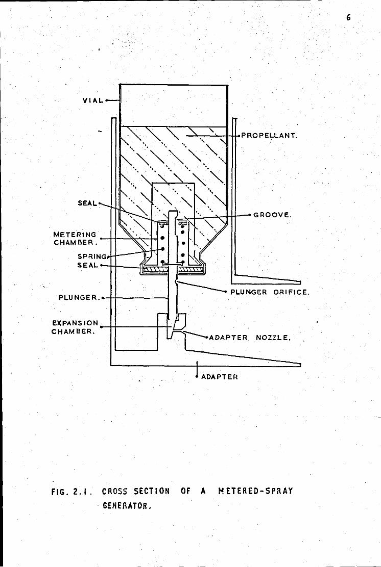
Initial investigations were carried out on sprays generated by a
metering device. This allowed 25mm3 (or 50mm3) of a liquified gas
propellant to pass through a nozzle in a high-density polythene adapter,
a section of which is shown in Figure 2.1. The propellant consisted of,
by weight, 50% propellant 12, 25% propellant 11 and 25% propellant 114,
5
into which was dissolved 1% by weight of the surface-active agent, sorbitan
trioleate ("Span 85 11 ). At 20°C the saturated vapour pressure of' the propellant
was approximately 300 kN/m2 gauge (43 p.s.i.g.), Because the molecular weight
of the sorbitan trioleate (962) is high compared with propellru>ts 12,11 and 114
(121,137 and 171 respectively),tha introduction of the solute in this
· concentration will have negligible effect on the iWP of' the propellant.
In Figure 2.1, the metering chamber is shown filled with propellant
which had entered through the groove in the plunger. The spray was
6
VI AL.
SEAL.
PL.UNGER.~H---------~ r------..... PL.UNGER ORIFICE.
EX PANS I 0 N -1+-------+-+ CHAMBER.
NOZZL.E.
ADAPTER
FIG. 2.1. CROSS SECTION OF A METERED-SPRAY
· GENERATOR.
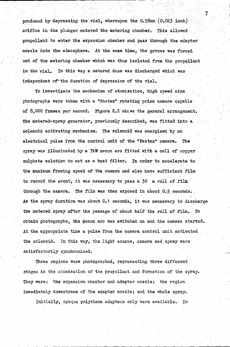
produced by depressing the vial, whereupon the 0,58mm (0,023 inch)
orifice in the plunger entered the metering chamber, This allowed
propellant to enter the expansion chamber and pass through the adapter
nozzle into the atmosphere, At the same time, .the groove was forced
out of the metering chamber which was thus isolated from the propellant
in the vial, In this way a metered dose was discharged which was
independent o~the duration of depression of the vial,
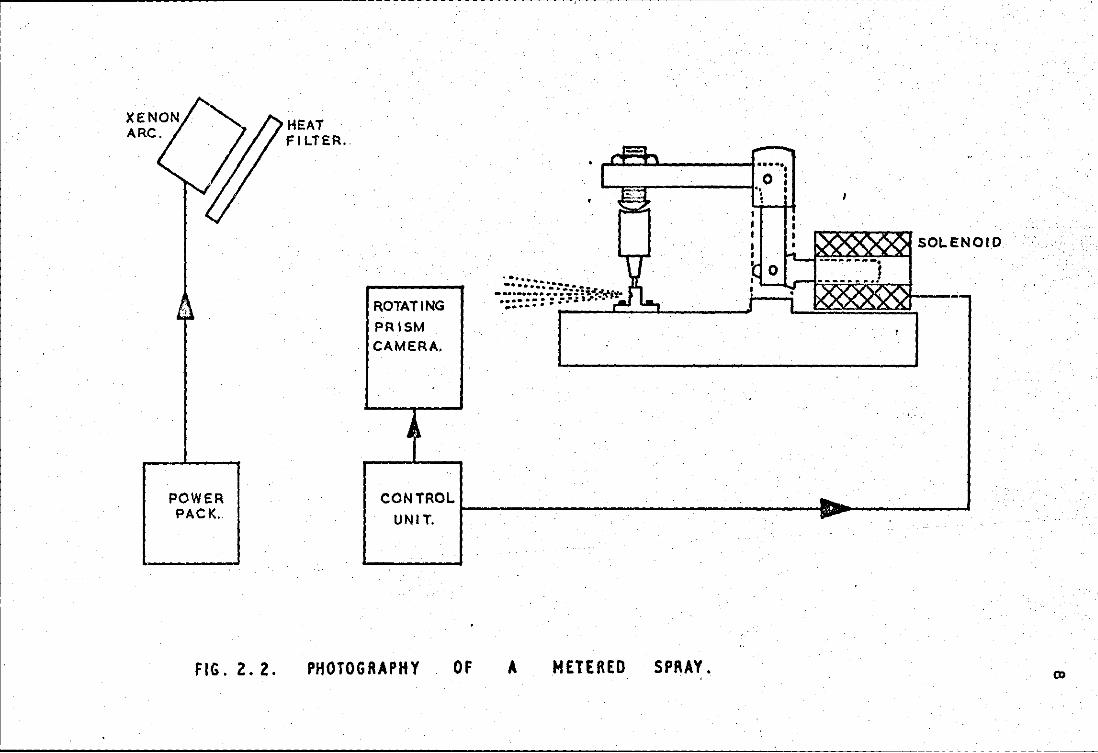
To investigate the mechanism of atomization, high speed cine
photographs were taken with a "Fastax• rotating prism camera capable
of 8,000 frames per second. Figure 2.2.shcns the general arrangement,
The metered-spray generator, previously described, was fitted into a
solenoid activating mechanism. The solenoid was energised by an
electrical pulse from the control unit of the "Faatax" camera. The
spray was illuminated by a 7kW xenon arc fitted with a cell of copper
sulphate solution to act as a heat filter. In order to accelerate to
the maximum framing speed of th~ camera and also have sufficient film
to record the event, it was necessary to pass a 30 m roll of film
through the camera, The film was then exposed in about 0,5 seconds,
7
As the spray duration was about 0,1 seconds, it was necessary to discharge
the metered spray after the passage of about half the roll of film, To
obtain photographs, the xenon arc was switched on and the camera started,
At the appropriate time a pulse from the camera control unit activated
the solenoid. In this way, the light source, camera and spray were
satisfactorily synchronised,
Three regions were photographed, representing three different
stages in the atomization of the propellant and formation of the spray.
They were: the expansion chamber and adapter nozzle; the region
immediately downstream of the adapter nozzle; ~~d the whole spray,
Initially, opaque polythene adapters only were available, In
POWER PACK.
FIG. 2.2.
HEAT FILTER.
ROTATING
PRISM CAMERA.
= • I
~ • .
...., .... -.*:.·.-.-..· .. -········· .......... ........... ·.-:.-... 1.,
-- --· "'-~i'!-........... ·;.
• ••••• 0 • I .. I ; I
I I
' I
' I l'-' ' • I .. 1.. XXX
~ 0 - --------. ---- ... J •
! "! rx>S&xw I I
'
CONTROL
~-----------------------------UNIT.
PHOTOGRAPHY OF A METERED SPRAY.
SOL ENOIO
order to observe the propellant 'behaviour in the expansion chamber
and nozzle, a section of the adapter was milled away until the expansion
chamber and nozzle were revealed. The milled section 1vas then replaced
by a strip of perspex, 3.2 mm. (i- inch) thick, which was bolted to
the adapter. Eventually transparent tenite butyrate adapters were
obtained, and in this case no milling was required.
9
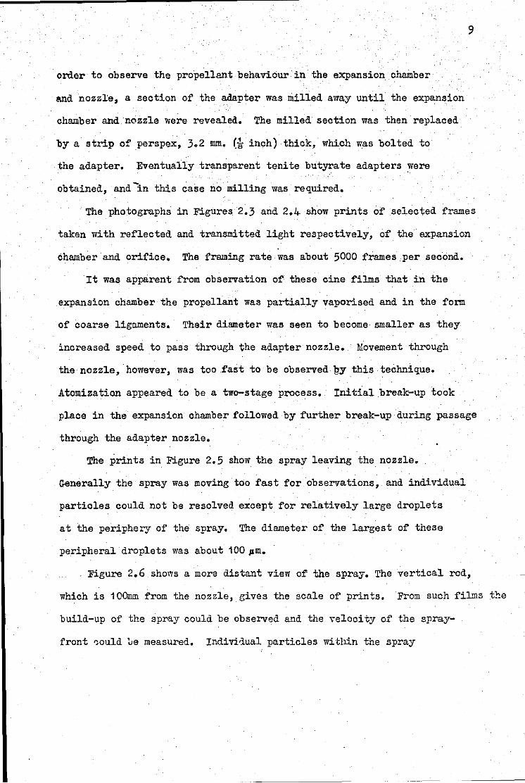
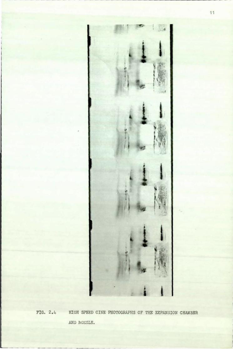
The photographs in Figures 2.3 and 2.4 show prints of .selected frames
taken with reflected and transmitted light respectively, of the expansion
chamber and orifice, The framing rate was about 5000 frames per second.
It was apparent from observation of these cine films that in the
expansion chamber the propellant was partially vaporised and in the form
of coarse ligaments, Their diameter was seen to become smaller as they
increased speed to pass through the adapter nozzle. Movement through
the nozzle, however, was too.fast to be observed gy.this technique.
Atomization appeared to be a two-stage process.· Initial break-up took
place in the expansion chamber followed by further break-up during passage
through the adapter nozzle,
The prints in Figure 2.5 show the spray leaving the nozzle,
Generally the spray was moving too fast for observations, and individual
particles could not be resolved except for relatively large droplets
at the periphery of the spray. The diameter of the largest of these
peripheral droplets was about 100pm.
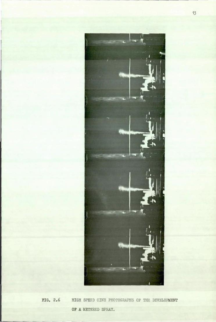
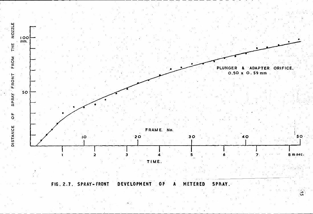
Figure 2,6 shows a more distant view of the spray, The vertical rod,
which is 1 OOmm from the nozzle, gives the scale of prints. From such films .the
build-up of the spray could be observed and the >elocity of the spray-
front '}Ould lie measured, Indivi•lual particles within the spray
FIG. 2 .3 HIGH SPEED CINE PHOTOGRAPHS OF THE EXPANSION CHAMBER
AND NOZZLE.
10
11
l
. •
•
FlG. 2.4 HIGH SPEED CINE PHOTOGRAPHS OF 'l'HE EXPANSION CHAMBER
AND .f.IOZZLE.
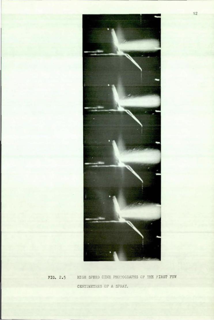
FIG. 2. 5 HIGH SPEED C TNE f'HO OGRAT HS OF THE r I RST FF:N
CEN'l'HIETRES OF A SPRAY.
12
------------------------------------------------------------------
F.I(}. 2 . 6 HIGH SPEED CINE PHOTOGRAPHS OF THE DEVELOPYENT
OF A ID;TERED SPRAY.
13
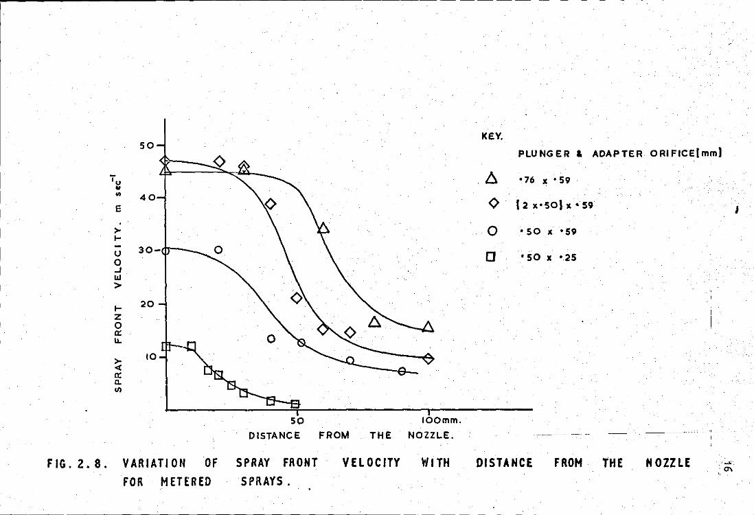
could not be resolved, however. A. graph of the variation of spray
front position \fith time is shown in Figure 2.7, while Figure 2.8
shows the variation of spray-front velocity with distance from the
nozzle.
14
It is seen that, over the first few centimetres, the velocity of
the spray-front remains essentially c.onstant. Beyond this distance
air is entrained into the spray by turbulent mixing and the spray
front velocity decays rapidly. Unfortunately.it was not possible tc-
measure velocities within the spray behind its front boundary.
Although no precise correlation between spray-front velocity and
nozzle .diameter was obtained, it is significant that the adapter with
a 0.25 mm. (0.010 inch) nozzle generated a very low-velocity spray.
This is to be expected on theoretical grounds as explained in
Section 4.
From photographs of the complete spray, it was possible to measure
the total volume of the spray. It was found that the latter was many
times greater than the volume of vapour available from the metered
volume of propellant. For example, the spray depicted in Figure 2.6
developed into a cone whose volume was approximately 70 x 1 c} m.'ll3• Now
. -~ 3 the volume of vapour.from 25 mm3 of propellant is only 6 x 1~ mm. Therefore
the resultant spray consisted of a surfactant aerosol in a gas phase
comprising approximately 907-G entrained 'air and 10% propellant vapour •.
2.2 Pressure and temperature measurements within the exoansion
cham'cer
Atomization and velocity of discharge through a noz3le are
intimately related to the pressure across the nozzle and to the
liquid-to-gas ratio passing through it, the latter depending upon the
propellant temperature. It was therefore desirable to measure the
temperature and pressure within the expansion chamber.
w ...1 N
'N 0 z 100
w .:r:
1-
:::l 0 a: LL
1-z 0 c: LL
~ 0: a. Ul
LL 0
w u z ~ Ill
Cl
mm.
50
• •
10
2
FIG.?.. 7. SPRAY~ FRONT
20
3
FRAME. No.
4
TIME.
DEVELOPMENT OF
30
•
PLUNGER & ADAPTER ORIFICE.' 0.50" 0. 59 mm
40
•
5 6 7 8 m sec.
A METERED SPI\AY. ' ' ...
\11
KEY. 50
0 RI FICE( mm) PLUNGER & ADAPTER
Tu ~ •76 X •59 .. .. 40 E 0 l2x•SO)x•59 I
>- 0 ... •so x •59
- 30-u 0 0 '50 X •25 .J w >
... 20 z 0 a: u.
>- 10 < a: a. U)
50 lOO mm.
DISTANCE FROM THE NOZZLE.
FIG. 2. 8. VARIATION OF SPRAY FRONT V EL 0 C JTY W I TH DISTANCE FROM THE NOZZLE '-' :0\
FOR METERED SPRAYS.
17
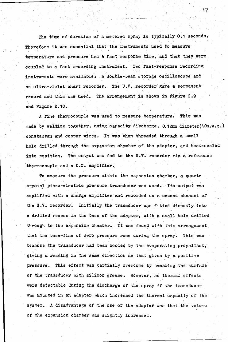
The time of duration of a metered spray is. typically 0,1 seconds,
Therefore it was essential that the instruments used to measure
temperature and pressure had a fast response time, and that they were
coupled to a fast recording instrument. Two fast-response recording
instruments were available; a double-beam storage oscilloscope and
an ultra-violet chart recorder. The U,V. recorder gave a permanent
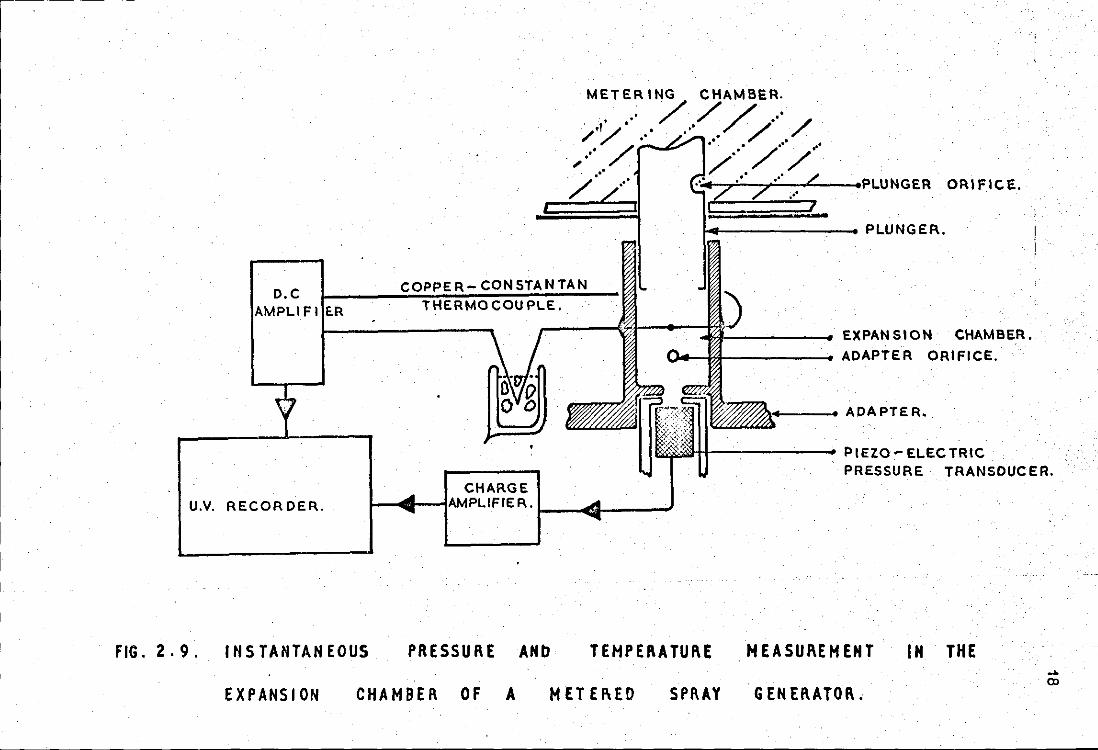
record and this was used, The arrangement is· shown in Figure 2.9
and Figure 2.10.
A fine thermocouple was used to measure temperature. This was
made by welding together, using capacity discharge, 0,12mm diameter(40s,w.g.)
constantan and copper wires, It was then threaded through a small
hole drilled through the expansion chamber of the adapter, and heat-sealed
into position. The output was fed to the U.V. recorder via a reference
thermocouple and a D.C. amplifier,
To measure the pressure within the expansion chamber, a quartz
crystal piezo-electric pressure transducer was used, Its outp.ut was
amplified with a charge amplifier and recorded on a second channel of
the U.V. recorder~ Initially the transducer was fitted directly into
a drilled recess in the base of the adapter, with a small hole drilled
through to the expansion chamber. It was found with this arrangement.
that the base-line of zero pressure rose during the spray. This was
because the transducer had been cooled by the evaporating propellant,
giving a reading in the same direction as that given by a positive
pressure. This effect was partially overcome by smearing the surface
of the transducer with silicon grease, However, no thermal effects
were detectable during the discharge of the spray if the transducer
was mounted in an adapter which increased the ·thermal capacity of the
system. A disadvantage of the use of the adapter was that the voluz,e
of the expansion chamber was slightly increased.
D.C IAlvtPLI F I
U.V. RECORDER.
FIG. 2. 9. ltiS TANTAN EOUS
COP T
CHARGE t-•-1AMPLIFIER.I--Ciil-----'
1------... EXPANSION CHAMBER.
-----ADAPTER ORIFICE.
+1-----'----- PIEZO-ELECTRIC PRESSURE TRANSDUCER.
PRESSURE ANb TEMPERATURE MEASUREHEHT IH THE .... CX>
EXPANSION CHAMBER OF A HETEI\ED SPRAY GENERA TO I\,
19
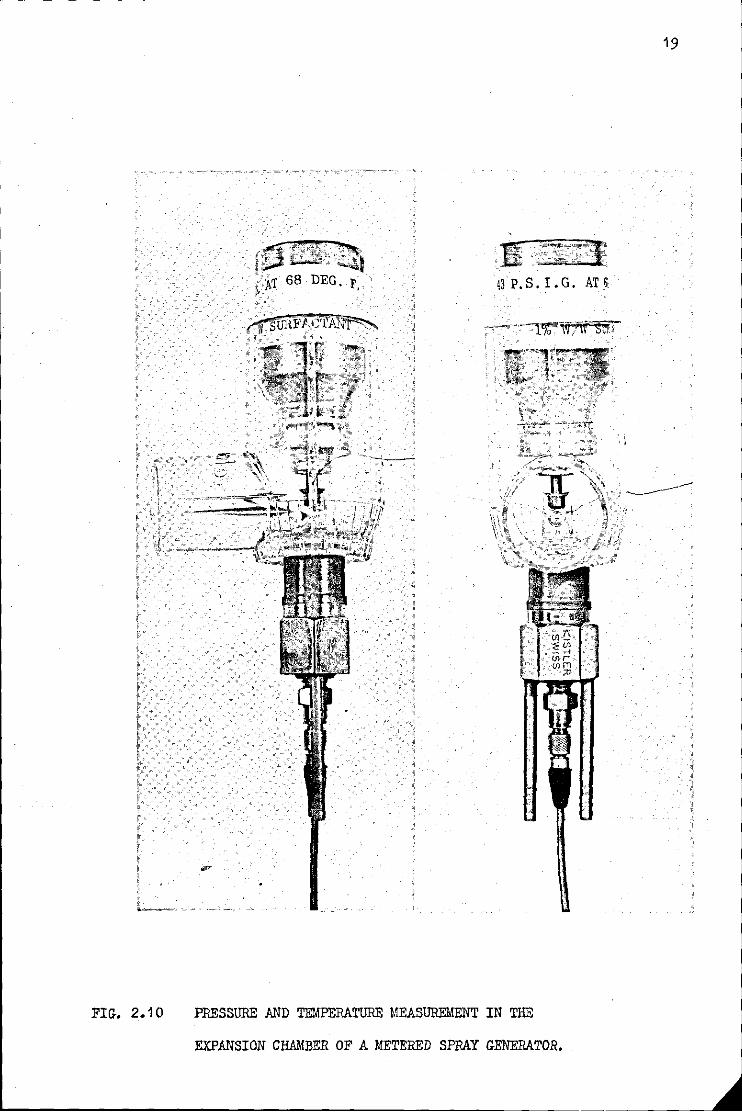
!3P.S. I. G. AT &
FIG. 2.10 PRESSURE AND TEMPERATURE MEASUREMENT IN THE
EXPANSION CHAMBER OF A METERED SPRAY GENERATOR.
20
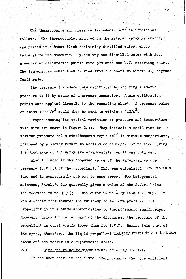
The thermocouple and pressure transducer were calibrated as
follows. The thermocouple, mounted on the metered spray generator,
was placed in a Dewar flask containing distilled water, whose
temperature was measured. By cooling the distilled water with ice,
a number of calibration points were put onto the U.V. recording chart.
The temperature could then be read from the chart to within 0.3 degrees
Centigrade;
The pressure transducer was calibrated by applying a static
pressure to it by means of a mercury manometer. Again-calibration
points were applied directly to
. I 2 of about 100kN m could then be
the recording char.t. A pressure pulse
read to within± 1kN/m2 •
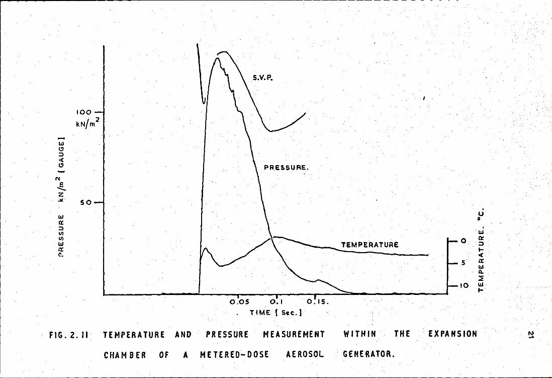
Graphs showing the typical variation of pressure and temperature
with time are shown in Figure 2.11. They indicate a rapid rise to
maximum pressure and a simultaneous rapid fall to minimum temperature,
followed by a slower return to ambient conditions. At no time during
the discharge of the spray are steady-state conditions obtained.
Also included is the computed value of the saturated vapour
pressure (S.V.P.) of the propellant.· This was calculated from Raoult's
Law, and is consequently subject to some error. For halogenated
methanes, Raoult's Law gener'ally gives a value of the S.V.P. below
the measured value.( 7 ); the error is usually less than 10%. It
would appear that towards the build-up to maximum pressure, the
propellant is in a state approximating to thermodynamic equilibrium.
However, during the latter part of the discharge, the pressure of the
propellant is considerably low_er than its S.V.P. During this part of
the spray, therefore, the liquid propellant probably eY~sts in a metastable
state and the vapour in a superheated state.
2.3 Size and velocity measurements of snray droplets
It has been shovm in the introductory remarks that for efficient
-w Cl :;) <( Cl -
w a: :;)
Ul Ul w a: c.
so
S.V.P.
PRESSURE.
0.05 0.1
TIME [Sec.)
FIG. 2.11 TEMPERATURE AND PRESSURE MEASUREMENT
CHAMBER OF A METERED-DOSE AEROSOL
WITHIN THE
GENERATOR.
0
5
• 0 0 . ·w ~ :;) ... < a: w
.Q.
~ 10 w ...
EXPANSION
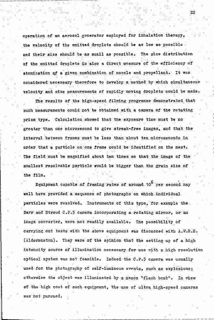
operation of an aerosol generator employed for inhalation therapy,
the velocity of the emitted droplets should be as low as possible
22
and their size should be as sm~ll as possible. The size distribution
of the emitted droplets is also a direct measure of the efficiency of
atomization ~f a given combination of nozzle and propellant. It was
considered necessary therefore to develop a method by which simultaneous
velocity and size measurements of rapidly moving droplets could. be made.
The results of the high-speed filming programme demonstrated_ that
such measurements could not be obtained with a camera of the rotating
prism type. Calculation showed that the exposure time must be no
greater than one microsecond to give streak-free images, and that the
interval between frames must be less than about ten microseconds in
order that a particle on one frame could be identified on the next.
The field must be magnified about ten times so that the image of the
smallest resolvable particle would be bigger than the grain size of
the film. . . . . . 6
Equipment capable of framing rates of around 10 per second may
well have provided a sequence of photographs on which individual
particles \?ere resolved. Instruments of this type,· for example the.
Barr and Stroud C.P.5 camera incorporating a rotating mirror, or an
image converter, were not readily available. The possibility of
carrying out tests with the above equipment was discussed with A.IV.R.E.
(Aldermaston). They were of the opinion that the setting up of a high
intensity source of illumination necessary for use with a high resolution
optical system was no~ feasible. Indeed the C.P.5 camera was usually
used for the photography of self-luminous &vents, such as explosions;
otherwise the object was illuminated by a .Xenon "flash bomb". In view
of the high cost of such equipment, the use of ultra high~speed cameras
was not pursued.
23
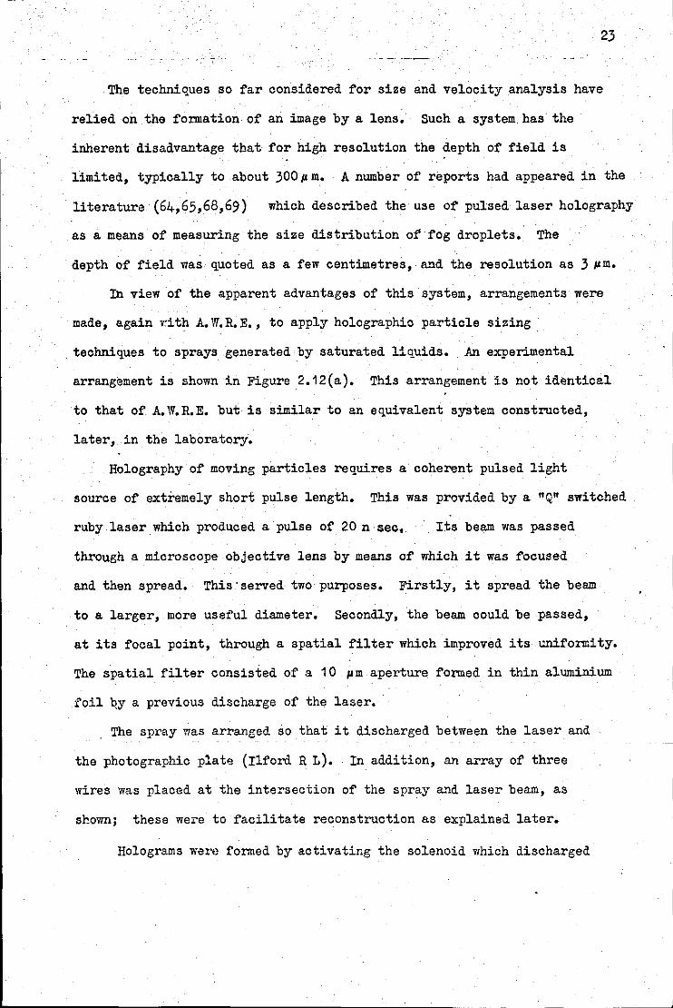
The techniques so far considered for size and velocity analysis have
relied on the formation. of an image by a lens. Such a system. has the
inherent disadvantage that for high resolution the depth of field is
limited, typically to about 300 pm. A number of reports had appeared in the
literature (64,65,68,69) which described the use of pulsed laser holography
as a means of measuring the size distribution of fog droplets. The
depth of field was quoted as a few centimetres, and the resolution as 3 pm.
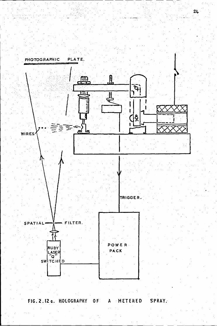
In view of the apparent advantages of this system, arrangements were
made, again v:ith A. W.R.E., to apply holographic particle sizing .
techniques to sprays generated by saturated liquids. An experimental
arrangement is shown in Figure 2.12(a). This arrangement is not identical
to that of A.W.R.E. but is similar to an equivalent system constructed,
later, in the laboratory.
Holography of moving particles requires a coherent pulsed light
source of extremely short pulse length. This was provided by a "Q" switched
ruby laser.which produced a pulse of 20 n·sec, Its beam was passed
through a microscope objective lens by means of which it was focused
and then spread. This·served two purposes. Firstly, it spread the beam
to a larger, more useful diameter. Secondly, the beam could be passed,
at its focal point, through a spatial filter which improved its uniformity.
The spatial filter consisted of a 10 pm aperture formed in thin aluminium
foil ~y a previous discharge of the laser •
. The spray was arranged so that it discharged between the laser and
the photographic plat~ (Ilford R L). In addition, an array of three
wires was placed at the intersection of the spray a.'ld laser beam, as
shown; these were to facilitate reconstruction as explained later.
Holograms were formed by activating the solenoid vthich discharged
I
I
PHOTOGRAPHIC PLATE,
••• WIRES
SPATIAL-- FILTER.
. RUBY LASE •• Q ,,
FIG. 2 .12 a. HOLOGRAPHY 0 F
TRIGGER.
POWER
PACK
A METERED SPRAY.
-1:::1J== : : ~ I He Ne LASER.
-SPATIAL HOLOGRAM FILTER CAMERA
I with I ens remove cl J
~---·
FIG. 2.12 b. RECONSTRUCTION OF A HOLOGRAM.
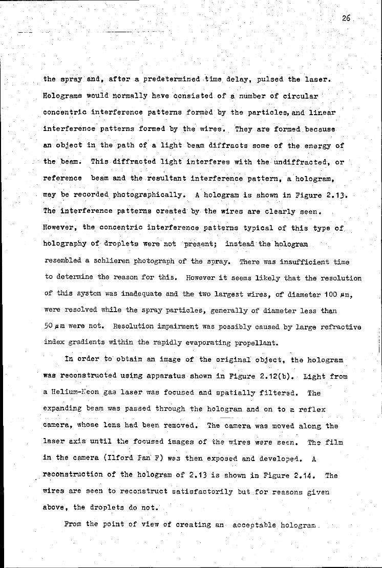
the spray and, after a predetermined time. delay, pulsed the laser.
Holograms would normally have consisted of a number of circular
concentric interference patterns formed by the particles,and lir.ear
interference patterns formed by the wires. They are formed because
26.
an object in the path of a light beam diffracts some of the energy of
the beam. This diffracted light interferes with the undiffracted, or
reference beam and the resultant interference pattern, a hologram,
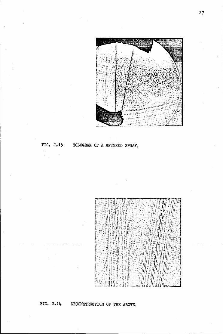
may be recorded photographically. A hologram is shown in Figure 2.1).
The interference patterns created by the wires are clearly seen.
However, the concentric interference patterns typical of this type of
holography of droplets were not present; instead the hologram
resembled a schlieren photograph of the spray. There was insufficient time
to determine the reason for this. However it seems likely that the resolution
of this system was inadequate and the two largest wires, of diameter 100 Jlm,
were resolved while the spray particles, generally of diameter less than
50 )lffi were not. Resolution impairment was possibly caused by large refractive
index gradients within the rapidly evaporating propellant.
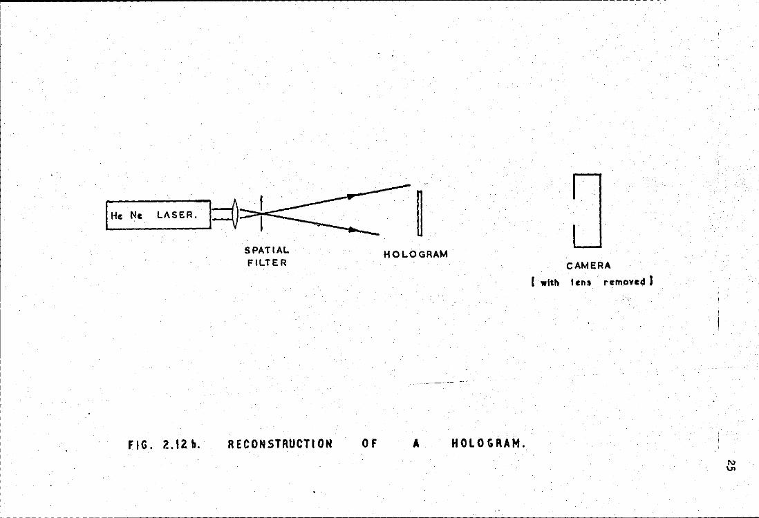
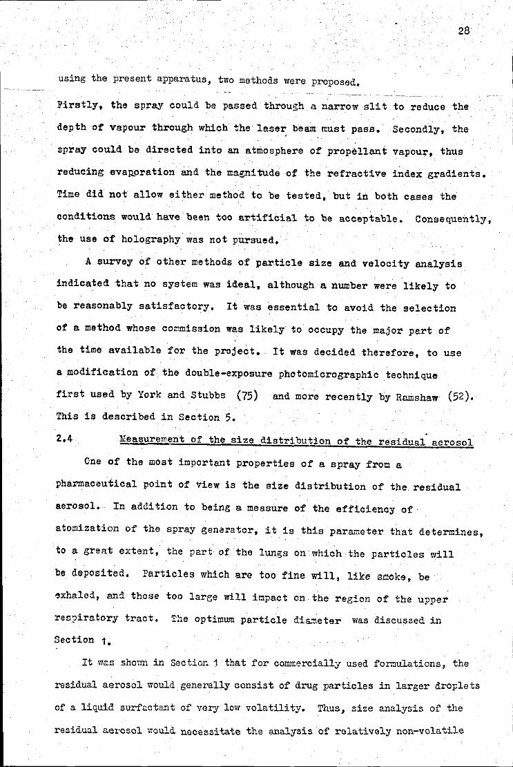
In order to obtain an image of the original object, the hologram
was reconstructed using apparatus shown in Figure 2.12(b), Light from
a Helium-I:eon gas laser was focused and spatially filtered. The
expanding beam was passed through the hologram and on to a reflex
camera, whose lens had been removed, The camera was moved along the
laser axis until t~e focused images of the wires were seen. The film
in the camera (Ilford Fan· F) wa3 then exposed and develope1. A
reconstruction of the hologram of 2.13 is shown in Figure 2.14. The
wires are seen to reconstruct satisfactorily but for reasons given
above, the droplets do not.
From the point of view of creating an acceptable holograffi_
27
FIG. 2.13 HOLOGRAM OF A METERED SPRAY.
FIG. 2.14 RECONSTRUCTION OF THE ABOVE.
28
using the present apparatus, two methods were proposed,
Firstly, the spray could be passed through a narrow slit to reduce the
depth of vapour through which the laser beam must pass. Secondly, the ' .
spray could be directed into an atmosphere of propellant vapour, thus
reducing evaRoration. and the magnitude of the refractive index gradients.
Time did not allow either method to be tested, but in both cases the
conditions would have been too artificial to be acceptable. Consequently,
the use of holography was not pursued,
A survey of other methods of particle size and velocity analysis
indicated that no system was ideal, although a number were likely to
be reasonably satisfactory. It was essential to avoid the selection
of a method whose co~mission was likely to occupy the major part of
the time available for the project, . It was decided therefore, to use
a modification of the double-exposure photomicrographic technique
first used by York and Stubbs (75) and more recently by Ramshaw (52).
This is described in Section 5.
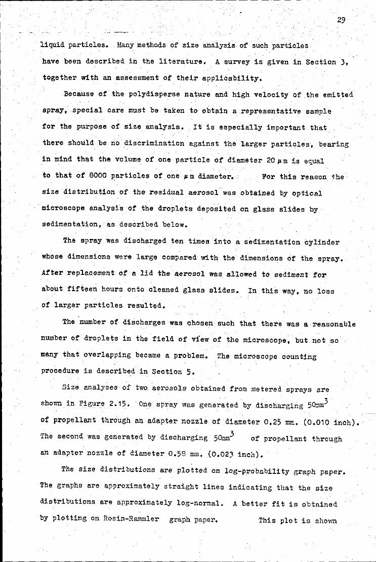
2.4 Measurell'ent of the size distribution of the residual aerosol
One of the most important properties of a spray from a
pharmaceutical point of view is the size distribution of the. residual
aerosol. In addition to being a measure of the efficiency of
atomization of the spray generator, it is this parameter that determines,
to a great extent, the part of the lungs on which the particles will
be deposited, Particles which are too fine will, like sooke, be
exhaled, and those too large will impaet on the reg!on of the upper
recpiratory tract. ~he optimum particle dis.:neter was discussed in
Section 1.
It was shmm in Section 1 that for com!nercially used fonnulations, the
residual aerosol would_ generally consist of drug particles in larger droplets
of a liquid surfactant of very low volatility. Thus, size analysis of the
resid.ual aerosol would necessitate the analysis of relatively non-volatile
29
liquid particles. Many methods of' size analysis of' such particles
have been described in the literature. A survey is given in Section 3,
together with an assessment Of' their applicability,
Because of the polydisperse nature and high velocity of the emitted
spray, special care must be taken to obtain a representative sample
for the purpose of size analysis. It is especially important that
there should be no discrimination against the larger particles, bearing
in mind that the volume of one particle of diameter 20 pm is equal
to that of 8000 P.articles of one pm diameter. For this reason the
size distribution of the residual aerosol was obtained by optical
·microscope analysis of the droplets deposited on glass slides by
sedimentation, as described below.
The spray was discharged ten times into a sedimentation cylinder
whose dimensions were large compared with the dimensions of the spray.
After replacement of a lid the aerosol was allowed to sediment for
about fifteen hours onto cleaned glass slides. In this way, no loss
of larger particles resulted,
The number of discharges was chosen such that there was a reasonable
number of droplets in the field of v!ew of the microscope, but not so
many that overlapping became a problem, The microscope counting
procedure is described in Section 5.
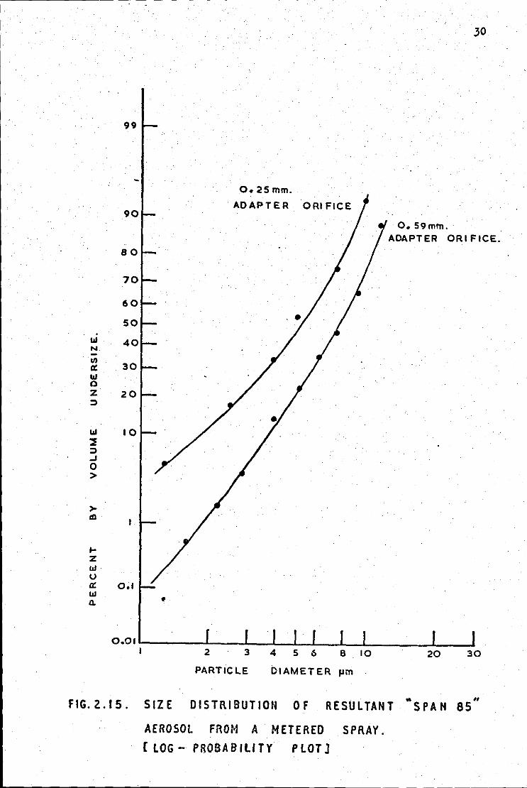
Size analyses of two aerosols obtained from metered sprays are
shown in Figure 2.15. One spray was generated by discharging 50:mn3
of propellant through an adapter nozzle of diameter 0,25 ~. (0.010 inch).
The second was generated by discharging 50mm3 of propellant through
an adapter nozzle of diameter 0.58 m;n, (0,02.3 inch).
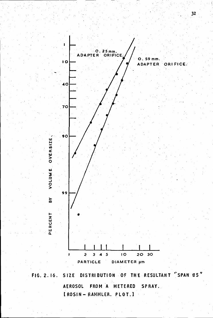
The size distributions are plotted on log-probability graph paper.
The graphs are approximately straight lines indicating that the size
distributions are approximately log-normal. A better fit is obtained
by plotting on Rosin-Rammler graph paper, This plot is shovm
--------------~--------------------------------------------- ~
30
99
o. 2Smm.
ADAPTER ORJ FICE
o. 59 mm. ADAPTER ORIFICE.
"' N -Ill 30 a:
"' 0 z 20 ::)
"' 10 ::e ::) ..J 0 >
>-Ill
,... z Id· u a: o;r
"' ll. •
PARTICLE DIAMETER Jlm
FIG.2.15. SIZE DISTRIBUTION OF RESULTANT .. " SPAN 85
AEROSOL FROf.l A METERED SPRAY.
[LOG- PROBABiliTY PLOTJ
L-~------------~--------~-------------------·-- -
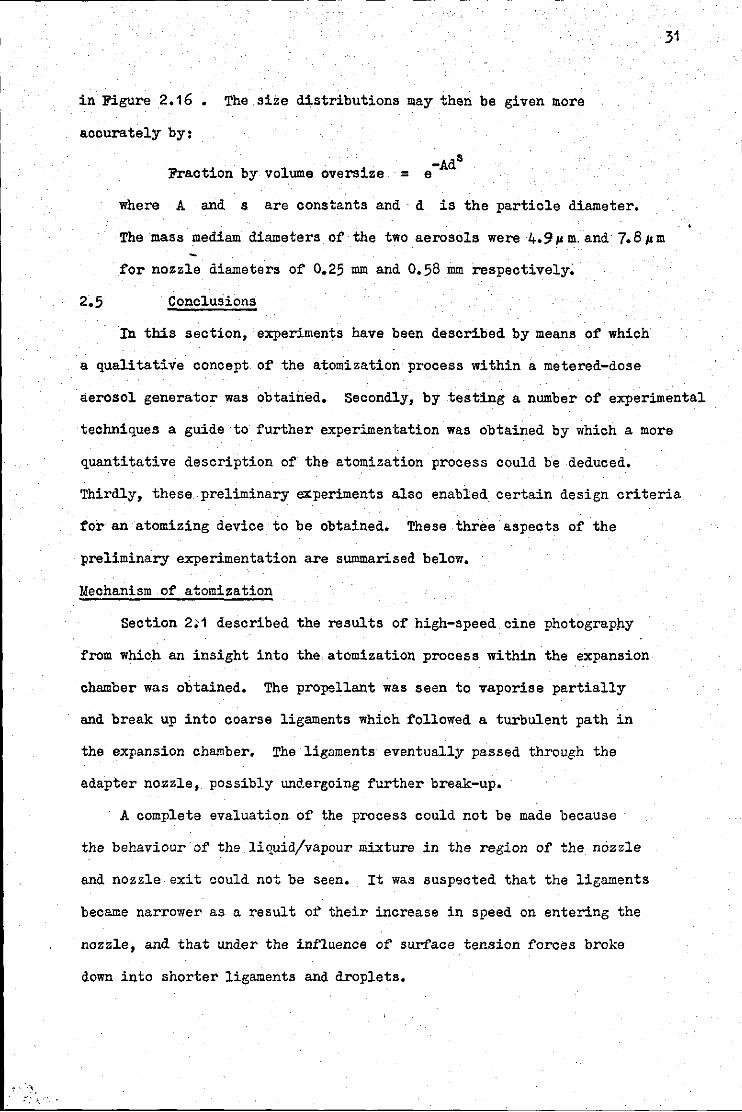
31
in Figure 2,16 • The size distributions may then be given more
accurately by:
Fraction by volume oversize
where A and s. are constants and · d is the particle diameter,
The mass mediam diameters of the two aerosols were 4.9pm.and 7,8pm
for nozzle diameters of 0.25 mm and 0,58 mm respectively~
2.5 Conclusions
In this section, experiments have been described by means of which
a qualitative concept of the atomization process within a metered-dose
aerosol generator was obtained, Secondly, by testing a number of experimental
techniques a guide to further experimentation was obtained by which a more
quantitative description of the atomization process could be deduced.
Thirdly, these preliminary experiments also enabled certain design criteria
for an atomizing device to be obtained. These three aspects of the
preliminary experimentation are summarised below,
Mechanism of atomization
Section 2<1 described the results of high-speed cine photograp~y
from which an insight into the atomization process within the expansion
chamber was obtained. The propellant was seen to vaporise partially
and break up into coarse ligamenta which followed a turbulent path in
the expansion chamber. The ligamenta eventually passed through the
adapter nozzle, possibly undergoing further break-up.
· A complete evaluation of the process could not be made because
the behaviour of the liquid/vapour mixture in the region of the nozzle
and nozzle exit could not be seen. It was suspected that the ligaments
became narrower as a result or their increase in speed on entering the
nozzle, and that under the influence of surface tension forces broke
down into shorter ligaments and droplets.
0. 25mm. AD-APTER ORIFICE.
0. 59 mm. ADAPTER ORIFICE;
10 20 30 2 3 4 5
PARTICLE DIAMETER 11m
32
FIG. 2. 16. SIZE DISTRIBUTION OF THE RESULTANT ··sPAN 85 ''
AEROSOL FROM A METERED SPRAY.
[ROSIN-RAMMLER. PLOT.)
33
Support was given to this view by photomicrographs taken of the
expansion chamber and adapter nozzle by the unit described in Section 5.
One such photograph is reproduced in.Figure 2.17. Although
interpretation is not completely straightforward, the two-phase
mixture in the nozzle is seen to .be highly dispersed, with the liquid
phase in the form of ligaments whose dimensions are considerably
smaller than those of the liga~ents entering the nozzle.
Further experimentation
The above constitutes a limited qualitative description of the
atomization process. It was the purpose of the project, however to obtain
also a quantitative description of this process. This necessitated
in-flight droplet measurements, together with measurements of
temperature and pressure within the expansion chamber of the spray
generator. These could then be' related to the two fundamental
parameters: the dimensions of the nozzle and the thermodynamic
properties of the propellant. These preliminary experiments gave a
guide as to how these measurements might be made.
It is shown in.Section 2.3 that measurements of spray droplets
in flight would require the construction of a double-flash
photomicrographic system. Suitable apparatus was built and used in
subsequent experimentation.
Also, measurements,. described in Section 2.2, of the instantaneous
temperature and pressure of the propellant in the expansion chamber
indicated that satisfactory steady-state conditions were never reached
during the disch~rge of the spray. Under these rapidly varying
conditions it is unlikely that a relationship between properties of
the spray and the spray generator would ha7e been obtained. For these
reasons a continuous-flow model, described in Section 5, was built and
further experimentation carried out under steady-state conditions.
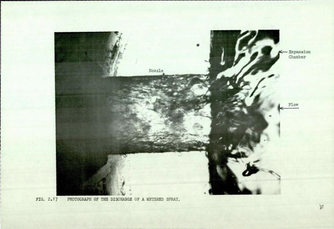
FIG. 2. 17 PHOTOGRAPH OF THE DISCHARGE OF A METZRED SPRAY.
Expansion Chamber
~< Flow
----------------------~------------------------------------------------- -
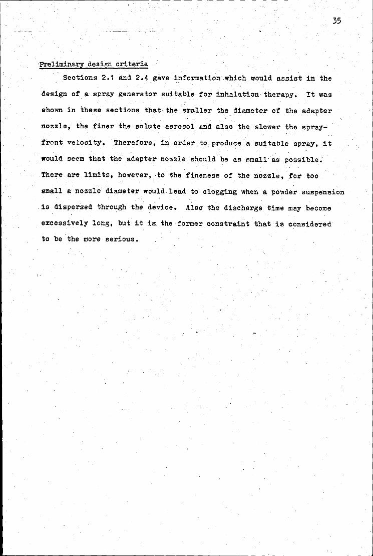
Preliminary design criteria.
Sections 2.1 and 2.4 gave information which would assist in the
design of a spray generator suitable for inhalation therapy. It was
shown in these sections that the smaller the diameter of the adapter
nozzle, the finer the solute aerosol and also the slower the spray
front velocity. Therefore, in order to produce a suitable spray, it
would seem that the adapter nozzle should be as small as. possible.
There are limits, however, -to the fineness _of the nozzle, for too
35
small a nozzle diameter would lead to clogging when a powder suspension
.is dispersed through the device. Also the discharge time may become
excessively long, but it is. the former constraint that is considered
to be the more serious •
.__ ___________________________________________________ -
3 LITERATURF. SURVEY
Introduction
3.1 Atomization of saturated liquids
3.2 Particle size and velocity measurements
3.3 Flow of saturated liquids and two-phase fluids through
nozzles
3.4 Conclusions
Tha areas of general interest in the study of inhalation sprays
or aerosols were outlined in the Introduction, Section 1, while a
preliminary study of the mechanism of atomization of such sprays was
described in Section 2 • It is .the purpose of this section to review
reported work which has a bearing on tha various aspects of this study.
36
37
3.1 Atomization of saturated liquids.
The use of liquified gases as a spray generating agent grew rapidly
during the Second World War. They were used mainly in the application of
insecticides. The propellant then available was the halogenated hydrocarbon,
dichluorodifluoromethane (propellant 12), whose saturated vapour pressure
0 2 (S.V.P.) at room temperature (20 C) is 568 kN/m (abs). It was atomized
through capillary tubing. Owing to the relatively high S.V.P. of this
propellant it had to be housed in strong metal containers, which were
consequently inconvenient and expensive.
Because of the disadvantages of using a high pressure propellant,
new propellants of lower pressure were sought and also efficient means
of atomizing them. The lower pressures were achieved by the development
of halogenated hydrocarbons, of low S,V.P., which were miscible with
propellant 12. Such a compound is trichloromonofluoromethane, or propellant
11, Thus a continuous range of pressures was a:vailable, from 90 kN/m2(abs)
the S.V.P. of propellant 11 at 20°C to 568 kN/m2(abs), as previously
mentioned. Means of atomizing these low pressure propellants were sought.
It was found that the capillary device was still satisfactory, but other
means were investigated, In particular the two-orifice nozzle assembly
for this use was developed in 1950 ( 76 ).
The operation, fop continuous flow, of a two-orifice assembly was
fcund to be as follows, The pressure drop across the first orifice caused
vaporisation of the propellant within the expansion chamber. A two-phase
mixture of propellant liquid and vapour then flowed through the second
orifice. Because liquid only, tended to flow through the first(upstream)
orifice only about one eigth of the overall pressure differential was
dropped across thiz orifice. Thus a substantial fraction of the pressure
differential was available at the second orifice. Atomization was considered
to be a two-stage process. Initial break-up took place in the expansion
chamber as a result of the initial evaporation of the propellant.
Further break-up took place as the resulting two-phase propellant passed
through the second orifice.
.38
Atomization through capillary tubes was similar. In this case however
the process took place continuously over a few centimetres of the tubing.
Most of the work done on atomization through two-orifice nozzle
assemblies has resulted in empirical relationships. These have usually
been a correlation between the size distribution of the resultant aerosol
of the active ingredient and various parameters such as nozzle dimensions,
propellant pressure, proportion of propellant to active ingredient etc.
Experimentation of a more fundamental nature has been performed on atomization
through single-orifice devices however. Work on atomi.zation through two
orifice nozzles and to a certain extent capillary tubing will be considered
first.
Fulton et al ( 19 ) described the atomization of a formulation
consisting of 43% propellant 11, 43% propellant 12 and 14% insecticide
through capillary tubes. A size analysis was performed on the residual
insecticide aerosol and the mass mediam diameter (M.M. D.) was relat.ed to
capillary length and diameter. It was found that for a given capillary
diameter, an optimum length produced a minimum M. M. D. However, over a
range of capillary diameters from 0.34mm to 0. 74mm this minimum M. M. D. was
approximately constant and equal to 16pm.
Two-orifice nozzles were also tested. It was foup.d that the most
satisfactory spray was generated v1hen the ·volume of the expansion chamber
was 130mm3 c.nd the upstream and downstream orifice diameters were 0.38nun
and O. 53:mn respectively. In this case the criterion of efficiency was
the mortality rate of house-flies.
York ( 76 ) reviewed the literature on the forn~atior. of sprays
generated by liquified-gas propellants. Aerosol formation was divided into
39
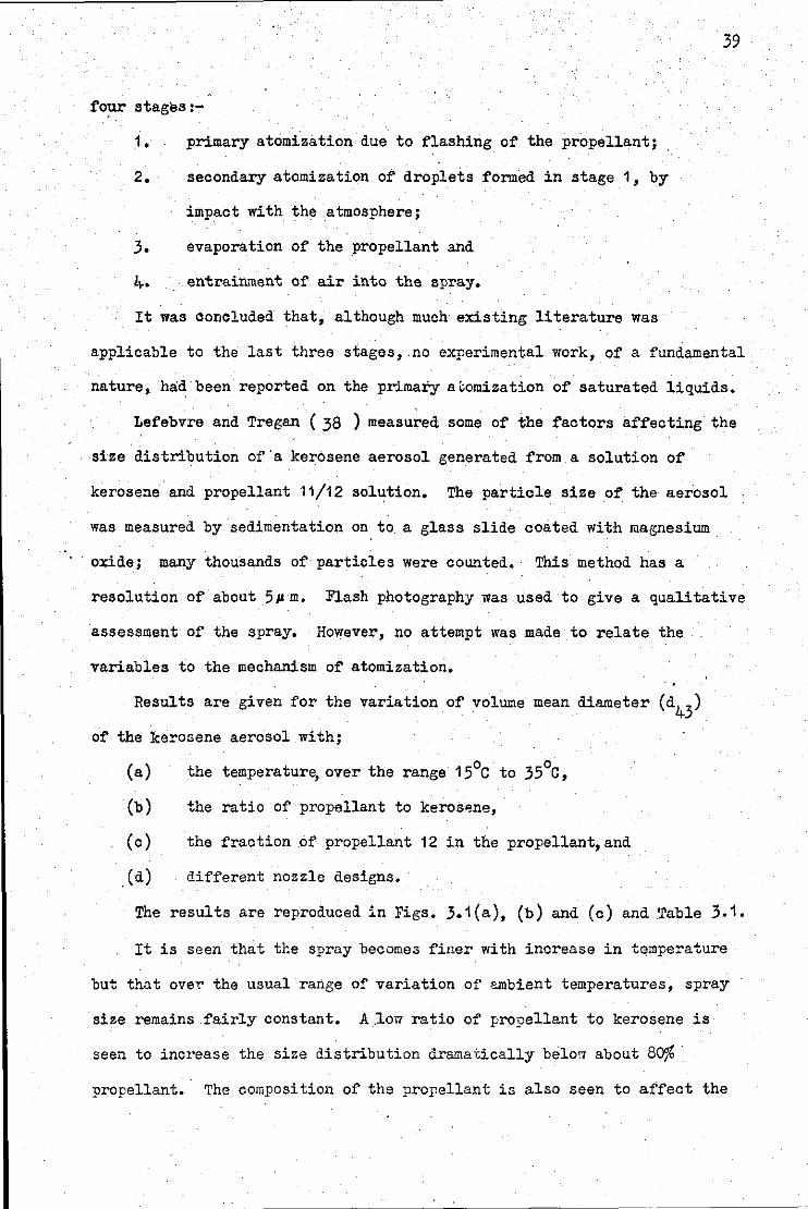
four stages:-
1, primary atomization due to flashing of the propellant;
2, · secondary atomization of droplets formed in stage 1, by
impact with the atmosphere;
3, evaporation of the propellant and
4. entra~~ent of air into the spray,
It was concluded that, although much existing literature was
applicable to the last three stages, .no experimental work, of a fundamental
nature, had been reported on the primary a i;omization of saturated liquids,
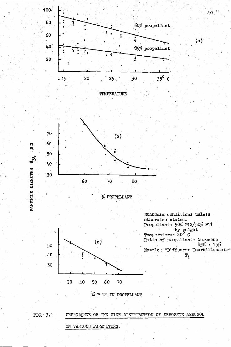
Lefebvre and Tregan ( 38 ) measured some of the factors affecting the
size distribution of'a kerosene aerosol generated from a solution of
kerosene and propellant 11/12 solution, The particle size of the aerosol
was measured by sedimentation on to a glass slide coated with magnesium
oxide; many thousands of particles were counted. This method has a
resolution of about Spm, Flash photography was used to give a qualitative
assessment of the spray, However, no attempt was made to relate the
variables to the mechanism of atomization, .. Results are given for the variation of volume mean diameter (d
43)
of the kerosene aerosol with;
(a)
(b)
(c)
(d)
0 0 the temperatur~ over the range 15 C to 35 C,
the ratio of propellant to kerosene,
the fraction of propellant 12 in the propellant,and
different nozzle designs,
The results are reproduced in Figs. 3.1(a), (b) and.(c) and Table 3.1.
It is seen that the spray becomes finer with increase in temperature
but that ove~ the usual range of variation of ~bient temperatures, spray
size remains fairly constant. A.low ratio of pro9ellant to kerosene is
seen to increase the size distribution dramai;ically below about 80%
propellant. The composition of the propellant is also seen to affect the
a ... -:I-
""!<'\ P:: ~
§ l=l
~ <.> H 8
~
100
80
60
4-0
20
70
60
50
40
30
50
40
30
FIG. 3,1
• •
• • •
• 4-0
60% propellant •
• • • \ (a) • • •
. 85% propellant • ' • ': • . ~
I • •
20 25 30
TEMPERATURE
60 70 80
% PROPELLANT
30 40 50 60 70
% P 12 IN PROPELLANT
Standard conditions unless otherwise stated, Propellant: 50% P12/50% P11
by )jeight Temperature: 20 C Ratio of propellant: kerosene
85% : 15% Nozzle: "Diff'useur Tourbillonnair"
T1
DEPY!WENCE OF Tlill SIZE DISTP.IBUTION OF KEROSENE AEROSOL
ON VARIOUS P.'\PJJrETERS.
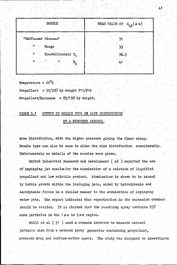
NOZZLE ..
"Di!'I'us~r Pinceau"
If Nuage
n Tourbillonnair T1 tt -· " T2
.
Temperature = 20°c
Propellant = 50/50% by weight P11/P12
Propellant/Kerosene = 85/15%by weight.
...
MEAU VALUE OF
71
35
36.5
41
TABLE 3.1 EFFECT OF NOZZLE TYPE ON SIZE DISTRIBUTION
OF A KEROSENE AEROSOL.
d43(J.I m)
size distribution, with the higher pressure giving the finer spray.
41
Nozzle type can also be seen to alter the size distribution considerably.
Unfortunately no details of the nozzles were given.
Oxford Industrial Research and Development ( 48 ) reported the use
of impinging jet nozzlesfor the atomization of a solution of liquified
propellant and low volatile product. Atomization is shown to be caused
by bubble growth within the impinging jets, aided by hydrodynamic and
aerodynamic forces in a similar manner to the atomization of impinging
water jets. The report indicates that vaporization in the expansion chamber
should be avoided. It is claimed that the resulting spray contains 25%
more particl~s in the 1 J.l m to 51J m region.
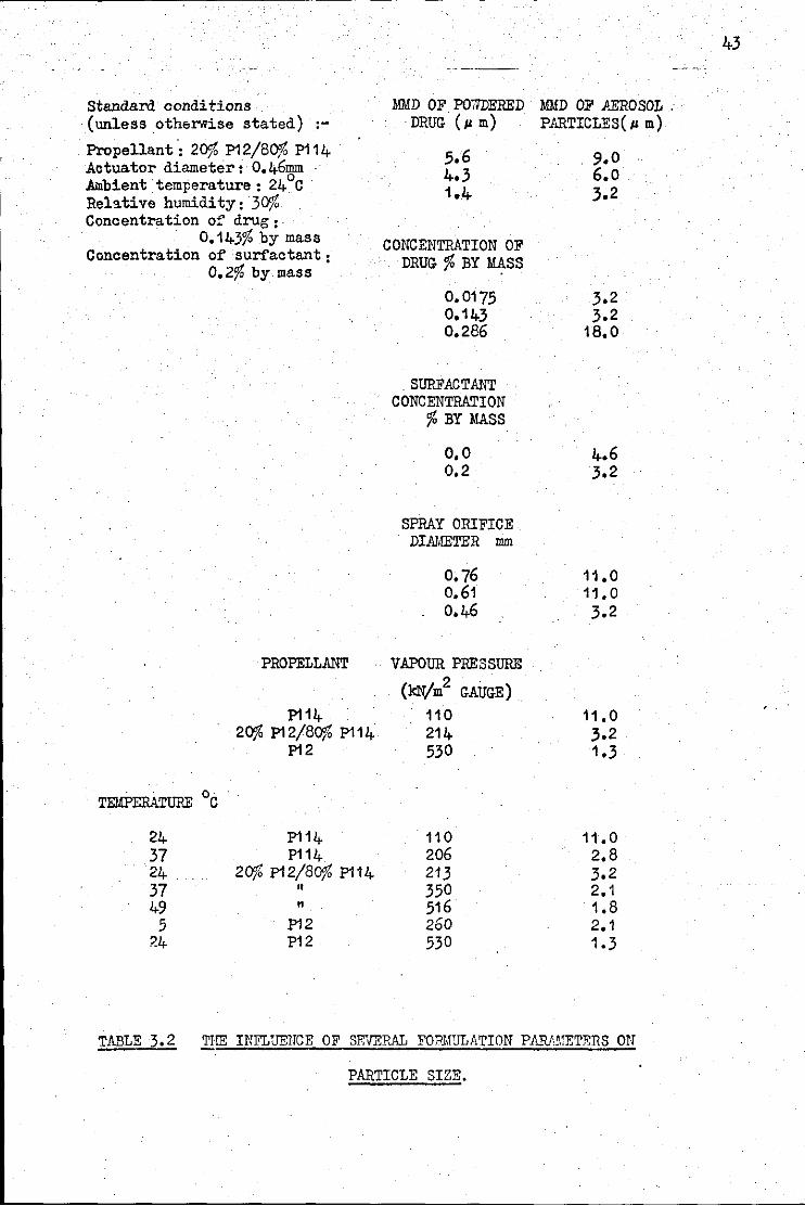
Polli et al ( 51 ) used a cascade impactor to measure aerosol .
particle size from a metered spray generatox' containing propellant,
powdered drug and surface-active agent. The study was designed to investigate
the influence ·or several. formulation parameters on aerosol particle
size. The results are shown in Tables 3.;2 overleaf.
From Table 3.2 it is seen that the size distribution and
concentration of the drug was found to have a marked effect on the aerosol size
distribution; but that the surfactant concentration had minimal effect.
Spray orifice diameter was found to have a marked effect, for diameters
below about o.6mm. · The effects or vapour pressure and temperature were
found to be similar to those found by Lefebvre and Tregan. A rise in
temperature of about 20 deg.C from nominal room temperature was found
roughly to halve the appropriate mean diameter·of the spray. Similarly,
doubling of the gauge pressure of the p~pellant was found
roughly to halve the mean diameter; at pressures below about 140 kN/m2
gauge however, the aerosol diameter was fou.~d again by both authors to
increase rapidly. Polli found that high pressure of about 520 kN/m2
gauge was required. for an aerosol size of the same order as that of the
original drug.
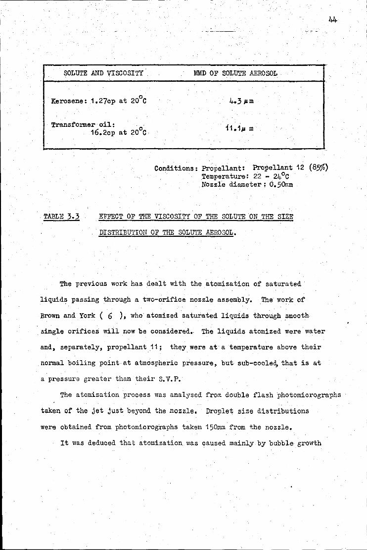
Tsetlin ( 67 ) measured the size distributions of kerosene and
oil aerosols generated by a continuous spray. The aerosols were
collected by sedimentation on to glass slides and mass mediam diameters
were measured by microscope counting. It was found that the M.M.D. was
reduced by increasing the proportion of propellant and by increasing
the temperature; this was in general agreement with the result of Tregan and
Lefebvre, and Polli. Table 3.3 shows that the M.M.D. of the oil aerosol
was considerable gr~ater than that of the Qil. This was attributed to
the higher value of the viscosity of the oil (16.2cp) compared with that
of the kerosene (1.27cp)
Standard conditions (unless otherwise stated)
Propellant·= 20% P12/80% P114 Actuator diameter: 0.46mm .Alnbient temperature : 24 °C Relative humidity: 30% Concentration of drug:·
0.143% by mass Concentration of surfactant:
o.z% by mass
24 37 24 37 49
5 ?.4
PROPELLANT
P114 20% P12/80% P114
P12
P114 P114
20% P12/80% P114 " n
P12 P12
MMD. OF P07lDERED Ml.!D OF AEROSOL . DRUG ( Jl m) PARTICLES( p m)
CONCENTRATION OF DRUG % BY MASS
0,0175 0.143 0.286
SURFACTANT CONCENTRATION
%BY MASS
0,0 0,2
SPRAY ORIFICE DIAMETER mm
0.76 0.61 0.46
VAPOUR PRESSURE
(kN/m2 GAUGE) .
110 214 530
110 206 213 350 516 260 530
9.0 6.0 3.2
3.2 3.2
18.0
11.0 11.0 3.2
11.0 2.8 3.2 2,1 1.8 2.1 1.3
TABLE 3. 2 :!,1lE INFLUENCE OF SEVERAL FOll.MULATION PA.lVJ,!ETERS ON
PA..ltTICLE SIZE.
43
SOLUTE AND VISCOSITY
0 Kerosene: 1.27cp at 20 C
Transformer oil: 0 16.2cp at 20 C
MMD OF SOLUTE AEROSOL
11.1p m
Conditions: Propellant: Propellant 12 (85%) Temperature: 22 - 24°C Nozzle diameter; 0.50mm
TABLE 3.3 EFFECT OF THE VISCOSITY OF THE SOLUTE ON THE SIZE
DISTRIBUTION OF THE SOLUTE AEROSOL,
The previous work has dealt with the atomization of saturated·
liquids passing through a two-orifice nozzle assembly, The work of
Brown and York ( 6 ), who atomized saturated liquids throl!gh smooth
single orifices will now be considered.. The liquids atomized were water
and, separately, propellant .11; they were at a temperature above their
normal boiling point at atmospheric pressure, but sub-coole~ that is at
a pressure greater than their S.V.P.
The atomization process was analysed from double flash ·photomicrographs
taken of the jet just beyond the nozzle. Droplet size distributions
were obtained from photomicrographs taken 150mm from the nozzle,
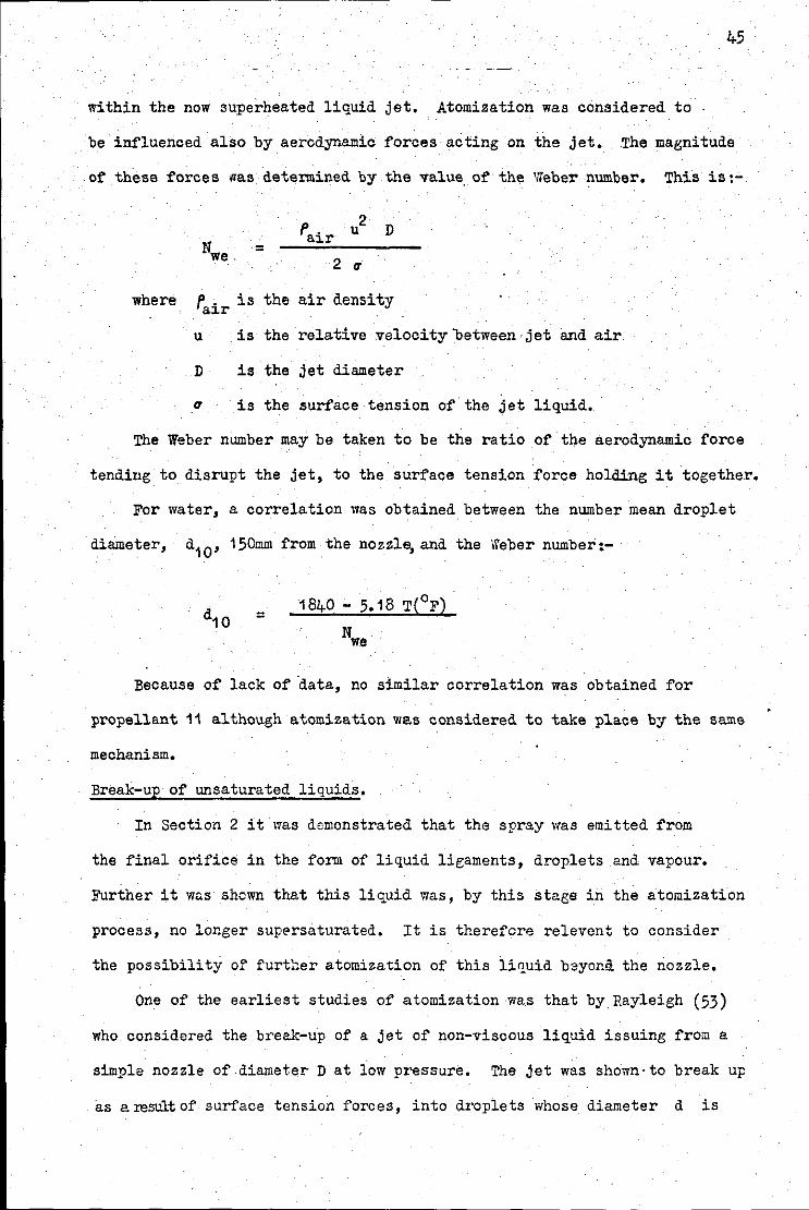
It was deduced that atomization. was caused mainly by bubble growth
,...----------------------------------------------
45
within the now superheated liquid jet. Atomization was considered to .
be influenced also by aerodynamic forces acting on the jet. .The magnitude
of these forces nas determined by the value. of the Weber number. This is:-
f' u2
D air =
2 tr
where f'. . is the air density aJ.r
u is the relative velocitybetween·jet and air
D is the jet diameter
(T is the surface tension of the jet liquid.
The Weber number may be taken to be the ratio of the aerodynamic force
tending to disrupt the jet, to the surface tension force holding it together.
For water, a correlation was obtained between the number mean droplet
diameter, d10 , 150mm from the nozzle, and the Weber number:-
= 1840- 5.18 T(°F)
Nwe
Because of lack of data, no similar correlation was obtained for
propellant 11 although atomization was considered to take place by the same
mechanism.
Break-up of unsaturated liquids.
In Section 2 it 1vas demonstrated that the spray was emitted from
the final orifice in the form of liquid ligaments, droplets and vapour.
Further it was shown that this liquid was, by this stage in the atomization
process, no longer sup~rsaturated. It is therefore relevent to consider
the possibility of further atomization of this liquid bayond the nozzle.
One of the earliest studies of atomization was that by Rayleigh (53)
who considered the break-up of a jet of non-viscous liquid issuing from a
simple nozzle of.diameter D at low pressure. The jet was shown·to break up
as a result of surface tension forces, into droplets whose diameter d is
given by·:-
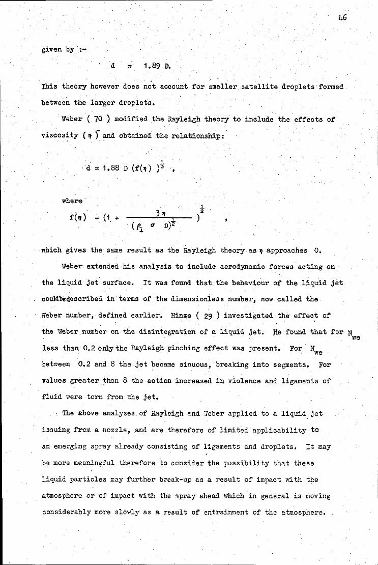
d = 1,89 D.
. This theory however does not account for smaller satellite droplets formed
between the larger droplets.
Weber (. 70 ) modified the Rayleigh theory to include the effects of
viscosity ( Jt ) and obtained the relationship:
d = 1,88 D (f(~) )'~ '
where t
) '
which gives the same result as the Rayleigh theory as~ approaches 0,
Weber extended his analysis to include aerodynamic forces acting on
the liquid jet surface. It was found that. the behaviour of the liquid jet
couldbedescribed in terms of the dimensior.less number, now called the
Weber number, defined earlier. Hin~e ( 29 ) investigated the effec: of
the Weber number on the disintegration of a liquid jet. He found that for Nwe
less than 0.2 only the Rayleigh pinching effect was present. For N we
between 0,2 and 8 the jet be.came sinuous, breaking into segments. For
values greater than 8 the action increased in violence and ligaments of
fluid were torn from the jet.
The above analyses of Rayleigh e.nd \'/eber applied to a liquid jet
issuing from a nozzle, and are therefore of limited applicability to
an emerging spray already consisting of ligamentn and droplets. It may
be more meaningful therefore to consider the possibility that these
liquid particles mo.y further break-up as a result of impact with the
atmosphere or of impact with the >'~pray ahead which in general is moving
considerably more slowly as a result of entrainment of the atmosphere.
This further break-up is called secondary atomization, Criteria. for
secondary· atomization have been determined by a number of people, All
.have found that secondary. atomization occured if a. critical value of the
Weber number was exceeded. Thus Lane (36), from experimental work with
water droplets in air at high Reynolds number, derived a value. for the
critical Weber. number of 4.1 for sudden application of the air stream~,
and 5, 7 for steady application. Haas ( 27 ) gives a. value of 5.6 from a
study of mercury droplets suddenly exposed to high velocity air stream,
Gordon ( 22 ) on theoretical grounds gives a. value of 8, The implication
of this criterion is considered later,
A vast amount of literature on atomization exists. It is mainly
related to pressure atomization and pneumatic atomization of unsaturated
li~uids, The former bears little resemblance to the atomization of
47
saturated liquids, The latter however·may have some bearing on the later
stages of saturated liquid atomization, This is because the propellant
vapour could in some circumstances be instrumental in the atomization of
the liquid propellant, It .is useful, however, to compare these two methods
with two-orifice saturated liquid atomization, Tr.is comparison is readily
made from an extensive review of both pressure and pneumatic atomization
by Dombrowski and Munday ( 11 ), An estimate of the volume-surface mean
diameter d32
of a saturated liquid spray in the vicinity of the nozzle
may be obtained from the size distribution of ita residual aerosol by
dividing by the cube root of the solute concentration, This assumes no
coagulation of the spray, Application of this to the results of Polli,
given earlier, produces a value of d32
of about 25 pm for the smaller
orifices, Data given in Section 6 yield similar results. Pressure
atomization of water from a swirl spray nozzle at the same pressure, of the
order of 350 kN/i gauge, at approximately the same flovr-rate, of the order
of 1 gm/sec (obtained again from Section 6 ), is shown, from the above review
48
· to produce a. mean diameter d32
of about 100 pm, As would be expected
pressure atomization·is considerably the less efficient. Prefilming pneumatic
atomization would produce a mean diameter similar to that of a saturated
liquid spray if the ratio by mass of gas to liquid was 2:1. As a. typical
saturated liquid spray, of modest propellant pressure, emits propellant
as a two-phase fluid of the order of 1o1o vapour quality, it again follows
that two-orifice saturated liquid atomization is comparatively efficient.
Properties of gas jets and sprays.
The behaviour of the spray in the atmosphere may now be considered.
It was shown qualitatively in preliminary work that a metered spray was
turbulent and furthermore the total volume of the resultant spray was
considerably greater than the volume of propellant vapour; the spray
therefore consisted mainLy of entrained air. It is therefore relevant
to consider published work on turbulent air jets, the effect of loading
the jet with partioulate matter, and the entrainment of air into sprays.
The behaviour of gaseous jets is well unaerstood, Information on
such jets is well documented ( 49, 66 ) • This is considered in more detail
in the next section. The behaviour of particulate·matter .within a jet is
less well documented. Goldschmidt and Eskinazi ( 21 ) reviewed work on
diffusion of particulate matter in turbulent flow and presented a theory
for the diffusion of small particles in a plane air jet, Experimental
data were obtained which were compared w:i:th the theory; good agreement
was found, The data were obtained from measurements.of the concentration
flux and concentration of aerosol particles in the plane air jet. The
concentration of the aerosol was very low,however,of the order of 10-7 by volume
at the nozzle. It was found that the transverse distribution of concentration
flux and concentration beyond about 30 nozzle diameters were approximately
Gaussian. The axial distribution of concentration flux was inversely
proportional to the downstream distance frcm the apparent origin of the
..
spray, while the axial distribution o~ concentration was inversely proportional
to the square root o~· the distance •.
Laats ( 34 ) measured the e~~ect o~ loading an air jet with particulate
matter whose mass ~low-rate was o~ the order of that of the air. It was
~ound that the divergence o~ the jet was reduced slightly and hence the
attenuation o~ axial velocity was also slightly reduced.
Entrainment o~ air into jets may now be considered. Again for an
air jet the theory is well established. For sprays Mayer and Ranz (40)
presented a theoretical expression for entrainment o~ air, based on the
assumption of uniform velocity across the spray.
Brif~a and Dombrowski { 3 ) measured, indirectly, the ratio o~ air
entrainment into a flat spray obtained from the disintegration o~ a
liquid sheet. They compared the results with theory based on momentum
· conservation. Reasonable agreement between experiment and theory was
obtained. It was noted that their expression for the ratio of mass of
entrained air to the spray liquid was similar to the analogous expression
for an air jet. Benatt and Eisenklam { 1 ) made direct measurements
o~ the rate o~ entrainment o~ air into water sprays ~ram swirl nozzles,
using a porous pot technique. It was ~ound that the mass rate o~ entrainment
of air was approximately equal to that. into an air jet i~ the spray angle
was equal to that o~ the air jet.
.50
3.2 Particle size and velocity measurements.
It has been demonstrated in Section 1 that the spray parameters o~
interest are the size and velocity distributions o~ the particles within
the spray, and also the size distribution o~ the resultant aerosol o~ the
pharmaceutically active ingredient. Because in general, within the spray,
particle velocity varies with particle diameter, it is desirable, but not
necessarily essential, to measure spray-particle size and velocity
simultaneously.
In this sub-section methods o~ measurement o~ the size and velocity
o~ rapidly moving particles will be reviewed. Also method of particle
size measurement of the resultant aerosol will be summarised;
Double exposure photomicrography.
Double exposure photomicrography is. probably the simplest technique
for obtaining simultaneous size and velocity measurements of a pray particles.
It was used successfully by York and Stubbs ( 7.5 ) , and others ( .52 , 17)
for example. The usual design is a sub-microsecond spark as a light source.
and a high resolution lens arranged in the transmitted-light configuration.
With this arrangement rapidly moving particles of diameter about 41' m
may be resolved at speeds of the order of 40 m/sec;
Particles smaller. than 4Pm may be detected using dark field illumination,
but this technique is not readily applicable to spray photography because
of confusion caused by out-of-focus particles.
Rotating mirror photomicrographic system.·
Ingebo ( 30 , 31 ) used a rotating mirror in a otherwise conventional
photomicrographic system to measure the size and velocity distributions
of ethanol particles in a rocket combustor, Tne use of the rotating mirror
enabled rapidly moving particles to be photographed with a relatively long
duration (8 p. sec) spark light source. This duration was found necessary
in order to provide sufficient light. From the optimum speed of rotation
of the mirror, the speed· of the particles was determined; this ranged
from 10 to 20 m/sec.
Fluorescent Photography.
The transmitted-light photomicrography technique described above
51
gives good results providing a resolution limit of a few micrometres is
acceptable. It has the disadvantage however that automatic scanning
techniques for particle size analysis are not readily applicable ( 52 )
because of the presence.of out-of-focus particles. To eliminate the problem
of out-of-focus particles the illumination must be confined to a narrow sheet
in a. plane nonnal to the camera axis. Benson et al ( 2 ) tested this
technique. They found that the intensity of the scattered light was low and
that the particles were unevenly illuminated; highlights were created on
one side of the particle, making size measurements difficult. These problems
were overcome by dissolving an ultra-violet absorbing fluorescent dye into
the spray-generating liquid, for example uranin in water. The spray droplets
then became luminous, and as the induction and decay times of the dye were
very short, of the order of 5 nsec, the droplets remained in focus while
still emitting light. Consequently all droplets photographed_ were in focus
and there was no bright background to reduce the contrast of the images of
smaller particles.
Groeneweg et al ( 26 ) modified this technique by using a "Q"-svdtched
ruby laser in a frequency doubling mode such that a 50 nsec pulse of ultra
violet (347 nm) was obtained. The authors state that with this system,
resolved images of 10 JJ m particles travelling at 50 m/sec could be obtained.
The lower limit of resolution is not given, b~t there seems no theoretical
reason why smaller particles should not be photographed in this way. Further,
the use of a double-pulsed laser system would eno.ble velocities to be measured.
Holography
Fraunhofer holography, as a means of particle size measurement was
developed in 1966(64,65,68,69) initially to obtain the size distribution
52
of' the water droplets in f'og. The resolution of' the system was about 31.1 m
and the overall depth of' field of the hologram was about 300mm. It was
possible however, on reconstruction of' the hologram to restrict the depth
of' field optically, and scan longitudinally through the total field of view.
In this way the number of' particles in focus in any one field could be
restricted to a convenient number. The experimental arrangement of a
single pulsed Fraunhof'er holographic system was described in Section 2.
More recently Fourney et al ( 18 ) developed a dOuble· pulsed holography
system with which size and velocity distributions of' particles could be
determined. Resolution was shown to be approximately 5 1.1m.
It is considered that holography is a useful technique for particle
size and velocity measurement, especially when a large depth of'. field is
required. However, as explained in Section 2, the technique could not be
applied to particles within a spray generated by a liquified gas because
of' loss of' coherence of' the laser beam as a· result of' its P!l.5Sage through
the propellant vapour, and a dense field of' particles.
The techniques so far discussed have been applicable to the detexmination
of' size and velocity distribution of' rapidly moving particles. The
determination of' the size distribution of' the residual aerosol may now be
considered.
A large number of techniques are available for the determination of'
the size distribution of aerosols. However, as discussed in Section 2, it
is necessary_that_the_system should have a resolution of' about 1 1.1 m or less
but not discriminate against particles of diameter up to about 501.1 m.
This will generally mean that no single method of size analysis is
applicable. This is because either the method of' sampling is discriminatory
or the applicable size range is less than that required. For· example the
terminal velocity of a 501.1 m particle is approximately 72 mm/sec. Thus
any aerosol sizing method ,·:hich relies en ~ampling from the aerosol will
53
inevitably discriminate against such particles. This disadvantage may be
over~ome by sampling twice, using two methods such that there is an overlap
with respect to the diameter of particles sampled efficiently. Thus, using
this principle Sch6nauer ( 58 ) for example, was able to measure the size
distribution of an azulene medical spray whose size distribution ranged
from approximately 0.1 pm to 30pm. The coarser fraction, above 1.7 pm
diameter, was sampled by sedimentation for 10 hours and analysed with an
optical microscope, The finer fraction below 2. 3 pm, was sampled with
a thermal precipitator and analysed using an electron microscope using a
standard replication technique together with knowledge of the "flattening
factor" of the original flattened droplet on the electron microscope grid.
The two distributions were readily combined to give the complete distribution.
Having thus eliminated the problem of the larger size fractions, a
number of sizing techniques for the smaller fraction is available. For
example, in addition to electron micrography mentioned above, the principle
of light scattenng from individual particles may be employed,using commercially
available instruments (55 ),to determine particle size in 'the range 0.3 to
10 pm. Alternatively an electrical particle analyser ( 71 ) may be used
to measure the size distribution of )?articles in the range 0. 015 to 1.2 I' m.
Centrifugal sedimentation may be used to classify particles according to
diameter. Compared with gravitational sedimentation, centrifugal deposition of
sub-micron particles is quicker and more effective. An early device, the "conifuge"
( 56 ) graded particles in the size range 30 to 0. 5 pm. A later version,
the "aerosol spectrometer" ( 20 ) , was applicable to particles in the size
range 3 to 0.03 pm. Cascade impactors have been shown to classify particles
succe~sfully. An early four-stage version ( 39 ) had a lower deposition
limit of approximately 0. 7 pm. A later six-stage version. (43) extended the lower
limit to 0.3 Pm. The upper limit in this case is .determined by wall losses at
the first orifice and, as before, sampling efficiency cf large particles
from an aerosol. \7all losses were considered to become serious with
particles· above 50 pm.
55
).) Flow o~ s~tur~ted liquids and two-phase ~luids through
nozzles.
·The ~low of saturated propellant through a two-ori~ice nozzle assembly
of the type used in this work may be divided into two parts. The first
is the flow through the ~irst, upstream, ori~ioe (short tube) when the
propellant is ~ liquid ~arm on entering the ori~ice. The second part is
~low through the second ori~ice. In this case the propellant is in the
form o~ an intimately dispersed two-phase ~luid - the liquid propellant
and its vapour. It is therefore releve:ht to review literature relating
to these two types of flow.
3.3.1 The flow o~ a saturated liquid through an expansion device.
Early work on nozzle ~low o~ saturated fluids, both liquids and
vapours, assumed thermodynamic equilibrium throughout the_~low• Thus
saturated liquids were ass_umed to vaporise instantly on entering the
nozzle as a result of the reduction in pressure, and vapours in general
were assumed to condense. Using this model in which thermodynamic
equilibrium was assumed,. it was ~ound that actual mass ~low-rates were
greater than the predicted values. Thus Stuart and Yarnell ( 61 ), ~or
example, predicted mass flow-rates o~ saturated water through a two-
orifice nozzle. They then compared their predictions ( 62) with
experimentally dete1~ined values. It was ~ound that the experimental
values were considerably higher than predicted. For example the ~low-
rate of saturated water at 690 kN/m2 abs -;;as predicted to be 2.3 x 10³ kg/m2/sec
while the measured rate was 7.2 x 10³ kg/m2fsec. The discrepancy was
attributed to the existe!lce o~ a metastable state, in which pressures were
generally lower than the saturation levels. A further calculation was
therefore performed in which metastability was included; it was assumed
that there was no vaporisation during passage through the first orifice
and that there was no change in vapour quality (mass fraction vaporised)
during passage through the second orifice. It was further assumed that
there was no change of specific volume or temperature through the second .
orifice. The ·predicted mass flow-rate, again for a saturation pressure
of 690 kN/m2, was 12 x 103 kg/m2jsec giving a discharge coefficient of·
0,61 for the second, downstream, orifice. This, the authors considered
acceptable. It would seem however that the assumption of constant specific
volume .through the second orifice was physically unrealistic; indeed it
would result in adiabatic flow of deoreasillg entropy.
Pasqua ( 50 ) studied the flow of refrigerant (or propellant) 12, ·
through orifices, short tubes and nozzles. For saturated 'liquid flow through
orifices complete metastability was found, and the usual orifice formula
could be used to predict the flew-rate.
For saturated liquid flow through short tubes it was found that the
liquid immediately broke away from the wall of the tube and was surrounded
by an annulus of vapour; the tube then displayed orifice characteristics
as above. Below a critical downstream pressure the flow became mass limiting.
This critical pressure
p = 0.37 c
p0
was given by :-
L 0.2 (D) x (initial saturation pressure),
where L/D is the ratio of the length to diameter of the short tube.
For sub-cooled liquid flowing through short tubes, full tube flow
was observed until the pressure fall rcsul·ted in a pressure at the vena
contracta equal to the S.V.P. of the liquid; the flow then reverted to
orifice flow as before.
For nozzle flow of ·saturated ·liquid, it was found again that the flow
broke from the tube and a vapour ~ulus was formed. ~be flow could be
57
predicted by the conventional nozzle equation providing a coefficient of
contraction was introduced, which was based on the length-to-diameter ratio
of the nozzle.
Fauske and Min ( 16 ) studied the :f'low of' saturated propellant 11
through apertures and short tubes. Similar results to those of' Pasqua
were found. ~us f'or f'low through apertures, the saturated liquid was
found to behave as an unsaturated liquid. Short tubes behaved as apertures,
with a discharge coefficient of 0.61, providing critical conditions were
not reached. The critical point was defin~i in terms of' a modified cavitation
number:~
'
where 6 P is the pressure difference across the tube, A is the
tube area, rl is the liquid density and Q is the volume flow-rate.
L/D is again the length-to-diam~ter ratio of the tube.
Flow remained non-critical below a modified cavitation number .of' 1 O.
Above a value of' 14 the flow became critical or mass limiting. Between
10 and 14 there was a transition region in which both types of' f'low could
tske place.
3.3.2 The flow of two-phase fluid through an expansion device.
A vast amount of' literature exists on two-phase flow. This is a
result of r.ork conducted mainly in connection with atomic power generation,
in particular with the prediction of the rate of escape of coolant in the
event of damage to the cooling system. Because of this, most of the work
has be~n done on flovr through pipes. One of the earliest reports of two-
phase flow through nozzles, however, was that of Tangren et al ( 63 ) who
58
studied the flow of an air/water mixture through de Laval and convergent
nozzles. · A theoretical treatment, was given. In this it was assumed that
choking effects, analogous to those in single phase compressible flow,
would be present for values of. the ratio of downstream to upstream pressure
below a critical value, Under conditions of choking it was assumed that
the velocity oi' the fluid at the throat of a nozzle would be equal to the
velocity of a pressure pulse through the fluid, On the basis of these
. assumptions the above critical pressure ratio was calculated for a number
of values of' the ·ratio of air to water.· These were then compared with
experimentally determined values. It was found that the measured critical
pressure ratios varied from about 0.43 to 0,60 for initial values of the
ratio by volume of air to water of 0.19 to 2.0. Predicted values of the
pressure ratio were in error by no more than 13%.
The work of Tangren and other studies of single nozzle and twin-
orifice nozzle assemblies were reviewed in a comprehensive survey by
Smith in 1963 ( 59 ). The author of this survey recommended that for
two-phase flow of' low quality through short expansion devices,wluch is the
type of flow to be expected through the.downstream orifice of' the twin
orifice spray generator of the present work, a homogeneous metastable flow
model. should be used. This was the model used by Tangren.
Edmonds and Smith ( 12 ) studied mass limiting two-phase flow of
propellant 11 in a long nozzle, a short nozzle and also a straight tube.
Measurement_of_mass_flow-rate_and exit plane pressure were made for a
constant initial pressure at different values of vapour quality and receiver
pressure. It was found that as the receiver pressure was lowered, the
pressure at the exit plane of the three devices became constant, but only
when the receiver pressure was lower than the exi·t plane pressure by a
substantial margin. In the case of the straight tube this margin was
30 kN/m2 ; for the long nozzle the margin was about 60 kN/m2 and for the
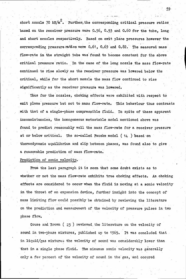
59
. ·~ 2 short nozzle 70 kN1 m • Further,the corresponding critical pressure ratios.
based on the receiver pressure were 0.56, 0.53 and 0,60 for the tube, long
and short nozzles respectively. Based on exit plane pressures however the
corresponding pressure ratios were 0,61, 0.69 and 0,82. The measured mass
flow-rate in the straight tube was. found to become constant for the above
critical pressure ratio. In the case cf .the long nozzle the mass flow-rate
continued to rise slowly as the receiver pressure vras lowered below the
critical, while for the short nozzle the mass flow continued .to rise
significantly as the receiver pressure was lowered,
Thus for the nozzles, choking effects were exhibited with respect to
exit plane pressure but not to mass flow-rate,
.with that of a single-phase compressible fluid.
This behaviour thus contrasts
In spite of these apparent
inconsistancies, the homogeneous metastable model mentioned above was
found to predict reasonably well the mass flow-rate for a receiver pressure
at or below critical. The so-called Fauske model ( 14 ) based on
thermodynamic equilibrium and slip between phases, was found also to give
a reasonable prediction of mass flow-rate.
Prediction of sonic velocity.
From the last paragraph it is seen that some doubt exists as to
whether or not the mass flow-rate exhibits true choking effects. As choking
effects are considered to occur when the fluid is moving at a sonic velocity
in the throat of an expansion device, further insight into the concept of
mass limiting flow could possibly be obtained by reviewing the literature
on the prediction and measurement of the velocity of pressure pulses in two
phase flow,
Gouse and Brovm ( 23 ) reviewed. the literature on the velocity of
sound in two-phase mixtures, published up to 1965. It was concluded that
in liquid/gas mixtures the velocity of sound was considerably lower than
that in a single phase fluid. The minumum sonic velocity was generally
only a few percent of the velocity of sound in the gas, and occured
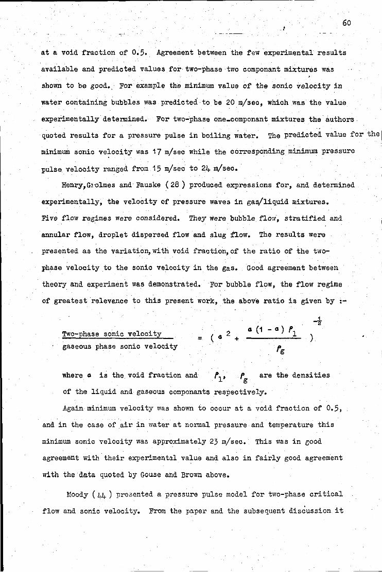
60 I
at a void fraction of 0.5. Agreement between the few experimental results
available and predicted values for two-phase two component mixtures was
shown to be good •. For example the minimum value of the sonic velocity in
water containing bubbles was predicted to be 20 m/sec, which was the value
experimentally determined. For two-phase one-component mixtures the authors
q,uoted results for a pressure pulse in boiling water. The predicted value for the I
minimum sonic velocity was 17 m/sec while the corresponding minimum pressure
pulse velocity ranged from 15 m/sec to 24 m/sec.
Henry,Gl·olmes and Fauske ( 28 ) produced expressions for, and determined
experimentally, the velocity of pressure waves in gas/liq,uid mixtures.
Five flow regimes were considered. They were bubble flo:v, stratified and
annular flow, droplet dispersed flow and slug flow. The results were
presented as the variation, with void fraction, of the ra tic of the two
phase velocity to the sonic velocity in the gas. Good agreement between
theory and experiment was demonstrated. For bubble flow, the flow regime
of greatest relevance to this present work, the abov·e ratio is given by ·-
Two-phase sonic velocity
gaseous phase sonic velocity
where o is the void fraction and
= ( 0 2 +
-t )
are the densities
of the liq,uid and gaseous components respectively.
Again minimum velocity was shown to occur at a void fraction of 0.5,
and in the case of' .air in water at normal pressure and temperature this
minimum sonic velocity was approximately 23 m/sec. This was in good
agreement with their experimental value and also in fairly good agreement
with the data q,uoted by Gouse and Brown above.
Moody ( L.4) presented a :Pressure pulse model for two-phase critical
flow and sonic velocity. From the paper and the subsequent discussion it
was concluded that, as demonstrated by the previous paper, the sonic
velocity in a two-phase. mixture was readily predictable. However doubt
exists as to the predictability of cri ticai velocity owing to difficulty
in ass.essing conditions at the point of choking.
L__ ___________________ ._
61

62
3.4 Conclusions from the literature.
It is apparent from a survey of the literature that fairly adequate
empirical descriptions of the size distributions of pressure atomized and
pneumatically atomized sprays were available. A theoretical basis for these
descriptions however was generally lacking, although the primary break-up
mechanisms appear to be reasonably well understood. In the case of
atomization of saturated liquids, well established empirical relationships
are lacking, although trends of variation of particle size distribution
with such factors as temperature, propellant pressure and concentration,
and the concentration and viscosity of the solute are available, although
little attempt has been made to explain these trends theoretically.
One aspect of the theoretical.treatment of pressure and pneumatic
atomization can be applied directly ·to atomization of saturated liqUids.
This is ·the criterion of secondary atomization which may be applied to
determine the maximum droplet size in a spray. This criterion was shown
to be. that the droplets would further break up if the 'v1eber number exceeded
a value of about 5 for sudden application.of the disrupting force. The
Weber number for a particle diameter, d
2 u d tT
, is given by :-
•
For a pure, solute free, propellant the surface tension is about
12 x 10-3 N/m (12 dynes/cm). Assuming injection at 30 m/sec (from Section 6)
into still air = then:-
= > 5 '
or d > 100 pm.
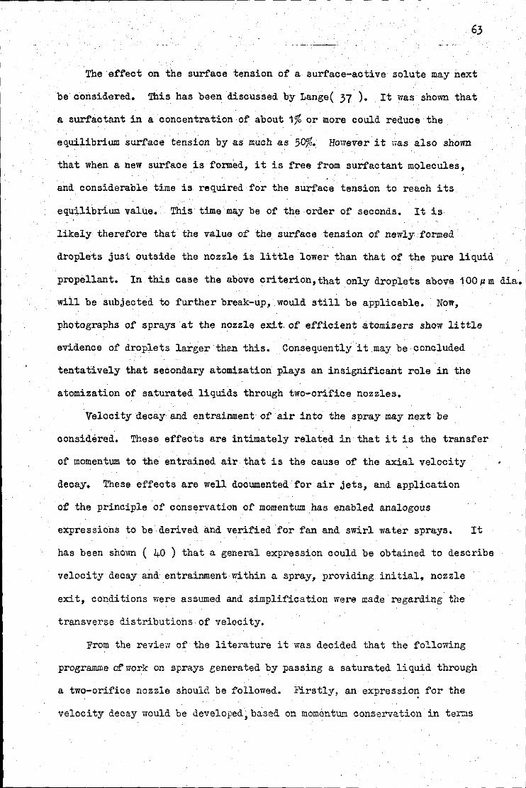
63
The effect on the surface tension of a surface-active solute may next
be considered. This has been discussed by Lange( 37 ). It was shown that
a surfactant in a concentration of about 1% or more could reduce the
equilibrium surface tension by as much as 50%. However it 1¥as also shown
that when a new surface is formed, it is free from surfactant molecules,
and considerable time is required for the surface tension to reach its
equilibrium value. This time may be of the-order of seconds. It is
likely therefore that the value of the surface tension of newly formed
droplets just outside the nozzle is little lower than that of the pure liquid
propellant. In this case the above criterion,that only droplets above 100pm dia.
will be subjected to further break-up, would still be applicable. Now,
photographs of sprays at the nozzle exit. of efficient atomizers show little
evidence of droplets larger than this. Consequently it may be concluded
tentatively that secondary atomization plays an insignificant role in the
atomization of saturated liquids through two-orifice nozzles.
Velocity decay and entrainment of air into the spray may next be
considered. These effects are intimately related in that it is the transfer
of momentum to the entrained air that is the cause of the axial velocity
decay. These effects are well documented for air jets, and application
of the principle of conservation of momentum,has enabled analogous
expressions to be derived and verified for fan and swirl water sprays. It
has been shown ( 40 ) that a general expression could be obtained to describe
velocity decay-and-entrainment within a spray, providing initial. nozzle
exit, conditions were assumed and simplification were made regarding the
transverse distributions of velocity.
From the re·;ie;·1 of the literature it was decided that the following
programme afwork on sprays generated by passing a saturated liquid through
a two-orifice nozzle should be followed. Firstly, an expressiot; for the
velocity decay would be developed, based on momentum conservation in tel"tls
L-------------------------------~--------------------------
64
of the fundamental parameters of the system, The initial momentum of the
spray, given in terms of mass flow-rate and initial spray velocity, would
be determi.~ed from the assumption of homogeneous metastable flow through
the downstream orifice. The validity of these. predictions would be
assessed experimentally from measurements of pressure,temperature and
mass flow-rate of the propellant, and also from size and velocity data of
the spray; the latter would be obtained from double-exposure photomicrography.
The second part of the programme would be an attempt to extend or
consolidate e.~sting knowledge regarding size distributions from such sprays;
if possible this information on the size distribution would be again
related to fundamental parameters of the system.
65
4 THEORY
Introduction
4.1 Axial distribution of the mean velocity within a spray.
4.2 Flow of a saturated liquid through a two-orifice nozzle.
Introduction
The formation of an aerosol spray by the passage of a saturated liquid
through a two-orifice* nozzle assembly may be summarised as follows.
Initially the propellant in the liquid phase, passes through the upstream
orifice into the low pressure region of the expansion chamber. There flash
evaporation creates a turbulent mixture of vapour and liquid ligaments.
This two-phase fluid" then discharges from the downstream orifice in the
form· of a turbulent jet, consisting of fine ligaments, droplets a.~d vapour.
The surrounding air is entrained, by turbulent mixing, into the jet which
consequently diverges and slows down.
Within the jet, droplets initially formed at the exit of the
downstream orifice may break up further as a result of surface tension
forces or impact with the surrounding. air; coalescence of droplets may
also take place.
The final stage is the evaporation of the propellant. .!hen only
propellant is the spray-generating liquid, the result is a jet of' propellant
vapour and entrained air, In the case of a pharmaceutical spray whose
propellant conteins a solute or suspended powder, the jet also contains
an aerosol of fine solute or powder particles.
The spray properties of interest have been discussed in the first
seotion. There, it was shown that the properties.of the spray most
relevent to inhalation therapy were the velocity and size distribution of
the spray particles. It wan therefore considered desirable to be able to
"' They resemble "orifices" although , as described later, they are "short tubes",
66
predict these parameters theoretically.
It is apparent from the above description of spray formation that
both of these parameters involve a number of related physical phenomena
and that the theoretical description of either would be a multi-facet
problem. The prediction of spray velocity re~uires the knowledge of the
initial momentum of the spray together with the degree of entrainment of
the surrounding air. The prediction of size distribution within the spray
requires the prediction of the size distribution at the orifice together
with knowled~e of the degree of secondary atomization, coalescence and
evaporation within the spray •
.An investigation into the possibility of deriving a fundamental theory
to describe the above two parameters together with experience gained from
the preliminary vrork led to the following conclusions. The first was that
the description should be confined to a continuous spray only. The reasons
for this limitation were described in Section 2 where it was shown that
the discharge of a metered spray because of its transient nature was not
readily amenable to mathematical treatment, and would add undesirable
complexity to the problem. The second was that it seemed likely that the
various stages of the spray development, nozzle flow, jet development etc.
could be predicted and that by combining these a complete description of
the velocity profiles within the spray could be. obtained in terms of the
nozzle dimensions and the thermodynamic properties of the fluid with the
need for the minima of assumptions and empirical factors. The third
conclusion was that it would be unlikely that the particle size distribution
could be similarly described. This is based on. the experience reported by
many authors, who found that particle size distribution could only be
predicted empirically. Perhaps the best known example is that of Nukiyama
and Tanasawa ( 46) who produced empirical expressions for the size
distribution of pneumatically produced spr~ys. Consequently an empirical
67
approach was taken f'or this second part of' the work.
It is the purpose of this Section therefore to develop an expression
by means cf which the velocity within the spray. could be determined in terms
of' the fundamental properties of the system with resort to as f'ew assumptions
and empirical factors as possible. As transverse velocity profiles can
usually be assumed to be Gaussian, as discussed in the literature, only the
axial velocity profile need be considered. Thus, in the first part of.the
Section an expression f'or the axial velocity profile is developed in terms
of the initial momentum of the spray. In the second part the initial momentum
of' the spray is determined in terms of the fundamental properties of the
system. Therefore a relationship between these properties and the axial
velocity profiles is established.
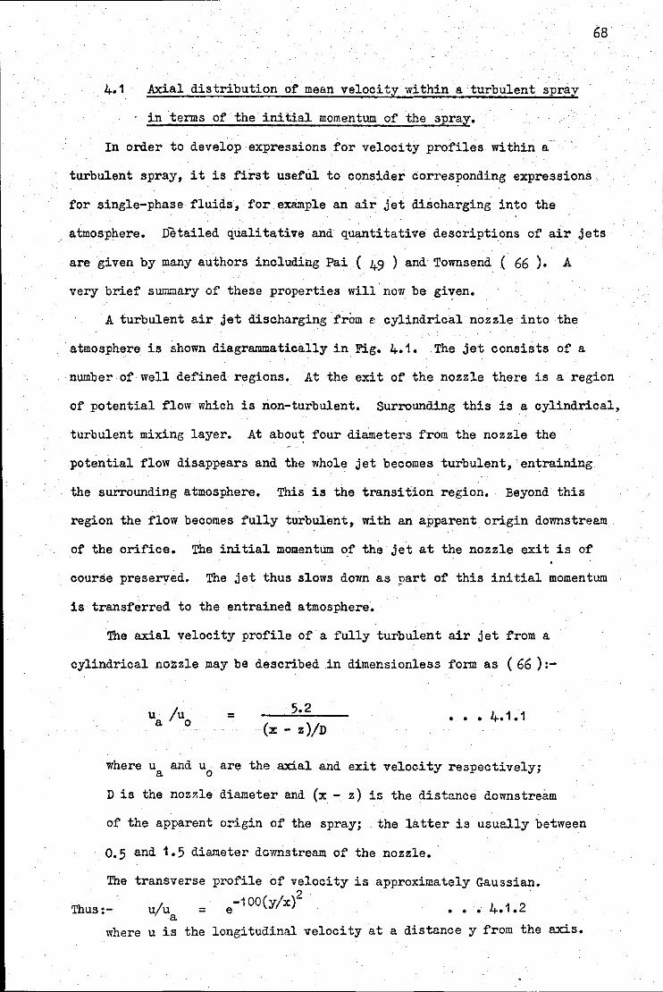
4,1 Axial distribution of mean velocity within a turbulent spray
in terms of the initial momentum of the spray.
In order to develop expressions for velocity profiles within a·
turbulent spray, it is first useful to consider corresponding expressions
for single-phase fluids, for example an air jet discharging into the
68
atmosphere. Detailed qualitative and quantitative descriptions of air jets
are given by many authors including Pai ( 49 ) and Townsend ( 66 ). A
very brief summary of these properties will now be given.
A turbulent air jet discharging from e cylindrical nozzle into the
atmosphere is shown diagrammatically in Fig. 4.1. The jet consists of a
number of well defined regions. At the exit of the nozzle there is a region
of potential flow which is non-turbulent. Surrounding this is a cylindrical,
turbulent mixing layer. At about four diameters from the nozzle the
potential flow disappears and the whole jet becomes turbulent, ·entraining
the surrounding atmosphere, This is the transition region, Beyond this
region the flow becomes fully turbulent, with an apparent origin downstream
of the orifice, The initial momentum of the jet at the nozzle exit is of
course preserved. The jet thus slows down as part of this initial momentum
is transferred to the entrained atmosphere,
The axial velocity profile of a fully turbulent air jet from a
cylindrical nozzle may be described .in dimensionless form as ( 66 ) :-
= 5.2 • • • 4.1.1 (x - z)/D
where u and u are the axial and exit velocity respectively; a o
D is the nozzle diameter and (x - z) is the distance downstream
of the apparent origin of the spray; . the latter is usually between
0.5 and 1.5 diameter downstream of the nozzle.
The transverse profile of velocity is approximately Gaussian. 2
Thus:- u/ua = -100(y/x) .; 4.1.2 e • •
where u is the longitudinal velocity at a distance y from the axis.
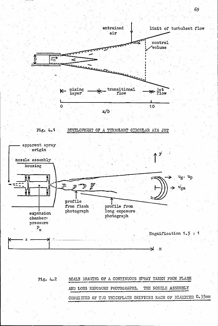
-
r
I lK D
... ---- ... lu~ : 0
"' ............. -
Fig. 4.1
apparent spray origin
nozzle assembly housing \
0
entrained air
--- _ .... --;;.:- ... --' ------, ..,.,. < .... .... ....... -- .....
mixing layer
--- -----'""':::-----
-----l)r(!-- transitional flow
x/D
69
limit of turbulent flow
control
. t * H.ow
10
DEVELOPMENT OF A TURBULENT CIRCULAR AIR JET
iy
-~------- ........
M ~ . ~ - . = !5' .:..-~· ~. __,. ~~#~ ~ ,..
i --~-r=~. -:-----:=·· ~
z
expansion chamber: pressure
pe
I
Fig, 4,2
profil~ . from flash profile from photograph long exposure
photograph
Magnification 1.5 1
X
SCALE DRA\'IING OF A CONTINUOUS SPRAY TAKEN FROM FLASH ··-AND LONG EXPOSURE PHOTOGP.APHS. THE NOZZLE ASSEMBLY
CONSISTED OF T'JO THICKPLATE ORIFICES EACH OF DlAl.lE'rER 0.35mm
It follows from this equation that the divergence angle of the jet
corresponding to the 1/e - velocity locus is :-.
0 or 5.8
It also follows that the dimensionless transverse profile is independent
70
of the distance downstream •. This applies also to other properties of the
jet, which is thus self-preserving.
The first equation, 4.1.1, can be readily derived from momentum
conservation. Referring to Fig 4.1, the il&i tiel momentum flux is :-
= 'ilr u 0
2
The momentum of the jet is ·-
. ~rry Jo" . 2 -2(y/(xtann))2 d
Pair ua e · Y 2·
These two expressions may be equated providing the static pressure
within the nozzle and the spray are equal. This requirement follows from
the momentum equation. It would follow then that the surface· integral
of pressure over the control. volume of Fig. 4.1 would be zero. Thus the
momentum equation would reduce to:-.
Initial momentum flux= momentum flux at any transverse plane in the jet.
Therefore:-
or
=
=
!! 2
1 2tana
D X
From the constant of equation 4.1.1, it follows that:-
71
1 =
,o a:!, 52 , as before.
2 tana
The above analysis applied to an air jet in which the pressure throughout
the turbulent jet and that within the nozzle were essentially equal. 'llere
these two pressures not equal then the momentum .equation would need
modification, Consider the case of an air jet issuing from a reservoir
through a convergent nozzle when the downstream to upstream pressure ratio
across the nozzle is below the critical. In this case the exit·velocity
will be sonic, and the pressure within the jet will be greater than ambient,
being equal to:-
0.528 x (reservoir pressure).
On leaving the confines o£ the nozzle the jet expands through an oscillatory
pattern of expansion and shock waves and its velocity rises above sonic,
The velocity distribution of such a system was determined by Eggins and
Jacks on ( 13) using a laser doppler system for velocity measurement,
It is apparent therefore that in this case the effect of the excess
nozzle pressure will have to be added to the simple momentum equation given
• above. Therefore to the initial momentum flux M u0
must be added:-
(nozzle area) x (excess pressure)
In the case of two-phase flow,analogous situations may be found.
This was discussed in the literature survey. Thus for two-phase flow through
the.downstream orifice (short tube) of a two-orifice nozzle assembly of' the
type used in this work, critical flow is expected if' the .expansion chamber
pressure is greater than about 2 atmospheres absolute,
In Fig.4.2, is shown the outline of an experimental spray for an
expansion chamber pressure of about 360 kN/m2abs (approximately 3.6
atmospheres abzolute). The outline was traced from a photograph of the
spray taken at a distance of about 1m. The expansion region at the nozzle
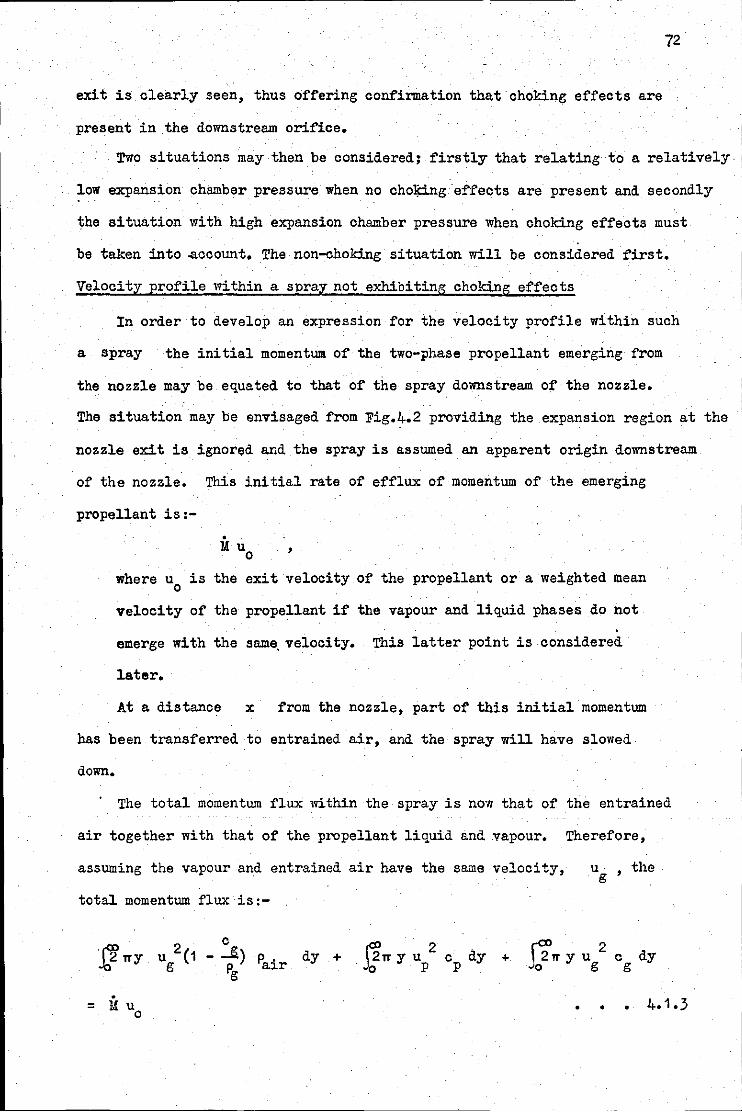
exit is clearly seen, thus offering confirmation that choking effects are
present in the downstream orifice.
72
I
' I
Two situations may then be considered; firstly that relating to a relatively 1
low expansion chamber press~e when no cho~g~effects are present and secondly
the situation with high expansion chamber pressure when choking effects must
be taken into ~ccount. The non-choking situation will be considered first.
Velocity profile within a spray not exhibiting choking effects
In order to develop an expression for the velocity profile within such
a spray the initial momentum of the two-phase propellant emerging from
the nozzle may be equated to that of the spray downstream of the nozzle.
The situation may be envisaged from Fig.4.2 providing the expansion region at the
nozzle exit is ignored and the spray is assumed an apparent origin downstream
of the nozzle. This initial rate of efflux of momentum of the emerging
propellant is:-
Yu0
,
where u0
is the exit velocity of the propellant or a weighted mean
velocity of the propellant if the vapour and liquid phases do not
emerge with the sam~ velocity. This latter point is considered
later.
At a distance x from the nozzle, part of this initial momentum
has been transferred to entrained air, and the spray will have slowed
down.
The total momentum flux within the spray is now that of the entrained
air together with that of the propellant liquid and .vapour. Therefore,
assuming the vapour and entrained air have the same velocity, u , the g
total momentum flux is:-
·~rry 2 c
u (1 - ~) g Pg
f(X) 2 2n y u
~0 g
• •
c dy g
•
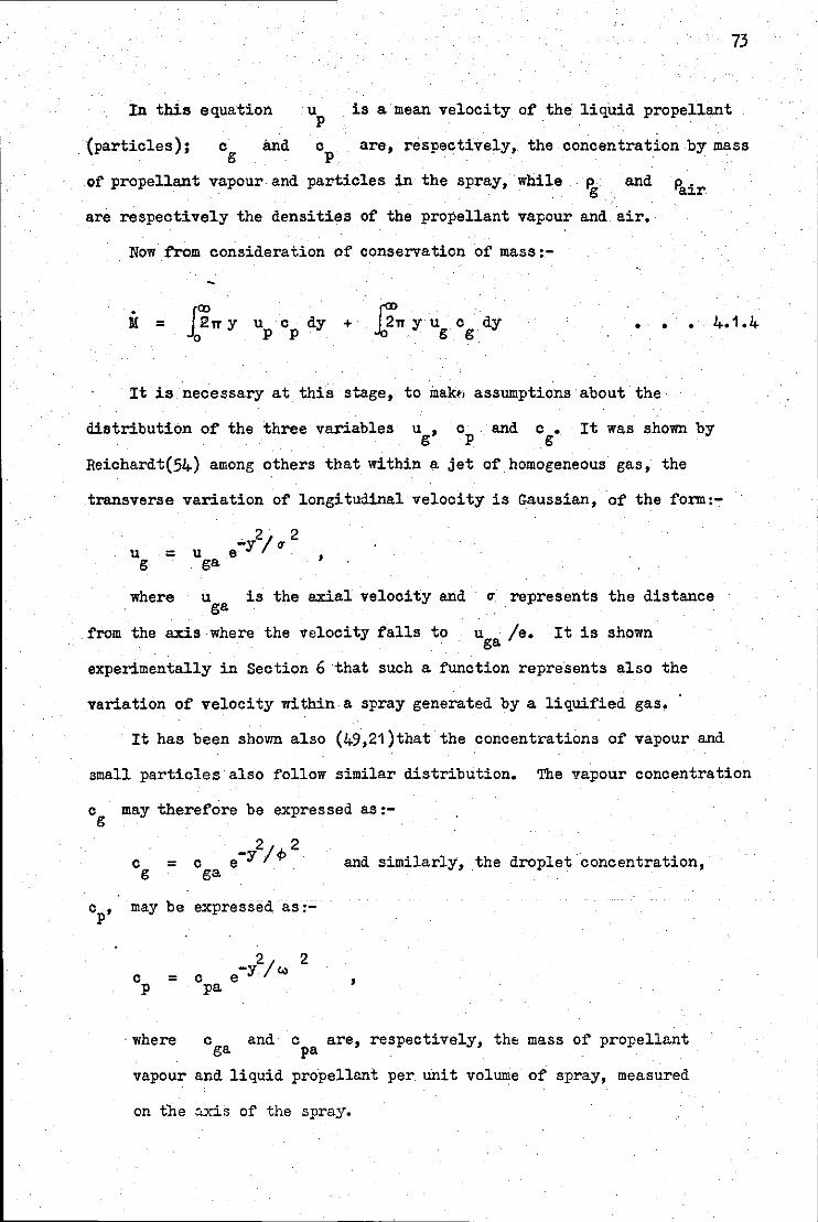
73
In this equation is a mean velocity of the liquid propellant
. (particles}; 0 g
and are, respectively, the concentration by mass
of propellant vapour and particles in the spray, while and
are respectively the densities of the propellant vapour and air.
Now from consideration of conservation of mass:-
. M = u c dy +
p p c dy
g •
It is necessary at this stage, to inak•• assumptions about the
• •
distribution of the three variables ug, op
Reiohardt(54) among others that within a jet
and c • It was shown by g
of homogeneous gas, the
transverse variation of longitudinal velocity is Gaussian, of the form:-
u g
= u ga e 2 2
•y /u '
where u is the axial velocity and u represents the distance ga
from the axis where the velocity falls to uga /e. It is shown
experimentally in Section 6 that such a function represents also the
variation of velocity within a spray generated by a liquified gas,
It has been shown also (49,21}that the concentrations of vapour and
small particles also follow similar distribution. The vapour concentration
cg may therefore be expressed as:-
0 g = c ga e -i/-t>2 and similarly, .the droplet concentration,
c may be expressed as:-p'
c p =
·where
c pa e 2 2
-y /c.o '
c and c are, respectively, the mass of propellant ga pa
vapour and liquid propellant per unit volume of spray, measured
on the ::..xis of the spray.
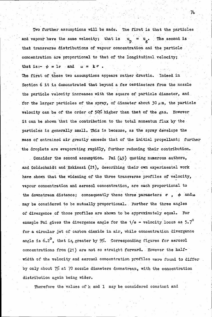
74
Two further assumptions will be made. The first is that the particles
and vapour have the same velocity; that is = u • g
The second is
that transverse distributions of vapour concentration and the particle
concentration are proportional to that of the longitudinal velocity;
that is:- </> = lcr al'ld "' = k u ,
The first of these two assumptions appears rather drastic, Indeed in
Section 6 it is demonstrated that beyond a few centimeters from the nozzle
the particle velocity increases with the square of particle diameter, and
:for- the larger particles of the spray, of O.iameter about 30 J.l m, the particle
velocity can be of the order of 50% higher than that of the gas, However
it can be sho;vn ·that the contribution to the total momentum flux by the
particles is generally small, This is because, as the spray develops the
mass of entrained air greatly exceeds that of the initial propellant; further
the droplets are evaporating rapidly, further reducing their contribution.
Consider the second assumption. Pai (49) quoting numerous authors>
and Goldschmidt and Eskinazi (21), describing their own experimental work
have shown that the_ widening of the three transverse profiles of velocity,
vapour concentration and aerosol concentration, are each proportional to
the downstream distance; consequently these three parameters u , </> andw
may be considered to be mutually proportional. FUrther the three angles
of divergence of those profiles are shown to be approximately equal. For . 0
example Pai gives the divergence angle for the 1/e- velocity locus as 5.7
for a circular jet of carbon <l.ioxide in air, while concentration O.ivergence
angle is 6.2°, that i~ greater by 9%. Corresponding figures for aerosol
concentrations from (21) are not so straight forward. However the half
width of the velocity and aerosol concentration profiles were found to differ
by only about 7% at 70 nozzle diameters downstream, with the concentration
distribution again being wider.
Therefore the values of k and 1 may be considered constant and
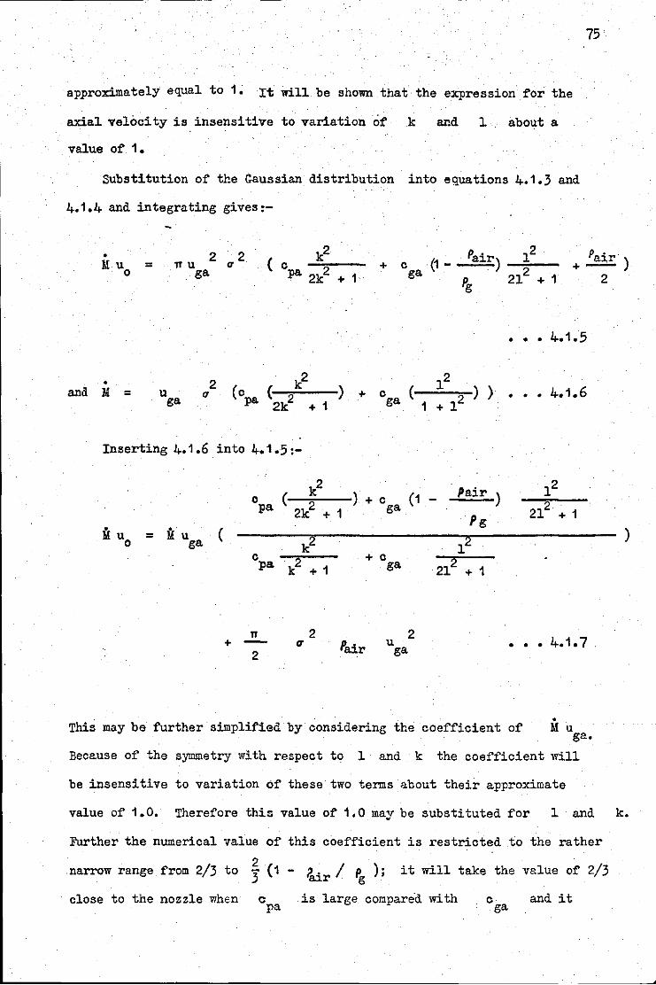
approximately equal to 1; It will be shown that the expression for the
axial velocity is insensitive to variation of k and l about a
value of 1.
Substitution of the ~aussian distribution into equations 4.1.3 and
4.1.4 and integrating gives:-
75
= 2
TTU ga
u 2 + c (1-ga
Pair ) +-
• 2 and Jd = u u ga
Inserting 4.1.6
• !.! u0
= Muga
(cpa k2
( 2k
2 + 1
into 4.1.5:-
(
c pa
cpa
n +-
2
( k2
2k2
+
k
k2
+ 1
2 tT
+ 1
) + c
) + c 1
+ c
Pair
ga
ga
ga
u ga
( 1
(1 -
2
• • • 4.1.·5
12 ) )
+ 12 ..... 4.1.6
Pair ) 12
212
+ 1 Pg
l
212
+ 1
••• 4-.1. 7
This may be further simplified by considering the coefficient of ir u ga.
Because of the s~~etry with respect to 1 and k the coefficient will
be insensitive to variation of these two terms about their approximate
2
)
value of 1.0. Therefore this value of 1,0 may be substituted for l and k,
Further the numerical -value of this coefficient is restricted to the rather
2 narrow range from 2/3 to 3 ( 1 - ?air / pg ) ; it will take the value of 2/3
close to the nozzle when c pa is large compared with and it
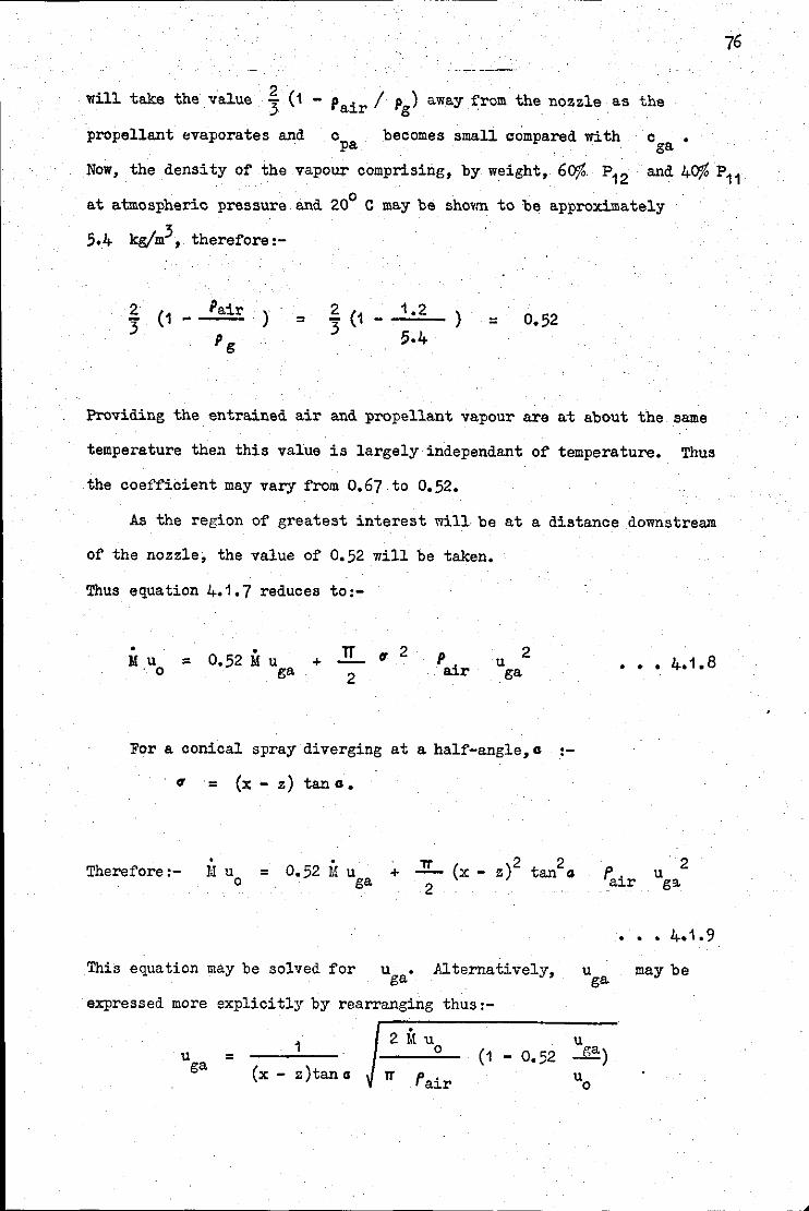
76
2 . wil~ take the va~ue 3 (1 - Pair/ Pg) away from the nozzle as the
propellant evaporates and opa becomes small compared with oga •
Now, the density of the vapo~ comprising, by w~ight, 60%. P12 and 40% P11 at atmospheric press~e and. 20° C may be shovm to be approximately
5,4 kg/m3, therefore:-
2 3 (1 -
Pair } = 2 - (1 -3
) =
Providing the entrained air and propellant vapour are at about the same
temperature then this value is largely independant of temperature. Thus
the coefficient may vary from 0.67 to 0,52.
As the region of greatest interest will be at a distance downstream
of the nozzle, the value of 0.52 will be taken.
Thus equation 4,1,7 reduces to:-
• Mu
·o = 0.52 i! u ga p air
2 u ga
For a conical spray diverging at a half-angle,o :-
t1 = (x - z) tan o ,
Therefore:-. Mu
0
• • • 4.1. 8
u ga 2
• • • 4.1. 9
This equation may be solved for uga' Alternatively,
expressed more explicitly by rearranging thus:-
u may be ga
u = ga 1
(x - z)tan Cl
r-~------------
2 t! uo u (1 - 0.52 ~)
1T fair
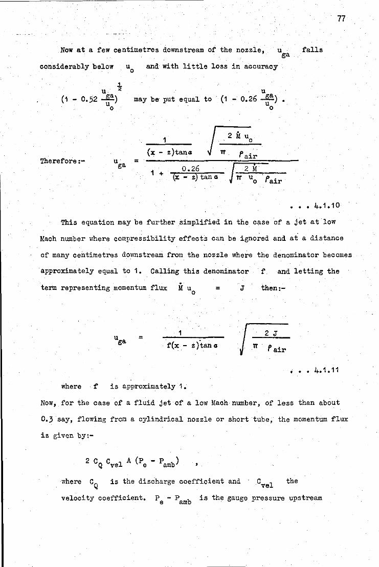
Now at a few centimetres downstream of the nozzle, u falls ga
considerably below u0
and with little loss in accuracy
~ u 2 u
(1 - 0.52 ~) uo
may be put equal to (1 - 0.26 ~) • uo
Therefore:- u = ga
1
(x - z )tan a
0.26
·~
J~ Tt fair
1 + (x - z) tan a ~ Jrru;;fair
77
••• 4.1.10
This equation may be further simplified in the case of a jet at low
Mach number where compressibility effects can be ignored and at a distance
of many centimetres dovmstream from the nozzle where the denominator becomes
approximately equal to 1, Calling this denominator f. and letting the .
term representing momentum flux M u0
= J then:-
1 =
f(x - z )tan a
• • • 4.1. 11
where f is approximately 1,
Now, for the case of a fluid jet of a low Mach number, of less than about
0.3 say, flowing from a cylindrical nozzle or short tube, the momentum flux
is given by:-
'
where is the discharge coefficient and the
velocity coefficient. Pe- Pamb is the gauge pressure upstream
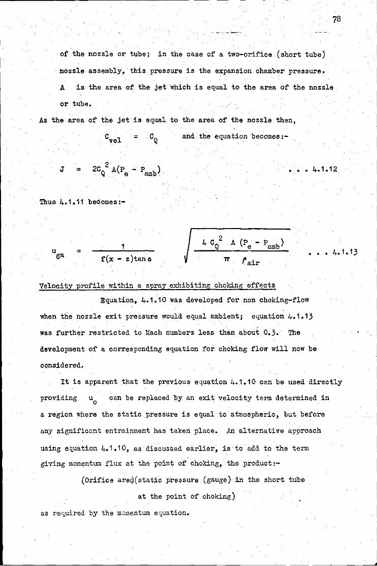
78
of the nozzle or tube; in the case of a two-orifice (short tube)
nozzle assembly, this pressure is the expansion chamber pressure.
A is the area of the jet which is equal to the area of the nozzle
or tube.
As the area of the jet is equal to the area of the nozzle then,
= and the equation becomes:-
J = 2 .
2CQ A(P - P b) e am . • . • • 4.1.12
Thus 4.1.11 beo.omes :-
u = ga 1
••• 4.1.13 f(x - z)tana fair
Velocity profile within a spray exhibiting choking effects
Equation, 4.1.10 was developed for non choking-flow
when the nozzle exit pressure would equal ambient; equation 4.1.13
was further restricted to Mach numbers less than about 0.3. The
development of a corresponding. equation for choking flow will now be
considered.
It is apparent that the previous equation 4.1.10 can be used directly
providing u 0
can be replaced by an exit velocity term determined in
a region where the static pressure is equal to atmospheric, but before
any significant entrainment has taken place. An alternative approach
using equation 4.1.1 o, as discussed earlier, is· to· add to the term
giving momentum flux at the point of choking, the product:-
(Orifice are9(static pressure (gauge) in the short tube
at the point of choking)
as required by the momentum equation.
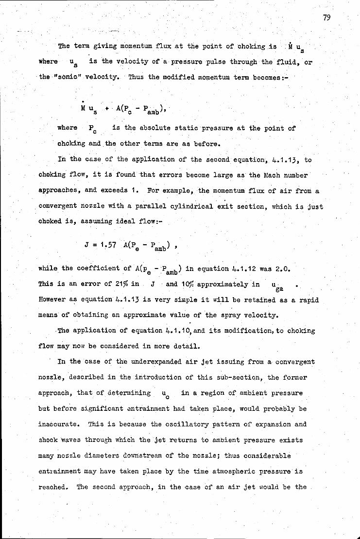
The term giving momentum flux at the point of' choking is .M us
where is the velocity of' a pressure pulse through the fluid, or
the "sonic" velocity. Thus the modified momentum term becomes:-
• M us + A(Pc- pamb)'.
where Pc is the absolute static pressure at the point of'
choking and the other terms are as before.
In the case of' the application of' the second equation, 4.1.13, to
choking flow, it is found that errors become large as the Mach number
approaches, and exceeds 1. For example, the momentum flux of air from a
convergent nozzle with a parallel cylindrical exit section, which is just
choked is, assuming ideal flow:-
while the coefficient of A(pe -·pamb) in equation 4.1.12 was 2.0.
This is an error of 21% in J and 10% approximately in u ga •
However as equation 4.1. 13 is very simple it will be retained as a rapid
means of obtaining an approximate value of the spray velocity •
. The application of' equation 4.1.1 o, and i.ts modification, to choking
flow may now be considered in more detail.
In the case of the underexpanded air jet issuing from a convergent
nozzle, described in the introduction of this sub-section, the former
approach, that of determining u 0
in a region of ambient pressure
but before significant entrainment had taken place, would probably be
inaccurate. This is because the oscillatory pattern o~ expansion and
shock waves through which the jet returns to ambient pressure exists
many nozzle diameters downstream of the nozzle; thus considerable
entrainment may have taken place by the time atmospheric pressure is
reached. The second approach, in the case of an air jet would be the
79
80
more suitable because the conditions within the nozzle of sucha system
are well established, The same is not true for two'-phase flow however.
In this case the behaviour of the two-phase propellant in the downstream
orifice and just beyond the orifice exit is by no means completely
predictable. However, from the two-phase flow literature a number of
relevant conclusions. can be made with considerable confidence. These are
now considered. Firstly there is general agreement that the static pressure
at the exit plane of a short tube is greater than ambient during mass
limiting flow, and that this pressure falls to ambient at a few nozzle
diameters from the exit plane. Secondly for fairly high quality flow,
for example greater than about 20% steam in steam/water flow (33), this
fall to ambient is accomplished by an initial excursion below ambient,a
phenomenon similar to that of an air jet; for low quality flow, however
this effect is absent. Thirdly shock waves may be observed in high quality
flow but are not present .in low quality flow. This is attributed to the
high momentum relaxation time of the liquid phase.
The application of equation 4.1.10 to the treatment of choking
two-phase flow will be considered inthe light of these three conclusions.
From the point of view of producing a fundamental expression the modified
equation, given again below, is the more satisfactory in that all the
terms in the result~~t expression are, in pri~ciple, predictable.
The expression is then:-
1 (x - z)tanc
2(M us+ A(Pc - pamb))
lr fair
••• 4.1.14
However as will be seen in the second part of this section, many assumptions
are required to produce expressions for the sonic velocity and the critical
81
pressure. Consequently the former method would enable a more direct
comparison between theory and practice. This method is considered applicable
because in this case of.low quality two-phase flow it is expected that there
will be no oscillator pressure wave pattern; instead the pressure is expected
to fall rapidly to ambient within a few nozzle diameters. Thus an exit'
-velocity in a region of ambient pressure would be measurable before significant
entrainment had taken place. Thus both methods will be considered, but
for the purposes of direct comparison between theory and experimental results, .
equation 4.1.10 will be used where M is the mass flow-rate and
is the velocity of spray a few nozzle diameters downstream of the nozzle.
This velocity will be denoted by u • . . n
A further point may be mentioned. This is that the liquid and gas
phases will be assumed to pass through the orifice with equal velocity.
This assumption is not in accord with the findings of Fauske ( 15 ) who
determined gas/liquid velocity ratios for pipe flow from direct measurement
of void fraction. It is however, substantiated by data presented in
Section 6. The Fauske findings would predict a gas/liquid velocity. ratio
of about 1.2. This is considered further in the next part of this section.
In order to reduce to a certain extent, the number of empirical
factors in this analysis, the possibility of equating the divergence
angle of the spray, which has been shown to consist mainly of air,to
that of an air jet will be considered. Limited experimental support
will be given in Section 6.
L----------------------------------------------------- --- -------~
I
82
4,2 Flow of a saturated liquid through a two-orifice nozzle assembly
In the previous sub~section, the axial velocity profile of a spray
was described by equation 4.1 .1 0 in terms of the mass flow-rate of
propellant and a discharge velocity determined at a point where the static
pressure within the spray was equal to ambient, In the case of a non-
choking flow this discharge velocity was simply the nozzle exit velocity.
For choking fl"Ow, equation 4,1,10 is still applicable providing an initial
velocity, u , exists and can be predicted, such that static pressure has n
fallen to ambient before significant atmospheric entrainment has taken
place, In the case of choking flow, however, the alternative equation,
4,1,14 may be used, From this ~t is seen that in order to describe the
axial velocity px·ofile theoretically it is necessary to predict, in addition
to the mass flow-rate, the critical or choking velocity and the critical
pressure. It is the purpose of this sub-section to predict these three
parameters for a two orifice nozzle assembly. The method adopted is outlined
below. Firstly an expression for mass flow-rate through this upstream orifice
is determined in terms of non-fundamental parameters. Secondly an expression
for the mass flow-rate through the downstream orifice is determined also
in non-fundamental terms, On equating these two expressions for the mass
flow-rates, an equation for the mass fraction of propellant evaporated is
obtained in tenns of fundamental parameters of the system. From this .
expression, the mass flow-rate through the nozzle assembly can be determined,
also in terms of fundamental parameters of the system. In the course of thene
derivations, fundamental equations for the critical velocity and pressure
are generated,
4.2.1 l.iass flow-rate through the uDstream orifice ~
The propellant entering the upstream orifice (short tube) is in
liquid form, The question then arises as to whether the propellant remains
in liquid form during its passage through this orifice, or .whether it will
evaporate as a result of the decrease of the pressure. A criterion by means
of which this question may be answered was developed by Pasqua ( 50 ). This
was described in the literature survey and is discussed more fully in
Section 6 where it is demonstrated that the propellant will indeed remain
as a liquid during its passage through the first orifice. The Bernoulli
equation may then be applied to this flow. This is given in BS 1042 as:-
4 D 4 1 - ( D1)
e
In this equation f 1 is the density of the liquid propellan~,
Pi is the absolute pressure upstream of the orifice and Pe is the
absolute pressure in the expansion chamber. is the discharge
coefficient of the orifice. D1/De· is the ratio of orifice diameter. to
supply tube diameter. The largest orifice used was 0. 7 mm anO. the tube
diameter was 3;2 mm, therefore, to within 0.2%· 1 - (D1/D )4 may be ' . e
considered equal to 1.
Therefore:-
• • • 4. 2.1
4.2.2 Mass flow-rate thropgh the downstream orifice.
(a) with a low pressure differential across the orifice.
The flow of a dispersed two-phase fluid through an· orifice is shown
83
in Fig. 4.3. The propellant passes through the do•mstream orifice in the
form of a liquid-vapour mixture. Unlike the previous case no single,
relatively simple, well proven theory exists which describes the passage
of a two phase fluid through a nozzle.
In order to obtain an equation for the mass flow-rate in a workable
Fig. 4.3
c
orifice
(short tube}
. c .,...1==1 :::> ----~-' <:::::: => < > C)
)
I I U ~ ~·U+dU
' l<:::k ==::;,-, <::::::::. c > I I
1 c:::c:::::::::_::::::=:>::::o c:::c::::::::::.-:. <::::::::::> I .
X-Secticnal area = A
Mean fluid density = p
FLO'!l OF A NO-PHASE FLUID THROUGH A SHORT TUBE
85
form, a number of assumptions must be made. They are discussed below,
(a} · The flow through the orifice is considered to be one dimensional
and also isentropic, that is adiabatic and frictionless.
Entrance and viscous losses that arise in practice are taken
into account by the introduction of a discharge coefficient cQ2
(b) The-propellant in the orifice is· assumed to be highly dispersed,
with.no large scale separation of the phases. Photographic
evidence presented in. Fig. 2.17 supports this view.
(c) There is no relative velocity between the liquid and gas phases.
This assumption was discussed in more detail in the previous sub-
section.In Section 6 experimental evidence is·presented in its favour.
(d) It is assumed that all the length of nozzle is short, typically
0.7mm, then there is no mass-transfer between phases during
the passage of the propellant through the orifice. ·This point
has been discussed in the literature survey. Fauske ('15 )
has shown that good agreement between theory and
experiment may be obtained, even with relatively long nozzles,
by maldng this assumption. It follows that the fraction of
propellant evaporated - sometimes called mass dryness fraction
or quality ·.(q), remains constant during the passage of the
propellant through the orifice.
(e) For the same reasons expressed in (d) above it is assumed
that there is no heat transfer between phases during transit
through the orifice.
(f) The propellant vapour is considered to be a perfect gas.
It follows from assumptions (d), (e) and (f) that during passage
through the orifice the propellant vapour obeys the isentropic gas

equation:-
L i' g
86
= constant
where y is .the ratio o:f specific heats at constant pressure and volume
:for the propellant vapour •.
Referring to Fig. 4.3 a differential element o:f :fluid is in the
process of passing through the orifice from the expansion chamber at an
absolute pressure o:f · Pe to the orifice exit where the· pressure is P0
•
Assuming no irreversibility then the exit velocity (u ) 0
is obtained
by integrating the one-dimensional Euler equation.
d p Therefore:- = . • . 4.2.2
2 r
where r is the mean density o:f the two-phase propellant.
Now:- 1 =
q + ..• 4.2.3
Pamb
2 1 - q
-I u q
Therefore:- 0 = (P .., p b) dP 2 rl e am rg
p e
• • •
It was shown above that during the passage through the orifice
and are related by the equation: p = constant, or
87
p
PY g
= where the subscript "e" refers to the expansion chamber.
.••• 4.2.5
pamb
1 y
Therefore:- = (1 .;. q) (P - p ) -amb q pe
. 1 dP
Therefore:-
2
2 u 0
2 =
The mass flow-rate is given by:-
=
e
fl
'IT
4
.p e.
1
pY
pY pge
. .• 4.2.6
- p b) + .q e 1 am f (1 - -)
1-1. ( p y
e ge Y
... 4.2. 7.·
• • • 4.2. 8
where is the density of the two-phase fluid at the orifice
·exit.
4.2.3 1\ass flow-rate through the downstream orifice.
(b) with a hir;h pressure differential across the orifice.
The derivation of the exr,ression for the exit velocity and mass flow-
rate of a two-phase fluid (equations 4.2. 7 and 4.2,8) did not include any
restriction on the magnitude of the ratio of the orifice exit pressure to
the expansion chamber pressure (P I p ) o e
or an upper limit to the value
1 1-p y)
- a.'llb
88
of the exit velocity u • · As discussed earlier, however, on lowering 0
the value of the pressure ratio across a nozzle discharging a compressible
fluid, the exit velocity u0
reaches a maximum, which is the velocity of'
a pressure pulse through the fluid. Ideally, further reduction of
downstream pressure therefore would not increase the velocity, or mass flow-
r~te through the nozzle. Under these conditions the flow is described
as critical, choked, or mass.-limiting.
A number of' authors have shown that choking flow occurs when liquid
and vapour mi~turea are discharged through nozzles, providing the ratio
of the downstream to upstream pressure is less than about 0.5, (for
example (63,12)).
It is considered that choking phenomena must.be taken into account
. when describing the flow through the downstream orifice (short tube).
This is because the pressure of' the propellant in the expansion chamber
during continuous flow discharge is typically 300 to 380 kN/m2 and the
absolute pressure ratio across the orifice is therefore 0.33 to 0.26.
These values are considerably lower than the generally accepted critical
pressure ratio of' about 0.5, indicating that choking flow conditions should
prevail within the downstream orifice. Although mass flow-rates at varying
ambient pressures were not made, it is considered that the existence of'
mass limiting flow was conf'iimed by the rapid expansion at the nozzle
exit of' the jet discussed in sub-section 4.1.
Referring to Fig.4.3, the pressure ratio PalPe is considered to be
small and consequently mass limiting flow conditions are considered to
prevail. The maximum velocity in the orifice is the velocity of' a
pressure pulse in the two-phase mixture (us).
An ex)lression for velocity us of a wave or pressure pulse
through a.~ isotropic homogeneous elastic medium is:- 1 2
u s
= df dP
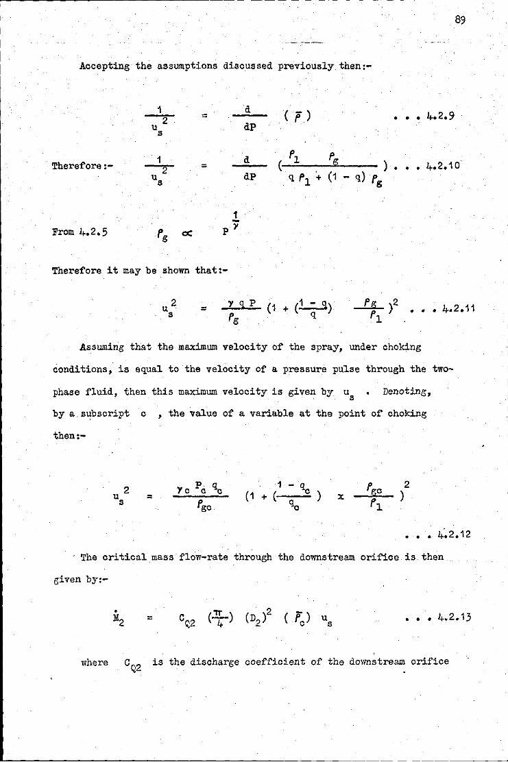
89
Accepting the assumptions discussed previously then:-
1 d ( f) •• 4.2.9 2 = • u dP s
f. 1 d ( fl
) Therefore:- 2 = • •• 4.2.10 us dP q fl + (1 - q) f g
1 -From 4.2.5 fg cc pY
Therefore it may be shown that:-
= 'Y q p
fg fg )2 • --'-~,.1- •• 4.2.11
Assuming that the maximum velocity of the spray, .under choking
conditions, is equal to the velocity of a pressure pulse through the two-
phase fluid, then this maximum velocity is given by u . a Denoting,
by a subscript c , the value of a variable at the point of choking
then:-
2 u s =
Ye p. q c c
fgc
1 - q (1 + ( ~ c ) :X:
2 )
• • • 4.2.12
· The critical mass flow-rate through the downstream orifice is. then .
given by:-
= ••• 4.2.13
where cQ2 is the discharge coefficient of the downstream orifice
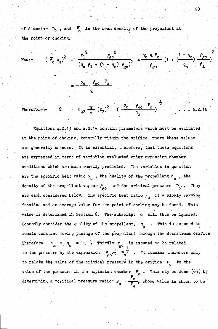
90
of diameter n2 , and ~ is the mean density of the propellant at
the point· of choking.
Now:- =
Ye =
•
f'gc
q
2 f'gc
p c·
t Ye f'gc Pc
Therefore·:- "IT (D )2 ( ) M = 0Q2 T 2 'le ••• 4.2.14
Equations 4.2.13 and 4.2.14 contain parameters which must be evaluated
at the point of choking, generally within. the orifice, where these values
are generally Unknown. It is essential, therefore, that these equations
are expressed in terms of variables evaluated under expansion chamber
conditions which are more readily predicted. The variables in question
are the specific heat ratio y , the quality of the propellant q , the c . c
density of the propellant vapour f and the critical pressure P . • They p c
are each considered below. The specific heat ratio y is a slowly varying c
function and an average value for the point of choking may be found. This
value is determined in Section 6. The-subscript o will thus be ignored.
Secondly 90nsider the quality of the propellant, q0
This is assumed to
remain constant during passage of the propellant through the downstream orifice.
Therefore = q . e = q • Thirdly o is assumed to be related . 'gc . 1
to. the pressure by the expression ~"gc a:: p o "f It remains therefore only
to relate the value of the critical pressure in the orifice Pc to the
value of the pressure in the expansion chambe.r P • . p e
This may be done (63) by
detennining a "critical pressure ratio" r0
= T• whose value is e
shown to be
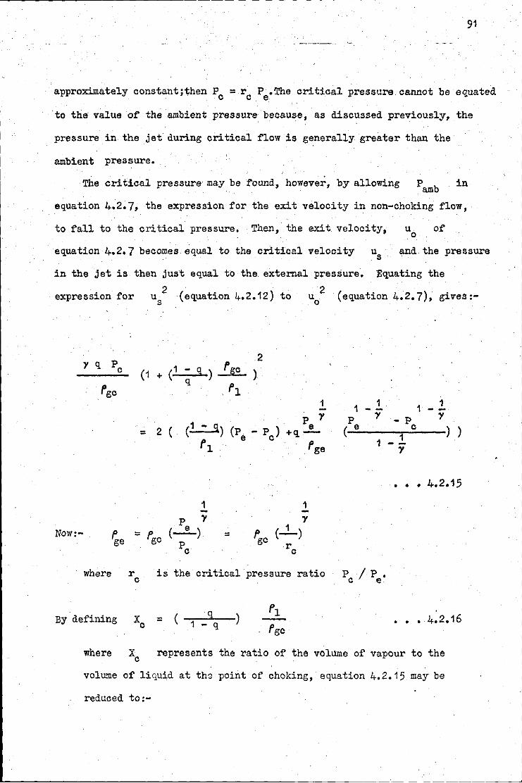
91
approximately constant;then P = r P .The critical pressure cannot be equated c c e
to the value of the ambient pressure because, as discussed previously, the
pressure in the jet during critical flow is generally greater than the
ambient pressure.
The critical pressure may be found, however, by allowing P amb in
equation 4.2.7, the expression for the exit velocity in non-choking flow,.
to fall to the critical pressure. Then, the exit velocity, uo of
equation 4.2.7 becomes equal to the critical velocity us and the pressure
in the jet is then just equal to the. external pressure, Equating the
expression for (equation 4.2.12) to u 2 ·(equation 4.2.7), gives:o
pc 2
y q (1 + (1 - 9. .!.ra ) )
f'gc q ,.1
1 1 1 1 1
Pe y p y
- p y
2 ( (1 - q) (P - p ) ( e c ) ) = +q- 1 f' e c f'ge 1 1 y
••• 4.2.15
1 1
p y y
Now:- ~e = f'gc (_!.._) = ,Pgc (....L)
pc re
where r is the critical pressure ratio Pc/ pe' c
By defining = ( -1,...-;-'"""q-) • • • 4.2.16
where Xc represents the ratio of the volume of vapour to the
volume of liquid at tho point of choking, equation 4,2,15 may be
reduced to:-
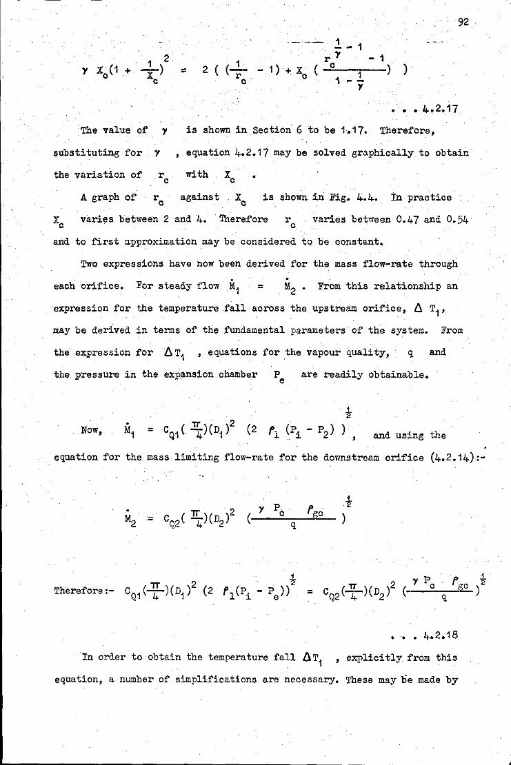
92
---·- 1 1 --...1...)
2 ( (...1...
r'Y - 1 ., Xc(1 2 - 1) + Xc ( c ) ) + ::: 1 XC re. 1 --y
The value of y is shown in Section· 6 to be 1.17. Therefore,
substituting for Y , equation 4,2,17 may be solved graphically to obtain
the variation of r0
with Xc •
A graph of r0
against X0
is shown in Fig. 4.4. In practice
x0
varies between 2 and 4. 'Therefore r varies between 0.47 and 0.54 c
and to first approximation may be considered to be constant,
Two expressions have now been derived for the mass flow-rate through .
each orifice. For steady flow M1 = M2 • From this relationship an
expression for the temperature fall across the upstream orifice, ~ T1 ,
may be derived in terms of the fundamental parameters of the system. From
the expression for ~T1 , equations for the vapour quality, q and
the pressure in the expansion chamber Pe are readily obtainable.
Now, ~
M1 = CQ1 ( ~)(D1 )2 (2 fl (Pi - P2) ) , and using the
equation for the mass .limiting flow-rate for the downstream orifice (4,2.14) :-
i ·2
)
••• 4.2,18
In order to obtain the temperature fall ~T1 , explicitly from this
equation, a number of simplifications are necessary, These may l:ie made by
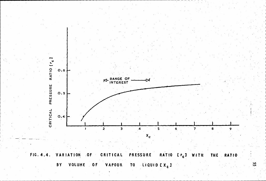
~--------------------------------------------------------------------------~---------------.
-u ... -0 0.6 ,._ < a: RANGE OF
r<3- INTEREST I>(
1.1.1 a: ::> lJ) 0. 5 lJ)
w a: (l.
...1 < u 0.4 ,._ a: u
2 3 4 s 6 7 8 9
Xc
-FIG. 4.4. VARIATION OF CRITICAL PRESSURE RATIO t rcl WITH THE RATIO
BY VOLUME OF VAPOUR TO L IQ U I 0 C X cl
94
considering in more detail the behaviour of the propellant
in the process of discharging through the nozzle assembly. Firstly
consider a relationship between the density of the propellant vapour, fge ,
in the expansion chamber and the expansion chamber pressure, Pe • It is
shown in Section 6 that for a nozzle assembly whose orifices are of
approximately the same diameter, the temperature fall across the first
orifice is less than about 6 deg c. Thus to a first approximation the
temperature in the expansion chamber may be considered to be constant
providing the diameter of the second orifice is not more than about t>tice
that of the first. Therefore the density of the propellant vapour in
the expansion chamber may be taken to be proportional to the pressure
within the expansion chamber {P ). e
Therefore:- fge == c1 pe
where c1 is determined tor Q temperature of about 16° c. 1
PO y Now, from before, fgc ::: l'ge (-)
Pe
and. also:- Pc ::: r Pe 0
where r is approximately constant. c 1 -p y
Therefore fgo ::: c1 p (~ ~) e c p e
1
or f'go = c1 pe re y
• • • 4. 2.19
• • • 4.2.20
The above restriction on the ratio of orifice diameters or temperature
variation, does not detract from the ·va.lue of this theory because, in
commercial practice, the diameters are usually approximately equal.
Maintaining this restriction on temperature variation, a further
95
• simpli~ication may be made. This is that mass ~raction of propellant
evaporated q , is proportional to the temperature fall across the first
, Therefore:-
0 • 0 4.2.21
In this equation c2 is determined over the range. 14°C to 20°c.
A third simplification will now be made. This is to express the pressure
fall across the first orifice !!!. P1 in terms of the temperature ~all !!!. T1 ,
again assuming a restricted range o~ expansion chamber temperature. If
conditions of thermodynamic equilibrium exist in the expansion chamber then
Pe = SVPTe , .Also i~ the propellant above the ~irst orifice is saturated
then Pi = SVP Ti • Therefore:-
For a small change in temperature the chanee in SVP is proportional to that
temperature change. Therefore:-
•.. 4.2.22
This applies for equilibrium above and below the first orifice. If the
propellant above the first orifice is sub-cooled by a head of propellant
above the nozzle, as is usually the case, then :-
+ 6P 0 0 0 ex
where I!!.P9x is the pressure due to this head,
The simplified expression for fgc , q and Pi - Pe may now
be substituted into equation 4.2,18. Therefore:-
L---------------------~----- - - - - -
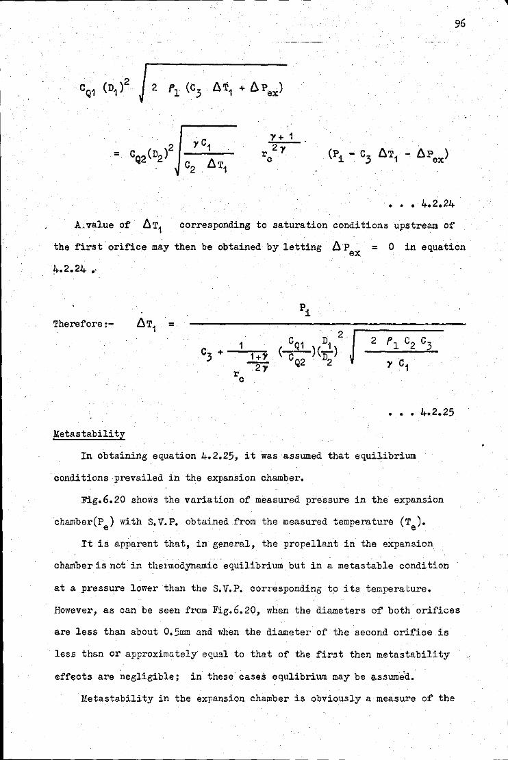
A,value of 6T1
Y+ 1 2y
re
••• 4.2.24
corresponding to saturation conditions upstream of
96
the first orifice may then be obtained by letting 6 P = 0 in equation e:x:
~..2.24 •.
pi Therefore:- 6T1 =
2
J 1 CQ1 D 2 l'1 c2 °3
c3 + 1+Y (
CQ2 )(...1)
~ . D2
Y c1 re
••• 4.2.25
Metastability
In obtaining equation 4.2.25, it was assumed that equilibrium
conditions prevailed in the expansion chamber.
Fig.6.20 shows the variation of measured pressure in the expansion
chamber(P ) with s. V.P. obtained from the measured temperature (T ), e e
It is apparent that, in general, the propellant in the expansion
chamber is not in thermodynamic equilibrium but in a metastable condition
at a pressure lower than the S. V.P. corresponding t.o :its ter.~perature.
However, as can be seen from Fig.6.20, when the diameters of both orifices
are less than about 0, 5mm and when the diameter of the second orifice is
less than or approximately equal to that of the first then metastability
effects are negligible; in these cases equl:ibr:ium may be assumed.
Metastability in the expansion chamber is obviously a measure of the
L------------------------------------------------ -- -- -
97
difference betwaen the rate of escape of vapour through the second orifice
and the rate of production of vapour by propellant in the expansion chamber.
Now, the rate of escape of vapour through the second orifice is
relatively high if the quality of the vapour q is high. Further the
rate of production of vapour will be low if the residence time of the
propellant in the expansion chamber is short. Therefore an elementary
model of metastabili ty would indicate that metastability effects might be
proportional to q and inversely proportional to some power of the
residence time in the expansion chamber, the latter given by:-
.J;.-- x (expansion chamber volume). M
It will be shown in Section 6 that generally terms such as quality •
q and mass flow-rate M can be expressed very simply in terms of the
orifice diameters. Thus q is found to be proportional to (D2 / n1 )2
and M to (D1D2 ). It may be expected therefore that metastability
defined as :-
llP = meta
may be similarly expressed.
An empirical correlation between llP t and me a .
from the data shown in Fig.6.20. The. relationship is:-
D4 "P = 1 ;80 x 103 (SVP at T ), X --=2~,..--L.l meta e D 2,5
1
where n1, n2
are in metre.
••• 4.2.26
... 4.2.27
This is plotted, together with the experimental data, in the Figure.
Metastabili ty may now be incorporated in the expression for ll T1 ·
Substituting
and
SVPTe - llPmeta
SVPTi + llPex
for Pe
equation 4.2. 23
98
··becomes:-
and therefore:-r------------------------------
r c
y + 1 2y
(Pi- C3 fjT.1 - fjp - fjp t ) ex · me a
Or, letting t:J. P ex become zero, as before,
1 y + 1
re 2 y
••• 4.2.28
••• 4.2,29
where Pi is now the S.V.P. of the propellant at T. J.. •
By substituting equation 4.2.27 into 4.2.29, l:J.T1 may be obtained
in tems of n1. , D2 , Pi and constants obtainable from thermodynamic
data, Rowever, equation 4.2.29 may be simplified by noting that for the
range of nozzles tested in these experiments
about a half of • Therefore:-
fj P t is always less than me a
(1 + ~
This is accurate to within at least 35~,11hile for nozzle assemblies with
n1 ~ n2 the ·error is considerably less.
Therefore:-
C D 2
12 c3 c2 6 Pmeta 1 (_9.1.)(....2.) rl (6T1
1 ) y + 1 +2
r 2y CQ2 D2 Y c1 c3 c
••• 4.2.30
Therefore:-Pi - 6p meta (1
1
••• 4.2.31
where Pi is now·ths s.v.P. at T1 and 6Pmeta may be obtained
from equation 4,2,27. It may be noted that Pi is much greater
than the term containing tl P • the latter is thus a small meta'
correction for the effect of metastability on the temperature fall,
The application of this equation to the determi.>ation of mass flow-
rate and expansion chamber pressure is demonstrated in Section 6.
99
)
5, EXPERIMENTAL
5.1 ExPerimental and au:rl.lary equipment
5,2 Calibration
5,3 Experimental programme
5,4 Experimental procedure
The purpose of the experimental progra.mn:e was two-fold; firstly,
to provide experimental evidence in support of the theoretical
expressions given in Section 4; secondly, to provide experimental
data relating to continuous sprays from which empirical expressions may
be developed.
The apparatus was designed to permit the study of a continuous
spray. This was generated by the flow, through a two-orifice nozzle,
of a saturated liquid at high pressure containing a surf'ace-active
5olute of low volatility,
Particle size and velocity distributions of droplets at selected
points within the spray could be measured together with other parameters
relevant to spray behaviour. These were: the pressure and temperature
of the propellant up-stream of , and inside, the nozzle assembly; the
rate of flow of propellant; and the size distribution of the residual
surf'actant aerosol.
5,1 Experimental Apparatus
The continuous flmv apparatus is· shown diagramatically in Fig. 5.1
and photographically in Fig. 5,3, Details are given in Figs 5,2 to 5,7
100
A brass bottle supplied saturated liquid propellant via a flexible feed
pipe to a nozzle assembly mou.'lted on a support capable· of movement in two
dimensions. The spray. emerging from the nozzle could be photographed
by a double-exposure photomicrographic unit. The spray could also be
collected in a sedimentation cylinder (not sho;m). Temperatures and
pressures at the various positions indicated could be measured.
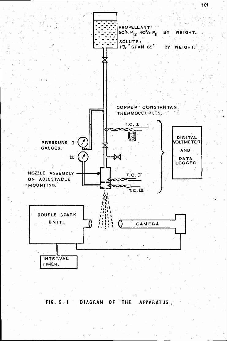
PRESSURE I GAUGES.
II
- - . -- . - .. - - - - -- - • • PROPELLANT' :-:-:-::60.,oP12 40%P11 BY WEIGHT. - - .
• • • • SOLUTE• - • .-·-·__. 1%" SPAN as'·' BY WEIGHT.
COPPER CONSTANTAN THERMOCOUPLES.
T.C. I
DIGITAL VOLTMETER
AND
DATA LOGGER.
NOZZLE ASSEMBLY --H---1>1 . T.C. n ON ADJUSTABLE
MOUNTING.
DOUBLE SPARK
UNIT.
INTERVAL TIMER..
FIG. 5.1
,; I I' . f J I '
' I t I ' I • 11 l I .,
•:···· I 1 I 1 ' I I I ' \ . .
T.c.m
CAMERA
DIAGRAM OF THE APPARATUS.
101
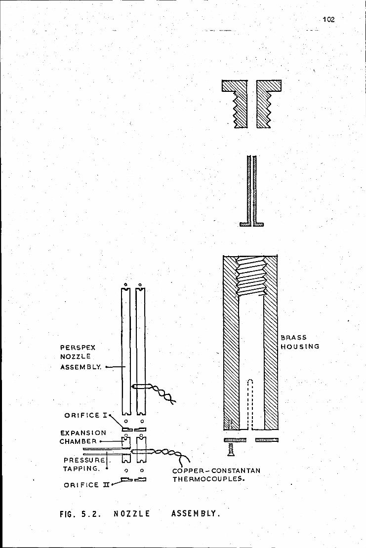
0 0
BRASS
PERSPEX HOUSING
NOZZLE
ASSEMBLY. --1-
ORIFICE I" -0
-
~o EXPANSION 0 "7 CHAMBER • Ll
PRESSURE!. W TAPPING. 0 o
ORIFICE II~c:::::l
FIG. 5.2. NOZZLE
'"i""''" 1!!1!1''"'''' !11
COPPER- CONSTANTAN THERMOCOUPLES.
ASSEMBLY.
102
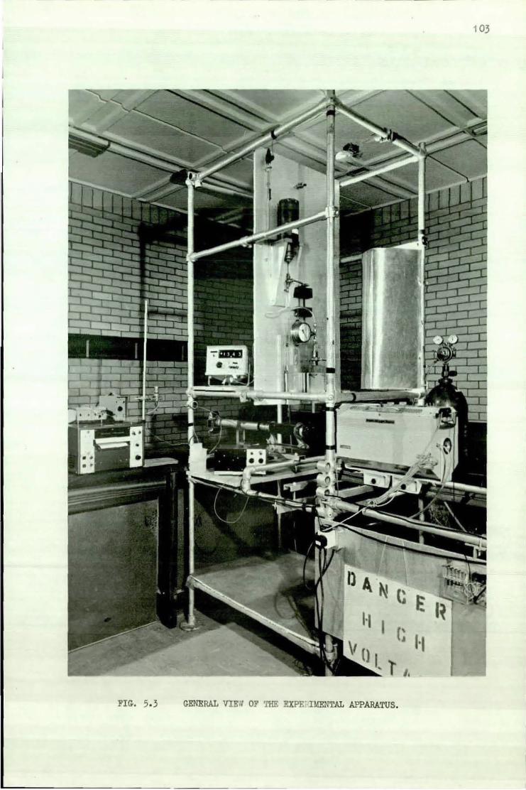
103
FIG. 5.3 GENERAL VlEil OF 'fHE EXPE ll!ENTAL APPARATUS.
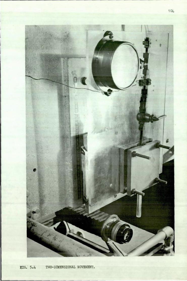
EIG. 5. 4 Two-DIMENSIONAL WOVEYENT.
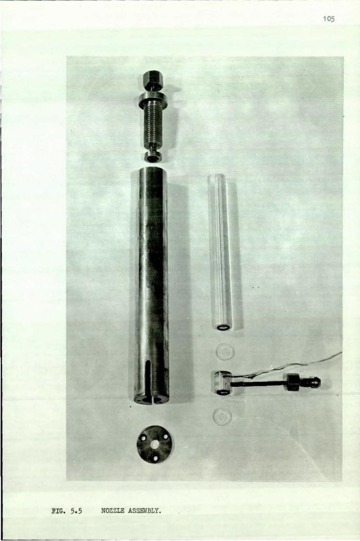
105
-
FIG. 5. 5 NOZZLE ASSEMBLY.
"------------- - - - - -
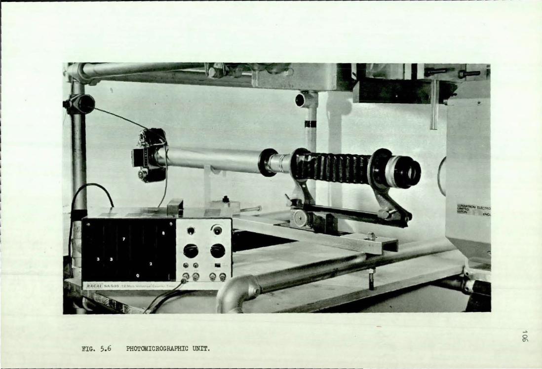
FIG. 5. 6 PHOTOMICROGRAPHIC UNIT.
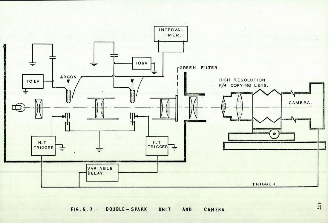
n --10 kV
ARGON y
I ~---~':i ··-~ ;.;·. t· 'i
H.T TRIGGER .
10 kV
INTERVAL TIMER .
" - rRLEEN FILTER HIGH RESOLUTION
L----~ ""! : F/4 COPYING
.--. fl ... - _------... -~·.· · .. ' t:~ . < ~ -
1...--..l
VARIABLE DELAY .
H. T TR.I GGE
TRIGGER .
FIG.5.7. · DOUBLE-SPARK UNIT AND CAMERA.
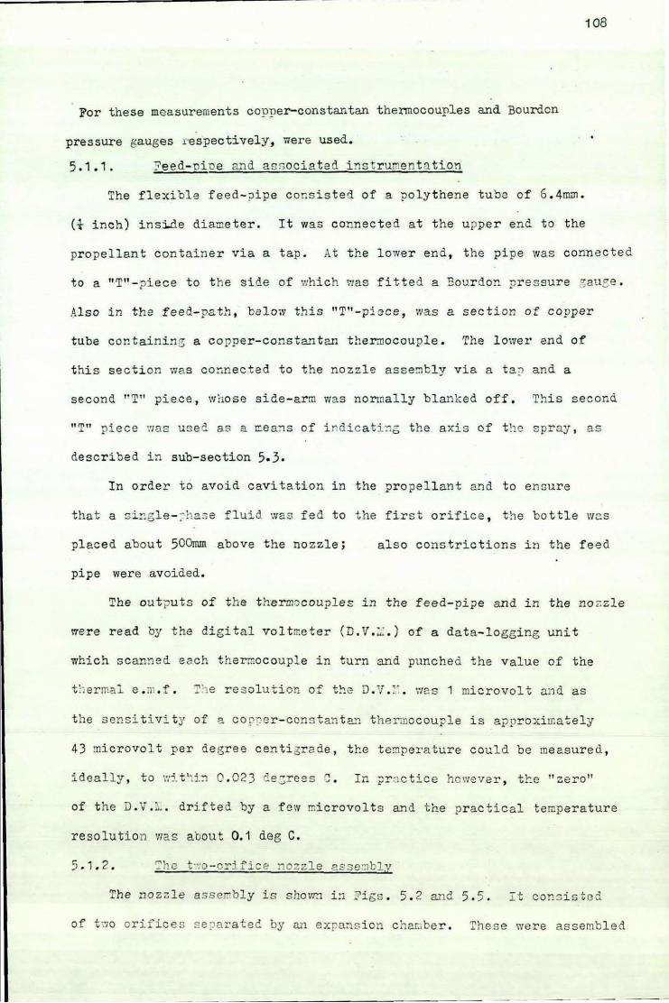
------------------------------------------------------- -
For these mea surements copper-cons t antan thermocouples and Bourdon
pressure gauges J.·e~pectively, i7ere used.
5 .1 . 1. 7e ed- oine and associ a t ed i ns t rument a tion
The fl e:cible fe ed- pi pe cons i s ted of a poly t hene t ube of 6 . 4mm .
108
(t i nch) i nsi.de diameter . It was connec t ed at the upper end t o the
pr o pellan t con taine r vi a a t ap . At t he lower end, t he pipe was conn ected
to a "T'' - ?iece to t he s i de of which was fi t t ed a Bour don pr es sure ~auee .
Al so i n t he feed- path , bel ow t his "T"-pi~ce, was a s ec t i on of c opper
t ube con tainine; a c opper - constan tan t her:nocouple . The l ower end of
t hi s section ~7as connected t o t he nozzl e as senbly via a ta~ and a
second " T" pi ece , whose s i de- arm was normally blanked off . Thi s s econd
"T'' piece '.'/as us eC. as a J!e a>1s of i ndi cati:1g the a xi s of t he spr ay , as
descr i bed i n sub- section 5.3.
I n order to avoi d cavi tati on in the pr ope l l ant and t o ensure
that a si~gle- ~hase fluid was f ed to t he first orifice , t he bottl e wc s
pl aced about 500mm above t he nozzle;
pipe were avoided.
als o constr i ctions i n the f eed
The outpu ts of the t hermocouples i n the f eed-pipe and i n the no r. zl e
\Ve re r ead by the di gi t al voltn:e te r (D . V . ~ . ) of a da t a- l oggi ng unit
which s canned ea ch t hermocouple i n turn and punched t he valu e of the
t ~1 ermal e . m. f . 1''1e r es ol uti on of the D. Y. :'' , was 1 microvolt <.:md as
t he s ens i t i vi t y of a co r?e r - ccnstan t a.Tl t he r mocouple is appr oxi mat el y
43 micr ovol t per degree cent i gr a de , t he t empera tur e coul d be measured ,
i deally, t o wi t '1i:1 0 . 02 3 1e3ree s ':: . In pr :.1c t ice however , t he "zer o"
of t he D. v .;, . dr ifted by a f~w mi crovolts and t he pr actical t emperature
re sol ution was about 0. 1 deg C.
5 .1. 2 . : he t ···o- c:df i ce nozzle esse:nbly
The nozz l e asse~bly i s sho~ i~ 7igs . 5 . 2 and 5. 5. It consi s t ed
of t \70 or ifice s s eJar a teC. by an expa.."ls i on char..be r . These wer e as sembl ed
~~~====~======~~~~~~~-------------------- -109
together. with a 150mm long perspex tube, ina brass cylinder. The nozzles.
which were made of perspex, were transparent and dismountable. This
arrangement had three adv~~tages. Firstly, it was possible to observe
the two-phase fluid flow in the expansion chamber. Secondly, it was
possible to apsure that bubbles, formed in the liquid approaching the
first orifice at the start of spraying, had discharged from the system
before measurements were talcen. Thirdly, different orifice combinations
could quickly be formed, and blockages eRsily removed,
· Two difficulties were associated with the use of perspex in contact
with the propellant. Firstly, according to the mw,ufacturer's
literature, perspex is sparingly soluble in halogenated hydrocarbons.
Secondly, perspex tends to "craze" along stress lines. To test the
effect of solubility, a nozzle was made up and the orifice .diameters
were measured with a microscope. Propellant was sprayed through the
nozzle for many hours durine; preliminary trials. Afterwards, the
diameters were again measured, l!o change in diameter was detected;
therefore the effect of solubility was ignored,
Crazing along stress lines was a more serious problem, After a
few minutes of spraying, cracks would appear in the ·perspex tube leading
to the nozzle and in the perspex of the expansion ch~mber; the orifice
sec tion.c, ~1owcver, were unaf:ectecl. These difficulties were overcome
by rumee.lin;; and coa tinr; with l.raldi te embedding resin as explained
below,
Nozzle Pmnufe.cture
The nozzles w,,re made as follows. A 150mm ( 6") perspex tube, of
12,7m 0-") outside diameter (O,D.) and J,2lllJ1'! (i.") inside diameter (I.D.)
was feced o~ 2. lathe, and an "0"-rir:.s .:;roove cut in one end. ..\ secozld
perspex tube 12. 7mm ( -}") long was machined sirr.ilarly with "0" -ring
grooves cut in both ends. Zach piece of perspex was annealed at 90°0

in an OV!'!n for about half a day. Two small holes were then dr'illed
through one side of the 12. 7m!n length of perspex. Through one hole,
110
a copper-constantan thermocouple was inserted and, after degreasing,
was sealed with resin •. The other hole was tapped with a 5 B.A. thread
and into it was screwed a hollow co;;per tube, similarly threaded;
this was also sealed with resin and thus served as a pressure tapping.·
This 12.7rrm leneth of perspex.became the expansion cha~ber in which
both temperature and pressure could be rn~asured. A thermocouple was
similarly inserted in the 150mmtube; within about 6mrn of one end.
Similar150mm and 12.7w.m perspex tubes, with no pressure tappings or
thermocouple tappings, were also made.
These pers!)ex tubes were then degreased and o. thin film of resin
. allowed to run down the centre of each and also over the machined .
faces. Excess resin was removed and the tubes were again placed in an
oven at S'0°C in order to hP.rden the resin and. further anneal the
perspex. This process prevented the crazing referred to above•
The orifice sections were then made from 1.6r.".m (1/16"). perspex
sheet, using a high-speed watchmaker's lathe as follows. A disc of
perspex 1.61l'm (1/16") thick and about 25mm in diameter, was cemented
by its outer edge to a perspex m~;dril inserted in the lathe chuck.
A drill of a;:;;;ro;:>rio.tc dimr.eter "!as held in a pin-chuck inserted in
the tail-stock of the lathe. The drill was used to cut a fine hole in
the perspex. ·The ce:1tre of the disc was then faced down until the
thickness of the perspex surroi..!!:din.,; tho hole '.7as approximately equal
to the diameter of the hole. The walls of the drilled hole (orifice)
were then polished by rotating the perspex disc about a thread of
cotton i~-F1·eg;:1atcC. with pc"!:'Si1ex polis!1. In order that the. orifice
walls should re~ain pnrRllel d.urin.~ !JOlishi!l:-:;, the thread '.·:as po.si tioncd.
alon:; the lat~1e axis. 'ihis was done by inserting one end of the thread
111
in the pin-chuck of the tail:..stock and the other end, over an aligned
"V" guide, to a weight. After about 5 minutes polishing, first with
coarse then with fine polish, the disc was removed from the mandril.
This v1as done by turning the disc down to 12. 7mm ( ~") diameter. Thus
an orifice section of the required diameter was obtained. The orifice
.was then inspected en a stereoscopic microscope and its diameter and
thickness measured· at a number of positions. Fifteen orifice sections,
whose dimensions are given in Appendix A1, were similarly manufactured.
Finally, the brass tube was manufactured, conventionally, on a
lathe, and the nozzles could then be assembled when required, as
indicated in Fig. 5.5.
During the early part of this project, the nozzles were stuck
together using resin as seen in Fig. 5.4, but this arrangement proved
rather unsatisfactory as a blockage of the inner orifice was difficult
to remove.
Two-d.il':'lennional nozzle move!!lent
The ·emerging spray was axially symmetrical. Therefore photographic
data, representative of the whole spray could be obtained by photography
along the spray axis and in one plane containing this axis. To do
this without disturbing the accurate alignment· of the optical system
it t:as necessn:r:r to r:ou:?.t. the nozzle such tr.n.t rr:ove:r.e:nt relative to
the camera was rossible. Therefore the nozzle v1aS clamped to a mounting
which permitted vertical and horizontal movement in the plane normal
to the axis of the optical system. ~his is shown in Fig.5.4. It consisted of
a 150n~ square x 12mm thick duralumin block which could be moved vertically, in
guides, by a. screw thread. icountecl on this block wa.s a smaller block,
also guided, which was ca."able of horizontnl rr.ove;wmt :Jo=al to tee
camera axis. The nozzle holder, which was mounted on this smaller block,
consis~ed of two 12mm thick rlates with a vertical eroove milled into
112
the inner surface of the outer plate, The nozzle was clamped in this ·
groove,
5.1.3. Double-exposure photomicrograohic unit
To obtain particle size and particle velocity measurements within
a spray, double-exposure and single-exposure photographs were taken
with a double-exposure photomicrographic unit, A specification for
such a system was obtained as follows. It was considered necessary
to obtain streak-free images of all particles resolved by the opticl':l
system, Also, for velocity measurements, it was considered essential
that the double images produced should be close enough together for
easy identification, but sufficiently far apart for accurate measurement
of their displacement.
Now the practical resolution limit of the photo-micrographic uriit;
as explained later, was. a few microns and maximum velocities within
the sprays were lmown, from preliminary experimentation, to be about
40 metres per second. Therefore the required period of exposure, l7hich is
given approximately by:-
diameter of smallest resolved ~erticle
particle velocity
was of the.order of 0,2 microseconds.
The minimum tirr.e intervPl between e:{posures was considered to be
that which ;ave an ime.3e dispbce:-cent of 10 times the diameter of the
smallest resolved particle. This min:l.mum interval was therefore in the
order of two mic1:'oseconds, al thou·g,~1 in practice 2.n i:1 terv2l of 10
microseconds proved to be more suitable.
To provide, conveniently, exposures of such duration, a ·double-
pulse spark u~1it v1as used. A suitable unit r;as ~anufactured by LWlartron
Electronics Limited. To the basic unit •.vere added, as explained belo•:1,
an interval timer and an F/1 condenoer lens, A photographic record was
113
obtained. with a camera systeo, shown, together with the spark unit in
Fig. 5. 7.
Double-snark u~it
The double-spark unit consisted of two spark gaps on the same
optical axis-with a system Of condenser lenses arranged so t~at each
:;,;:ark appeared to originate frorr. the same position. The spark duration
was about 0.2 microsecond.
The spark discharges were initiated by two H.T~ trigger units.
A delay unit was included which enabled the front spark to be triggered
a. pre-set interval of time after the rear spark. The magnitude of
this interval, which was set by a dial, was reproducible to.:!: 1%. The
minimum time interval between sparks on the standard spark unit was
20 microseconds. In order to obtain shorter intervals, a timing
capacitor was replaced in the delay unit. In this way, time intervals
down to .two microseconds were achieved,
It was necessary to calibrate the delay unit. This was done with
an oscilloscope as follows. Two insulated wires, placed close to each
spark gap, were fed to the "Y" input of the oscilloscope. · When the
spark unit was operated, each spark generated an induced e.m.f. in the
corresponding wire. The first spark trisgered the oscilloscope; thus
both pulses were conveniently displayed on the screen. Keasurement of
the distance, on a screen, between the two pulses enabled the time
interval between them to be determined with an accuracy of about 0.2
microseconds. The interval was then adjusted to the nominal value on
the dial of the delay unit.
',Yhen photographs were taken, this time interval was continuously
rronitored usin:; a !lr.cal interval tir::er which was started and stopped
by the inductive pick-up system previously described. The resolution
of the tir:1er was relatively long, however, (1 microsecond), a:1d it was
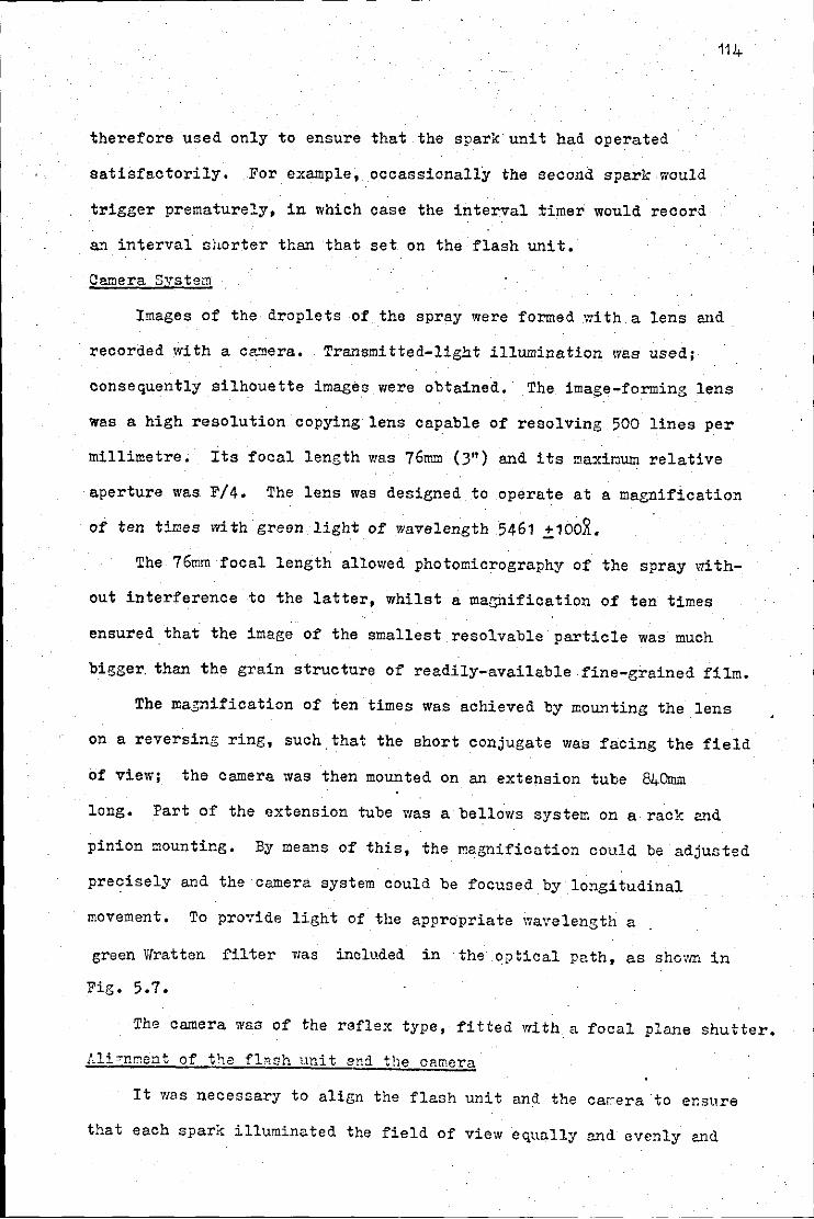
therefore used only to ensure that the spark unit had operated
satisfactorily, For example, occassionally the second spark would
trigger prematurely, in which case the interval :timer would record
a."l interval shorter than that set. on the flash unit.
Ca.-nera System
114
Images of the droplets of the spray were formed with a lens and
recorded with a ca.-nera. Transmitted-light illumination was used;
consequently silhouette images were obtained. The ima;;e-forming .lens
was a high resolution copying lens capable of resolving 500 lines per
millimetre. Its focal length was 76mm (3") and its maxinum relative
aperture was F/4. The lens was designed to operate at a magnification
of ten times with green light of wavelength 5461 ~100j,
The 76mm focal length allowed photomicrography of the spray with
out interference to the latter, whilst a macnification of ten times
ensured that the image of the smallest resolvable particle was much
bigger. than the grain structure of readily-available fine-grained film.
The magnification of ten times was achieved by mounting the lens
on a reversing ring, such that the short conjugate was facing the field
of view; the camera was then mounted on an extension tube 840mm
long. Part of the extension tube was a bellows system on a rack and
pinion mounting. By means of this, the magnification could be adjusted
precisely and the camera system could be focused by longitudinal
movement. To pro·:ide light of the appropriate wavelength a
green Wratten filter Vias included in the optical path, as shown in
Fig, 5.7.
The camera waa of the reflex type, fitted with a :focal plane shutter.
Ali~nr:oent of the fhsh unit and the camera
It was necessary to alien the flash unit and the careers to ensure
that each spark illuminated the field of view equally and evenly and
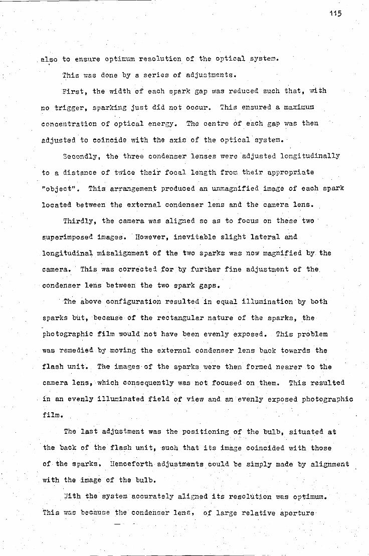
----------
also to ensure opti~um resolution of the optical system.
This was done by a series of adjuGtments.
First, the width of each spark gap was reduced such that, with
no trigger, sparking just did not occur. This ensured a maximum
concentration of optical energy. The centre of each gap was then
adjusted to coincide with the axis of the optical system.
115
Secondly, the three condenser lenses were adjusted longitudinally
to a distance of tl'lice their focal length fror:. their appropriate
"object". This arrangement produced an unmagnified image of each spark
located between the external condenser lens and the camera lens.
Thirdly, the camera was aligned so as to focus on these two
superimposed images. ·However, inevitable slight lateral and
longitudinal misalignment of the two sparks was now magnified by the
camera. This was correcte:i for by further fine adjustment of the
condenser lens between the two spark gaps.
The above configuration resulted in equal illumination by both
sparks but, because of the rectangular nature of the sparks, the
photographic film would not have been evenly exposed. This problem
was remedied by moving the external condenser lens back towards the
flash unit. The images· of the sparks were then formed nearer to the
camera lens, which consequently was not focused on them. This resulted
in an evenly illuminated field of view and an evenly exposed photographic
film.
The last adjustment was the positioning of the bulb, situated at
the back of the flash unit, such that its image coincided with those
of the sparks. Henceforth adjustments could be simply made by alignment
with the image of the bulb.
·~'ii th the system accurately aligned its resolut5.on was optimum.
This was becaune the condenser lens, of large relative aperture
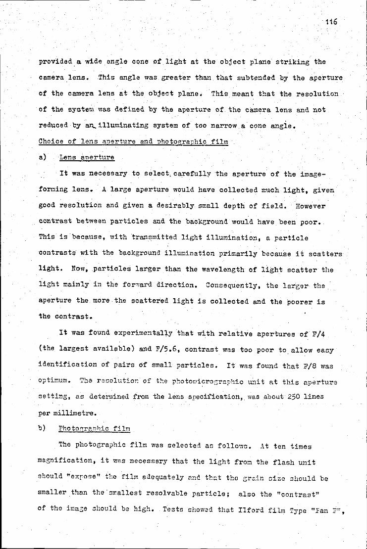
116
provided. a wide angle cone of light at the object plane striking the
camera lens. This angle was greater than. that subtended by the aperture
of the camera lens at the object plane. This meant that the resolution
of the system was defined by the aperture of the camera lens and not
reduced by an.. illuminating system of too narrow a cone angle.
Choice of lens anerture and nhoto~raphic film
a) Lens anerture
It was necessary to select, carefully the aperture of the image-
forming lens. A large aperture would have collected much light, given
good resolution and given a desirably small depth of field. However
contrast between particles and the background would have been poor.
This is because, with transmitted light illumination, a particle
contrasts with the background ill=ination primarily because it scatters
light. Now, particles larger than the wavelength of light scatter the
light mainly in the for-l'ard direction. Consequently, the lareer the
aperture the more the scattered light is collected and the poorer is
the contrast.
It was found experimentally that with relative apertures of F/4
(the largest available) and F/5.6, contrast was too poor to.allow easy
identification of pairs of small particles. It was found that F/8 was
optimum. Tl'l_a r-~solution of t!:e photorPi?ro.r;rnpbic u..~i t at this aperture
netting, as determinerl from the lens specification,. was ab cut 250 lines
per millimetre.
b) Photo~r~nhic film
The photographic film was selected as follows. ,\t ten times
magnification, it was necessary that the light from the flash unit
should "exro.<Je" the film adequately 11n<'. th::o.t the gr;;.:cn size :Jhould be
smaller t!:tan the'smallest resolvable particle; also the "contrast"
of the ima3e should be high. Tests showad that Ilford film Type "Fan
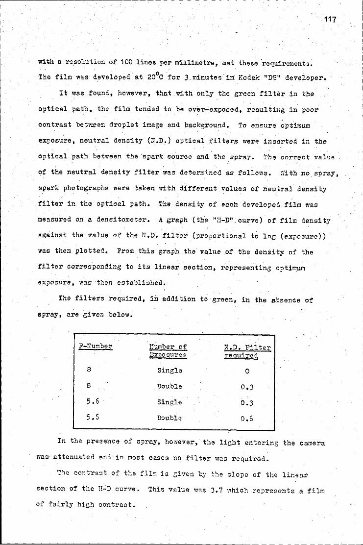
I
I
I
117
With a rs.solution of 100 lines per millimetre, met these 'requirements; 0 .
The film was developed at 20 C for 3 minutes in Kodak "D8" developer.
It was found, however, that with only the green filter in the
optical path, the film tended to be over-exposed, resulting in poor
contrast bet~en droplet image and background. To ensure optimum
exposure, neutral density (r! .D.) optical filters were inserted in the
optical path between the spark source a_11d the spray. T·he correct value
of the neutral density filter was determi.ned as follows. With no spray,
spark photographs were taken with different values of neutral density
filter in the optical path. The density of each developed film was
measured on a densitometer. A graph (the "H-D". curve) o:f' film density
against the value of the N.D. filter (proportional to log (exposure))
was then plotted. From this graph .the value of the density of the
filter corresponding to its linear section, representing optimum
exposure, was then established.
The filters required, in addi.tion to green, in the absence of
spray, are given below.
F-Number !lumber of N.D. Filter Ex:oosures reguired
.
8 Single 0
8 Double 0.3
5.6 Single 0.)
5.5 Double 0.6 .
In the presence of spray, however, the lir;ht entering the camera
was attenuated and in most cases no filter was required.
T~1e contraot of the fll!n is sive:1 by the slope of tho linear
section of the n.:D curve. This value was ).7 which repr.;centc a film
of fairly high contrast.
5.1.4 Constant temperature enclosure
The saturated vapour pressure of the propellant mixture varied • 2
by about 10 k:N/m ( 1. 5 p. s. i.) for a change of temperature of' one
degree C. It was essential, therefore, that the propellant temperature
was closely controlled.
The experimental apparatus was· contained in a laboratory held at
a temperature constant to within about.:!: 3 deg.C by thennostatically
controlled electric heaters. The section housing the propellant
cylinder and nozzles was held constant to within about.:!: 0.5 deg.C.
by an aluminium radiation shield and controlled by a contact thermometer.
Heat was distributed uniformly by a fan at the top of' the apparatus.
Variation in propellant temperature resulting from change of'
ambient temperature was thus minimised. It remained only to ensure
that the temperature of the .propellant in the container did not drop
significantly during spraying as a result of' evaporative cooling. The
permissible duration of spraying was estimated from the heat balance
given below.
Typical mass flow-rate = 3 x 10⁻³ kg/sec
Mean density of P 11/12 solution = 1 • 4 x 1 o3 kg/m 2
n " " vapour 2 = 6 kg/m
Mass of propellant in the container = 2 kg
Specific heat of the solution
Latent heat of·vaporisation
= 0.92 kJ/kgjdeg c.
= 170 kJ/kg
Therefore in ti~e t seconds,
the discharged propellant =
the volume of vapour produced to replace
3 x 1 o-3 t 3 m
1.4 X 10_3-
Therefore the mass of the vapour produced 6 kg
118
Therefore 3 X 10'"3t
1.4 X 10⁻³ 6x170kJ = 2 x .92 x (allowed temperature drop)
If the temperature <l.rop was to be less than 0.2 deg C, say, the
spray duration must be less than 200 seconds - providing the propellant
container is almost full. However, as the duration of the spray was
typically 30 sec, temperature fall <luring spraying could be neglected
until the container was almost empty.
5. f. 5 Sediroenta tion apparatus
In order to obtain a size analysis of the residual surfactant
spray, particles of the spray were collected on microscope slides
placed at the bottom of a cylinder of large dimensions referred. to in
119
Section 2. It consisted of a 600mm deep polythene container of diameter.
400mm equipped with a close fitting lid. Before each analysis 20 glass
microscope slides were cleaned in chromic acid, dried and placed at the
bottom of the container.
5,2 Calibration
5.2.1 The magnification of photomicrographic unit
The copying lens magnified nominally ten times. The precise
magnification was determined by photographing a ruled graticule,
placed accurately at the plane of focus of the image-forming lens.
5.2.2 The depth of field of the photomicrographic. unit
In order to determine the depth of field of the photomicrographic
unit, polydispersed aluminium powder, of mean diameter about 30.u m,
was photographed. The powder was first sprayed on to a microscope
slide, which was then positioned in the plane of focus of the image
o forming lens, but at an angle of about 80 to the optical axis of the
camera system. Single-flash photomicrographs were taken at varying
lens apertures, and prints of an overall magnification of 50 times were
obtained. Because the microscope slide was not normal to the optical
axis of the camera, a central band of particles only was in focus.
The width of this band was measured from the prints. The depth of
field was the.n obtained trigonometrically from the width of this band.
A graph of depth of field for a given lens aperture is given in Fig. 5.8.
5.2•3 Pressure gauges
During the course of the experimental programme two pressure
gauges of the Bourdon type (0- 345 kN/m2 or so·p.s.i.g.) were used •.
Each had a 150mm (6") dial and could be read to within.:!: 1.4 kN/m2
(0.2 p.s.i.). They were calibrated, using a mercury manometer, in an
orientation identical to that in use.
5.2.4.Thermocounles
The reference thermocouple was.placed in a Dewer flask of crushed
melting ice, frozen from distilled water. The thennocouple to be
calibrated was placed in a second Dewer flask containing distilled
water and a "Gold Line" thermometer graduated to 0.1 deg.C. The
calibration of this thermometer was checked at 0°C and 100°C.
The output of the thermocouples used on the continuous flow
apparatus were fed directly to the digital voltmeter, and a calibration
curve drawn. The resolution was 0.1 deg.C.
5.3 Exyerimental programme
As stated earlier, the purpose of the experimental programme was
to provide verification of theoretical expressions developed previously
and also to obtain empirical relationships relevant to ir~alation
therapy.
The theoretical expressions were developed to enable spray
120
characteristics to be determined in terms of the nozzle dimensions a.nd the
thermodynamic properties of the propellant only. It was found however that
additionally three empirical factors were required; they were the degree
of metastability of the propellant in the expansion chamber, the divergence·
angle and the position of the apparent origin of the spray. The first part
. .
600
500
~
e 400 ::>,. -0 .J llJ -IL 300
IL 0
:r 200 1-a. llJ 0
I 100
RELATIVE APERTURE ( F- NUMBER )
FIG.5.8. VARIATION OF· DEPTH OF FIELD OF THE CAMERA WITH APERTURE SETTING. ..... "' .....
122
of the experimental programme, therefore, included the measurement of the
three empirical factors. This information together with further data
constituted a means by which the theoretical expressions could be verified,
The second part of the programme was the measurement of size
distributions of the resultant surfactant aerosols generated by different
nozzle combinations,
It is appropriate, here, to review the derived expressions and explain
their relevance,
Initially, equations for the mass flow-rates through both upstream and
downstream nozzles were derived, By combining those two equations, the
temperature fall (and pressure fall) across the first orifice in terms of
the dimensions of the nozzle and the thermodynamic properties of the
propellant only were derived. It was necessary however to include, in
some cases, an empirical expression for the degree of metastability of
the propellant in the expansion chamber. From these expressions the mass
flow-rate could be determined, also in terms of fundamental parameters.
It was then possible to derive. an equation for the exit velocity
of the spray from the nozzle, From this exit velocity, together with
the previously derived mass flow-rate and the empirically determined
spray origin and d4vergence angle, the velocity of the gaseous componant
of the spray at a given point in the spray could be calculated. The .
velocity of the particulate componant of the spray could be determined
·from standard particle drag theory.
The above is necessarily an over-simplification and further details
are given in Section 6.
The experimental programme and the expression to which each part
of the programme relates are listed in the chart following,
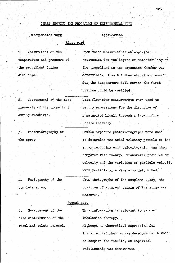
123
CHftRT SHO"'IING- THE PROG-RAMME OF EXPERIMENTAL WORK
Experimental work Application
First nart
1. Measurement of the
temperature and pressure a£
·the propellant during
discharge.
2. Measurement of the mass
flow-rate ot the propellant
during discharge.
From these measurements an empirical
expression for the degree of metastability of
the propellant in the expansion chamber was
determined. Also the theoretical expression
for the temperature fall across the first
orifice could be verified.
Mass flow-rate measurements were used to
verify expressions for the discharge of
a saturated liquid through a two-orifice
nozzle assembly. ----3. Photomicrography of
the spray
4. Photography of the
complete spray.
s. Measurement of the
size distribution of the
resultant solute aerosol.
. Double-exposure photomicrographs were used
to determine the axial velocity profile of the
spray,including exit velocity,which was then
compared with theory. Transverse profiles of
velocity and the variation of particle velocity
with particle size were also determined.
From photographs of the complete spray, the
position of apparent origin of the spray was
measured.
Second part
This information is relevant to aerosol
inhalation therapy.
Although no theoretical expression for
the size distribution was deve-loped \Vith which
to compare the results, an empirical
relationship v1as determined.
I . Experimental procedure
The propellant mixture used throughout consisted of, by weight,
60% of propellant 12,40% of propella:nt 11. Into this was dissolved 1%
124
by weight of the (liquid) surface-active agent .sorbitan trioleate ("Span 8.5")
. The propellant bottles, described in Sub-Section ,5,1, were filled with
propellant using a "cold -fill" technique in which both bottle and
propellant were first cooled in an isopropyl alcohol (IPA) refrigerator.
The propellant was then poured directly into the bottle. Atmospheric
water vapour, which may have c.ondensed on to the inside of the bottle,
was tht.is prevented from doing so by a blanket. of IPA vapour covering
the refrigerator.
After each bottle had been filled, the lid was screwed on and then
vapour was vented to remove any air from the bottle. This method had
an advantage over pressure injection filling, in that the amount of
air finally dissolved in the propellant was kept to a minium.
Before each run, the apparatus was allowed sufficient time to . 0
acquir~ a steady temperature, nominally 20 C. Immediately before the
run, the bottle was shaken to ensure that the propellant and surfactant
.were thoroughly mixed,
Each part of the experimental programme, given in the chart above,
will now be considered,
Measurement of the temperature and pressure in the expansion
chamber of the nozzle
Measurements of the temperature and pressure in the expansion
chamber were made for the nine nozzle combinations given in Section 6,
For each nozzle combination the pressure and temperature of the
propellant in the feed-pipe was checked and recorded before spraying,
to ensure that correct thermal conditions had been acquired. This was
done by reading, respectively, pressure gauge 1 and thermocouple 1,
situatedas shown in Fig. 5.1. The spray wes then discharged and
the data-logger started,
During spray discharge, the e.m.f.'s of the thermocouples 1, 2
125
and 3 were recorded automatically by the data logger, whilst the
steady-state·~eadings of pressure gauges 1 and 2 were recorded manually.
It was found that pressure gauge 1 quickly became steady at a value
slightly below its initial (no spray) value. Pressure gauge 2, however,
~ose quickly from zero to an inte~ediat~ value but then continued to
rise slowly, reaching steady-state conditions after about 10 to 15 seconds,
It was this steady-state reading of gauge 2 that was recorded.
The temperatures of the propellant either side of the first orifice
were obtained from a print-out of the data-loe;,ser tape. A typical er<> ph,
showing the variation of these temperatures with time, is shown in
Fig. 5.9. The steady-state reading of thermocouple J was recorded.
r.~nss flow rate
The apparatus was allowed to reach the steady temperature of the
constant~temperature enclosure. The spray generator, that is container,
feed-pipe and nozzle, was then tra.'lsferred to a stand placed on a direct
read-out balance. ·The configuration of the spr2y generator on the
stand was maintained the same as that on the spray rig, except that,
for convenience, the nozzle was positioned to spray horizontally.
The spray VID.S then started and :;-hen steady-state conditions· had
been reached, the time taken for 20,0gm to discharge, was measured
1."/i th a stop-watch. Three such rcac't.ings were taken, and the mean
calculated.
Afterwards, the spray generator was returned to the constant-
ter:;pernture e!1Closurc, the nozzle charlt;ed, and the procedure repeated.
"Photonic:ro.O'ranhv
Double-expocure anu,~or re~erence purposes,single-exposure
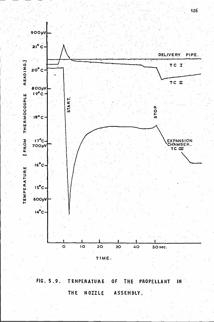
126
21° c DELIVERY PIPE. - . .
\!) TC r z 20°C -0 < w
TC II a: SOOpV
w 19°C ..J .-: a. ::) er 0 < a. 1-CJ li) 0 0 1-~ 18°C li)
a: Ill :t ....
~ 17°C EXPANSION 0 700pV CH'AMBER. et TC·m 1&.
""------
16°C w er ::) .... < a: 15°C w a. J1 w ....
14°C
0 10 20 30 40 sos~c.
TIME.
FIG. 5.9. TEMPERATUIH OF THE PROPELLANT IN
THE NOZZLE ASSH1BLY.
photomicrographa were taken of the emerging spray. The double-exposure
photographs were taken to determine:-
a)· the exit velocity of the spray from the nozzle.
b) the longitudinal velocity .along the spray axis,
and c) the transverse profile of longitudinal velocity in a plane
containing the spray axis.
The nozzle combinations used. and the parts of the spray which
were photographed are given in Section 6,
From the double-exposure photographs taken at a given point in the
spray, an accurate value of the velocity of particles at that point
was required, However as a spray is· in general a turbulent system,
velocities measured at a given positi~n.but at different times, vary
considerably. Tl:erefore, a time-average must be obtained. In order
to get an accurate time-average, a number of photographs must be taken
at a given point, this number depending on the accuracy required and
the degree of turbulence within the spray.
TO estimate the number of photographs required, let it be assumed
that there is to be a 90% probability that the sample time-averaged
velocity, obtained from N photographs, should be within 10% of the
long-term time-averaged velocity ( ii ). Then, assuming a normal
distribution of instantaneous velocities (with standard deviation s),
1,6 standard errors of the distribution of time-averaged velocities
( 45 ) should be less than or equal to 10% of the time-averaged
velocity.
Therefore:- 1.6s / .[N ~ (10/100) ii
or, N ;;;;: (16)2 (s/ ii)2
127
Here, s/ ii is the relative turbulence, an estimate of which woul~ enable·N
to be calculated, Initial experimentation showed that the relative turbulence,
----~------------------------------------------------~--------------------~-----
although varying with position in the spray, was typically 0.2, a
figure in agreement with reported values ( 66 ).
Insertion of this figure into the above equation leads to a value
of tan for the required number of double-exposure photographs. However,
the time required to take and analyse this number of photographs at
128
many positions within a large number of sprays would have been prohibitive.
Consequently, this criterion was relaxed to an extent depending on the
situation, as discussed in Section 6. Inevitably, a lar~er error in the
estimate of the average velocity was therefore incurred.
That so many photographs are required to obtain an accurate value
of the average velocity within a turbulent system is seen to be a
serious disadvantage of this method of velocity measurement. For example,
to ensure a 90% probability of incurring an error of no greater than
1% would require the analysis of about 1000 double-exposure photographs.
Method
The part of the spray first to be photographed was usually an axial
point olose to the exit of the nozzle. The latter was first iowered
and adjusted transversally until it appeared in the field of view of
the camera. So that the camera could be focused precisely on the spray
axis, the latter was first defined by a jet of water. To do this,
the water was injected, at moderate pressure, through the "T" piece
provided in the feed-pipe. It then emerged as a continuous jet along
the .spray axis, providing a suitable object on which to focus the
camera.
The propellunt was then discharged. 'ilhen bubbles were seen to
have cleared from the perspex tube above the first orifice, and steady-
state conditions had been reached, photographs were taken of the spray.
To photograph other axial positions within the spray, the nozzle
was raised relative to the camera. It was necessary, after raising
~----------------~----------------------------------------~---- -
I I I I I I
- __ _j
the nozzle, to check that the spray axis still passed through the
object plane of' the camera and use was again made of' the water jet.
To obtain photographs of' off-axis positions in the spray, the
nozzle was moved transversely relative to the camera.
5.4;:4 Photogranhy of the complete spray
129
In order to obtain a direct measure of the apparent position· of the
origin of the spray, photographs of the complete spray were taken. By
setting a 35mm. camera about 1 metre·from the spray, which was illuminated
with flood lights, photographs of' 500mm length of the spray were obtaineJ.
From these, the position of the spray origin could be measured. Half
microsecond flash photographs were also taken.
5.4.5 Size analysis of the resultant aerosol of surface-active
solute.
TWerity microscope slides were cleaned, dried and placed at the
bottom of the sedimentation cylinder which was placed beside the spray
rig. After the latter had ac~uired a steady temperature, the nozzle
was removed from its mounting and the spray discharged, After steady
state conditions within the nozzle had been reached, the spray was
directed into the sedimentation cylinder for about two seconds. This
length of time was found to be optimum; a shorter spraying time
resulted in too few droplets on the slides, whilst a longer time
resulted in overlapping of the droplets.
· The nozzle was then directed away from the column ar.d spraying
stopped. The lid of the sedimentation cylinder was then replaced,
The resultant aerosol was allowed to sediment for fifteen hours
on to the twenty glass slides which were then removed from the cylinder.
The size distribution was obtained by microscope analysis using
a techni~ue first described by May ( 39 ). The procedure is. described
briefly beJ.orr.
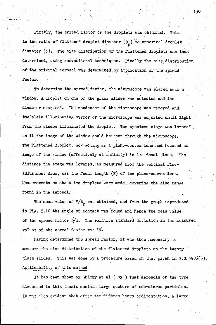
Firstly, the spread factor or the droplets was obtained. This
is the ratio. of flattened droplet diameter (D) to spherical droplet p .
diameter (d). The size distribution of the flattened droplets was then
determined, using conventional techniques. Finally the size distribution
of the original aerosol was determined by application of the spread
factor.
To determine the spread factor, the microscope was placed near a
window. A droplet on one of the glass slides was selected and its
diameter measured. The condenser of the microscope was removed and
the.plain illuminating mirror of the microscope was adjusted until light
from the window illuminated the droplet. The specimen stage was lowered
until the image of the window could be seen through the miorosc.ope.
The flattened droplet, now acting as a plano_;conve:x: lens had focused an
image of the window (effectively at infinity) in its focal plane. The
distance the stage was lowered, as measured from the vertical fine-
adjustment drum, was the focal length {F) of the plano-conve:x: lens.
Measurements on about ten droplets were made, covering the size range
found in the aerosol.
The mean value of F/Dp was obtained, and from the graph reproduced
in Fig. 5.10 the angle of contact was found and hence the mean value
130
of the spread factor D/d. The relative standard deviation in the measured
values of the spread factor was 4%.
· Having determined the spread factor, it was then necessary to
measure the size distribution of the flattened droplets on the twenty
glass slides. This was done by a procedure based on that given in B.S.3406(5).
Applicability of this method
It has been shovm by '.'1hitby et al ( 72 ) that ·aerosols of the type
discussed in this thesis contain large numbers of sub-micron particles.
It was also evident that after the fifteen hours sedimentation, a large
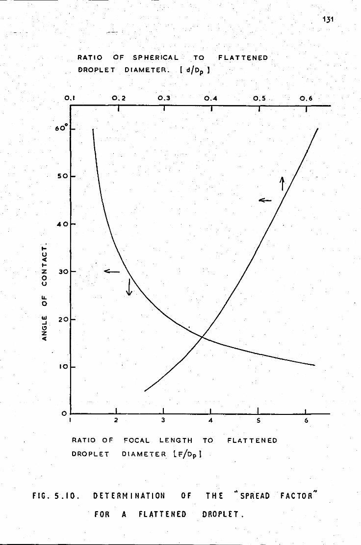
131
RATIO OF SPHERICAL TO FLATTENED
DROPLET DIAMETER. ( d/Dp)
0.1 0.2 0.3 0.4 0.5 0.6
so
40
1-u <(
1-z 30 0 u
lL 0
ILl 20 ...1 C) z <(
10
oL-------L-------~------~------~------~~--1 2 3 4 5 6
RATIO OF FOCAL LENGTH TO FLATTENED
DROPLET DIAMETER lFjDp)
FIG. 5.10. DE TERM I NATION OF THE "SPREAD " FACTOR
FOR A FLATTENED DROPLET.
number of particles remained in the sedimentation chamber. This
could je demonstrated by directing a beam of light from a microscope
la.t:F tin-ough the chamber. A vast number of particles were observed in
the oe!l!ll. Application of Stoke's Law indicated that the diameters of
thes-; :i:roplets were less than 0. 71Jm .
132
.!t would have been meaningless, therefore, to calculate a mean
diarof:t~r which was sensitive to the large number of sub-micron particles.
Homns:-, it was sh01m earlier that the information required from the
size •listributions was the fraction by volume of particles below a particle
di.a:>n,·r of approximately 51Jm. For the aerosols of interest, generated
fro~ saturated liquids, the fraction by volume in the sub-micron region
wili. 'oe negligible compared with that below 5 1J m. Therefore the size
di£'.c·:'.C?utions will be meaningful , despite the omission of the sub-micron
6 . EXPERI!.lENT.AL RESULTS AND COMPARISON WITH THEORY
6.1 Determination of the values Of the constants C1, C2
, c3
andy.
6.2. Measurement of mass flow-rate and comparison with theoretical
expressions for the flow-rate through a single.orifice.
Determination of discharge coefficients.
133
6.3 Measurement of the temperature fall,LlT1 across the first orifice
of the nozzle assembly and comparison with theory~
6.4 Experimental verification cf the expression for the mass flow-
rate through a two-orifice nozzle assembly.
6.5 Measurement of the relative velocity between liquid and gas
phases at the exit of the nozzle.
6.6 Measurement of the exit velocity of the spray and comparison
with theory.
6.7 Measurement of the transverse profile of longitudinal velocity
within the spray.
6. 8. Measurement of the divergence anele of the spray.
6.9 Measurement of the longitudinal profile of longitudinal
velocity within the spray and comparison with theory.
6.10 Measurement of the variation of particle velocity within
a sp~y with particle size, and comparison with standard theory.
6.11 Determination of the size analyses of the resultant surfactant
aerosols and their variation with nozzle dimensions,
6.12 Deteruination of the deeree of metastability of the propellant
in the expansion chamber,
In Section 4 an expression was produced by which the loneitudinal ,_,
velocity profile •vi thin a continuous spray could be predicted, A
double-flash photomicrograph of' such a spray is shown in Fig. 6.1.
In this section the quantitative predictions of each step in
the development of the above expression are presented and C9mparisons
are made vdth the experimental results. The verification
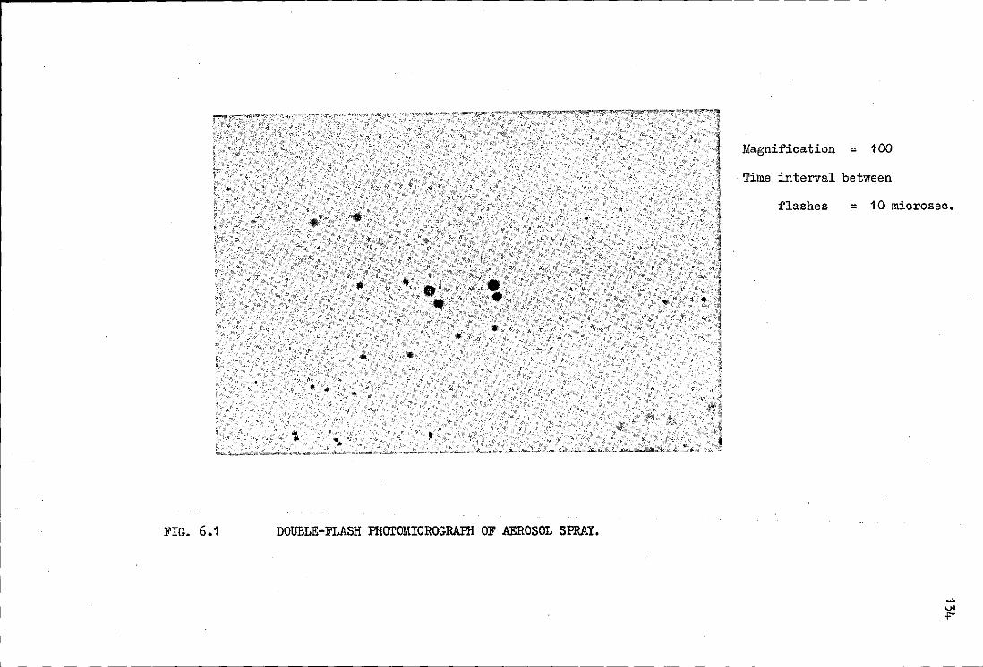
Magnification = 100
Time interval between
flashes = 10 microsec.
FIG. 6.1 DOUBLE-FLASH PHOTOMICROGRAPH OF .AEROSOL SPRAY.
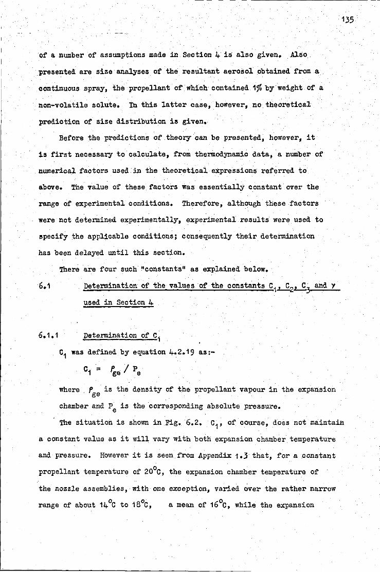
of a number of assumptions made in Section 4 is also given. .Also.
presented are size analyses of the resultant aerosol obtained from a
continuous spray, the propellant of which contained 1% by weight of a
non-volatile solute. In this latter case, however, no theoretical
prediction of size distribution is given.
Before the predictions of theor,y can be presented, however, it
is first necessary to calculate, from thermodynamic data, a number of
numerical factors used in the theoretical expressions referred to
above. The value of these factors was essentially constant over the
range of experimental conditions. Therefore, although these factors
were not determined experimentally, experimental results were used to
specify the applicable conditions; consequently their determination
has been delayed until this section.
There are four such •constants" as explained below.
6.1 Determination of the values of the constants c 1~~3 and y used in Section 4
6.1.1 Determination of c1
c1 was defined by equation 4.2.19 as:
C1 = fge / pe
where . p is the density of the propellant vapour in the expansion ge
chamber and Pe is the corresponding absolute pressure.
135
The situation is shown in Fig. 6.2. c1, of course, does not maintain
a constant value as it will vary with both expansion chamber temperature
and pressure. However it is seen from .Appendix 1·.3 that, for a constant
propellant temperature of 20°C, the expansion chamber temperature of
the nozzle assemblies, with one exception, varied over the rather narrow
0 0 range of about 14 C to 18 C, a mean of 16°c, while the expansion
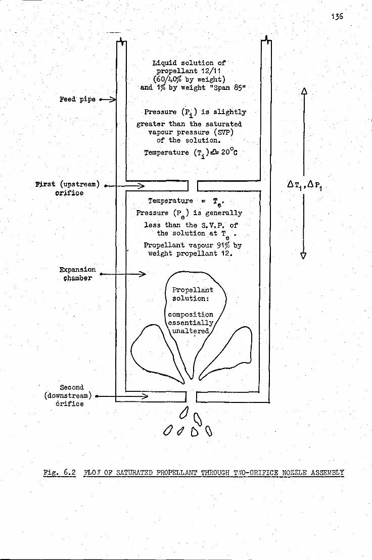
Feed pipe
Liquid solution of propellant 12/11
(60/4fY% by weight) . • and 1% by weight "Span 85"
Pressure (Pi) is slightly
greater than the saturated vapour pressure (SVP)
of the solution.
Temperature (T.) .!l= 20°C l.
nrst (upstream) -t~~~===J orifice -
Temperature = T6
•
Pressure (P ) is generally e less than the S.V.P. of
the solution at T • e
· Propellant vapour 91% by weight propellant 12.
Expansion ._-t-f~~ cn~ber
Propellant solution:
composition essentially Wlaltered
Second
{downstream) •-{~=~====:] orifice
a~ 017'D'0
136
Fig. 6.2 FLO.V OF SATURATED PROPELL.ANT THROUGH TNO-ORIFICE NOZZLE ASSEMBLY
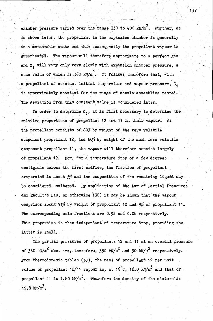
chamber pressure varied over the range 330 to 400 kN/m2• Further, as
is shown later, the propellant in the expansion chamber is generally
in a metastable state and that consequently the propellant vapour is
supsrheated. The vapour will therefore approximate to a perfect gas
and c1 will vary only very slowly with expansion chamber pressure, a
mean value of which is 360 kN/m2• It follows therefore that, with
a propellant of constant initial temperature and vapour pressure, c1
is approximately constant for the range of nozzle assemblies tested.
The deviation from this constant value is considered later•
ID order to determine c1, it is first necessary to determine the
relative proportions of propellant 12 and. 11 in their vapour. As
the propellant consists of 60}1, by weight of the very volatile
componant propellant 12, and 40% by weight of the much less volatile
componant propellant 11, the vapour will therefore consist largely
of propellant 12. Now, for a temperature drop of a few degrees
centigrade across the first orifice, the fraction of propellant
evaporated is about 5% and the composition of the remaining liquid·may
be considered unaltered. By application of the Law of Partial Pressures
and Raoult's Law, or otherwise (30) it may be shown that the vapour
comprises about 91% by weight of propellant 12 and 9% of propellant 11.
The corresponding mole fractions are 0.92 and 0.08 respectively.
This proportion is then independant.of temperature drop, providing the
latter is small.
137
The partial pressures of propellants 12 and 11 at an overall pressure
of 360 kN/m2 abs. are, therefore, 330 kN/m2 and 30 kN/m2 respectively.
From thermodynamic tables (30), the mass of propellant 12 per unit
volume of propellant 12/11 vapour is, at 16°C, 18.0 kN/m3 and that of
propellant 11 is 1.80 kN/m3• Therefore the density of the mixture is
19.8 kN/m3•
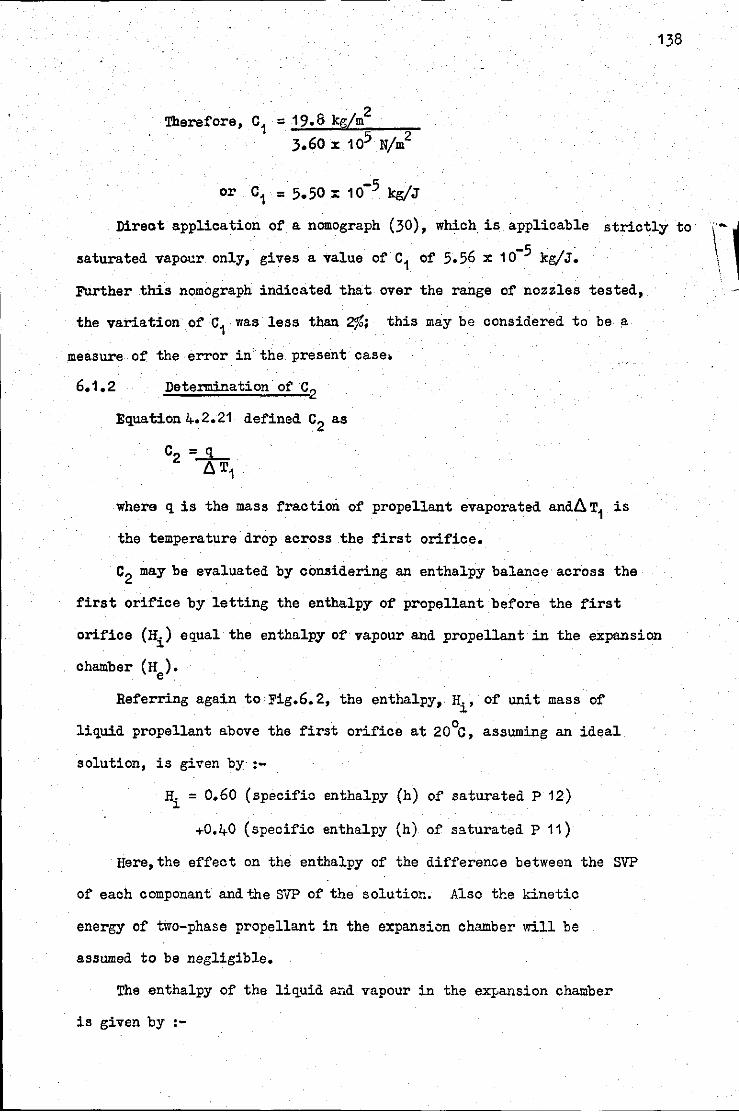
138
Therefore, c1
or . c1 = 5.50 ::: 1 o-5 kg/J
Direct application of a nomograph (30), which. is applicable strictly to
saturated vapour only, gives a value of c1 of 5.56 x 10⁻⁵ kg/J~
Further this nomograph indicated that over the range of nozzles tested,
the variation of c1 was less than 2%; this may be considered to be a
measure of the·error in.the present case.
Determination of c2
where q is the mass fraction of propellant evaporated and~T1 is
the temperature drop across .the first orifice.
c2 may be evaluated by considering an enthalpy balance across the
first orifice by letting the enthalpy of propellant before the first
orifice (Hi) equal the entho.lpy of vapour and propellant in the expansion
chamber (He).
Referring again to Fig.6.2, the enthalpy, Hi' of unit mass of
liquid propellant above the first orifice at 20°C, assuming an ideal
solution, is given by· :-
Hi = 0,60 (specific enthalpy (h) of saturated P 12)
+0.40 (specific enthalpy (h) of saturated P 11)
Here,the effect on the enthalpy of the difference between the SVP
of each componant and the SVP of the· solution. Also the kinetic
energy of two-phase propellant in the expansion chamber will be
assumed to be negligible,
The enthalpy of the liquid and vapour in the ex~ansion chamber
is given by :-
··-\ \
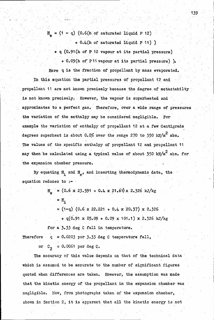
He = (1 - q) (0.6(h of saturated liquid P 12)
+ 0.4(h of saturated liquid P 11) )
+ q (0.91 (h of P 12 vapour at its partial pressure)
+ 0.09(h of· P11 vapour at its partial pressure) ),
Here q is the fraction of propellant by mass evaporated,
In this equation the partial pressures of propellant 12 and
.propellant 11 are not known precisely because the degree of metastabilty
is not known precisely. However, the vapour is superheated and
approximates to a perfect gas, Therefore, over a wide range of pressures
the variation of the enthalpy may be considered negligible. For
example the variation of enthalpy of propellant 12 at a few Centigrade
degrees superheat is about 0,8% over the range 270 to 350 kN/m2· abs.
The values of the specific enthalpy of propellant 12 and propellant 11
may then ·be calculated using a typical value of about 350·kN/m2 abs, for
the expansion chamber pressure,
By equating H. and H , and inserting thermodynamic data, the 1 e ·
equation reduces to :-
H . = (0,6 X 23,591 + 0,4 X 21,61) X 2.326 kJ/kg e .
=Hi
= (1-q) (0,6 X 22,221 + 0,4 X 20,37) X 2.326
+ q(0,91 X 85,09 + 0,09 X 101,1) X 2,326 kJ/kg
for a·3.33 deg C fall in temperature.
Therefore q = 0.0203 per 3.33 deg C temperature fall,
or c2 = 0, 0061 per deg C.
The accuracy of this value depends on that of the technical data
which is assumed to be accurate to the number of sienifica.'lt f'igures
quoted when differences are taken, However, the assumption was made
that the kinetic energy of the propellant in the expansion chamber was
negligible, Now, from photographs taken oi' the expansion chamber,
shown in Section 2, it is apparent that all the kinetic energy is not
139
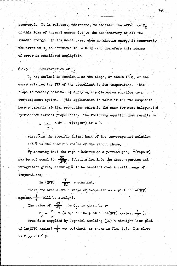
recovered. It is relevant, therefore, to consider the effect on c2
of this loss of thermal energy due to the non-recovery of all the
kinetic energy. In the worst case, when no.kinetic energy is recovered,
the error in c2 is estimated to be 0,7%, and therefore this source
of error is considered negligible.
6.1.3 Determination of c3
c3 was defined in Section 4 as the slope, at about 18°C, of the
curve relating the SVP of the propellant to its temperature. This
slope is readily obtained by applying the Clapeyron equation to a
two-componant system •. This application is valid if· the. two compnants
have physically similar properties which is the case for most halogenated
hydrocarbon aerosol propellants.. The following equation then results :
- _!_ ~ dT + v(vapour) dP = O,
T
where 'A is the specific latent heat of the two-componant solution
and v is the specific volume of. the vapour phase.
By assuming that the vapour behaves as a perfect gas, v(vapour)
may be put equal to (~J· Substitution into the above equation and
integration gives, assuming A to be constant over a small range of
temperatures,:-
ln (SVP) = + constant.
Therefore over a small range of temperatures a plot of ln(SVP) . 1
against ~ will be straight.
The
From
dP value of ~ , or c3
, is given by :-
c3 = : 2 x (slope of the. plot of ln(SVP) against + ). data supplied by Imperial Smelting (30) a straight line plot
of ln(SVP) against + was obtained, as shown in Fig •. 6.3. Its slope
is 2.33 x 1aJ x.
140
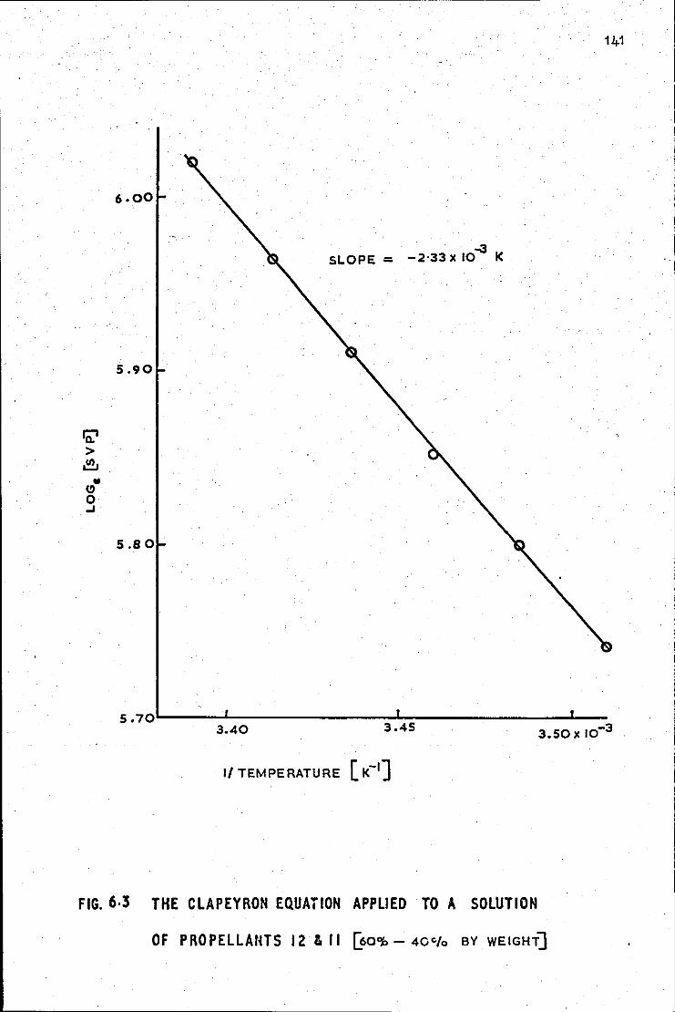
ra: > ~ .. ~ 0 ..J
6.00
5.90
5.8 0
..,'3 SLOPE= -2·33xl0 K
141
5.70~----~--------------~~--------------~---3 .45 3.50 X 10⁻³ 3.40
1/ TEMPERATURE [K-1]
FIG. 6·3 THE CLAPEYRON EQUATION APPLIED TO A SOLUTION
OF PROPELLANTS 12 & 11 [60~-40°/o BY WEIGHT]
Now, at 18°C the S.V.P. is 370 kN/m2 •
Therefore _c3
= 370 .x 2.33 x 1o3 = 10,1 kN/m2/deg C,
(291)2
The inherent accuracy of this figure again depends on the accuracy
of the technical data and is thus expected to be adequate, However
errors occur if the temperature varies about a mean other than 18°c. 2 .
For example c3
determined at 16°C is 9. 70 kN/M /deg c, an error of 4%.
In such a case therefore it would be desirable to use the new value
Determination of y
In equation 4.2.11 it was shown that the value of 'Y, the ratio
of the specific heats of the propellant 12/11 vapour was required at
the point of choking. · It has been assumed that at the point of choking
the following conditions prevail :-
1, The pressure is given by:·
142
{critical pressure ratio, 0.52 ) x (expansion chamber pressure)
2. The fractions by weight of propellants 12 and 11 at the point
of choking are equal to those. within the expansion chamber.
This is because it is assumed that no mass (or heat) transfer
takes place·during the passage of the propellant through the
orifice, These fractions are approximately 0.9 and 0,1
respectively,
3, The temperature
By definition: y
It is therefore necessary to determine vaiues of CP and CV under
conditions defined above.
As y is a slowly varying function, typical values of critical
I I I I '
143
conditions may be used. A typical value of the expansion chamber
pressure is 350 kN/m2 acs. Therefore the pressure at the point of choking
is .52. x 350 or 180 kN/m2• A .typical value of the expansion chamber is
17°C. Therefore the temperature of the vapour. at the point of choking
is given by :-
As the value of y is required before T0
can be determined, an iterative
mathematical process is necessary, The last stage of this is that an
approximate value for of 1.16 gives a. value.of -9°C for the temperature
of the vapour at the point of choking.
By definition:-
= ( a H ) cP aT P
and a s ) = T( a T V' or, more conveniently
CV = Cp - T ( ( : ~ )p ( ~ ; )T )
From thermodynamic tables for propellants 12 and 11
the following ma.y be obtaine.d :-
For propellant 12 under the conditions stated:-
cp = 0.605 kJ/kg/deg c
cP- cv = o.OB9
Therefore. CV = 0.516
"
"
For propellant 11 under the same conditions:-
cp = 0.531 kJ/kg/deg c
cP- cv = o.63
Therefore CV = 0.468
"
" Therefore = 0.9 x 0.605 + 0.1 x·0.531
0.9 X 0.516 + 0.1 ·X 0.468
or 1.17 •
,
The accuracy of this value is dependant on the confidence with which
"--------------'---------·-- ·- -
the conditions at the point of choking are defined, An error arises
if the assumption that no heat transfer takes place during the
passage of the propellant through the. orifice is wrong. In the worst
case of rapid heat transfer, such that the gas remains at expansion
chamber temperature during the passage through the. orifice, y would
take a value of 1,15 •
•
144
6.2 Measurement of mass flow rate and comparison with theoretical
expressions for the flow rate through a single orifice.
Determination of the discharge coefficients of the upstream
and downstream orifices of'. the nozzle assembly, cQ1 and CQ2
respectively.
In Section 6.1, four quasi-constant parameters were determined
from thermodynamic data. As explained in the introduction, it is now
possible to present experimental verification f'or the various steps
in the development of a fundamental expression fo~ velocity profiles
within a. spray. The f'irst step in this development was to equate
an expression for the mass ·f'low-rs.te through the upstream orifice to
.that for the downstream orifice, thus producing an equation for the
temperature fall~T1 across .the first orifice. It is therefore first
necessary to verify each cf these two expressions for the mass flow-
rate. This may be done by following standard fluid dynamics practice
which is to demonstrate that over a wide range of conditions the
discharge coefficient of the orifice is constant and approximately
equal to 0.83, a value determined independently in Appendix 3.
6.2.1 Determination of the discharge coeff'icient of the upstream
orifice, cQ1
· It is anticipated that the upstream orifice passes the propellant
in the liquid phase. This follows partly from Pasqua's criterion ( 50 )
145
described in Section 2, which states that a saturated liquid, ·discharging
through a short tube, will not exhibit choking effects providing the
downstream predsure is greater than :-
( ) (Length of tube) 0.2 0.37 x initial saturation pressure -Dia. of' tube
. 2 Now, in this work the initial saturation pressure was 400 ~/m abs.
and the length of each orifice was approximately equal to its diameter.
Therefore, for a do1mstream (expansion chamber) pressure of greater than
Wi. 2 . .
0.37 X 400 or 150 kN/m abs. no choking effects are expected. Reference
to Avpendix 1.3 shows that in all cases the expansion chamber pressure . 2
greatly exceeded. 150 kN/m abs.; the lowest value wa.s 244 kN/m2 abs. Further,
the propellant at the first orifice is sub-cooled by a half,-metre head of
propellant. Consequently, it is considered that the standard expression for
the discharge of a single-phase incompressible fluid may be used to define
CQ1• This was given in equation 4.2.1 as:-
Jr-2-1'-'1-(P_i ___ p e-)-( iT
4
If this equation is valid then a plot of against
J (Pi - Pe)
CQ1~
for all nozzle assemblies will be linear, and equal to
Fig. 6.4 shows the above plot obtained from data given in
Appendices 1.2 and. 1 .3.
It can be seen that the plot is reasonably linear, with a slope of
41.4 (kgjm3 )"~·. As the density of the propellant, p1
, is 1.40 x 1o3 kgjm3,
cQ1
= 0.78. Further, as the plot is linear, support is given to the
assumption that the propellant remains a liquid during its passage through
the upstream orifice.
The possible error associated with these data points may next be
considered. The most likely source of error is that due to non-uniformity
along the diameter of the orifices; In the worst case this could cause
an error of about 4% in the determination of the area of the orifice.
The two other sources of error, those associated with the measurement
• of the mass flow rate (M) and the pressure differential across the first
orifice ~P1 ), are generally smaller than 4%, as is seen from Appendices
1.2 and 1.3 .This is not the case however when the pressure differential
is small. Thus the departure from linearity cf the data point for nozzle
0.65 x 0.35 is attributed. to this latter source of error. The other data
points are within about 4% of the regression line.
147
I'll 18 X 103
'e NOZZLE i'u
/320x?OO .. Ul
"' "" Ul
I 5 I 0 u. a: 0
I :I <( 450 X 700 Ul a:
I 320 X 450 ,...
Ill 250 X 350 0..
~ V
T J: 10 ,Q/ 320 X 350 (!) ~ 0 a: J:
450 X 450 ,...
I <( 680 X 700 Ul a: c(
,... z 640 X 450 ~
a: Ul 5 0.. 640 X 350
Ul ,... <(
a: ;;:: 0 ..J u.
Ill Ill <(
:I
5
j PRESSURE DIFFERENTIAL ACROSS THE UPSTREAM ORIFICE
FIG. 6.4. DISCHARGE OF PROPELLANT THROUGH THE
UPSTI\EA M ORI Fl CE.

The linearity of the regression line and the good agreement between
the measured discharge coefficient and the expected value is taken to
confirm the applicability of the above expression (equation·4;2,1).
6.2.2 Detennination of the discharge coefficient of the downstream
orifice, cQ2
It has been shown that unlike the upstream orifice, the downstream
orifice discharges a two-phase fluid - the liquid propellant and its
vapour, In Section 4 two expressions were developed for the discharge
of such a fluid, one for a low pressure differential. across the orifice
and the other for a large pressure differential which would be expected
to create choking or mass-limiting effects within the orifice, A probable
criterion for mass-limiting flow is that the ratio of downstream (ambient)
pressure to upstream (expansion chamber) pressure should be less than
about 0,5 , Reference to Appendix 1.3 shows that in all cases this
ratio is less than 0,52, the largest value being 0.42. It is therefore
to be expected that the second expression, which includes the effects
of mass-limiting flow, would be applicable. This expression was given
by equation 4,2,14 as:-
( 1
)2 ,
in which the variables are as defined in Section 4 and refer
to the point of choking,
Now it was sho~n subsequently that the following substitutions
could be made in order to transform the equation into a more amenable
form :-
q = c2 t. T1'
P = r P c c e ,
- -----·-·
p 1
l'gc = ~e (~)--:;- , and Pe
fge = c Pe' and that therefore, 1 1
f'gc = c1 p r i' e c
Substitution into the above gives :-
= ')' + 1
r 2y c
The coefficient of cQ2 Pe /JD.T1 on the right hand side of the
above is essentially constant over the range of operating conditions.
Therefore a linear relationship between M/((rr/4)D22
) and Pe /jD.T1,
and a value of cQ2 again approximately equal to 0.8 would be taken as
support for the applicability of the above expression. Fig. 6.5 shows
this relationship. It is seen that of the nine data points, six fall
on a reasonably straight line while three depart significantly from this
line. Of these three, the data from nozzle 650 x 350 could be in error
because the value of the temperature differential (D. T1) is small.
This is not the case however with the other two. A possible source of
error in the data from these two·nozzles is that the physical conditions
within the nozzle were not typical of the conditions for which the values
of c1
, c2
, c3
andywere determined (this, of course, applies to any
nozzle). However,both nozzles have orifice pairs which are of similar
diameter and consequently the conditions within those nozzles are
fairly typical. Perhaps in view of the number of assumptions made in
the development of the mass-limiting flow - rate equation, and its
simplicity in describing the mass flow-rate per unit area of two-phase
flow in terms of a pressure(that within the expansion chamber), a
temperature differential(t~~t across the first orifice) and a quasi-·
constant factor, then the correlation between theory and experimental
149
N 'e i"u .. .. j
111 I 5 u u. 0:: 0
:I < Ill 0::
~ z ;;: 0 Q 10
u. 0
< Ill
~ 1-
z :I
0:: Ill D..
Ill 1-< a: ;;: g u.
Ill Ill < :::!:
5
I /
I ·"1("1 (q . Q ....
I I
0
0
1.0 2.0 3.0
EXPANSION CHAMBER PRESSURE
JTEMPERATURE FALL ACROSS UPSTREAM
NOZZLE.
640 X 320 0
640 X 450
450 X 450
320 X 350
690 X 700
320 X 450 250 X 350
450 X 700
320 X 700
4.0 5
5.0 X 10
FIG. 6. 5. DISCHARGE OF. PROPELLANT THROUGH THE
DOWNSTREAM ORIFICE. [FOR CHOKING FLOW]
150
151
data may be considered satisfactory. Further discussion of the.
applicability of the mass~limiting flow-rate equation is given in later
sub-sections.
Accepting, tentatively, that this equation describes reasonably well
the masa flow-rate of a two-phase fluid, then from the regression line
·Of Fig. 6.5 a value for the discharge coefficient of the orifice may be
determined. This is :-
CQ2 = O. 78.
This is in good agreement with that obtained fron single-phase flow,
thus further supporting to the applicability of equation 4.2.14.
It is instructive. to compare, with experimental flow-rate data,
not only the prediction of mass-limiting flow theory (equation 4.2.14)
but also that of non mass-limiting flow theory. This was expressed in
equation 4.2. 8 as follows :-
M:2 = CQ2 (n/4) D2 2 fa uo '
where f is the density of the two-phase fluid at the nozzle 0 .
exit and u is the corresponding velocity. 0
f. is given by:o
1
fo =
q
and u0
is given by :-
•
=
1 q p y
(Pe - P amb) + -fg_e....:C;-1-_--..,.1...,) 'Y
(P 1 e
1 y
1 1 - -:;;') ,
pamb '
where the variables are as defined in Section 4 •.
As with the previous equation substitutions may be made. These are:-
q = c2 tlT1, fge = c1 p and e
p b 1 p 1
1 1 -- Pamby ~0 = fge (~-)Y = c1 y . pe e
152
Equation 4,2.8 then· reduces to ·-
•
[ CQ2 ),{2 =
(1T/4) D 2 c2 t1T1 2
c p 1 1 e
t -C t1T :z: 2 1 (P _ p )
f. e amb l.
[2
1 y
1
pamby
1 c (1 - -) 1 y
+ 1 - c2 1:1 T1
fl
p 1 (1 -( a.mb )
Pe
This equation again incl.udes only two variables, They are the
J
_.! y
)
expansion chamber pressure, P , and the temperature ~all across the ~irst e
ori~ice, 1:1 'f1, The other parameters are either constant or quasi-constant.
However the equation is seen to be more complex than that incorporating
mass-l.imiting ~low,
Fig 6.6 shows a plot o~ the mass ~low-rate per unit area against
the theoretical expression given by equation 4,2,8 above, It is seen
that, rather surprisingly, agreement is better than in the previous" case-
r
in particular the data point ~or nozzle 650 x 350 now ~alls on the regression
line, The discharge coe~~icient is 0.87 which is a l.ittle higher than
the expected value ~or this type o~ orifice, however,
Comparison between the predictions o~ choking and. non-choking ~low
theory are ~urther discussed in sub-section 6.7.
. 153
20x 10 3 I
I NOZZLE
N / 'E l I u 640 X 320 .. ..
I ,;.
"" I
. I 5
/ w 0 1.1.
I a: 0 -.J
~ lq"C"/ .640 X 450
•() < ... , w a: 1-Cl) I z 3: g,o I 1.1. 450 X 450 0
< 320 11 350 w a: < 650 X 700 1-- 320 X z 450 :;) 250 X 350
a: w s a. 450 X 700
w 1-< a: 320 11 700
3: I. 0 .J h 1.1..
VI /; Cl)
< ~
5 10 IS 20 -1 -2
kg. S<I!C m
THEORETICAL VALUE ASSUMING NO CHOKING EFFECTS.
FIG. 6. 6. DISCHAI\GE OF PI\OPELLAHT THROUGH THE
DOWHSTREAM ORIFICE.
6,3 Measurement of the temperature fall across. the first orifice
~T1 ) and comparison with theoEY·
In the previous section, experimental support for expressions
giving the mass flow-rate through the upstream ·and the downstream
orifices was presented. In Section 4, these two expressions had been
154
equated, and this equation had produced an expression for the temperature
fall ( ~ T1) across the first orifice. The evaluation of this temperature
fall was then used to determine the mass flow-rate through the two-orifice
nozzle assembly and the exit velocity of the spray, For this evaluation the
nozzle dimensions and thermodynamic data together with a simple empirical
expression for the metastability of the propellant in the expansion chamber were
required, These two parameters, the mass flow-rate and exit velocity,
were then used in the determination of velocity profiles within the
spray. It is therefore desirable, as the next step, to verify,
experimentally the. expression for ~T1 , which is given by equation 4,2,31.
This equation however related to standard conditions. These were that
the propellant above the first orifice should be saturated and at a . 0 temperature of 20 c. Experimentally it was impossible to achieve such
conditions precisely becll!use, firstly, . it · was necessary to sub-cool
slightly the propellant abov.e the first orifice, This was to prevent
spurious bubbling in the feed pipe. Sub-cooling was achieved by placing the
propellant container about 500mm above the nozzle. Secondly, the temperature
tended to fluctuate by about t deg C about the required 20°c.
In order to compare the theoretical predictions with experimentally
determined values it is therefore necessary to reduce .the experimental
values to standard conditions. This may be done by firstly considering
the effect on ~T1 , of lowering the propellant cylinder such that the
pressure of the propellant above the first orifice (P.) becomes equal J. •
to the S.V.P. of the propellant (SVPT1). Then the excess pressure
Ul 1-<( a:
-3 2.0xl0
3: -3 1.0 X 10
0 .J u.
11) 11)
<(
~
-
IDEAL 0 PE RATING
Pamb.
100 200 300 400 500 600
PRESSURE kNm-2
POINT.
POINT.
700 800
LIQUID FLOW THROUGHOUT.
-
t LIQUID ABOVE UPSTREAM
ORIFICE: LIQUID/VAPOUR
IN EXPANSION CHAMBER.
t I
LIQUID/VAPOUR THROUGHO~T.
900
FIG. 6. 7 EFFECT OF INCREASE IN HEIGHT OF THE PROPELLANT CYLI HOE I\ ON THE
FLOW THROUGH A TWIN-ORIFICE NOZZLE.
(P.- SVP . ) , or ·AP becomes zero, Having brought this excess l. Tl. . . ex
pressure to zero, it is then necessary to bring the initial temperature
0 to the standard 20 c.
156
The reduction of the excess pressure to zero will first be considered.
The situation is shown semi-quantitatively in Fig, 6,7, This figure shows
that as the initial pressure is raised above the saturation pressure,
the pressure differential, ( AT1) falls, Consequently the corrected
temperature differential, that is temperature differential corresponding
to an initial pressure equal to the saturation pressure, will be
greater than the measured value.
Fig. 6,7 was developed for a twin orifice nozzle assembly whose
orifice diameters are each approximately 0.34mm, The development was
as follows, The initial conditions, ·COrresponding to the "actual
operating point" in the figure were taken from Appendices 1 .2,and 1.3
for the 320 x 350 nozzle, For simplicity, metastability was ignored.
The basic relationship is that between the mass flow-rate through the
first orifice (M1) and the corresponding differential across it (AP1 ).
This is :-
cc
This parabola was first plotted, Further, .from equation 4.2,14,
tentatively verified in the last sub-section, the mass flow-rate through
the second orifice (M2) was taken to be proportional to the expansion
chamber pressure (P ) and inversely proportional to the square root of e
the temperature differential across the first orifice (6r1
). Now it is
seen that for two-phase flow through·the expansion chamber, the expansicn
chamber pressur& re~ains approximately constant. Therefore, ignoring
variation in the latter ·-
1 -J AT1 •
r----,-----------,--r-------------------- --- --- ---
Assuming saturation condition in the expansion chamber, that is
ignoring metastability; the relationship between the expansion chamber
pressure and the mass flow-rate may be determined from the above
relationship, and from :-
Pe
Therefore P e-
=
=
c3(6T1).
- (constant) ~~ M
The constant was found from initial conditions and then this latter
equation was plotted.
Thirdly the initial pressure (P.) was plotted. This is given by J.
the sum of' the expansion chamber pressure plus the pressure differential
across the first orifice. Thus .
= +
At high initial pressures; the propellant will, of course, flow
through the nozzle without vapo.rising. The onset of this condition
157
is when the expansion chamber pressure becomes equal to the saturation
pressure. Further for twin orifices the pressure fall across each orifice
(6P) is the same.
Therefore:-
pi = 26P + p amb.
and Pe = SVP = P. J.
- 6P = 6p + Pamb
or flp = SVP- - Pamb
This last equation defines the point, on the flp curve, at which
the liquid-only flew zone starts. Conventional-nozzle flow theory may
then be used to plot lines at these higher mass flow-rate, as sho•m.
It may be noted that the theoretical P curve, given by e
c x ~ , can reach the s. V.P. line only when
M
158
M becomes infinite. ~owever it must cross the S.V.P. line at the onset
of liquid~only flow,that is, at finite mass. flow-rate. The reason for
these conflicting requirements is that the expression for mass limiting flow • 1 1.!2 cc .f7SI1
predicts a flow-rate approaching infinity as the temperature fall (~T1 )
approaches zero, that is, as the onset of liquid-only flow approaches.
Therefore according to this model, liquid-only flow cannot occur. In
practical terms the large mass limiting flow-rate could not be sustained
by the modest pressure differential (P ·- P b. ) across the second orifice e am
and therefore the theory fails at very low values of the temperature
fall (~ T1). Consequently the part of the Pe- curve for which ~ T1 was
very low, was obtained by interpolation between the position relating
to the onset of liquid-only flow .and the theoretical.curve at high values
of ~ T1, as shown.
From Fig. 6.7 an assessment of the magnitude of the required
correction may be made. It is seen that the operating point is very close
to the ideal point and that the required correction is small. It is
also seen that operating point is far removed from the region .of very
low ~ T1 where the theory is considered. to be inapplicable. ·
The required correction may now therefore be derived. analytically.
In this analysis the fractional change in the absolute value of the
expansion chamber pressure, which will be very small, is considered.
to be negligible. Also, metastabili ty is included. but its magnitude is
considered to remain constant.
Now from equations developed in Section 4,
M1 (expt.) =M (expt.) 2 f-.1
(c3 ~T1 +~P +~P t ) ex me a •
159
where,- 6Pmeta = SVPTe - Pe , as before.
Now, if Ti = 20° C, then denoting by*. the corrected value of.a parameter
and lettingb.P become 0 :ex
where it is assumed thatb.P t has remained constant. me a
• •
J 6T1
• b,pmeta Id· c3 +
Now, 1 = • 6P1
I(
.Also, i12(expt.) = M(expt.)
Y+ 1
(TT/4)CQ2 (D )2 "'2Y = r 2 c
and
where it is assumed that P has remained constant. e
Therefore • *
~ M2 = i'! 1
.
. * • * Now M1 = M2
* + b,pmeta c3 (6T1
) :::0 Therefore
6P1
•
6 T1
6T1
'
* •
Therefore + j(6Pmeta>
2 + 4C3 (6T1)(6P1).
2c3
160
In situations where saturation conditions prevail in the expansion chamber,
flp = 0 · meta.
and
The above analysis produced an expression for the temperature difference . . *
across the first orifice 6 T1 , corrected for sub-cooling of the propellant
above the first orifice, In that analysis it was assumed that the
temperature was at the standard 20°C. Generally, this will not be the
case and a further correction is required, The situation is shown,
again semi-quantitatively, in Fig. 6.8 where it is assumed that the
excess pressure is zero and metastability is negligible. In this case . 0
it is seen that for a temperature higher .than 20 C the measured temperature
difference is greater than the reduced value and vice versa,
Fig 6,8 was derived in similar manner to Fig, 6.~First, the
standard relationship between mass flow-rate (it) and the pressure drop
across the first orifice (fl P1 ) was plotted, Secondly, the relationship.
between mass flow-rate and expansion chamber pressure P was plotted. e
This relationship, pecC M2, was derived·as follows, Assuming saturation
conditions in the eXPansion chamber then :-
• Now, M • = M cC 1
and, as before,
Therefore pcC e
'
•
•
Finally, the initial pressure, P., was plotted, This is given by ·l.
j". u .. .. i
w 1-< 0:
-3 2.0x10
;;= -3 I .Ox I 0
0 ...J lJ..
11)
11)
<(
:::E
Pamb
100 200
·I
I I
d N .. " a. > 11)
300 400
SATURATED
-· I DEAL OPERATING POINT.
500 600 700 800
VAPOUR PRESSURE kN m-2
FIG. 6. 8. EFFECT OF INCREASE IN THE TEMPERATURE 0 F THE
ON THE FLOW THROUGH A . TWIN-oRIFICE NOZZLE.
900 1000
PROPELLANT ...... a.....
From the completed graph, it is seen that again the operating
point is very close to the ideal operating point and that the correction
is small,
Quantitatively this second correction to .1T1 is readily obtained
from· equation 4.2,31. It is :-
= SVP at T.
l.
- constant x r,1p ) ~ meta
- constant x rAp ) .'P meta
162
The term constant x (.1pmeta) is small compared with the S.V.P. Therefore,
providing.1P t. remains approximately constant, this equation simplifies me a
to ·-• .1 T1 * =
SVP at 20° C
.1 T1
Therefore the total correction is :-
•
Appendix 1.3 shows the temperature drop across the first .orifice,
.1T1,for different nozzle combinations. Also given is the corrected
• value, .1T1 •
These data may now be compared with the predicting equation,
4,2,31 , which was derived in Section 4. This equation is :-
D1 2
.1 T1 P. - .1 P t (1 + B(D) ) = l. me a 2
D 2
c3 (1 + 2B(f) . ) 2
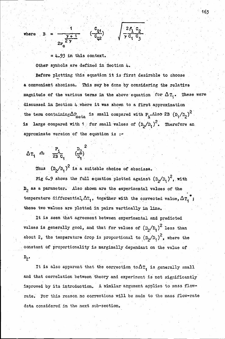
where B = 1
Y+ 1
2rc2 Y
= 4.93 in this context.
Other symbols are defined in Section 4.
Before plotting this equation it is first desirable to choose
163
a convenient abscissa. This may be done by considering the relative
magnitude of the various terms in the above equation for tl T1• These were
discussed in Section 4 where it was shown to a f'irst approximation
. )2 the term containingtlPmeta is small compared with pi.Also 2B (D/D2 2 is large compared with 1 .·· f'or small values o:r (D~D1 ) • Therefore an
approximate version c:r the equation is :-
Thus (D~D1 )2 is a suitable choice of abscissa.
Fig 6.9 shows the f'ull equation plotted against (D:(n1 )2, with
D2 as a parameter. Also shown are the experimental values of the
temperature diff'erentiaJ, tlT1, tog~ther with the c_orrected value, tlT~ *;
these two values are plotted in pairs vertically in line.
It is seen that agreement between experimental and predicted
values is generally good, and that :ror values
about 2, the temperature drop is proportional
constant of proportionality is marginally dependant on the value of
It is also apparent that the correction totlT1 is generally small
and that correlation between theory and experiment is not sigpificantly
improved by its introduction. A similar argument applies to mass flow-
rate. For this reason no corrections will be made to the mass f'low-rate
data considered in the next sub-section.
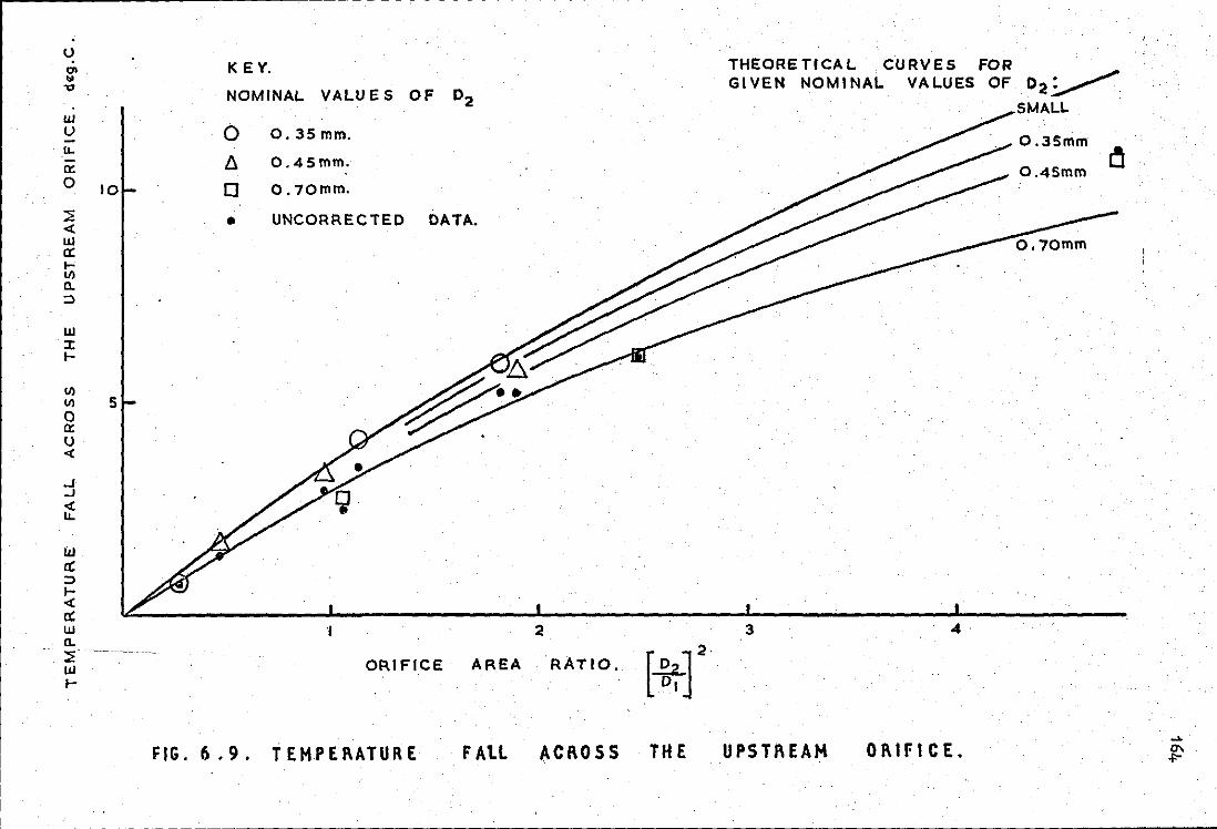
.-----------------------------------~---------------------------------------------------------------- -
u "' .. ...,
KEY.
NOMINAL. VAL.U E S OF 02
THEORETICAL. CURVES FOR . GIVEN NOMINAL. VAL.UES OF 02~
SMAL.L UJ u - 0 0. 35 mm. lL.
er: fj, 0.45mm. 0 10 0 0. 70mm.
::;; < • UNCORRECTED DATA • UJ a: 1-ll)
a. ::::l
UJ :t 1-
ll) ll) 5 0 a: u <(
..J
..J
< IJ..
UJ a: ::::l 1-< a: UJ ., 2 3 4 a. ::;; UJ OR. I FICE AR.EA R.ATIO. 1-
FIG. 6.9. TEMPERATURE FAtL ~CROSS THE UPSTREAM 01\IFICE.
165
6.4 EXperimental verification of the ex~ression for the mass
flow-rate through a two-orifice nozzle assembly.
In the previous sub-section experimental support for the
theoretical. expression for the temperature drop across'the first orifice
6 T1
was given_: This expression is required to predict the mass flow
rate and exit velocity of the spray in terms of fundamental data.
In this sub-section predicted mass flow-rates will be compared with
theory while the exit velocity of the spray will be considered in a later
sub-section, 6.6.
A fundamental express:lonfor the mass flow-rate may be obtained
by considering flow through the first (upstream) orifice. The equation
for this flow was shown in sub-section 6.2.1. to be :-
•
In that sub-section a value of O. 78 was derived for CQ1 •
Now if' the propellant, both above the first orifice and in the
expansion chamber is saturated, then :-
pi - Pe = C3 6 T1 ,
as discussed previously.
Therefore il = o. 78 (TT/4) n/ I 2fl c3 6 T1
where 6 T1. is given by eqllation 4.2.31.
If metastability is significant then the equation becomes :-
. Here6Pmetamay be obtained from the empirical equation, 4.2.27.
--------------------~--------------------------------------~----- ----
This last equation may be further developed by substituting the
expression (equation 4.2.31) for LlT1
Therefore
1 where again B = '
. = 4.93
166
Other symbols are as defined in rS:::e:.:::c.::tl.:::.' o::::n~4!:!'-----....,----------;;--D 2 D 2
Therefore:-
M = o. 78 (lT/4) J 2 r1 D 2
1
+ B(D1) ) + ~ p t (1 + 2B(D1) ) 2
me a 2
D 2 1
1 .. 2B(D) 2
= o. 78 (rr/4) J 2 r1
It is
cancelled.
(2B +
seen that the two tenns containing ~p . have partly me-ea
Further for most nozzles the term 6Pmeta B(D1 /D2)2 is small
compared with P .• _Therefore, ignoring,initially, the metastability term, the mass ~ .
flow-rate M may be plottea. linearly against n1 n2 with D/D1 as
parameter.
Fig. 6.10 shows the above ey_uation plotted, with the parameter
n2;n2 = 0,1 ana. 2, thus covering the range of orifice diameter ra tics
T· u .. .. 0>
""' Ill 1-4: 0:
;!::
.0 ..J u..
11) 11)
4: ~
-3 3X 10
2
·10
THEORIO: TICAL
THREE. Gl VE N
·20
CURVES
VALUES
·30
PRODUCT OF ORIFICE DIAMETERS 01
02
. m2
FIG.6.10. MASS FLOW 1\AT E THROUGH A TWO-ORIFICE
0 I 2
·40
KEY
NOMINAL VALUES OF D2/D1 0 SMALL
0
<> 2 I
---~- DENOTES METASTABILITY CORRECTION.
N 0 ZZL E. .... "' -.J
used in this work. Experimental dat~ are also plotted. In this case,
however, for reasons given in the previous sub-section, no correction
was made for sub-cooling or a non-standard initial temperature. For
four of the nozzles the assumption of negligible metastability was not
valid and a correction to the simplified equation was made; this is
shown as a dashed line related to _the relevant data point.
168
It is apparent-from Fig. 6.10 that generally, the linear relationship
between mass flow-rate (M) and the product of the diameters of the two
orifices of t~e nozzle assembly (n1n2 ) is borne out by the data.
Further the predicted trend of a reducing mass flow-rate with increasing
orifice diameter ratio n2/D2 is also supported. However, it is seen that
the slope of the theoretical prediction is slightly lower than required
by the data when the ratio D2/D1is 0 or 1; an increase of slope by 7% would produce a better correlation. This would require a discharge
coefficient of 0.84, instead of the 0.78 determined in sub~section 6.2.1.
When the ratio n2/n1 is approximately 2,.however, agreement between
data and the simplified equation (in which metastability is ignored) is
good. The necessary metastability correction impairs the agreement.
However, because only two data points with Dz/D1 equal to 2 are
available, this finding should perhaps be treated with caution.
6.5 Measurement of the velocity ratio between liquid and gas·
phases at the exit of the nozzle assembly.
In the last section, it was shown that mass flow-rate through a
two-orifice nozzle assembly could be adequately predicted in terms of
fundamental data and an empirical expression for the metastability of
'of the propellant in the expansion chamber. The mass flow-rate and
the exit velocity have been shown to be the two main parameters required
to describe velocity profiles within a spray. Having shown that mass
flow-rate can be adequately predicted it is then necessary to show that
exit velocity can also be adequately predicted. However before the
exit velocity is considered, it is appropriate to verify an important
assumption made in the theoretical development in Section 4. This
169
is that during the passage of two'-phase propellant through the downstream
orifice, the ratio of the velocity of .the liquid propellant to that of
its vapour is unity •. If this ratio, sometimes called the "slip'' factor,
were to depart significantly from unity then the development of'
theoretical expressions in. Section 4 would require significant . .
modification. Experimental evidenoe is now presented in support of
this assumption.
The velocity ratio between phases was determined by analysing
double-flash photographs taken of the spray at the nozzle housing exit. The
analysis consisted of the measurement of the displacement and diameters
of pairs of particles. The velocity of the gaseous phase was obtained
by measurement of the velocity of very small particles.
For this method to be effective therefore! it was desirable. to obtain
the displacement of particles below about 10~m in diameter. In
order that pairs of particles of this diameter could be identified against
a background crowded with other particles, a flash interval to about 2 or
3 microsecondswas necessary. However, with such a small time interval
: '
I I ' !
I
I ' !
.170
and because of· the limitations of the resolution of the oscilloscope and
interval timer, absolute velocity measurements were rather inaccurate.
However velocity ratio measurements were satisfactory.
A total of 16 double flash photographs were analysed. From each
photograph, the distance between all identifiable pairs of particles was
measured, together with the particle diameter. The data were classified
according to particle size. The mean displacement for each class of
particle diameter vras then calculated; this vras a spatial mean displacement.
From these mem values the overall mean over a number of photographs -
or the temporal mean, was calculated for each diameter range for a given
nozzle. Also calculated were the standard deviation and standard error
of the mean. Thus, three statistical indices were determined for each
nozzle for a nominally constant flash· interval. Statistical indices
were calculatecl for .the temporal data rather than the ·s·patial data because
the former, being the mean of data from several photographs were considered
the more reliable.
The results are shown in Table 6.1, overleaf. The displacement
between the particles is shown as a "nominal" velocity, that is, displacement
divided by nominal flash interval.· It is seen that there is negligible
.variation in particle velocity with increasing particle size, up to a
particle diameter of about 50 pm, the maximum observed.
.-------------------------------------------------------~----------------------------------------~----
NOZZLE
320 X 350
320 X 350
320 X 450
450 X 450 .
680 X 700
TABLE 6.1
DISTANCE FROM NUMBER OF NOZZLE EXIT PHOTOGRAPH!
NO!.!INAL FLASH NID!BER OF INTERVAL PARTICLES
-5
0 mm 3 -2,4 jlSBC 23
5 nun 4 24 2.4 pseo 40 2
1
0 mm 4 3.5 18 -pseo
.
5 mm 4 3.5 52 I -pseo .
0 mm 1 2.5 J!S9C 15 -
.. MEAN "NOMINAL" VELOCITY m/sec STANDARD DEVIATION m/sec IN THE GIVEN
STANDARD ERROR OF ME!Jf m/seo PARTICLE SIZE RANGE (" m);
.
5 - 10 10 - 15 15 - 20 20- 25 25- 30 30 - 40 40- 50 50- 60
29 28 - 2 3
1 2
26 25 25 4 2 2 2. 1 1
38 - - 4.0
. 2.0
31 30.5 32 2.9 2.6 2,6 1.4 1.4 1•4
31 31 33 2.0 2.0 2.0
1.2 0.8
29 27 27 27 2 2 -1 1.5
29 27 26 27 25 3 1 1.5 .5
38 37 38 4.5 5.1 5.1 - -2.3 2.5 2.5
30. 30 2.3 2.0 -1 .1 1 .1
30 31 . 1. 6 2.0 -0.8 1.2
"' "Nominal".velooity = distance1between iiiiage pa rs nominal1flash ~nterva
DETERMINATIOlq OF VELOCITY RATIO BETWEEN LIQUID AND VAPOUR PHASES:
VARIATION OF EXIT VELOCITY WITH PARTICI&._ill]..
. '
6,6 Measurement of the exit velocity of the spray and comparison
with theory.
Having shown, in the last sub-section, that the concept of a single
exit velocity independent of particle size,· is applicable to a spray, it
is appropriate to compare experimental values of this exit velocity with
theoretical predictions. Having done this, then the two main parameters
required to describe the velocity profiles within the spray~ mass flow-
rate, and exit velocity, will have been considered.
Two expr~ssions from which the exit velocity of the spray may be
derived were given in Section 4. The first was applicable to non-
choking flow (equation 4.2.7) and gave the ·exit velocity, u , directly. 0
The second was applicable to choking flow (equation 4.2.12) and gave
172
an expression for the velocity of a pressure· pulse u through the two-phase s
propellant at the point of choking within the downstream orifice. The
exit velocity was then assumed to be equal to this pressure pulse velocity,
However it was demonstrated in Section 4 that the static pressure within
the nozzle, because of choking, was higher than ambient, and that within
a few nozzle diameters downstream the static pressure had returned to
ambient with a consequent rise in the velocity of the jet. In practice
it was possible to photograph the spray only after all,or a substantial
part of this expansion had taken .place. This was because of the maskL~g
effect of the nozzle housing. Consequently the measured jet velocity was
expected to be somewhat higher than the sonic velocity, u 8
This increase
in velocity may be determined theoretically by. comparing the initial total
momentum of the jet with that of the expanded jet~ The initial momentum
of the jet was shown to be ; assuming, in the first instance no orifice
entry losses ·-
• where M is then the mass flow-rate, ~ the downstream orifice area
173
and Pc - Pamb is the gauge critical pressure.
The momentum of the expanded jet, assuming no significant entrainment
has taken place, is:-
where un is the higher, expanded jet velocity.
Therefore
The measured exit velocity may now· be compared with u above. As . n
before a comparison with the non-choking exit velocity u0
will also be
given.
In order to determine the theoretical value for un , the value of
the sonic velocity "u " must 8
first be determined. This was given equation
4.2.12 as :-
1
y q Pc 2 _!.go_ 1 - 9. u " ( . ·) (1 + ) s q fl ' go
where the parameters were defined in Section 4.
The variables are to be determined at the point of choking.
Therefore, as before, substitutions may be conveniently made as follows:-
Pc " r p ' c e
1 1
fgc "' fge (r )Y = c1 Pe (r )Y ' c c
and q = c2 6T1
Therefore the equation becomes ·-1
1
c2
6T1
) c1P6(r
0)Y 2
(1 -,. c2 6T1 r pe ) ( c ) ( 1 + u = s c2 6T1 rl c1 p rY
e c
174
Inserting values of r1
, c1, c2
r0
and y determined previously then:-
1
= 10.9 (AT1 )"2 (1 + (1 - 0.0061 AT1 )
p 3.65 x 10⁻⁶ _._e_) m/s,
is in deg. C and P in N/m2 absolute. e
AT1
The theoretical, non-choking, expression for the exit velocity may
now be considered. This was given in equation 4.2.7 as :-
1 2
(Pe - p ) q pe ,.
1 u 1 p 1 0 - q amb .j. ( Pamb = 1)
. ,. . -2 fl fge (1 - e ,.
1- 1 ,. )
- ~)] J2t p 1
- • 0061 AT1) (P - P b) + 7.67 X 10² AT1 ( 1 - ( amb) or u =
1.41 X 10³ e am · Pe 0
The two equations for the exit velocity u and u may now be compared n · o
with exit velocity data. In order that the comparison be direct, measured
values of the two variables, the temperature fall across the first orifice
A T1 and the expansion chamber pressure P e , w.ere inserted into 'the·
equations rather than the values obtained from theoretical predictions.
However, it may be shown that the difference between the theoretical curve
derived from fundamental data and that derived from empirical data, for
each of the two-expressions for the exit velocity vlill be small. This is
because the methods of predicting the two variables, AT1 and Pe (indirectly),
have been shom1 to be satisfactory.
The values of u and u are compared with measured exit velocity n o
data in Table 6.2, overleaf. It is seen from this Table that the data
were obtained from two sources, from spray velocity profile measurements
to be discussed in sub-section 6.9 and also from tha "slip" factor velocity
measurements given in the previous sub-section. As previously stated these
latter measurements gave accurate values for the velocity ratios, the
parameter then require~ but inaccurate values for absolute velocity. The
.!. 2
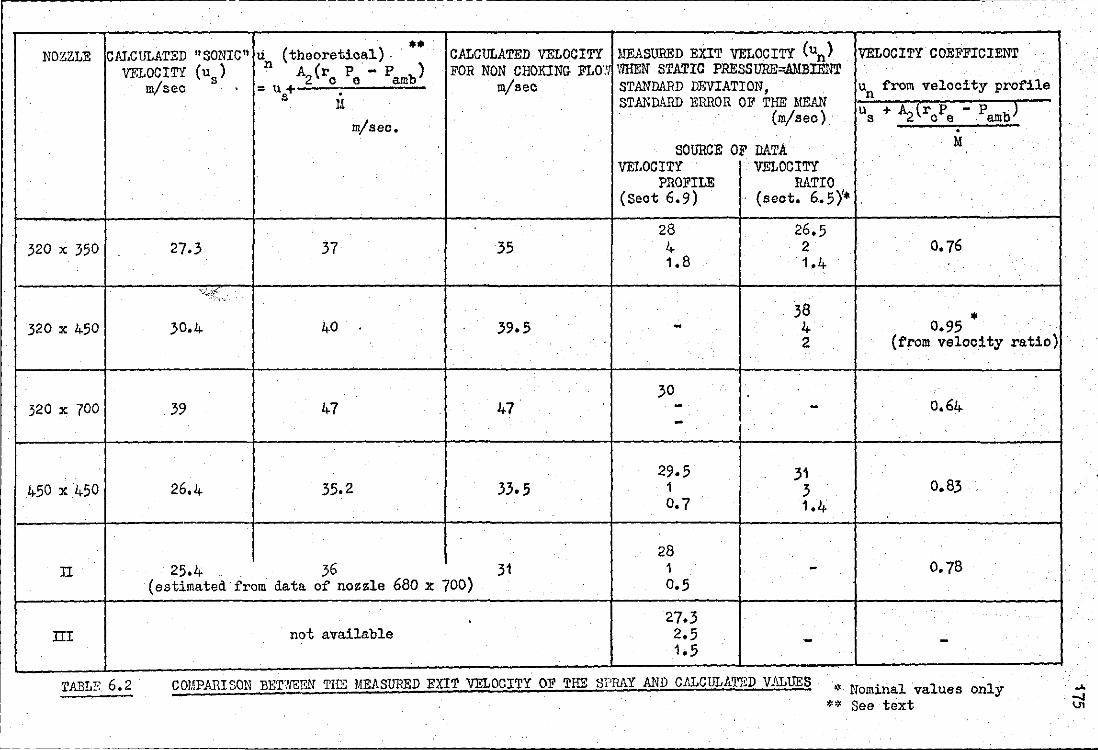
r-------------------------------------------~-------------------------------------------------------------
ti (theoretical). •• MEASURED EXIT VELOCITY (un) NOZZLE CAJ,CULATED "SONIC" CALCULATED VELOCITY VELOCITY COEFFICIENT VELOCITY (us)
n . ) · A (r P - p FOR NON CHOKING FLo·; WHEN STATIC PRESSURE=AMBIENT 2 c a amb m/sec un from velocity profile m/sec =u+ . STANDARD DEVIATION,
s 11 STANDARD ERROR OF THE MEAN
m/ sec, (m/sec) us +~(roPe - pambJ .
SOURCE OF DATA · M
VEWCITY VELOCITY PROFILE RATIO
(Seat 6.9) (sect, 6 .• 5 )'•
28 26.5 320 X 350 27.3 37 35 4 2 0.76
1,8 1,4 ..
'"~/:,.
38 • 320 X 450 30.4 40 39.5 - 4 0.95 2 (from velocity ratio)
30 320 X 700 39 47 47 - - 0.64 - .
. 29.5 31 450 X 450 26.4 35.2 33.5 1 3 0.83
0.7 1.4
28 IT 25.4 36 31 1 - 0.78
(estimated from data of nozzle 680 x 700) o.s .
27.3 III not available 2.5 - -1.5
TABLE. 6,2 COMPARISON BET7/EEN THE MEASURED EXIT VELOCITY OF THE SPRAY AND CllLCULATllD VALUES * Nominal values only ** See text
176
eiTOr is estimated to be· of the order of 2<J%, Da. ta from the velocity
profile measurements were of adequate accuracy but the number of velocity
profiles measured was limited to five. It is because only a small number
of such measurements were available that "slip" factor data, which would
otherwise have been rejected because of its inaccuracy, were included,
From Tabl-e 6.2 it, is seen that the velocity coefficients, each given
by the ratio of the measured exit velocity, un ,(from velocity profile
data) to the theoretical value of un , are within the range 0.64 to 0,83.
These values are comparable with the valu~ of 0,83 for the discharge .
coefficient of those short tubes given in AppendiX 3 for air flow, and with
_0,78 given in sub-section 6,2,2 for two-phase flow. As the flow regime
through a short tube is that of full tube flow, then the velocity coefficient
would be expected to be equal to the discharge coefficient. That such an
agreement, albeit only approximate, is obtained is taken as further support
for the theoretical description of two-phase flow through the downstream
orifice.
It is useful to compare the value of the exit velocity for non-
choking flow, u0
with the sonic velocity,
made in Fig. 6,11 where equations 4.2.7, giving
•
u 0
This comparison is
and 4.2.12 giving
are plotted against downstream to upstream orifice diameter ratio D2/D1
with n2
as parameter. The equations were plotted as previously
described, from empirical values of LlT1 and Pe for each nozzle.
However for those areas where no nozzle data were available, and where
interpolation was not possible, the theory was used to extrapolate the
curve from an adjacent data point. such situations are d~noted by plain
points as shown. The two equations may now be compared, It is seen that
over the range of orifice di~~eter ratios tested, from about 0,5 to about
2, the two equations predict velocities within about 20% of each other,
with the sonic velocity the lower as would be expected, Further, over this
range, the sonic velocity varies over the rather narrow range from
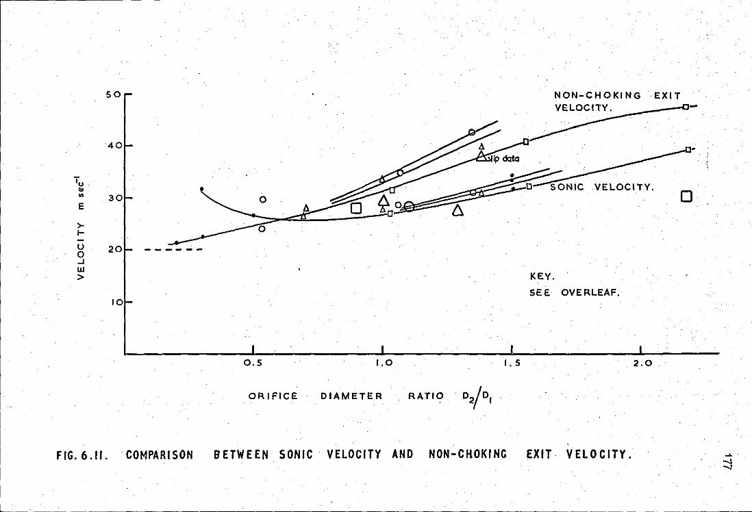
50 NON-CHOKING EXIT VELOC I TY'f .. ._ ___ --tl
40
Tu .. 0 .. 30
E
>-1--u 20 ------0 ..J w > KEY.
SEE OVERLEAF. 10
0.5 1.0 I. 5 2.0.
ORIFICE DIAMETER
FIG. 6.11. COMPARISON BETWEEN SONIC VELOCITY AND NON-CHOKING EXIT VELOCITY.
L_· ______ _ --------~-----------------------·----- - -
.... -..1 -..1
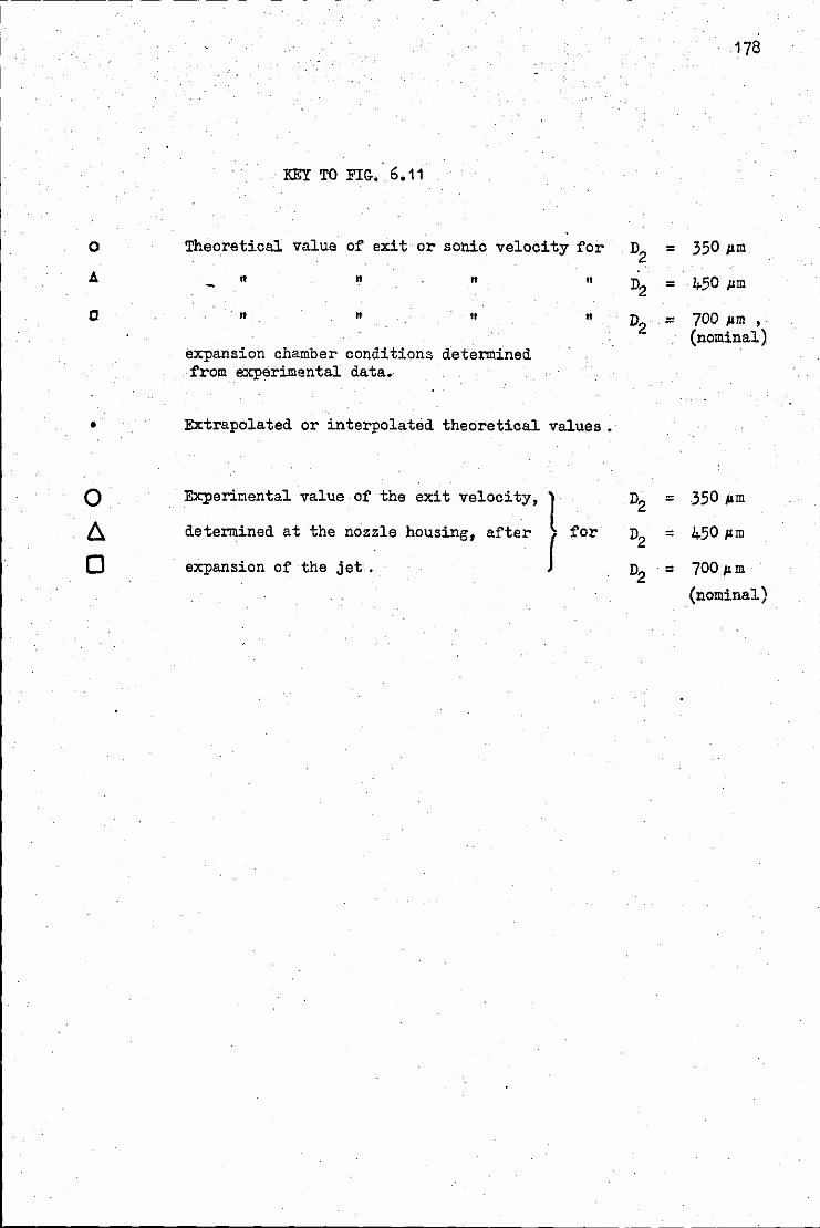
178
KEY TO FIG-. 6.11
0 Theoretical value of exit or sonic velocity for D2 = 350 11m
A n n n " D2 = 4-50 .um
c " " 11 11 D2 = 700 .um , (nominal)
expansion chamber conditions determined from experimental data.
• Extrapolated or interpolated theoretical values •
0 Experimental value of the exit velocity, l D2 = 350 11m
D. determined at the nozzle housing, after for D2 = 4-50 11m
I 0 expansion of the jet • D2 = 700 11m
(nominal)
L---------------------------------------------------------··--·-
-------------------------------------------------------------------------- - - -
179
2,5 m/sec. to 40 m/sec. while the non-choking velocity varies from 25m/sec to 4"PlJ/sec.
Beyond this range of orifice diameter ratios, for values of n2/n1 less than
0.5, the conventional,_ non mass limiting , equation predicts the lower velocity.
The reason for this reversal, as described previously,_ is that at these
low values of. orifice diameter ratio, D/D1, the fraction of' propellant
. evaporated is very low, the mean density of the propellant approaches that
of the liquid, and the expansion chamber pressure is no longer capable of'
sustaining the high "sonic" discharge velocity. Thus for a value of n2/D1
less than 0,5 the conventional equation' mu~:t be used. The limiting
velocity as n2/n
1 approaches 0 is that of' the discharge of' liquid
propellant of' density 1.4 kg/~ sustained by a pressure differential
equal. to :-
(the initial pressure, 390 kN/m2 - ambient pressure).
This discharge velocity is 20 m/sec,
It is also apparent that the two curves -will cross not only at low
values of n2/n1, but also at a value of nztn1 greater than 2. This is because,
for high levels of n2/D1, the temperature fall, and hence the pressure fall,
across the first orifice will be high; consequently the expansion chamber
pressure will be low, Agairi, therefore, the expansion chamber pressure
would not oe able to sustain the high sonic discharge velocity,
· Values of the measured exit velocity, u are also plotted in Fig, 6,11, n
Comparisons between measured and theoretical values were discussed previously.
6.7 Experimental determination of the transverse profile. of
longitudinal velocity within the. spray.
The main parameters in the equation describing the longitudinal
profiles of velocity within a spray have been discussed. These were
the mass flow-rate and the exit velocity. Before the applicability
of the velocity profile equation can be tested directly,however.two
further assumptions made in Section 4 will be considered, and the
measurement of a minor empirical parameter will be described. The
first of the two assumptions is that the transverse profile of
longitudinal velocity of the gaseous componant of the spray was
Gaussian and the second is that the divergence angle of the spray
was approximately equal to that. of an air jet; the minor empirical
factor is the position of the apparent origin of the spray. The
first assumption is considered in this sub-section, the second, together
with the position of the spray origin, is considered in the next sub
section.
The !iSSumption of a Gaussian transverse profile of longitudinal
gaseous velocity scarcely needs experimental verification as there are
many reports. in the literature ( 49,.21,34 for example) which show that
~he transverse distributions of velocity within single phase jets;
180
liquid sprays and dust-laden gas jets are Gaussian, However, experimental
determination of this transverse profile not only verifies the
assumption but also enables an assessment to be made of the divergence
angle of the jet.
Because a substantial amount of evidence already exists to vindicate
the first assumption only one such profile was measured. This VIas for
a distance of 80mm. from nozzle m; the profile is ·shown in Fig. 6.12.
It was developed from measurements of the diameter and velocity of
aerosol particles, as described later. Also plotted in Fig. 6,12 is
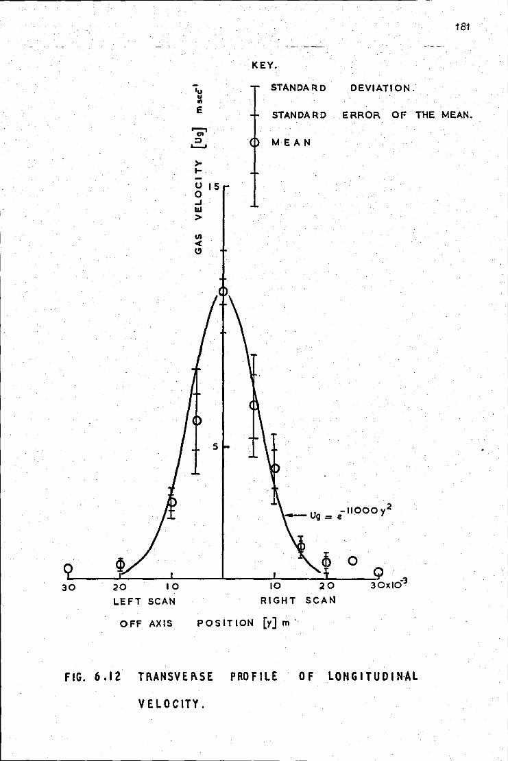
'u " ..
KEY.
STANDARD DEVIATION.
181
e STANDARD ERROR OF THE MEAN.
30 20 10
LEFT SCAN
OFF AXIS
> 1--u 15 0 ...1 Ill >
5
MEAN
10 20
RIGHT SCAN
POSITION (y)m'
F I G. 6 • I 2 T I\ AN S V E 1\ 5 E P RO F I LE 0 F L 0 H G I T U D I N·A L
VELOCITY.
I
' '
I
I
. I
I
182
the Gaussian function:~
= 11 e-11000/ m/sec. ,
where u is the velocity of the gaseous compona.~t and y(in metre) g
is the off-rucis distance.
It is seen that agreement between the data and this function is
-reasonably good except at distances from the axis of greater than about
20mm. Beyond this distance the. spray velocity is of the order of 0.5 m/sec.
while the Gaussian distribution function predicts 0.14 m/sec. and 0.5 x 10-~/sec
at off-axis distances of 20mm and 30mm respectively. The reason for this
is presumably that the measured velocity of about 0.5 m/sec., which is
vertically dovmwards, is the sedimentation velocity of the aerosol cloud
at the periphery of the spray. A velocity of this magnitude is to be
expected for the sedimentation of. such a cloud. This is because the
te:nninal velocity of 25pm particles, for example, is about 0.25 m/sec
and a cloud of such particles would fall at a higher veloc.ity depending
on its concentration •. Thus a cloud containing a range of particle sizes
.up to about 40pm,as is the case with these sprays, may well fall a~
0.5 m/sec. with the larger particles falling considerably faster. This
relative distribution of velocities is found to be the case as is demonstrated
in the latter part of this sub-section.
The data points in Fig 6.12 appear to be distributed slightly
asymmetrically about the ordinate. This is probably due to an error in
·the setting of the nozzle re.lative to the camera. As explained in Section
5, this alignment was achieved by forcing water through the nozzle and
then by focusing on the water jet. An off-set of about 2mm, which is
sufficient to cause the assymetry, would be difficult to eliminate at
a distance of 80mm. Also it is possible that the water jet and spray do not
have a cow~on axis.
The development of Fig.6.12 may now be considered. Each data point,
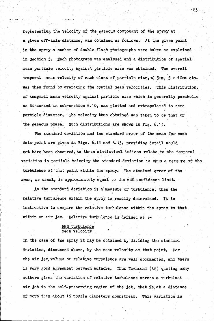
183
representing the velocity of the gaseous componant of the spray at
a given off-axis distance, was obtained as follows. At the given point
in the spray a number of double flash photographs were taken as explained
in Section 5. Each photograph was analysed and a distribution of spatial
mean particle velocity against particle size was obtained. The overall
temporal mean velocity of each class of particle siz.e, < 5!'m, 5 - 10,.m etc.
was then found by averaging the spatial mean velocities, This distribution,
of temporal mean velocity against particle size which is generally parabolic
as discussed in sub-section 6,10, was plotted and extrapolated to zero
particle diameter, The velocity thus obtained was taken to be that of
the gaseous phase, Such distributions are shown in Fig. 6,13.
The standard deviation and the standard error of the mean for each
data point are given in Figs. 6.12 and 6.13, providing detail would
not.have been obscured. As these statistical indices relate to the temporal
variation in particle velocity the standard deviation is thus a measure of the
turbulence at that point within the spray, The standard e=or of the
mean, as usual, is approximately equal to the 68% confidence limit.
As the standard deviation is a measure of turbulence, then the
relative turQulence within the spray is readily determined. It is
instructive to compare the relative turbulence within the spray to that
within an air jet. Relative turbulence is defined as :-
RMS turbulence mean velocity •
In the case of the spray it may be obtained .by dividing the standard
deviation, discussed above, by the mean velocity at that point. For
the air je~values of relative turbulence are well documented, and there
is very good agreement between authors. Thus Townsend (66) quoting many
authors gives the variation of relative turbulence across a turbulant
air jet in the self-preserving region of the jet, that is, at a distance
of more than about 15 nozzle diameters downstream. This variation is
_j
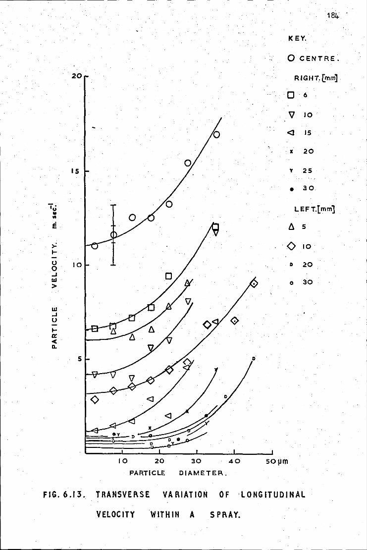
184
KEY.
0 CENTRE.
20 RIGHT.(mm]
0 6
V 10
<] 15
·X 20
IS y 25
• 30
"j· LEFT.[ mm] u .. .. e 6 5
>= 0 10 t-
u 10 D 20 0 ...1 111
0 30 >
111 ...1 u t-er < D.
5
10 20 30 40 SO!Jm PARTICLE DIAMETER..
FIG. 6.13. TRANSVERSE VARIATION OF ·LONGITUDINAL
VELOCITY WITHIN A SPRAY.
185
shown in Fig 6.14, where the relative turbulence is plotted as a function
of ratio of local mean velocity to axial velocity. Also plotted for
comparison are the values of relative turbulence, as defined above, for
the spray. It is seen that in the central region of the jet :-
0.5 ~(ratio of local mean to axial velocity) ~. 1.0,
the relative turbulence of the spray is very close to that of the air
jet. At the outer regions of the spray, agreement is not so good.
It is concluded therefore that, on the basis of data from this one
nozzle, the transverse distribution of longitudinal velocity is Gaussian,
in the developed region of the spray, and that the turbulence properties
of the spray are similar to those of an air jet.
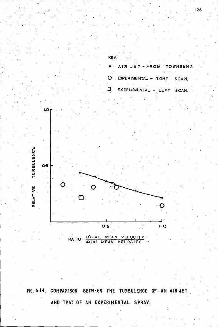
w u z w ..J ::I m a: ::I .....
w > ~ ..J w a:
J,()
0·5
0
KEY.
• AIRJET-FROM TOWNSEND,
0 EXPERIMENTAL- RIGHT SCAN.
0 EXPERIMENTAL - LEFT SCAN.
0•5
RATIO:LOCAL MEAN VELOCITY AXIAL MEAN VELOCITY
0
1·0
186
FIG. 6.14. COMPARISON BETWEEN THE TURBULENCE OF. AN AIR JET
AND THAT OF AN EXPERIMENTAL SPRAY.
-- -~_j
6,8 Measurement of the divergence angle of the spray, and the
determination of the position of its apparent origin.
Two assumptions made in the theoretical development in Section 4,
have now been verified. A third, that the divergence angle of the spray
was approximately equal to that of an air jet, may now be considered,
A related parameter, the position of the apparent origin of the spray
will also be considered.
6, 8,1 Measurement of the divergence angle of the spray,
It was shown in Section 2 that the developed spray consisted mainly
of entrained air, It is therefore relevant to compare experimentally-
determined spray angles with the spray angle for a circular turbulent
air jet, This angle is given by Towns end ( 66 ) , again quoting numerous
references, as 4;8° for the half-angle of air jets, determined.for the
locus of' points where the mean off-aids longitudinal velocity has fallen
187
to half the mee.n axial longitudinal velocity. This value may be converted
to the half-angle corresponding to 1/e of the axial velocity, the angle
used in Section 4, by assuming a Gaussian lateral distribution for
longitudinal velocity; thus, this 1/e-velocity half-angle of' an air jet
. 80 is 5, ,
The effect of loading the air jet with an aerosol may be considered,
Laats ( 34), for example, has shown that loading an air jet with ash
reduced the spread of the jet; this consequently resulted in a reduced
longitudinal attenuation of the jet. It was found however that a mass
flow-rate of ash equal to the initial mass flow-rate of' the air reduced
the half-velocity divergence half-angle by only a very small angle. This
was from 4.85° (a 1/e-velocity angle of 5.85°) to 4.3° (a 1/e-velocity
angle of 5.2°). This applied at a distance do11nstream of 15 to 20
nozzle diameters. At this downstream distance the mean ratio, by mass,
of ash to air is estimated to be approximately 0.2. This situation can
188
now be related to the present case. This same ratio, by mass, of
liquid aerosol to entrained air would be obtained, for a non-evaporating
propellant at a distance of about 160m:n from the 680 x 700 nozzle assembly
and about 80mm from the 320 x 350 nozzle assembly. Further, the propellant
is evaporating and therefore the aerosol-to-gas ratio would be considerably
less than the 'Value of 0,2 quoted above. It would not seem unreasonable
to assume, therefore, that beyond a few centimetres downstream of the
nozzle, the liquid aerosol content will have negligible effect on the
divergence angle. As the vapour concentration rapidly diminishes also,
the divergence half-angle of the spray will be taken as that of an air jet,
which is 5.8° ,for the ·1/e-velocity J.ocus,beyond the first few centimetres.
Limited experimental support for this assumption may be obtained
from the data given in the previous sub-section, There, it was seen
that at a distance of 80mm from the nozzle the spray half-width,
corresponding to 1/e of the axial velocity was given implicitly by:-
-11000y2 1/e = e ,
or y = 9.5mm
The average divergence angle over the first 80mm of the spray may now
.be determined providing the position of the apparent origin of the spray
is known. With air jets this origin is downstream of the nozzle. With
the spray generators in these experiments the spray-origin appeared to be
upstream of the nozzle; this was because of.the rapid expansion ~ediately
downstream of the nozzle, as described earlier. An assessment of the
position of the apparent origin of the spray was obtained as described
in 6.8.2. The result is quoted here. For nozzle assemblies whose
orifice diameters were.approximately equal, the origin. of the spray
was estimated to be about 30mm upstream of the second orifice. For
nozzle assemblies such as nozzle IT! for which the ratio of the second
orifice diameter to that of the first was about 1.3, the corresponding
upstream distance was approximately 25mm.
The divergence half-angle, oorrespondi.ne; to the 1/e-velooity locus
is therefore given by :-
= tan-1 (9.5/(80 + 25) ) 0 =. 5.2 •
This figure is in agreement with the value given by Laats for an
ash-laden air-jet. That the two values coincide is fortuitous., This
is because of the physical differences between the developing spray and
the laden air-jet, and further because o:f the uncertainty :in the value
of the effective diameter of the spray, 9.5mm in this case, as was seen
189
in the previous sub-section, and also.because of doubt about the accuracy
o:f the origin upstream of the spray, 25mm in this case, as is demonstrated
in 6.8.21 below.
This agreement however does give limited support to the initial
assumption that, beyond a few centimetres downstream of .the nozzl~ the
effect of the aerosol and vapour content on the divergence angle of what
is essentially an air-jet may be neglected.
6,8,2 Assessment of the position of the spray origin.
A description of the assessment of the position of the spray origin
may now be given. This was obtained by takirig photographs of the flood
lit spray at a distance of about 1 metre. The position of the origin
of the spray was then determined by tracing the outline of the spray,
from the projected image, and extrapolating upstream to the apparent
origin. Because of the nebulous nature of the edge of the spray, this
method is not precise. Further it is doubtful whether the origin,
as determined by this method, is equivalent to the origin required by
the mathematical development of Section 4, this latter being the apex
of the cone which is the loci of points where the spray velocity has
fallen to 1/e of the axial value. The most satisfactory·method of
I
measuring spray-angle, therefore, would have been to have repeated the
transverse scan, described in 6.7, at many distances from the origin.
However in the absence of such data, the results of the photographic
method will be assumed to give an approximate assessment of the
position of the origin. Table 6.3 gives these results for a number
of nozzle assemblies.
NOZZLE
320 :z: 350
450 X 450
680 X 700
320 X 450
320 :z: 700
DISTANCE OF SPRAY ORIGIN UPSTREAM OF FINAL
ORIFICE (z) + STANDARD DEVIATION -(mm)
26.:!: 2
29 .:!: 1
37.:!: 6
26.:!: 4
10.:!: 1
TABLE 6.3 ESTIMATION OF THE POSITION OF THE SPRAY ORIGIN,
OBTAINED BY MACROPHOTOGRAPHY OF THE SPRAY.
"• .
It is seen that the position of the apparent origin of the spray
varies from 26mm to 37mm upstream of the nozzle for orifice pairs of
comparable diameter, while for the 320 x 700 nozzle assembly the spray
190
origin was 10~~ upstream. That this latter value should be significantly
smaller than· the others is to be expected. This is because such a
nozzle combination generates a relatively low expansion chamber pressure
(243 yJ<jm2). Thus the excess pressure in the jet at the nozzle exit,
which is responsible for the movement upstream of the spray origin,
as explained in Section 4, is ·-
= (rc243- 101) kN/m2
= 21 kN/m2 •
or, for r ::!!::: 0. 5, c
This value of 21 kN/m2 may be compared with a typical value, for
nominally twin orifice nozzles,of:-
191
(366 x r0
- 101) kN/m2 , or 82 kN/m2 , which is four times larger,
As the movement upstream of the spray origin depends on the excess
pressure in the jet, it was anticipated that the. apparent origins of
the three nominally twin-orifice nozzles would be the same, This may
possibly be the case, and the differences shown in Table 6.3 may merely
reflect a deficiency in the method of measurement. It would be expected,
for example, that as the mass flow-rate increased, with increasing nozzle
diameter, the apparent width of the spray, as recorded photographically,
would increase. This is because, at a given off-axis distance, the
concentration of spray particles would be larger for the larger mass
flow-rate. As the density of the image on the photographic film depends
among other things, on this concentration, the apparent dimensions of
the spray would appear to increase with increasing nozzle diameter,
although geometrically they had remained constant •. In the absence
of further data a mean value of 30mm will therefore be taken as the
distance upstream of the apparent origin of the spray for twin orifice
nozzles. This·distance will be considered to diminish as the ratio of
the diameters of second to first orifices rises. Thus for nozzle ni ,
for.which the position of the spray origin was required earlier, the
origin will be taken as 25mm upstream; this figure is similar to that
given in the Table fer nozzle 320 x 450 which has a similar diameter
ratio.
It is apparent that this photographic method of determination of
the distance upstream of the apparent origin of the spray is very
unsatisfactory, However as this distance may be regarded as being
merely a correction to the longitudinal dimension of the jet, i~ is
considered that such a treatment is justified.
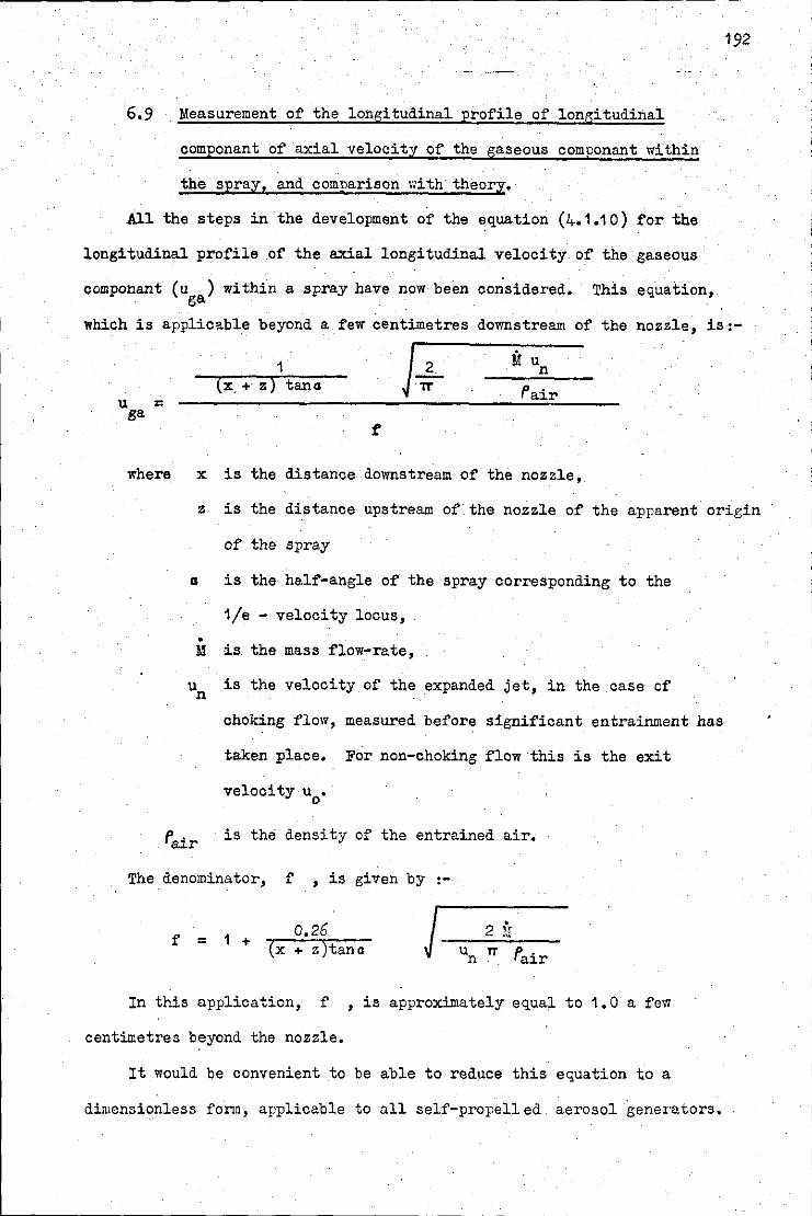
6,9 Measurement of the longitudinal profile of longitudinal
componant of axial velocity of the gaseous componant within
the spray, and comparison with theory,
All the steps. in the development of the equation (4.1.10) for the
longitudinal profile of the axial longitudinal velocity. of the gaseous
componant (u ) within a spray have now been considered, This equation, ga
192
which is applicable beyond a few centimetres downstream of the nozzle, is:-
u = ga
1 (x, + z) tan a J;
I' air
f
where x is the distance downstream of the nozzle,
z is the distance upstream of the nozzle of the apparent origin
of the spray
a is the half-angle of the spray corresponding to the
1/e - velocity locus,
• M is the mass flow-rate,
un is the velocity of the expanded jet, in the case of
choking flow, measured before significant entrainment has
taken place, For non-choking flow this is the exit
velocity u0
•
1'. is the density of the entrained air, air
The denominator, f , is given by :-
f = 1 + 0,26
(x + z)tana j _ _.::2:.-.:i~-! -un rr D , ta1r
In this application, f , is approximately equal to 1,0 a few
centimetres beyond the nozzle.
It would be convenient to be able to reduce this equation to a
dimensionless fonn, applicable to all self-propelled aerosol generators.
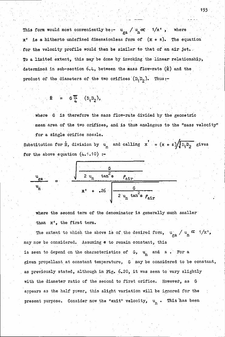
193
This form would most conveniently be:- u 1 u cc ga n 1lx' , where
x' is a hitherto undefined dimensionless form of (x + z). The equation
for the velocity profile would then be similar to that of an air jet •.
To a limited extent, this may be done by invoking the linear relationship,
determined in sub-section 6.4, between the mass flo;y-rate (M) and the
product of the diameters of the two orifices·(n1b2
). Thus:-
where G is therefore the mass flow-rate divided by the geometric
mean area of the two orifices, and is thus analogous to the "mass velocity"
for a single orifice nozzle.
Substitution fori!, division by un
for the above equation (4.1.10) :-
G
I and calling x
J 2 2
u un tan G fair ga = U· G n x' .26 + 2
2 u tanG fair n
gives
where the second term of the denominator is generally much smaller
·than x', the first term.
The extent to which the above is of the desired form,
may now be considered. Assuming G to remain constant, this
is seen to depend on the characteristics of G, u and z n
u I u a: 1lx', ga n
For a
given propellant at constant temperature, G may be considered to be constant,
as previously stated, although in Fig. 6,20, it was seen to vary slightly
with the diameter ratio of the sec.ond to first orifice, However, as G
appears as the half p~wer, this slight variation will be ie;nored for the
present purpose, Consider now the "exit'' velocity, u • n
This 'has been
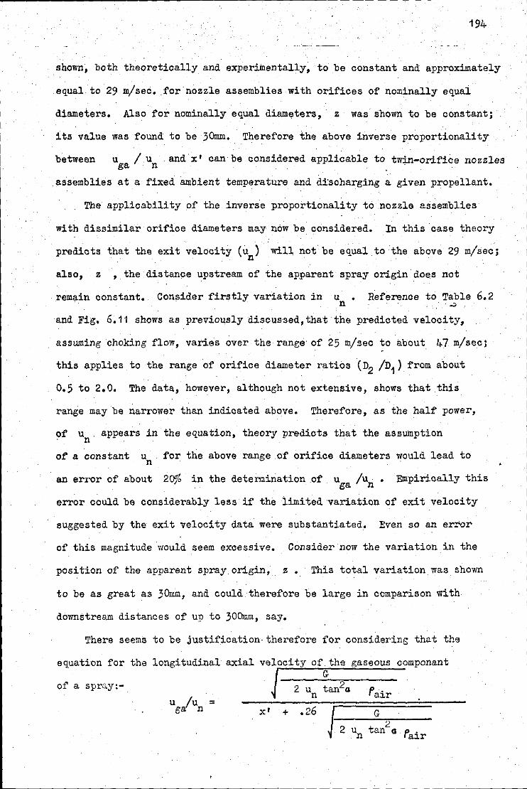
194
shown, both theoretically and experimentally, to be constant and approximately
equal to 29 m/sec. for nozzle assemblies with orifices of nominally equal
diameters. Also for nominally equal diameters, z was shown to be constant;
its value was found to be 30mm. Therefore the above inverse proportionality
be.tween u / u and x' can be considered applicable to twin-orifice nozzles P n . . . .
assemblies at a fixed ambient temperature and di'scharging a given propellant.
The applicability of the inverse proportionality to nozzle assemblies
with dissimilar orifice diameters may now be considered. In this case theory
predicts that the exit velocity (u ) will not be equal to the above 29 m/sec; . n
also, z , the distance upstream of the apparent spray origin does not
remain constant. Consider firstly variation in u n • Reference to Table 6.2
and Fig, 6.11 shows as previously discussed,that the predicted velocity,
assuming choking flow, varies over the range· of 25 m/seo to about 47 m/sec; . .
this applies to the range of orifice diameter ratios (n2 /D1) from about
0.5 to 2,0. The data, however, although not extensive, shows that this
range may be narrower than indicated above. Therefore, as the half power,
of un. appears in the equation, theory predicts that the assumption
of a constant un for the above range of orifice diameters would lead to
an error of about 2CJ% in the determination of u /u . ga n Empirically this
error could be considerably less if the limited ·variation of exit velocity
suggested by the exit velocity data were substantiated. Even so an error
of this magnitude would seem excessive. Consider now the variation in the
position of the apparent spray origin, z • This total variation was shown
to be as great as 30mm, and could therefore be large in comparison with
downstream distances of up to 300mm, say.
There seems to be justification· therefore for considering that the
equation for the longitudinal axial
of a spro.y:-
u /u = ga n
velocity of the gaseous componant
J G
2 u tan2a fair n
x• + .26
J 2
G 2
un tan a fair
L-----------------------~------ - - - - -- --
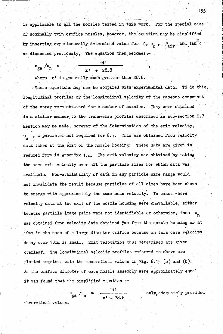
195
is applicable to all the nozzles tested in this work. For the special case
of nominally twin orifice nozzles, however, the equation may be simplified
by inserting experimentally determined value for G, un ,
as discussed previously, The equation then becomes:-
2 D and tan 11 'air
111 • x 1 + 28.8
where x' is generally much greater than 28.8.
These equations may now be compared with experimental data. To do this,
longitudinal profiles of the longitudinal velocity of the gaseous componant
of the spray were obtained for a number of nozzles. They were obtained
in a similar manner to the transverse profiles described in sub-section 6.7
Mention may be made, however of the determination of the exit velocity,
un , a parameter not required for 6.7. This was obtained from velocity
data taken at the exit of the nozzle housing• These data are given in
reduced form iri Appendix 1.4. The exit velocity was obtained by taking
the mean exit velocity over all the particle sizes for which data was
available. Non-availability of data in any particle .size range would
not invalidate the result because particles of all sizes have been shown
to emerge with approximately the same mean velocity. In cases where
velocity data at the exit of the nozzle housing were unavailable, either
because particle image pairs were not identifiable or other\vise, then un
was obtained from velocity data obtained 5mm from the nozzle housing or at
1 Omm in the case of a large .diameter orifice because in this case velocity
decay over 10mm is small. Exit velocities thus dete1mined are given
overleaf. The longitudinal velocity profiles referred to above are
plotted together with the theoretical values in ]~g. 6.15 (a) and (b).
As the orifice diameter of each nozzle assembly were approximately equal
it was found that the simplified equation ·-
theoretical val~es.
u /u = ga n 111
x' + 28.8 only,adequat~ly provided
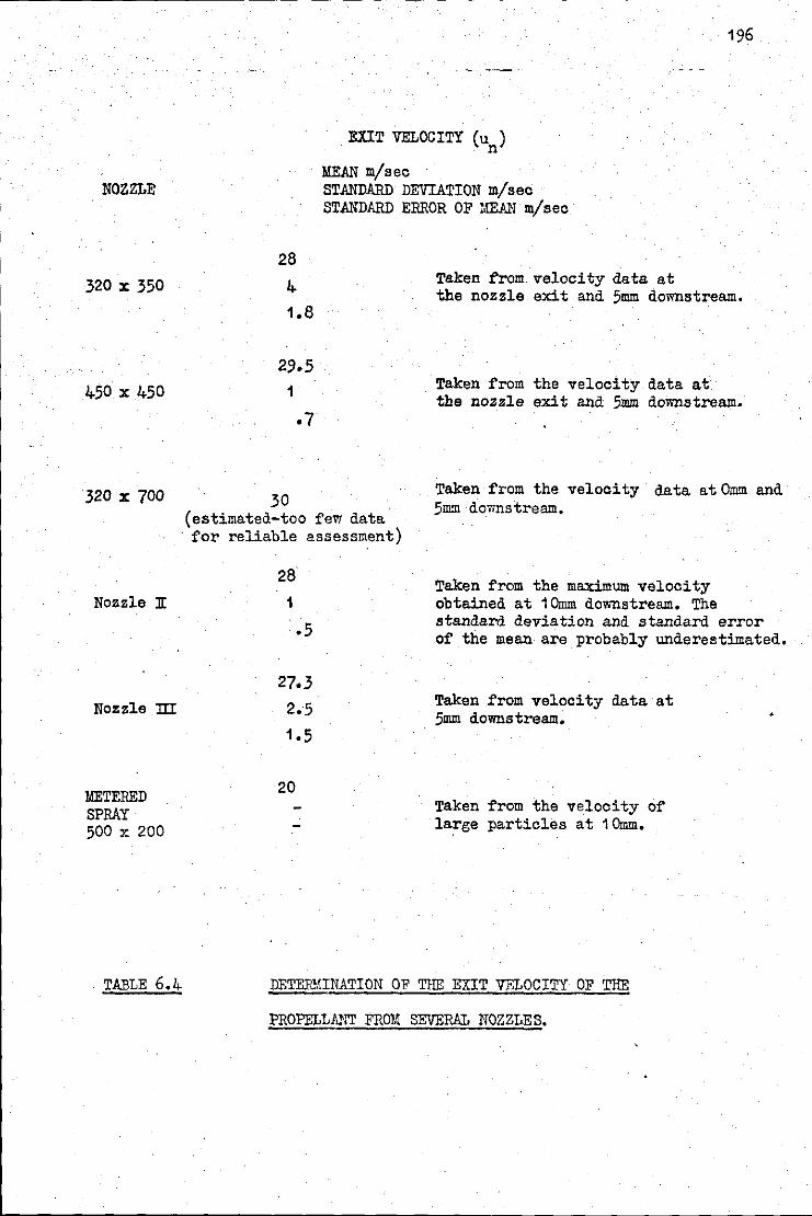
NOZZLE
320 X 350
450 X 450
28
4 1.8
29.5 1
EXIT VELOCITY (u ) n
MEAN m/sec STANDARD DEVIATION m/sec STANDARD ERROR OF l!EMI m/sec
Taken from velocity data at
196
the nozzle exit and 5mm downstream.
Taken from the velocity data at the nozzle exit and 5mm downstream.
320 X 700 30 Taken from the velocity data at Omm and 5mm downstream.
(estimated-too few data · for reliable assessment)
Nozzle :n:
Nozzle m
METERED SPRAY 500 X 200
TABLE 6.4
28
1
.5
27.3
2.5 1.5
20
Taken from the maximum velocity obtained at 1 Omm downstream. The standard deviation and standard error of the mean are probably underestimated.
Taken from velocity data at 5mm downstream.
Taken from the velocity of large particles at 1 Omm.
DETERMINATION OF THE EXIT VELOCITY OF THE
PROPELLANT FROM SEVERAL NOZZLES.
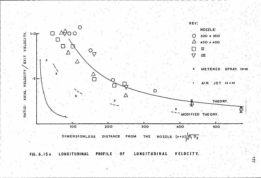
~ 1--u 0 ..J
·w > 1--X w
" >-1-u g w > ..J <(
X <(
.. 0 1-<( a:
1•0
X
·5
ti)oo 0
0 0
0 .6
!:::. \ \ \ X
' ' ..... X
lOO
0\7
!:::. 0
I< EY:
NOZZLE:
0 320 X 350
tJ 450 I( 450
0 II
\1 m
X METERED SPRAY. <z=o>
• AI Fl J E T tz " o>
x· THEORY. --X
--MODIFIED THEORY.
200 300 400 500
DIMENSIONLESS DISTANCE FROM THE NOZZLE (x+Z]/JD1 D2
FIG. 6.15 a. LONGITUDINAL PROFILE OF LONGITUDINAL VELOCITY.
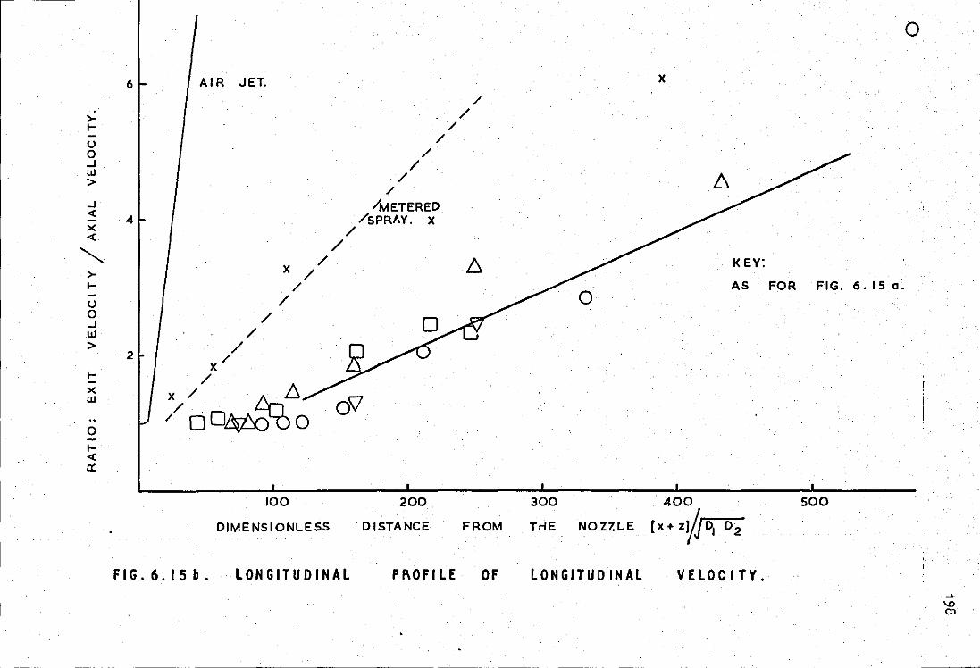
0
6 AIR JET. X
/
>- / 1- / - / u 0 / .J / llJ / >
/ .J /METERED < 4 /sPRAY. X X / <
/ ""'-· / !:-:, KEY:
>- X / 1- / AS FOR FIG. 6. IS a. - / 0 u 0 / .J llJ / > / 2
X/ 1- / X
X / f16/:-:, llJ o'V /oo~ o 0 -1-< a:
100 200 300 400 500
DIMENSIONLESS . DISTANCE FROM THE NOZZLE (x+ z0o1 02
FIG.6.15b. LONGITUDINAL Pf\OFI LE OF LONGITUD IHAL VELOCITY. ~
"' CD
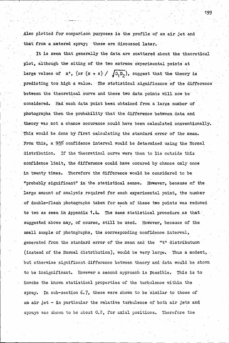
Also plotted £or comparison purposes is the pro£ile o~ an air jet and
that ~rom a metered spray; these are discussed later.
199
It is seen that generally the data are scattered about the theoretical
plot, although the siting 0~ the two extreme experimental points at
large values o~ x 1 , (or (x + z)·/ JD1D2), suggest that the thee~ is
predicting too high a value. The statistical signi~icance o~ the di~~erence·
between the theoretical curve and these two data points will now be
considered. Had. each data point been obtained ~rem a large number of
photographs then the probability that the difference between data and
theory was not a chance occuranoe .could have been calculated conventionally •
. ··This would be done by first calculating the standard error of the mean.
From this, a 95% confidence interval would be detennined using the Nonnal
distribution. If the theoretical curve were then to lie outside this
confidence limit, the difference could have occured by chance only once
in twenty times. Therefore the difference would be considered to be
"probably significant" in the statistical sense. However, because of the
large amount of analysis required for each experimental point, the number
of double-flash photographs taken for each of these two points was reduced
to two as seen in Appendix 1.4. The same statistical procedure.as that
suggested above may, of course, still be used. However, because of the
small sample of photographs, the corresponding confidence interval,
generated from the standard error of the mean and the "t" distributuon
(instead of the Normal distribution), ·would be very large. Thus a modest,
but otherwise significe.nt difference between theory and· data would be shown
to be insignificant. However a seoond approach is Possible. This is to
invoke the known statistical properties of the turbulence within the
spray. In sub-section 6.7, these were shown to be ·similar to those of
an air jet - in particular the relative turbulence o~ both air jets and
sprays v;as shown to be about 0.2, for axial positions. Therefore the
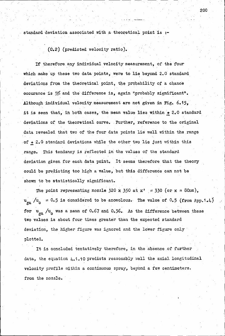
standard deviation associated with a theoretical point is :-
(0,2) (predicted velocity ratio),
If therefore any individual velocity measurement, of the four
which make up these two data points, were to li~ beyond 2.0 standard
deviations from the theoretical point, the probability of a chance
occurance is 5% and the difference is, again ·~probably significant".
Although individual velocity measurement are not given in Fig, 6.15,
200
it is seen that, in both cases, the mean value lies within ~ 2,0 standard
deviations of the theoretical curve, Further, reference to the original
data 1·evealed that two of the four data points lie well within. the range
of + 2,0 standard deviations while the other two lie just within this
range. This tendency is reflected in the values of the standard
deviation given for each data point. It seems therefore that the theory
could be predicting too high a value, but this difference can not be
shown to be statistically significant.
The point representing nozzle 320 x 350 at x' . = 330 (or x = 80mm),
uga /u0
= 0.5 is considered to be anomolous.- The value of 0,5 (from App.1.45
for u /u was a mean of 0.67 and 0.36. As the difference between these ga o . two values is about four times greater than the expected standard
deviation, the higher figure was ignored and the lower figure only
plotted,
It is concluded tentatively therefore, in the absence of further
data, the equation 4.1.1 0 predicts reasonably well the axial longitudinal
velocity profile rdthin a continuous spray, beyond a few centimeters.
from the nozzle.
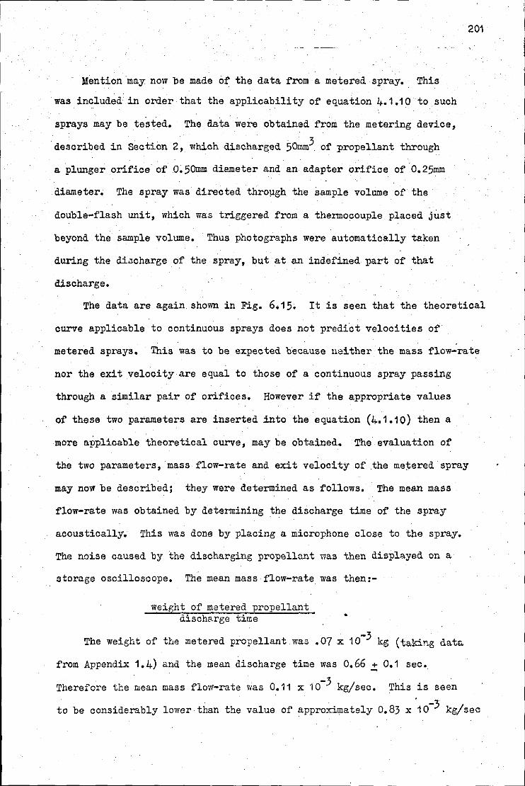
Mention may now be made of the data from a metered spray •. This
was included in order that the applicability of equation 4.1.10 to such
sprays may be tested. The data were obtained from the metering device,
described in Section 2, which discharged 50mm3 of propellant through
a. plunger orifice of 0.50mm diameter and an adapter orifice of 0.25mm
diameter. The spray was directed thro)lgh the sample volume of the
double-flash unit, which was triggered from a thermocouple placed just
beyond the sample volume. Thus photographs were automatically taken
during the di~charge of the spray, but at an indefined part of that
discharge.
201
The data are again shown in Fig. 6.15. It is seen that the theoretical
curve applicable to continuous sprays does not predict velocities of
metered sprays. This was to be expected because neither the mass flow-rate
nor the exit velocity are equal to those of a continuous spray passing
through a similar pair of orifices. However if the appropriate values
of these two parameters are inserted into the equation (4.1.10) then a
more applicable theoretical curve, may be obtained. The evaluation of
the two parameters, mass flow-rate and exit velocity of .the metered spray
may now be described; they were determined as follows. The mean mass
flow-rate was obtained by determining the discharge time of the spray
acoustically. This was done by placing a microphone close to the spray.
The noise caused by the discharging propellant was then displayed on a
storage oscilloscope. The mean mass flow-rate was then:-
weight of metered propellant discharge time •
The weight of the metered propellant was .07 x 10-3 kg (taking data
from Appendix 1.4) and the mean discharge time was 0.66 = 0.1 sec.
Therefore the mean mass flow-rate vias 0.11 x 10⁻³ kg/sec. This is seen
to be considerably lower than the value of approximately 0.83 x .10-3 kg/sec
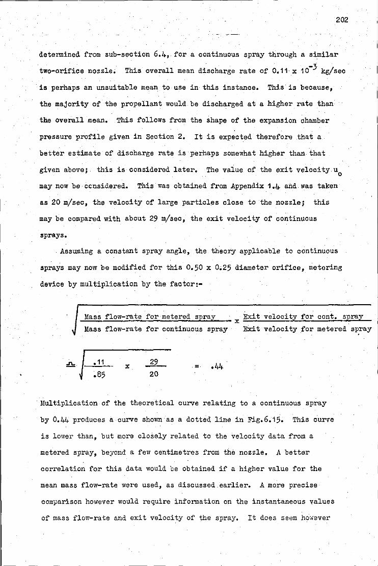
202
determined from sub-section 6.4, for a continuous spray through a similar
two-orifice nozzle; This overall mean discharge rate of 0,11·x 10-3 kg/sec
is perhaps an unsuitable mean to use in this instance. This is because,
the majority of the propellant would be discharged at a higher rate than
the overall mean. This follows from the shape of the expansion chamber
pressure prof'ile given in Section 2, It is expected theref'ore that a
better estimate of' discharge rate is perhaps somewhat higher than that
given above; this is considered later, .The value of' the exit velocity.u0
may now be ccnsidered. This was obtained f'rom Appendix 1.4 and was taken
as 20 m/sec, the velocity of' large particles close to the nozzle; this
may be compared with about 29 m/sec, the exit velocity of' continuous
sprays,
. Assuming a constant spray angle, .the theory applicable to continuous
sprays may now be modif'ied f'or this 0.50 x 0.25 diameter orif'ice, metering
device by multiplication by the f'actor:-
Mass f'low-rate for metered spray x Exit velocity f'or cont. spray
Mass f'low-rate f'or continuous spray Exit velocity f'or metered spray
.1\. J--.:.·.:..11=-• 85
x . ·44
Multiplication of' the theoretical curve relating to a continuous spray
by 0,44 produces a curve shown as a dotted line in Fig.6.15, This curve
is lower than, but more closely related to the velocity data from a
metered spray, beyond a fe1v centimetres from the nozzle, A better
correlation for this data would be obtained if a higher value for the
mean mass flow-rate were used, as discussed.earlier. A more precise
comparison however would require information on the instantaneous values
of mass flow-rate and exit velocity of the spray, It does seem ho·,;ever
203
that this theoretical approach could yield meaningful! predictions, given
expressions for the above two parameters.
It is of interest to compare the continuous and metered spray data
· with that of an air jet, also shown in Fig. 6.15. It is seen that for
given nozzle configuration, velocity decay is very rapid compared with
either of the liquid-spray decay rates, In pririciple this suggests that
a powder aerosol of lower velocity, would be more readily obtained if the.
powder is dispersed by an air or propellant vapour jet, of similar initial
velocity,rathar than by atomization of a liquid,
'§.J.2 Measurement of the variation of particle velocity within
a spray with particle size, and comparison with standard
theory,
In the last sub-section an expression for the .longitudinal velocity
profile of the gaseous componant of the spray was given, However the
pharmaceutical properties of the spray are determined by the behaviour
of its liquid or solid componant. It is therefore desirable to predict
also the velocity profiles of particles within the spray.
Figs. 6.16 (a) and (b) show longitudinal velocity profiles plotted
from the data given in Appendix 1.5. Fer each nozzle two profiles are
plotted, one for the velocity of the gaseous componant and the other
for particles whose instantaneous diameter is· 30 p. m to 35 pm.· It may be
noted that this latter profile does not represent the velocity decay of
a 30 -. 35 p.m particle because in general the particles are evaporating,
In principle two methods are available for predicting the velocity
of a particle at a given position in the spray. Firstly, using an
iterative.mathematical process, the drag on a particle could be
calculated and the total reduction in velocity along its trajectory
may be found, This method suffers the disadvantage that .the variation
in particle diameter, due to evaporation and possibly coagulation, is
generally unlmown, and: consequently large errors would appear in the
results of the calcUlation •. This method will therefore not be pursued,
A second approach is to consider the situation at a given point in
204
the spray, In this case the drag on the particle created by the relative
velocity between the particle and the spray, may be equated to the mass
of the particle multiplied by its deceleration,
Therefore:- du Drag=m.u,( P).
p p dx • • • 6.1 0.1
where m is the mass of the particle, u and (du /dx) are the p p p
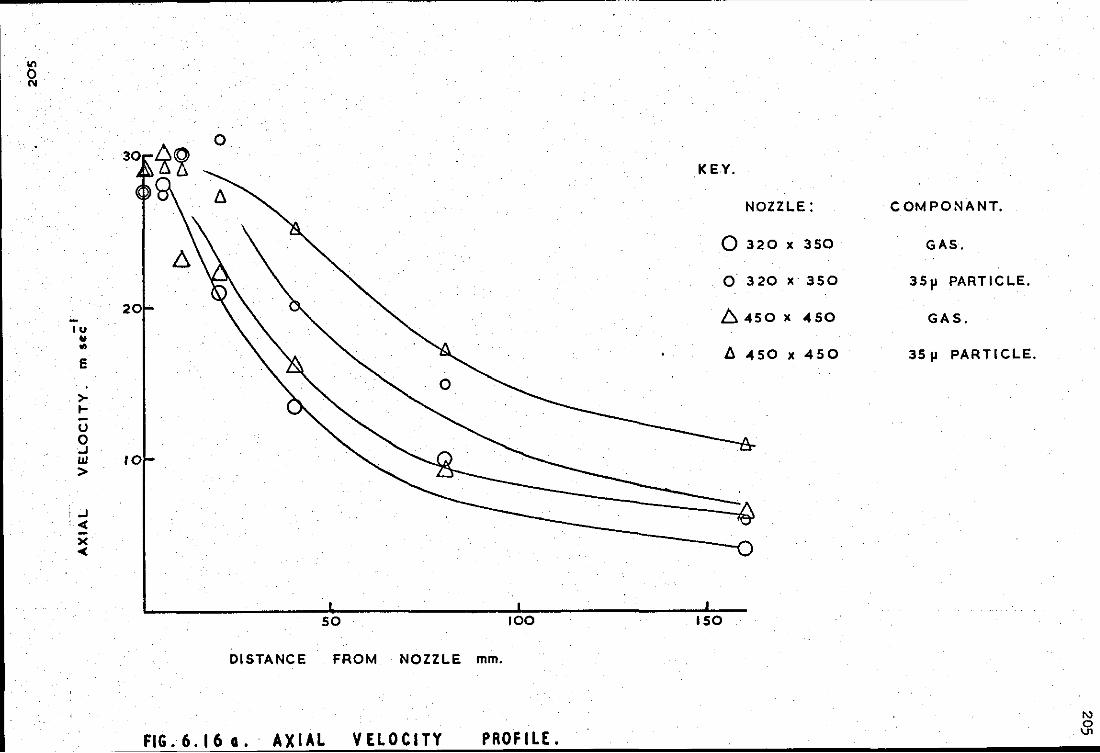
-IU .. .. E
>-1-
u 0 ..J Ul
>
·..J '<
X -<
0
so 100
DISTANCE FROM NOZZLE mm.
FIG.6.16o. AXIAL VELOCITY PROFILE.
KEY.
NOZZLE: COMPONANT.
0 320 X 3S0 GAS.
0 320 X 3S0 35f1 PARTICLE.
64SO X 4S0 GAS.
/j. 4S0 X 4S0 3Sfl PARTICLE.
ISO
30
\/0 KEY.
NOZZLE COMPONANT. 'iJ
0 \! m 370 xSOO GAS.
V m 370X 500 3Sfl PARTICLE. 20
lu 0 II 690X 700 GAS. .. .. E 0 n 690x700 35JI PARTICLE.
>- X METERED GAS; ... SOOx250 u 0
10 PARTICLE. ..J • METERED 35 fl LLJ 500x250 • >
..J < )(
·x < X
50 100 150
DISTANCE FROM NOZZLE mm.
FIG. 6.16 b. AXIAL VELOCITY PROFILE.
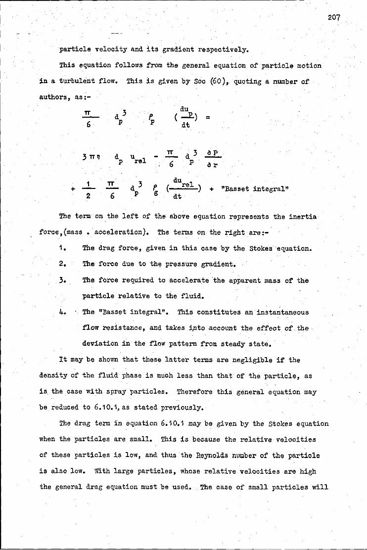
particle velocity and its gradient respectively.
This equation f'ollows f'rom the general equation of' particle motion
in a turbulent f'low. This is given by Soo (60), quoting a number of'
authors, as:-
TT
6
3 1T ~ d u -p rel
1 TT d3 +- - ~ 2 6 p
TT
du ( ......1!.) =
dt
ap - d3 6 p ar
du rel ( ) +-dt
"Basset integral"
The term on the lef't of' the above equation represents the inertia
force,(mass • acceleration). The terms on the right are:-
1. The drag f'orce, given in this case by the Stokes equation.
2. The f'orce due to the pressure gradient.
3. The f'orce required to accelerate ·the apparent mass of the
particle relative to the fluid.
4. The "Basset integral". This constitutes an instantaneous
f'low resistance, and takes i.nto account the ef'f'ect of the
deviation in the flow pattern from steady state.
It may be shown that these latter terms are negligible if the
density of the fluid phase is much less than that of the particle, as
is. the case with spray particles. Therefore this general equation may
be reduced to 6.10.1,as stated previously.
207
The drag term in equation 6.1 0.1 may be given by the stokes equation
when the particles are small. This is because the relative velocities
of these particles is low, and thus the Reynolds nvmber of the particle
is also low. With large particles, whose relative velocities are high
the general drag equation must be used. . The case of small particles will
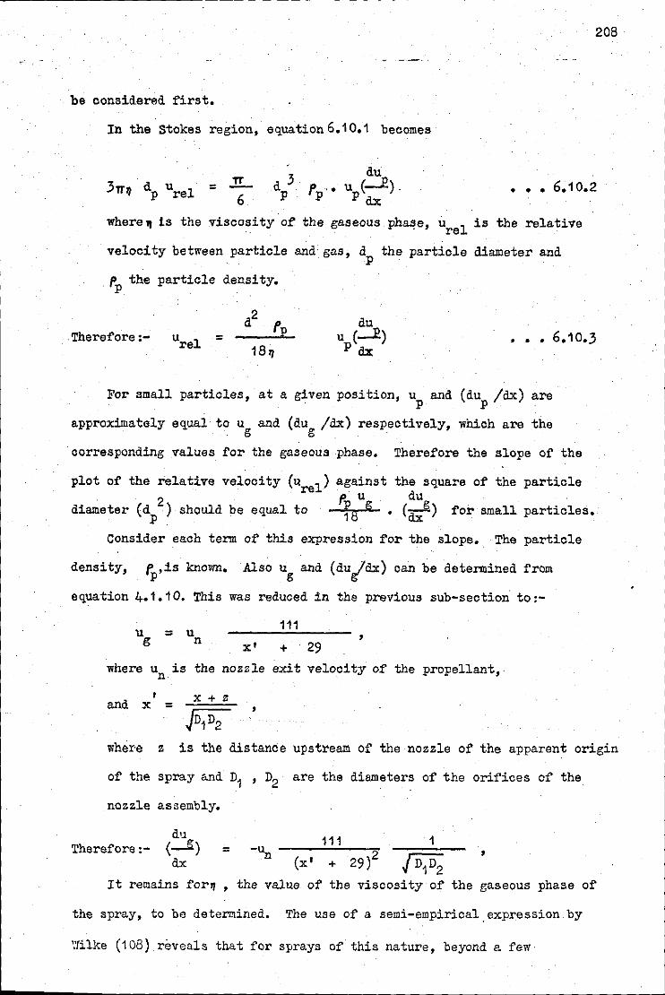
208
be considered first.
In the stokes region, equation 6.1 0.1 becomes
= .E... 6
••• 6.10.2
where~ is the viscosity of the gaseous pha~e. urel is the relative
velocity between particle and· gas; dp the particle diameter and
Pp the particle density.
.Therefore:- • •• 6.10.3 18q
For small particles, at a given position, u and (du /dx) are . p p
approximately equal to u and (du /dx) respectively, which are the g g . .
corresponding values for the gaseous phase. Therefore the slope of the
plot of the relative velocity (urel) . 2
diameter (dp ) should be equal to
against Pp u~ 18
the square of the particle du
• Ca:f) for small particles •.
Consider each term of this expression for the slope. The particle
density, fp,is known. Also ug and (dujdx) can be determined from
equation 4.1.10. This was reduced in the previous sub-section to:-
u = u g n 111
' x• + 29 where un is the nozzle exit velocity of the propellant,.
1 X + Z and x = . .. Jn1D2
'
where z is the distance upstream of the nozzle of the apparent origin
of the spray and D1 , D2 are the diameters of the orifices of the
nozzle assembly.
du Therefore:- (~)
dx =
111 -~ _ __:..:..:...____,.
(x' + 29 )2
1
' It remains for~ , the value of the viscosity of the gaseous phase of
the spray, to be determined. The use of a semi-empirical_expression by
'.'Tilke (108) reveals that for sprays of this nature, beyond e. few
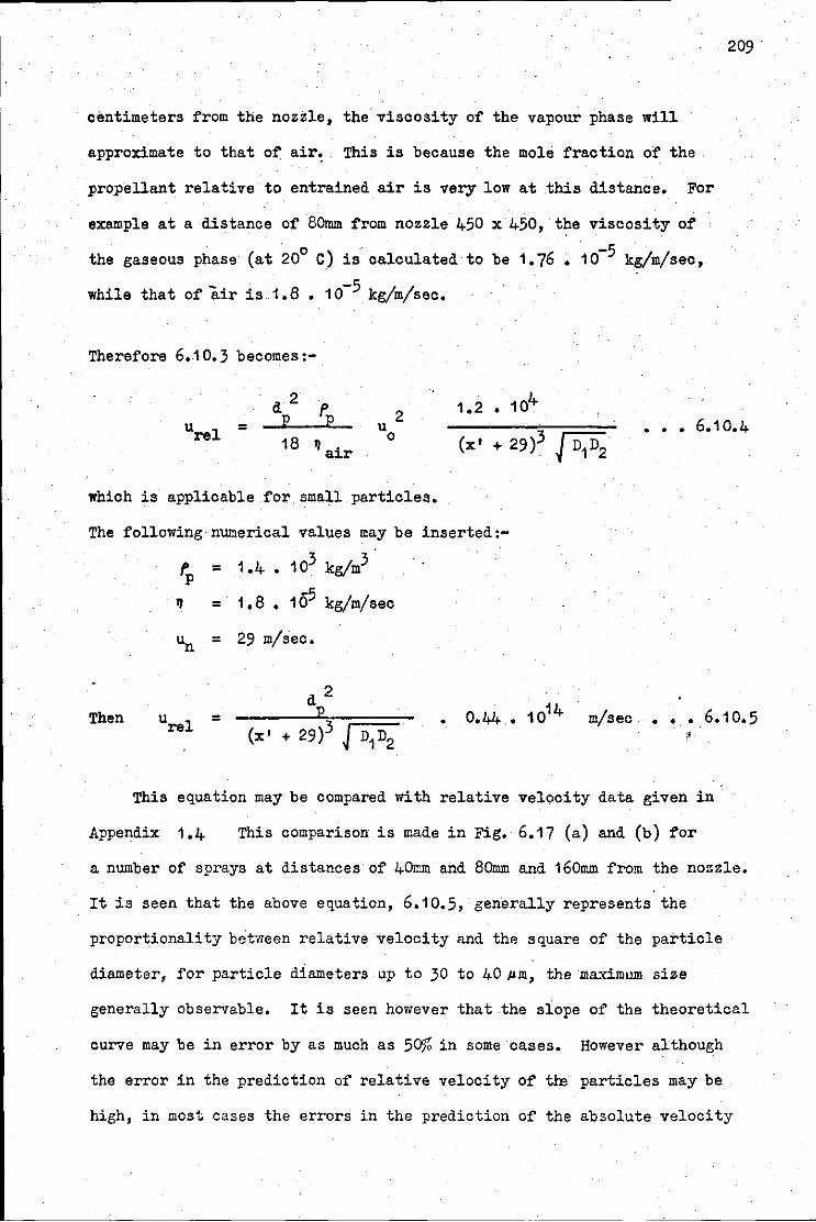
centimeters from the nozzle, the viscosity of the vapour phase will
approximate to that of air. This is because the mole fraction of the
propellant relative to entrained air is very low at .this distance. For
example at a distance of 80mm from nozzle 450 x 450, .the viscosity of
the gaseous phase (at 20° c) is. calculated to be 1. 76 • 1 o-5 kg/m/sec,
while that of air is 1,8. 10-5 kg/m/sec.
Therefore 6.10.3 becomes:-
d2
209
f'E 2 u = E u rel 0 (x 1 + 29)3 J D1D2
••• 6.10.4 18 ~air
which is applicable for small particles.
The following numerical values may be inserted:
f'p = 1,4 • 103 kgfm3
~ = 1,8 , 105 kg/m/sec
~ = 29 m/sec.
d 2 Then • m/sec ••• 6.10.5
This equation may be compared with relative vel0ci ty data given in
Appendix 1,4 This comparison is made in Fig. 6.17 (a) and (b) for
a number of sprays at distances of 40~~ and 80mm and 160mm from the nozzle.
It is seen that the above equation, 6.10.5, generally represents the
proportionality between re la ti ve velocity and the square of the particle
diameter, for particle diameters up to 30 to 40 Pm, the ma~mum size
generally observable. It is seen however that the slope of the theoretical
curve may be in error by as much as 50% in some cases. However although
the error in the prediction of relative velocity of the particles may be
high, in most cases the errors in the prediction of the absolute velocity
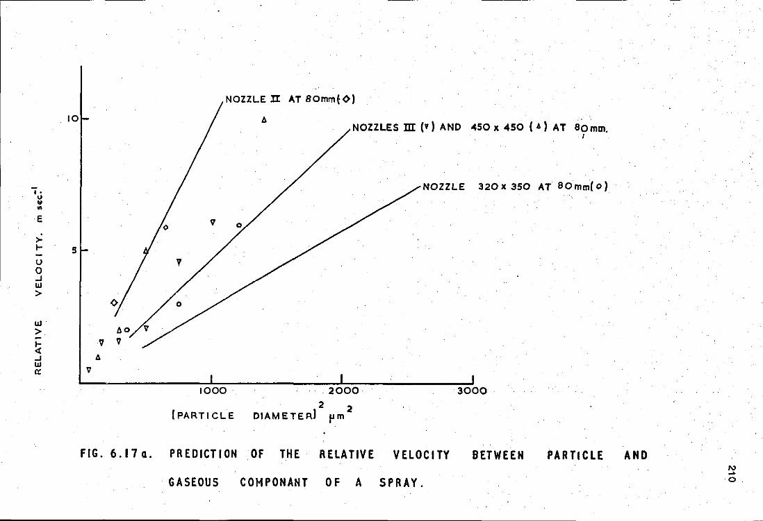
. 10
I • u .. .. E
)-... s -u 0 ...1 w >
w· > ~ ...1 w a: V
NOZZLE II AT 80mmtO)
0 /o t.o/v /
V V 6
V
1000
(PARTICLE
0
NOZZLES m (v) AND -450 x 450 ( 6) AT 80mm.
.2000
2 2 DIAMETER) pm
I
NOZZLE 320X 350 AT 80mm(o)
3000
FIG. 6.17a. PREDICTION OF THE RELATIVE VELOCITY BETWEEN PARTICLE AND
GASEOUS COMPONANT OF A SPRAY. "' ... 0.
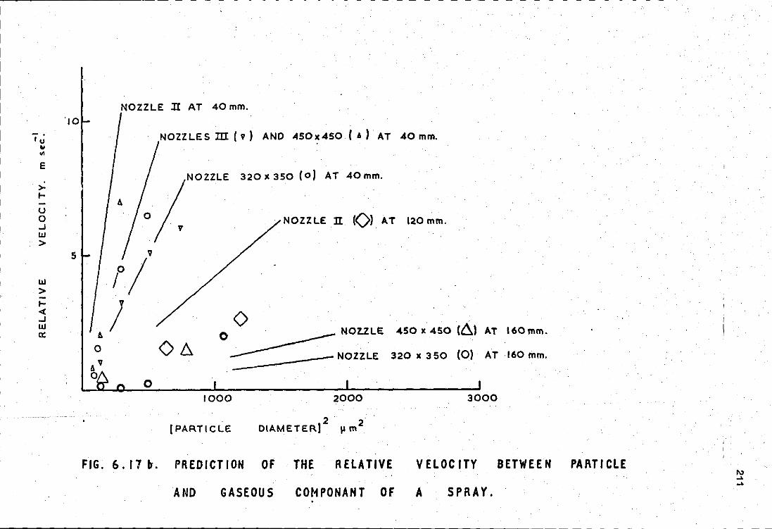
·~ .. "' E
> 1--u 0 ..J w >
Ill > 1-< ..J Ill a:
'10
5
. I
NOZZLE li AT 40 mm.
NOZZLES m (V) AND .450x450 (A). AT 40 mm.
NOZZLE 320 x 350 (o) AT 40mm.
NOZZLE n 101 AT 120 mm.
V
t/ J
~
0 Ob..
0 ' ' 0 · ------ NOZ.ZLE -450 x 450 (6)
-------- . -NOZZLE 320 x 350 (0)
AT l60mm.
AT 160 mm.
0 1000 2000 3000
2 Jl m2 (PARTICLE DIAMETER]
FIG.6.171r. PREDICTION OF THE RELATIVE VELOCITY BETWEEN PAI\TI CLE "' ... ...
AND GASEOUS COt<! PONAN T OF A SPRAY. .
will be less, providing of course that the predicting e~uation 4.1.10
for the velocity of the gaseous component is accurate.
Examining Fig. 6.17 in more detail, it is seen that the agreement·
between theory and data is best at the 80mm range.(Fig. 6.17 (a) ).
At 160mm and 120wm (Fig. 6,17 (b) ) relative velocity measurements tend
to be unreliable because the differences in mean velocity between gas
and particle are generally less than the level of turbulence. Therefore
many more double-flash photographs than those taken would be necessary
212
in order to achieve the required accuracy. At 40mm (Fig. 6.17 (b) ) data
for the three smaller nozzles, 320 x 350, IU and 450 x 450 correlate
reasonably well with the theoretical curve, but the data for the large '
nozzle, II, (not plotted) show no correlation. This is because the
equation predicts relative velocities which would require particles above
about 12p m travelling at a velocity greater than the eXit. velocity.
Thus for large nozzles, of diameter about 0.7mm, the equation, 6.10.5,
is applicable for distances no closer to the nozzle than about 80mm.
For smaller nozzles, up to about 0.5mm diameter, this limit is about 40mm.
The limitations of the above equation with respect to nozzle dimensions
and distance from the nozzle have been considered •. Limitation. regarding
particle size may now be considered. It was stated earlier that this
equation was limited to small particles. The upper limit of the particle
size for which the equation is applicable will now be considered. There
are two factors restricting the upper range of particle size. The first
is that as the size increases, the relative velocity and hence the Reynolds
number of the particle increases. Consequently the Stokes equation no
longer gives the drag force accurately and the latter would be seriously
underestimated. The second factor is that as the relative velocity
increased then the approximation :-
du u ( ~)
g dx
213
loses its validity.
Consider first the effect of an increasing Reynolds number of the
drag force. Stokes equation is applicable for a particle Reynolds number
of less than 0,1, or if a 1o,1o error can be tolerated, less than about 1.
u d Therefore:- rel p < 1 •
Incorporating again the assumption that the gaseous componant
of the spray is mainly air, then:-
the
or < -5 1,8 • 10
1.2 =
-5 1.5.10 2/ . m sec
Thus, the maximum values of.the relative velocity for an error in
drag equation of' no greater than 1o,1o are approximately:-
0.3 m/sec for .a 5011 m particle
0. 75m/sec for a 20p m particle
1 • .5 m/sec for a 1 0 p m particle
It is seen, from Fig. 17 that for particles above about 15 to 20 p·m, the
above criterion is exceeded, exceptatadistance beyond about 160mm from
the nozzle. This is considered later.
Consider the second factor limiting the validity of equation 6.10,5.
This was that u (du /dx) was nolonger approximately equal to u (du /dx). p p g . g
Reference to Fig. 6.16,and Fig. 6.16 (a) especially, reveals that for
35pm particles, for example, the slope (dup /dx) is approximately equal
to or only slightly greater than that' of the gas, beyond about 50 mm from
the nozzle but that the particle velocity, u , may be of the order of p
greater than that of' the gas, u • Thus 35 pm particles may give rise to g
errors of the order of 50%. Consequently the maximum size of particle
for which the error would be again 10%, say, will be similar to that
determined from the Reynolds number criterion.
An explanation is required, therefore, as. to why the relationship
between u 1 and d 2 remains li~ear at particle diameters greater than re p
the limit of 15 - 20 pm determined above.
Refe"rence to equation 6.10.3:-
= d 2 p
offers some explanation as to why the line~r relationship is maintained.
For large particles, both the acceleration term u · (du /dx) and the drag . p p
componant increase simultaneously (but not necessarily proportionately).
As these two terms appear as numerator and denominator respectively in
the equation, it is possible that linearity could be maintained because,
214
over a limited range of particle sizes, their ratio could remain approximately
constant.
An example may be given. -Consider a 35pm particle at 80mm from
nozzle 450 x 450. From Fig.6.16 (a) the deceleration terms for particle
and vapour are:-
du u (-l!)
p dx
du
=-(17 m/sec) (150 /sec)
u (__fi) =-(9m/sec) (130 /sec) g dx
. 2 = -2500 m/sec , and
= -1170m/sec2
Therefore the acceleration term is greater than that given by the approximation,
1 ) -2500 ug (dug 1 dx , by a factor of· _1170 or 2.1.
Now u 1 = 8 m/sec. Therefore the particle Reynolds number, again . re
assuming that the spray consists mainly of entrained air, is approximately:-
d p
air
18
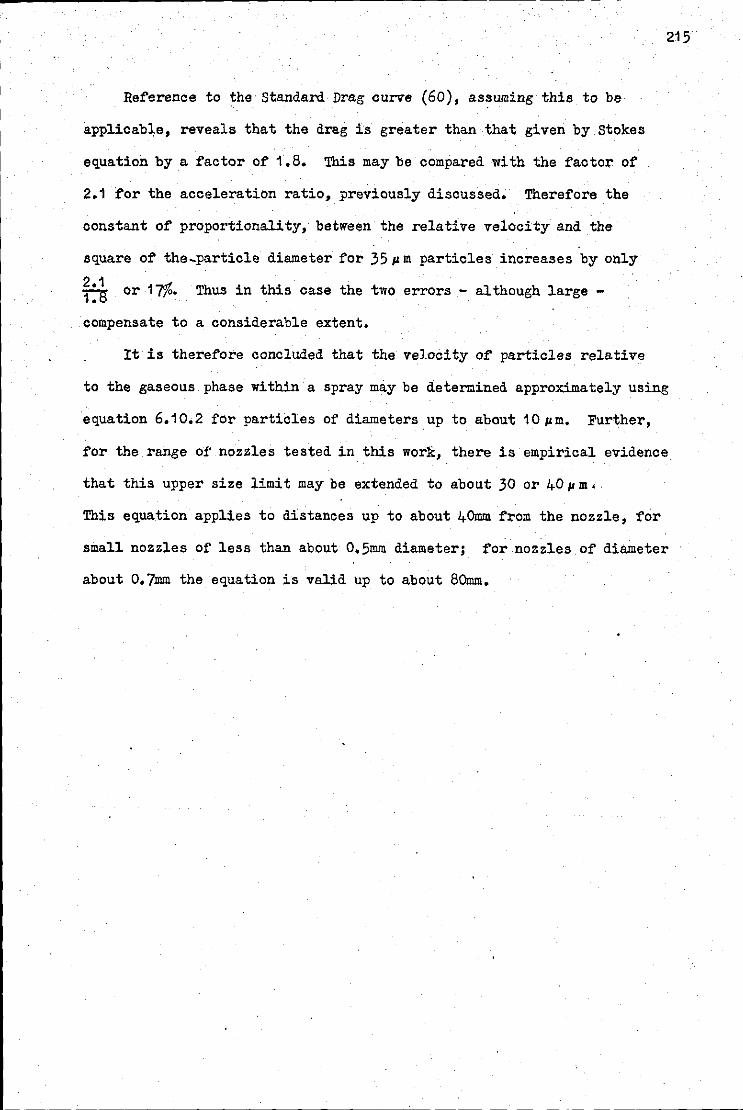
Reference to the Standard Drag curve (60), assuming this to be
applicabl,e, reveals that the drag is greater than that given by stokes
equation by a factor of 1.8. This may be compared with the factor of
2.1 for the acceleration ratio, previously discussed. Therefore the
constant of proportionality, between the relative velocity and the
square of the-particle diameter for 35 p. m particles increases by only
2.1 17% 1:8 Or Oo Thus in this case the two errors - although large -
compensate to a considerable extent.
It is therefore concluded that the velocity of particles relative
215
to the gaseous phase within a spray may be determined approximately using
equation 6.10.2 for particles of diameters up to about 10 p.m. Further,
for the range of' nozzles tested in this work, there is empirical evidence
that this upper size limit may be extended to about 30 or 40 pm'
This equation applies to distances up to about 40mm from the nozzle, for
small nozzles of less than about 0.5mm diameter; for nozzles of diameter
about 0.7mm the equation is valid up to about 80mm.
----------------~- ----

216
6,11 Determination of the size distr·ibution of the resultant surfactant
aerosols and their variation with particle size,
The size distribution of the active ingredient of a spray is of general
interest is aerosol technology, In the case of inhalation therapy this
size distribution among other things determines the effectiveness of
penetration of-the aerosol into the lungs. In this context the most
important parameter regarding the size distribution is then the fraction
by volume between a certain size range; this size range being that which
reaches, and is retained in, the lower recesses of the lungs. Although it
is by no means certain what the precise limits of this range are, there
appears to'be general agreement that particles above about 5pm diameter
will not reach the alveoli,and those of about 0,5pm in diameter will not
be retained, Thus the relevant diameter range is about 0.5 to 5 pm. In
the case of aerosols generated by atomisation of liquids, and by most other
methods, · this lower limit is of little importance because the fraction by
volume below this diameter is usually negligible, Thus the fraction between
0. 5 and 5 pm may be obtained approximately by measuring the fraction below
5 pm,
Size analyses were obtained of the resultant surfactant aerosol·
generated by the atomisation of a solution of propellant and 1% by weight
of the surfactant "span" (or "arlacel") 85. The propellant again consisted
of 60/40 % by weight of propellant 12 and 11 respectively, The concentration
of surfactant, 1% by weight, is tjpical of that used' in commercial practice.
The size analyses are shown in Figs.18(a) and (b), as fraction by
volume below a given particle diameter against .that diameter, The original
data are given in Appendix 1,$. Table 6,5 shovrs mas3 median
diameter (l;:J.!D), volume-surface mean or Sauter mean diameter (Sl<rD) and the
fraction by volume below 5 pm particle diameter.
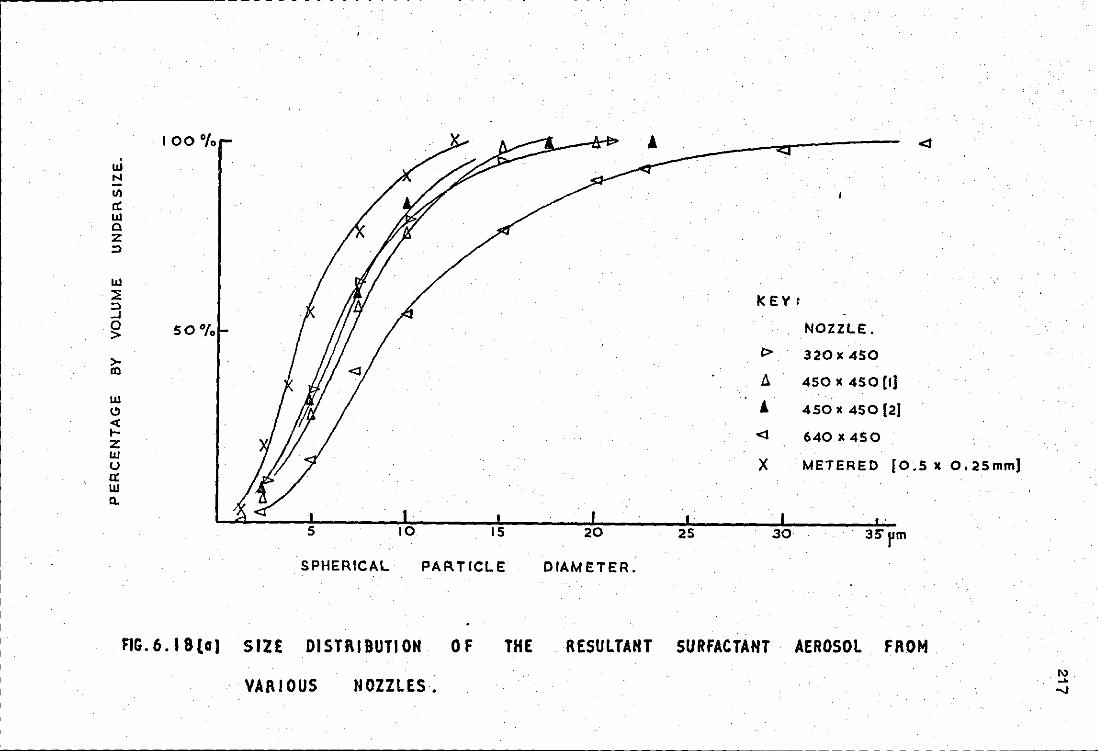
~-------------------------------------------------------------------------------------------------------.
I 00 °/o Ul N
Ill a: Ul a z :;)
Ul :::E :;) kEY: _, 0 SO% > NOZZLE.
>- I> 320X450 m
f:. 450 X 45 0 (I} w Cl ' 450 X 450 (2} < .... z <l 640 X 450 IJJ u 0:
X METERED (0.5 x 0.25mmJ
w CL
25 30
SPHERICAL PAP.TICLE DIAMETER.
AG.6.18{o) SIZE DISTRIBUTION OF THE RESULTANT SURFACTANT AEROSOL FROM
VARIOUS NOZZLES.
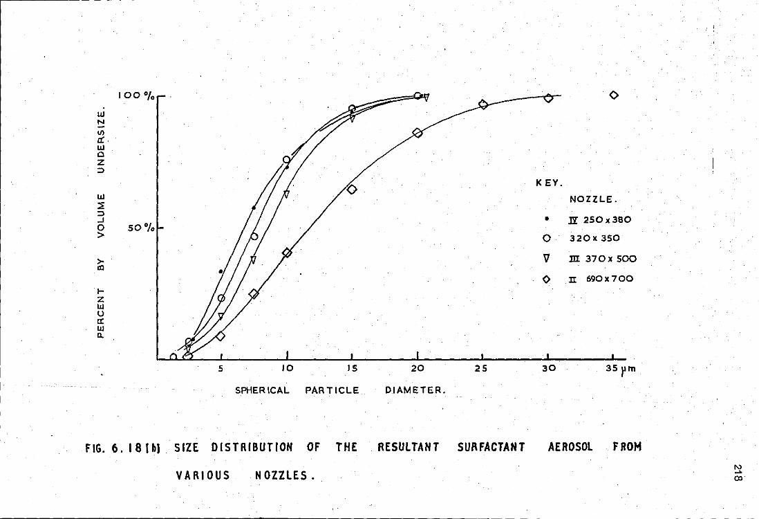
r------------- -- - -- - -- - - - -- - - - - -
. '
100"/o <> UJ N
ll)
a:. UJ a z :::l
KEY. UJ ~
NOZZLE. :::l ...J 0 so%
0 lY 250 l( 380
> 0 320X350
>- V m 370x soo Ill
() II 690X700 1-z l1l u a: UJ a.
5 10 15 20 25 30
SPHERICAL PARTICLE DIAMETER.
FIG. 6. 18 (b) SIZE DISTRIBUTION OF THE RESULTANT SURFACTANT AEROSOL FROM
VARIOUS NOZZLES •
VOLUME-SURFACE NOZZLE MEAN DIAMETER
pm
IV (250 X 380) 5,3
. 320 Jt 350 6. 0
320 Jt 450 5. 2
450 X 450 5, 7 Run 1
450 X 450 5,3 Run 2
640 X 450 6,2
MASS MEDIAN DIAMETER
pm
6,8
7.0
6,6
9.2
640 x· 350 Very large, Not properly atomized.
li (690 X 700)
m (380 x 500)
Metered Spray (500 X 250)
12
8.9
4.8
TABLE 6.5 SIZE ftJrfl~YSES OF THE SOLUTE AEROSOL
PERCENT BY VOLUME BELOW
5f.lm
24
35
28
32
16
8.0
16
55
219
220
In Fig.19 the mass median diameter is plotted against the diameter
of the do1mstream nozzle. It is seen that for nozzles whose orifices are
of similar diameter, the relationship between mass median diameter and
-2 orifice diameter is tolerably linear. The slope is 1.6 :x: .1 0 •
Therefore:-
Mass median diameter= 1.6 x 10⁻² x (orifice diameter).
Similarly:-
Volume surface mean diameter = 1. 2 x 10.:...2 x {orifice diameter)
Also the fraction by volume below 5 lA m particle diameter is given, very
roughly, by:-
Fraction below 5 .u m :::!:!::: 0.17 ( 1 ; D)
. where D is orifice diameter in mm.
For nozzles whose diameters are not equal, two cases may be considered.
Firstly, when the upstream orifice is smaller than the downstream, there
is some evidence to suggest that atomization is marginally improved. This
is to be expected because as this first orifice becomes smaller, the
temperature fall across it rises and the mass fraction of propellant
evaporated increases. Thus a propellan~ of higher gas-to:vapour ratio is
presented to the final, downstream, orifice.
When the upstream orifice is larger than the downstream, atomization
efficiency deteriorates rapidly. Thus, compared with a mass median diameter
of 7.0 ~Am for the 450 :x: 450 nozzle, that of the 640 :x: 450 nozzle was 9.2 pm,
while the 640 x 350 nozzle failed to atomize properly, producing pools of
surfactant on ths microscope slides. Indeed during one run in the determination
of mass flmv-rate, this nozzle produced a stream of unatomized propellant.
From consideration of the geometrical configuration of the nozzle this is
perhaps to be expected because the two orifices are in line and it is
possible therefore, as with any of these nozzles, for propellant to pass
,----------- -- - - -- - - --- -- - - -- --------------------- -- -
a: UJ .... UJ ::E < 0
z < -0 UJ ::E
Cl)
Cl)
< ::E
10-pm
5
FIG • 6. 19 • VARIATION
NOZZLE:
0 690X 700
/-~--CORRELATION FOR. NOMINALLY
640 X 450 0 o 380x 500
320x3SO o. / 250 X JBO O 0 450X450(1)
/
0 450X450(2) 0 320X 450
.0 METERED SPRAY soox 250
300 400 500 600
DIAMETER OF DOWNSTREAM ORIFICE.
TWIN ORIFICE NOZZLES.
700pm.
0 F AEROSOL SIZE DISTRIBU.TION Wl TH NOZZLE DIAMETER.
N N .....
222
directly in litr.lid fonn from one orifice to the other. In the case when
the first orifice is larger than the. second however, this tendency is
considerably enhanced because the required temperature fall across this
first orifice, and hence propellant evaporation, are substantially reduced,
This explanation is supported by data from the metered spray, This has
the same ratio of upstream to downstream orifice diameter but produces a
very fine spray. Further the parameters of the size distribution of this
spray correlate well with those of the continuous sprays whose orifices
are of similar diameter.
223
6.12 t!etastabiliti
It was stated in Section 4 that the propellant in the expansion
chamber was in a metaatable state, at a pressure which was generally
lower than the S. V.P. corresponding to ita temperature.. .An expression
for the degree of metaatability was determined· empirically~ Defining the
degree of metastability,liP t, as the difference between the S.V.P. · . me a
ot propellant at expansion chamber temperature minus the expansion c~amber
pressure, or
liP = meta SVPTe , then the empirical expression
D 2.5 1
This is shown in Fig. 6.20, together with experimental values of liP t me a.
These were obtained from data given in Appendix 1.3.
In using this equation the value of the expansion chamber temperature
Te , with which to determine the S. V. P., may be obtained approximately
from a simplified relationship for the temperature fall across .the first
orifice; this is given insub-section 6.3.
0! KEY. w EMPIRICAL EXPRESSION FOR: Dl .. 320p . dl 50
Dl ::E < • 250 .. m J: u 0 320
40 1::. 450 6 z
0 0 700 -
Ill z
D1•450pm < a. 30
X w
1-z 20 < "' ..J ,. ..J E o
1• 750 pm w z a.
"" 0 a. 10 a.
w u. a: 0 ::l
Ill a. Ill
>: w er •10 •IS •20 x ro-12 m 4
Ill a.
( DOWNSTREAM ORIFICE)4
·
FIG. 6. ZO. METASTABILITY OF THE PROPELLANT I N THE E XPAN SI ON CHAMBER. 1\)·
"' .,..
225
7 CONCLUSIONS .AND RECm.!J.IENDATIONS FOR FURT!BR WO~
7.1 Conclusions
A theoretical expression has been produced by means of which it is
possible to predict the axial velocity of the·gaseous component of a continuous
.spray generated by passing a liquified-gas prop~llant through a two-orifice·
nozzle assembly. From this expression values for off-axis velocities may
be determined by assuming a Gaussian transverse distribution of velocity.
Also an approximate value of the velocity of the particulate component of
the spray may be obtained from a relationship determined semi-empirically,
between particle diameter and the relative velocity between particle and
gaseous component.
The primary expression, referred to above, requires three independently
determined empirical factors. They are the position of the apparent
origin of the spray, the angle of divergence of the spray and the degree
of metastability of the propellant in the expansion chamber of the nozzle
assembly. The first of these, the position of the apparent spray-origin,
.was determined photographically, It is taken as 30mm upstream of the
nozzle for twin-orifice nozzles; its value for other nozzle.astemblies is
discussed in Section 6. The divergence angle was shown to be approximately
equal to that of an air jet. Finally the degree of metastability is given
by a simple expression in terms of the orifice dimensions and the S.V.P.
of the propellant; generally metastability appears as a small correcting
term.
The development of the predicting equation for axial velocity
required the following subsidiary expressions. They were expressions
for the mass flow-rate of propellant through the upstream and downstream
orifices (short tubes)-, the mass flow-rate through a two-orifice nozzle
assPmbly, the temperature and hence the quality of propellant in the
expansion chamber, and also the exit velocity of the spray. The expressions
226
for the mass flow-rate through the downstream orifice and exit velocity,
also from the dovmstream orifice, were based on the assumption of' mass-limiting
flow.
Experimental support f'or the primary expression was given for three
nominally twin orifice nozzles of' orifice diameter 0.33mm , 0.45mm and 0.60mm.
Experimental support f'or the subsidiary expressi·ons was given f'or orifice
diameters ranging from 0,25mm to 0.70mm and orifice diameter ratios from
about 0.5 to 2,0, although exit velocity data were available for only
part of' this range.
A feature of' the expressions developed was that without undue loss
of accuracy, they could generally be reduced to simple functions of' orifice
diameters D1
, D2
; thus trends are readily predictable. They are applicable
for a propellant, at 20°C, consisting of', by weight, 6Cifb propellant 12, 4Cifb
propellant 11, with a solute "Span 85", 1% by weight. These simplified
expressions are listed below
1. Mass flow-rate (i!)::!:!: 6.6 x 1o3 D1D2 kg/sec
2. Temperature fall across the upstream orifice (~T1 )
3.0 D 2 (2)
D1 deg C.
3. Quality of' propellant (mass fraction evaporated) in the expansion chamber(q)
4.
o. 018
Mean velocity of' gaseous componant of' the spray (u ) ga
1 2
(x + z) tana ,.,. J 2 2 . 2
. e(-y /x tan a )
227
Here J is the momentum efflux whose determination was discussed in
Section 4• Also, x and y are downstream and off-axis distances
respectively, and o is the 1/e- velocity half-angle.
5. Axial particle velocity is given by:-
uga (1 +(~unction(dp2 )))
where (function (dp2))was discussed in Section 6,
6. A furth~r, empirical, expression was derived for the mass median diameter
(MMD) of the spray of residual solute, "Span 85", generated by nominally
twin orifice nozzles, This was:-
where D is the orifice diameter, Distributions from.some dissimilar
orifice nozzles were given in Section 6.
The above equations, and their more precise forms given in Section 6,
generally enable spray properties to be determined in terms of fundamental
parameters, They also are of assistance in the design of inhalation devices.
In this respect it is clear from the above, that in order to produce a spray
suitable for inhalation therapy the orifice diameters should. be as small
as possible. This has the dual advantage that both spray size and velocity
are minimised, It could possibly be advantageous, however, to use a nozzle
assembly whose ratio, D2 :D1, was greater than 1; this would improve the
quality of the propellant in the expansion chamber. However limited.
evidence available suggests that, with respect to particle size, the diameter
of the downstr0am orifice is the overiding factor 11hen this orifice is the
larger. Thus it is considered that both diameters should be reduced to a
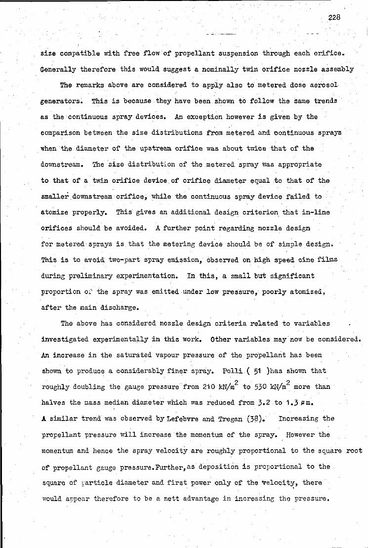
228
size compatible with free flow of propellant suspension through each orifice.
~enerally therefore this would suggest a nominally twin orifice nozzle assembly
The remarks above are considered to apply also to metered dose aerosol
generators. This is because they have been shown to follow the same trends
as the continuous spray devices. A.~ exception however is given by the
comparison between the size distributions from metered and continuous sprays
when ·the diameter of the upstream orifice was about twice that of the
dovmstream. The size distribution of the metered spray was appropriate
to that of a twin orifice device. of orifice diameter equal .to that of the
smaller.downstream orifice, while the continuous spray device failed to
atomize properly. This gives an additional design criterion that in-line
orifices should be avoided. A further point regarding nozzle design
for metered sprays is that the metering device should be of simple design.
This is to avoid two-part spray emission, observed on high speed cine films
during preliminary experimentation. In this, a small but significant
proportion o.:· the spray was emitted under low pressure, poorly atomized,
after the main discharge.
The above has considered nozzle design criteria related to variables
investigated experimentally in this work. Other variables may now be considered.
An increase in the saturated vapour pressure of the propellant has been
shown to produce a considerably finer spray. Polli ( 51 )has shown that
2 2 roughly doubling the gauge pressure from 210 k}T/m to 530 kN/m more than
halves the mass median diameter which was reduced from 3.2 to 1.31'm.
A similar trend was observed byLefebvre and Tregan (38). Increasing the
propellant pressure will increase the momentum of the spray. However the
momentum and hence the spray velocity are roughly proportional to the square root
of propellant gauge pressure.Further,as deposition is proportional to the
square of ,·article diameter and first power only of the velocit~, there
would appear therefore to be a nett advantage in increasing the pressure.
229
Spray angle may next be considered. Generally the greater the
divere;ence angle of' the spray the greater is the attenuation of spray
velocity. Also, the greater is entrainment of air which wotud promote
evaporation of the droplets. Thus it would appear advantageous to increase
the spray angle, although operation in the confined region of the mouth
would considerably modify the above mbdel.
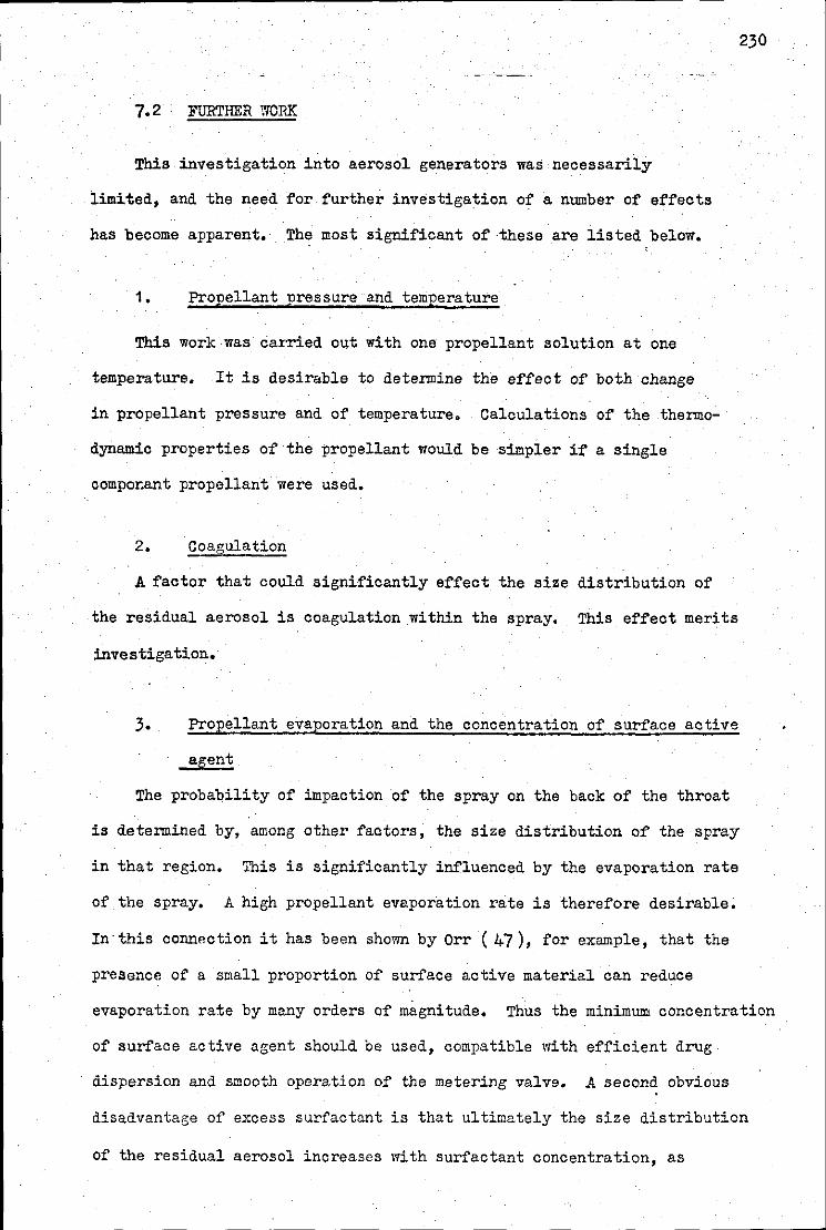
7.2 FURTHER WORK
This investigation into aerosol generators was necessarily
limited, and the need for further investigation of a number of effects
has become apparent. The most significant of·these are listed below.
1. Propellant pressure and temperature
This work was carried out with one propellant solution at one
temperature. It is desirable to determine the effect of both change
in propellant pressure and of temperature. Calculations of the thermo
dynamic properties of the propellant would be simpler if a single
compor.ant propellant were used.
2. Coagulation
A factor that could significantly effect the size distribution of
the residual aerosol is coagulation within the spray. This effect merits
investigation.
3. Propellant evaporation and the concentration of surface active
agent
The probability of impaction of the spray on the back of the throat
is determined by, among other factors, the size distribution of the spray
in that region. This is significantly influenced by the evaporation rate
230
of the spray. A high propellant evaporation rate is therefore desirable.
rn·this connection it has been shown by Orr ( 47 ), for example, that the
presence of a small proportion of surface active material can reduce
evaporation rate by many orders of magnitude. Thus the minimum concentration
of surface active agent should be used, compatible with efficient drug
dispersion and smooth operation of the metering valve. A second obvious
disadvantage of excess surfactant is that ultimately the size distribution
of the residual aerosol increases with surfactant concentration, as
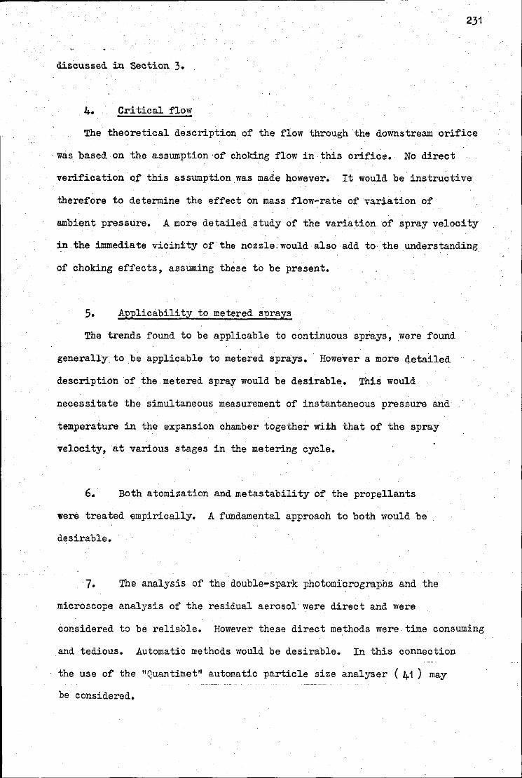
231
discussed in Section 3.
4. Critical flow
The theoretical description of the flow through the downstream orifice
was based on the assumption·of choking flow in this orifice. No direct
verification or this assumption was made however. It would be instructive
therefore to determine the effect on mass flow-rate of ;ariation of
ambient pressure. A more detailed study of the variation of spray velocity
in the immediate vicinity of the nozzle. would also add to the understanding
of choking effects, assuming these to be present.
5. Applicability to metered sprays
The trends found to be applicable to continuous sprays, .were found
generally. to be applicable to metered sprays. However a more detailed
description of the metered spray would be desirable. This would
necessitate the simultaneous measurement of instantaneous pressure and
temperature in the expansion chamber together with that of the spray
velocity, at various stages in the metering cycle.
6. Both atomization and metastability of_ the propellants
were treated empirically. A fundamental approach to both would be
desirable.
7. The analysis of the double-spark photomicrographs and .the
microscope analysis of the residual aerosol were direct and were
considered to be reliable. llowever these direct methods were time consuming
and tedious. .Automatic methods would be desirable. In this connection
the use of the "Quantimet" automatic particle size analyser ( 41 ) may
be considered.
8, The work has dealt with one facet of the study of inhalation
therapy. It has shovm that in all probability, the main factor limiting
the efficiency of liquified gas aerosol generators is the minimum size
of the nozzle diameters,, This will be limited by their tendancy to clog
during operation with powder suspensions. Therefore future work should
perhaps be concentrated on this aspect at the study, The possible use
of propellant vapour as an alternative means of powder dispersion may
profitably be investigated, The advantages in terms of rapid. velocity
decay have been demonstrated,
232
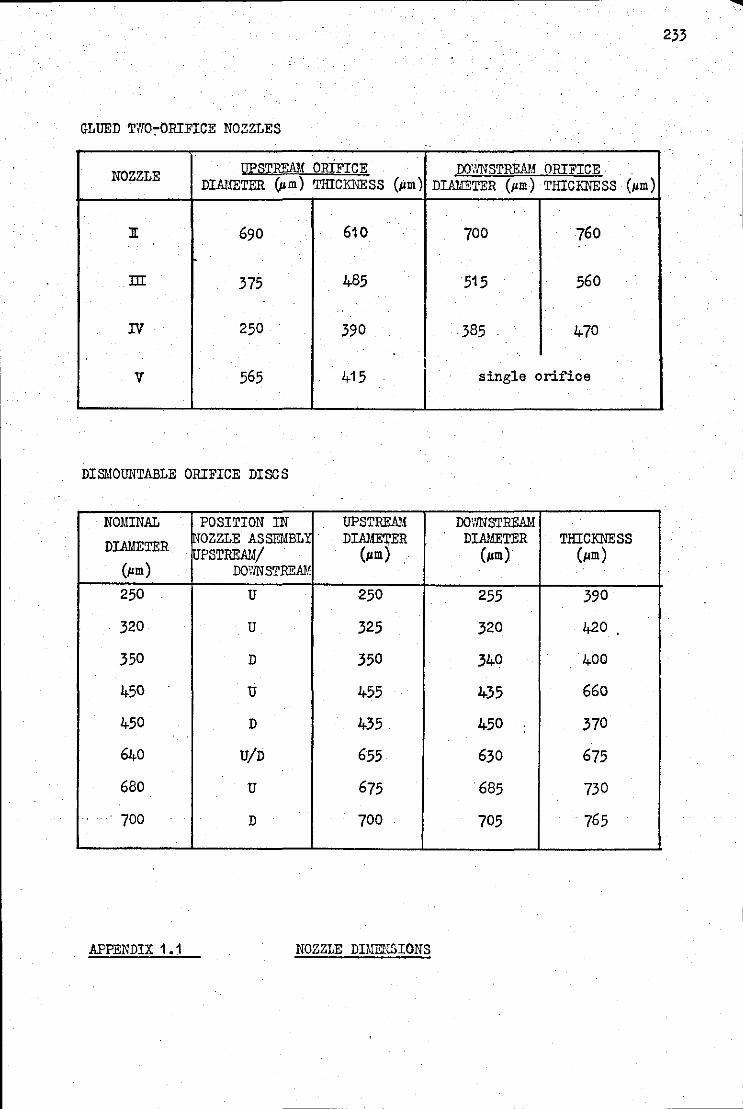
233
GLUED THO~ORIFICE NOZZLES . .
NOZZLE ll.:ESTRJW.! ORIFICE DOWNSTREAM ORIFICE DIAI.!ETER (.u m) THICKNESS (pm) DIAI.!ETER (pm) TillCKNESS (pm)
:n: 690 610 700 760
m 375 485 515 560
rr 250 390 . 385 470
I V 565 415 single orifice
DISMOUNTABLE ORIFICE DISCS
NOMINAL POSITION IN UPSTREAI! DOWNSTREAM
DIA!.!ETER !NozzLE ASSEMBLY . DIAMETER DIAI.!ETER THICKNESS iuPSTREAIJ/ (pm) (pm) (pm)
(pm) DOWNSTREAI.!
250 u 250 255 390
320 u 325 320 420 .
350 D 350 I 340 400
450 u 455 435 660
450 D 435 450 370
640 U/D 655 630 675
680 u 675 685 730
. 700 D 700 705 765
APPENDIX 1 .1 NOZZLE DHrENSIONS
NOZZJ,E .
250 X 350
320 X 350
320x 450
320 X 700
450 X 350 .
450 X 450
450 X 700
680 X 350 .
680 X 450 .
680 X 700
APPENDIX 1 • 2 ·
TEMPERATURE gF MEAN DISCHARGE RATE PROPELLANT ( C) STANDARD DEVIATION
20.7
20.9
20.9
20.5
20.8
20.4
20.6
20.7
20.7
20.7
MASS FLO'Y RATE
STANDARD ERROR OF THE MEAN ( gfsec~)
.57
.02
.01
.77
.oo
.oo
.99
.02
.015
1. 31 .05 .03
1.17 .04 .03
1.42 .02 .01
.
1.88 .02 .01
1.56 *
2.08 .06 .04
2.84 .02 .015
* One reading only. During the second run, the propellant streamed undispersed, from the nozzle.
234
·.
NOZZLE 250 X 350 320 X 350 320 X 450 320 X 700 450 X 450 450 X 700 640 X 350 640 X 4,50 680 X 700
MEAN UPSTREAM PRESSURE PRIOR TO SPRAYING 408 413 414 410 411 408 414 414 403 kN/m2 (abs)
MEAN UPSTREAM PRESSURE (RillJNING) Pi kN/m2 (abs) 407 410 413 404 406 400 407 408 400
.
MEAll EXPANSION CHAMBER PRESSURE 336 350 324 245 364 303 400 387 359 p ¥-.N/m2 ( abs) . e
ME/IN UPSTREAM TEMPERATURE 19.55 I 19.7 20.1 20.6 20.0 20.3 20.4 20.1 20.15 T. °C J. I .
MEAN EXPANSION CHAMBER TEMPERATURE 14.3 16 14.7 9.6 17.1 14.1 19.8 18.7 17.5 T °C e
PRESSUP~ DIFFERENCE ACROSS UPSTREAM ORIFICE ( AP1 )kN/m2 (abs)
Mean 71 60 88 162 41.2 96 7.6 22 40 Standard deviation .7 10 11 3 2 2 2 .7 3 standard error of mean .4 4 7 2 1. 5 1 1 .5 1.5
TEMPERATURE DIFFERENCE ACROSS UPSTREAM ORIFICE ( AT1 ) deg C
Mean 5.2 :;.6 5.3 11 2.9 6.2 0.56 1.3 2.6 Standard deviation 0.1 .25 .1 .1 .1 .1 .1 .1 .25 standard error of mean 0.05 .1 . .07 .07 .07 .07 .05 .07 ·1
I CORRECTED TEMPERATURE DIFFERENCE 5.9 4.2 . 5.8 1 o. 8 3.4 6.:; 0.7 1. 6 2.9 .AT1"' deg C
.
APPENDIX 1.3 TEMPERATURR AND PRESSURE MEASUREMENTS OF THE PROPELLANT DURING NOZZLE FLm'l
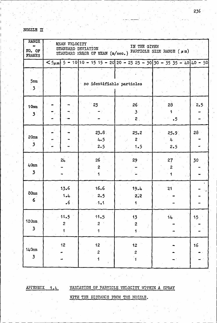
236
NOZZLE tr
RANGE .
- MEAN VELOCITY IN THE GIVEN
NO. OF STANDARD DEVIATION (Pm) STANDARD ERROR OF MEAN (m/sec.) PARTICLE SIZE RANGE
FRAMES
. <5,um 5 - 10 10 - 15 15 - 20 20- 25 25 - 30 30- 35 35- 40 40 - 50 -
5mm no identifiable particles
3
10mm - - 23 26 28 2.5 I - - - 3 1 -3 - ·- - 2 .5 -
- - 23.8 25.2 25.9. 28 20mm
4-5 2 4 -- -:3 - - 2.5 1.5 2.5 -
.
.
24 26 29 27 30 40mm . - 2 - 2 -
3 - 1 - 1 -
13.6 16.6 19.4 21 -80mm '
1.4 2.5 2~2 - -6 .6 1.1 1 - -
.
. 11.5 11.5 13 14 15 120mm 2 2 2 - -
3 1 1 1 - -12 12 12 - 16
140mm I 2 2 - --3 - 1 1 --
APPENDIX 1 • 4 VAPJATION OF PARTICLE VELOCITY VITTHIN A SPRkY
VIITH THE DISTANCE FROM THE NOZZLE.
------------------ - - - - -
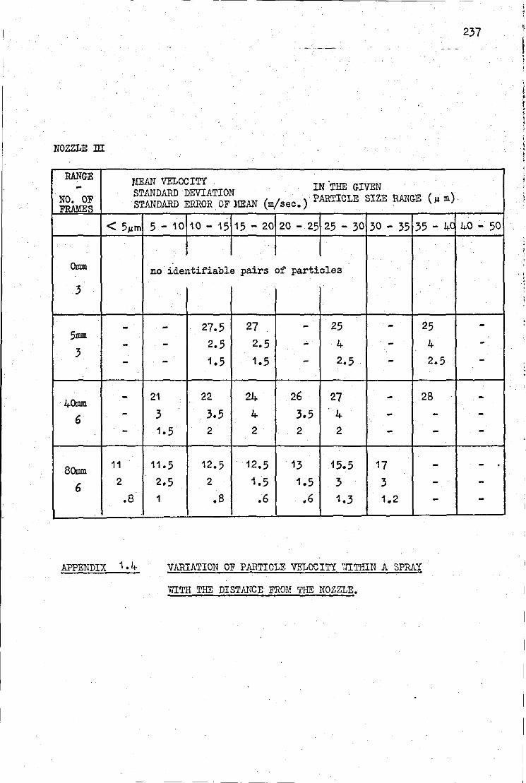
NOZZLE m
RANGE MEAN VELOCITY . ~ IN.THE GIVEN
NO. OF STANDARD DEVIATION "' ) ST.IillDARD ERROR OF l!EAN' (m/sec.) P.AR~ICLE SIZE RJ;NGE ( 1-1 m
FIW!ES
< 5pm 5- 10 10 - 15 15- 20 20 - 25 25 - 30 30- 35 35- 4C
. .
Omm no identifiable pairs of particles
3
- - 27.5 27 - 25 - 25 5mm - - 2.5 2.5 - 4 - 4 3
- - 1.5 1.5 - 2.5 - 2.5
- 21 22 24 26 27 - 28 40mm 6 - 3 3.5 4 3.5 4 ~ -
- 1.5 2 2 2 2 - -
80mm 11 11.5 12.5 12.5 13 15.5 17 -6 2 2.5 2 1.5 1.5 3 3 -
.8 1 .8 .6 .6 1.3 1.2 -.
APPENDIX 1 • 4- VARIATION OF PARTICLE VELOCITY ';/IT!ITN A SPRAY
WITH THE DISTANCE FROM THE NOZZLE.
237
40 - 50
---
---
- . --
~ t ; ' ' ; ' I ;
t
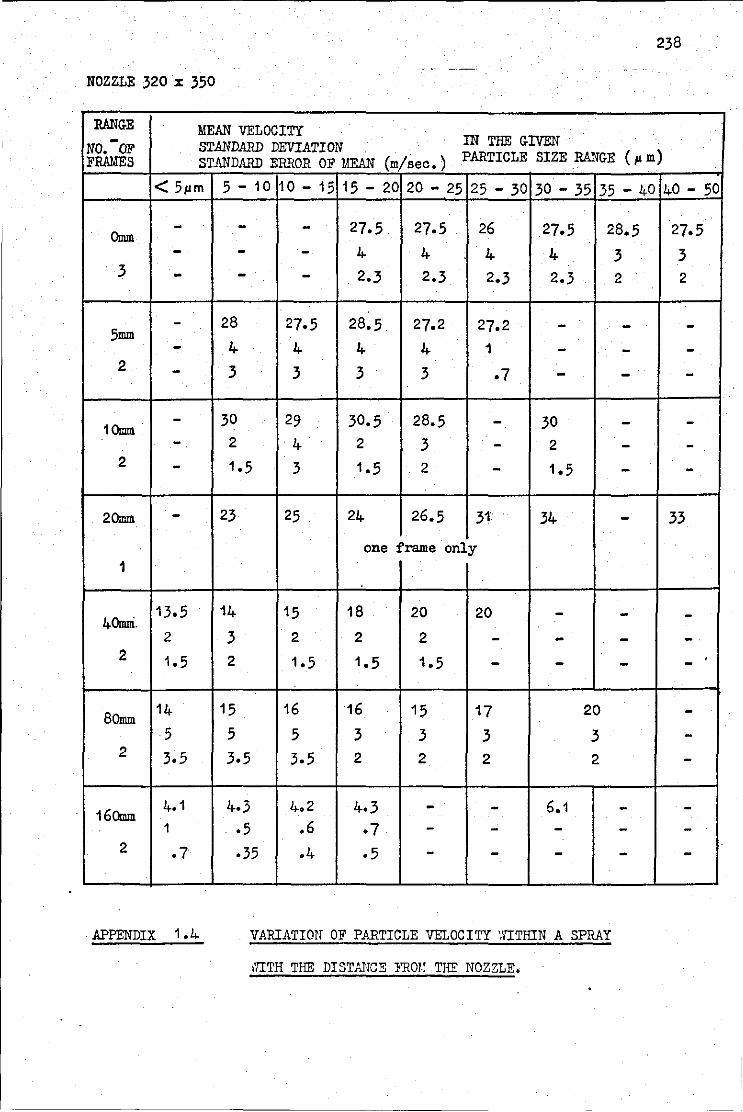
238
NOZZLE 320 x 350
RANGE MEAN VELOCITY NO.-OF STANDARD DEVIATION IN THE GIVEN FRAMES ST11NDARD ERROR OF MEAN (m/sec.) PARTICLE SIZE RANGE (!I m)
< 5.um 5 - 10 10 - 15 15- 20 20 - 25 25 - 30 30 - 35 35- 40 40- 50 .
- - - 27.5 27.5 26 27.5 28.5 27.5 Omm - - - 4 4 4 4 3 3 3 - - - 2.3 2.3 2.3 2.3 2 2
. .
- 28 27.5 28.5 27.2 27.2 - - -5mm - 4 4 4 4 1 - - -2 - 3 3 3 3 .7 - - -
- 30 29 30.5 10mm 28.5 - 30 - -- 2 4 2 3 - 2 - -
2 - 1.5 3 1.5 2 - 1.5 - -.
20mm - 23 25 24 26.5 31 34 - 33
one frame only 1
40mni. 13.5 14 15 18 20 20 - - -2 3 2 2 2 - - - -
2 1. 5 2 1.5 1.5 1.5 . - - - -
80mm 14 15 16 16 15 17 20 -5 5 5 3 3 3 3 -
2 3.5 3.5 3.5 2 2 2 2 -
160mm 4.1 4.3 4.2 4.3 - - 6.1 - -1 .s .6 ·7 - - - - -
2 .7 ·35 .4 .5 - - - - -.
APPENDIX 1 • 4 VAPJ:ATIOII OF PARTICLE VELOCITY '.'/!THIN A SPRAY
I'IITH THE DIST!JICE :B'ROI;! THE NOZZLE.
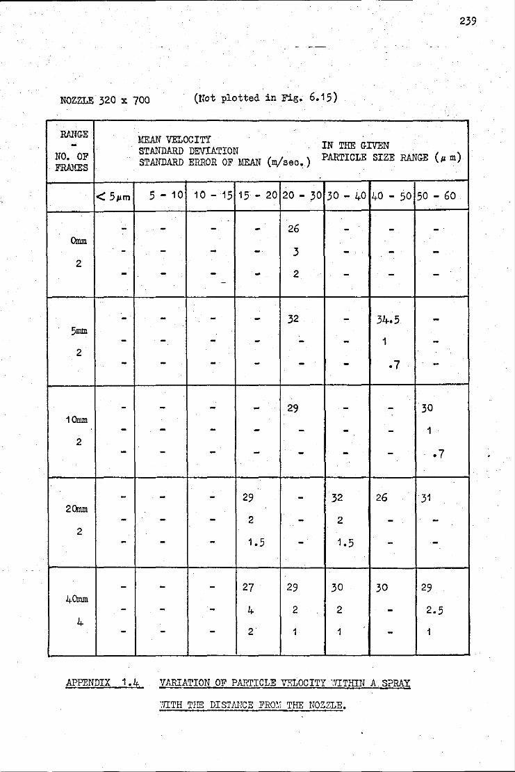
239
NOZZLE 320 x 700 (Uot plotted in Fig. 6.15) .•
Rf,NGE MEAN VELOCIT'I ... IN THE GIVEN
NO. OF STANDARD DEVIATION PARTICLE SIZE RANGE (I' m) STANDARD ERROR OF MEAN (m/sec.) FRAMES
.
< 5pm 5 - 10 10 - 15 15 - 20 20- 30 30- 40 40 - 50 50 - 60
- - - - 26 - - -Omm - - - - 3 - - -2 - - - - 2 - - --
- - - - 32 - 34.5 -5mm
- - - - - - 1 -2
- - - - - - .7 -. - - - - 29 - - 30
10mm - - - - - - - 1 2 - - - - - - - .7
.
- - - 29 - 32 26 31 20mm
- - - 2 - 2 - -2
- - - 1.5 - 1.5 - -
- - - 27 29 30 30 29 40mm
- - - 4 2 2 - 2.5 4
- - - 2 1 1 - 1
APPENDIX 1. 4 V.ARIATION OF PA.'lTICLE VF.LOCITY '.'/!THIN A. SPRAY
7/ITH THE DISTAI,CE FRm! THE NOZZLE.
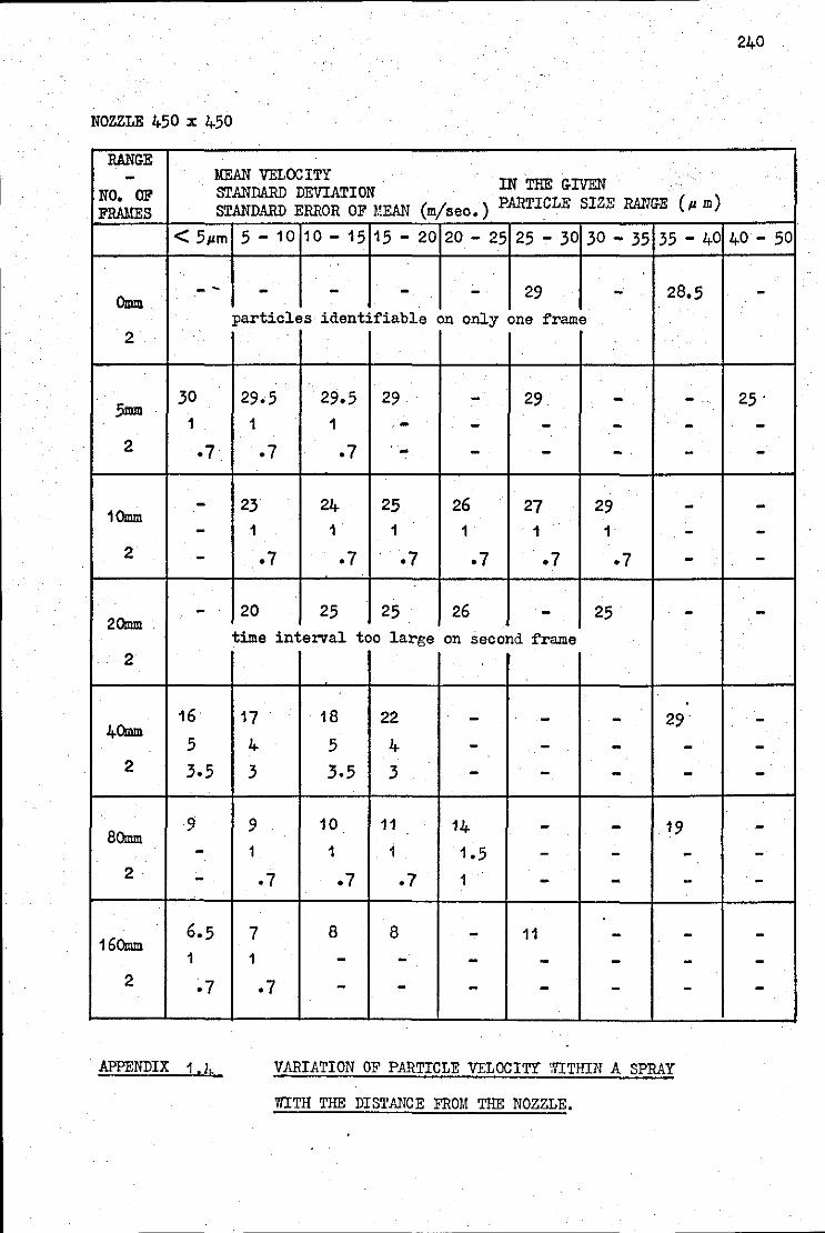
240
NOZZLE 450 x 450
RANGE - MEAN VELOCITY IN THE GIVEN NO. OF STANDARD DEVIATION
( 11 m) FRAMES STANDARD ERROR OF MEAN (m/sec.) PARTICLE SIZE .RA1lG·E
< 5pm 5- 10 10 - 15 15 - 20 20- 25 25 - 30 30- 35 35 - 40 40- 50
-- - - - - 29 . - 28.5 -Omm particles identifiable on only one frame
2 .
.
.
30 29·5 29.5 29 - 29 - - 25. .5mm
1 1 1 - - - - - -2 ·1 .7 .7 - - - - - -
- 23 24 25 26 27 29 - -10mm - 1 1 1 1 1 1 - -2 - .7 .7 ·1 .7 .7 .7 - -
- 20 25 25 20mm
26 - 25 - -time interval too large on second frame
2
16 17 18 22 - - . - 29 -40mm 5 4 5 4 - - - - -
2 3.5 3 3.5 3 - - - - -9 9 10 11 14 - - 19 -80mm - 1 1 1 1.5 - - - -
2 - .7 .7 .7 1 - - - -
6.5 7 8 8 - 11 - - -160mm 1 1 - - - - - - -
2 ~7 .7 - - - - - - -.
APPENDIX 1 , 4 VARIATION OF PARTICLE VELOCITY '.VITHIN A SPRAY
WITH THE DISTANCE FROM THE NOZZLE.
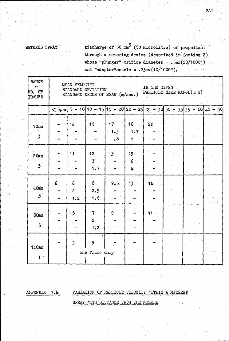
----------------------------------------------------------------------~- '
'METERED SPRAY
RANGE ....
~0. OF ""'"""S
241
Discharge of 50 mm3 (50 micrclitre) of propellant
through a metering device (described in Section 2)
whose "plunger" orifice diameter = .5mm(20/1000")
and 11adapter11 nozzle = .25mm{10/1000"),
MEAN VELOCITY IN THE GIVEN STANDARD DEVIATION PARTICLE SIZE RANGE(!' m) STANDARD ERROR OF MEAN (m/sec.)
< 5pm 5.- 10 10 - 15 15- 20 20 - 25 25 - 30 30 - 35 · ..
35 - 40 40- 50
10mm - 14 15 17 18 20
- - - 1.3 1. 7 -3 - - - .a 1 -
20mm - 11 12 13 19 -- - 3 - 6 -
3 - - 1, 7 - I 4 -
6 6 8 9.5 13 14 40imll - 2 2.5 - - -
3 - 1.2 1.5 - - - .
80mm - 5 7 9 - 11
- - 2 - - -3 - - 1.2 - - - .
- 3 9 - - -140mm
one frame only 1 I I
APPENDIX 1,4 VAlUATION OF PARTICLE VBLOCITY ·:/ITIDN A METERED
SPRAY I'IITH DISTANCE FROM THE NOZZLE
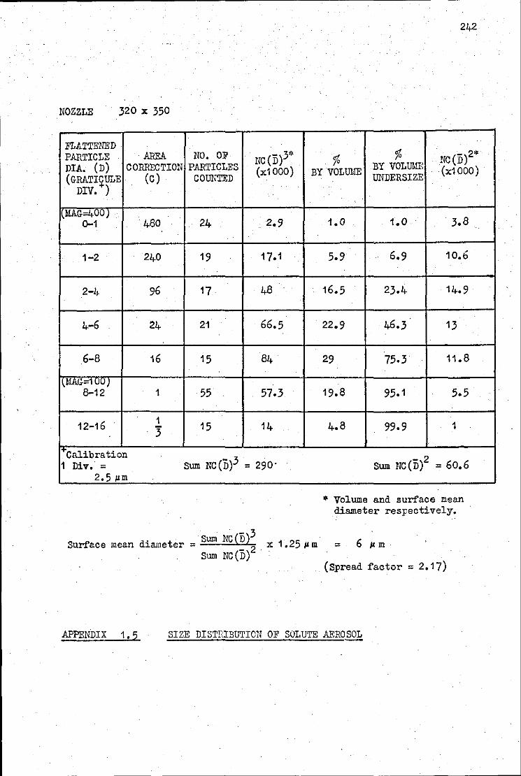
242
NOZZLE 320 X 350
FLJ.TTENED PARTICLE AREA NO. OF NC (i5)3* % % NC (ii)2* DIA. (D) CORRECTION PARTICLES (x1 000) BY VOLUME BY VOLUME (x1000) (GRATI~ULE (C) COUNTED UNDERSIZE
DIV. )
MAG=4UUJ Q-1 480 24 2.9
.
1-2 240 19 17.1 .
2-L~ 96 17 48
-
4-6 24 21 66.5
6-8 16 15 84
1
lMAG--'1 u~ J 8-12 1 55 57.3
1
1 12-16 3 15 14
Calibration sum NC(n)3 = 290· Div.· =
2.5 pm
Surface mean diameter = Sum NC (iS)~ x 1. 25 pm Sum Nc(ii) ·
1.0 1.0 3.8
5.9 6.9 10.6
16.5 23.4 14.9
22.9 46.3 13
29 75.3 11.8
19.8 95.1 5.5
.
4.8 99.9 1
- 2 Sum NC(D) = 60.6
• Volume and surface mean diameter respectively.
= 6 I' m
(Spread factor= 2.17)
APPENDIX 1 • 5 SIZE DISTRIBUTION OF SOLUTE AEROSOL
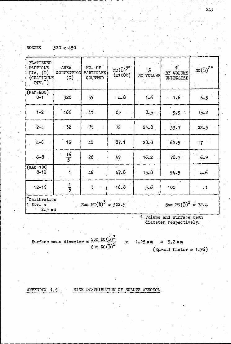
NOZZLE 320 X 450
FLATTENED PARTICLE AREA DIA. (D) CORRECTIO! (GRATICULE
DIV. +) (C)
(MAG=400) D-1 320
1-2 160 .
2-4 32
4-6 16
6-8 16 3
IT MAG=1 Od) 8-12 1
12-16 1 5
+calibration 1 Div. =
2. 5 pm
NO. OF NC(ii)3* PARTICLES (x1 000) COUNTED
59 4.8 .
41 25
75 72
42 87.1
26 49
46 47.8
3 16,8
Sum NC(ii)3 = 302.5
243
.
% % Nc(iif• BY VOLUME BY VOLUME
UNDERSIZE
1.6 1,6 6.3
8.3 9-9 15.2
23.8 33.7 22.3
28.8 62.5 17
16,2 78.7 6.9 .
15.8 94.5 4.6
5.6 100 .1
Sum NC(ii)2 = 72.4
* Volume and surf'ace mean diameter respectively.
Sum NC(D)3 Surface mean diameter=- 2 x 1.25pm = 5.2pm
Sum NC(D) (Spread factor= 1.96)
APPENDIX 1 , 5 SIZE DISTRIBUTION OF SOLUTE AEROSOL.
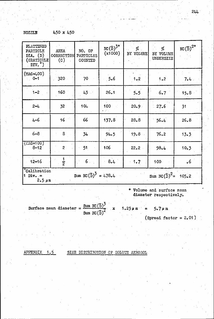
NOZZLE 450 X 450
FLATTENED NC(ii)3* PARTICLE AREA NO. OF DIA, (D) CORRECTION PARTICLES (x1000) (GRATICULE (C) COUNTED
DIV.+)
(MAG-=400) Q-1 320
.
70 5.6
~
1-2 160 43 26.1 .
2-4 32 104 100 ...
4-6 16 66 137.8
6-8 8 34 94.5
I ( t:AG-=1 00 ) 8-12 2 51 106
12-16 1 6 8.4 2 1 +Calibration
Sum NC(ii)3 = 478.4 1 Div •. = 2.5 pm
Surface mean diameter= Sum NC(~)~ Sum NC(D)
X
I
244
% % NC(n)2* BY VOLUME BY VOLUME
UNDERSIZE
1.2 1.2 7.4
5.5 6.7 15.8
20.9 27.6 31
28.8 56.4 26,8
19.8 76.2 13.3
22.2 98.4 10.3
1. 7 100 .6
Sum NC(n)2= 105.2
* Volume and ·surface mean diameter respectively.
1.25!1 m = 5. 7 !I m
(Spread factor = 2. 01)
APPENDIX 1 • 5 SI~E DISTRIBUTION OF SOLUTE AEROSOL
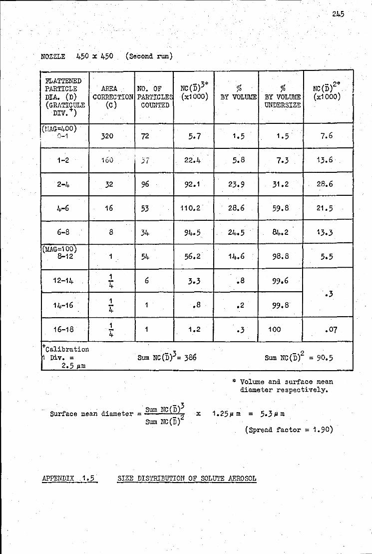
.
NOZZLE 450 x 450 . (Second run)
FLATTENED NC(i5)3* PARTICLE . AREA NO. OF
DIA. (D) CORRECTION PARTICLE~ (x1000) (GRATI~ULE (c) COUNTED
DIV. )
(FAG=400) ()-1 320 . 72 5.7
1-2 160 57 22.4
2-4 32 96 92.1
4-6 16 53 11 o. 2.
.
6-a a 34 94.5
(MAG-=1 0~) 8-12 1 54 56.2
12-14 1 6 3.3 4
14-16 1 1 .a 4
16-1a 1 1 1.2 4 +calibration
Sum NC (D )3 = 3a1) ~ Div. = 2. 5 pm
. • Sum NC(ii)3 Surface mean d~ameter = 2 x
Sum NC(D)
245
NC (D )2* % % BY VOLUME BY VOLUME (x1 000)
UNDERSIZE
1.5 1.5 7.6
5.a 7.3 13.6
23.9 31.2 28.6
2a.6 59.a . 21.5
24.5 84.2 13.3
14.6 9a.a 5.5
.a 99.6 .3
.2 99.a
.3 100 .07
Sum NC(n)2 = 90.5
.
* Volume and surface mean diameter respectively.
1.25!1 m = 5·311 m
(Spread factor= 1.90)
APPENDIX 1 • 5 SIZE DIS1'RIBUTION OF SOLUTE .ft.EROSOL
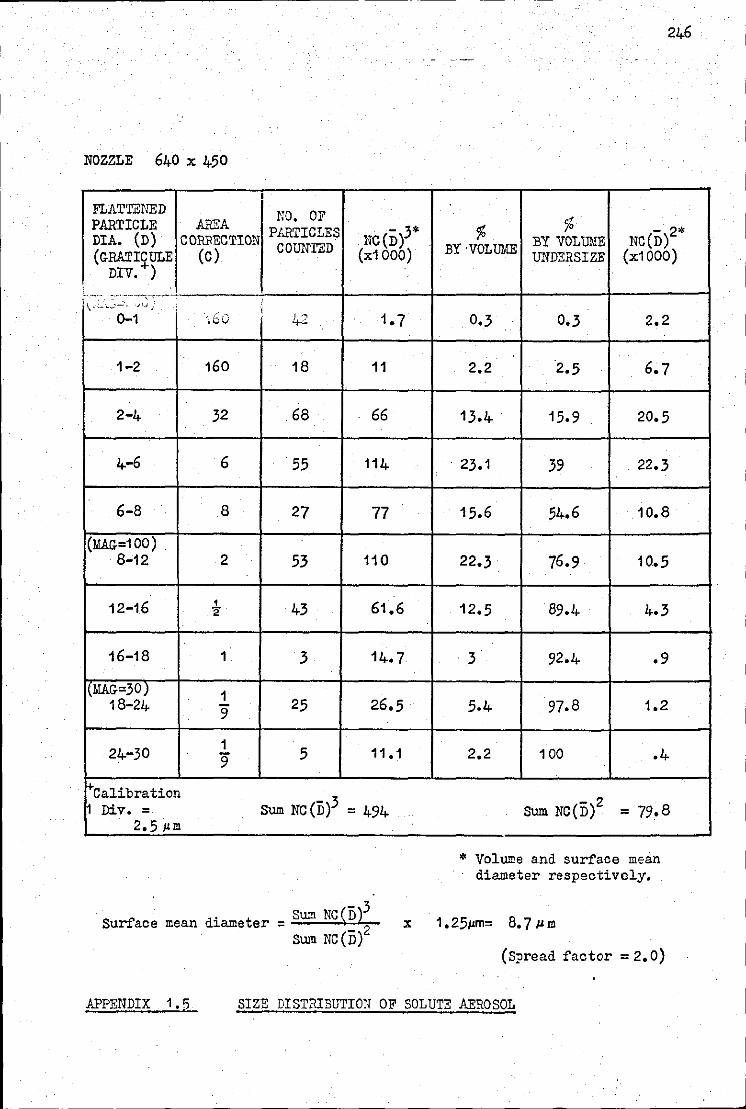
NOZZLE 640 x 450
FLAT'l'ENED PARTICLE AREA DIA. (D) CORRECTION (GRATI~ULE
DIV. ) (C)
t' -··- ·-·~· -·-·-,--,---~
\· -~~--· ~ ' 0-1 'ibO
I 1-2 160
2-4 32 .
4-6 6 .
6-8 8
(MAG=100) . 8-12 2
.
12-16 1 '2
16-18 1
I\MAG=30) 1 18-24 9
24-30 1 9
+calibration h Div. =
2. 5 I'm
I
~:o. OF PJJlTICLES NC(D)3* COUNTED (x1 000)
' I
·~ 1. 7 4-:;:.
18 11
68 66
55 114
27 77
53 110
43 61.6
3 14.7
25 26.5
5 11 .1
Sum NC(D)3 = 494
246
% % NC(D)
2* BY VOLUME BY ·VOLUME UNDERSIZE (x1000)
0.3 . 0.3 2.2
2.2 2.5 6.7
13.4 15.9 20.5
. 23.1 39 22.3
15.6 54.6 10.8
22.3 76.9 10.5
12.5 89.4 4.3
3 92.4 .9
5.4 97.8 1.2
2.2 100 .4
Sum NC(nl = 79.8
* Volume and surface mean diameter respectively.
. Sum NC~n)3 Surface mean d~ameter = 2 x 1 • 251'm= 8. 7 ll m Sum NC(D)
(Spread factor = 2. 0)
APPENDIX 1 • 5 SIZE DISTRIBUTION OF SOLUTE AEROSOL
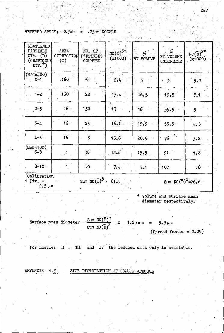
METERED SPRAY; 0.51lim x .25mm NOZZLE
FLATTENED . PARTICLE. AREA NO. OF NC(ii)3* DIA. (D) CORRECTIO!i PARTICLES (GRATI~UL:! (C) COUNTED (x1 000)
DIV. )
[fMAG=4-00) .
0-1 160 61 2.4 ! ··--------···--··-·· ....•... -·- •......
' . ' 1-2 160 22 "-.~) ,.l.;.
2-3 16 50 13
3-4 16 23 16.1
4-6 16 8 16.6
I~MAG=100) 6-8 1 36 12.6
8-10 1 10 7.4
Calibration Sum NC (ii )3 = Div. = 81.5
2,5. pm .
SUrface mean diameter = Sum NC(ii)3
· x Sum NC(ii)2
I
247
.
% % Nc(iil• BY VOLuME BY VOLUME UNDERSIZE (x1000)
3 3 3.2
16.5 19.5 8.1
.
16 35.5 5
19.9 55.5 4.5
20.5 76 3.2
15.5 . 91 1.8
9.1 100 .8
Sum NC(ii)2
=26.6
* Volume and surface mean diameter respectively.
1.25.um = 3.9pm
(Spread factor = 2,05)
For nozzles IT , m and IV the reduced data only is available.
APPENDIX 1 • 5 SIZE DISTRIBUTION OF SOLUTE AEROSOL
J
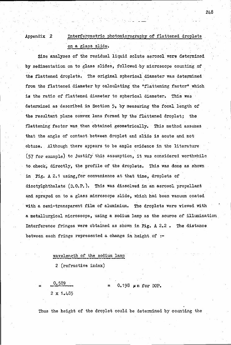
248
J.ppendix 2 Interferometric photomicrography o~ ~lattened droplets
on a glass slide~
Size analyses o~ the residual liquid solute aerosol were determined
by sedimentation on to glass slides, ~ollowed·by microscope counting of
the ~lattened droplets, The original spherical diameter was determined
from the flattened diameter by calculating the "~lattening f'actor" which
is the ratio of flattened diameter to spherical diameter. This was
determined as described in Section 5, by measuring the focal length of
the resultant plane convex lens formed by the ~lattened droplet; the
flattening factor was then obtained geometrically. This method assumes
that the angle of contact between droplet and slide is acute and not
obtuse •. Although there appears to be ample evidence in the literature
(57 for example) to justify this assumption, it was considered worthwhilo
to check, directly, the profile o~ the droplets. This was done as shown
in Fig. A 2.1 using,~or convenience at that time, droplets of
dioctylphthalate (D.O.P. ), This was dissolved in an aerosol propellant
and sprayed on to a glass microscope slide, which had been vacuum coated
with a semi-transparent film of aluminium, The droplets were viewed with
a metallurgical microscope, using a sodium lamp as the source o~ illumination
Inter~erence fringes were obtained as shown in Fig. A 2,2 • The distance
between each f'ringe represented a change in height o~ :-
=
wavelength o~ the sodium lamp
2 (refractive index)
0.589 = 0,198 p. m for OOP,
2 X 1,485
Thus the height of the droplet could be determined by coun~ing the
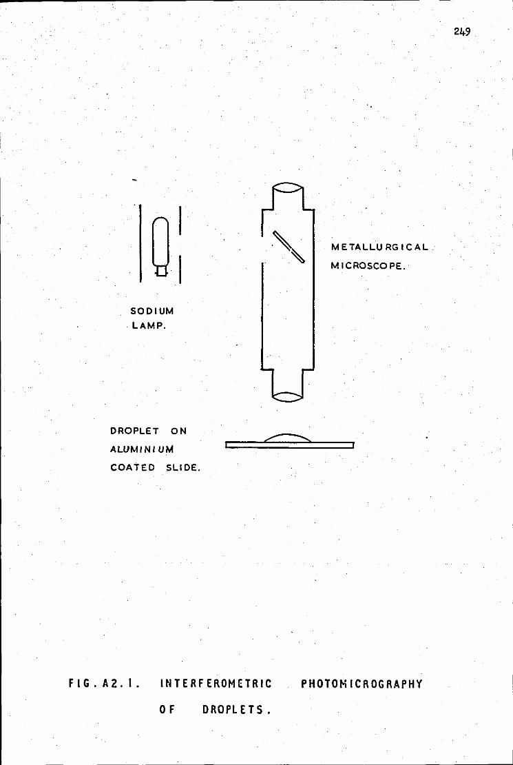
SODIUM
·LAMP.
DROPLET ON
ALUMINIUM
COATED SLIDE.
FIG.A2.1. INTERFEROMETRIC
OF DROPLETS.
METALLURGICAL.
MICROSCOPE.
PHOTOMICROGRAPHY
249
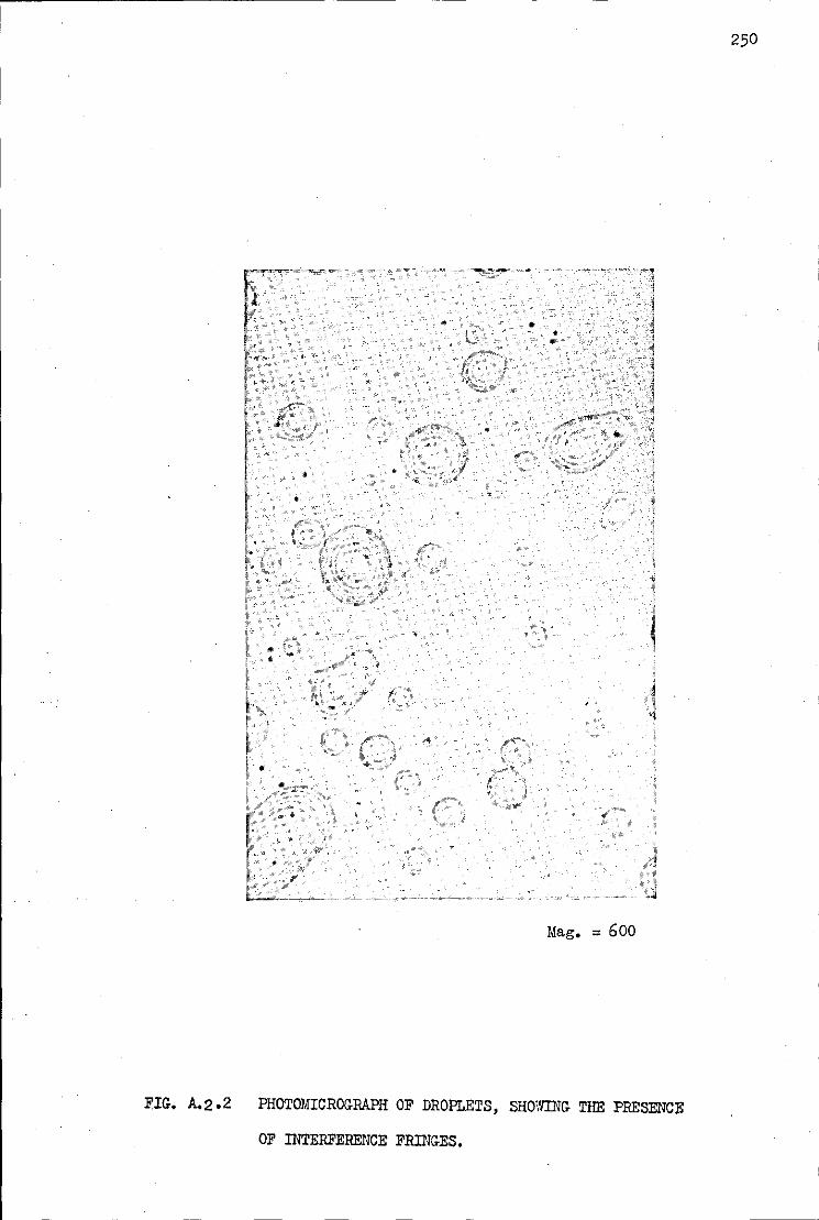
• •
•
'
Mag, = 600
PHOTOMICROGRAPH OF DROPLETS, SHOWING THE PRESENCE
OF INTERFERENCE FRINGES,
250
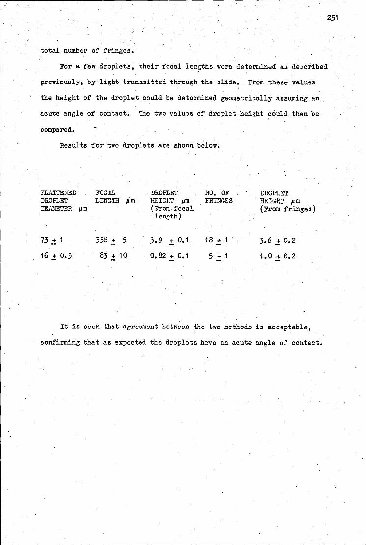
251
total number of fringes.·
For a few droplets, their focal lengths were determined as described
previously, by light transmitted through the slide. From these values
the height of the droplet could be determined geometrically assuming an
acute angle of contact. The two values of droplet height could then be
compared.
Results for two droplets are shown below.
FLATI'ENED FOCAL DROPLET NO. OF DROPLET DROPLET :LENG-TH !liD HEIG-HT pm FRING-ES HEIG-HT !liD DEAMETER pm (From focal (From fringes)
length)
73 :!:. 1 358..:!: 5 3.9 + 0.1 18 + 1 3.6.:! 0.2 .-16:!:. o.s 83:!:. 10 o. 82 :!:. 0.1 5 ..:!: 1 1.0_:!0.2
It is seen that agreement between the two methods is acceptable,
confirming that as expected the droplets have an acute angle of contact.
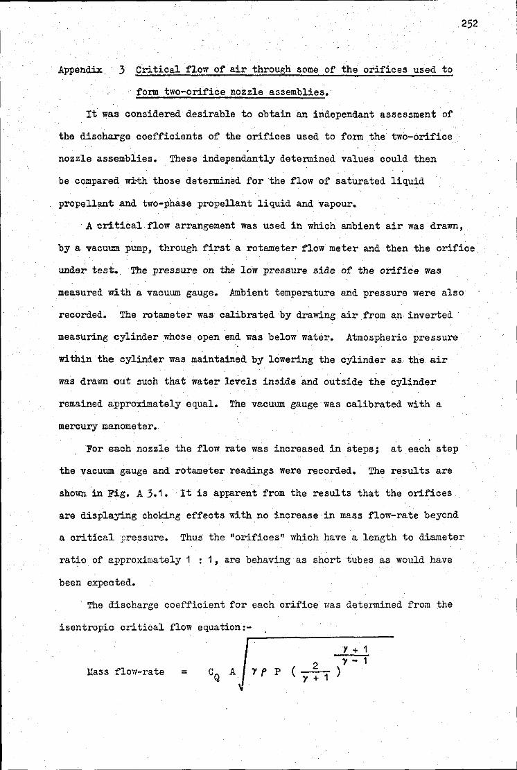
252
Appendix 3 Critical flow of' air through some of' the orif'ices used to
f'orm two-orif'ice nozzle assemblies,·
It was considered desirable to obtain an independant assessment of
the discharge coef'f'icients of' the orif'ices used to f'orm the two-orif'ice ·
nozzle assemblies, These independantly determined values could then
be compared ~th those determined f'or the f'low of' saturated li~uid
propellant and two-phase propellant li~uid and vapour.
·A critical f'low arrangement was used in which ambient air was drawn,
by a vacuum pump, through f'irst a rotameter f'low meter and then the orif'ice
under test. The pressure on the low pressure side of' the orif'ice was
measured with a vacuum gauge. Ambient temperature and pressure were also
recorded. The rotameter was calibrated by drawing air f'rom an inverted
measuring cylinder whose open end was below water, Atmospheric pressure
within the cylinder was maintained by lowering the cylinder as. the air
was drawn out such that water levels inside and outside the cylinder
remained approximately e~ual. The vacuum gauge was calibrated with a
mercury manometer.
For each nozzle the flow rate was increased in steps; at each step
the vacuum gauge and rotameter readings were recorded, The results are
shown in Fig. A 3.1. It is apparent f'rom the results that the orif'ices
are displa:ying choking effects with no increase in mass f'low-rate beyond
a critical pressure. Thus the "orifices" which have a length to diameter
ratio of approximately 1 1, are behaving as short tubes as would have
been expected,
The discharge coefficient for each orifice was determined from the
isentropic critical f'low e~uation:-~--------~------
Mass f'low-rate = G A Q
y f p 2 ( y + 1 )
y + 1 y- 1
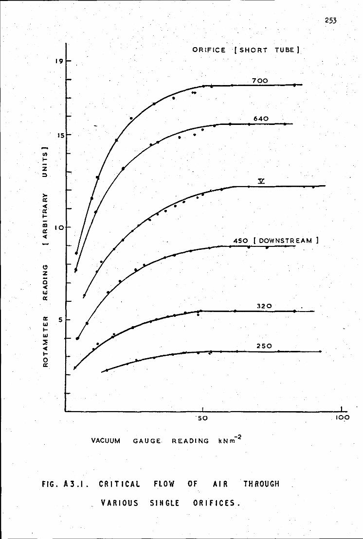
~
U)
.... -z ::1
> a: < a: .... -Ill a: <
C)
z a < Ul a:
IS
10
Cl: s Ul .... UJ
;, < .... 0 a:
VACUUM GAUGE
ORIFICE (SHORT TUBE I
•
•
0 :#
·so
READING
450
-2 kNm
700
640
(DOWNSTREAM I
320
2SO 0
FIG. A3.1. CRITICAL FLOW OF AIR THROUGH
VARIOUS SINGLE ORIFICES.
253
100
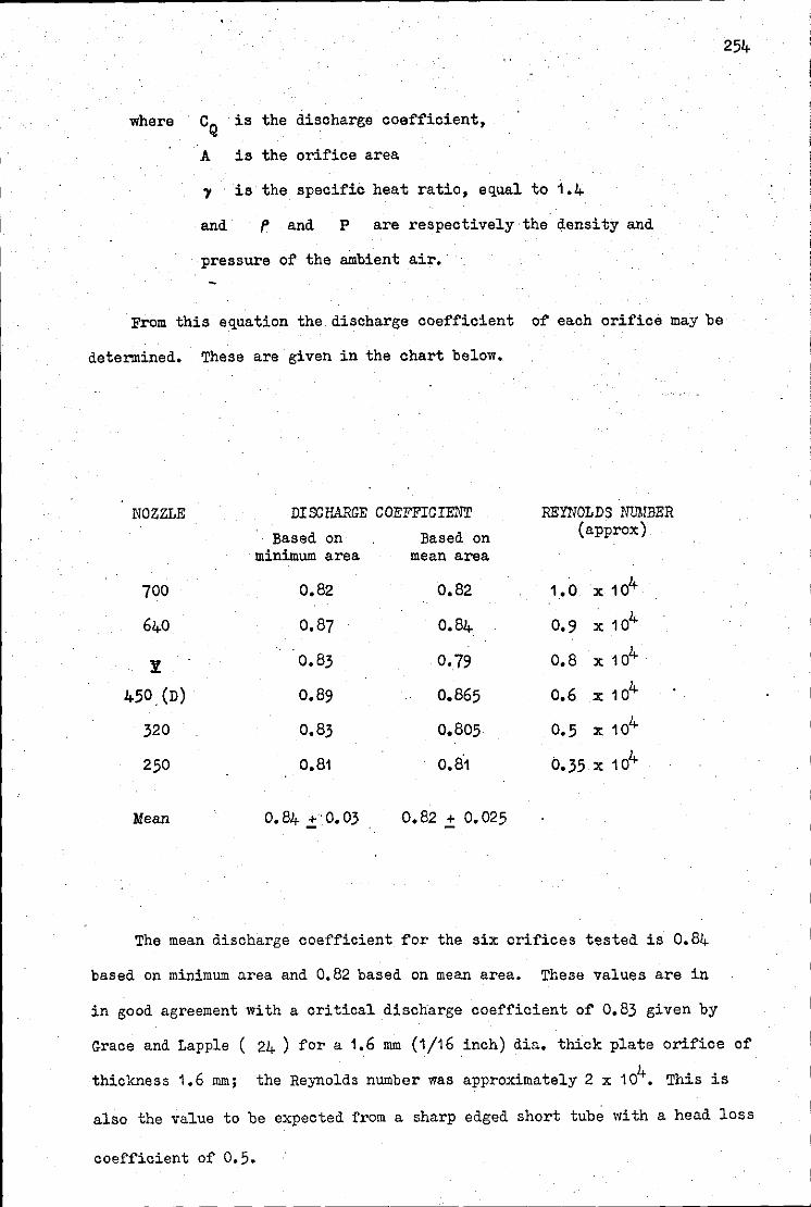
254
where CQ is the discharge coefficient,
A is the orifice area
')I is the specific heat ratio, eg_ual to 1.4
and f' and p are respectively the ij.ensity and
pressure of the ambient air.
From this eg_uation the discharge coefficient of each orifice may be
determined. These are given in the chart below.
NOZZLE DISCHARGE COEFFICIENT REYNOLDS NUMBER
Based on Based on (approx)
minimum area mean area
700 0,82 0,82 1,0 X 10⁴
640 0.87 0.84 0.9 X 10⁴
1! 0.83 0.79 0,8 X 10⁴
450 (D) 0,89 0,865 0,6 X 10⁴
320 0,83 0,805 0.5 X 10⁴
250 0,81 0.81 0,35 X 10⁴
Mean 0.84 + 0.03 0,82.:!: 0,025
The mean discharge coefficient for the six orifices tested is 0.84
based on minimum area and 0,82 based on mean area. These values are in
in good agreement with a critical discharge coefficient of 0.83 given by
Grace and Lapple ( 24) for a 1,6 mm (1/16 inch) diu. thick plate orifice of
thickness 1,6 mm; the Reynolds number was approximately 2 x 10⁴• This is
also the value to be expected from a sharp edged short tube with a head loss
coefficient of 0.5.
- --------~ ---
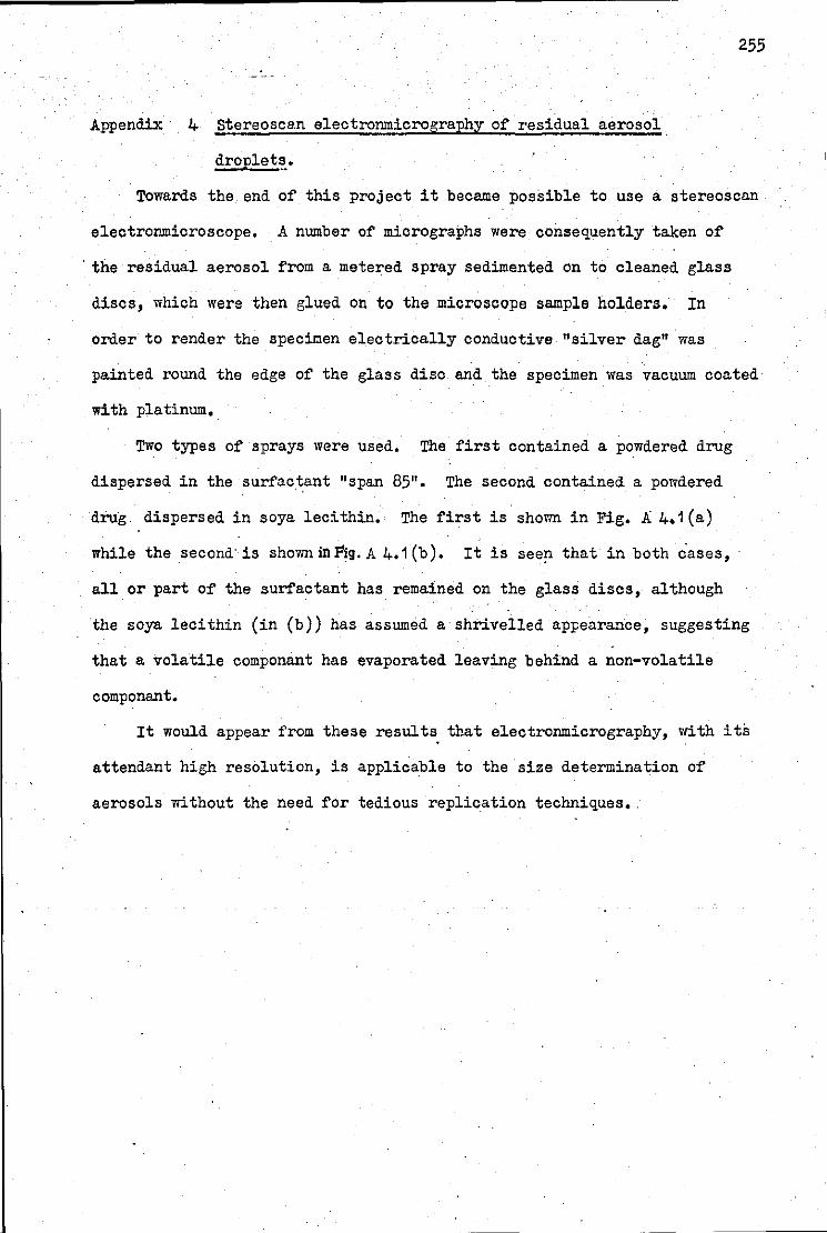
Appendix 4 Stereosca.n electronmicrography of residual aerosol
droplet~.
255
Towards the end of this project it became possible to use a stereoscan
electronmicroscope. A number of micrographs were consequently taken of
· the residual aerosol from a metered spray sedimented on to cleaned glass
discs, which were then glued on to the microscope sample holders. In
order to render the specimen electrically conductive "silver dag" was
painted round the edge of the glass disc and the specimen was vacuum coated
with platinum.
Two types of sprays were used. The first contained a powdered drug
dispersed in the surfac.tant "span 85". The second contained a powdered
drug. dispersed in soya lecithin. The first is shown in Fig. Ji. 4.1(a)
while the second· is shovm in Pig. A 4.1 (b). It is seen that in both cases,
all or part of the surfactant has remained on the glass discs, although
the soya lecithin (in (b)) has assumed a shrivelled ap];earance, suggesting
that a volatile componant has evaporated leaving behind a non-volatile
componant.
It would appear from these result~ that electronmicrography, with its
attendant high resolution, is applicable to .the size determination of
aerosols without the need for tedious replication techniques •.
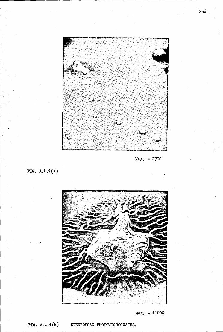
FIG. A.4.1(a)
FIG. A.4.1 (b)
Mag, = 2700
Mag. = 11000
STEREOSCAN PHOTOMICROGRAPHS.
256
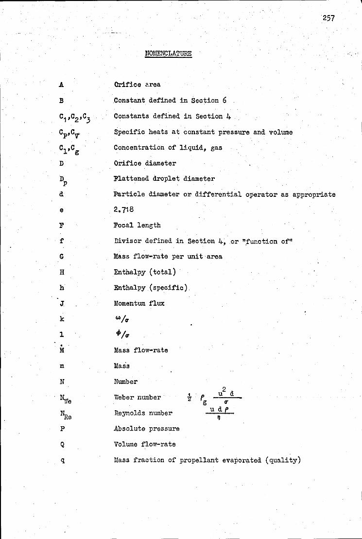
A
B
c1,c2,c3
CP,CV
c1,cg
D
e
F
f
G
H
h
J
k
1
• M
m
N
Q
q
257
lTOMENCLATURE
Orifice ~.rea
Constant defined in Section 6
Constants defined in Section 4
Specific heats at constant pressure and volume
Concentration of liquid, gas
Orifice diameter
Flattened droplet diameter
Particle diameter or differential operator as appropriate
Focal length
Divisor defined in Section 4, or ".function of"
Mass flow-rate per unit area
Enthalpy (total)
Enthalpy (specific)
Momentum flux
Mass flow-rate
Mass
Number
Weber number
Reynolds number
Absolute pressure
Volume flow-rate
Mass fraction of propellant evaporated (quality)
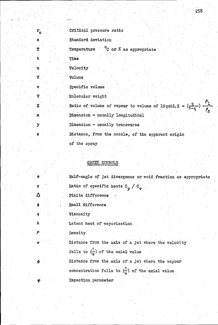
s
T
t
u
V
V
w
X
·x
y
z
a
,.
6
f'
(f
258
Critical pressure ratio
Standard deviation
Temperature
Time
Velocity
Volume
Specific volume
Molecular weight
Ratio of volume of vapour to volume of liquid.X
Dimension - usually longitudinal
= (..3-) !J_ 1-q {',
g
Dimension - usually transverse
Distance, from the nozzle, of the apparent origin
of the spray
GREEK SU.IBOLS
Half-angle of jet divergence or void fraction as appropriate
Ratio of specific heats cp I CV
Finite difference
Small difference
Viscosity
Latent heat of vaporisation
Density
Distance from the axis of a jet where the velocity
falls to c.!.) O·f the axial value e .
Distance from the axis of a jet where the vapour
concentration falls to (1) of the axial value e .
Impaction parameter
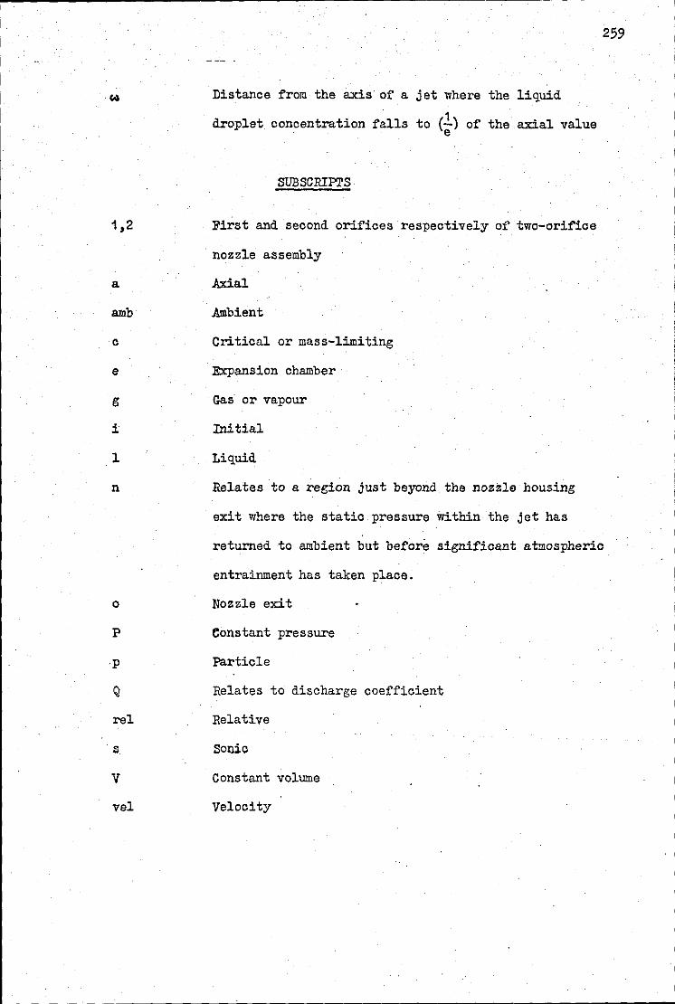
1,2
a
amb
c
e
g
i
1
n
0
p
,p
Q
rel
V
vel
Distance from the axis of a jet where the liquid
1 droplet concentration falls to (e) of the axial value
SUll SCRIPl'S
First and second orifices respectively of two-orifice
nozzle assembly
Axial
.Ambient
Critical or mass-limiting
Expansion chamber
Gas or vapour
Initial
Liquid
Relates to a region just beyond the nozzle housing
exit where the static pressure Within the jet has
259
returned to ambient but before significant atmospheric
entrainment has taken place.
Nozzle exit
Constant pressure
Particle
Relates to discharge coefficient
Relative
Sonic
Constant volume
Velocity
•
•
260
SUPERSCRIPTS
Indicates that the value is reduced to standard conditions
Mean value
u: Time average value of velocity
Denotes a dimensionless quantity
Time derivitive
BIBLIOGRAPHY
1 Benatt, F.G.S. & Eisenklam, P.
J, Inst. Fuel ~ p.309 1969
2.. Bens on, G. M. et al.
A.R.S.J. 30 p.447 1960
3 Briffa, F. E. J. & Dombrowsk:l., N.
A.I.Ch.E,J. 11(4) p.708 1966
4 British Standard Institut·e
BS 1042 "Measurement of Fluid Flow in Pipes" 1964
5 British Standard Institute
BS 3406 pt.4 "Determination of Particle Size of Powders:
Optical Microscope Method" 1963
6 Brown, R. & York, J.L.
A.I.Ch.E,J. ~ p.149 1962
7 Coull, J. & Stuart, E.B •
. "Equilibrium Thermodynamics" John Wiley & Sons Inc. 1964
8 Davies, C. N.
s. R. I. Journal p. 124 1961
9 Davies, C. N.
"Aerosol Science" Academic Press 1966
10 De Velis, J.B. et al.
J. Opt. Soc. Amer 56 p.423 1966
11 Dombrowski, N. & J.iunday, G.
Biochemical and Biological Engineering Science Vo1.2
Academic Press 1968
12 Edmonds, D,K, & Smith, R. V.
Symposium on •rwo-Phase Flow Exeter 1965
261
13 Eggins, P.L. & Jackson, D.A.
J. Appl. Physics 1 p.1894 1974
14 Fauske, H. K.
A.N.L. Report No.6633 1962
15 Fauske, H.K.
Proc. Symp. on Two-Phase Flo1v Exeter 1965
16 Fauske, H.K. & Min, A. C.
A.N.L. Report No.6667 1963
17 Finlay, I. C. & Welsh, N.
N.E.L. Report No.331 1967
18 Fourney, M.E. et al.
Rev. Sci. Insts. 40 p.205 1969
19 Fulton, R. et al.
C.S.M.A. Proc. p.51 1950
20 Goetz, A. Stevenson, H. & Preining, 0.
J. Air Pollution Control Ass. 10 p.378 1960
21 Goldschmidt, V. & Eskinazi, S.
Trans. A. S.J.I.E. J. App. Mech. 33 p. 735 1966
22· Gordon, G. D.
J. App. Phys. 30 p.1759 1959
23 Gouse, S. w. & Brown, G. A.
A. S.M.E. Paper No. 64- \'IA/F'E- 35 1964
24 Grace, H.P. & Lapple, C.E.
Trans. A. S.M.E. 73 p.639 1951
25 Green, H.L. & Lane, ·:r.R.
262
"Particulate Clouds: Dusts,Smokes and Mists" E. & F.N. Spon Ltd.
1951
26 Groeneweg, s. et al.
Brit. J. App. Phys. 18 p.1317 1967
I
27 Haas, F.C.
A.I.Ch.E.J. 10 p.920 1964
28 Henry, R.E. et al.
Proc. Int, Conf, "Research into Concurrent Gas-Liquid Flow"
Univ. of ;1aterloo Sept. 1968
29 Hinze, J.O.
A.I.Ch.E.J • .!. (3) p,289 1955
30 Imperial Smelting Corporation
"Isceon" 1962
31 Jngebo, R. D,
A.R.S,J. ~. p.540 1961
32 Ingebo, R. D.
Chem. Eng. Prog. 58 p.74 1962
33 JO.ingebiel, W. J. & Moul ton, R. \'l,
A,I.Ch,E.J, .!.Z(2) . p.383 1971
34 Laats, M.K.
Trans, from Inzhinerno Fizicheskii Zhurnal 10 p.11 1966
3 5 Landahl, H. D.
Bull, Math. Biophys, 12 p.43 1950.
36 Lane, \'1, R.
Ind. Eng. Chem. 43 p.1312 1951 -. 37 Lange, H.
"Nonionic Surfactants" Ed. !.!, J. Schick !J. Dekker 1967
38 Lefebvre, !.!. & Tregan
Parf, Cosm. Sav. 1 p.276 1964
39 May, K. R.
J. Sci. Inst. 22 p.187 1945
40 Mayer, E.··:;. & H.anz ·::.E.
263
Encyclopeadia of Chemical Technology Ed. R.Kirk & D.F.Otbner
Inter Science Encyclopeadia Inc. New York 1960
41 Metals Research Ltd,
The Quantimet-Image Analysing Computer
42 Mi tchell, R. I.
Amer. Rev. Reap. Dis, 82 p.627 1960
43 L!itchell, R. I. & Filcher, J.M.
Ind.. Eng. Chem • .2.2. p.1039 1959
44 Moody, F.J.
Trails. A.S.J.I.E. J, Heat Transfer p.37 Aug.1969
45 Moroney, M.J.
Facts From Figures Penguin Books Ltd. 1969
46 Nukiyama, S. & Tanasawa, Y •.
Trans. Soc. Mech. Eng. Japan ,!!; p,186 1938
47 Orr, C.
"Particula te Technology" McMillan 1966
48 Oxford Industrial Research & Development
Packaeing Review p.24 Nov. 1966
49 Pai, C. Y. F.
"Fluid Dynamics of Jets" Van Nostrand 1954
50 Pasqua, P.F.
Refrig. Eng. 61 p,1084 1953
51 Polli, G. P. et al.
J. Pharm. Sci. 58 p.484 1969
52 Ramshaw, c.
J. Inst. Fuel 41 p.288 1968
53 Lord Rayleie;h
Proc. London. Math. Soc. 10 1878
54 Reichardt, H.
Z Anr,ew l:.ath. & 1lech. 21 p.257 1941
55 Royco Inst. Inc.
"The Royco :Aerosol Fhotometer"
264
56 Sawyer, K. & .Val ton, ·iT. H.
J. Sci. Inats 27 p.272 1950
57 Schonauer, G.
Staub-Reinhalt, Luf't 27 p. 7 1967
58 Schonauer, G.
Staub-Reinhalt, Luf't 27 p.27 1967
59 Smith, R. V.
N. B. S. Tech Note No.179 1963
60 Soo, S.L.
Fluid Dynamics of Mul tiphase Systems" Blaisdell Publishing
eo. 1967
61 Stuart, M. C. & Yarnall, D.R.
Mech, Eng, 58 p.479 1936
62 Stuart, M.C. & Yarnall, D.R.
Trans. A. s. M. E. 66 p. 387 1944
63 Tangren, R.F. et al.
J. App Phys. 20 (7) p.637 1949
64 Technical Operations Inc.
"Laser Hologram Camera System"
65 Thompson, B.J. et al.
Applied Optics 6 p.519 1967
66 Tovmsend, A.A.
265
"The Structure of Turbulent Shear Flow" Cambridge Univ. Press
67 Tsetlin, V.l•!.
The Soviet Chemical Industry 8 p.70 1969
68 Van Ligten, R.F.
"Holographic Microscopes and &nall Particles"
1956
AI:lerican Optic::tl Corr. Research Group Report, Framigham Centre,ltass.
69 Ward, J, & Thompson B.J.
J. Opt. Soc. Am • .21P· 275 1967
70 Weber, c.
Z .Angew Math, Mech, 11 p.136 1931
71 V11li tby, K. T. &. Clark W. E.
Tellus 18 p.573 1965
72 Whitby, K.T.
266
Progress Report No, AP 00480-2 Univ, of Minnisota Aug. 1967
73 Wilke 1 C. R.
J, Chem. Phys, 18 p. 517 1950
74 York, J.L.
J, Soc. Cos, Chem. 1 p,204 1956
75 York, J,L, & Stubbs, H.E.
Trans, A.S.M.E. 74 p.1157 1952
76 Young, E. G.
C.S.M.A. Proceedings p.42 1950