Factorization of noncommutative polynomials with applications · Factorization of noncommutative...
61
Factorization of noncommutative polynomials with applications Jahrestagung DFG SFB-TRR 195 Viktor Levandovskyy Lehrstuhl D f¨ ur Mathematik RWTH Aachen University, Germany Project II.6, PI Eva Zerz 26.09.2017 1 / 40
Transcript of Factorization of noncommutative polynomials with applications · Factorization of noncommutative...

Factorization of noncommutative polynomialswith applications
Jahrestagung DFG SFB-TRR 195
Viktor Levandovskyy
Lehrstuhl D fur MathematikRWTH Aachen University, Germany
Project II.6, PI Eva Zerz
26.09.2017
1 / 40

Plan of Attack
Non-Commutative Finite Factorization Domains
A General Non-Commutative Factorization Algorithm
Non-Commutative Factorized Grobner Bases
Conclusion and Future Work
2 / 40

Factorization Properties of Integral DomainsLet K be a field. Most of us usually deal with two kinds ofintegral domains (commonly assumed to be commutative rings;Bourbaki call them factorial rings):
I UFDs (unique factorization domains) incl. regular local rings,
I non-UFDs like Z[i√
5], where 6 = 2 · 3 = (1 + i√
5)(1− i√
5)or K[x , y , z ]/〈xy − z2〉, where [z ] · [z ] = [x ] · [y ].
Factorization properties of integral domains: see, for instance
I Anderson, D., Anderson, D., and Zafrullah, M. (1990).Factorization in integral domains. Journal of pure and appliedalgebra, 69(1):1–19.
I Anderson, D. and Mullins, B. (1996). Finite factorizationdomains. Proceedings of the AMS, 124(2):389–396.
I Anderson, D. (1997). Factorization in integral domains,volume 189, CRC Press.
Weakening the UFD property: FFD := finite factorization domain.
3 / 40

Factorization Properties of Integral DomainsLet K be a field. Most of us usually deal with two kinds ofintegral domains (commonly assumed to be commutative rings;Bourbaki call them factorial rings):
I UFDs (unique factorization domains) incl. regular local rings,
I non-UFDs like Z[i√
5], where 6 = 2 · 3 = (1 + i√
5)(1− i√
5)or K[x , y , z ]/〈xy − z2〉, where [z ] · [z ] = [x ] · [y ].
Factorization properties of integral domains: see, for instance
I Anderson, D., Anderson, D., and Zafrullah, M. (1990).Factorization in integral domains. Journal of pure and appliedalgebra, 69(1):1–19.
I Anderson, D. and Mullins, B. (1996). Finite factorizationdomains. Proceedings of the AMS, 124(2):389–396.
I Anderson, D. (1997). Factorization in integral domains,volume 189, CRC Press.
Weakening the UFD property: FFD := finite factorization domain.3 / 40

What has been done for Non-Commutative Domains?
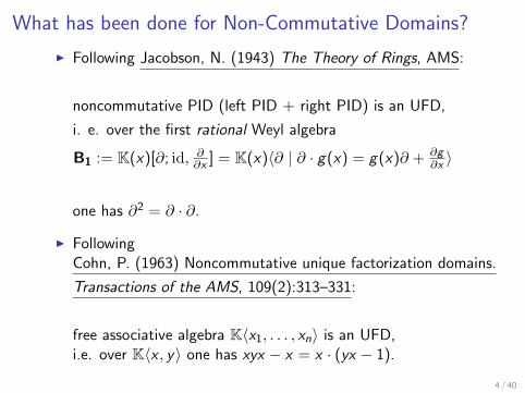
I Following Jacobson, N. (1943) The Theory of Rings, AMS:
noncommutative PID (left PID + right PID) is an UFD,
i. e. over the first rational Weyl algebra
B1 := K(x)[∂; id, ∂∂x ] = K(x)〈∂ | ∂ · g(x) = g(x)∂ + ∂g∂x 〉
one has ∂2 = ∂ · ∂.
I FollowingCohn, P. (1963) Noncommutative unique factorization domains.
Transactions of the AMS, 109(2):313–331:
free associative algebra K〈x1, . . . , xn〉 is an UFD,i.e. over K〈x , y〉 one has xyx − x = x · (yx − 1).
4 / 40
What has been done for Non-Commutative Domains?
I Following Jacobson, N. (1943) The Theory of Rings, AMS:
noncommutative PID (left PID + right PID) is an UFD,
i. e. over the first rational Weyl algebra
B1 := K(x)[∂; id, ∂∂x ] = K(x)〈∂ | ∂ · g(x) = g(x)∂ + ∂g∂x 〉
one has ∂2 = ∂ · ∂.
I FollowingCohn, P. (1963) Noncommutative unique factorization domains.
Transactions of the AMS, 109(2):313–331:
free associative algebra K〈x1, . . . , xn〉 is an UFD,i.e. over K〈x , y〉 one has xyx − x = x · (yx − 1).
4 / 40

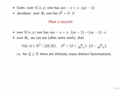
I Cohn: over K〈x , y〉 one has xyx − x = x · (yx − 1)
I Jacobson: over B1 one has ∂2 = ∂ · ∂
Wait a second!
I over K〈x , y〉 one has xyx − x = x · (yx − 1) = (xy − 1) · xI over B1, we can see (after some work), that
∀(b, c) ∈ K2 \ {(0, 0)}, ∂2 = (∂ + bbx−c ) · (∂ − b
bx−c ),
i.e. for Q ⊆ K there are infinitely many distinct factorizations.
I in both cases Bell, Heinle and L. proved, that these are allfactorizations.
Where’s the mistake?
5 / 40

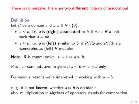
There is no mistake: there are two different notions of association!
DefinitionLet R be a domain and a, b ∈ R \ {0}.
I a ∼ b, i.e. a is (right) associated to b, if ∃u ∈ R a unit,such that a = ub.
I a ≈ b, i.e. a is (left) similar to b, if R/Ra and R/Rb areisomorphic as (left) R-modules.
Note: R is commutative: a ∼ b ⇔ a ≈ b.
R is non-commutative: in general a ∼ b ⇒ a ≈ b only.
For various reasons we’re interested in working with a ∼ b,
e. g. it is not known, whether a ≈ b is decidablealso, multiplication in algebras of operators stands for composition.
6 / 40

Example
Consider a polynomial from (Tsai, 2000, Example 5.7) in the firstpolynomial Weyl algebra A1 = K〈x , ∂ | ∂ · x = x∂ + 1〉
p =(x6 + 2x4 − 3x2)∂2 − (4x5 − 4x4 − 12x2 − 12x)∂
+ (6x4 − 12x3 − 6x2 − 24x − 12),
which has two different factorizations w.r.t. ∼:
p =(x4∂ − x3∂ − 3x3 + 3x2∂ + 6x2 − 3x∂ − 3x + 12)·(x2∂ + x∂ − 3x − 1)
=(x4∂ + x3∂ − 4x3 + 3x2∂ − 3x2 + 3x∂ − 6x − 3)·(x2∂ − x∂ − 2x + 4)
However, w.r.t. ≈ these two factorizations are equivalent.
7 / 40

Some motivating applications
Suppose, that we can compute factorizations in an FFD R.
Partial module decomposition.Suppose, that f ∈ R \ {0} has factorizations f = gihi , i ∈ I ,|I | <∞ and gi , hi are non-units, not nec. irreducible. Then for aleft ideal L ⊂ R we have L + Rf ⊆
⋂i∈I (L + Rhi ) and
R
L + Rf→ R⋂
i∈I (L + Rhi )→ 0.
Moreover, if L + Rhi + Rhj = R for all i 6= j , then
R⋂i∈I (L + Rhi )
∼=⊕i∈I
R
(L + Rhi ).
The “factorizing Grobner basis” technique (details below) takes aleft ideal L ⊂ R and delivers a collection of left ideals {Bi} suchthat L ⊆ ∩Bi .
8 / 40

Some motivating applications
Partial closure with respect to an Ore set
Let S be a multiplicatively closed Ore subset of a domain R.Given a left ideal L ⊂ R, the S-closure of L is the left ideal
LS = {r ∈ R | ∃s ∈ S : s · r ∈ L} ⊂ R,
also known as the contraction of S−1L ⊂ S−1R to R.
Algorithms for the computation of LS are known only for severalcases, in general it is very complicated.
Approximate LS :if f ∈ L has factorizations of the form f = si · gi with si ∈ S ,then gi ∈ LS follows.
9 / 40

Non-CommutativeFinite Factorization Domains
10 / 40

Definitions of finite factorization domains
Definition (Commutative FFD, cf. (Anderson et al., 1990))
Let R be a (commutative) integral domain. Then R is an FFD, ifeach nonzero non-unit of R has only a finite number ofnon-associate divisors and hence, only a finite number offactorizations up to order and associates.
Bell, J. P., Heinle, A., and Levandovskyy, V. (2017).On noncommutative finite factorization domains, Trans. AMS, 369.
Definition (Non-Commutative FFD, cf. (Bell-Heinle-L. 2017))
Let A be a (not necessarily commutative) domain. We say that Ais an FFD, if every nonzero, non-unit element of A has at least onefactorization into irreducible elements and there are at mostfinitely many distinct factorizations into irreducible elements up tomultiplication of the irreducible factors by central units in A.
11 / 40

Finite Factorization Theorems
Theorem (Bell-Heinle-L. 2017)
Let K be an algebraically closed field and let A be a K-algebra.If there exists a finite-dimensional filtration {Vn : n ∈ N} on A suchthat the associated graded algebra B = grV (A) is a (notnecessarily commutative) domain over K, then A is a finitefactorization domain over K.
Theorem (Bell-Heinle-L. 2017)
Let K be a field and let A be a K-algebra.If there exists a finite-dimensional filtration {Vn : n ∈ N} on A suchthat the associated graded algebra B = grV (A) has the propertythat B ⊗K K is a (not necessarily commutative) domain, then A isa finite factorization domain.
12 / 40

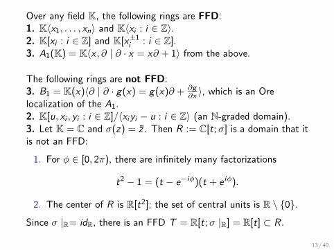
Over any field K, the following rings are FFD:1. K〈x1, . . . , xn〉 and K〈xi : i ∈ Z〉.2. K[xi : i ∈ Z] and K[x±1
i : i ∈ Z].3. A1(K) = K〈x , ∂ | ∂ · x = x∂ + 1〉 from the above.
The following rings are not FFD:3. B1 = K(x)〈∂ | ∂ · g(x) = g(x)∂ + ∂g
∂x 〉, which is an Orelocalization of the A1.2. K[u, xi , yi : i ∈ Z]/〈xiyi − u : i ∈ Z〉 (an N-graded domain).3. Let K = C and σ(z) = z . Then R := C[t;σ] is a domain that itis not an FFD:
1. For φ ∈ [0, 2π), there are infinitely many factorizations
t2 − 1 = (t − e−iφ)(t + e iφ).
2. The center of R is R[t2]; the set of central units is R \ {0}.
Since σ |R= idR, there is an FFD T = R[t;σ |R] = R[t] ⊂ R.
13 / 40

The meaning of the stated TheoremsIn a K-algebra A, satisfying the conditions of one of the Theorems,
I let a ∈ A belong to Vn with n minimal with this property
I compute all factorizations of gr(a) ∈ grV (A) = B into twofactors (B is a graded algebra with fin.-dim. graded parts)
I for every such factorization gr(a) = b1 ·b2, bi ∈ Vd(i)/Vd(i)−1
• set up an Ansatz of unknown coefficients from Kfor the lower order terms of ai = bi + Vd(i)−1,s. t. a = a1 · a2, ai ∈ Vd(i)
• obtain a commutative system of polynomial equations,which is apriori 0-dimensional by the Theorems above
• obtain at most finitely many solutions for ai via solving
Due to Theorems above, this natural Ansatz is now provided withthe proof of termination.
Hence there is an algorithm, returning all factorizations of a.14 / 40

G -Algebras
DefinitionFor n ∈ N and 1 ≤ i < j ≤ n consider the units cij ∈ K∗ andpolynomials dij ∈ K[x1, . . . , xn]. Suppose, that there exists amonomial total well-ordering ≺ on K[x1, . . . , xn], such that for any1 ≤ i < j ≤ n either dij = 0 or the leading monomial of dij issmaller than xixj with respect to ≺. The K-algebra
A := K〈x1, . . . , xn | {xjxi = cijxixj + dij : 1 ≤ i < j ≤ n}〉
is called a G -algebra, if {xα11 · . . . · xαn
n : αi ∈ N0} is a K-basis of A.
Remark
I “G -algebra” is also known as “an algebra of solvable type”and “a Poincare–Birkhoff–Witt (PBW) algebra”,
I A is a Noetherian domain with nice Grobner bases theory.
15 / 40
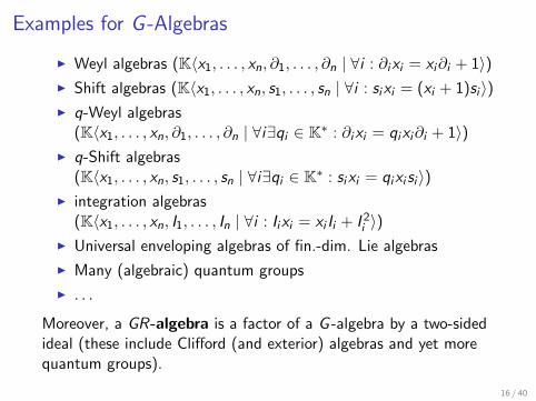
Examples for G -Algebras
I Weyl algebras (K〈x1, . . . , xn, ∂1, . . . , ∂n | ∀i : ∂ixi = xi∂i + 1〉)I Shift algebras (K〈x1, . . . , xn, s1, . . . , sn | ∀i : sixi = (xi + 1)si 〉)I q-Weyl algebras
(K〈x1, . . . , xn, ∂1, . . . , ∂n | ∀i∃qi ∈ K∗ : ∂ixi = qixi∂i + 1〉)I q-Shift algebras
(K〈x1, . . . , xn, s1, . . . , sn | ∀i∃qi ∈ K∗ : sixi = qixi si 〉)I integration algebras
(K〈x1, . . . , xn, I1, . . . , In | ∀i : Iixi = xi Ii + I 2i 〉)
I Universal enveloping algebras of fin.-dim. Lie algebras
I Many (algebraic) quantum groups
I . . .
Moreover, a GR-algebra is a factor of a G -algebra by a two-sidedideal (these include Clifford (and exterior) algebras and yet morequantum groups).
16 / 40

All G -Algebras are FFD + Complexity
Theorem (Bell-Heinle-L. 2017)
Let K be a field. Then G -algebras over K and their subalgebrasare finite factorization domains.
Lemma (Heinle-L. 2017b)
Let A be a G -algebra with K-basis {xα11 · . . . · xαn
n : α ∈ Nn0},
g ∈ A, and let d ∈ N be the total degree of g . Furthermore, letlm(g) = xα1
1 · . . . · xαnn for some α ∈ Nn
0. Then the complexity offinding all factorizations of g is of order
O
((d
α1, . . . , αn
)· (d − 1) · 2n+1 · 2(d+n−1
n ))
G - and GR-algebras are supported in Singular:Plural. Thefactorization is implemented and it is fast. It solves the problem
Calculate one/some/all factorizations of a polynomialin a GR-algebra without zero divisors over a computable field
An implementation in CAS REDUCE exists since a long time.
17 / 40

”Some” factorizationsRecall: for a mult. closed Ore set S ⊂ R and a left ideal L ⊂ R
LS = {r ∈ R | ∃s ∈ S : s · r ∈ L} ⊂ R.
Example (Special function: Legendre polynomials)
K〈n, sn | snn = nsn + sn〉 ⊗K K〈x , ∂x | ∂xx = x∂x + 1〉 is thealgebra of differential and shift operators. For char K = 0,Legendre polynomials are annihilated by two irreducible operators:
I Legendre’s P = (x2 − 1)∂2x + 2x∂x − n(1 + n)
I Bonnet’s Q = (n + 2)s2n − (2n + 3)xsn + n + 1
Consider S = K[x , n] \ {0} and the left ideal L = 〈P,Q〉. We find
(n+ 1) · (sn∂x−x∂x−n−1), (x2−1) · ((s2n−2xsn + 1) ·∂x− sn) ∈ L,
hence sn∂x − x∂x − n − 1 ∈ LS and (s2n − 2xsn + 1) · ∂x − sn ∈ LS .
Conjecture: LS = 〈P,Q, sn∂x − x∂x − n − 1〉.
18 / 40

”Some” factorizationsRecall: for a mult. closed Ore set S ⊂ R and a left ideal L ⊂ R
LS = {r ∈ R | ∃s ∈ S : s · r ∈ L} ⊂ R.
Example (Special function: Legendre polynomials)
K〈n, sn | snn = nsn + sn〉 ⊗K K〈x , ∂x | ∂xx = x∂x + 1〉 is thealgebra of differential and shift operators. For char K = 0,Legendre polynomials are annihilated by two irreducible operators:
I Legendre’s P = (x2 − 1)∂2x + 2x∂x − n(1 + n)
I Bonnet’s Q = (n + 2)s2n − (2n + 3)xsn + n + 1
Consider S = K[x , n] \ {0} and the left ideal L = 〈P,Q〉. We find
(n+ 1) · (sn∂x−x∂x−n−1), (x2−1) · ((s2n−2xsn + 1) ·∂x− sn) ∈ L,
hence sn∂x − x∂x − n − 1 ∈ LS and (s2n − 2xsn + 1) · ∂x − sn ∈ LS .
Conjecture: LS = 〈P,Q, sn∂x − x∂x − n − 1〉.18 / 40

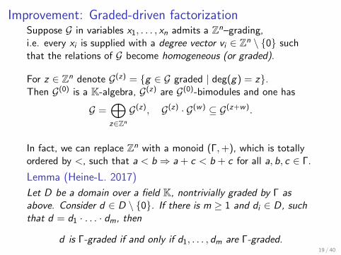
Improvement: Graded-driven factorizationSuppose G in variables x1, . . . , xn admits a Zn–grading,i.e. every xi is supplied with a degree vector vi ∈ Zn \ {0} suchthat the relations of G become homogeneous (or graded).
For z ∈ Zn denote G(z) = {g ∈ G graded | deg(g) = z}.Then G(0) is a K-algebra, G(z) are G(0)-bimodules and one has
G =⊕z∈Zn
G(z), G(z) · G(w) ⊆ G(z+w).
In fact, we can replace Zn with a monoid (Γ,+), which is totallyordered by <, such that a < b ⇒ a + c < b + c for all a, b, c ∈ Γ.
Lemma (Heine-L. 2017)
Let D be a domain over a field K, nontrivially graded by Γ asabove. Consider d ∈ D \ {0}. If there is m ≥ 1 and di ∈ D, suchthat d = d1 · . . . · dm, then
d is Γ-graded if and only if d1, . . . , dm are Γ-graded.
19 / 40
Improvement: Graded-driven factorizationSuppose G in variables x1, . . . , xn admits a Zn–grading,i.e. every xi is supplied with a degree vector vi ∈ Zn \ {0} suchthat the relations of G become homogeneous (or graded).
For z ∈ Zn denote G(z) = {g ∈ G graded | deg(g) = z}.Then G(0) is a K-algebra, G(z) are G(0)-bimodules and one has
G =⊕z∈Zn
G(z), G(z) · G(w) ⊆ G(z+w).
In fact, we can replace Zn with a monoid (Γ,+), which is totallyordered by <, such that a < b ⇒ a + c < b + c for all a, b, c ∈ Γ.
Lemma (Heine-L. 2017)
Let D be a domain over a field K, nontrivially graded by Γ asabove. Consider d ∈ D \ {0}. If there is m ≥ 1 and di ∈ D, suchthat d = d1 · . . . · dm, then
d is Γ-graded if and only if d1, . . . , dm are Γ-graded.19 / 40

Example: Zn–grading on n-th Weyl algebra
An = K〈x1, . . . , xn, ∂1, . . . , ∂n | {∂jxj = xi∂j + δij}〉.Zn-grading: deg xi = −ei , deg ∂i = ei . Then θi = xi∂i has deg 0.
Facts:
I A(0)n∼= K[θ1, . . . , θn] since xmi ∂
mi =
∏mj=0(θi − j).
I Moreover, xi and ∂i act on g(θ) ∈ K[θ] by shifting
g(θ)∂mi = ∂mi g(. . . , θi−m, . . .), g(θ)xmi = xmi g(. . . , θi+m, . . .).
I A(z)n is a K[θ]-bimodule, generated by xu1
1 · · · xunn · ∂w11 · · · ∂wn
n ,
ui :=
{−zi , if zi ≤ 0,
0, otherwise,, wi :=
{0, if zi ≤ 0,
zi , otherwise.
I θi and θi + 1 for 1 ≤ i ≤ n are the only irreducible monicpolynomials in K[θ], that are reducible in An.
20 / 40

If a grading by Γ fulfills the following properties:
1. K ⊆ G(0) is an FFD with “cheap” factorization (preferably acommutative domain, even an UFD)
2. The irreducible elements in G(0) which are reducible in G canbe identified and factorized easily (preferably, there are finitelymany monic polynomials of such type).
3. G(z) is a finitely generated (preferably cyclic, i.e. generated byone element) G(0)-bimodule,
then one can use the novel Graded-driven factorization method.
21 / 40

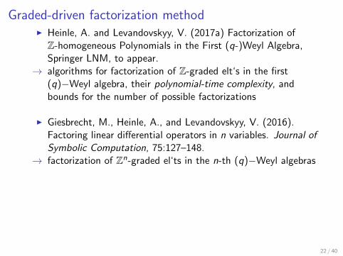
Graded-driven factorization methodI Heinle, A. and Levandovskyy, V. (2017a) Factorization of
Z-homogeneous Polynomials in the First (q-)Weyl Algebra,Springer LNM, to appear.
→ algorithms for factorization of Z-graded elt‘s in the first(q)−Weyl algebra, their polynomial-time complexity, andbounds for the number of possible factorizations
I Giesbrecht, M., Heinle, A., and Levandovskyy, V. (2016).Factoring linear differential operators in n variables. Journal ofSymbolic Computation, 75:127–148.
→ factorization of Zn-graded el‘ts in the n-th (q)−Weyl algebras
I Heinle, A. and Levandovskyy, V. (2017b). A FactorizationAlgorithm for G -Algebras and its Applications. Journal ofSymbolic Computation, in press, avail. online
→ factorization for G -algebras, graded-driven one for Zn-gradedG -algebras, factorized Grobner algorithm, complexity.
22 / 40
Some Bounds
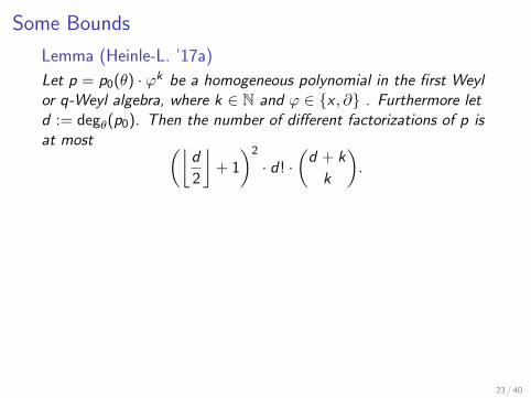
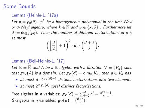
Lemma (Heinle-L. ’17a)
Let p = p0(θ) · ϕk be a homogeneous polynomial in the first Weylor q-Weyl algebra, where k ∈ N and ϕ ∈ {x , ∂} . Furthermore letd := degθ(p0). Then the number of different factorizations of p isat most (⌊
d
2
⌋+ 1
)2
· d! ·(d + k
k
).
Lemma (Bell-Heinle-L. ’17)
Let K = K and A be a K-algebra with a filtration V = {Vd} suchthat grV (A) is a domain. Let gV (d) = dimK Vd , then a ∈ Vd has
I at most d · 4gV (d)−1 distinct factorizations into two elements
I at most 2d ·gV (d) total distinct factorizations.
Free algebra in n variables: gV (d) =∑d
i=0 ni = nd+1−1
n−1 .
G -algebra in n variables: gV (d) =(d+n
n
).
23 / 40
Some Bounds
Lemma (Heinle-L. ’17a)
Let p = p0(θ) · ϕk be a homogeneous polynomial in the first Weylor q-Weyl algebra, where k ∈ N and ϕ ∈ {x , ∂} . Furthermore letd := degθ(p0). Then the number of different factorizations of p isat most (⌊
d
2
⌋+ 1
)2
· d! ·(d + k
k
).
Lemma (Bell-Heinle-L. ’17)
Let K = K and A be a K-algebra with a filtration V = {Vd} suchthat grV (A) is a domain. Let gV (d) = dimK Vd , then a ∈ Vd has
I at most d · 4gV (d)−1 distinct factorizations into two elements
I at most 2d ·gV (d) total distinct factorizations.
Free algebra in n variables: gV (d) =∑d
i=0 ni = nd+1−1
n−1 .
G -algebra in n variables: gV (d) =(d+n
n
).
23 / 40

Example
At first, we rewrite the input polynomial into its Z2-graded parts:
h = θ1(θ1 + 4)x1∂22 [−1, 2]
+ (θ1(θ1 − 1)θ2 + 8θ1θ2 + θ1 + 12θ2)x1∂2 [−1, 1]
+ (θ1(θ1 − 1)θ2 + θ21 − θ1 + 4θ1θ2 + 2θ1 + 7θ2)x1 [−1, 0]
+ (θ1(θ1 − 1)θ2 + 5θ1θ2 + 3θ2 + 1)x1x2 [−1,−1]
+ (θ1 + 1)x1x22 [−1,−2].
At second, consider one pair of factorizations of
I the highest graded part h[−1,2] = θ1∂2 · (θ1 + 4)x1∂2
I the lowest graded part h[−1,−2] = x2 · (θ1 + 1)x1x2
We look for p, q such that h = p · q, where p = θ1∂2 + . . .+ x2
and q = (θ1 + 4)x1∂2 + . . .+ (θ1 + 1)x1x2.
24 / 40
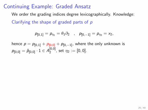
Continuing Example: Graded Ansatz
We order the grading indices degree lexicographically. Knowledge:
Clarifying the shape of graded parts of p
p[0,1] = pη1 = θ1∂2 , p[0,−1] = pη3 = x2,
hence p = p[0,1] + p[0,0] + p[0,−1], where the only unknown is
p[0,0] = p[0,0] · 1 ∈ A[0,0]2 , set η2 := [0, 0].
Clarifying the shape of graded parts of q
q[−1,1] = qµ1 = (θ1 + 4)x1∂2 , q[−1,−1] = qµ3 = (θ1 + 1)x1x2,
thus q = q[−1,1] + q[−1,0] + q[−1,−1], where the only unknown is
q[−1,0] = q[−1,0] · x1 ∈ A[−1,0]2 , set µ2 := [−1, 0].
Therefore the unknowns are commutative polynomials p[0,0] andq[−1,0] from K[θ1, θ2].
25 / 40

Continuing Example: Finiteness and Bounds
Lemma (Giesbrecht-Heine-L.’16)
For fixed h, pη1 , qµ1 , pηk and qµl ∈ An such thath = p · q = (pη1 + . . .+ pηk ) · (qµ1 + . . .+ qµl ), there are onlyfinitely many possible ηi resp. µj ∈ Zn, i , j ∈ N, that can appear asdegrees for graded summands in p and q.
In addition, we have very useful bounds
Lemma (Giesbrecht-Heine-L.’16)
The degree of the pηi and the qµj , (i , j) ∈ k × l , in the variables θt ,t ∈ n, is bounded by min{degxt (h), deg∂t (h)}, where degv (f )denotes the degree of f ∈ An in the variable v .
Hence, degree bounds for p[0,0] and q[0,0] in both θ1 and θ2 are 2.
26 / 40
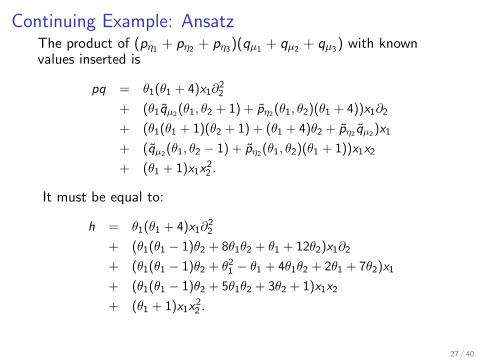
Continuing Example: AnsatzThe product of (pη1 + pη2 + pη3)(qµ1 + qµ2 + qµ3) with knownvalues inserted is
pq = θ1(θ1 + 4)x1∂22
+ (θ1qµ2 (θ1, θ2 + 1) + pη2 (θ1, θ2)(θ1 + 4))x1∂2
+ (θ1(θ1 + 1)(θ2 + 1) + (θ1 + 4)θ2 + pη2 qµ2 )x1
+ (qµ2 (θ1, θ2 − 1) + pη2 (θ1, θ2)(θ1 + 1))x1x2
+ (θ1 + 1)x1x22 .
It must be equal to:
h = θ1(θ1 + 4)x1∂22
+ (θ1(θ1 − 1)θ2 + 8θ1θ2 + θ1 + 12θ2)x1∂2
+ (θ1(θ1 − 1)θ2 + θ21 − θ1 + 4θ1θ2 + 2θ1 + 7θ2)x1
+ (θ1(θ1 − 1)θ2 + 5θ1θ2 + 3θ2 + 1)x1x2
+ (θ1 + 1)x1x22 .
27 / 40

Continuing Example: System of Difference Equations
We first look at equations, linear in p, q:
θ1(θ1 + 4) = θ1(θ1 + 4),(θ1 qµ2
(θ1, θ2 + 1) + pη2· (θ1 + 4)) = (θ1(θ1 − 1)θ2 + 8θ1θ2 + θ1 + 12θ2),
(θ1(θ1 + 1)(θ2 + 1) + (θ1 + 4)θ2 + pη2qµ2
) = (θ1(θ1 − 1)θ2 + θ21 − θ1 + 4θ1θ2 + 2θ1 + 7θ2),
(qµ2(θ1, θ2 − 1) + pη2
· (θ1 + 1)) = (θ1(θ1 − 1)θ2 + 5θ1θ2 + 3θ2 + 1),
(θ1 + 1) = (θ1 + 1).
Putting pη2 on the left hand side we obtain two identities for pη2 ,which result in the equation for qµ2
(θ1(θ1 − 1)θ2 + 8θ1θ2 + θ1 + 12θ2 − θ1qµ2 (θ1, θ2 + 1))(θ1 + 1)
= (θ1(θ1 − 1)θ2 + 5θ1θ2 + 3θ2 + 1− qµ2 (θ1, θ2 − 1))(θ1 + 4).
Ansatz + degree bounds from above: qµ2 is a K-linear expressionin monomials {1, θ1, θ2, θ
21, θ1θ2, θ
22, θ
21θ2, θ1θ
22, θ
21θ
22}.
28 / 40
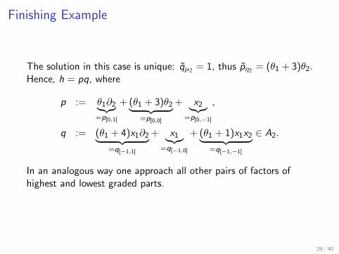
Finishing Example
The solution in this case is unique: qµ2 = 1, thus pη2 = (θ1 + 3)θ2.Hence, h = pq, where
p := θ1∂2︸︷︷︸=p[0,1]
+ (θ1 + 3)θ2︸ ︷︷ ︸=p[0,0]
+ x2︸︷︷︸=p[0,−1]
,
q := (θ1 + 4)x1∂2︸ ︷︷ ︸=q[−1,1]
+ x1︸︷︷︸=q[−1,0]
+ (θ1 + 1)x1x2︸ ︷︷ ︸=q[−1,−1]
∈ A2.
In an analogous way one approach all other pairs of factors ofhighest and lowest graded parts.
29 / 40
Non-CommutativeFactorized Grobner Bases
30 / 40
Factorized Grobner bases – Commutative
I The factorized Grobner approach has been studied extensivelyfor the commutative case (Czapor, 1989b,a; Davenport, 1987;Grabe, 1995a,b).
I Used in Primary Decomposition algorithms.
I Implementations: e.g. in Singular and Reduce.
I Idea: For each factor g of a reducible g during a Grobnercomputation, recursively (tree-like) call the algorithm on thesame generator set, with g being replaced by g .
I Extension: Allows constraints of the type f 6= 0.
Non-commutative case:
I very few possibilities to decompose modules
I no direct analogon of Primary Decomposition
Good news: factorized Grobner approach delivers useful data.
31 / 40
Generalization to Non-Commutative Rings
I Ideals in commutative ring ↔ Varieties
I Ideals in non-commutative ring ↔ Solutions in certain space
I Formal notion of solutions:
Let F be a left A-module for a K-algebra A (space ofsolutions). Let a left A-module M be finitely presented by ann ×m matrix P. Then
SolA(M,F) = {f ∈ Fm : P • f = 0}
is a right EndA(M)-module and a K-vector space.
I Divisors for commutative rings ↔ Right divisors fornon-commutative rings.
I non-commutative novelty: we have to consider all possiblenon-unique maximal right divisors and split Grobnercomputation with respect to them.
32 / 40

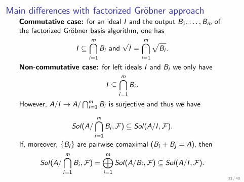
Main differences with factorized Grobner approachCommutative case: for an ideal I and the output B1, . . . ,Bm ofthe factorized Grobner basis algorithm, one has
I ⊆m⋂i=1
Bi and√I =
m⋂i=1
√Bi .
Non-commutative case: for left ideals I and Bi we only have
I ⊆m⋂i=1
Bi .
However, A/I → A/⋂m
i=1 Bi is surjective and thus we have
Sol(A/m⋂i=1
Bi ,F) ⊆ Sol(A/I ,F).
If, moreover, {Bi} are pairwise comaximal (Bi + Bj = A), then
Sol(A/m⋂i=1
Bi ,F) =m⊕i=1
Sol(A/Bi ,F) ⊆ Sol(A/I ,F).
33 / 40

Example
Recall a polynomial from (Tsai, 2000, Example 5.7)
p =(x6 + 2x4 − 3x2)∂2 − (4x5 − 4x4 − 12x2 − 12x)∂
+ (6x4 − 12x3 − 6x2 − 24x − 12) ∈ A1,
with its’ two different factorizations:
p =(x4∂ − x3∂ − 3x3 + 3x2∂ + 6x2 − 3x∂ − 3x + 12)·(x2∂ + x∂ − 3x − 1) ←− q1
=(x4∂ + x3∂ − 4x3 + 3x2∂ − 3x2 + 3x∂ − 6x − 3)·(x2∂ − x∂ − 2x + 4) ←− q2
Our implementation of FGB fgbg.lib in Singular:Pluralreturns (B1,B2) = (〈q1〉, 〈q2〉).
34 / 40

Example
Since 〈p〉 ( B1 ∩ B2
for A := A1 and an arbitrary left A-module F we have
SolA(A/(B1∩B2),F) = SolA(A/B1,F)⊕SolA(A/B2,F)⊆SolA(A/〈p〉,F)
But the space of holomorphic solutions of 〈p〉 at a generic pointx ∈ C is the direct sum of solution spaces of 〈q1〉 and 〈q2〉, that is
SolA(A/〈p〉,Ox) = SolA(A/B1,Ox)⊕ SolA(A/B2,Ox).
35 / 40

Conclusion and Future Work
36 / 40

Future Work
I More criteria for non-commutative FFDs are needed
I Can we detect, whether a given polynomial from a non-FFDhas finite number of factorizations?
I Investigate Finite Factorization Rings (FFRs) instead ofdomains (e.g. integro-differential algebras)
I Algorithms for factoring in finitely presented algebras
I The output of non-commutative factorized Grobner basisalgorithm might contain more structural information
I Implementation of all the algorithms (done for G -algebras):
Latest ncfactor.lib can be found in theSingular:Plural distribution
fgbg.lib (factorized Grobner for G -algebras) will beavailable soon.
37 / 40

Thank you for your attention!
http://www.singular.uni-kl.de
38 / 40

Bibliography I
Abramov, S. A., Le, H., and Li, Z. (2003). OreTools: A Computer Algebra Library for Univariate Ore PolynomialRings. School of Computer Science CS-2003-12, University of Waterloo.
Anderson, D. (1997). Factorization in integral domains, volume 189. CRC Press.
Anderson, D. and Anderson, D. (1992). Elasticity of factorizations in integral domains. Journal of pure and appliedalgebra, 80(3):217–235.
Anderson, D., Anderson, D., and Zafrullah, M. (1990). Factorization in integral domains. Journal of pure andapplied algebra, 69(1):1–19.
Anderson, D. and Mullins, B. (1996). Finite factorization domains. Proceedings of the American MathematicalSociety, 124(2):389–396.
Bell, J. P., Heinle, A., and Levandovskyy, V. (2017). On noncommutative finite factorization domains.Transactions of the American Mathematical Society, 369:2675–2695.
Bueso, J., Gomez-Torrecillas, J., and Verschoren, A. (2003). Algorithmic methods in non-commutative algebra.Applications to quantum groups. Dordrecht: Kluwer Academic Publishers.
Cohn, P. (1963). Noncommutative unique factorization domains. Transactions of the American MathematicalSociety, 109(2):313–331.
Cohn, P. M. (2006). Free ideal rings and localization in general rings, volume 3. Cambridge University Press.
Czapor, S. R. (1989a). Solving algebraic equations: combining Buchberger’s algorithm with multivariatefactorization. Journal of Symbolic Computation, 7(1):49–53.
Czapor, S. R. (1989b). Solving algebraic equations via Buchberger’s algorithm. In Eurocal’87, pages 260–269.Springer.
Davenport, J. H. (1987). Looking at a set of equations. Technical report, School of Mathematical Sciences, TheUniversity of Bath.
Giesbrecht, M. (1998). Factoring in Skew-Polynomial Rings over Finite Fields. Journal of Symbolic Computation,26(4):463–486.
Giesbrecht, M. and Heinle, A. (2012). A Polynomial-Time Algorithm for the Jacobson Form of a Matrix of OrePolynomials. In Computer Algebra in Scientific Computing, pages 117–128. Springer.
39 / 40

Bibliography II
Giesbrecht, M., Heinle, A., and Levandovskyy, V. (2016). Factoring linear differential operators in n variables.Journal of Symbolic Computation, 75:127–148.
Grabe, H.-G. (1995a). On factorized Grobner bases. In Computer algebra in science and engineering, pages 77–89.World Scientific. Citeseer.
Grabe, H.-G. (1995b). Triangular systems and factorized Grobner bases. Springer.
Greuel, G.-M., Levandovskyy, V., Motsak, A., and Schonemann, H. (2016). Plural. A Singular 4-1 Subsystemfor Computations with Non-commutative Polynomial Algebras. Centre for Computer Algebra, TUKaiserslautern. www.singular.uni-kl.de
Heinle, A. and Levandovskyy, V. (2017b) A Factorization Algorithm for G -Algebras and its Applications. Journal ofSymbolic Computation, in press, available online
Heinle, A. and Levandovskyy, V. (2017a) Factorization of Z-homogeneous Polynomials in the First (q-)WeylAlgebra, Springer LNM, to appear. http://arxiv.org/abs/1302.5674
Jacobson, N. (1943). The Theory of Rings. American Mathematical Society.
Kauers, M., Jaroschek, M., and Johansson, F. (2014). Ore Polynomials in Sage. In Gutierrez, J., Schicho, J., andWeimann, M., editors, Computer Algebra and Polynomials, Lecture Notes in Computer Science, pages 105–125.
Melenk, H. and Apel, J. (1994). Reduce package ncpoly: Computation in non-commutative polynomial ideals.Konrad-Zuse-Zentrum Berlin (ZIB), 65.
Tsai, H. (2000). Weyl closure of a linear differential operator. Journal of Symbolic Computation, 29:747–775.
Tsarev, S. (1996). An Algorithm for Complete Enumeration of all Factorizations of a Linear Ordinary DifferentialOperator. In Proceedings of the International Symposium on Symbolic and Algebraic Computation 1996. NewYork, NY: ACM Press.
van Hoeij, M. (1997). Factorization of Differential Operators with Rational Functions Coefficients. 24(5):537–561.
40 / 40


![arXiv:1609.09686v1 [math.CO] 30 Sep 2016 · 2016. 10. 3. · arXiv:1609.09686v1 [math.CO] 30 Sep 2016 STRONG FACTORIZATION PROPERTY OF MACDONALD POLYNOMIALS AND GENERALIZED MACDONALD’S](https://static.fdocuments.net/doc/165x107/60f8fcababd5284a205732f0/arxiv160909686v1-mathco-30-sep-2016-2016-10-3-arxiv160909686v1-mathco.jpg)