Factoring and Discrete Logarithms using PseudorandomWalkssgal018/crypto-book/ch14.pdf · Factoring...

Chapter 14

Factoring and Discrete

Logarithms using

Pseudorandom Walks

This is a chapter from version 1.1 of the book “Mathematics of Public Key Cryptography”by Steven Galbraith, available from http://www.isg.rhul.ac.uk/ sdg/crypto-book/ Thecopyright for this chapter is held by Steven Galbraith.

This book is now completed and an edited version of it will be published by CambridgeUniversity Press in early 2012. Some of the Theorem/Lemma/Exercise numbers may bedifferent in the published version.

Please send an email to [email protected] if you find any mistakes.All feedback on the book is very welcome and will be acknowledged.

This chapter is devoted to the rho and kangaroo methods for factoring and discretelogarithms (which were invented by Pollard) and some related algorithms. These meth-ods use pseudorandom walks and require low storage (typically a polynomial amount ofstorage, rather than exponential as in the time/memory tradeoff). Although the rho fac-toring algorithm was developed earlier than the algorithms for discrete logarithms, thelatter are much more important in practice.1 Hence we focus mainly on the algorithmsfor the discrete logarithm problem.

As in the previous chapter, we assume G is an algebraic group over a finite field Fq

written in multiplicative notation. To solve the DLP in an algebraic group quotient usingthe methods in this chapter one would first lift the DLP to the covering group (thoughsee Section 14.4 for a method to speed up the computation of the DLP in an algebraicgroup by essentially working in a quotient).

14.1 Birthday Paradox

The algorithms in this chapter rely on results in probability theory. The first tool we needis the so-called “birthday paradox”. This name comes from the following application,

1Pollard’s paper [486] contains the remark “We are not aware of any particular need for such indexcalculations” (i.e., computing discrete logarithms) even though [486] cites the paper of Diffie and Hellman.Pollard worked on the topic before hearing of the cryptographic applications. Hence Pollard’s work isan excellent example of research pursued for its intrinsic interest, rather than motivated by practicalapplications.

285

286 CHAPTER 14. PSEUDORANDOM WALKS

which surprises most people: among a set of 23 or more randomly chosen people, theprobability that two of them share a birthday is greater than 0.5 (see Example 14.1.4).

Theorem 14.1.1. Let S be a set of N elements. If elements are sampled uniformly atrandom from S then the expected number of samples to be taken before some element issampled twice is less than

√

πN/2 + 2 ≈ 1.253√N .

The element that is sampled twice is variously known as a repeat, match or collision.For the rest of the chapter, we will ignore the +2 and say that the expected number ofsamples is

√

πN/2.Proof: Let X be the random variable giving the number of elements selected from S(uniformly at random) before some element is selected twice. After l distinct elementshave been selected then the probability that the next element selected is also distinctfrom the previous ones is (1 − l/N). Hence the probability Pr(X > l) is given by

pN,l = 1(1− 1/N)(1− 2/N) · · · (1− (l − 1)/N).

Note that pN,l = 0 when l ≥ N . We now use the standard fact that 1 − x ≤ e−x forx ≥ 0. Hence,

pN,l ≤ 1 e−1/Ne−2/N · · · e−(l−1)/N = e−∑l−1j=0 j/N

= e−12 (l−1)l/N

≤ e−(l−1)2/2N .

By definition, the expected value of X is

∞∑

l=1

lPr(X = l) =

∞∑

l=1

l(Pr(X > l − 1)− Pr(X > l))

=

∞∑

l=0

(l + 1− l) Pr(X > l)

=

∞∑

l=0

Pr(X > l)

≤ 1 +

∞∑

l=1

e−(l−1)2/2N .

We estimate this sum using the integral

1 +

∫ ∞

0

e−x2/2Ndx.

Since e−x2/2N is monotonically decreasing and takes values in [0, 1] the difference between

the value of the sum and the value of the integral is at most 1. Making the change ofvariable u = x/

√2N gives

√2N

∫ ∞

0

e−u2

du.

A standard result in analysis (see Section 11.7 of [339] or Section 4.4 of [635]) is that thisintegral is

√π/2. Hence, the expected value for X is ≤

√

πN/2 + 2. �

The proof only gives an upper bound on the probability of a collision after l trials.A lower bound of e−l

2/2N−l3/6N2

for N ≥ 1000 and 0 ≤ l ≤ 2N log(N) is given in

14.2. THE POLLARD RHO METHOD 287

Wiener [630]; it is also shown that the expected value of the number of trials is>√

πN/2−0.4. A more precise analysis of the birthday paradox is given in Example II.10 of Flajoletand Sedgewick [204] and Exercise 3.1.12 of Knuth [342]. The expected number of samplesis√

πN/2 + 2/3 +O(1/√N).

We remind the reader of the meaning of expected value. Suppose the experiment ofsampling elements of a set S of size N until a collision is found is repeated t times andeach time we count the number l of elements sampled. Then the average of l over alltrials tends to

√

πN/2 as t goes to infinity.

Exercise 14.1.2. Show that the number of elements that need to be selected from S toget a collision with probability 1/2 is

√

2 log(2)N ≈ 1.177√N .

Exercise 14.1.3. One may be interested in the number of samples required when oneis particularly unlucky. Determine the number of trials so that with probability 0.99 onehas a collision. Repeat the exercise for probability 0.999.

The name “birthday paradox” arises from the following application of the result.

Example 14.1.4. In a room containing 23 or more randomly chosen people, the prob-ability is greater than 0.5 that two people have the same birthday. This follows from√

2 log(2)365 ≈ 22.49. Note also that√

π365/2 = 23.944 . . . .

Finally, we mention that the expected number of samples from a set of size N untilk > 1 collisions are found is approximately

√2kN . A detailed proof of this fact is given

by Kuhn and Struik as Theorem 1 of [354].

14.2 The Pollard Rho Method

Let g be a group element of prime order r and let G = 〈g〉. The discrete logarithmproblem (DLP) is: Given h ∈ G to find a, if it exists, such that h = ga. In this sectionwe assume (as is usually the case in applications) that one has already determined thath ∈ 〈g〉.

The starting point of the rho algorithm is the observation that if one can find ai, bi, aj , bj ∈Z/rZ such that

gaihbi = gajhbj (14.1)

and bi 6≡ bj (mod r) then one can solve the DLP as

h = g(ai−aj)(bj−bi)−1 (mod r).

The basic idea is to generate pseudorandom sequences xi = gaihbi of elements inG by iterating a suitable function f : G → G. In other words, one chooses a startingvalue x1 and defines the sequence by xi+1 = f(xi). A sequence x1, x2, . . . is called adeterministic pseudorandom walk. Since G is finite there is eventually a collisionxi = xj for some 1 ≤ i < j as in equation (14.1). This is presented as a collision betweentwo elements in the same walk, but it could also be a collision between two elements indifferent walks. If the elements in the walks look like uniformly and independently chosenelements of G then, by the birthday paradox (Theorem 14.1.1), the expected value of jis√

πr/2.It is important that the function f be designed so that one can efficiently compute

ai, bi ∈ Z/rZ such that xi = gaihbi . The next step xi+1 depends only on the currentstep xi and not on (ai, bi). The algorithms all exploit the fact that when a collision


xi = xj occurs then xi+t = xj+t for all t ∈ N. Pollard’s original proposal used a cycle-finding method due to Floyd to find a self-collision in the sequence; we present this inSection 14.2.2. A better approach is to use distinguished points to find collisions; wepresent this in Section 14.2.4.

14.2.1 The Pseudorandom Walk

Pollard simulates a random function from G to itself as follows. The first step is todecompose G into nS disjoint subsets (usually of roughly equal size) so that G = S0 ∪S1 ∪ · · · ∪ SnS−1. Traditional textbook presentations use nS = 3 but, as explained inSection 14.2.5, it is better to take larger values for nS ; typical values in practice are 32,256 or 2048.

The sets Si are defined using a selection function S : G → {0, . . . , nS − 1} by Si ={g ∈ G : S(g) = i}. For example, in any computer implementation of G one representsan element g ∈ G as a unique2 binary string b(g) and interpreting b(g) as an integer onecould define S(g) = b(g) (mod nS) (taking nS to be a power of 2 makes this computationespecially easy). To obtain different choices for S one could apply an F2-linear map L tothe sequence of bits b(g), so that S(g) = L(b(g)) (mod nS). These simple methods canbe a poor choice in practice, as they are not “sufficiently random”. Some other ways todetermine the partition are suggested in Section 2.3 of Teske [604] and Bai and Brent [24].The strongest choice is to apply a hash function or randomness extractor to b(g), thoughthis may lead to an undesirable computational overhead.

Definition 14.2.1. The rho walks are defined as follows. Precompute gj = gujhvj for0 ≤ j ≤ nS − 1 where 0 ≤ uj, vj < r are chosen uniformly at random. Set x1 = g. Theoriginal rho walk is

xi+1 = f(xi) =

{

x2i if S(xi) = 0xigj if S(xi) = j, j ∈ {1, . . . , nS − 1} (14.2)

The additive rho walk isxi+1 = f(xi) = xigS(xi). (14.3)

An important feature of the walks is that each step requires only one group operation.Once the selection function S and the values uj and vj are chosen, the walk is de-

terministic. Even though these values may be chosen uniformly at random, the functionf itself is not a random function as it has a compact description. Hence, the rho walkscan only be described as pseudorandom. To analyse the algorithm we will consider theexpectation of the running time over different choices for the pseudorandom walk. Manyauthors consider the expectation of the running time over all problem instances and ran-dom choices of the pseudorandom walk; they therefore write “expected running time” forwhat we are calling “average-case expected running time”.

It is necessary to keep track of the decomposition

xi = gaihbi .

The values ai, bi ∈ Z/rZ are obtained by setting a1 = 1, b1 = 0 and updating (for theoriginal rho walk)

ai+1 =

{

2ai (mod r) if S(xi) = 0ai + uS(xi) (mod r) if S(xi) > 0

and bi+1 =

{

2bi (mod r) if S(xi) = 0bi + vS(xi) (mod r) if S(xi) > 0.

(14.4)

2One often uses projective coordinates to speed up elliptic curve arithmetic, so it is natural to useprojective coordinates when implementing these algorithms. But to define the pseudorandom walk oneneeds a unique representation for points, so projective coordinates are not appropriate. See Remark 13.3.2.


Putting everything together, we write

(xi+1, ai+1, bi+1) = walk(xi, ai, bi)

for the random walk function. But it is important to remember that xi+1 only dependson xi and not on (xi, ai, bi).

Exercise 14.2.2. Give the analogue of equation (14.4) for the additive walk.

14.2.2 Pollard Rho Using Floyd Cycle Finding

We present the original version of Pollard rho. A single sequence x1, x2, . . . of groupelements is computed. Eventually there is a collision xi = xj with 0 ≤ i < j. One picturesthe walk as having a tail (which is the part x1, . . . , xi of the walk that is not cyclic)followed by the cycle or head (which is the part xi+1, . . . , xj). Drawn appropriately thisresembles the shape of the greek letter ρ. The tail and cycle (or head) of such a randomwalk have expected length

√

πN/8 (see Flajolet and Odlyzko [203] for proofs of these,and many other, facts).

The goal is to find integers i and j such that xi = xj . It might seem that the onlyapproach is to store all the xi and, for each new value xj , to check if it appears in the list.This approach would use more memory and time than the baby-step-giant-step algorithm.If one were using a truly random walk then one would have to use this approach. Thewhole point of using a deterministic walk which eventually becomes cyclic is to enablebetter methods to find a collision.

Let lt be the length of the tail of the “rho” and lh be the length of the cycle of the“rho”. In other words the first collision is

xlt+lh = xlt . (14.5)

Floyd’s cycle finding algorithm3 is to compare xi and x2i. Lemma 14.2.3 shows thatthis will find a collision in at most lt + lh steps. The crucial advantage of comparing x2iand xi is that it only requires storing two group elements. The rho algorithm with Floydcycle finding is given in Algorithm 16.

Algorithm 16 The rho algorithm

Input: g, h ∈ GOutput: a such that h = ga, or ⊥1: Choose randomly the function walk as explained above2: x1 = g, a1 = 1, b1 = 03: (x2, a2, b2) = walk(x1, a1, b1)4: while (x1 6= x2) do5: (x1, a1, b1) = walk(x1, a1, b1)6: (x2, a2, b2) = walk(walk(x2, a2, b2))7: end while

8: if b1 ≡ b2 (mod r) then9: return ⊥

10: else

11: return (a2 − a1)(b1 − b2)−1 (mod r)

12: end if

3Apparently this algorithm first appears in print in Knuth [342], but is credited there to Floyd.


Lemma 14.2.3. Let the notation be as above. Then x2i = xi if and only if lh | i andi ≥ lt. Further, there is some lt ≤ i < lt + lh such that x2i = xi.

Proof: If xi = xj then we must have lh | (i− j). Hence the first statement of the Lemmais clear. The second statement follows since there is some multiple of lh between lt andlt + lh. �

Exercise 14.2.4. Let p = 347, r = 173, g = 3, h = 11 ∈ F∗p. Let nS = 3. Determine lt

and lh for the values (u1, v1) = (1, 1), (u2, v2) = (13, 17). What is the smallest of i forwhich x2i = xi?

Exercise 14.2.5. Repeat Exercise 14.2.4 for g = 11, h = 3 (u1, v1) = (4, 7) and (u2, v2) =(23, 5).

The smallest index i such that x2i = xi is called the epact. The expected value ofthe epact is conjectured to be approximately 0.823

√

πr/2; see Heuristic 14.2.9.

Example 14.2.6. Let p = 809 and consider g = 89 which has prime order 101 in F∗p.

Let h = 799 which lies in the subgroup generated by g.

Let nS = 4. To define S(g) write g in the range 1 ≤ g < 809, represent thisinteger in its usual binary expansion and then reduce modulo 4. Choose (u1, v1) =(37, 34), (u2, v2) = (71, 69), (u3, v3) = (76, 18) so that g1 = 343, g2 = 676, g3 = 627. Onecomputes the table of values (xi, ai, bi) as follows:

i xi ai bi S(xi)1 89 1 0 12 594 38 34 23 280 8 2 04 736 16 4 05 475 32 8 36 113 7 26 17 736 44 60 0

It follows that lt = 4 and lh = 3 and so the first collision detected by Floyd’s methodis x6 = x12. We leave as an exercise to verify that the discrete logarithm in this case is50.

Exercise 14.2.7. Let p = 569 and let g = 262 and h = 5 which can be checked to haveorder 71 modulo p. Use the rho algorithm to compute the discrete logarithm of h to thebase g modulo p.

Exercise 14.2.8. One can simplify Definition 14.2.1 and equation (14.4) by replacing gjby either guj or hvj (independently for each j). Show that this saves one modular additionin each iteration of the algorithm. Explain why this optimisation should not affect thesuccess of the algorithm, as long as the walk uses all values for S(xi) with roughly equalprobability.

Algorithm 16 always terminates, but there are several things that can go wrong:

• The value (b1 − b2) may not be invertible modulo r.

Hence, we can only expect to prove that the algorithm succeeds with a certainprobability (extremely close to 1).


• The cycle may be very long (as big as r) in which case the algorithm is slower thanbrute force search.

Hence, we can only expect to prove an expected running time for the algorithm. Werecall that the expected running time in this case is the average, over all choices forthe function walk, of the worst-case running time of the algorithm over all probleminstances.

Note that the algorithm always halts, but it may fail to output a solution to the DLP.Hence, this is a Monte Carlo algorithm.

It is an open problem to give a rigorous running time analysis for the rho algorithm.Instead it is traditional to make the heuristic assumption that the pseudorandom walkdefined above behaves sufficiently close to a random walk. The rest of this section isdevoted to showing that the heuristic running time of the rho algorithm with Floyd cyclefinding is (3.093 + o(1))

√r group operations (asymptotic as r → ∞).

Before stating a precise heuristic we determine an approximation to the expected valueof the epact in the case of a truly random walk.4

Heuristic 14.2.9. Let xi be a sequence of elements of a group G of order r obtained asabove by iterating a random function f : G → G. Then the expected value of the epact(i.e., the smallest positive integer i such that x2i = xi) is approximately (ζ(2)/2)

√

πr/2 ≈0.823

√

πr/2, where ζ(2) = π2/6 is the value of the Riemann zeta function at 2.

Argument: Fix a specific sequence xi and let l be the length of the rho, so that xl+1

lies in {x1, x2, . . . , xl}. Since xl+1 can be any one of the xi, the cycle length lh can beany value 1 ≤ lh ≤ l and each possibility happens with probability 1/l.

The epact is the smallest multiple of lh which is bigger than lt = l − lh. Hence, ifl/2 ≤ lh ≤ l then the epact is lh, if l/3 ≤ lh < l/2 then the epact is 2lh. In general, ifl/(k+1) ≤ lh < l/k then the epact is klh. The largest possible value of the epact is l− 1,which occurs when lh = 1.

The expected value of the epact when the rho has length l is therefore

El =

∞∑

k=1

l∑

lh=1

klhPl(k, lh)

where Pl(k, lh) is the probability that klh is the epact. By the above discussion, P (k, lh) =1/l if l/(k + 1) ≤ lh < l/k or (k, lh) = (1, l) and zero otherwise. Hence

El =1l

l−1∑

k=1

k∑

l/(k+1)≤lh<l/kor (k,lh)=(1,l)

lh

Approximating the inner sum as 12

(

(l/k)2 − (l/(k + 1))2)

gives

El ≈ l2

∞∑

k=1

k(

1k2 − 1

(k+1)2

)

.

Now, k(1/k2 − 1/(k + 1)2) = 1/k − 1/(k + 1) + 1/(k + 1)2 and

∞∑

k=1

(1/k − 1/(k + 1)) = 1 and

∞∑

k=1

1/(k + 1)2 = ζ(2)− 1.

4I thank John Pollard for showing me this argument.


Hence El ≈ l/2(1+ ζ(2)− 1). It is well-known that ζ(2) ≈ 1.645. Finally, write Pr(e) forthe probability the epact is e, Pr(l) for the probability the rho length is l, and Pr(e | l)for the conditional probability that the epact is e given that the rho has length l. Theexpectation of e is then

E(e) =

∞∑

e=1

ePr(e) =

∞∑

e=1

e

∞∑

l=1

Pr(e | l) Pr(l)

=∞∑

l=1

Pr(l)

( ∞∑

e=1

ePr(e | l))

=

∞∑

l=1

Pr(l)El ≈ (ζ(2)/2)E(l)

which completes the argument. �

We can now give a heuristic analysis of the running time of the algorithm. We makethe following assumption, which we believe is reasonable when r is sufficiently large,nS > log(r) and when the function walk is chosen at random (from the set of all walkfunctions specified in Section 14.2.1).

Heuristic 14.2.10.

1. The expected value of the epact is (0.823 + o(1))√

πr/2.

2. The value∑lt+lh−1

i=ltvS(xi) (mod r) is uniformly distributed in Z/rZ.

Theorem. Let the notation be as above and assume Heuristic 14.2.10. Then the rhoalgorithm with Floyd cycle finding has expected running time of (3.093 + o(1))

√r group

operations. The probability the algorithm fails is negligible.

Proof: The number of iterations of the main loop in Algorithm 16 is the epact. ByHeuristic 14.2.10 the expected value of the epact is (0.823 + o(1))

√

πr/2.Algorithm 16 performs three calls to the function walk in each iteration. Each call to

walk results in one group operation and two additions modulo r (we ignore these additionsas they cost significantly less than a group operation). Hence the expected number ofgroup operations is 3(0.823 + o(1))

√

πr/2 ≈ (3.093 + o(1))√r as claimed.

The algorithm fails only if b2i ≡ bi (mod r). We have galthblt = galt+lhhblt+lh fromwhich it follows that alt+lh = alt + u, blt+lh = blt + v where guhv = 1. Precisely,

v ≡ blt+lh − blt ≡∑lt+lh−1

i=ltvS(xi) (mod r).

Write i = lt+ i′ for some 0 ≤ i′ < lh and bi = blt +w. Assume lh ≥ 2 (the probabilitythat lh = 1 is negligible). Then 2i = lt+xlh+ i

′ for some integer 1 ≤ x < (lt+2lh)/lh < rand so b2i = blt + xv + w. It follows that b2i ≡ bi (mod r) if and only if r | v.

According to Heuristic 14.2.10 the value v is uniformly distributed in Z/rZ and so theprobability it is zero is 1/r, which is a negligible quantity in the input size of the problem.�

14.2.3 Other Cycle Finding Methods

Floyd cycle finding is not a very efficient way to find cycles. Though any cycle findingmethod requires computing at least lt + lh group operations, Floyd’s method needs onaverage 2.47(lt + lh) group operations (2.47 is three times the expected value of theepact). Also, the “slower” sequence xi is visiting group elements which have alreadybeen computed during the walk of the “faster” sequence x2i. Brent [98] has given an


improved cycle finding method5 that still only requires storage for two group elementsbut which requires fewer group operations. Montgomery has given an improvement toBrent’s method in [435].

One can do even better by using more storage, as was shown by Sedgewick, Szymanskiand Yao [534], Schnorr and Lenstra [526] (also see Teske [602]) and Nivasch [466]. The rhoalgorithm using Nivasch cycle finding has the optimal expected running time of

√

πr/2 ≈1.253

√r group operations and is expected to require polynomial storage.

Finally, a very efficient way to find cycles is to use distinguished points. More impor-tantly, distinguished points allow us to think about the rho method in a different wayand this leads to a version of the algorithm that can be parallelised. We discuss this inthe next section. Hence, in practice one always uses distinguished points.

14.2.4 Distinguished Points and Pollard Rho

The idea of using distinguished points in search problems apparently goes back to Rivest.The first application of this idea to computing discrete logarithms is by van Oorschot andWiener [472].

Definition 14.2.11. An element g ∈ G is a distinguished point if its binary rep-resentation b(g) satisfies some easily checked property. Denote by D ⊂ G the set ofdistinguished points. The probability #D/#G that a uniformly chosen group element isa distinguished point is denoted θ.

A typical example is the following.

Example 14.2.12. Let E be an elliptic curve over Fp. A point P ∈ E(Fp) that is notthe point at infinity is represented by an x-coordinate 0 ≤ xP < p and a y-coordinate0 ≤ yP < p. Let H be a hash function, whose output is interpreted as being in Z≥0.

Fix an integer nD. Define D to be the points P ∈ E(Fp) such that the nD leastsignificant bits of H(xP ) are zero. Note that OE 6∈ D. In other words

D = {P = (xP , yP ) ∈ E(Fp) : H(xP ) ≡ 0 (mod 2nD ) where 0 ≤ xP < p}.

Then θ ≈ 1/2nD .

The rho algorithm with distinguished points is as follows. First, choose integers 0 ≤a1, b1 < r uniformly and independently at random, compute the group element x1 =ga1hb1 and run the usual deterministic pseudorandom walk until a distinguished pointxn = ganhbn is found. Store (xn, an, bn) in some easily searched data structure (searchableon xn). Then choose a fresh randomly chosen group element x1 = ga1hb1 and repeat.Eventually two walks will visit the same group element, in which case their paths willcontinue to the same distinguished point. Once a distinguished group element is foundtwice then the DLP can be solved with high probability.

Exercise 14.2.13. Write down pseudocode for this algorithm.

We stress the most significant difference between this method and the method of theprevious section: the previous method had one long walk with a tail and a cycle, whereasthe new method has many short walks. Note that this algorithm does not require self-collisions in the walk and so there is no ρ shape anymore; the word “rho” in the name ofthe algorithm is therefore a historical artifact, not an intuition about how the algorithmworks.

5This was originally developed to speed up the Pollard rho factoring algorithm.


Note that, since the group is finite, collisions must eventually occur, and so the algo-rithm halts. But the algorithm may fail to solve the DLP (with low probability). Hence,this is a Monte Carlo algorithm.

In the analysis we assume that we are sampling group elements (we sometimes callthem “points”) uniformly and independently at random. It is important to determine theexpected number of steps before landing on a distinguished point.

Lemma 14.2.14. Let θ be the probability that a randomly chosen group element is adistinguished point. Then

1. The probability that one chooses α/θ group elements, none of which are distin-guished, is approximately e−α when 1/θ is large.

2. The expected number of group elements to choose before getting a distinguished pointis 1/θ.

3. If one has already chosen i group elements, none of which are distinguished, then theexpected number of group elements to further choose before getting a distinguishedpoint is 1/θ.

Proof: The probability that i chosen group elements are not distinguished is (1− θ)i. Sothe probability of choosing α/θ points, none of which are distinguished, is

(1− θ)α/θ ≤(

e−θ)α/θ

= e−α.

The second statement is the standard formula for the expected value of a geometricrandom variable, see Example A.14.1.

For the final statement6, suppose one has already sampled i points without finding adistinguished point. Since the trials are independent, the probability of choosing a furtherj points which are not distinguished remains (1−θ)j. Hence the expected number of extrapoints to be chosen is still 1/θ. �

We now make the following assumption. We believe this is reasonable when r issufficiently large, nS > log(r), distinguished points are sufficiently common and specifiedusing a good hash function (and hence, D is well distributed), θ > log(r)/

√r and when

the function walk is chosen at random.

Heuristic 14.2.15.

1. Walks reach a distinguished point in significantly fewer than√r steps (in other

words, there are no cycles in the walks and walks are not excessively longer than1/θ).7

2. The expected number of group elements sampled before a collision is√

πr/2.

Theorem 14.2.16. Let the notation be as above and assume Heuristic 14.2.15. Then therho algorithm with distinguished points has expected running time of (

√

π/2+ o(1))√r ≈

(1.253 + o(1))√r group operations. The probability the algorithm fails is negligible.

Proof: Heuristic 14.2.15 states there are no cycles or “wasted” walks (in the sense thattheir steps do not contribute to potential collisions). Hence, before the first collision,after N steps of the algorithm we have visited N group elements. By Heuristic 14.2.15,

6This is the “apparent paradox” mentioned in footnote 7 of [472].7More realistically, one could assume that only a negligibly small proportion of the walks fall into a

cycle before hitting a distinguished point.


the expected number of group elements to be sampled before the first collision is√

πr/2.The collision is not detected until walks hit a distinguished point, which adds a further2/θ to the number of steps. Hence, the total number of steps (calls to the function walk)in the algorithm is

√

πr/2 + 2/θ. Since 2/θ < 2√r/ log(r) = o(1)

√r, the result follows.

Let x = gaihbi = gajhbj be the collision. Since the starting values ga0hb0 are chosenuniformly and independently at random, the values bi and bj are uniformly and indepen-dently random. It follows that bi ≡ bj (mod r) with probability 1/r, which is a negligiblequantity in the input size of the problem. �

Exercise 14.2.17. Show that if θ = log(r)/√r then the expected storage of the rho

algorithm, assuming it takes O(√r) steps, is O(log(r)) group elements (which is typically

O(log(r)2) bits).

Exercise 14.2.18. The algorithm requires storing a triple (xn, an, bn) for each distin-guished point. Give some strategies to reduce the number of bits that need to be stored.

Exercise 14.2.19. Let G = 〈g1, g2〉 be a group of order r2 and exponent r. Design arho algorithm that, on input h ∈ G outputs (a1, a2) such that h = ga11 ga22 . Determine thecomplexity of this algorithm.

Exercise 14.2.20. Show that the Pollard rho algorithm with distinguished points hasbetter average-case running time than the baby-step-giant-step algorithm (see Exer-cises 13.3.3 and 13.3.4).

Exercise 14.2.21. Explain why taking D = G (i.e., all group elements distinguished)leads to an algorithm that is much slower than the baby-step-giant-step algorithm.

Suppose one is given g, h1, . . . , hL (where 1 < L < r1/4) and is asked to find all ai for1 ≤ i ≤ L such that hi = gai . Kuhn and Struik [354] propose and analyse a method tosolve all L instances of the DLP, using Pollard rho with distinguished points, in roughly√2rL group operations. A crucial trick, attributed to Silverman and Stapleton, is that

once the i-th DLP is known one can re-write all distinguished points gahbi in the form

ga′

. As noted by Hitchcock, Montague, Carter and Dawson [286] one must be careful tochoose a random walk function that does not depend on the elements hi (however, therandom starting points do depend on the hi).

Exercise 14.2.22. Write down pseudocode for the Kuhn-Struik algorithm for solving Linstances of the DLP, and explain why the algorithm works.

Section 14.2.5 explains why the rho algorithm with distinguished points can be easilyparallelised. That section also discusses a number of practical issues relating to the useof distinguished points.

Cheon, Hong and Kim [132] sped up Pollard rho in F∗p by using a “look ahead”

strategy; essentially they determine in which partition the next value of the walk lies,without performing a full group operation. A similar idea for elliptic curves has beenused by Bos, Kaihara and Kleinjung [89].

14.2.5 Towards a Rigorous Analysis of Pollard Rho

Theorem 14.2.16 is not satisfying since Heuristic 14.2.15 is essentially equivalent to thestatement “the rho algorithm has expected running time (1 + o(1))

√

πr/2 group opera-tions”. The reason for stating the heuristic is to clarify exactly what properties of the


pseudorandom walk are required. The reason for believing Heuristic 14.2.15 is that exper-iments with the rho algorithm (see Section 14.4.3) confirm the estimate for the runningtime.

Since the algorithm is fundamental to an understanding of elliptic curve cryptography(and torus/trace methods) it is natural to demand a complete and rigorous treatmentof it. Such an analysis is not yet known, but in this section we mention some partialresults on the problem. The methods used to obtain the results are beyond the scope ofthis book, so we do not give full details. Note that all existing results are in an idealisedmodel where the selection function S is a random function.

We stress that, in practice, the algorithm behaves as the heuristics predict. Further-more, from a cryptographic point of view, it is sufficient for the task of determining keysizes to have a lower bound on the running time of the algorithm. Hence, in practice, theabsence of proved running time is not necessarily a serious issue.

The main results for the original rho walk (with nS = 3) are due to Horwitz andVenkatesan [293], Miller and Venkatesan [425], and Kim, Montenegro, Peres and Tetali [336,335]. The basic idea is to define the rho graph, which is a directed graph with vertexset 〈g〉 and an edge from x1 to x2 if x2 is the next step of the walk when at x1. Fix aninteger n. Define the distribution Dn on 〈g〉 obtained by choosing uniformly at randomx1 ∈ 〈g〉, running the walk for n steps, and recording the final point in the walk. Thecrucial property to study is the mixing time which, informally, is the smallest integern such that Dn is “sufficiently close” to the uniform distribution. For these results, thesquaring operation in the original walk is crucial. We state the main result of Miller andVenkatesan [425] below.

Theorem 14.2.23. (Theorem 1.1 of [425]) Fix ǫ > 0. Then the rho algorithm using theoriginal rho walk with nS = 3 finds a collision in Oǫ(

√r log(r)3) group operations with

probability at least 1− ǫ, where the probability is taken over all partitions of 〈g〉 into threesets S1, S2 and S3. The notation Oǫ means that the implicit constant in the O dependson ǫ.

Kim, Montenegro, Peres and Tetali improved this result in [335] to the desired Oǫ(√r)

group operations. Note that all these works leave the implied constant in the O unspeci-fied.

Note that the idealised model of S being a random function is not implementablewith constant (or even polynomial) storage. Hence, these results cannot be applied to thealgorithm presented above, since our selection functions S are very far from uniformlychosen over all possible partitions of the set 〈g〉. The number of possible partitions of 〈g〉into three subsets of equal size is (for convenience suppose that 3 | r)

(

r

r/3

)(

2r/3

r/3

)

which, using(

ab

)

≥ (a/b)b, is at least 6r/3. On the other hand, a selection functionparameterised by a “key” of c log2(r) bits (e.g., a selection function obtained from akeyed hash function) only leads to rc different partitions.

Sattler and Schnorr [512] and Teske [603] have considered the additive rho walk. Onekey feature of their work is to discuss the effect of the number of partitions nS. Sattlerand Schnorr show (subject to a conjecture) that if nS ≥ 8 then the expected runningtime for the rho algorithm is c

√

πr/2 group operations for an explicit constant c. Teskeshows, using results of Hildebrand, that the additive walk should approximate the uniformdistribution after fewer than

√r steps once nS ≥ 6. She recommends using the additive

14.3. DISTRIBUTED POLLARD RHO 297

walk with nS ≥ 20 and, when this is done, conjectures that the expected cycle length is≤ 1.3

√r (compared with the theoretical ≈ 1.2533

√r).

Further motivation for using large nS is given by Brent and Pollard [99], Arney andBender [13] and Blackburn and Murphy [59]. They present heuristic arguments that theexpected cycle length when using nS partitions is

√

cnSπr/2 where cnS = nS/(nS − 1).This heuristic is supported by the experimental results of Teske [603]. Let G = 〈g〉. Theiranalysis considers the directed graph formed from iterating the function walk : G → G(i.e., the graph with vertex set G and an edge from g to walk(g)). Then, for a randomlychosen graph of this type, nS/(nS − 1) is the variance of the in-degree for this graph,which is the same as the expected value of n(x) = #{y ∈ G : y 6= x, walk(y) = walk(x)}.

Finally, when using equivalence classes (see Section 14.4) there are further advantagesin taking nS to be large.

14.3 Distributed Pollard Rho

In this section we explain how the Pollard rho algorithm can be parallelised. Rather thana parallel computing model we consider a distributed computing model. In this modelthere is a server and NP ≥ 1 clients (we also refer to the clients as processors). Thereis no shared storage or direct communication between the clients. Instead, the server cansend messages to clients and each client can send messages to the server. In general weprefer to minimise the amount of communication between server and clients.8

To solve an instance of the discrete logarithm problem the server will activate a numberof clients, providing each with its own individual initial data. The clients will run the rhopseudorandom walk and occasionally send data back to the server. Eventually the serverwill have collected enough information to solve the problem, in which case it sends allclients a termination instruction. The rho algorithm with distinguished points can verynaturally be used in this setting.

The best one can expect for any distributed computation is a linear speedup comparedwith the serial case (since if the overall total work in the distributed case was less thanthe serial case then this would lead to a faster algorithm in the serial case). In otherwords, with NP clients we hope to achieve a running time proportional to

√r/NP .

14.3.1 The Algorithm and its Heuristic Analysis

All processors perform the same pseudorandom walk (xi+1, ai+1, bi+1) = walk(xi, ai, bi)as in Section 14.2.1, but each processor starts from a different random starting point.Whenever a processor hits a distinguished point then it sends the triple (xi, ai, bi) to theserver and re-starts its walk at a new random point (x0, a0, b0). If one processor ever visitsa point visited by another processor then the walks from that point agree and both walksend at the same distinguished point. When the server receives two triples (x, a, b) and(x, a′, b′) for the same group element x but with b 6≡ b′ (mod r) then it has gahb = ga

′

hb′

and can solve the DLP as in the serial (i.e., non-parallel) case. The server thereforecomputes the discrete logarithm problem and sends a terminate signal to all processors.Pseudocode for both server and clients are given by Algorithms 17 and 18. By design, ifthe algorithm halts then the answer is correct.

We now analyse the performance of this algorithm. To get a clean result we assumethat no client ever crashes, that communications between server and client are perfectly

8There are numerous examples of such distributed computation over the internet. Two notable ex-amples are the Great Internet Mersenne Primes Search (GIMPS) and the Search for ExtraterrestrialIntelligence (SETI). One observes that the former search has been more successful than the latter.


Algorithm 17 The distributed rho algorithm: Server side

Input: g, h ∈ GOutput: c such that h = gc

1: Randomly choose a walk function walk(x, a, b)2: Initialise an easily searched structure L (sorted list, binary tree etc) to be empty3: Start all processors with the function walk4: while DLP not solved do

5: Receive triples (x, a, b) from clients and insert into L6: if first coordinate of new triple (x, a, b) matches existing triple (x, a′, b′) then7: if b′ 6≡ b (mod r) then8: Send terminate signal to all clients9: return (a− a′)(b′ − b)−1 (mod r)

10: end if

11: end if

12: end while

Algorithm 18 The distributed rho algorithm: Client side

Input: g, h ∈ G, function walk1: while terminate signal not received do

2: Choose uniformly at random 0 ≤ a, b < r3: Set x = gahb

4: while x 6∈ D do

5: (x, a, b) = walk(x, a, b)6: end while

7: Send (x, a, b) to server8: end while

14.3. DISTRIBUTED POLLARD RHO 299

reliable, that all clients have the same computational efficiency and are running continu-ously (in other words, each processor computes the same number of group operations inany given time period).

It is appropriate to ignore the computation performed by the server and instead tofocus on the number of group operations performed by each client running Algorithm 18.Each execution of the function walk(x, a, b) involves a single group operation. We mustalso count the number of group operations performed in line 3 of Algorithm 18; thoughthis term is negligible if walks are long on average (i.e., if D is a sufficiently small subsetof G).

It is an open problem to give a rigorous analysis of the distributed rho method. Hence,we make the following heuristic assumption. We believe this assumption is reasonablewhen r is sufficiently large, nS is sufficiently large, log(r)/

√r < θ, the set D of dis-

tinguished points is determined by a good hash function, the number NP of clients issufficiently small (e.g., NP < θ

√

πr/2/ log(r), see Exercise 14.3.3), the function walk ischosen at random.

Heuristic 14.3.1.

1. The expected number of group elements to be sampled before the same element issampled twice is

√

πr/2.

2. Walks reach a distinguished point in significantly fewer than√r/NP steps (in other

words, there are no cycles in the walks and walks are not excessively long). Morerealistically, one could assume that only a negligible proportion of the walks fallinto a cycle before hitting a distinguished point.

Theorem 14.3.2. Let the notation be as above, in particular, let NP be the (fixed, in-dependent of r) number of clients. Let θ the probability that a group element is a dis-tinguished point and suppose log(r)/

√r < θ. Assume Heuristic 14.3.1 and the above

assumptions about the the reliability and equal power of the processors hold. Then the ex-pected number of group operations performed by each client of the distributed rho methodis (1 + 2 log(r)θ)

√

πr/2/NP +1/θ group operations. This is (√

π/2/NP + o(1))√r group

operations when θ < 1/ log(r)2. The storage requirement on the server is θ√

πr/2 +NPpoints.

Proof: Heuristic 14.3.1 states that we expect to sample√

πr/2 group elements in totalbefore a collision arises. Since this work is distributed over NP clients of equal speedit follows that each client is expected to call the function walk about

√

πr/2/NP times.

The total number of group operations is therefore√

πr/2/NP plus 2 log(r)θ√

πr/2/NPfor the work of line 3 of Algorithm 18. The server will not detect the collision until thesecond client hits a distinguished point, which is expected to take 1/θ further steps bythe heuristic (part 3 of Lemma 14.2.14). Hence each client needs to run an expected√

πr/2/NP + 1/θ steps of the walk.

Of course, a collision gahb = ga′

hb′

can be useless in the sense that b′ ≡ b (mod r).A collision implies a′ + cb′ ≡ a + cb (mod r) where h = gc; there are r such pairs(a′, b′) for each pair (a, b). Since each walk starts with uniformly random values (a0, b0)it follows that the values (a, b) are uniformly distributed over the r possibilities. Hencethe probability of a collision being useless is 1/r and the expected number of collisionsrequired is 1.

Each processor runs for√

πr/2/NP + 1/θ steps and therefore is expected to send

θ√

πr/2/NP + 1 distinguished points in its lifetime. The total number of points to store

is therefore θ√

πr/2 +NP . �


Exercise 14.2.17 shows that the complexity in the case NP = 1 can be taken to be(1 + o(1))

√

πr/2 group operations with polynomial storage.

Exercise 14.3.3. When distributing the algorithm it is important to ensure that, withvery high probability, each processor finds at least one distinguished point in less than itstotal expected running time. Show that this will be the case if 1/θ ≤

√

πr/2/ (NP log(r)).

Schulte-Geers [532] analyses the choice of θ and shows that Heuristics 14.2.15 and 14.3.1are not valid asymptotically if θ = o(1/

√r) as r → ∞ (for example, walks in this situation

are more likely to fall into a cycle than to hit a distinguished point). In any case, sinceeach processor only travels a distance of

√

πr/2/NP it follows we should take θ > NP /√r.

In practice one tends to determine the available storage first (say, c group elements wherec > 109) and to set θ = c/

√

πr/2 so that the total number of distinguished points vis-ited is expected to be c. The results of [532] validate this approach. In particular, itis extremely unlikely that there is a self-collision (and hence a cycle) before hitting adistinguished point.

14.4 Speeding up the Rho Algorithm using Equiva-

lence Classes

Gallant, Lambert and Vanstone [231] and Wiener and Zuccherato [631] showed that onecan speed up the rho method in certain cases by defining the pseudorandom walk not onthe group 〈g〉 but on a set of equivalence classes. This is essentially the same thing asworking in an algebraic group quotient instead of the algebraic group.

Suppose there is an equivalence relation on 〈g〉. Denote by x the equivalence classof x ∈ 〈g〉. Let NC be the size of a generic equivalence class. We require the followingproperties:

1. One can define a unique representative x of each equivalence class x.

2. Given (xi, ai, bi) such that xi = gaihbi then one can efficiently compute (xi, ai, bi)

such that xi = gaihbi .

We give some examples in Section 14.4.1 below.One can implement the rho algorithm on equivalence classes by defining a pseudoran-

dom walk function walk(xi, ai, bi) as in Definition 14.2.1. More precisely, set x1 = g, a1 =1, b1 = 0 and define the sequence xi by (this is the “original walk”)

xi+1 = f(xi) =

{

x2i if S(xi) = 0xigj if S(xi) = j, j ∈ {1, . . . , nS − 1} (14.6)

where the selection function S and the values gj = gujhvj are as in Definition 14.2.1.When using distinguished points one defines an equivalence class to be distinguished ifthe unique equivalence class representative has the distinguished property.

There is a very serious problem with cycles that we do not discuss yet; See Sec-tion 14.4.2 for the details.

Exercise 14.4.1. Write down the formulae for updating the values ai and bi in thefunction walk.

Exercise 14.4.2. Write pseudocode for the distributed rho method on equivalence classes.

14.4. USING EQUIVALENCE CLASSES 301

Theorem 14.4.3. Let G be a group and g ∈ G of order r. Suppose there is an equivalencerelation on 〈g〉 as above. Let NC be the generic size of an equivalence class. Let C1 bethe number of bit operations to perform a group operation in 〈g〉 and C2 the number ofbit operations to compute a unique equivalence class representative xi (and to compute

ai, bi).

Consider the rho algorithm as above (ignoring the possibility of useless cycles, seeSection 14.4.2 below). Under a heuristic assumption for equivalence classes analogous toHeuristic 14.2.15 the expected time to solve the discrete logarithm problem is

(√

π

2NC+ o(1)

)√r (C1 + C2)

bit operations. As usual, this becomes (√

π/2NC + o(1))√r/NP (C1 + C2) bit operations

per client when using NP processors of equal computational power.

Exercise 14.4.4. Prove this theorem.

Theorem 14.4.3 assumes a perfect random walk. For walks defined on nS partitions ofthe set of equivalence classes it is shown in Appendix B of [25] (also see Section 2.2 of [91])that one predicts a slightly improved constant than the usual factor cnS = nS/(nS − 1)mentioned at the end of Section 14.2.5.

We mention a potential “paradox” with this idea. In general, computing a uniqueequivalence class representative involves listing all elements of the equivalence class, andhence needs O(NC) bit operations. Hence, naively, the running time is O(

√

NCπr/2)bit operations, which is worse than doing the rho algorithm without equivalence classes.However, in practice one only uses this method when C2 < C1, in which case the speedupcan be significant.

14.4.1 Examples of Equivalence Classes

We now give some examples of useful equivalence relations on some algebraic groups.

Example 14.4.5. For a group G with efficiently computable inverse (e.g., elliptic curvesE(Fq) or algebraic tori Tn with n > 1 (e.g., see Section 6.3)) one can define the equivalencerelation x ≡ x−1. We have NC = 2 (though note that some elements, namely theidentity and elements of order 2, are equal to their inverse so these classes have size 1).If xi = gaihbi then clearly x−1 = g−aih−bi . One defines a unique representative x forthe equivalence class by, for example, imposing a lexicographical ordering on the binaryrepresentation of the elements in the class.

We can generalise this example as follows.

Example 14.4.6. Let G be an algebraic group over Fq with an automorphism groupAut(G) of size NC (see examples in Sections 9.4 and 11.3.3). Suppose that for g ∈ Gof order r one has ψ(g) ∈ 〈g〉 for each ψ ∈ Aut(G). Furthermore, assume that for eachψ ∈ Aut(G) one can efficiently compute the eigenvalue λψ ∈ Z such that ψ(g) = gλψ .Then for x ∈ G one can define x = {ψ(x) : ψ ∈ Aut(G)}.

Again, one defines x by listing the elements of x as bitstrings and choosing the firstone under lexicographical ordering.

Another important class of examples comes from orbits under the Frobenius map.


Example 14.4.7. Let G be an algebraic group defined over Fq but with group consideredover Fqd (for examples see Sections 11.3.2 and 11.3.3). Let πq be the q-power Frobeniusmap on G(Fqd). Let g ∈ G(Fqd) and suppose that πq(g) = gλ ∈ 〈g〉 for some knownλ ∈ Z.

Define the equivalence relation on G(Fqd) so that the equivalence class of x ∈ G(Fqd)is the set x = {πiq(x) : 0 ≤ i < d}. We assume that, for elements x of interest, x ⊆ 〈g〉.Then NC = d, though there can be elements defined over proper subfields for which theequivalence class is smaller.

If one uses a normal basis for Fqd over Fq then one can efficiently compute the elementsπiq(x) and select a unique representative of each equivalence class using a lexicographicalordering of binary strings.

Example 14.4.8. For some groups (e.g., Koblitz elliptic curves E/F2 considered as agroup over F2m ; see Exercise 9.10.11) we can combine both equivalence classes above. Letm be prime, #E(F2m) = hr for some small cofactor h, and P ∈ E(F2m) of order r. Thenπ2(P ) ∈ 〈P 〉 and we define the equivalence class P = {±πi2(P ) : 0 ≤ i < m} of size 2m.Since m is odd, this class can be considered as the orbit of P under the map −π2. Thedistributed rho algorithm on equivalence classes for such curves is expected to requireapproximately

√

π2m/(4m) group operations.

14.4.2 Dealing with Cycles

One problem that can arise is walks that fall into a cycle before they reach a distinguishedpoint. We call these useless cycles.

Exercise 14.4.9. Suppose the equivalence relation is such that x ≡ x−1. Fix xi = xiand let xi+1 = xig. Suppose xi+1 = x−1

i+1 and that S(xi+1) = S(xi). Show that xi+2 ≡ xiand so there is a cycle of order 2. Suppose the equivalence classes generically have sizeNC . Show, under the assumptions that the function S is perfectly random and that x isa randomly chosen element of the equivalence class, that the probability that a randomlychosen xi leads to a cycle of order 2 is 1/(NCnS).

A theoretical discussion of cycles was given in [231] and by Duursma, Gaudry andMorain [185]. An obvious way to reduce the probability of cycles is to take nS to bevery large compared with the average length 1/θ of walks. However, as argued by Bos,Kleinjung and Lenstra [91], large values for nS can lead to slower algorithms (for example,due to the fact that the precomputed steps do not all fit in cache memory). Hence, asExercise 14.4.9 shows, useless cycles will be regularly encountered in the algorithm. Thereare several possible ways to deal with this issue. One approach is to use a “look-ahead”technique to avoid falling in 2-cycles. Another approach is to detect small cycles (e.g.,by storing a fixed number of previous values of the walk or, at regular intervals, usinga cycle-finding algorithm for a small number of steps) and to design a well-defined exitstrategy for short cycles; Gallant, Lambert and Vanstone call this collapsing the cycle;see Section 6 of [231]. To collapse a cycle one must be able to determine a well-definedelement in it; from there one can take a step (different to the steps used in the cycle fromthat point) or use squaring to exit the cycle. All these methods require small amountsof extra computation and storage, though Bernstein, Lange and Schwabe [56] argue thatthe additional overhead can be made negligible. We refer to [56, 91] for further discussionof these issues.

Gallant, Lambert and Vanstone [231] presented a different walk that does not, ingeneral, lead to short cycles. Let G be an algebraic group with an efficiently computableendomorphism ψ of order m (i.e., ψm = ψ ◦ · · · ◦ ψ is the identity map). Let g ∈ G of

14.4. USING EQUIVALENCE CLASSES 303

order r be such that ψ(g) = gλ so that ψ(x) = xλ for all x ∈ 〈g〉. Define the equivalenceclasses x = {ψj(x) : 0 ≤ j < m}. We define a pseudorandom sequence xi = gaihbi byusing x to select an endomorphism (1 + ψj) and then acting on xi with this map. Moreprecisely, j is some function of x (e.g., the function S in Section 14.2.1) and

xi+1 = (1 + ψj)xi = xiψj(xi) = x1+λ

j

i

(the above equation looks more plausible when the group operation is written additively:xi+1 = xi + ψj(xi) = (1 + λj)xi). One can check that the map is well-defined onequivalence classes and that xi+1 = gai+1hbi+1 where ai+1 = (1 + λj)ai (mod r) andbi+1 = (1 + λj)bi (mod r).

We stress that this approach still requires finding a unique representative of eachequivalence class in order to define the steps of the walk in a well-defined way. Hence, onecan still use distinguished points by defining a class to be distinguished if its representativeis distinguished. One suggestion, originally due to Harley, is to use the Hamming weightof the x-coordinate to derive the selection function.

One drawback of the Gallant, Lambert, Vanstone idea is that there is less flexibilityin the design of the pseudorandom walk.

Exercise 14.4.10. Generalise the Gallant-Lambert-Vanstone walk to use (c + ψj) forany c ∈ Z. Why do we prefer to only use c = 1?

Exercise 14.4.11. Show that taking nS = log(r) means the total overhead from handlingcycles is o(

√r), while the additional storage (group elements for the random walks) is

O(log(r)) group elements.

Exercise 14.4.11 together with Exercise 14.2.17 shows that (as long as computingequivalence class representatives is fast) one can solve the discrete logarithm problemusing equivalence classes of generic size NC in (1 + o(1))

√

πr/(2NC) group operationsand O(log(r)) group elements storage.

14.4.3 Practical Experience with the Distributed Rho Algorithm

Real computations are not as simple as the idealised analysis above: one doesn’t knowin advance how many clients will volunteer for the computation; not all clients have thesame performance or reliability; clients may decide to withdraw from the computation atany time; the communications between client and server may be unreliable etc. Hence, inpractice one needs to choose the distinguished points to be sufficiently common that eventhe weakest client in the computation can hit a distinguished point within a reasonabletime (perhaps after just one or two days). This may mean that the stronger clients arefinding many distinguished points every hour.

The largest discrete logarithm problems solved using the distributed rho method aremainly the Certicom challenge elliptic curve discrete logarithm problems. The currentrecords are for the groups E(Fp) where p ≈ 2108 + 2107 (by a team coordinated by ChrisMonico in 2002) and where p = (2128 − 3)/76439 ≈ 2111 + 2110 (by Bos, Kaihara andMontgomery in 2009) and for E(F2109) (again by Monico’s team in 2004). None of thesecomputations used the equivalence class {P,−P}.

We briefly summarise the parameters used for these large computations. For the 2002result the curve E(Fp) has prime order so r ≈ 2108 + 2107. The number of processorswas over 10,000 and they used θ = 2−29. The number of distinguished points foundwas 68228567 which is roughly 1.32 times the expected number θ

√

πr/2 of points to be


collected. Hence, this computation was unlucky in that it ran about 1.3 times longer thanthe expected time. The computation ran for about 18 months.

The 2004 result is for a curve over F2109 with group order 2r where r ≈ 2108. Thecomputation used roughly 2000 processors, θ = 2−30 and the number of distinguishedpoints found was 16531676. This is about 0.79 times the expected number θ

√

π2108/2.This computation took about 17 months.

The computation by Bos, Kaihara and Montgomery [90] was innovative in that thework was done using a cluster of 200 computer game consoles. The random walk usednS = 16 and θ = 1/224. The total number of group operations performed was 8.5× 1016

(which is 1.02 times the expected value) and 5× 109 distinguished points were stored.

Exercise 14.4.12. Verify that the parameters above satisfy the requirements that θ ismuch larger than 1/

√r and NP is much smaller than θ

√r.

There is a close fit between the actual running time for these examples and the the-oretical estimates. This is evidence that the heuristic analysis of the running time is nottoo far from the performance in practice.

14.5 The Kangaroo Method

This algorithm is designed for the case where the discrete logarithm is known to lie in ashort interval. Suppose g ∈ G has order r and that h = ga where a lies in a short intervalb ≤ a < b + w of width w. We assume that the values of b and w are known. Of course,one can solve this problem using the rho algorithm, but if w is much smaller than theorder of g then this will not necessarily be optimal.

The kangaroo method was originally proposed by Pollard [486]. Van Oorschot andWiener [472] greatly improved it by using distinguished points. We present the improvedversion in this section.

For simplicity, compute h′ = hg−b. Then h′ ≡ gx (mod p) where 0 ≤ x < w. Hence,there is no loss of generality by assuming that b = 0. Thus, from now on our problem is:Given g, h, w to find a such that h = ga and 0 ≤ a < w.

As with the rho method, the kangaroo method relies on a deterministic pseudorandomwalk. The steps in the walk are pictured as the “jumps” of the kangaroo, and the groupelements visited are the kangaroo’s “footprints”. The idea, as explained by Pollard, isto “catch a wild kangaroo using a tame kangaroo”. The “tame kangaroo” is a sequencexi = gai where ai is known. The “wild kangaroo” is a sequence yj = hgbj where bj isknown. Eventually, a footprint of the tame kangaroo will be the same as a footprint ofthe wild kangaroo (this is called the “collision”). After this point, the tame and wildfootprints are the same.9 The tame kangaroo lays “traps” at regular intervals (i.e., atdistinguished points) and, eventually, the wild kangaroo falls in one of the traps.10 Moreprecisely, at the first distinguished point after the collision, one finds ai and bj such thatgai = hgbj and the DLP is solved as h = gai−bj .

There are two main differences between the kangaroo method and the rho algorithm.

9A collision between two different walks can be drawn in the shape of the letter λ. Hence Pollardalso suggested this be called the “lambda method”. However, other algorithms (such as the distributedrho method) have collisions between different walks, so this naming is ambiguous. The name “kangaroomethod” emphasises the fact that the jumps are small. Hence, as encouraged by Pollard, we do not usethe name “lambda method” in this book.

10Actually, the wild kangaroo can be in front of the tame kangaroo, in which case it is better to thinkof each kangaroo trying to catch the other.

14.5. THE KANGAROO METHOD 305

• Jumps are “small”. This is natural since we want to stay within (or at least, nottoo far outside) the interval.

• When a kangaroo lands on a distinguished point one continues the pseudorandomwalk (rather than restarting the walk at a new randomly chosen position).

14.5.1 The Pseudorandom Walk

The pseudorandom walk for the kangaroo method has some significant differences tothe rho walk: steps in the walk correspond to known small increments in the exponent(in other words, kangaroos make small jumps of known distance in the exponent). Wetherefore do not include the squaring operation xi+1 = x2i (as the jumps would be toobig) or multiplication by h (we would not know the length of the jump in the exponent).We now describe the walk precisely.

• As in Section 14.2.1 we use a function S : G → {0, . . . , nS − 1} which partitions Ginto sets Si = {g ∈ G : S(g) = i} of roughly similar size.

• For 0 ≤ j < nS choose exponents 1 ≤ uj ≤√w Define m = (

∑nS−1j=0 uj)/nS to be

the mean step size. As explained below we will take m ≈ √w/2.

Pollard [486, 487] suggested taking uj = 2j as this minimises the chance that twodifferent short sequences of jumps add to the same value. This seems to give goodresults in practice. An alternative is to choose most of the values ui to be randomand the last few to ensure that m is very close to c1

√w.

• The pseudorandom walk is a sequence x0, x1, . . . of elements of G defined by aninitial value x0 (to be specified later) and the formula

xi+1 = xigS(xi).

The algorithm is not based on the birthday paradox, but instead on the followingobservations. Footprints are spaced, on average, distance m apart, so along a regiontraversed by a kangaroo there is, on average, one footprint in any interval of length m.Now, if a second kangaroo jumps along the same region and if the jumps of the secondkangaroo are independent of the jumps from the first kangaroo, then the probability ofa collision is roughly 1/m. Hence, one expects a collision between the two walks afterabout m steps.

14.5.2 The Kangaroo Algorithm

We need to specify where to start the tame and wild kangaroos, and what the meanstep size should be. The wild kangaroo starts at y0 = h = ga with 0 ≤ a < w. Tominimise the distance between the tame and wild kangaroos at the start of the algorithm,we start the tame kangaroo at x0 = g⌊w/2⌋, which is the middle of the interval. We takealternate jumps and store the values (xi, ai) and (yi, bi) as above (i.e., so that xi = gai

and yi = hgbi). Whenever xi (respectively, yi) is distinguished we store (xi, ai) (resp.,(yi, bi)) in an easily searched structure. The storage can be reduced by using the ideas ofExercise 14.2.18.

When the same distinguished point is visited twice then we have two entries (x, a)and (x, b) in the structure and so either hga = gb or ga = hgb. The ambiguity is resolvedby seeing which of a− b and b− a lies in the interval (or just testing if h = ga−b or not).

As we will explain in Section 14.5.3, the optimal choice for the mean step size ism =

√w/2.


Figure 14.1: Kangaroo walk. Tame kangaroo walk pictured above the axis and wildkangaroo walk pictured below. The dot indicates the first collision.

Exercise 14.5.1. Write this algorithm in pseudocode.

We visualise the algorithm not in the group G but on a line representing exponents.The tame kangaroo starts at ⌊w/2⌋. The wild kangaroo starts somewhere in the interval[0, w). Kangaroo jumps are small steps to the right. See Figure 14.1 for the picture.

Example 14.5.2. Let g = 3 ∈ F∗263 which has prime order 131. Let h = 181 ∈ 〈g〉 and

suppose we are told that h = ga with 0 ≤ a < w = 53. The kangaroo method can beused in this case.

Since√w/2 ≈ 3.64 it is appropriate to take nS = 4 and choose steps {1, 2, 4, 8}.

The mean step size is 3.75. The function S(x) is x (mod 4) (where elements of F∗263 are

represented by integers in the set {1, . . . , 262}).The tame kangaroo starts at (x1, a1) = (g26, 26) = (26, 26). The sequence of points

visited in the walk is listed below. A point is distinguished if its representation as aninteger is divisible by 3; the distinguished points are written in bold face in the table.

i 0 1 2 3 4xi 26 2 162 235 129

ai 26 30 34 38 46S(xi) 2 2 2 3 1yi 181 51 75 2 162

bi 0 2 10 18 22S(yi) 1 3 3 2 2

The collision is detected when the distinguished point 162 is visited twice. The solutionto the discrete logarithm problem is therefore 34− 22 = 12.

Exercise 14.5.3. Using the same parameters as Example 14.5.2, solve the DLP forh = 78.

14.5.3 Heuristic Analysis of the Kangaroo Method

The analysis of the algorithm does not rely on the birthday paradox; instead, the meanstep size is the crucial quantity. We sketch the basic probabilistic argument now. A moreprecise analysis is given in Section 14.5.6. The following heuristic assumption seems to bereasonable when w is sufficiently large, nS > log(w), distinguished points are sufficientlycommon and specified using a good hash function (and hence are well distributed), θ >log(w)/

√w and when the function walk is chosen at random.

Heuristic 14.5.4.


1. Walks reach a distinguished point in significantly fewer than√w steps (in other

words, there are no cycles in the walks and walks are not excessively longer than1/θ).

2. The footprints of a kangaroo are uniformly distributed in the region over which ithas walked with, on average, one footprint in each interval of length m.

3. The footsteps of tame and wild kangaroos are independent of one another beforethe time when the walks collide.

Theorem 14.5.5. Let the notation be as above and assume Heuristic 14.5.4. Then thekangaroo algorithm with distinguished points has average case expected running time of(2 + o(1))

√w group operations. The probability the algorithm fails is negligible.

Proof: We don’t know whether the discrete logarithm of h is greater or less than w/2.So, rather than speaking of “tame” and “wild” kangaroos we will speak of the “front” and“rear” kangaroos. Since one kangaroo starts in the middle of the interval, the distancebetween the starting point of the rear kangaroo and the starting point of the front kan-garoo is between 0 and w/2 and is, on average, w/4. Hence, on average, w/(4m) jumpsare required for the rear kangaro to pass the starting point of the front kangaroo.

After this point, the rear kangaroo is travelling over a region that has already beenjumped over by the front kangaroo. By our heuristic assumption, the footprints of thetame kangaroo are uniformly distributed over the region with, on average, one footprintin each interval of length m. Also, the footprints of the wild kangaroo are independent,and with one footprint in each interval of length m. The probability, at each step, thatthe wild kangaroo does not land on any of the footprints of the tame kangaroo is thereforeheuristically 1 − 1/m. By exactly the same arguments as Lemma 14.2.14 it follows thatthe expected number of jumps until a collision is m.

Note that there is a miniscule possibility that the walks never meet (this does notrequire working in an infinite group, it can even happen in a finite group if the “orbits”of the tame and wild walks are disjoint subsets of the group). If this happens then thealgorithm never halts. Since the walk function is chosen at random, the probability ofthis eventuality is negligible. On the other hand, if the algorithm halts then its result iscorrect. Hence, this is a Las Vegas algorithm.

The overall number of jumps made by the rear kangaroo until the first collision istherefore, on average, w/(4m)+m. One can easily check that this is minimised by takingm =

√w/2. The kangaroo is also expected to perform a further 1/θ steps to the next

distinguished point. Since there are two kangaroos the expected total number of groupoperations performed is 2

√w + 2/θ = (2 + o(1))

√w. �

This result is proved by Montenegro and Tetali [433] under the assumption that S isa random function and that the distinguished points are well-distributed. Pollard [487]shows it is valid when the o(1) is replaced by ǫ for some 0 ≤ ǫ < 0.06.

Note that the expected distance, on average, travelled by a kangaroo is w/4+m2 = w/2steps. Hence, since the order of the group is greater than w, we do not expect any self-collisions in the kangaroo walk.

We stress that, as with the rho method, the probability of success is considered overthe random choice of pseudorandom walk, not over the space of problem instances. Ex-ercise 14.5.6 considers a different way to optimise the expected running time.

Exercise 14.5.6. Show that, with the above choice of m, the expected number of groupoperations performed for the worst-case of problem instances is (3+ o(1))

√w. Determine

the optimal choice of m to minimise the expected worst-case running time. What is theexpected worst-case complexity?


Exercise 14.5.7. A card trick known as Kruskal’s principle is as follows. Shuffle adeck of 52 playing cards and deal face up in a row. Define the following walk along therow of cards: If the number of the current card is i then step forward i cards (if the cardis a King, Queen or Jack then step 5 cards). The magicican runs this walk (in their mind)from the first card and puts a coin on the last card visited by the walk. The magicianinvites their audience to choose a number j between 1 and 10, then runs the walk from thej-th card. The magician wins if the walk also lands on the card with the coin. Determinethe probability of success of this trick.

Exercise 14.5.8. Show how to use the kangaroo method to solve Exercises 13.3.8, 13.3.10and 13.3.11 of Chapter 13.

Pollard’s original proposal did not use distinguished points and the algorithm onlyhad a fixed probability of success. In contrast, the method we have described keeps onrunning until it succeeds (indeed, if the DLP is insoluble then the algorithm would neverterminate). Van Oorschot and Wiener (see page 12 of [472]) have shown that repeatingPollard’s original method until it succeeds leads to a method with expected running timeof approximately 3.28

√w group operations.

Exercise 14.5.9. Suppose one is given g ∈ G of order r, an integer w, and an instancegenerator for the discrete logarithm problem that outputs h = ga ∈ G such that 0 ≤ a < waccording to some known distribution on {0, 1, . . . , w − 1}. Assume that the distributionis symmetric with mean value w/2. How should one modify the kangaroo method to takeaccount of this extra information? What is the running time?

14.5.4 Comparison with the Rho Algorithm

We now consider whether one should use the rho or kangaroo algorithm when solving ageneral discrete logarithm problem (i.e., where the width w of the interval is equal to, orclose to, r). If w = r then the rho method requires roughly 1.25

√r group operations while

the kangaroo method requires roughly 2√r group operations. The heuristic assumptions

underlying both methods are similar, and in practice they work as well as the theorypredicts. Hence, it is clear that the rho method is preferable, unless w is much smallerthan r.

Exercise 14.5.10. Determine the interval size below which it is preferable to use thekangaroo algorithm over the rho algorithm.

14.5.5 Using Inversion

Galbraith, Ruprai and Pollard [225] showed that one can improve the kangaroo methodby exploiting inversion in the group.11 Suppose one is given g, h, w and told that h = ga

with 0 ≤ a < w. We also require that the order r of g is odd (this will always be the case,due to the Pohlig-Hellman algorithm). Suppose, for simplicity, that w is even. Replacingh by hg−w/2 we have h = ga with −w/2 ≤ a < w/2. One can perform a version ofthe kangaroo method with three kangaroos: One tame kangaroo starting from gu for anappropriate value of u and two wild kangaroos starting from h and h−1 respectively.

The algorithm uses the usual kangaroo walk (with mean step size to be determinedlater) to generate three sequences (xi, ai), (yi, bi), (zi, ci) such that xi = gai , yi = hgbi

and zi = h−1gci. The crucial observation is that a collision between any two sequencesleads to a solution to the DLP. For example, if xi = yj then h = gai−bj and if yi = zj then

11This research actually grew out of writing this chapter. Sometimes it pays to work slowly.


hgbi = h−1gcj and so, since g has odd order r, h = g(cj−bi)2−1 (mod r). The algorithm uses

distinguished points to detect a collison. We call this the three-kangaroo algorithm.

Exercise 14.5.11. Write down pseudocode for the three-kangaroo algorithm using dis-tinguished points.

We now give a brief heuristic analysis of the three-kangaroo algorithm. Without lossof generality we assume 0 ≤ a ≤ w/2 (taking negative a simply swaps h and h−1, so doesnot affect the running time). The distance between the starting points of the tame andwild kangaroos is 2a. The distance between the starting points of the tame and right-mostwild kangaroo is |a−u|. The extreme cases (in the sense that the closest pair of kangaroosare as far apart as possible) are when 2a = u−a or when a = w/2. Making all these casesequal leads to the equation 2a = u − a = w/2 − u. Calling this distance l it follows thatw/2 = 5l/2 and u = 3w/10. The average distance between the closest pair of kangaroos isthen w/10 and the closest pair of kangaroos can be thought of as performing the standardkangaroo method in an interval of length 2w/5. Following the analysis of the standardkangaroo method it is natural to take the mean step size to be m = 1

2

√

2w/5 =√

w/10 ≈0.316

√w. The average-case expected number of group operations (only considering the

closest pair of kangaroos) would be 322√

2w/5 ≈ 1.897√w. A more careful analysis takes

into account the possibility of collisions between any pair of kangaroos. We refer to [225]for the details and merely remark that the correct mean step size is m ≈ 0.375

√w and

the average-case expected number of group operations is approximately 1.818√w.

Exercise 14.5.12. The distance between −a and a is even, so a natural trick is to usejumps of even length. Since we don’t know whether a is even or odd, if this is donewe don’t know whether to start the tame kangaroo at gu or gu+1. However, one canconsider a variant of the algorithm with two wild kangaroos (one starting from h and onefrom h−1) and two tame kangaroos (one starting from gu and one from gu+1) and withjumps of even length. This is called the four-kangaroo algorithm. Explain why thecorrect choice for the mean step size is m = 0.375

√2w and why the heuristic average-case

expected number of group operations is approximately 1.714√w = 2

√2

3 1.818√w.

Galbraith, Pollard and Ruprai [225] have combined the idea of Exercise 14.5.12 andthe Gaudry-Schost algorithm (see Section 14.7) to obtain an algorithm for the discretelogarithm problem in an interval of length w that performs (1.660 + o(1))

√w group

operations.

14.5.6 Towards a Rigorous Analysis of the Kangaroo Method

Montenegro and Tetali [433] have analysed the kangaroo method using jumps which arepowers of 2, under the assumption that the selection function S is random and thatthe distinguished points are well-distributed. They prove that the average-case expectednumber of group operations is (2 + o(1))

√w group operations. It is beyond the scope of

this book to present their methods.We now present Pollard’s analysis of the kangaroo method from his paper [487], though

these results have been superseded by [433]. We restrict to the case where the selectionfunction S maps G to {0, 1, . . . , nS−1} and the kangaroo jumps are taken to be 2S(x) (i.e.,the set of jumps is {1, 2, 4, . . . , 2nS−1} and the mean of the jumps is m = (2nS − 1)/nS).We assume nS > 2. Pollard argues in [487] that if one only uses two jumps {1, 2n} (forsome n) then the best one can hope for is an algorithm with running time O(w2/3) groupoperations.

Pollard also makes the usual assumption that S is a truly random function.


As always we visualise the kangaroos in terms of their exponents, and so we studya pseudorandom walk on Z. The tame kangaroo starts at w. The wild kangaroo startssomewhere in [0, w). We begin the analysis when the wild kangaroo first lands at a point≥ w. Let w+ i be the first wild kangaroo footprint ≥ w. Define q(i) to be the probability(over all possible starting positions for the wild kangaroo) that this first footstep is at w+i.Clearly q(i) = 0 when i ≥ 2nS−1. The wild kangaroo footprints are chosen uniformly atrandom with mean m, hence q(0) = 1/m. For i > 0 then only jumps of length > i couldbe useful, so the probability is

q(i) = #{0 ≤ j < nS : 2j > i}/mnS.

To summarise q(1) = (nS − 1)/mnS, q(2) = (nS − 2)/mnS and for i > 2, q(i) = (nS −1− ⌊log2(i)⌋)/mnS.

We now want to analyse how many further steps the wild kangaroo makes beforelanding on a footprint of the tame kangaroo. We abstract the problem to the following:Suppose the front kangaroo is at i and the rear kangaroo is at 0 and run the pseudorandomwalk. Define F (i) to be the expected number of steps made by the front kangaroo to thecollision and B(i) the expected number of steps made by the rear kangaroo to the collision.

We can extend the functions to F and B to i = 0 by taking a truly random andindependent step from {1, 2, 4, . . . , 2nS−1} (i.e., not using the deterministic pseudorandomwalk function).

We can now obtain formulae relating the functions F (i) and B(i). Consider one jumpby the rear kangaroo. Suppose the jump has distance s where s < i. Then the rearkangaroo remains the rear kangaroo, but the front kangaroo is now only i − s ahead. IfF (i − s) = n1 and B(i − s) = n2 then we have F (i) = n1 and B(i) = 1 + n2. On theother hand, suppose the jump has distance s ≥ i. Then the front and rear kangarooswap roles and the front kangaroo is now s− i ahead. We have B(i) = 1 + F (s− i) andF (i) = B(s− i). Since the steps are chosen uniformly with probability 1/nS we get

F (i) = 1nS

nS−1∑

j=0,2j<i

F (i − 2j) +

nS−1∑

j=0,2j≥iB(2j − i)

and

B(i) = 1 + 1nS

nS−1∑

j=0,2j<i

B(i− 2j) +

nS−1∑

j=0,2j≥iF (2j − i)

Pollard then considers the expected value of the number of steps of the wild kangaroo toa collision, namely

2(nS−1)−1∑

i=1

q(i)F (i)

which we write as mC(nS) for some C(nS) ∈ R. In [487] one finds numerical data forC(nS) which suggest that it is between 1 and 1.06 when nS ≥ 12. Pollard also conjecturesthat limnS→∞ C(nS) = 1.

Given an interval of size w one chooses nS such that the mean m = (2nS − 1)/nS isas close as possible to

√w/2. One runs the tame Kangaroo, starting at w, for mC(nS)

steps and sets the trap. The wild kangaroo is expected to need w/2m steps to pass thestart of the tame kangaroo followed by mC(nS) steps to fall into the trap. Hence, theexpected number of group operations for the kangaroo algorithm (for a random functionS) is

w/2m+ 2mC(nS).

14.6. DISTRIBUTED KANGAROO ALGORITHM 311

Taking m =√w/2 gives expected running time

(1 + C(nS))√w

group operations.In practice one would slightly adjust the jumps {1, 2, 4, . . . , 2nS−1} (while hoping that

this does not significantly change the value of C(nS)) to arrange that m =√

w/C(nS)/2.

14.6 Distributed Kangaroo Algorithm

Let NP be the number of processors or clients. A naive way to parallelise the the kangarooalgorithm is to divide the interval [0, w) into NP sub-intervals of size w/NP and then runthe kangaroo algorithm in parallel on each sub-interval. This gives an algorithm withrunning time O(

√

w/NP ) group operations per client, which is not a linear speedup.Since we are using distinguished points one should be able to do better. But the

kangaroo method is not as straightforward to parallelise as the rho method (a goodexercise is to stop reading now and think about it for a few minutes). The solution isto use a herd of NP /2 tame kangaroos and a herd of NP /2 wild kangaroos. These aresuper-kangaroos in the sense that they take much bigger jumps (roughly NP /2 timeslonger) than in the serial case. The goal is to have a collision between one of the wildkangaroos and one of the tame kangaroos. We imagine that both herds are setting traps,each trying to catch a kangaroo from the other herd (regrettably, they may sometimescatch one of their own kind).

When a kangaroo lands on a distinguished point one continues the pseudorandom walk(rather than restarting the walk at a new randomly chosen position). In other words, theherds march ever onwards with an occasional individual hitting a distinguished point andsending information back to the server. See Figure 14.2 for a picture of the herds inaction.

There are two versions of the distributed algorithm, one by van Oorschot andWiener [472]and another by Pollard [487]. The difference is how they handle the possibility of col-lisions between kangaroos of the same herd. The former has a mechanism to deal withthis, which we will explain later. The latter paper elegantly ensures that there will notbe collisions between individuals of the same herd.

14.6.1 Van Oorschot and Wiener Version

We first present the algorithm of van Oorschot and Wiener. The herd of tame kangaroosstarts around the midpoint of the interval [0, w), and the kangaroos are spaced a (small)distance s apart (as always, we describe kangaroos by their exponent). Similarly, the wildkangaroos start near a = logg(h), again spaced a distance s apart. As we will explainlater, the mean step size of the jumps should be m ≈ NP

√w/4.

Here walk(xi, ai) is the function which returns xi+1 = xigS(xi) and ai+1 = ai+uS(xi).Each client has a variable type which takes the value ‘tame’ or ‘wild’.

If there is a collision between two kangaroos of the same herd then it will eventually bedetected when the second one lands on the same distinguished point as the first. In [472]it is suggested that in this case the server should instruct the second kangaroo to take ajump of random length so that it no longer follows the path of the front kangaroo. Notethat Teske [605] has shown that the expected number of collisions within the same herdis 2, so this issue can probably be ignored in practice.

We now give a very brief heuristic analysis of the running time. The following as-sumption seems to be reasonable when w is sufficiently large, nS is sufficiently large,


Figure 14.2: Distributed kangaroo walk (van Oorschot and Wiener version). The herdof tame kangaroos is pictured above the axis and the herd of wild kangaroos is picturedbelow. The dot marks the collision.

Algorithm 19 The distributed kangaroo algorithm (van Oorschot and Wiener version):Server sideInput: g, h ∈ G, interval length w, number of clients NPOutput: a such that h = ga

1: Choose nS , a random function S : G → {0, . . . , nS − 1}, m = NP√w/4, jumps

{u0, . . . , unS−1} with mean m, spacing s2: for i = 1 to NP /2 do ⊲ Start NP /2 tame kangaroo clients3: Set ai = ⌊w/2⌋+ is4: Initiate client on (gai , ai, ‘tame’) with function walk5: end for

6: for j = 1 to NP /2 do ⊲ Start NP /2 wild kangaroo clients7: Set aj = js8: Initiate client on (hgaj , aj, ‘wild’) with function walk9: end for

10: Initialise an easily sorted structure L (sorted list, binary tree etc) to be empty11: while DLP not solved do

12: Receive triples (xi, ai, typei) from clients and insert into L13: if first coordinate of new triple (x, a2, type2) matches existing triple (x, a1, type1)

then

14: if type2 = type1 then

15: Send message to the sender of (x, a2, type2) to take a random jump16: else

17: Send terminate signal to all clients18: if type1 =‘tame’ then19: return (a1 − a2) (mod r)20: else

21: return (a2 − a1) (mod r)22: end if

23: end if

24: end if

25: end while

14.6. DISTRIBUTED KANGAROO ALGORITHM 313

Algorithm 20 The distributed kangaroo algorithm (van Oorschot and Wiener version):Client sideInput: (x1, a1, type) ∈ G× Z/rZ, function walk1: while terminate signal not received do

2: (x1, a1) = walk(x1, a1)3: if x1 ∈ D then

4: Send (x1, a1, type) to server5: if Receive jump instruction then

6: Choose random 1 < u < 2m (where m is the mean step size)7: Set a1 = a1 + u, x1 = x1g

u

8: end if

9: end if

10: end while

log(w)/√w < θ, the set D of distinguished points is determined by a good hash func-

tion, the number NP of clients is sufficiently small (e.g., NP < θ√

πr/2/ log(r), seeExercise 14.3.3), the spacing s is independent of the steps in the random walk and issufficiently large, the function walk is chosen at random.

Heuristic 14.6.1.

1. Walks reach a distinguished point in significantly fewer than√w steps (in other

words, there are no cycles in the walks and walks are not excessively longer than1/θ).

2. When two kangaroos with mean step size m walk over the same interval, the ex-pected number of group elements sampled before a collision is m.

3. Walks of kangaroos in the same herd are independent.12

Theorem 14.6.2. Let NP be the number of clients (fixed, independent of w). AssumeHeuristic 14.6.1 and that all clients are reliable and have the same computing power. Theaverage-case expected number of group operations performed by the distributed kangaroomethod for each client is (2 + o(1))

√w/NP .

Proof: Since we don’t know where the wild kangaroo is, we speak of the front herd andthe rear herd. The distance (in the exponent) between the front herd and the rear herdis, on average, w/4. So it takes w/(4m) steps for the rear herd to reach the starting pointof the front herd.

We now consider the footsteps of the rear herd in the region already visited by the frontherd of kangaroos. Assuming the NP /2 kangaroos of the front herd are independent, theregion already covered by these kangaroos is expected to have NP /2 footprints in eachinterval of length m. Hence, under our heuristic assumptions, the probability that arandom footprint of one of the rear kangaroos lands on a footprint of one of the frontkangaroos is NP /(2m). Since there are NP /2 rear kangaroos, all mutually independent,the probability of one of the rear kangaroos landing on a tame footprint is N2

P /(4m). Bythe heuristic assumption, the expected number of footprints to be made before a collisionoccurs is 4m/N2

P .

12This assumption is very strong, and indeed is false in general (since there is a chance that walkscollide). The assumption is used for only two purposes. First, to “amplify” the second assumption in theheuristic from any pair of kangaroos to the level of herds. Second, to allow us to ignore collisions betweenkangaroos in the same herd (Teske, in Section 7 of [605], has argued that such collisions are rare). Onecould replace the assumption of independence by these two consequences.


Finally, the collision will not be detected until a distinguished point is visited. Hence,one expects a further 1/θ steps to be made.

The expected number of group operations made by each client in the average case istherefore w/(4m) + 4m/N2

P + 1/θ. Ignoring the 1/θ term, this expression is minimisedby taking m = NP

√w/4. The result follows. �

The remarks made in Section 14.3.1 about parallelisation (for example, Exercise 14.3.3)apply equally for the distributed kangaroo algorithm.

Exercise 14.6.3. The above analysis is optimised for the average-case running time.Determine the mean step size to optimise the worst-case expected running time. Showthat the heuristic optimal running time is (3 + o(1))

√w/NP group operations.

Exercise 14.6.4. Give distributed versions of the three-kangaroo and four-kangarooalgorithms of Section 14.5.5.

14.6.2 Pollard Version

Pollard’s version reduces the computation to essentially a collection of serial versions, butin a clever way so that a linear speed-up is still obtained. One merit of this approach isthat the analysis of the serial kangaroo algorithm can be applied; we no longer need thestrong heuristic assumption that kangaroos in the same herd are mutually independent.

Let NP be the number of processors and suppose we can write NP = U + V wheregcd(U, V ) = 1 and U, V ≈ NP /2. The number of tame kangaroos is U and the number ofwild kangaroos is V . The (super) kangaroos perform the usual pseudorandom walk withsteps {UV u0, . . . , UV un−1} having mean m ≈ NP

√w/4 (this is UV times the mean step

size for solving the DLP in an interval of length w/UV ≈ 4w/N2P ). As usual we choose

either uj ≈ 2j or else random values between 0 and 2m/UV .The U tame kangaroos start at

g⌊w/2⌋+iV

for 0 ≤ i < U . The V wild kangaroos start at hgjU for 0 ≤ j < V . Each kangaroo thenuses the pseudorandom walk to generate a sequence of values (xn, an) where xn = gan orxn = hgan . Whenever a distinguished point is hit the kangaroo sends data to the serverand continues the same walk.

Lemma 14.6.5. Suppose the walks do not cover the whole group, i.e., 0 ≤ an < r. Thenthere is no collision between two tame kangaroos or two wild kangaroos. There is a uniquepair of tame and wild kangaroos who can collide.

Proof: Each element of the sequence generated by the ith tame kangaroo is of the form

g⌊w/2⌋+iV+lUV

for some l ∈ Z. To have a collision between two different tame kangaroos one would need

⌊w/2⌋+ i1V + l1UV = ⌊w/2⌋+ i2V + l2UV

and reducing modulo U implies i1 ≡ i2 (mod U) which is a contradiction. To summarise,the values an for the tame kangaroos all lie in disjoint equivalence classes modulo U . Asimilar argument shows that wild kangaroos do not collide.

Finally, if h = ga then i = (⌊w/2⌋−a)V −1 (mod U) and j = (a−⌊w/2⌋)U−1 (mod V )are the unique pair of indices such that the ith tame kangaroo and the jth wild kangaroocan collide. �

14.7. THE GAUDRY-SCHOST ALGORITHM 315

The analysis of the algorithm therefore reduces to the serial case, since we have onetame kangaroo and one wild kangaroo who can collide. This makes the heuristic analysissimple and immediate.

Theorem 14.6.6. Let the notation be as above. Assume Heuristic 14.5.4 and that allclients are reliable and have the same computational power. Then the average-case ex-pected running time for each client is (1 + o(1))

√

w/UV = (2 + o(1))√w/NP group

operations.

Proof: The action is now constrained to an equivalence class modulo UV , so the clientsbehave like the serial kangaroo method in an interval of size w/UV (see Exercise 14.5.8for reducing a DLP in a congruence class to a DLP in a smaller interval). The mean stepsize is therefore m ≈ UV

√

w/UV /2 ≈ NP√w/4. Applying Theorem 14.5.5 gives the

result. �

14.6.3 Comparison of the Two Versions

Both versions of the distributed kangaroo method have the same heuristic running timeof (2 + o(1))

√w/NP group operations.13 So which is to be preferred in practice? The

answer depends on the context of the computation. For genuine parallel computation ina closed system (e.g., using special-purpose hardware) then either could be used.

In distributed environments then both methods have drawbacks. For example, thevan Oorschot-Wiener method needs a communication from server to client in responseto uploads of distinguished point information (the “take a random jump” instruction);though Teske [605] has remarked that this can probably be ignored.

More significantly, both methods require knowing the number NP of processors atthe start of the computation, since this value is used to specify the mean step size. Thiscauses problems if a large number of new clients join the computation after it has begun.

With the van Oorschot and Wiener method, if further clients want to join the com-putation after it has begun, then they can be easily added (half the new clients tame andhalf wild) by starting them at further shifts from the original starting points of the herds.With Pollard’s method it is less clear how to add new clients. Even worse, since only onepair of “lucky” clients has the potential to solve the problem, if either of them crashes orwithdraws from the computation then the problem will not be solved. As mentioned inSection 14.4.3 these are serious issues which do arise in practice.

On the other hand, these issues can be resolved by over-estimating NP and by issuingclients with fresh problem instances once they have produced sufficiently many distin-guished points from their current instance. Note that this also requires communicationfrom server to client.

14.7 The Gaudry-Schost Algorithm

Gaudry and Schost [248] give a different approach to solving discrete logarithm problemsusing pseudorandom walks. As we see in Exercise 14.7.6, this method is slower than therho method when applied to the whole group. However, the approach leads to low-storagealgorithms for the multi-dimensional discrete logarithm problems (see Definition 13.5.1);and the discrete logarithm problem in an interval using equivalence classes. This isinteresting since, for both problems, it is not known how to adapt the rho or kangaroomethods to give a low-memory algorithm with the desired running time.

13Though the analysis by van Oorschot and Wiener needs the stronger assumption that the kangaroosin the same herd are mutually independent.


The basic idea of the Gaudry-Schost algorithm is as follows. One has pseudorandomwalks in two (or more) subsets of the group such that a collision between walks of differenttypes leads to a solution to the discrete logarithm problem. The sets are smaller than thewhole group, but they must overlap (otherwise, there is no chance of a collision). Typi-cally, one of the sets is called a “tame set” and the other a “wild set”. The pseudorandomwalks are deterministic, so that when two walks collide they continue along the same pathuntil they hit a distinguished point and stop. Data from distinguished points is held inan easily searched database held by the server. After reaching a distinguished point, thewalks re-start at a freshly chosen point.

14.7.1 Two-Dimensional Discrete Logarithm Problem

Suppose we are given g1, g2, h ∈ G and N ∈ N (where we assume N is even) and asked tofind integers 0 ≤ a1, a2 < N such that h = ga11 ga22 . Note that the size of the solution spaceis N2, so we seek a low-storage algorithm with number of group operations proportionalto N . The basic Gaudry-Schost algorithm for this problem is as follows.

Define the tame setT = {(x, y) ∈ Z

2 : 0 ≤ x, y < N}and the wild set

W = (a1 −N/2, a2 −N/2) + T = {(a1 −N/2 + x, a2 −N/2 + y) ∈ Z2 : 0 ≤ x, y < N}.

In other words, T and W are N ×N boxes centered on (N/2− 1, N/2− 1) and (a1, a2)respectively. It follows that #W = #T = N2 and if (a1, a2) = (N/2 − 1, N/2− 1) thenT =W , otherwise T ∩W is a proper non-empty subset of T .

Define a pseudorandom walk as follows: First choose nS > log(N) random pairsof integers −M < mi, ni < M where M is an integer to be chosen later (typically,M ≈ N/(1000 log(N))) and precompute elements of the form wi = gmi1 gni2 for 0 ≤ i < nS .Then choose a selection function S : G → {0, 1, . . . , nS − 1}. The walk is given by thefunction

walk(g, x, y) = (gwS(g), x+mS(g), y + nS(g)).

Tame walks are started at (gx1 gy2 , x, y) for random elements (x, y) ∈ T and wild walks are

started at (hgx−N/2+11 g

y−N/2+12 , x−N/2+1, y−N/2+1) for random elements (x, y) ∈ T .

Walks proceed by iterating the function walk until a distinguished element of G is visited;at which time the data (g, x, y), together with the type of walk, is stored in a centraldatabase. When a distinguished point is visited, the walk is re-started at a uniformlychosen group element (this is like the rho method, but different from the behaviour ofkangaroos). Once two walks of different types visit the same distinguished group elementwe have a collision of the form

gx1gy2 = hgx

′

1 gy′

2

and the two-dimensional DLP is solved.

Exercise 14.7.1. Write pseudocode, for both the client and server, for the distributedGaudry-Schost algorithm.

Exercise 14.7.2. Explain why the algorithm can be modified to omit storing the thetype of walk in the database. Show that the methods of Exercise 14.2.18 to reduce storagecan also be used in the Gaudry-Schost algorithm.

Exercise 14.7.3. What modifications are required to solve the problem h = ga11 ga22 suchthat 0 ≤ a1 < N1 and 0 ≤ a2 < N2 for 0 < N1 < N2?

14.7. THE GAUDRY-SCHOST ALGORITHM 317

An important practical consideration is that walks will sometimes go outside the tameor wild regions. One might think that this issue can be solved by simply taking the valuesx and y into account and altering the walk when close to the boundary, but then thecrucial property of the walk function (that once two walks collide, they follow the samepath) would be lost. By taking distinguished points to be quite common (i.e., increasingthe storage) and makingM relatively small one can minimise the impact of this problem.Hence, we ignore it in our analysis.

We now briefly explain the heuristic complexity of the algorithm. The key observationis that a collision can only occur in the region where the two sets overlap. Let A = T ∩W .If one samples uniformly at random in A, alternately writing elements down on a “tame”and “wild” list, the expected number of samples until the two lists have an element incommon is

√π#A+O(1) (see, for example, Selivanov [535] or [222]).

The following heuristic assumption seems to be reasonable when N is sufficientlylarge, nS > log(N), distinguished points are sufficiently common and specified using agood hash function (and hence are well-distributed), θ > log(N)/N , walks are sufficiently“local” that they do not go outside T (respectively, W ) but also not too local, and whenthe function walk is chosen at random.

Heuristic 14.7.4.

1. Walks reach a distinguished point in significantly fewer than N steps (in otherwords, there are no cycles in the walks and walks are not excessively longer than1/θ).

2. Walks are uniformly distributed in T (respectively, W ).

Theorem 14.7.5. Let the notation be as above, and assume Heuristic 14.7.4. Thenthe average-case expected number of group operations performed by the Gaudry-Schostalgorithm is (

√π(2(2 −

√2))2 + o(1))N ≈ (2.43 + o(1))N .

Proof: We first compute #(T ∩W ). When (a1, a2) = (N/2, N/2) then W = T and so#(T ∩W ) = N2. In all other cases the intersection is less. The extreme case is when(a1, a2) = (0, 0) (similar cases are (a1, a2) = (N − 1, N − 1) etc). Then W = {(x, y) ∈Z2 : −N/2 ≤ x, y < N/2} and #(T ∩W ) = N2/4. By symmetry it suffices to consider

the case 0 ≤ a1, a2 < N/2 in which case we have #(T ∩W ) ≈ (N/2+a1)(N/2+a2) (herewe are approximating the number of integer points in a set by its area).

Let A = T ∩W . To sample√π#A elements in A it is necessary to sample #T/#A

elements in T and W . Hence, the number of group elements to be selected overall is

#T

#A

(√

π#A+O(1))

= (#T + o(1))√π(#A)−1/2.

The average-case number of group operations is

(N2 + o(1))√π(

2N

)2∫ N/2

0

∫ N/2

0

(N − x)−1/2(N − y)−1/2dxdy.

Note that∫ N/2

0

(N − x)−1/2dx =√N(2−

√2).

The average-case expected number of group operations is therefore

(√π(2(2−

√2))2 + o(1)

)

N


as stated. �

The Gaudry-Schost algorithm has a number of parameters that can be adjusted (suchas the type of walks, the sizes of the tame and wild regions etc). This gives it a lot offlexibility and makes it suitable for a wide range of variants of the DLP. Indeed, Galbraithand Ruprai [226] have improved the running time to (2.36+ o(1))N group operations byusing smaller tame and wild sets (also, the wild set is a different shape). One drawbackis that it is hard to fine-tune all these parameters to get an implementation that achievesthe theoretically optimal running time.

Exercise 14.7.6. Determine the complexity of the Gaudry-Schost algorithm for thestandard DLP in G, when one takes T =W = G.

Exercise 14.7.7. Generalise the Gaudry-Schost algorithm to the n-dimensional DLP(see Definition 13.5.1). What is the heuristic average-case expected number of groupoperations?

14.7.2 Discrete Logarithm Problem in an Interval using Equiva-

lence Classes

Galbraith and Ruprai [227] used the Gaudry-Schost algorithm to solve the DLP in aninterval of length N < r faster than is possible using the kangaroo method when thegroup has an efficiently computable inverse (e.g., elliptic curves or tori). First, shift thediscrete logarithm problem so that it is of the form h = ga with −N/2 < a ≤ N/2. Definethe equivalence relation u ≡ u−1 for u ∈ G as in Section 14.4 and determine a rule thatleads to a unique representative of each equivalence class. Design a pseudorandom walkon the set of equivalence classes. The tame set is the set of equivalence classes comingfrom elements of the form gx with −N/2 < x ≤ N/2. Note that the tame set has 1+N/2elements and every equivalence class {gx, g−x} arises in two ways, except the singletonclass {1} and the class {−N/2, N/2}.

A natural choice for the wild set is the set of equivalence classes coming from elementsof the form hgx with −N/2 < x ≤ N/2. Note that the size of the wild set now dependson the discrete logarithm problem: if h = g0 = 1 then the wild set has 1 +N/2 elementswhile if h = gN/2 then the wild set has N elements. Even more confusingly, samplingfrom the wild set by uniformly choosing x does not, in general, lead to uniform samplingfrom the wild set. This is because the equivalence class {hgx, (hgx)−1} can arise in eitherone or two ways, depending on h. To analyse the algorithm it is necessary to use a non-uniform version of the birthday paradox (see, for example, Galbraith and Holmes [222]).The main result of [227] is an algorithm that solves the DLP in heuristic average-caseexpected (1.36 + o(1))

√N group operations.

14.8 Parallel Collision Search in Other Contexts

Van Oorschot and Wiener [472] propose a general method, motivated by Pollard’s rhoalgorithm, for finding collisions of functions using distinguished points and parallelisation.They give applications to cryptanalysis of hash functions and block ciphers that arebeyond the scope of this book. But they also give applications of their method foralgebraic meet-in-the-middle attacks, so we briefly give the details here.

First we sketch the parallel collision search method. Let f : S → S be a functionmapping some set S of size N to itself. Define a set D of distinguished points in S.Each client chooses a random starting point x1 ∈ S, iterates xn+1 = f(xn) until it hitsa distinguished point, and sends (x1, xn, n) to the server. The client then restarts with a

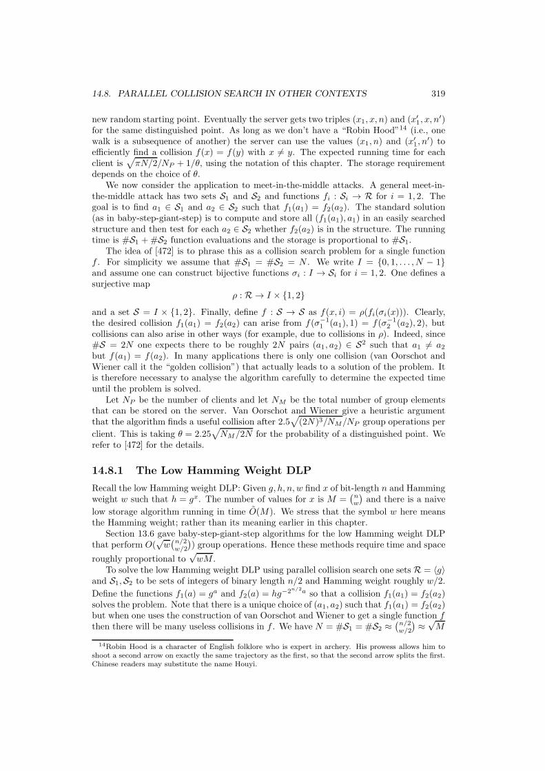
14.8. PARALLEL COLLISION SEARCH IN OTHER CONTEXTS 319

new random starting point. Eventually the server gets two triples (x1, x, n) and (x′1, x, n′)

for the same distinguished point. As long as we don’t have a “Robin Hood”14 (i.e., onewalk is a subsequence of another) the server can use the values (x1, n) and (x′1, n

′) toefficiently find a collision f(x) = f(y) with x 6= y. The expected running time for eachclient is

√

πN/2/NP + 1/θ, using the notation of this chapter. The storage requirementdepends on the choice of θ.

We now consider the application to meet-in-the-middle attacks. A general meet-in-the-middle attack has two sets S1 and S2 and functions fi : Si → R for i = 1, 2. Thegoal is to find a1 ∈ S1 and a2 ∈ S2 such that f1(a1) = f2(a2). The standard solution(as in baby-step-giant-step) is to compute and store all (f1(a1), a1) in an easily searchedstructure and then test for each a2 ∈ S2 whether f2(a2) is in the structure. The runningtime is #S1 +#S2 function evaluations and the storage is proportional to #S1.

The idea of [472] is to phrase this as a collision search problem for a single functionf . For simplicity we assume that #S1 = #S2 = N . We write I = {0, 1, . . . , N − 1}and assume one can construct bijective functions σi : I → Si for i = 1, 2. One defines asurjective map

ρ : R → I × {1, 2}and a set S = I × {1, 2}. Finally, define f : S → S as f(x, i) = ρ(fi(σi(x))). Clearly,the desired collision f1(a1) = f2(a2) can arise from f(σ−1

1 (a1), 1) = f(σ−12 (a2), 2), but

collisions can also arise in other ways (for example, due to collisions in ρ). Indeed, since#S = 2N one expects there to be roughly 2N pairs (a1, a2) ∈ S2 such that a1 6= a2but f(a1) = f(a2). In many applications there is only one collision (van Oorschot andWiener call it the “golden collision”) that actually leads to a solution of the problem. Itis therefore necessary to analyse the algorithm carefully to determine the expected timeuntil the problem is solved.

Let NP be the number of clients and let NM be the total number of group elementsthat can be stored on the server. Van Oorschot and Wiener give a heuristic argumentthat the algorithm finds a useful collision after 2.5

√

(2N)3/NM/NP group operations per

client. This is taking θ = 2.25√

NM/2N for the probability of a distinguished point. Werefer to [472] for the details.

14.8.1 The Low Hamming Weight DLP

Recall the low Hamming weight DLP: Given g, h, n, w find x of bit-length n and Hammingweight w such that h = gx. The number of values for x is M =

(

nw

)

and there is a naive

low storage algorithm running in time O(M). We stress that the symbol w here meansthe Hamming weight; rather than its meaning earlier in this chapter.

Section 13.6 gave baby-step-giant-step algorithms for the low Hamming weight DLPthat perform O(

√w(n/2w/2

)

) group operations. Hence these methods require time and space

roughly proportional to√wM .

To solve the low Hamming weight DLP using parallel collision search one sets R = 〈g〉and S1,S2 to be sets of integers of binary length n/2 and Hamming weight roughly w/2.

Define the functions f1(a) = ga and f2(a) = hg−2n/2a so that a collision f1(a1) = f2(a2)solves the problem. Note that there is a unique choice of (a1, a2) such that f1(a1) = f2(a2)but when one uses the construction of van Oorschot and Wiener to get a single function fthen there will be many useless collisions in f . We have N = #S1 = #S2 ≈

(n/2w/2

)

≈√M

14Robin Hood is a character of English folklore who is expert in archery. His prowess allows him toshoot a second arrow on exactly the same trajectory as the first, so that the second arrow splits the first.Chinese readers may substitute the name Houyi.


and so get an algorithm whose number of group operations is proportional toN3/2 =M3/4

yet requires low storage. This is a significant improvement over the naive low-storagemethod, but still slower than baby-step-giant-step.

Exercise 14.8.1. Write this algorithm in pseudocode and give a more careful analysisof the running time.

It remains an open problem to give a low memory algorithm for the low Hammingweight DLP with complexity proportional to

√wM as with the BSGS methods.

14.9 Pollard Rho Factoring Method

This algorithm was proposed in [485] and was the first algorithm invented by Pollard thatexploited pseudorandom walks. As more powerful factoring algorithms exist, we keep thepresentation brief. For further details see Section 5.6.2 of Stinson [591] or Section 5.2.1of Crandall and Pomerance [161].

Let N be a composite integer to be factored and let p | N be a prime (usually p isthe smallest prime divisor of N). We try to find a relation that holds modulo p but notmodulo other primes dividing N .

The basic idea of the rho factoring algorithm is to consider the pseudorandom walkx1 = 2 and

xi+1 = f(xi) (mod N)

where the usual choice for f(x) is x2 + 1 (or f(x) = x2 + a for some small integer a).Consider the values xi (mod p) where p | N . The sequence xi (mod p) is a pseudorandomsequence of residues modulo p, and so after about

√

πp/2 steps we expect there to beindicies i and j such that xi ≡ xj (mod p). We call this a collision. If xi 6≡ xj (mod N)then we can split N as gcd(xi − xj , N).

Example 14.9.1. Let p = 11. Then the rho iteration modulo p is

2, 5, 4, 6, 4, 6, 4, . . .

Let p = 19. Then the sequence is

2, 5, 7, 12, 12, 12, . . .

As with the discrete logarithm algorithms, the walk is deterministic in the sense thata collision leads to a cycle. Let lt be the length of the tail and lh be the length of thecycle. Then the first collision is

xlt+lh ≡ xlt (mod p).

We can use Floyd’s cycle finding algorithm to detect the collision. The details are givenin Algorithm 21. Note that it is not efficient to compute the gcd in line 5 of the algorithmfor each iteration; Pollard [485] gave a solution to reduce the number of gcd computationsand Brent [98] gave another.

We now briefly discuss the complexity of the algorithm. Note that the “algorithm”may not terminate, for example if the length of the cycle and tail are the same for allp | N then the gcd will always be either 1 or N . In practice one would stop the algorithmafter a certain number of steps and repeat with a different choice of x1 and/or f(x). Evenif it terminates, the length of the cycle of the rho may be very large. Hence, the usualapproach is to make the heuristic assumption that the rho pseudorandom walk behaves

14.9. POLLARD RHO FACTORING METHOD 321

Algorithm 21 The rho algorithm for factoring

Input: NOutput: A factor of N1: x1 = 2, x2 = f(x1) (mod N)2: repeat

3: x1 = f(x1) (mod N)4: x2 = f(f(x2)) (mod N)5: d = gcd(x2 − x1, N)6: until 1 < d < N7: return d

like a random walk. To have meaningful heuristics one should analyse the algorithm whenthe function f(x) is randomly chosen from a large set of possible functions.

Note that the rho method is more general than the p − 1 method (see Section 12.3),since a random p | N is not very likely to be

√p-smooth.

Theorem 14.9.2. Let N be composite, not a prime power and not “too smooth”. Assumethat the Pollard rho walk modulo p behaves like a pseudorandom walk for all p | N . Thenthe rho algorithm factors N in O(N1/4 log(N)2) bit operations.

Proof: (Sketch) Let p be a prime dividing N such that p ≤√N . Define the values lt

and lh corresponding to the sequence xi (mod p). If the walk behaves sufficiently like arandom walk then, by the birthday paradox, we will have lh, lt ≈

√

πp/8. Similarly, forsome other prime q | N one expects that the walk modulo q has different values lh andlt. Hence, after O(

√p) iterations of the loop one expects to split N . �

Bach [21] has given a rigorous analysis of the rho factoring algorithm. He provesthat if 0 ≤ x, y < N are chosen randomly and the iteration is x1 = x, xi+1 = x2i + y,then the probability of finding the smallest prime factor p of N after k steps is at leastk(k − 1)/2p+O(p−3/2) as p goes to infinity, where the constant in the O depends on k.Bach’s method cannot be used to analyse the rho algorithm for discrete logarithms.

Example 14.9.3. Let N = 144493. The values (xi, x2i) for i = 1, 2, . . . , 7 are

(2, 5), (5, 677), (26, 9120), (677, 81496), (24851, 144003), (9120, 117992), (90926, 94594)

and one can check that gcd(x14 − x7, N) = 131.The reason for this can be seen by considering the values xi modulo p = 131. The

sequence of values starts

2, 5, 26, 22, 92, 81, 12, 14, 66, 34, 109, 92

and we see that x12 = x5 = 92. The tail has length lt = 5 and the head has length lh = 7.Clearly, x14 ≡ x7 (mod p).

Exercise 14.9.4. Factor the number 576229 using the rho algorithm.

Exercise 14.9.5. The rho algorithm usually uses the function f(x) = x2 + 1. Why doyou think this function is used? Why are the functions f(x) = x2 and f(x) = x2 − 2 lesssuitable?

Exercise 14.9.6. Show that if N is known to have a prime factor p ≡ 1 (mod m) form > 2 then it is preferable to use the polynomial f(x) = xm + 1.


Exercise 14.9.7. Floyd’s and Brent’s cycle finding methods are both useful for therho factoring algorithm. Explain why one cannot use the other cycle finding meth-ods listed in Section 14.2.2 (Sedgewick-Szymanski-Yao, Schnorr-Lenstra, Nivasch, dis-tinguished points) for the rho factoring method.

14.10 Pollard Kangaroo Factoring

One can also use the kangaroo method to obtain a factoring algorithm. This is a muchmore direct application of the discrete logarithm algorithm we have already presented.Let N = pq be a product of two n-bit primes. Then

√N < p+ q < 3

√N . Let g ∈ Z

∗N be

chosen at random. Since gϕ(N)/2 ≡ 1 (mod N) we have

g(N+1)/2 ≡ gx (mod N)

for x = (p+ q)/2. In other words, we have a discrete logarithm problem in Z∗N an interval

of width√N . Using the standard kangaroo algorithm in the group Z

∗N one expects to

find x (and hence split N) in time O(N1/4).

Exercise 14.10.1. The above analysis was for integers N which are a product of twoprimes of very similar size. Let N now be a general composite integer and let p | N bethe smallest prime dividing N . Then p <

√N . Choose g ∈ Z

∗N and let h = gN (mod N).

Then h ≡ gx (mod p) for some 1 ≤ x < p. It is natural to try to use the kangaroo methodto find x in time O(

√p log(N)2). If x were found then gN−x ≡ 1 (mod p) and so one can

split N as gcd(gN−x − 1 (mod N), N). However, it seems to be impossible to constructan algorithm based on this idea. Explain why.

Factoring and Discrete Logarithms using PseudorandomWalkssgal018/crypto-book/ch14.pdf · Factoring...

Documents

Transcript of Factoring and Discrete Logarithms using PseudorandomWalkssgal018/crypto-book/ch14.pdf · Factoring...