Factorial ANOVA More than one categorical explanatory variable STA305 Spring 2014.
37
Factorial ANOVA More than one categorical explanatory variable STA305 Spring 2014 See last slide for copyright information
-
Upload
scott-davis -
Category
Documents
-
view
226 -
download
0
Transcript of Factorial ANOVA More than one categorical explanatory variable STA305 Spring 2014.
Factorial ANOVA
More than one categorical explanatory variable
STA305 Spring 2014
See last slide for copyright information

2
Optional Background Reading
• Chapter 7 of Data analysis with SAS
3
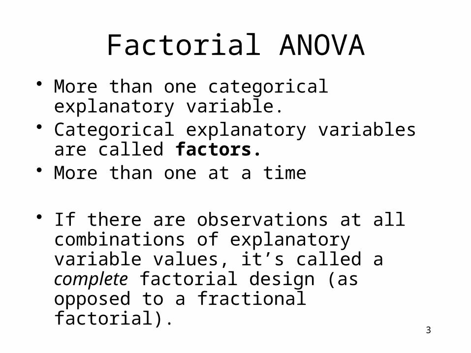
Factorial ANOVA• More than one categorical explanatory
variable.• Categorical explanatory variables are called
factors.• More than one at a time
• If there are observations at all combinations of explanatory variable values, it’s called a complete factorial design (as opposed to a fractional factorial).
4
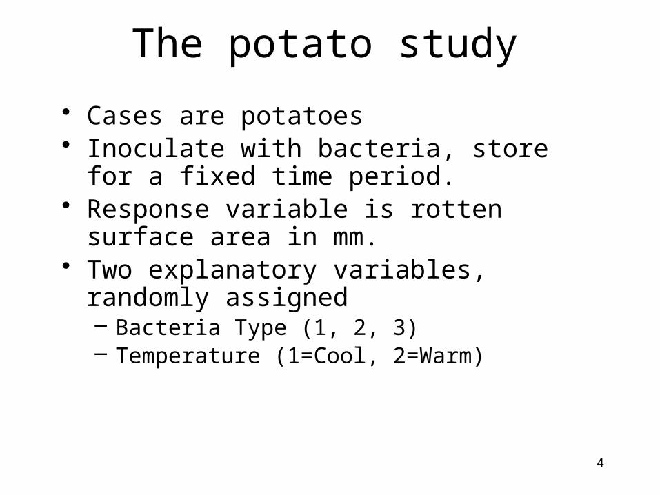
The potato study
• Cases are potatoes• Inoculate with bacteria, store for a fixed time
period.• Response variable is rotten surface area in
mm.• Two explanatory variables, randomly
assigned– Bacteria Type (1, 2, 3)– Temperature (1=Cool, 2=Warm)

5
Two-factor design
Bacteria TypeTemp 1 2 3
1=Cool
2=Warm
Six treatment conditions

6
Factorial experiments
• Allow more than one factor to be investigated in the same study: Efficiency!
• Allow the scientist to see whether the effect of an explanatory variable depends on the value of another explanatory variable: Interactions
• Thank you again, Mr. Fisher.

7
Normal with equal variance and conditional (cell) means
Bacteria TypeTemp 1 2 3
1=Cool
2=Warm
8
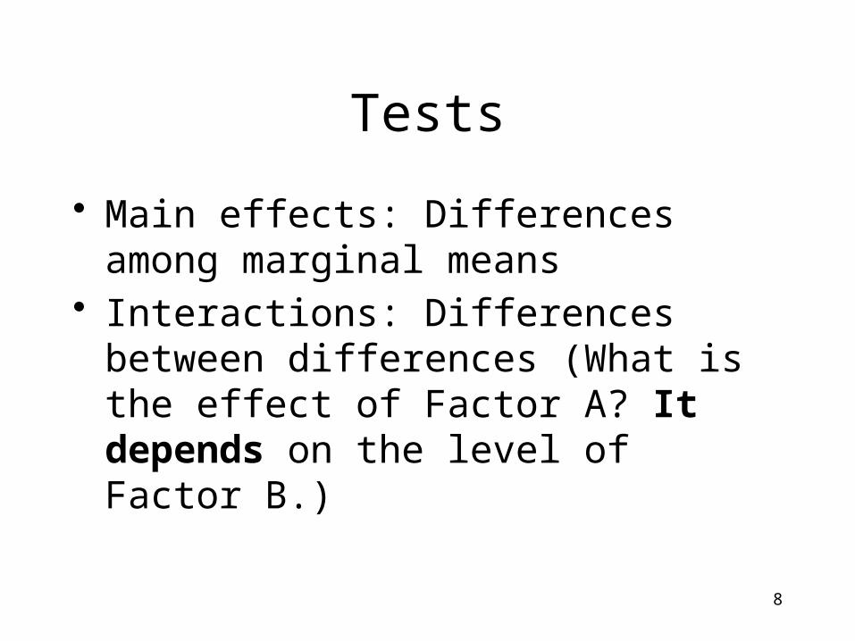
Tests
• Main effects: Differences among marginal means
• Interactions: Differences between differences (What is the effect of Factor A? It depends on the level of Factor B.)
9
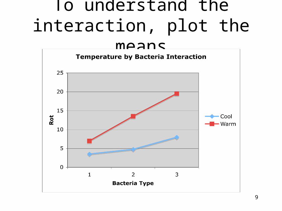
To understand the interaction, plot the means

10
Either Way
11
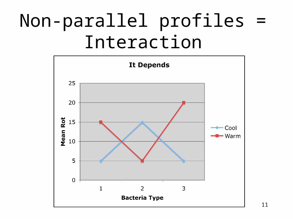
Non-parallel profiles = Interaction
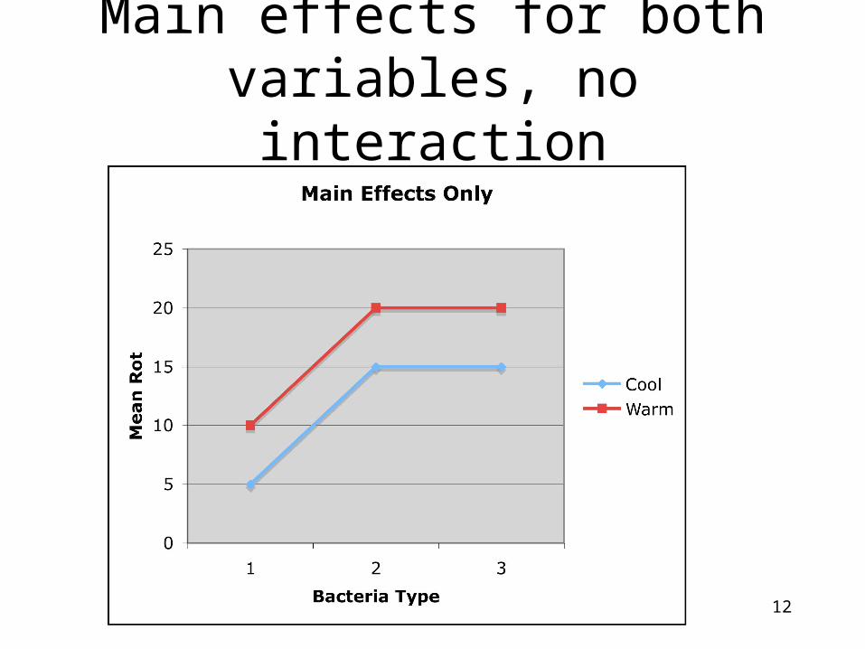
12
Main effects for both variables, no interaction
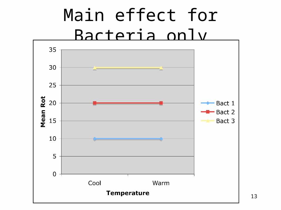
13
Main effect for Bacteria only

14
Main Effect for Temperature Only

15
Both Main Effects, and the Interaction

16
Should you interpret the main effects?

17
Testing Contrasts
• Differences between marginal means are definitely contrasts
• Interactions are also sets of contrasts

18
Interactions are sets of Contrasts
•
•
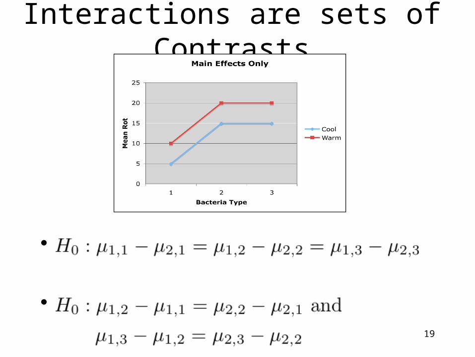
19
Interactions are sets of Contrasts
•
•
20
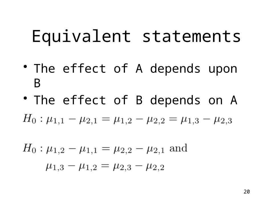
Equivalent statements
• The effect of A depends upon B• The effect of B depends on A

21
Three factors: A, B and C
• There are three (sets of) main effects: One each for A, B, C
• There are three two-factor interactions– A by B (Averaging over C)– A by C (Averaging over B)– B by C (Averaging over A)
• There is one three-factor interaction: AxBxC
22
Meaning of the 3-factor interaction
• The form of the A x B interaction depends on the value of C
• The form of the A x C interaction depends on the value of B
• The form of the B x C interaction depends on the value of A
• These statements are equivalent. Use the one that is easiest to understand.
23
To graph a three-factor interaction
• Make a separate mean plot (showing a 2-factor interaction) for each value of the third variable.
• In the potato study, a graph for each type of potato
24
Four-factor design
• Four sets of main effects• Six two-factor interactions• Four three-factor interactions• One four-factor interaction: The nature
of the three-factor interaction depends on the value of the 4th factor
• There is an F test for each one• And so on …
25
As the number of factors increases
• The higher-way interactions get harder and harder to understand
• All the tests are still tests of sets of contrasts (differences between differences of differences …)
• But it gets harder and harder to write down the contrasts
• Effect coding becomes easier

26
Effect coding
Bact B1 B2
1 1 0
2 0 1
3 -1 -1
Temperature T
1=Cool 1
2=Warm -1

27
Interaction effects are products of dummy variables
• The A x B interaction: Multiply each dummy variable for A by each dummy variable for B
• Use these products as additional explanatory variables in the multiple regression
• The A x B x C interaction: Multiply each dummy variable for C by each product term from the A x B interaction
• Test the sets of product terms simultaneously
28
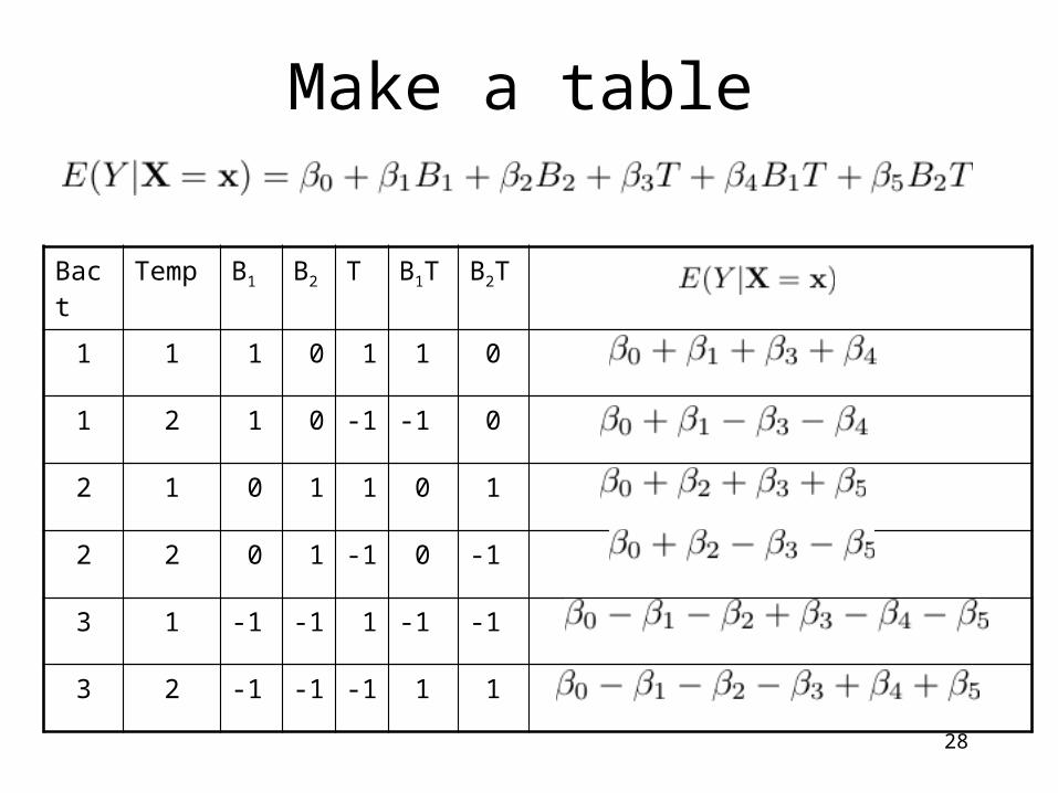
Make a table
Bact Temp B1 B2 T B1T B2T
1 1 1 0 1 1 0
1 2 1 0 -1 -1 0
2 1 0 1 1 0 1
2 2 0 1 -1 0 -1
3 1 -1 -1 1 -1 -1
3 2 -1 -1 -1 1 1
29
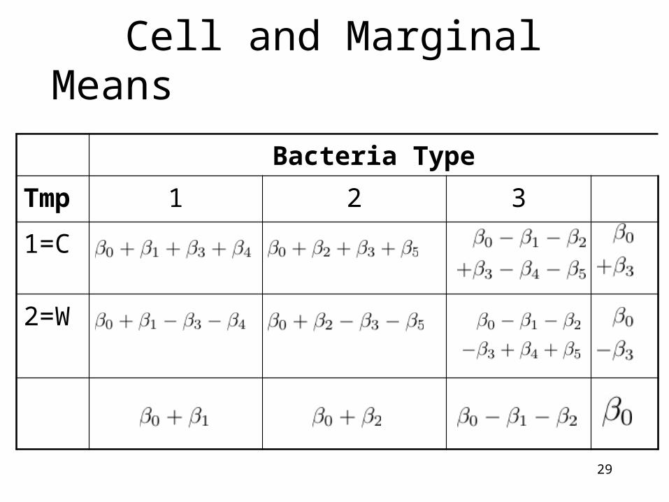
Cell and Marginal Means
Bacteria TypeTmp 1 2 3
1=C
2=W

30
We see
• Intercept is the grand mean• Regression coefficients for the dummy
variables are deviations of the marginal means from the grand mean
• What about the interactions?
31
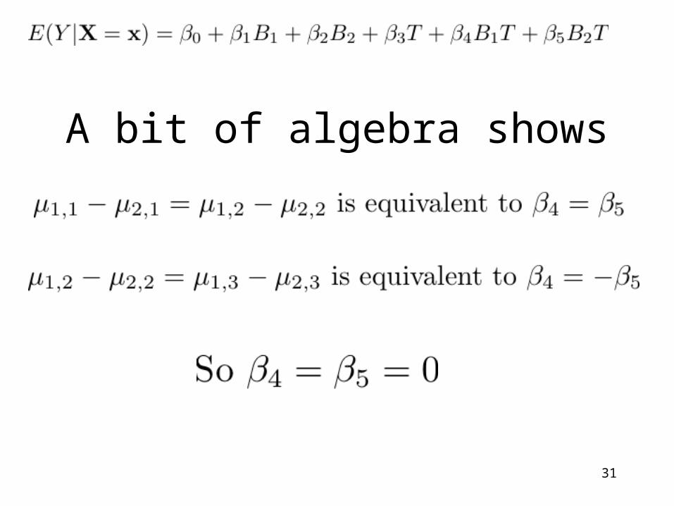
A bit of algebra shows

32
Factorial ANOVA with effect coding is pretty automatic
• You don’t have to make a table unless asked.• It always works as you expect it will.• Hypothesis tests are the same as testing sets
of contrasts.
33
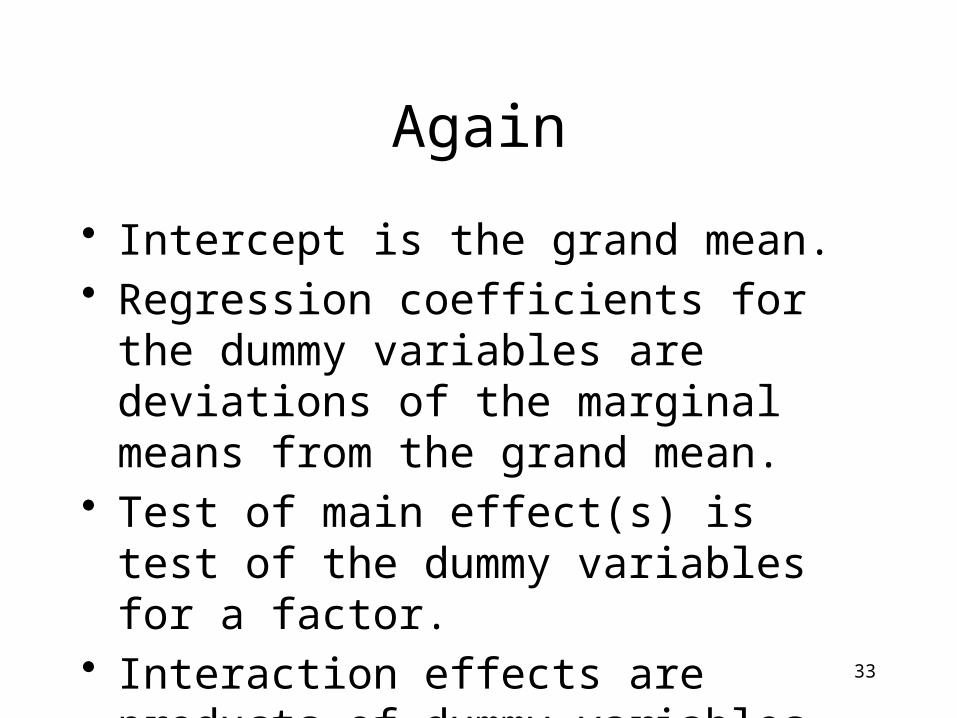
Again
• Intercept is the grand mean.• Regression coefficients for the dummy
variables are deviations of the marginal means from the grand mean.
• Test of main effect(s) is test of the dummy variables for a factor.
• Interaction effects are products of dummy variables.
34
Balanced vs. Unbalanced Experimental Designs
• Balanced design: Cell sample sizes are proportional (maybe equal).
• Explanatory variables have zero relationship to one another.
• Numerator SS in ANOVA are independent (because contrasts are orthogonal).
• Everything is nice and simple• Most experimental studies are designed this
way.• As soon as somebody drops a test tube, it’s
no longer balanced.
35
Analysis of unbalanced data
• When explanatory variables are related, there is potential ambiguity.
• A is related to Y, B is related to Y, and A is related to B.
• Who gets credit for the portion of variation in Y that could be explained by either A or B?
• With a regression approach, whether you use contrasts or dummy variables (equivalent), the answer is nobody.
• Think of full, reduced models.• Equivalently, general linear test

36
Some software is designed for balanced data
• The special purpose formulas are much simpler.• Very useful in the past.• Since most data are at least a little unbalanced, a
recipe for trouble.• Most textbook data are balanced, so they cannot tell
you what your software is really doing.• R’s anova and aov functions are designed for
balanced data, though anova applied to lm objects can give you what you want if you use it with care.
• SAS proc glm is much more convenient. SAS proc anova is for balanced data.

37
Copyright Information
This slide show was prepared by Jerry Brunner, Department of
Statistics, University of Toronto. It is licensed under a Creative
Commons Attribution - ShareAlike 3.0 Unported License. Use
any part of it as you like and share the result freely. These
PowerPoint slides will be available from the course website:
http://www.utstat.toronto.edu/brunner/oldclass/305s14