Factor graphs and the sum-product algorithm - Information ... · Factor Graphs and the Sum-Product...

498 IEEE TRANSACTIONS ON INFORMATION THEORY, VOL. 47, NO. 2, FEBRUARY 2001

Factor Graphs and the Sum-Product AlgorithmFrank R. Kschischang, Senior Member, IEEE, Brendan J. Frey, Member, IEEE, and

Hans-Andrea Loeliger, Member, IEEE

Abstract—Algorithms that must deal with complicated globalfunctions of many variables often exploit the manner in which thegiven functions factor as a product of “local” functions, each ofwhich depends on a subset of the variables. Such a factorizationcan be visualized with a bipartite graph that we call afactor graph.In this tutorial paper, we present a generic message-passing algo-rithm, the sum-product algorithm, that operates in a factor graph.Following a single, simple computational rule, the sum-productalgorithm computes—either exactly or approximately—var-ious marginal functions derived from the global function. Awide variety of algorithms developed in artificial intelligence,signal processing, and digital communications can be derived asspecific instances of the sum-product algorithm, including theforward/backward algorithm, the Viterbi algorithm, the iterative“turbo” decoding algorithm, Pearl’s belief propagation algorithmfor Bayesian networks, the Kalman filter, and certain fast Fouriertransform (FFT) algorithms.

Index Terms—Belief propagation, factor graphs, fast Fouriertransform, forward/backward algorithm, graphical models, iter-ative decoding, Kalman filtering, marginalization, sum-productalgorithm, Tanner graphs, Viterbi algorithm.

I. INTRODUCTION

T HIS paper provides a tutorial introduction to factor graphsand the sum-product algorithm, a simple way to under-

stand a large number of seemingly different algorithms that havebeen developed in computer science and engineering. We con-sider algorithms that deal with complicated “global” functionsof many variables and that derive their computational efficiencyby exploiting the way in which the global function factors intoa product of simpler “local” functions, each of which dependson a subset of the variables. Such a factorization can be visual-ized using afactor graph, a bipartite graph that expresses whichvariables are arguments of which local functions.

Manuscript received August 3, 1998; revised October 17, 2000. The workof F. R. Kschischang was supported in part, while on leave at the Massachu-setts Institute of Technology, by the Office of Naval Research under GrantN00014-96-1-0930, and by the Army Research Laboratory under CooperativeAgreement DAAL01-96-2-0002. The work of B. J. Frey was supported,while a Beckman Fellow at the Beckman Institute of Advanced Science andTechnology, University of Illinois at Urbana-Champaign, by a grant fromthe Arnold and Mabel Beckman Foundation. The material in this paper waspresented in part at the 35th Annual Allerton Conference on Communication,Control, and Computing, Monticello, IL, September 1997.

F. R. Kschischang is with the Department of Electrical and ComputerEngineering, University of Toronto, Toronto, ON M5S 3G4, Canada (e-mail:[email protected]).

B. J. Frey is with the Faculty of Computer Science, University of Waterloo,Waterloo, ON N2L 3G1, Canada, and the Faculty of Electrical and Com-puter Engineering, University of Illinois at Urbana-Champaign, Urbana, IL61801-2307 USA (e-mail: [email protected]).

H.-A. Loeliger is with the Signal Processing Lab (ISI), ETH Zentrum,CH-8092 Zürich, Switzerland (e-mail: [email protected]).

Communicated by T. E. Fuja, Associate Editor At Large.Publisher Item Identifier S 0018-9448(01)00721-0.

The aim of this tutorial paper is to introduce factor graphsand to describe a generic message-passing algorithm, called thesum-product algorithm, which operates in a factor graph and at-tempts to compute various marginal functions associated withthe global function. The basic ideas are very simple; yet, aswe will show, a surprisingly wide variety of algorithms devel-oped in the artificial intelligence, signal processing, and dig-ital communications communities may be derived as specificinstances of the sum-product algorithm, operating in an appro-priately chosen factor graph.

Genealogically, factor graphs are a straightforward gen-eralization of the “Tanner graphs” of Wiberget al. [31],[32]. Tanner [29] introduced bipartite graphs to describefamilies of codes which are generalizations of the low-densityparity-check (LDPC) codes of Gallager [11], and also describedthe sum-product algorithm in this setting. In Tanner’s originalformulation, all variables are codeword symbols and hence“visible”; Wiberg et al., introduced “hidden” (latent) state vari-ables and also suggested applications beyond coding. Factorgraphs take these graph-theoretic models one step further, byapplying them to functions. From the factor-graph perspective(as we will describe in Section III-A), a Tanner graph for acode represents a particular factorization of the characteristic(indicator) function of the code.

While it may seem intuitively reasonable that some algo-rithms should exploit the manner in which a global functionfactors into a product of local functions, the fundamental insightthat many well-known algorithms essentially solve the “MPF”(marginalize product-of-functions) problem, each in their ownparticular setting, was first made explicit in the work of Ajiand McEliece [1]. In a landmark paper [2], Aji and McEliecedevelop a “generalized distributive law” (GDL) that in somecases solves the MPF problem using a “junction tree” represen-tation of the global function. Factor graphs may be viewed asan alternative approach with closer ties to Tanner graphs andpreviously developed graphical representations for codes. Es-sentially, every result developed in the junction tree/GDL set-ting may be translated into an equivalent result in the factorgraph/sum-product algorithm setting, andvice versa. We preferthe latter setting not only because it is better connected with pre-vious approaches, but also because we feel that factor graphs arein some ways easier to describe, giving them a modest pedagog-ical advantage. Moreover, the sum-product algorithm can oftenbe applied successfully in situations where exact solutions to theMPF problem (as provided by junction trees) become computa-tionally intractable, the most prominent example being the iter-ative decoding of turbo codes and LDPC codes. In Section VIwe do, however, discuss strategies for achieving exact solutionsto the MPF problem in factor graphs.

0018–9448/01$10.00 © 2001 IEEE

KSCHISCHANGet al.: FACTOR GRAPHS AND THE SUM-PRODUCT ALGORITHM 499

There are also close connections between factor graphs andgraphical representations (graphical models) for multidimen-sional probability distributions such as Markov random fields[16], [18], [26] and Bayesian (belief) networks [25], [17]. Likefactor graphs, these graphical models encode in their structure aparticular factorization of the joint probability mass function ofseveral random variables. Pearl’s powerful “belief propagation”algorithm [25], which operates by “message-passing” in aBayesian network, translates immediately into an instance ofthe sum-product algorithm operating in a factor graph thatexpresses the same factorization. Bayesian networks and beliefpropagation have been used previously to explain the iterativedecoding of turbo codes and LDPC codes [9], [10], [19], [21],[22], [24], the most powerful practically decodable codesknown. Note, however, that Wiberg [31] had earlier describedthese decoding algorithms as instances of the sum-productalgorithm; see also [7].

We begin the paper in Section II with a small worked examplethat illustrates the operation of the sum-product algorithm in asimple factor graph. We will see that when a factor graph iscycle-free, then the structure of the factor graph not only en-codes the way in which a given function factors, but also en-codesexpressionsfor computing the various marginal functionsassociated with the given function. These expressions lead di-rectly to the sum-product algorithm.

In Section III, we show how factor graphs may be used as asystem and signal-modeling tool. We see that factor graphs arecompatible both with “behavioral” and “probabilistic” modelingstyles. Connections between factor graphs and other graphicalmodels are described briefly in Appendix B, where we recoverPearl’s belief propagation algorithm as an instance of the sum-product algorithm.

In Section IV, we apply the sum-product algorithm totrellis-structured (hidden Markov) models, and obtain theforward/backward algorithm, the Viterbi algorithm, and theKalman filter as instances of the sum-product algorithm. InSection V, we consider factor graphs with cycles, and obtainthe iterative algorithms used to decode turbo-like codes asinstances of the sum-product algorithm.

In Section VI, we describe several generic transformationsby which a factor graph with cycles may sometimes be con-verted—often at great expense in complexity—to an equivalentcycle-free form. We apply these ideas to the factor graph repre-senting the discrete Fourier transform (DFT) kernel, and derivea fast Fourier transform (FFT) algorithm as an instance of thesum-product algorithm.

Some concluding remarks are given in Section VII.

II. M ARGINAL FUNCTIONS, FACTOR GRAPHS, AND THE

SUM-PRODUCT ALGORITHM

Throughout this paper we deal with functions of many vari-ables. Let , be a collection of variables, in which,for each , takes on values in some (usually finite)domain(or alphabet) . Let be an -valued functionof these variables, i.e., a function with domain

and codomain . The domain of is called theconfigurationspacefor the given collection of variables, and each element of

is a particularconfigurationof the variables, i.e., an assign-ment of a value to each variable. The codomainof may ingeneral be any semiring [2], [31, Sec. 3.6]; however, at least ini-tially, we will lose nothing essential by assuming thatis theset of real numbers.

Assuming that summation in is well defined, then associ-ated with every function are marginal func-tions . For each , the value of is obtained bysumming the value of over all configurations ofthe variables that have .

This type of sum is so central to this paper that we introducea nonstandard notation to handle it: the “not-sum” orsummary.Instead of indicating the variables being summed over, we indi-cate those variablesnotbeing summed over. For example, ifisa function of three variables , , and , then the “summaryfor ” is denoted by

In this notation we have

i.e., the th marginal function associated with isthe summary for of .

We are interested in developing efficient procedures for com-puting marginal functions that a) exploit the way in which theglobal function factors, using the distributive law to simplify thesummations, and b) reuses intermediate values (partial sums).As we will see, such procedures can be expressed very natu-rally by use of a factor graph.

Suppose that factors into a product of severallocal functions, each having some subset of asarguments; i.e., suppose that

(1)

where is a discrete index set, is a subset of ,and is a function having the elements of as argu-ments.

Definition: A factor graphis a bipartite graph that expressesthe structure of the factorization (1). A factor graph has avari-able nodefor each variable , afactor nodefor each local func-tion , and an edge-connecting variable nodeto factor node

if and only if is an argument of .

A factor graph is thus a standard bipartite graphical represen-tation of a mathematical relation—in this case, the “is an argu-ment of” relation between variables and local functions.

Example 1 (A Simple Factor Graph):Letbe a function of five variables, and suppose thatcan

be expressed as a product

(2)


Fig. 1. A factor graph for the productf (x )f (x )f (x ; x ; x )� f (x ; x )f (x ; x ).

of five factors, so that , ,, , , and

. The factor graph that corresponds to (2) is shown inFig. 1.

A. Expression Trees

In many situations (for example, when rep-resents a joint probability mass function), we are interested incomputing the marginal functions . We can obtain an ex-pression for each marginal function by using (2) and exploitingthe distributive law.

To illustrate, we write from Example 1 as

or, in summary notation

(3)

Similarly, we find that

(4)

In computer science, arithmetic expressions like theright-hand sides of (3) and (4) are often represented by or-dered rooted trees [28, Sec. 8.3], here calledexpression trees,in which internal vertices (i.e., vertices with descendants)represent arithmetic operators (e.g., addition, multiplication,negation, etc.) and leaf vertices (i.e., vertices without descen-dants) represent variables or constants. For example, the tree ofFig. 2 represents the expression . When the operatorsin an expression tree are restricted to those that are completelysymmetric in their operands (e.g., multiplication and addition),

Fig. 2. An expression tree representingx(y + z).

it is unnecessary to order the vertices to avoid ambiguity ininterpreting the expression represented by the tree.

In this paper, we extend expression trees so that the leaf ver-tices representfunctions, not just variables or constants. Sumsand products in such expression trees combine their operands inthe usual (pointwise) manner in which functions are added andmultiplied. For example, Fig. 3(a) unambiguously represents theexpression on the right-hand side of (3), and Fig. 4(a) unambigu-ously represents the expression on the right-hand side of (4). Theoperators shown in these figures are the function product and thesummary, having various local functions as their arguments.

Also shown in Figs. 3(b) and 4(b), are redrawings of the factorgraph of Fig. 1 as a rooted tree with and as root vertex,respectively. This is possible because the global function de-fined in (2) was deliberately chosen so that the correspondingfactor graph is a tree. Comparing the factor graphs with the cor-responding trees representing the expression for the marginalfunction, it is easy to note their correspondence. This observa-tion is simple, but key:when a factor graph is cycle-free, thefactor graph not only encodes in its structure the factorizationof the global function, but also encodes arithmetic expressionsby which the marginal functions associated with the global func-tion may be computed.

Formally, as we show in Appendix A, to convert a cycle-freefactor graph representing a function to the cor-responding expression tree for , draw the factor graph asa rooted tree with as root. Every node in the factor graphthen has a clearly defined parent node, namely, the neighboringnode through which the unique path fromto must pass. Re-place each variable node in the factor graph with a product op-erator. Replace each factor node in the factor graph with a “formproduct and multiply by ” operator, and between a factor node

and its parent , insert a summary operator. Theselocal transformations are illustrated in Fig. 5(a) for a variablenode, and in Fig. 5(b) for a factor nodewith parent . Trivialproducts (those with one or no operand) act as identity opera-tors, or may be omitted if they are leaf nodes in the expressiontree. A summary operator applied to a function with asingle argument is also a trivial operation, and may be omitted.Applying this transformation to the tree of Fig. 3(b) yields theexpression tree of Fig. 3(a), and similarly for Fig. 4. Trivial op-erations are indicated with dashed lines in these figures.

B. Computing a Single Marginal Function

Every expression tree represents analgorithmfor computingthe corresponding expression. One might describe the algorithmas a recursive “top-down” procedure that starts at the root vertexand evaluates each subtree descending from the root, combiningthe results as dictated by the operator at the root. Equivalently,we prefer to describe the algorithm as a “bottom-up” procedurethat begins at the leaves of the tree, with each operator vertex


Fig. 3. (a) A tree representation for the right-hand side of (3). (b) The factor graph of Fig. 1, redrawn as a rooted tree withx as root.

Fig. 4. (a) A tree representation for the right-hand side of (4). (b) The factor graph of Fig. 1, redrawn as a rooted tree withx as root.

combining its operands and passing on the result as an operandfor its parent. For example, , represented by the ex-pression tree of Fig. 2, might be evaluated by starting at the leafnodes and , evaluating , and passing on the result as anoperand for the operator, which multiplies the result with.

Rather than working with the expression tree, it is simplerand more direct to describe such marginalization algorithms interms of the corresponding factor graph. To best understandsuch algorithms, it helps to imagine that there is a processorassociated with each vertex of the factor graph, and that thefactor-graph edges represent channels by which these proces-sors may communicate. For us, “messages” sent between pro-cessors are always simply some appropriate description of somemarginal function. (We describe some useful representations inSection V-E.)

We now describe a message-passing algorithm that we willtemporarily call the “single-sum-product algorithm,” since it

computes, for a single value of, the marginal functionin a rooted cycle-free factor graph, with taken as root vertex.

The computation begins at the leaves of the factor graph. Eachleaf variable node sends a trivial “identity function” message toits parent, and each leaf factor nodesends a description of

to its parent. Each vertex waits for messages from all of itschildren before computing the message to be sent to its parent.This computation is performed according to the transformationshown in Fig. 5; i.e., a variable node simply sends theproductof messages received from its children, while a factor nodewith parent forms the product of with the messages receivedfrom its children, and then operates on the result with asummary operator. By a “product of messages” we mean anappropriate description of the (pointwise) product of the cor-responding functions. If the messages are parametrizations ofthe functions, then the resulting message is the parametrizationof the product function, not (necessarily) literally the numerical


Fig. 5. Local substitutions that transform a rooted cycle-free factor graph toan expression tree for a marginal function at (a) a variable node and (b) a factornode.

product of the messages. Similarly, the summary operator is ap-plied to the functions, not necessarily literally to the messagesthemselves.

The computation terminates at the root node, where themarginal function is obtained as the product of all mes-sages received at .

It is important to note that a message passed on the edge, either from variable to factor , or vice versa, is a

single-argument function of, the variableassociated withthegiven edge. This follows since, at every factor node, summaryoperations are always performed for the variable associated withthe edge on which the message is passed. Likewise, at a variablenode, all messages are functions of that variable, and so is anyproduct of these messages.

The message passed on an edge during the operation of thesingle- sum-product algorithm can be interpreted as follows. If

is an edge in the tree, whereis a variable nodeand is a factor node, then the analysis of Appendix A showsthat the message passed onduring the operation of the sum-product algorithm is simply a summary forof theproduct ofthe local functionsdescending from the vertex that originatesthe message.

C. Computing All Marginal Functions

In many circumstances, we may be interested in computingfor more than one value of. Such a computation might

be accomplished by applying the single-algorithm separatelyfor each desired value of, but this approach is unlikely tobe efficient, since many of the subcomputations performed fordifferent values of will be the same. Computation offor all simultaneously can be efficiently accomplished by es-sentially “overlaying” on a single factor graph all possible in-stances of the single-algorithm. No particular vertex is takenas a root vertex, so there is no fixed parent/child relationshipamong neighboring vertices. Instead,eachneighbor of anygiven vertex is at some point regarded as a parent of. Themessage passed fromto is computed just as in the single-algorithm, i.e., as if were indeed the parent ofand all otherneighbors of were children.

As in the single- algorithm, message passing is initiated atthe leaves. Each vertexremains idle until messages have ar-rived on all but one of the edges incident on. Just as in the

Fig. 6. A factor-graph fragment, showing the update rules of the sum-productalgorithm.

single- algorithm, once these messages have arrived,is ableto compute a message to be sent on the one remaining edgeto its neighbor (temporarily regarded as the parent), just as inthe single- algorithm, i.e., according to Fig. 5. Let us denotethis temporary parent as vertex. After sending a message to

, vertex returns to the idle state, waiting for a “return mes-sage” to arrive from . Once this message has arrived, the vertexis able to compute and send messages to each of its neigh-bors (other than ), each being regarded, in turn, as a parent.The algorithm terminates once two messages have been passedover every edge, one in each direction. At variable node,the product of all incoming messages is the marginal function

, just as in the single-algorithm. Since this algorithm op-erates by computing various sums and products, we refer to itas thesum-productalgorithm.

The sum-product algorithm operates according to the fol-lowing simple rule:

The message sent from a nodeon an edge is theproduct of the local function at (or the unit functionif is a variable node) with all messages received aton edgesother than , summarized for the variableassociated with.

Let denote the message sent from nodeto nodein the operation of the sum-product algorithm, let

denote the message sent from nodeto node . Also, letdenote the set of neighbors of a given nodein a factor graph.Then, as illustrated in Fig. 6, the message computations per-formed by the sum-product algorithm may be expressed as fol-lows:

(5)

(6)

where is the set of arguments of the function.The update rule at a variable nodetakes on the particularly

simple form given by (5) because there is no local function toinclude, and the summary forof a product of functions of is


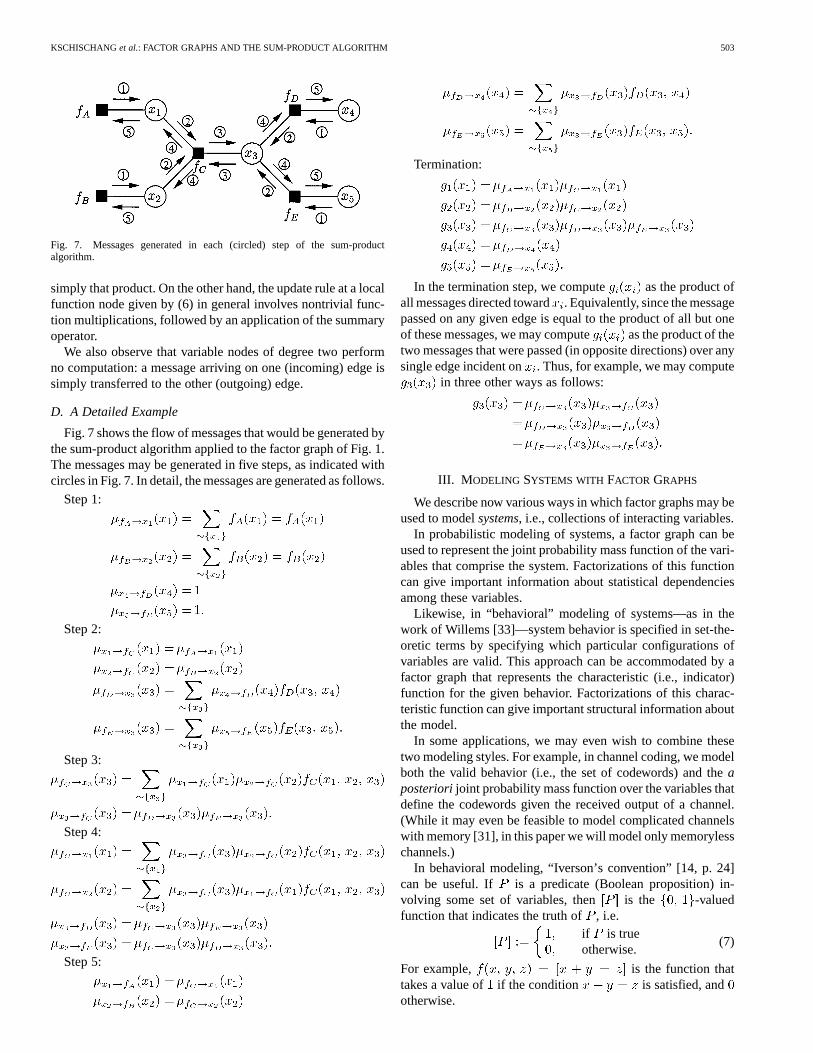
Fig. 7. Messages generated in each (circled) step of the sum-productalgorithm.

simply that product. On the other hand, the update rule at a localfunction node given by (6) in general involves nontrivial func-tion multiplications, followed by an application of the summaryoperator.

We also observe that variable nodes of degree two performno computation: a message arriving on one (incoming) edge issimply transferred to the other (outgoing) edge.

D. A Detailed Example

Fig. 7 shows the flow of messages that would be generated bythe sum-product algorithm applied to the factor graph of Fig. 1.The messages may be generated in five steps, as indicated withcircles in Fig. 7. In detail, the messages are generated as follows.

Step 1:

Step 2:

Step 3:

Step 4:

Step 5:

Termination:

In the termination step, we compute as the product ofall messages directed toward. Equivalently, since the messagepassed on any given edge is equal to the product of all but oneof these messages, we may compute as the product of thetwo messages that were passed (in opposite directions) over anysingle edge incident on . Thus, for example, we may compute

in three other ways as follows:

III. M ODELING SYSTEMS WITH FACTOR GRAPHS

We describe now various ways in which factor graphs may beused to modelsystems, i.e., collections of interacting variables.

In probabilistic modeling of systems, a factor graph can beused to represent the joint probability mass function of the vari-ables that comprise the system. Factorizations of this functioncan give important information about statistical dependenciesamong these variables.

Likewise, in “behavioral” modeling of systems—as in thework of Willems [33]—system behavior is specified in set-the-oretic terms by specifying which particular configurations ofvariables are valid. This approach can be accommodated by afactor graph that represents the characteristic (i.e., indicator)function for the given behavior. Factorizations of this charac-teristic function can give important structural information aboutthe model.

In some applications, we may even wish to combine thesetwo modeling styles. For example, in channel coding, we modelboth the valid behavior (i.e., the set of codewords) and theaposteriorijoint probability mass function over the variables thatdefine the codewords given the received output of a channel.(While it may even be feasible to model complicated channelswith memory [31], in this paper we will model only memorylesschannels.)

In behavioral modeling, “Iverson’s convention” [14, p. 24]can be useful. If is a predicate (Boolean proposition) in-volving some set of variables, then is the -valuedfunction that indicates the truth of, i.e.

if is trueotherwise.

(7)

For example, is the function thattakes a value of if the condition is satisfied, andotherwise.


If we let denote the logical conjunction or “AND” operator,then an important property of Iverson’s convention is that

(8)

(assuming and ). Thus, if can be writtenas a logical conjunction of predicates, then can be factoredaccording to (8), and hence represented by a factor graph.

A. Behavioral Modeling

Let be a collection of variables with config-uration space . By a behaviorin ,we mean any subset of . The elements of are thevalidconfigurations. Since a system is specified via its behavior,this approach is known as behavioral modeling [33].

Behavioral modeling is natural for codes. If the domain ofeach variable is some finite alphabet, so that the configurationspace is the -fold Cartesian product , then a behavior

is called ablock codeof length over , and the validconfigurations are calledcodewords.

The characteristic (or set membership indicator) function fora behavior is defined as

Obviously, specifying is equivalent to specifying . (Wemight also give a probabilistic interpretation by noting that

is proportional to a probability mass function that is uniformover the valid configurations.)

In many important cases, membership of a particular config-uration in a behavior can be determined by applying a seriesof tests (checks), each involving some subset of the variables.A configuration is deemed valid if and only if it passes all tests;i.e., the predicate may be written as a logicalconjunction of a series of “simpler” predicates. Thenfactorsaccording to (8) into a product of characteristic functions, eachindicating whether a particular subset of variables is an elementof some “local behavior.”

Example 2 (Tanner Graphs for Linear Codes):The char-acteristic function for any linear code defined by an parity-check matrix can be represented by a factor graph havingvariable nodes and factor nodes. For example, if is the bi-nary linear code with parity-check matrix

(9)

then is the set of all binary -tuplesthat satisfy three simultaneous equations expressed in matrixform as . (This is a so-calledkernel representation,since the linear code is defined as the kernel of a particular lineartransformation.) Membership in is completely determined bychecking whethereachof the three equations is satisfied. There-fore, using (8) and (9) we have

Fig. 8. A Tanner graph for the binary linear code of Example 2.

where denotes the sum in GF . The corresponding factorgraph is shown in Fig. 8, where we have used a special symbolfor the parity checks (a square with a “” sign). Althoughstrictly speaking the factor graph represents the factorizationof the code’s characteristic function, we will often refer to thefactor graph as representing the code itself. A factor graphobtained in this way is often called aTanner graph, after [29].

It should be obvious that a Tanner graph for any linearblock code may be obtained from a parity-check matrix

for the code. Such a parity-check matrix hascolumns andat least rows. Variable nodes correspond to the columnsof and factor nodes (or checks) to the rows of, with anedge-connecting factor nodeto variable node if and only if

. Of course, since there are, in general, many parity-check matrices that represent a given code, there are, in general,many Tanner graph representations for the code.

Given a collection of general nonlinear local checks, it may bea computationally intractable problem to determine whether thecorresponding behavior is nonempty. For example, the canon-ical NP-complete problemSAT (Boolean satisfiability) [13] issimply the problem of determining whether or not a collectionof Boolean variables satisfies all clauses in a given set. In effect,each clause is a local check.

Often, a description of a system is simplified by introducinghidden(sometimes called auxiliary, latent, or state) variables.Nonhidden variables are calledvisible. A particular behaviorwith both auxiliary and visible variables is said to represent agiven (visible) behavior if the projection of the elements of

on the visible variables is equal to. Any factor graph foris then considered to be also a factor graph for. Such graphswere introduced by Wiberget al. [31], [32] and may be calledWiberg-type graphs. In our factor graph diagrams, as in Wiberg,hidden variable nodes are indicated by a double circle.

An important class of models with hidden variables are thetrellis representations (see [30] for an excellent survey). A trellisfor a block code is an edge-labeled directed graph with distin-guished root and goal vertices, essentially defined by the prop-erty that each sequence of edge labels encountered in any di-rected path from the root vertex to the goal vertex is a codewordin , and that each codeword inis represented by at least onesuch path. Trellises also have the property that all paths fromthe root to any given vertex should have the same fixed length, called thedepthof the given vertex. The root vertex has depth, and the goal vertex has depth. The set of depth vertices

can be viewed as the domain of astate variable . For example,


Fig. 9. (a) A trellis and (b) the corresponding Wiberg-type graph for the code of Fig. 8.

Fig. 9(a) is a trellis for the code of Example 2. Vertices at thesame depth are grouped vertically. The root vertex is leftmost,the goal vertex is rightmost, and edges are implicitly directedfrom left to right.

A trellis divides naturally into sections, where theth trellissection is the subgraph of the trellis induced by the verticesat depth and depth . The set of edge labels in may beviewed as the domain of a (visible) variable. In effect, eachtrellis section defines a “local behavior” that constrains thepossible combinations of , , and .

Globally, a trellis defines a behavior in the configurationspace of the variables . A configu-ration of these variables is valid if and only if it satisfies thelocal constraints imposed by each of the trellis sections. Thecharacteristic function for this behavior thus factors naturallyinto factors, where theth factor corresponds to theth trellissection and has , , and as its arguments.

The following example illustrates these concepts in detail forthe code of Example 2.

Example 3 (A Trellis Description):Fig. 9(a) shows atrellis for the code of Example 2, and Fig. 9(b) shows thecorresponding Wiberg-type graph. In addition to the visiblevariable nodes , there are also hidden (state)variable nodes . Each local check, shown as ageneric factor node (black square), corresponds to one sectionof the trellis.

In this example, the local behavior corresponding to thesecond trellis section from the left in Fig. 9 consists of the fol-lowing triples :

(10)

where the domains of the state variablesand are taken tobe and , respectively, numbered from bottomto top in Fig. 9(a). Each element of the local behavior corre-sponds to one trellis edge. The corresponding factor node inthe Wiberg-type graph is the indicator function

.

It is important to note that a factor graph corresponding toa trellis is cycle-free. Since every code has a trellis representa-

Fig. 10. Generic factor graph for a state-space model of a time-invariant ortime-varying system.

tion, it follows that every code can be represented by a cycle-freefactor graph. Unfortunately, it often turns out that the state-spacesizes (the sizes of domains of the state variables) can easily be-come too large to be practical. For example, trellis representa-tions of turbo codes have enormous state spaces [12]. However,such codes may well have factor graph representations with rea-sonable complexities, but necessarily with cycles. Indeed, the“cut-set bound” of [31] (see also [8]) strongly motivates thestudy of graph representations with cycles.

Trellises are basically conventional state-space systemmodels, and the generic factor graph of Fig. 10 can representany state-space model of a time-invariant or time-varyingsystem. As in Fig. 9, each local check represents a trellissection; i.e., each check is an indicator function for the set ofallowed combinations of left (previous) state, input symbol,output symbol, and right (next) state. (Here, we allow a trellisedge to have both an input label and an output label.)

Example 4 (State-Space Models):For example, theclassical linear time-invariant state-space model is given by theequations

(11)

where is the discrete time index,are the time- input variables,

are the time- output variables, arethe time- state variables, , , , and are matrices of ap-propriate dimension, and the equations are over some field.


Any such system gives rise to the factor graph of Fig. 10. Thetime- check function

is

In other words, the check function enforces the local behaviordefined by (11).

B. Probabilistic Modeling

We turn now to another important class of functions that wewill represent by factor graphs: probability distributions. Sinceconditional and unconditional independence of random vari-ables is expressed in terms of a factorization of their joint prob-ability mass or density function, factor graphs for probabilitydistributions arise in many situations. We begin again with anexample from coding theory.

Example 5 (APP Distributions):Consider the standardcoding model in which a codeword isselected from a code of length and transmitted over amemoryless channel with corresponding output sequence

. For each fixed observation, the jointa posteriori probability (APP) distribution for the com-ponents of (i.e., ) is proportional to the function

, where is the a priori distributionfor the transmitted vectors, and is the conditionalprobability density function for when is transmitted.

Since the observed sequenceis fixed for any instance of“decoding” a graph we may consider to be a function ofonly, with the components ofregarded as parameters. In otherwords, we may write or as , meaning thatthe expression to be “decoded” always has the same parametricform, but that the parameter will in general be different indifferent decoding instances.

Assuming that thea priori distribution for the transmittedvectors is uniform over codewords, we have ,where is the characteristic function for and is thenumber of codewords in . If the channel is memoryless, then

factors as

Under these assumptions, we have

(12)

Now the characteristic function itself may factor into aproduct of local characteristic functions, as described in the pre-vious subsection. Given a factor graphfor , we obtain afactor graph for (a scaled version of) the APP distribution oversimply byaugmenting with factor nodes corresponding to thedifferent factors in (12). Theth such factor has onlyone argument, namely , since is regarded as a parameter.Thus, the corresponding factor nodes appear as pendant vertices(“dongles”) in the factor graph.

Fig. 11. Factor graph for the joint APP distribution of codeword symbols.

For example, if is the binary linear code of Example 2, thenwe have

whose factor graph is shown in Fig. 11.

Various types of Markov models are widely used in signalprocessing and communications. The key feature of suchmodels is that they imply a nontrivial factorization of the jointprobability mass function of the random variables in question.This factorization may be represented by a factor graph.

Example 6 (Markov Chains, Hidden Markov Models):Ingeneral, let denote the joint probability massfunction of a collection of random variables. By the chain ruleof conditional probability, we may always express this functionas

For example, if , then

which has the factor graph representation shown in Fig. 12(b).In general, since all variables appear as arguments of

, the factor graph of Fig. 12(b) has no ad-vantage over the trivial factor graph shown in Fig. 12(a). On theother hand, suppose that random variables (inthat order) form a Markov chain. We then obtain the nontrivialfactorization

whose factor graph is shown in Fig. 12(c) for .Continuing this Markov chain example, if we cannot observe

each directly, but instead can observe only, the output of amemoryless channel with as input, then we obtain a so-called“hidden Markov model.” The joint probability mass or densityfunction for these random variables then factors as

whose factor graph is shown in Fig. 12(d) for . HiddenMarkov models are widely used in a variety of applications;e.g., see [27] for a tutorial emphasizing applications in signalprocessing.

Of course, since trellises may be regarded as Markov modelsfor codes, the strong resemblance between the factor graphs of


Fig. 12. Factor graphs for probability distributions. (a) The trivial factor graph. (b) The chain-rule factorization. (c) A Markov chain. (d) A hidden Markov model.

Fig. 12(c) and (d) and the factor graphs representing trellises(Figs. 9(b) and 10) is not accidental.

In Appendix B we describe very briefly the close relationshipbetween factor graphs and other graphical models for proba-bility distributions: models based on undirected graphs (Markovrandom fields) and models based on directed acyclic graphs(Bayesian networks).

IV. TRELLIS PROCESSING

As described in the previous section, an important family offactor graphs contains the chain graphs that represent trellisesor Markov models. We now apply the sum-product algorithmto such graphs, and show that a variety of well-known algo-rithms—the forward/backward algorithm, the Viterbi algorithm,and the Kalman filter—may be viewed as special cases of thesum-product algorithm.

A. The Forward/Backward Algorithm

We start with the forward/backward algorithm, sometimes re-ferred to in coding theory as the BCJR [4], APP, or “MAP” al-gorithm. This algorithm is an application of the sum-productalgorithm to the hidden Markov model of Example 6, shownin Fig. 12(d), or to the trellises of examples Examples 3 and 4(Figs. 9 and 10) in which certain variables are observed at theoutput of a memoryless channel.

The factor graph of Fig. 13 models the most general situ-ation, which involves a combination of behavioral and prob-abilistic modeling. We have vectors ,

, and that represent, re-spectively, input variables, output variables, and state variablesin a Markov model, where each variable is assumed to take onvalues in a finite domain. The behavior is defined by local checkfunctions , as described in Examples 3 and4. To handle situations such as terminated convolutional codes,we also allow for the input variable to be suppressed in certaintrellis sections, as in the rightmost trellis section of Fig. 13.

This model is a “hidden” Markov model in which we cannotobserve the output symbols directly. As discussed in Example 5,

Fig. 13. The factor graph in which the forward/backward algorithm operates:thes are state variables, theu are input variables, thex are output variables,and eachy is the output of a memoryless channel with inputx .

thea posteriori joint probability mass function for , , andgiven the observation is proportional to

where is again regarded as a parameter of(not an argument).The factor graph of Fig. 13 represents this factorization of.

Given , we would like to find the APPs for each .These marginal probabilities are proportional to the followingmarginal functions associated with:

Since the factor graph of Fig. 13 is cycle-free, these marginalfunctions may be computed by applying the sum-product algo-rithm to the factor graph of Fig. 13.

Initialization: As usual in a cycle-free factor graph, the sum-product algorithm begins at the leaf nodes. Trivial messages aresent by the input variable nodes and the endmost state variablenodes. Each pendant factor node sends a message to the corre-sponding output variable node. As discussed in Section II, sincethe output variable nodes have degree two, no computation isperformed; instead, incoming messages received on one edgeare simply transferred to the other edge and sent to the corre-sponding trellis check node.

Once the initialization has been performed, the two endmosttrellis check nodes and will have received messages onthree of their four edges, and so will be in a position to createan output message to send to a neighboring state variable node.


Fig. 14. A detailed view of the messages passed during the operation of theforward/backward algorithm.

Again, since the state variables have degree two, no computationis performed; at state nodes messages received on one edge aresimply transferred to the other edge.

In the literature on the forward/backward algorithm (e.g.,[4]), the message is denoted as , the message

is denoted as , and the messageis denoted as . Additionally, the message willbe denoted as .

The operation of the sum-product algorithm creates two nat-ural recursions: one to compute as a function ofand and the other to compute as a function of

and . These two recursions are called theforwardandbackwardrecursions, respectively, according to the direc-tion of message flow in the trellis. The forward and backwardrecursions do not interact, so they could be computed in parallel.

Fig. 14 gives a detailed view of the message flow for a singletrellis section. The local function in this figure represents thetrellis check .

The Forward/Backward Recursions:Specializing the gen-eral update equation (6) to this case, we find

Termination: The algorithm terminates with the computa-tion of the messages.

These sums can be viewed as being defined over valid trellisedges such that . For each edge, we let , , and .

Denoting by the set of edges incident on a statein theth trellis section, the and update equations may be rewritten

as

(13)

The basic operations in the forward and backward recursionsare therefore “sums of products.”

The and messages have a well-defined probabilistic inter-pretation: is proportional to the conditional probabilitymass function for given the “past” ; i.e., foreach state , is proportional to the condi-tional probability that the transmitted sequence passed throughstate given the past. Similarly, is proportional tothe conditional probability mass function for given the “fu-ture” , i.e., the conditional probability that thetransmitted sequence passed through state. The probabilitythat the transmitted sequence passed through a particular edge

is thus given by

Note that if we were interested in the APPs for the state vari-ables or the symbol variables , these could also be com-puted by the forward/backward algorithm.

B. The Min-Sum and Max-Product Semirings and the ViterbiAlgorithm

We might in many cases be interested in determining whichvalid configuration has largest APP, rather than determiningthe APPs for the individual symbols. When all codeword area priori equally likely, this amounts to maximum-likelihoodsequence detection (MLSD).

As mentioned in Section II (see also [31], [2]), the codomainof the global function represented by a factor graph may in

general be any semiring with two operations “” and “ ” thatsatisfy the distributive law

(14)

In any such semiring, a product of local functions is well de-fined, as is the notion of summation of values of. It followsthat the “not-sum” or summary operation is also well-defined.In fact, our observation that the structure of a cycle-free factorgraph encodes expressions (i.e., algorithms) for the computationof marginal functions essentially follows from the distributivelaw (14), and so applies equally well to the general semiringcase. This observation is key to the “generalized distributivelaw” of [2].

A semiring of particular interest for the MLSD problem is the“max-product” semiring, in which real summation is replacedwith the “max” operator. For nonnegative real-valued quantities

, , and , “ ” distributes over “max”

Furthermore, with maximization as a summary operator,the maximum value of a nonnegative real-valued function

is viewed as the “complete summary” of; i.e.

For the MLSD problem, we are interested not so much in deter-mining this maximum value, as in finding a valid configuration

that achieves this maximum.In practice, MLSD is most often carried out in the negative

log-likelihood domain. Here, the “product” operation becomesa “sum” and the “ ” operation becomes a “ ” operation,


so that we deal with the “min-sum” semiring. For real-valuedquantities , , , “ ” distributes over “min”

We extend Iverson’s convention to the general semiring caseby assuming that contains a multiplicative identity and anull element such that and for all .When is a predicate, then by we mean the -valuedfunction that takes value whenever is true and otherwise.In the “min-sum” semiring, where the “product” is real addition,we take and . Under this extension of Iverson’sconvention, factor graphs representing codes are not affected bythe choice of semiring.

Consider again the chain graph that represents a trellis, andsuppose that we apply the min-sum algorithm; i.e., the sum-product algorithm in the min-sum semiring. Products of posi-tive functions (in the regular factor graph) are converted to sumsof functions (appropriate for the min-sum semiring) by takingtheir negative logarithm. Indeed, such functions can be scaledand shifted (e.g., setting where

and are constants with ) in any manner that is con-venient. In this way, for example, we may obtain squared Eu-clidean distance as a “branch metric” in Gaussian channels, andHamming distance as a “branch metric” in discrete symmetricchannels.

Applying the min-sum algorithm in this context yields thesame message flow as in the forward/backward algorithm. As inthe forward/backward algorithm, we may write an update equa-tion for the various messages. For example, the basic updateequation corresponding to (13) is

(15)

so that the basic operation is a “minimum of sums” instead ofa “sum of products.” A similar recursion may be used in thebackward direction, and from the results of the two recursionsthe most likely sequence may be determined. The result is a“bidirectional” Viterbi algorithm.

The conventional Viterbi algorithm operates in the forwarddirection only; however, since memory of the best path is main-tained and some sort of “traceback” is performed in makinga decision, even the conventional Viterbi algorithm might beviewed as being bidirectional.

C. Kalman Filtering

In this section, we derive the Kalman filter (see, e.g., [3], [23])as an instance of the sum-product algorithm operating in thefactor graph corresponding to a discrete-time linear dynamicalsystem similar to that given by (11). For simplicity, we focus onthe case in which all variables are scalars satisfying

where , , , and are the time- state, output, input,and noise variables, respectively, and, , , and areassumed to be known time-varying scalars. Generalization to thecase of vector variables is standard, but will not be pursued here.We assume that the inputand noise are independent whiteGaussian noise sequences with zero mean and unit variance, andthat the state sequence is initialized by setting . Since

linear combinations of jointly Gaussian random variables areGaussian, it follows that the and sequences are jointlyGaussian.

We use the notation

to represent Gaussian density functions, whereand rep-resent the mean and variance. By completing the square in theexponent, we find that

(16)

where

and

Similarly, we find that

(17)

As in Example 5, the Markov structure of this system permitsus to write the conditional joint probability density function ofthe state variables given as

(18)

where is a Gaussian density with meanand variance , and is a Gaussian density withmean and variance . Again, the observed values of theoutput variables are regarded as parameters, not as function ar-guments.

The conditional density function for given observations upto time is the marginal function

where we have introduced an obvious generalization of the“not-sum” notation to integrals. The mean of this conditionaldensity, is the minimum mean-squared-error (MMSE) estimate of given the observedoutputs. This conditional density function can be computedvia the sum-product algorithm, using integration (rather thansummation) as the summary operation.

A portion of the factor graph that describes (18) is shownin Fig. 15. Also shown in Fig. 15 are messages that arepassed in the operation of the sum-product algorithm.We denote by the message passed to from

. Up to scale, this message is always of the form, and so may be represented by the

pair . We interpret as the MMSEpredictionof given the set of observations up to time .

According to the product rule, applying (16), we have


Fig. 15. A portion of the factor graph corresponding to (18).

where

and

Likewise, applying (17), we have

where

(19)

and

In (19), the value

is called thefilter gain.These updates are those used by a Kalman filter [3]. As men-

tioned, generalization to the vector case is standard. We notethat similar updates would apply to any cycle-free factor graphin which all distributions (factors) are Gaussian. The operationof the sum-product algorithm in such a graph can, therefore, beregarded as a generalized Kalman filter, and in a graph with cy-cles as an iterative approximation to the Kalman filter.

V. ITERATIVE PROCESSING: THE SUM-PRODUCT ALGORITHM

IN FACTOR GRAPHS WITH CYCLES

In addition to its application to cycle-free factor graphs, thesum-product algorithm may also be applied to factor graphswith cycles simply by following the same message propaga-tion rules, since all updates are local. Because of the cyclesin the graph, an “iterative” algorithm with no natural termi-nation will result, with messages passed multiple times on agiven edge. In contrast with the cycle-free case, the results of thesum-product algorithm operating in a factor graph with cyclescannot in general be interpreted as exact function summaries.However, some of the most exciting applications of the sum-product algorithm—for example, the decoding of turbo codes

or LDPC codes—arise precisely in situations in which the un-derlying factor graphdoeshave cycles. Extensive simulation re-sults (see, e.g., [5], [21], [22]) show that with very long codessuch decoding algorithms can achieve astonishing performance(within a small fraction of a decibel of the Shannon limit on aGaussian channel) even though the underlying factor graph hascycles.

Descriptions of the way in which the sum-product algorithmmay be applied to a variety of “compound codes” are given in[19]. In this section, we restrict ourselves to three examples:turbo codes [5], LDPC codes [11], and repeat–accumulate (RA)codes [6].

A. Message-Passing Schedules

Although a clock may not be necessary in practice, weassume that messages are synchronized with a global dis-crete-time clock, with at most one message passed on anyedge in any given direction at one time. Any such messageeffectively replacesprevious messages that might have beensent on that edge in the same direction. A message sent fromnode at time will be a function only of the local function at

(if any) and the (most recent) messages received atprior totime .

Since the message sent by a nodeon an edge in general de-pends on the messages that have been received onotheredges at, and a factor graph with cycles may have no nodes of degree

one, how is message passing initiated? We circumvent this diffi-culty by initially supposing that a unit message (i.e., a messagerepresenting the unit function) has arrived on every edge inci-dent on any given vertex. With this convention,everynode is ina position to send a message at every time along every edge.

A message-passingschedulein a factor graph is a specifica-tion of messages to be passed during each clock tick. Obviouslya wide variety of message-passing schedules are possible. Forexample, the so-calledflooding schedule[19] calls for a mes-sage to pass in each direction over each edge at each clock tick.A schedule in which at most one message is passed anywherein the graph at each clock tick is called aserial schedule.

We will say that a vertex has a messagependingat an edgeif it has received any messages on edges other thanafter the

transmission of the most previous message on. Such a mes-sage is pending since the messages more recently received canaffect the message to be sent on. The receipt of a message atfrom an edge will create pending messages at allotheredgesincident on . Only pending messages need to be transmitted,since only pending messages can be different from the previousmessage sent on a given edge.

In a cycle-free factor graph, assuming a schedule in whichonly pending messages are transmitted, the sum-product algo-rithm will eventually halt in a state with no messages pending.In a factor graph with cycles, however, it is impossible to reacha state with no messages pending, since the transmission of amessage on any edge of a cycle from a nodewill trigger achain of pending messages that must return to, triggering tosend another message on the same edge, and so on indefinitely.

In practice, all schedules are finite. For a finite schedule, thesum-product algorithm terminates by computing, for each,the product of the most recent messages received at variable


Fig. 16. Turbo code. (a) Encoder block diagram. (b) Factor graph.

node . If has no messages pending, then this computationis equivalent to the product of the messages sent and receivedon any single edge incident on.

B. Iterative Decoding of Turbo Codes

A “turbo code” (“parallel concatenated convolutional code”)has the encoder structure shown in Fig. 16(a). A blockof datato be transmitted enters a systematic encoder which produces,and two parity-check sequencesand at its output. The firstparity-check sequence is generated via a standard recursiveconvolutional encoder; viewed together,and would form theoutput of a standard rate convolutional code. The secondparity-check sequenceis generated by applying a permutation

to the input stream, and applying the permuted stream to asecond convolutional encoder. All output streams, , andare transmitted over the channel. Both constituent convolutionalencoders are typically terminated in a known ending state.

A factor graph representation for a (very) short turbo code isshown in Fig. 16(b). Included in the figure are the state variablesfor the two constituent encoders, as well as a terminating trellissection in which no data is absorbed, but outputs are generated.Except for the interleaver (and the short block length), this graphis generic, i.e., all standard turbo codes may be represented inthis way.

Iterative decoding of turbo codes is usually accomplished viaa message-passing schedule that involves a forward/backwardcomputation over the portion of the graph representing one con-stituent code, followed by propagation of messages between en-coders (resulting in the so-calledextrinsic information in theturbo-coding literature). This is then followed by another for-ward/backward computation over the other constituent code,and propagation of messages back to the first encoder. Thisschedule of messages is illustrated in [19, Fig. 10]; see also [31].

C. LDPC Codes

LDPC codes were introduced by Gallager [11] in the early1960s. LDPC codes are defined in terms of a regular bipartitegraph. In a LDPC code, left nodes, representing code-word symbols, all have degree, while right nodes, representingchecks, all have degree. For example, Fig. 17 illustrates thefactor graph for a short LDPC code. The check enforcesthe condition that the adjacent symbols should have even overallparity, much as in Example 2. As in Example 2, this factor graphis just the original unadorned Tanner graph for the code.

Fig. 17. A factor graph for a LDPC code.

LDPC codes, like turbo codes, are very effectively decodedusing the sum-product algorithm; for example MacKay andNeal report excellent performance results approaching that ofturbo codes using what amounts to a flooding schedule [21],[22].

D. RA Codes

RA codes are a special, low-complexity class of turbo codesintroduced by Divsalar, McEliece, and others, who initially de-vised these codes because their ensemble weight distributionsare relatively easy to derive. An encoder for an RA code op-erates on input bits repeating each bit times,and permuting the result to arrive at a sequence .An output sequence is formed via an accumulatorthat satisfies and for .

Two equivalent factor graphs for an RA code are shown inFig. 18. The factor graph of Fig. 18(a) is a straightforward repre-sentation of the encoder as described in the previous paragraph.The checks all enforce the condition that incident variables sumto zero modulo . (Thus a degree-two check enforces equalityof the two incident variables.) The equivalent but slightly lesscomplicated graph of Fig. 18(b) uses equality constraints torepresent the same code. Thus, e.g., , corre-sponding to input variable and state variables , , andof Fig. 18(a).

E. Simplifications for Binary Variables and Parity Checks

For particular decoding applications, the generic updatingrules (5) and (6) can often be simplified substantially . We treathere only the important case where all variables are binary(Bernoulli) and all functions except single-variable functionsare parity checks or repetition (equality) constraints, as inFigs. 11, 17, and 18. This includes, in particular, LDPC codesand RA codes. These simplifications are well known, somedating back to the work of Gallager [11].


Fig. 18. Equivalent factor graphs for an RA code.

The probability mass function for a binary random variablemay be represented by the vector , where .According to the generic updating rules, when messages

and arrive at a variable node of degree three,the resulting (normalized) output message should be

(20)

Similarly, at a check node representing the function

(where “ ” represents modulo-addition), we have

(21)

We note that at check node representing the dual (repetition con-straint) , we would have

i.e., the update rules for repetition constraints are the same asthose for variable nodes, and these may be viewed as duals tothose for a simple parity-check constraint.

We view (20) and (21) as specifying the behavior of ideal“probability gates” that operate much like logic gates, but withsoft (“fuzzy”) values.

Since , binary probability mass functions can beparametrized by a single value. Depending on the parametriza-tion, various probability gate implementations arise. We givefour different parametrizations, and derive the andfunctions for each.

Likelihood Ratio (LR) :Definition: .

Log-Likelihood Ratio (LLR) :Definition: .

(22)

Likelihood Difference (LD) :Definition: .

Signed Log-Likelihood Difference (SLLD):Definition: .

if

if

In the LLR domain, we observe that for

Thus, an approximation to the function (22) is

which turns out to be precisely the min-sum update rule.By applying the equivalence between factor graphs illustrated

in Fig. 19, it is easy to extend these formulas to cases wherevariable nodes or check nodes have degree larger than three. Inparticular, we may extend the and functions to morethan two arguments via the relations

(23)

Of course, there are other alternatives, corresponding to the var-ious binary trees with leaf vertices. For example, whenwe may compute as

which would have better time complexity in a parallel imple-mentation than a computation based on (23).

VI. FACTOR-GRAPH TRANSFORMATIONS

In this section we describe a number of straightforward trans-formations that may be applied to a factor graph in order to


Fig. 19. Transforming variable and check nodes of high degree to multiplenodes of degree three.

modify a factor graph with an inconvenient structure into a moreconvenient form. For example, it is always possible to transforma factor graph with cycles into a cycle-free factor graph, but atthe expense of increasing the complexity of the local functionsand/or the domains of the variables. Nevertheless, such trans-formations can be useful in some cases; for example, at the endof this section we apply them to derive an FFT algorithm fromthe factor graph representing the DFT kernel. Similar generalprocedures are described in [17], [20], and in the constructionof junction trees in [2].

A. Clustering

It is always possible to cluster nodes of like type—i.e.,all variable nodes or all function nodes—without changingthe global function being represented by a factor graph. Weconsider the case of clustering two nodes, but this is easilygeneralized to larger clusters. Ifand are two nodes beingclustered, simply delete and and any incident edges fromthe factor graph, introduce a new node representing the pair

, and connect this new node to nodes that were neighborsof or in the original graph.

When and are variables with domains and , re-spectively, the new variable has domain . Note thatthe size of this domain is theproductof the original domainsizes, which can imply a substantial cost increase in computa-tional complexity of the sum-product algorithm. Any function

that had or as an argument in the original graph must beconverted into an equivalent function that has as anargument, but this can be accomplished without increasing thecomplexity of the local functions.

When and are local functions, by the pair we meanthe product of the local functions. If and denote the setsof arguments of and , respectively, then is the setof arguments of the product. Pairing functions in this way canimply a substantial cost increase in computational complexity ofthe sum-product algorithm; however, clustering functions doesnot increase the complexity of the variables.

Clustering nodes may eliminate cycles in the graph so thatthe sum-product algorithm in the new graph computes marginalfunctions exactly. For example, clustering the nodes associatedwith and in the factor graph fragment of Fig. 20(a) and con-necting the neighbors of both nodes to the new clustered node,we obtain the factor graph fragment shown in Fig. 20(b). No-tice that the local function node connecting and in theoriginal factor graph appears with just a single edge in the new

factor graph. Also notice that there are two local functions con-necting to .

The local functions in the new factor graph retain their de-pendences from the old factor graph. For example, althoughis connected to and the pair of variables , it does not ac-tually depend on . So, the global function represented by thenew factor graph is

which is identical to the global function represented by the oldfactor graph.

In Fig. 20(b), there is still one cycle; however, it can be re-moved by clustering function nodes. In Fig. 20(c), we have clus-tered the local functions corresponding to, , and

(24)

The new global function is

which is identical to the original global function.In this case, by clustering variable vertices and function ver-

tices, we have removed the cycles from the factor graph frag-ment. If the remainder of the graph is cycle-free, then the sum-product algorithm may be used to compute exact marginals. No-tice that the sizes of the messages in this region of the graph haveincreased. For example,and have alphabets of size and

, respectively, and if functions are represented by a list oftheir values, the length of the message passed fromtois equal to the product .

B. Stretching Variable Nodes

In the operation of the sum-product algorithm, in the mes-sage passed on an edge , local function products are sum-marized for the variable associated with the edge. Outside ofthose edges incident on a particular variable node, any func-tion dependency on is represented in summary form; i.e.,ismarginalized out.

Here we will introduce a factor graph transformation thatwill extend the region in the graph over whichis representedwithout being summarized. Let denote the set of nodesthat can be reached fromby a path of length two in . Then

is a set of variable nodes, and for any , wecan pair and , i.e., replace with the pair , much asin a clustering transformation. The function nodes incident onwould have to be modified as in a clustering transformation, but,as before, this modification does not increase their complexity.We call this a “stretching” transformation, since we imaginenode being “stretched” along the path fromto .

More generally, we will allow further arbitrary stretching of. If is a set of nodes to which has been stretched, we will


Fig. 20. Clustering transformations. (a) Original factor graph fragment. (b) Variable nodesy andz clustered. (c) Function nodesf , f , andf clustered.

Fig. 21. Stretching transformation. (a) Original factor graph. (b) Nodex is stretched tox andx . (c) The node representingx alone is now redundant andcan be removed.

allow to be stretched to any element of , the set of vari-able nodes reachable from any node ofby a path of lengthtwo. In stretching in this way, we retain the following basicproperty: the set of nodes to whichhas been paired (togetherwith the connecting function nodes) induces a connected sub-graph of the factor graph. This connected subgraph generates awell-defined set of edges over whichis represented withoutbeing summarized in the operation of the sum-product algo-rithm. This stretching leads to precisely the same condition thatdefine junction trees [2]: the subgraph consisting of those ver-tices whose label includes a particular variable, together withthe edges connecting these vertices, is connected.

Fig. 21(a) shows a factor graph, and Fig. 21(b) shows anequivalent factor graph in which has been stretched to allvariable nodes.

When a single variable is stretched in a factor graph, sinceall variable nodes represent distinct variables, the modified vari-ables that result from a stretching transformation are all distinct.However, if we permit more than one variable to be stretched,this may no longer hold true. For example, in the Markov chainfactor graph of Fig. 12(c), if both and are stretched to allvariables, the result will be a factor graph having two verticesrepresenting the pair . The meaning of such a peculiar“factor graph” remains clear, however, since the local functionsand hence also the global function are essentially unaffected bythe stretching transformations. All that changes is the behaviorof the sum-product algorithm, since, in this example, neither

nor will ever be marginalized out. Hence we will permitthe appearance of multiple variable nodes for a single variable

whenever they arise as the result of a series of stretching trans-formations.

Fig. 12(b) illustrates an important motivation for introducingthe stretching transformation; it may be possible for an edge, orindeed a variable node, to becomeredundant. Let be a localfunction, let be an edge incident on, and let be the setof variables (from the original factor graph) associated with.If is contained in the union of the variable sets associatedwith the edges incident onother than , then is redundant. Aredundant edge may be deleted from a factor graph. (Redundantedges must be removed one at a time, because it is possible foran edge to be redundant in the presence of another redundantedge, and become relevant once the latter edge is removed.) Ifall edges incident on a variable node can be removed, then thevariable node itself is redundant and may be deleted.

For example, the node containing alone is redundantin Fig. 21(b) since each local function neighboring has aneighbor (other than ) to which has been stretched. Hencethis node and the edges incident on it can be removed, as shownin Fig. 21(c). Note that we are not removing thevariablefrom the graph, but rather just a node representing. Here,unlike elsewhere in this paper, the distinction between nodesand variables becomes important.

Let be a variable node involved in a cycle, i.e., for whichthere is a nontrivial path from to itself. Letbe the last two edges in, for some variable node and somefunction node . Let us stretch along all of the variable nodesinvolved in . Then the edge is redundant and hence canbe deleted since bothand are incident on . (Actually,


Fig. 22. The DFT. (a) Factor graph. (b) A particular spanning tree. (c) Spanning tree after clustering and stretching transformation.

there is also another redundant edge, corresponding to travelingin the opposite direction.) In this way, the cycle fromto

itself is broken.By systematically stretching variables around cycles and then

deleting a resulting redundant edge to break the cycle, it is pos-sible to use the stretching transformation to break all cycles inthe graph, transforming an arbitrary factor graph into an equiva-lent cycle-free factor graph for which the sum-product algorithmproduces exact marginals. This can be done without increasingthe complexity of the local functions, but comes at the expenseof an (often quite substantial) increase in the complexity of thevariable alphabets.

C. Spanning Trees

A spanning tree for a connected graph is a connected,cycle-free subgraph of having the same vertex set as. Letbe a connected factor graph with a spanning treeand for everyvariable node of , let denote the set of function nodeshaving as an argument. Since is a tree, there is a uniquepath between any two nodes of, and in particular betweenand every element of . Now suppose is stretched to allvariable nodes involved in each path fromto every element of

, and let be the resulting transformed factor graph.It turns out that every edge of not in is redundant and all

such edges can be deleted from. Indeed, if is an edge ofnot in , let be the set of variables associated with, and let

be the local function on whichis incident. For every variable, there is a path in from to , and is stretched to all

variable nodes along this path, and in particular is stretched to aneighbor (in ) of . Since each element of appears in someneighboring variable node not involving, is redundant. Theremoval of does not affect the redundant status of any otheredge of not in , hence all such edges may be deleted from

.This observation implies that the sum-product algorithm can

be used to compute marginal functions exactly in any spanningtree of , provided that each variableis stretched along all

variable nodes appearing in each path fromto a local functionhaving as an argument. Intuitively, is not marginalized outin the region of in which is “involved.”

D. An FFT

An important observation due to Aji and McEliece [1], [2] isthat various fast transform algorithms may be developed usinga graph-based approach. We now show how we may use thefactor-graph transformations of this section to derive an FFT.

The DFT is a widely used tool for the analysis of dis-crete-time signals. Let be a complex-valued -tuple, and let , with , be a prim-itive th root of unity. The DFT of is the complex-valued

-tuple where

(25)

Consider now the case whereis a power of two, e.g.,for concreteness. We express variablesand in (25) in

binary; more precisely, we let and let, where and take values from .

We write the DFT kernel, which we take as our global function,in terms of these variables as

where and we have used therelations , , and . We seethat the DFT kernel factors into a product of local functions asexpressed by the factor graph of Fig. 22(a).

We observe that

(26)so that the DFT can be viewed as a marginal function, muchlike a probability mass function. When is composite, sim-


ilar prime-factor-based decompositions ofand will result insimilar factor graph representations for the DFT kernel.

The factor graph in Fig. 22(a) has cycles. We wish to carryout exact marginalization, so we form a spanning tree. Thereare many possible spanning trees, of which one is shown inFig. 22(b). (Different choices for the spanning tree will lead topossibly different DFT algorithms when the sum-product algo-rithm is applied.) If we cluster the local functions as shown inFig. 22(b), essentially by defining

then we arrive at the spanning tree shown in Fig. 22(c). The vari-ables that result from the required stretching transformation areshown. Although they are redundant, we have included variablenodes and . Observe that each message sent from left toright is a function of three binary variables, which can be repre-sented as a list of eight complex quantities. Along the path from

to first , then , and then are marginalizedout as , , and are added to the argument list of the func-tions. In three steps, the function is converted to the func-tion . Clearly, we have obtained an FFT as an instance of thesum-product algorithm.

VII. CONCLUSION

Factor graphs provide a natural graphical description of thefactorization of a global function into a product of local func-tions. Factor graphs can be applied in a wide range of applicationareas, as we have illustrated with a large number of examples.

A major aim of this paper was to demonstrate that a singlealgorithm—the sum-product algorithm—based on only a singleconceptually simple computational rule, can encompass anenormous variety of practical algorithms. As we have seen,these include the forward/backward algorithm, the Viterbialgorithm, Pearl’s belief propagation algorithm, the iterativeturbo decoding algorithm, the Kalman filter, and even certainFFT algorithms! Various extensions of these algorithms—forexample, a Kalman filter operating on a tree-structuredsystem—although not treated here, can be derived in a straight-forward manner by applying the principles enunciated in thispaper.

We have emphasized that the sum-product algorithm maybe applied to arbitrary factor graphs, cycle-free or not. In thecycle-free finite case, we have shown that the sum-product al-gorithm may be used to compute function summariesexactly.In some applications, e.g., in processing Markov chains andhidden Markov models, the underlying factor graph is natu-rally cycle-free, while in other applications, e.g., in decodingof LDPC codes and turbo codes, it is not. In the latter case, asuccessful strategy has been simply to apply the sum-productalgorithm without regard to the cycles. Nevertheless, in somecases it might be important to obtain an equivalent cycle-freerepresentation, and we have given a number of graph transfor-mations that can be used to achieve such representations.

Factor graphs afford great flexibility in modeling systems.Both Willems’ behavioral approach to systems and the tradi-tional input/output or state-space approaches fit naturally in thefactor graph framework. The generality of allowing arbitraryfunctions (not just probability distributions or characteristicfunctions) to be represented further enhances the flexibility offactor graphs.

Factor graphs also have the potential to unify modeling andsignal processing tasks that are often treated separately in cur-rent systems. In communication systems, for example, channelmodeling and estimation, separation of multiple users, and de-coding can be treated in a unified way using a single graphicalmodel that represents the interactions of these various elements,as suggested by Wiberg [31]. We believe that the full potential ofthis approach has not yet been realized, and we suggest that fur-ther exploration of the modeling power of factor graphs and ap-plications of the sum-product algorithm will prove to be fruitful.

APPENDIX AFROM FACTOR TREES TOEXPRESSIONTREES

Let be a function that can be repre-sented by a cycle-free connected factor graph, i.e., afactor tree

. We are interested in developing an expression for

i.e., the summary for of . We consider to be the root of ,so that all other vertices of aredescendantsof .

Assuming that has neighbors in , then without loss ofgenerality may be written in the form

where is the product of all local functions in the sub-tree of that have theth neighbor of as root, and is theset of variables in that subtree. Sinceis a tree, for ,

and , i.e.,is a partition of . This decom-

position is represented by the generic factor tree of Fig. 23, inwhich is shown in expanded form.

Now, by the distributive law, and using the fact thatare pairwise disjoint, we obtain

i.e., the summary for of is theproductof the summaries forof the functions.


Fig. 23. A generic factor tree.

Consider the case . To compute the summary for of, observe that, without loss of generality, can be

written as

where, for convenience, we have numbered the argumentsof so that is the first neighbor of .This decomposition is illustrated in Fig. 23. We note that

is a partition of . Again,using the fact that these sets are pairwise-disjoint and applyingthe distributive law, we obtain

In words, we see that if is a neighbor of ,to compute the summary forof the product of the local func-tions in the subtree of descending from , we should do thefollowing:

1) for each neighbor of (other than ), compute thesummary for of the product of the functions in thesubtree descending from;

2) form the product of these summaries with, summa-rizing the result for .

The problem of computing the summary for of theproduct of the local subtree descending fromis a problemof the same general form with which we began, and so thesame general approach can be applied recursively. The resultof this recursion justifies the transformation of the factortree for with root vertex into an expression tree for

, as illustrated in Fig. 5.

APPENDIX BOTHER GRAPHICAL MODELS FORPROBABILITY DISTRIBUTIONS

Factor graphs are by no means the first graph-based languagefor describing probability distributions. In the next two exam-ples, we describe very briefly the close relationship betweenfactor graphs and models based on undirected graphs (Markovrandom fields) and models based on directed acyclic graphs(Bayesian networks).

A. Markov Random Fields

A Markov random field (see, e.g., [18]) is a graphical modelbased on an undirected graph in which each nodecorresponds to a random variable. The graphis a Markovrandom field(MRF) if the distribution satisfiesthe local Markov property

(27)

where denotes the set of neighbors of. In words, is anMRF if every variable is independent of nonneighboring vari-ables in the graph, given the values of its immediate neighbors.MRFs are well developed in statistics, and have been used in avariety of applications (see, e.g., [18], [26], [16], [15]).

A clique in a graph is a collection of vertices which are allpairwise neighbors. Under fairly general conditions (e.g., pos-itivity of the joint probability density is sufficient), the jointprobability mass function of an MRF may be expressed as theproduct of a collection of Gibbs potential functions, defined onthe set of cliques in the MRF, i.e.

(28)

where is a normalizing constant, and each is aclique. For example (cf. Fig. 1), the MRF in Fig. 24(a) may beused to express the factorization

Clearly, (28) has precisely the structure needed for a factorgraph representation. Indeed, a factor graph representation maybe preferable to an MRF in expressing such a factorization,since distinct factorizations, i.e., factorizations with different

’s in (28), may yield precisely thesameunderlying MRFgraph, whereas they will always yield distinct factor graphs.(An example in a coding context of this MRF ambiguity isgiven in [19].)

B. Bayesian Networks

Bayesian networks (see, e.g., [25], [17], [10]) are graphicalmodels for a collection of random variables that are based on


Fig. 24. Graphical probability models. (a) A Markov random field. (b) A Bayesian network. (c) A factor graph.

directed acyclic graphs (DAGs). Bayesian networks, combinedwith Pearl’s “belief propagation algorithm” [25], have becomean important tool in expert systems. The first to connectBayesian networks and belief propagation with applicationsin coding theory were MacKay and Neal [21]; more recently,[19], [24] develop a view of the “turbo decoding” algorithm [5]as an instance of probability propagation in a Bayesian networkmodel of a code.

Each node in a Bayesian network is associated with arandom variable. Denoting by the set ofparentsof (i.e.,the set of verticesfrom which an edge is incident on), bydefinition, the distribution represented by the Bayesian networkmay be written as

(29)

If (i.e., has no parents), we take .For example (cf. (2)) Fig. 24(b) shows a Bayesian network thatexpresses the factorization

(30)

Again, as with Markov random fields, Bayesian networks ex-press a factorization of a joint probability distribution that issuitable for representation by a factor graph. The factor graphcorresponding to (30) is shown in Fig. 24(c); cf. Fig. 1.

It is a straightforward exercise to translate the updaterules that govern the operation of the sum-product algorithmto Pearl’s belief propagation rules [25], [17]. To convert aBayesian network into a factor graph: simply introduce afunction node for each factor in (29) and drawedges from this node to and its parents . An exampleconversion from a Bayesian network to a factor graph is shownin Fig. 24(c).

Equations similar to Pearl’s belief updating and bottom-up/top-down propagation rules [25, pp. 182–183] may be de-rived from the general sum-product algorithm update equations(5) and (6) as follows.

In belief propagation, messages are sent between “variablenodes,” corresponding to the dashed ellipses for the particularBayesian network shown in Fig. 25. In a Bayesian network, if anedge is directed from vertexto vertex , then is a parent of

Fig. 25. Messages sent in belief propagation.

and is a child of . Messages sent between variables are alwaysfunctions of the parent. In [25], a message sent fromto isdenoted , while a message sent fromto is denoted as

, as shown in Fig. 25 for the specific Bayesian network ofFig. 24(c).

Consider the central variable in Fig. 25. Clearly, the mes-sage sent upwards by the sum-product algorithm to the localfunction contained in the ellipse is, from (5), given by theproduct of the incoming messages, i.e.

The message sent fromto is, according to (6), the productof with the other messages received atsummarized for .Note that this local function is the conditional probability massfunction ; hence

Similarly, the message sent from to the ellipse con-taining is given by


In general, let us denote the set of parents of a variableby, and the set of children of by . We will have, for

every

(31)and, for every

(32)The termination condition for cycle-free graphs, called the “be-lief update” equation in [25], is given by the product of the mes-sages received by in the factor graph

BEL

(33)Pearl also introduces a scale factor in (32) and (33) so that theresulting messages properly represent probability mass func-tions. The relative complexity of (31)–(33) compared with thesimplicity of the sum-product update rule given in Section IIprovides a strong pedagogical incentive for the introduction offactor graphs.

ACKNOWLEDGMENT

The concept of factor graphs as a generalization of Tannergraphs was devised by a group at ISIT ’97 in Ulm, Germany,that included the authors, G. D. Forney, Jr., R. Kötter, D. J. C.MacKay, R. J. McEliece, R. M. Tanner, and N. Wiberg. The au-thors benefitted greatly from the many discussions on this topicthat took place in Ulm. They wish to thank G. D. Forney, Jr.,and the referees for many helpful comments on earlier versionsof this paper.

The work of F. R. Kschischang took place in part while onsabbatical leave at the Massachusetts Institute of Technology(MIT). He gratefully acknowledges the support and hospitalityof Prof. G. W. Wornell of MIT. H.-A. Loeliger performed hiswork while with Endora Tech AG, Basel, Switzerland. Hewishes to acknowledge the support of F. Tarköy.

REFERENCES

[1] S. M. Aji and R. J. McEliece, “A general algorithm for distributing infor-mation on a graph,” inProc. 1997 IEEE Int. Symp. Information Theory,Ulm, Germany, July 1997, p. 6.

[2] , “The generalized distributive law,”IEEE Trans. Inform. Theory,vol. 46, pp. 325–343, Mar. 2000.

[3] B. D. O. Anderson and J. B. Moore,Optimal Filtering. EnglewoodCliffs, NJ: Prentice-Hall, 1979.

[4] L. R. Bahl, J. Cocke, F. Jelinek, and J. Raviv, “Optimal decoding of linearcodes for minimizing symbol error rate,”IEEE Trans. Inform. Theory,vol. IT-20, pp. 284–287, Mar. 1974.

[5] C. Berrou, A. Glavieux, and P. Thitimajshima, “Near Shannonlimiterror-correcting coding and decoding: Turbo codes,” inProc. 1993IEEE Int. Conf. Communications, Geneva, Switzerland, May 1993, pp.1064–1070.

[6] D. Divsalar, H. Jin, and R. J. McEliece, “Coding theorems for ‘turbo-like’ codes,” inProc. 36th Allerton Conf. Communications, Control, andComputing, Urbana, IL, Sept. 23–25, 1998, pp. 201–210.

[7] G. D. Forney Jr., “On iterative decoding and the two-way algorithm,” inProc. Int. Symp. Turbo Codes and Related Topics, Brest, France, Sept.1997.

[8] , “Codes on graphs: Normal realizations,”IEEE Trans. Inform.Theory, vol. 47, pp. 520–548, Feb. 2001.

[9] B. J. Frey and F. R. Kschischang, “Probability propagation and iterativedecoding,” inProc. 34th Annu. Allerton Conf. Communication, Control,and Computing, Monticello, IL, Oct. 1–4, 1996.

[10] B. J. Frey,Graphical Models for Machine Learning and Digital Com-munication. Cambridge, MA: MIT Press, 1998.

[11] R. G. Gallager,Low-Density Parity-Check Codes. Cambridge, MA:MIT Press, 1963.

[12] R. Garello, G. Montorsi, S. Benedetto, and G. Cancellieri, “Interleaverproperties and their applications to the trellis complexity analysis ofturbo codes,”IEEE Trans. Commun., to be published.

[13] M. R. Garey and D. S. Johnson,Computers and Intractability: A Guideto the Theory of NP-Completeness. New York: Freeman, 1979.

[14] R. L. Graham, D. E. Knuth, and O. Patashnik,Concrete Mathe-matics. Reading, MA: Addison-Wesley, 1989.

[15] G. E. Hinton and T. J. Sejnowski, “Learning and relearning in Boltz-mann machines,” inParallel Distributed Processing: Explorations inthe Microstructure of Cognition, D. E. Rumelhart and J. L. McClelland,Eds. Cambridge, MA: MIT Press, 1986, pp. 282–317.

[16] V. Isham, “An introduction to spatial point processes and Markovrandom fields,”Int. Stat. Rev., vol. 49, pp. 21–43, 1981.

[17] F. V. Jensen,An Introduction to Bayesian Networks. New York:Springer-Verlag, 1996.

[18] R. Kindermann and J. L. Snell,Markov Random Fields and Their Ap-plications. Providence, RI: Amer. Math. Soc., 1980.

[19] F. R. Kschischang and B. J. Frey, “Iterative decoding of compound codesby probability propagation in graphical models,”IEEE J. Select. AreasCommun., vol. 16, pp. 219–230, Feb. 1998.

[20] S. L. Lauritzen and D. J. Spiegelhalter, “Local computations with prob-abilities on graphical structures and their application to expert systems,”J. Roy. Statist. Soc., ser. B, vol. 50, pp. 157–224, 1988.

[21] D. J. C. MacKay and R. M. Neal, “Good codes based on very sparsematrices,” inCryptography and Coding. 5th IMA Conference (LectureNotes in Computer Science), C. Boyd, Ed. Berlin, Germany: Springer,1995, vol. 1025, pp. 100–111.

[22] D. J. C. MacKay, “Good error-correcting codes based on very sparsematrices,”IEEE Trans. Inform. Theory, vol. 45, pp. 399–431, Mar. 1999.

[23] P. S. Maybeck,Stochastic Models, Estimation, and Control. NewYork: Academic, 1979.

[24] R. J. McEliece, D. J. C. MacKay, and J.-F. Cheng, “Turbo decoding asan instance of Pearl’s ‘belief propagation’ algorithm,”IEEE J. Select.Areas Commun., vol. 16, pp. 140–152, Feb. 1998.

[25] J. Pearl,Probabilistic Reasoning in Intelligent Systems, 2nd ed. SanFrancisco, CA: Kaufmann, 1988.

[26] C. J. Preston,Gibbs States on Countable Sets. Cambridge, U.K.: Cam-bridge Univ. Press, 1974.

[27] L. Rabiner, “A tutorial on hidden Markov models and selected appli-cations in speech recognition,”Proc. EEE, vol. 77, pp. 257–286, Feb.1989.

[28] K. H. Rosen,Discrete Mathematics and its Applications, 4th ed. NewYork: WCB/McGraw-Hill, 1999.

[29] R. M. Tanner, “A recursive approach to low complexity codes,”IEEETrans. Inform. Theory, vol. IT-27, pp. 533–547, Sept. 1981.

[30] A. Vardy, “Trellis structure of codes,” inHandbook of Coding Theory,V. S. Pless and W. C. Huffman, Eds. Amsterdam, The Netherlands:Elsevier, 1998, vol. 2.

[31] N. Wiberg, “Codes and decoding on general graphs,” Ph.D. dissertation,Linköping Univ., Linköping, Sweden, 1996.

[32] N. Wiberg, H.-A. Loeliger, and R. Kötter, “Codes and iterative de-coding on general graphs,”Eur. Trans. Telecomm., vol. 6, pp. 513–525,Sept./Oct. 1995.

[33] J. C. Willems, “Models for Dynamics,” inDynamics Reported, Volume2, U. Kirchgraber and H. O. Walther, Eds. New York: Wiley, 1989, pp.171–269.

Factor graphs and the sum-product algorithm - Information ... · Factor Graphs and the Sum-Product...

Documents

Transcript of Factor graphs and the sum-product algorithm - Information ... · Factor Graphs and the Sum-Product...