Face Recognition Using a Kernel

Fractional-Step Discriminant Analysis

Algorithm

Guang Dai a, Dit-Yan Yeung a & Yun-Tao Qian b

aDepartment of Computer Science and EngineeringHong Kong University of Science and Technology

Clear Water Bay, Kowloon, Hong KongbCollege of Computer Science

Zhejiang UniversityHangzhou, 310027, P.R. China

Abstract

Feature extraction is among the most important problems in face recognition sys-tems. In this paper, we propose an enhanced kernel discriminant analysis (KDA)algorithm called kernel fractional-step discriminant analysis (KFDA) for nonlinearfeature extraction and dimensionality reduction. Not only can this new algorithm,like other kernel methods, deal with nonlinearity required for many face recognitiontasks, it can also outperform traditional KDA algorithms in resisting the adverse ef-fects due to outlier classes. Moreover, to further strengthen the overall performanceof KDA algorithms for face recognition, we propose two new kernel functions: cosinefractional-power polynomial kernel and non-normal Gaussian RBF kernel. We per-form extensive comparative studies based on the YaleB and FERET face databases.Experimental results show that our KFDA algorithm outperforms traditional ker-nel principal component analysis (KPCA) and KDA algorithms. Moreover, furtherimprovement can be obtained when the two new kernel functions are used.

Key words: Face recognition, feature extraction, nonlinear dimensionalityreduction, kernel discriminant analysis, kernel fractional-step discriminantanalysis.

Preprint submitted to Elsevier Science 18 May 2006

1 Introduction

1.1 Linear Discriminant Analysis

Linear subspace techniques have played a crucial role in face recognition re-search for linear dimensionality reduction and feature extraction. The twomost well-known methods are principal component analysis (PCA) and lineardiscriminant analysis (LDA), which are for feature extraction under the un-supervised and supervised learning settings, respectively. Eigenface [27], oneof the most successful face recognition methods, is based on PCA. It findsthe optimal projection directions that maximally preserve the data variance.However, since it does not take into account class label information, the “op-timal” projection directions found, though useful for data representation andreconstruction, may not give the most discriminating features for separatingdifferent face classes. On the other hand, LDA seeks the optimal projectiondirections that maximize the ratio of between-class scatter to within-classscatter. Since the face image space is typically of high dimensionality but thenumber of face images available for training is usually rather small, a ma-jor computational problem with the LDA algorithm is that the within-classscatter matrix is singular and hence the original LDA algorithm cannot beapplied directly. This problem can be attributed to undersampling of data inthe high-dimensional image space.

Over the past decade, many variants of the original LDA algorithm have beenproposed for face recognition, with most of them trying to overcome the prob-lem due to undersampling. Some of these methods perform PCA first beforeapplying LDA in the PCA-based subspace, as is done in Fisherface (also knownas PCA+LDA) [2,25]. Belhumeur et al. [2] carried out comparative experi-ments based on the Harvard and Yale face databases and found that Fisher-face did give better performance than Eigenface in many cases. However, byanalyzing the sensitivity on the spectral range of the within-class eigenvalues,Liu and Wechsler [12] found that the generalization ability of Fisherface can bedegraded since some principal components with small eigenvalues correspondto high-frequency components and hence can play the role of latent noise inFisherface. To overcome this limitation, Liu and Wechsler [12] developed twoenhanced LDA models for face recognition by simultaneous diagonalizationof the within-class and between-class scatter matrices instead of the conven-tional LDA procedure. More recently, some other LDA-based methods havebeen developed for face recognition on the basis of different views. Ye et al.proposed LDA/GSVD [33] and LDA/QR [34] by employing generalized sin-gular value decomposition (GSVD) and QR decomposition, respectively, tosolve a generalized eigenvalue problem. Some other researchers have proposedthe direct LDA algorithm and variants [3,4,30,35]. These methods have been

2

found to be both efficient and effective for many face recognition tasks.

For multi-class classification problems involving more than two classes, a ma-jor drawback of LDA is that the conventional optimality criteria defined basedon the scatter matrices do not correspond directly to classification accu-racy [10,16,23]. An immediate implication is that optimizing these criteriadoes not necessarily lead to an increase in the accuracy. This phenomenon canalso be explained in terms of the adverse effects due to the so-called outlierclasses [15], resulting in inaccurate estimation of the between-class scatter. Asa consequence, the linear transformation of traditional LDA tends to overem-phasize the inter-class distances between already well-separated classes in theinput space at the expense of classes that are close to each other leading tosignificant overlap between them. To tackle this problem, some outlier-class-resistant schemes [10,15,23] based on certain statistical model assumptionshave been proposed. They are common in that a weighting function is incor-porated into the Fisher criterion by giving higher weights to classes that arecloser together in the input space as they are more likely to lead to misclassi-fication. Although these methods are generally more effective than traditionalLDA, it is difficult to set the weights appropriately particularly when thestatistical model assumptions may not be valid in such applications as facerecognition where the data are seriously undersampled. Recently, Lotlikar andKothari [16] proposed an interesting idea which allows fractional steps to bemade in dimensionality reduction. The method, referred to as fractional-stepLDA (FLDA), allows for the relevant distances to be more correctly weighted.A more recent two-phase method, called direct FLDA (DFLDA) [18], attemptsto apply FLDA to high-dimensional face patterns by combining the FLDA anddirect LDA algorithms.

1.2 Kernel Discriminant Analysis

In spite of their simplicity, linear dimensionality reduction methods have lim-itations under situations when the decision boundaries between classes arenonlinear. For example, in face recognition applications where there existshigh variability in the facial features such as illumination, facial expressionand pose, high nonlinearity is commonly incurred. This calls for nonlinearextensions of conventional linear methods to deal with such situations. Thepast decade has witnessed the emergence of a powerful approach in machinelearning called kernel methods, which exploit the so-called “kernel trick” todevise nonlinear generalizations of linear methods while preserving the com-putational tractability of their linear counterparts. The first kernel methodproposed is support vector machine (SVM) [28], which essentially constructs aseparating hyperplane in the high-dimensional (possibly infinite-dimensional)feature space F obtained through a nonlinear feature map φ : Rn → F . The

3

kernel trick allows inner products in the feature space to be computed en-tirely in the input space without performing the mapping explicitly. Thus, forlinear methods which can represent the relationships between data in termsof inner products only, they can readily be “kernelized” to give their non-linear extensions. Inspired by the success of SVM, kernel subspace analysistechniques have been proposed to extend linear subspace analysis techniquesto nonlinear ones by applying the same kernel trick, leading to performanceimprovement in face recognition over their linear counterparts. As in otherkernel methods, these kernel subspace analysis methods essentially map eachinput data point x ∈ Rn into some feature space F via a mapping φ and thenperform the corresponding linear subspace analysis in F . Scholkopf et al. [24]have pioneered to combine the kernel trick with PCA to develop the kernelPCA (KPCA) algorithm for nonlinear principal component analysis. Based onKPCA, Yang et al. [32] proposed a kernel extension to the Eigenface methodfor face recognition. Using a cubic polynomial kernel, they showed that ker-nel Eigenface outperforms the original Eigenface method. Moghaddam [21]also demonstrated that KPCA using the Gaussian RBF kernel gives betterperformance than PCA for face recognition. More recently, Liu [11] furtherextended kernel Eigenface to include fractional-power polynomial models thatcorrespond to non-positive semi-definite kernel matrices.

In the same spirit as the kernel extension of PCA, kernel extension of LDA,called kernel discriminant analysis (KDA), has also been developed and foundto be more effective than PCA, KPCA and LDA for many classification appli-cations due to its ability in extracting nonlinear features that exhibit high classseparability. Mika et al. [20] first proposed a two-class KDA algorithm, whichwas later generalized by Baudat and Anouar to give the generalized discrimi-nant analysis (GDA) algorithm [1] for multi-class problems. Motivated by thesuccess of Fisherface and KDA, Yang [31] proposed a combined method calledkernel Fisherface for face recognition. Liu et al. [13] conducted a comparativestudy on PCA, KPCA, LDA and KDA and showed that KDA outperformsthe other methods for face recognition tasks involving variations in pose andillumination. Other researchers have proposed a number of KDA-based algo-rithms [6,14,17,19,29] addressing different problems in face recognition appli-cations.

1.3 This Paper

However, similar to the case of LDA-based methods, the adverse effects due tooutlier classes also affect the performance of KDA-based algorithms. In fact, ifthe mapped data points in F are more separated from each other, such effectscan become even more significant. To remedy this problem, we propose inthis paper an enhanced KDA algorithm called kernel fractional-step discrimi-

4

nant analysis (KFDA). The proposed method, similar to DFLDA, involves twosteps. In the first step, KDA with a weighting function incorporated is per-formed to obtain a low-dimensional subspace. In the second step, a subsequentFLDA procedure is applied to the low-dimensional subspace to accurately ad-just the weights in the weighting function through making fractional steps,leading to a set of enhanced features for face recognition.

Moreover, recent research in kernel methods shows that an appropriate choiceof the kernel function plays a crucial role in the performance delivered. Tofurther improve the performance of KDA-based methods for face recognition,we propose two new kernel functions called cosine fractional-power polynomialkernel and non-normal Gaussian RBF kernel. Extensive comparative studiesperformed on the YaleB and FERET face databases give the following findings:

(1) Compared with other methods such as KPCA and KDA, KFDA is muchless sensitive to the adverse effects due to outlier classes and hence issuperior to them in terms of recognition accuracy.

(2) For both KDA and KFDA, the two new kernels generally outperformthe conventional kernels, such as polynomial kernel and Gaussian RBFkernel, that have been commonly used in face recognition. KFDA, whenused with the new kernels, delivers the highest face recognition accuracy.

The rest of this paper is organized as follows. In Section 2, we briefly reviewthe conventional KPCA and KDA algorithms. In Section 3, the new KFDAalgorithm is presented, and then the two new kernel functions are introduced tofurther improve the performance. Extensive experiments have been performedwith results given and discussed in Section 4, demonstrating the effectivenessof both the KFDA algorithm and the new kernel functions. Finally, Section 5concludes this paper.

2 Brief Review of Kernel Principal Component Analysis and Ker-nel Discriminant Analysis

The key ideas behind kernel subspace analysis methods are to first implicitlymap the original input data points into a feature space F via a feature mapφ and then implement some linear subspace analysis methods with the corre-sponding optimality criteria in F to discover the optimal nonlinear featureswith respect to the criteria. Moreover, instead of performing the computationfor the linear subspace analysis directly in F , the implementation based onthe kernel trick is completely dependent on a kernel matrix or Gram matrixwhose entries can be computed entirely from the input data points withoutrequiring the corresponding feature points in F .

5

Let X denote a training set of N face images belonging to c classes, witheach image represented as a vector in Rn. Moreover, let Xi ⊂ X be the ithclass containing Ni examples, with xj

i denoting the jth example in Xi. In thissection, we briefly review two kernel subspace analysis methods, KPCA andKDA, performed on the data set X .

2.1 KPCA Algorithm

Scholkopf et al. [24] first proposed KPCA as a nonlinear extension of PCA.We briefly review the method in this subsection.

Given the data set X , the covariance matrix in F , denoted Σφ, is given by

Σφ = E[(φ(x)− E[φ(x)])(φ(x)− E[φ(x)])T

]

=1

N

c∑

i=1

Ni∑

j=1

(φ(xji )−mφ)(φ(xj

i )−mφ)T , (1)

where mφ = 1N

∑ci=1

∑Nij=1 φ(xj

i ) is the mean over all N feature vectors inF . Since KPCA seeks to find the optimal projection directions in F , ontowhich all patterns are projected to give the corresponding covariance matrixwith maximum trace, the objective function can be defined by maximizing thefollowing:

Jkpca(v) = vTΣφv. (2)

Since the dimensionality of F is generally very high or even infinite, it is there-fore inappropriate to solve the following eigenvalue problem for the solutionas in traditional PCA:

Σφv = λv. (3)

Fortunately, we can show that the eigenvector v must lie in a space spannedby {φ(xj

i )} in F and thus it can be expressed in the form of the followinglinear expansion:

v =c∑

i=1

Ni∑

j=1

wji φ(xj

i ). (4)

Substituting (4) into (2), we obtain an equivalent eigenvalue problem as fol-lows: (

I− 1

N1

)K

(I− 1

N1

)T

w = λw, (5)

where I is an N × N identity matrix, 1 is an N × N matrix with all termsbeing one, w = (w1

1, . . . , wN11 , . . . , w1

c , . . . , wNcc )T is the vector of expansion

coefficients of a given eigenvector v, and K is the N ×N Gram matrix whichcan be further defined as K = (Klh)l,h=1,...,c where Klh = (kij)

j=1,...,Nhi=1,...,Nl

and

kij = 〈φ(xil), φ(xj

h)〉.

6

The solution to (5) can be found by solving for the orthonormal eigenvectorsw1, . . . ,wm corresponding to the m largest eigenvalues λ1, . . . , λm, which arearranged in descending order. Thus, the eigenvectors of (3) can be obtainedas Φwi (i = 1, . . . , m), where Φ = [φ(x1

1), . . . , φ(xN11 ), . . . , φ(x1

c), . . . , φ(xNcc )].

Furthermore, the corresponding normalized eigenvectors vi (i = 1, . . . , m) canbe obtained as vi = 1√

λiΦwi, since (Φwi)

TΦwi = λi.

With vi = 1√λi

Φwi (i = 1, . . . , m) constituting the m orthonormal projectiondirections in F , any novel input vector x can obtain its low-dimensional featurerepresentation y = (y1, . . . , ym)T in F as:

y = (v1, . . . ,vm)T φ(x), (6)

with each KPCA feature yi (i = 1, . . . , m) expanded further as

yi =vTi φ(x) =

1√λj

wTi Φφ(x)

=1√λj

wTi (k(x1

1,x), . . . , k(xN11 ,x), . . . , k(x1

c ,x), . . . , k(xNcc ,x)). (7)

Unlike traditional PCA which only captures second-order statistics in theinput space, KPCA captures second-order statistics in the feature space whichcan correspond to higher-order statistics in the input space depending on thefeature map (and hence kernel) used. Therefore, KPCA is superior to PCAin extracting more powerful features, which are especially essential when theface image variations due to illumination and pose are significantly complexand nonlinear. Nevertheless, KPCA is still an unsupervised learning methodand hence the (nonlinear) features extracted by KPCA do not necessarily giverise to high separability between classes.

2.2 KDA Algorithm

Similar to the kernel extension of PCA to give KPCA, the kernel trick can alsobe applied to LDA to give its kernel extension. KDA seeks to find the optimalprojection directions in F by simultaneously maximizing the between-classscatter and minimizing the within-class scatter in F . In this subsection, webriefly review the KDA method.

For a data set X and a feature map φ, the between-class scatter matrix Sφb

7

and within-class scatter matrix Sφw in F can be defined as:

Sφb =

c∑

i=1

Ni

N(mφ

i −mφ)(mφi −mφ)T (8)

and

Sφw =

1

N

c∑

i=1

Ni∑

j=1

(φ(xji )−mφ

i )(φ(xji )−mφ

i )T , (9)

where mφi = 1

Ni

∑Nij=1 φ(xj

i ) is the class mean of Xi in F and mφ = 1N

∑ci=1

∑Nij=1 φ(xj

i )is the overall mean as before.

Analogous to LDA which operates on the input space, the optimal projectiondirections for KDA can be obtained by maximizing the Fisher criterion in F :

J(v) =vTSφ

b v

vTSφwv

. (10)

Like KPCA, we do not solve this optimization problem directly due to thehigh or even infinite dimensionality of F . As for KPCA, we can show that anysolution v ∈ F must lie in the space spanned by {φ(xj

i )} in F and thus it canbe expressed as

v =c∑

i=1

Ni∑

j=1

wji φ(xj

i ). (11)

Substituting (11) into the numerator and denominator of (10), we obtain

vTSφb v = wTKbw (12)

andvTSφ

wv = wTKww, (13)

where w = (w11, . . . , w

N11 , . . . , w1

c , . . . , wNCc )T , and Kb and Kw can be seen as

the variant scatter matrices based on some manipulation of the Gram ma-trix K. As a result, the solution to (10) can be obtained by maximizing thefollowing optimization problem instead:

Jf (w) =wTKbw

wTKww, (14)

giving the m leading eigenvectors w1, . . . ,wm of the matrix K−1w Kb as solution.

For any input vector x, its low-dimensional feature representation y = (y1, . . . , ym)T

can then be obtained as

y = (w1, . . . ,wm)T (k(x11,x), . . . , k(xN1

1 ,x), . . . , k(x1c ,x), . . . , k(xNc

c ,x))T .(15)

Note that the solution above is based on the assumption that the within-classscatter matrix Kw is invertible. However, for face recognition applications,

8

this assumption is almost always invalid due to the undersampling problemas discussed above. One simple method for solving this problem is to usethe pseudo-inverse of Kw instead. Another simple method is to add a smallmultiple of the identity matrix (εI for some small ε > 0) to Kw to make it non-singular. Although more effective methods have been proposed (e.g., [26,19]),we keep it simple in this paper by adding εI to Kw where ε = 10−7 in ourexperiments.

3 Feature Extraction via Kernel Fractional-step Discriminant Anal-ysis

3.1 Kernel Fractional-step Discriminant Analysis

The primary objective of the new KFDA algorithm is to overcome the ad-verse effects caused by outlier classes. A commonly adopted method to solvethis problem is to incorporate a weighting function into the Fisher criterionby using a weighted between-class scatter matrix in place of the ordinarybetween-class scatter matrix, as in [7,8,10,15,23]. However, it is not clear howto set the weights in the weighting function appropriately to put more em-phasis on those classes that are close together and hence are more likely tolead to misclassification. Our KFDA algorithm involves two steps. The firststep is similar to the ordinary KDA procedure in obtaining a low-dimensionalsubspace and then the second step applies the FLDA procedure to furtherreduce the dimensionality by adjusting the weights in the weighting functionautomatically through making fractional steps.

As in [7,8,10], we define the weighted between-class scatter matrix in F asfollows:

SφB =

c−1∑

i=1

c∑

j=i+1

NiNj

N2w(dij)(m

φi −mφ

j )(mφi −mφ

j )T , (16)

where the weighting function w(dij) is a monotonically decreasing function of

the Euclidean distance dij = ‖mφi − mφ

j ‖ with mφi and mφ

j being the classmeans for Xi and Xj in F , respectively. Apparently, the weighted between-

class scatter matrix SφB degenerates to the conventional between-class scatter

matrix Sφb if the weighting function in (16) always gives a constant weight

value. In this sense SφB can be regarded as a generalization of Sφ

b . According tothe FLDA procedure in [16], the weighting function should drop faster thanthe Euclidean distance between the class means for Xi and Xj in F . As a result,the only constraint for the weighting function w(dij) = d−p

ij , where p ∈ N, isp ≥ 3. Moreover, it is easy to note that dij in F can be computed by applyingthe kernel trick as follows:

9

dij = ‖mφi −mφ

j ‖

=

√√√√√ ∑

xi1∈Xi

φ(xi1)

Ni

− ∑

xj1∈Xj

φ(xj1)

Nj

T ∑

xi2∈Xi

φ(xi2)

Ni

− ∑

xj2∈Xj

φ(xj2)

Nj

=

√√√√∑

xi1,xi2

∈Xi

ki1,i2

N2i

+∑

xj1,xj2

∈Xj

kj1,j2

N2j

− ∑

xi1∈Xi,xj2

∈Xj

ki1,j2

NiNj

− ∑

xi2∈Xi,xj1

∈Xj

kj1,i2

NiNj

,

(17)

where ki1,i2 = k(xi1i ,xi2

i ) = 〈φ(xi1i ), φ(xi2

i )〉, kj1,j2 = k(xj1j ,xj2

j ) = 〈φ(xj1j ), φ(xj2

j )〉,ki1,j2 = k(xi1

i ,xj2j ) = 〈φ(xi1

i ), φ(xj2j )〉, and kj1,i2 = k(xj1

j ,xi2i ) = 〈φ(xj1

j ), φ(xi2i )〉.

Based on the definition of SφB in (16), we define a new Fisher criterion in F as

J(v) =vTSφ

Bv

vTSφwv

. (18)

Again, we can express the solution v =∑c

i=1

∑Nij=1 wj

i φ(xji ) and hence rewrite

the Fisher criterion in (18) as (see Appendix A.1) 1

Jf (w) =wTKBw

wTKww, (19)

where

w = (w11, . . . , w

N11 , . . . , w1

c , . . . , wNcc )T , (20)

KB =c−1∑

i=1

c∑

j=i+1

NiNj

N2w(dij)(mi −mj)(mi −mj)

T , (21)

Kw =1

N

c∑

i=1

Ni∑

j=1

(kji −mi)(k

ji −mi)

T , (22)

with

1 Since the term Kw is the same as that in classical KDA, Appendix A.1 onlyprovides the derivation for KB in (21).

10

mi =

1

Ni

Ni∑

h=1

k(x11,x

hi ), . . . ,

1

Ni

Ni∑

h=1

k(xN11 ,xh

i ), . . . ,

1

Ni

Ni∑

h=1

k(x1c ,x

hi ), . . . ,

1

Ni

Ni∑

h=1

k(xNcc ,xh

i )

T

, (23)

mj =

1

Nj

Nj∑

h=1

k(x11,x

hj ), . . . ,

1

Nj

Nj∑

h=1

k(xN11 ,xh

j ), . . . ,

1

Nj

Nj∑

h=1

k(x1c ,x

hj ), . . . ,

1

Nj

Nj∑

h=1

k(xNcc ,xh

j )

T

, (24)

kji = (k(x1

1,xji ), . . . , k(xN1

1 ,xji ), . . . , k(x1

c ,xji ), . . . , k(xNc

c ,xji ))

T . (25)

The solution to (18) is thus the m leading eigenvectors w1, . . . ,wm of thematrix K−1

w KB.

For any input vector x, its low-dimensional feature representation z = (z1, . . . , zm)T

can thus be given by (see Appendix A.2)

z = (w1, . . . ,wm)T (k(x11,x), . . . , k(xN1

1 ,x), . . . , k(x1c ,x), . . . , k(xNc

c ,x))T .(26)

Through the weighted KDA procedure described above, we obtain a low-dimensional subspace where almost all classes become linearly separable, al-though some classes remain closer to each other than others. In what follows,an FLDA step is directly applied to further reduce the dimensionality of thissubspace from m to the required m′ through making fractional steps. Theprimary motivation for FLDA comes from the following consideration [16]. Inorder to substantially improve the robustness of the choice of the weightingfunction and avoid the instability of the algorithm brought by an inaccurateweighting function [10], FLDA introduces some sort of automatic gain control,which reduces the dimensionality in small fractional steps rather than inte-gral steps. This allows the between-class scatter matrix and its eigenvectorsto be iteratively recomputed in accordance with the variations of the weight-ing function, so that the chance of overlap between classes can be reduced.Therefore, in the output classification space, FLDA can increase the separa-bility between classes that have small inter-class distances in the input spacewhile preserve the high separability between classes that are already far apart.Furthermore, unlike some other techniques [10,15,23], FLDA computes theweighting function without having to adopt any restrictive statistical modelassumption, making it applicable to more general problem settings includingface recognition tasks with high variability between images.

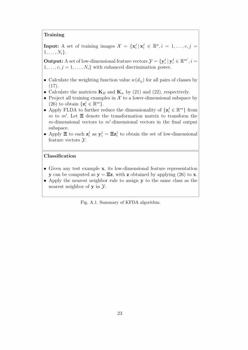
Figure A.1 summarizes the KFDA algorithm for feature extraction which is

11

used with the nearest neighbor rule for classification. In the next section, wepropose a further extension of the KFDA algorithm by introducing two newkernel functions.

3.2 New Kernel Functions

Kernel subspace analysis methods make use of the input data for the compu-tation exclusively in the form of inner products in F , with the inner productscomputed implicitly via a kernel function, called Mercer kernel, k(x,y) =〈φ(x), φ(y)〉, where 〈·, ·〉 is an inner product operator in F . A symmetric func-tion is a Mercer kernel if and only if the Gram matrix formed by applying thisfunction to any finite subset of X is positive semi-definite. Some kernel func-tions such as the polynomial kernel, Gaussian RBF kernel and sigmoid kernelhave been commonly used in many practical applications of kernel methods.For face recognition using kernel subspace analysis methods in particular [6–8,13,17,29,31,32], the polynomial kernel and Gaussian RBF kernel have beenused extensively to demonstrate that kernel subspace analysis methods aremore effective than their linear counterparts in many cases. While in principleany Mercer kernel can be used with kernel subspace analysis methods, not allkernel functions are equally good in terms of the performance that the kernelmethods can deliver.

Recently, the feasibility and effectiveness of different kernel choices for ker-nel subspace analysis methods has been investigated in the context of facerecognition applications. Chen et al. [5] proposed a KDA-based method forface recognition with the parameter of the Gaussian RBF kernel determinedin advance. Yang et al. [26] proposed using a kernel function for KDA bycombining multiple Gaussian RBF kernels with different parameters, with thecombination coefficients determined to optimally combine the individual ker-nels. However, the effectiveness of combining multiple kernels is still implicitfor KDA, since the conventional Fisher criterion in F is converted into thetwo-dimensional Fisher criterion at the same time. Liu et al. [14] extendedthe polynomial kernel to the so-called cosine polynomial kernel by applyingthe cosine measure. One motivation is that the inner product of two vec-tors in F can be regarded as a similarity measure between them. Anothermotivation is that such measure has been found to perform well in practice.Moreover, Liu [11] extended the ordinary polynomial kernel in an innovativeway to include the fractional-power polynomial kernel as well. However, thefractional-power polynomial kernel proposed, like the sigmoid kernel, is nota Mercer kernel. Nevertheless, Liu applied KPCA using the fractional-powerpolynomial kernel for face recognition and showed improvement in perfor-mance when compared with the ordinary polynomial kernel.

12

Inspired by the effectiveness of the cosine measure for kernel functions [14],we further extend the fractional-power polynomial kernel in this paper by in-corporating the cosine measure to give the so-called cosine fractional-powerpolynomial kernel. Note that the cosine measure can only be used with non-stationary kernels such as the polynomial kernel, but not with isotropic kernelssuch as the Gaussian RBF kernel that only depend on the difference betweentwo vectors. To improve the face recognition performance of the GaussianRBF kernel, we also go beyond the traditional Gaussian RBF kernel by con-sidering non-normal Gaussian RBF kernels, kRBF (x,y) = exp(−‖x−y‖d/σ2)where d ≥ 0 and d 6= 2. According to [28], non-normal Gaussian RBF kernelscompletely satisfy the Mercer condition and hence are Mercer kernels if andonly if 0 ≤ d ≤ 2.

In summary, the kernel functions considered in this paper are listed below:

• Polynomial kernel (poly):

kpoly(x,y) = (γ1x · yT − γ2)d with d ∈ N and d ≥ 1. (27)

• Fractional-power polynomial kernel (fp-poly):

kfp−poly(x,y) = (γ1x · yT − γ2)d with 0 < d < 1. (28)

• Cosine polynomial kernel (c-poly):

kc−poly(x,y) =kpoly(x,y)√

kpoly(x,x)kpoly(y,y). (29)

• Cosine fractional-power polynomial kernel (cfp-poly):

kcfp−poly(x,y) =kfp−poly(x,y)√

kfp−poly(x,x)kfp−poly(y,y). (30)

• Gaussian RBF kernel (RBF):

kRBF (x,y) = exp(−‖x− y‖2/σ2). (31)

• Non-normal Gaussian RBF kernel (NN-RBF):

knn−RBF (x,y) = exp(−‖x− y‖d/σ2) with d ≥ 0 and d 6= 2. (32)

13

4 Experimental Results

4.1 Visualization of Data Distributions

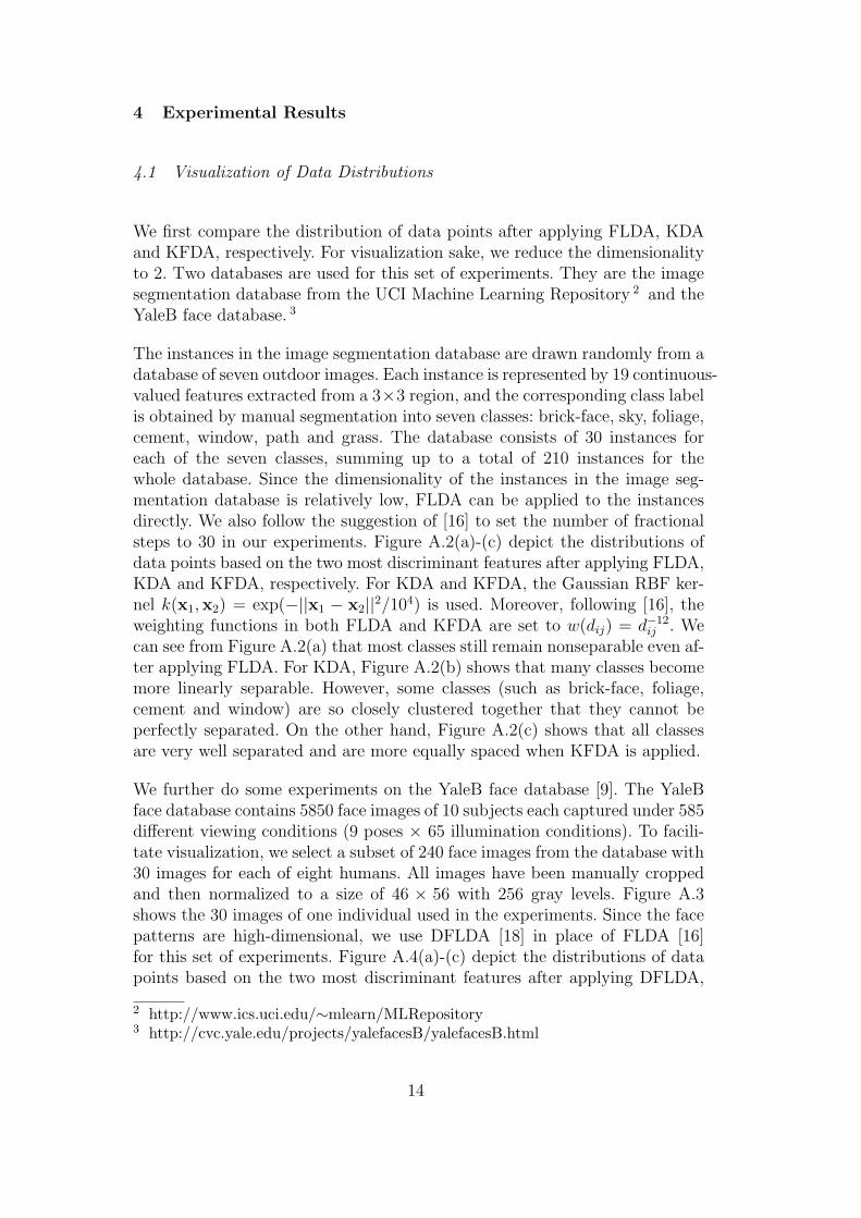
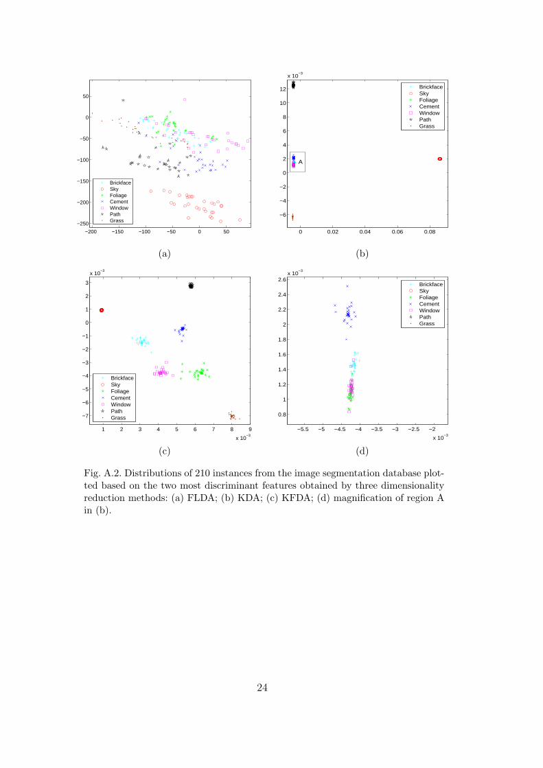
We first compare the distribution of data points after applying FLDA, KDAand KFDA, respectively. For visualization sake, we reduce the dimensionalityto 2. Two databases are used for this set of experiments. They are the imagesegmentation database from the UCI Machine Learning Repository 2 and theYaleB face database. 3

The instances in the image segmentation database are drawn randomly from adatabase of seven outdoor images. Each instance is represented by 19 continuous-valued features extracted from a 3×3 region, and the corresponding class labelis obtained by manual segmentation into seven classes: brick-face, sky, foliage,cement, window, path and grass. The database consists of 30 instances foreach of the seven classes, summing up to a total of 210 instances for thewhole database. Since the dimensionality of the instances in the image seg-mentation database is relatively low, FLDA can be applied to the instancesdirectly. We also follow the suggestion of [16] to set the number of fractionalsteps to 30 in our experiments. Figure A.2(a)-(c) depict the distributions ofdata points based on the two most discriminant features after applying FLDA,KDA and KFDA, respectively. For KDA and KFDA, the Gaussian RBF ker-nel k(x1,x2) = exp(−||x1 − x2||2/104) is used. Moreover, following [16], theweighting functions in both FLDA and KFDA are set to w(dij) = d−12

ij . Wecan see from Figure A.2(a) that most classes still remain nonseparable even af-ter applying FLDA. For KDA, Figure A.2(b) shows that many classes becomemore linearly separable. However, some classes (such as brick-face, foliage,cement and window) are so closely clustered together that they cannot beperfectly separated. On the other hand, Figure A.2(c) shows that all classesare very well separated and are more equally spaced when KFDA is applied.

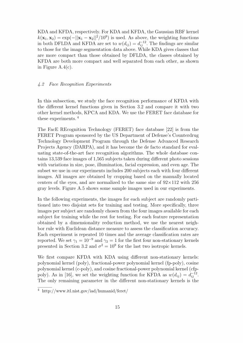
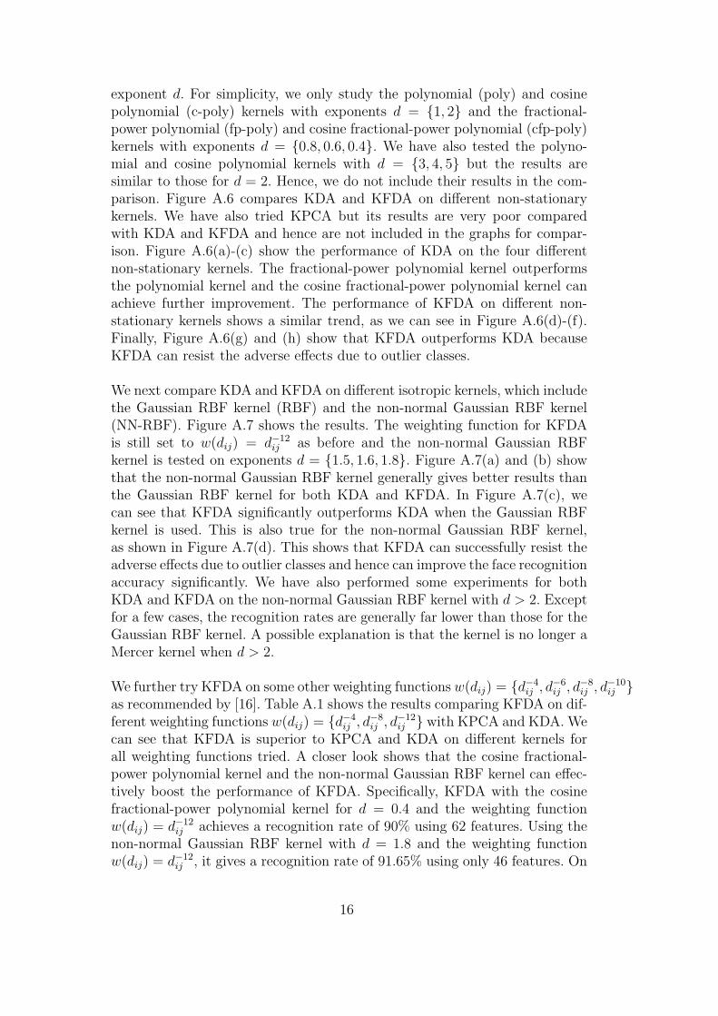
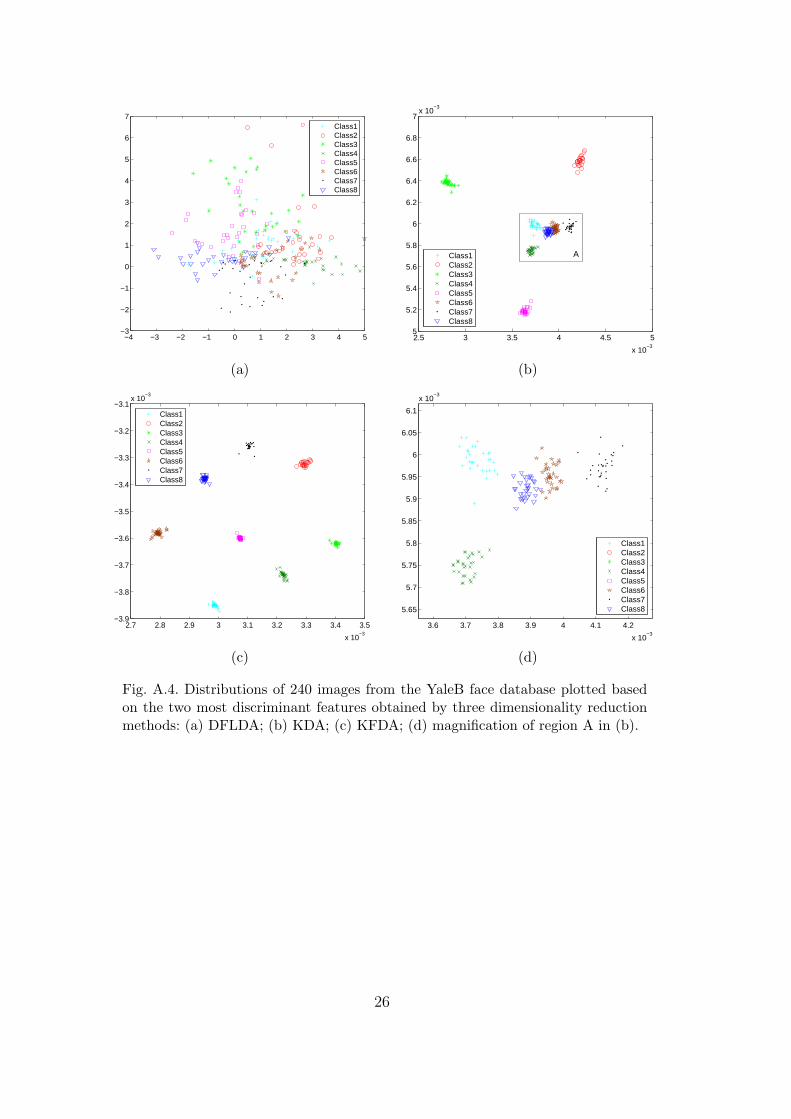
We further do some experiments on the YaleB face database [9]. The YaleBface database contains 5850 face images of 10 subjects each captured under 585different viewing conditions (9 poses × 65 illumination conditions). To facili-tate visualization, we select a subset of 240 face images from the database with30 images for each of eight humans. All images have been manually croppedand then normalized to a size of 46 × 56 with 256 gray levels. Figure A.3shows the 30 images of one individual used in the experiments. Since the facepatterns are high-dimensional, we use DFLDA [18] in place of FLDA [16]for this set of experiments. Figure A.4(a)-(c) depict the distributions of datapoints based on the two most discriminant features after applying DFLDA,

2 http://www.ics.uci.edu/∼mlearn/MLRepository3 http://cvc.yale.edu/projects/yalefacesB/yalefacesB.html

14

KDA and KFDA, respectively. For KDA and KFDA, the Gaussian RBF kernelk(x1,x2) = exp(−||x1 − x2||2/109) is used. As above, the weighting functionsin both DFLDA and KFDA are set to w(dij) = d−12

ij . The findings are similarto those for the image segmentation data above. While KDA gives classes thatare more compact than those obtained by DFLDA, the classes obtained byKFDA are both more compact and well separated from each other, as shownin Figure A.4(c).

4.2 Face Recognition Experiments

In this subsection, we study the face recognition performance of KFDA withthe different kernel functions given in Section 3.2 and compare it with twoother kernel methods, KPCA and KDA. We use the FERET face database forthese experiments. 4

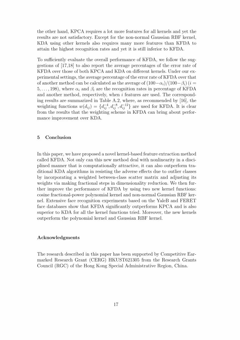
The FacE REcognition Technology (FERET) face database [22] is from theFERET Program sponsored by the US Department of Defense’s CounterdrugTechnology Development Program through the Defense Advanced ResearchProjects Agency (DARPA), and it has become the de facto standard for eval-uating state-of-the-art face recognition algorithms. The whole database con-tains 13,539 face images of 1,565 subjects taken during different photo sessionswith variations in size, pose, illumination, facial expression, and even age. Thesubset we use in our experiments includes 200 subjects each with four differentimages. All images are obtained by cropping based on the manually locatedcenters of the eyes, and are normalized to the same size of 92×112 with 256gray levels. Figure A.5 shows some sample images used in our experiments.

In the following experiments, the images for each subject are randomly parti-tioned into two disjoint sets for training and testing. More specifically, threeimages per subject are randomly chosen from the four images available for eachsubject for training while the rest for testing. For each feature representationobtained by a dimensionality reduction method, we use the nearest neigh-bor rule with Euclidean distance measure to assess the classification accuracy.Each experiment is repeated 10 times and the average classification rates arereported. We set γ1 = 10−9 and γ2 = 1 for the first four non-stationary kernelspresented in Section 3.2 and σ2 = 109 for the last two isotropic kernels.

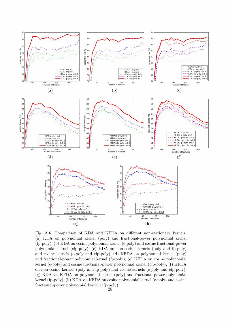
We first compare KFDA with KDA using different non-stationary kernels:polynomial kernel (poly), fractional-power polynomial kernel (fp-poly), cosinepolynomial kernel (c-poly), and cosine fractional-power polynomial kernel (cfp-poly). As in [16], we set the weighting function for KFDA as w(dij) = d−12

ij .The only remaining parameter in the different non-stationary kernels is the

4 http://www.itl.nist.gov/iad/humanid/feret/

15

exponent d. For simplicity, we only study the polynomial (poly) and cosinepolynomial (c-poly) kernels with exponents d = {1, 2} and the fractional-power polynomial (fp-poly) and cosine fractional-power polynomial (cfp-poly)kernels with exponents d = {0.8, 0.6, 0.4}. We have also tested the polyno-mial and cosine polynomial kernels with d = {3, 4, 5} but the results aresimilar to those for d = 2. Hence, we do not include their results in the com-parison. Figure A.6 compares KDA and KFDA on different non-stationarykernels. We have also tried KPCA but its results are very poor comparedwith KDA and KFDA and hence are not included in the graphs for compar-ison. Figure A.6(a)-(c) show the performance of KDA on the four differentnon-stationary kernels. The fractional-power polynomial kernel outperformsthe polynomial kernel and the cosine fractional-power polynomial kernel canachieve further improvement. The performance of KFDA on different non-stationary kernels shows a similar trend, as we can see in Figure A.6(d)-(f).Finally, Figure A.6(g) and (h) show that KFDA outperforms KDA becauseKFDA can resist the adverse effects due to outlier classes.

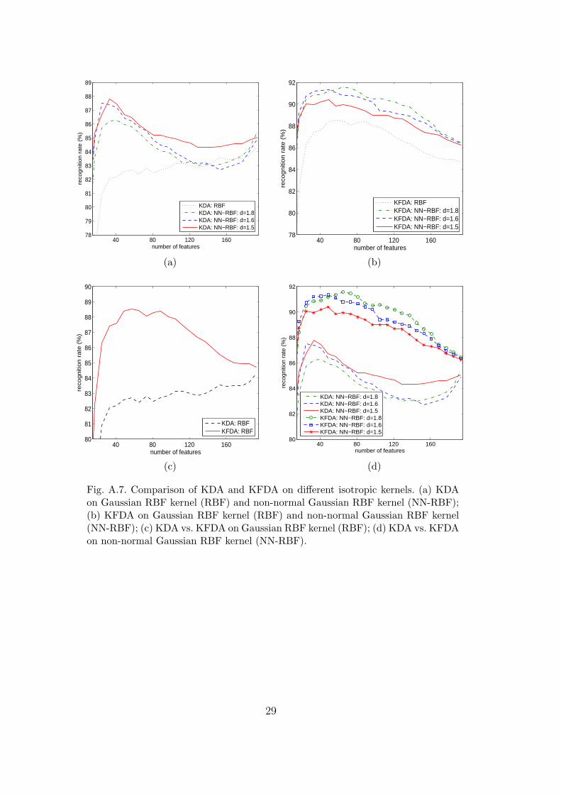
We next compare KDA and KFDA on different isotropic kernels, which includethe Gaussian RBF kernel (RBF) and the non-normal Gaussian RBF kernel(NN-RBF). Figure A.7 shows the results. The weighting function for KFDAis still set to w(dij) = d−12

ij as before and the non-normal Gaussian RBFkernel is tested on exponents d = {1.5, 1.6, 1.8}. Figure A.7(a) and (b) showthat the non-normal Gaussian RBF kernel generally gives better results thanthe Gaussian RBF kernel for both KDA and KFDA. In Figure A.7(c), wecan see that KFDA significantly outperforms KDA when the Gaussian RBFkernel is used. This is also true for the non-normal Gaussian RBF kernel,as shown in Figure A.7(d). This shows that KFDA can successfully resist theadverse effects due to outlier classes and hence can improve the face recognitionaccuracy significantly. We have also performed some experiments for bothKDA and KFDA on the non-normal Gaussian RBF kernel with d > 2. Exceptfor a few cases, the recognition rates are generally far lower than those for theGaussian RBF kernel. A possible explanation is that the kernel is no longer aMercer kernel when d > 2.

We further try KFDA on some other weighting functions w(dij) = {d−4ij , d−6

ij , d−8ij , d−10

ij }as recommended by [16]. Table A.1 shows the results comparing KFDA on dif-ferent weighting functions w(dij) = {d−4

ij , d−8ij , d−12

ij } with KPCA and KDA. Wecan see that KFDA is superior to KPCA and KDA on different kernels forall weighting functions tried. A closer look shows that the cosine fractional-power polynomial kernel and the non-normal Gaussian RBF kernel can effec-tively boost the performance of KFDA. Specifically, KFDA with the cosinefractional-power polynomial kernel for d = 0.4 and the weighting functionw(dij) = d−12

ij achieves a recognition rate of 90% using 62 features. Using thenon-normal Gaussian RBF kernel with d = 1.8 and the weighting functionw(dij) = d−12

ij , it gives a recognition rate of 91.65% using only 46 features. On

16

the other hand, KPCA requires a lot more features for all kernels and yet theresults are not satisfactory. Except for the non-normal Gaussian RBF kernel,KDA using other kernels also requires many more features than KFDA toattain the highest recognition rates and yet it is still inferior to KFDA.

To sufficiently evaluate the overall performance of KFDA, we follow the sug-gestions of [17,18] to also report the average percentages of the error rate ofKFDA over those of both KPCA and KDA on different kernels. Under our ex-perimental settings, the average percentage of the error rate of KFDA over thatof another method can be calculated as the average of (100−αi)/(100−βi) (i =5, . . . , 198), where αi and βi are the recognition rates in percentage of KFDAand another method, respectively, when i features are used. The correspond-ing results are summarized in Table A.2, where, as recommended by [16], theweighting functions w(dij) = {d−4

ij , d−8ij , d−12

ij } are used for KFDA. It is clearfrom the results that the weighting scheme in KFDA can bring about perfor-mance improvement over KDA.

5 Conclusion

In this paper, we have proposed a novel kernel-based feature extraction methodcalled KFDA. Not only can this new method deal with nonlinearity in a disci-plined manner that is computationally attractive, it can also outperform tra-ditional KDA algorithms in resisting the adverse effects due to outlier classesby incorporating a weighted between-class scatter matrix and adjusting itsweights via making fractional steps in dimensionality reduction. We then fur-ther improve the performance of KFDA by using two new kernel functions:cosine fractional-power polynomial kernel and non-normal Gaussian RBF ker-nel. Extensive face recognition experiments based on the YaleB and FERETface databases show that KFDA significantly outperforms KPCA and is alsosuperior to KDA for all the kernel functions tried. Moreover, the new kernelsoutperform the polynomial kernel and Gaussian RBF kernel.

Acknowledgments

The research described in this paper has been supported by Competitive Ear-marked Research Grant (CERG) HKUST621305 from the Research GrantsCouncil (RGC) of the Hong Kong Special Administrative Region, China.

17

References

[1] G. Baudat and F. Anouar. Generalized discriminant analysis using a kernelapproach. Neural Computation, 12:2385–2404, 2000.

[2] P.N. Belhumeur, J.P. Hespanha, and D.J. Kriegman. Eigenfaces vs. Fisherfaces:recognition using class specific linear projection. IEEE Transactions on PatternAnalysis and Machine Intelligence, 19:711–720, July 1997.

[3] H. Cevikalp, M. Neamtu, M. Wilkes, and A. Barkana. Discriminative commonvectors for face recognition. IEEE Transactions on Pattern Analysis andMachine Intelligence, 27(1):4–13, January 2005.

[4] L.F. Chen, H.Y.M. Liao, M.T. Ko, J.C. Lin, and G.J. Yu. A new LDA-basedface recognition system which can solve the small sample size problem. PatternRecognition, 33(10):1713–1726, 2000.

[5] W.S. Chen, P.C. Yuen, J. Huang, and D.Q. Dai. Kernel machine-based one-parameter regularized fisher discriminant method for face recognition. IEEETransactions on System, Man, and Cybernetics-Part B: Cybernetics, 35(4):659–669, August 2005.

[6] G. Dai and Y.T. Qian. Kernel generalized nonlinear discriminant analysisalgorithm for pattern recognition. In Proceedings of the IEEE InternationalConference on Image Processing, pages 2697–2700, 2004.

[7] G. Dai, Y.T. Qian, and S.Jia. A kernel fractional-step nonlinear discriminantanalysis for pattern recognition. In Proceedings of the Eighteenth InternationalConference on Pattern Recognition, volume 2, pages 431–434, August 2004.

[8] G. Dai and D.Y. Yeung. Nonlinear dimensionality reduction for classificationusing kernel weighted subspace method. In Proceedings of the IEEEInternational Conference on Image Processing, pages 838–841, September 2005.

[9] A.S. Georghiades, P.N. Belhumeur, and D.J. Kriegman. From few to many:Illumination cone models for face recognition under variable lighting and pose.IEEE Transactions on Pattern Analysis and Machine Intelligence, 23(6):643–660, 2001.

[10] Y.X. Li, Y.Q. Gao, and H. Erdogan. Weighted pairwise scatter to improvelinear discriminant analysis. In Proceedings of the 6th International Conferenceon Spoken Language Processing, 2000.

[11] C.J. Liu. Gabor-based kernel PCA with fractional power polynomial modelsfor face recognition. IEEE Transactions on Pattern Analysis and MachineIntelligence, 26(5):572–581, May 2004.

[12] C.j. Liu and H. Wechsler. Robust coding schemes for indexing and retrieval fromlarge face databases. IEEE Transactions on Image Processing, 9(1):132–137,January 2000.

18

[13] Q.S. Liu, R. Huang, H.Q. Lu, and S.D. Ma. Face recognition using kernel basedfisher discriminant analysis. In Proceedings of the Fifth IEEE InternationalConference on Automatic Face and Gesture Recognition, pages 187–191, May2002.

[14] Q.S. Liu, H.Q. Lu, and S.D. Ma. Improving kernel Fisher discriminant analysisfor face recognition. IEEE Transactions on Circuits and Systems for VideoTechnology, 14(1):42–49, January 2004.

[15] M. Loog, R.P.W. Duin, and R. Haeb-Umbach. Multiclass linear dimensionreduction by weighted pairwise Fisher criteria. IEEE Transactions on PatternAnalysis and Machine Intelligence, 23(7):762–766, July 2001.

[16] R. Lotlikar and R. Kothari. Fractional-step dimensionality reduction. IEEETransactions on Pattern Analysis and Machine Intelligence, 22(6):623–627,June 2000.

[17] J.W. Lu, K.N. Plataniotis, and A.N. Venetsanopoulos. Face recognition usingkernel direct discriminant analysis algorithms. IEEE Transactions on NeuralNetworks, 14(1):117–126, January 2003.

[18] J.W. Lu, K.N. Plataniotis, and A.N. Venetsanopoulos. Face recognition usingLDA-based algorithms. IEEE Transactions on Neural Networks, 14(1):195–200,January 2003.

[19] J.W. Lu, K.N. Plataniotis, A.N. Venetsanopoulos, and J. Wang. An efficientkernel discriminant analysis method. Pattern Recognition, 38(10):1788–1790,October 2005.

[20] S. Mika, G. Ratsch, J. Weston, B. Scholkopf, and K.R. Muller. Fisherdiscriminant analysis with kernels. In Y.H. Hu, J. Larsen, E. Wilson, andS. Douglas, editors, Proceedings of the Neural Networks for Signal ProcessingIX, pages 41–48, 1999.

[21] B. Moghaddam. Principal manifolds and probabilistic subspaces for visualrecognition. IEEE Transactions on Pattern Analysis and Machine Intelligence,24(6):780–788, June 2002.

[22] A.P.J. Phillips, H.Moon, P.J. Rauss, and S. Rizvi. The FERET evaluationmethodology for face recognition algorithms. IEEE Transactions on PatternAnalysis and Machine Intelligence, 22(10):1090–1104, October 2000.

[23] A.K. Qin, P.N. Suganthan, and M. Loog. Uncorrelated heteroscedastic LDAbased on the weighted pairwise Chernoff criterion. Pattern Recognition,38(4):613–616, 2005.

[24] B. Scholkopf, A. Smola, and K.R. Muller. Nonlinear component analysis as akernel eigenvalue problem. Neural Computation, 10:1299–1319, 1999.

[25] D.L. Swets and J.J. Weng. Using discriminant eigenfeatures for image retrieval.IEEE Transactions on Pattern Analysis and Machine Intelligence, 18(8):831–836, August 1996.

19

[26] S.Yang, S.C Yan, D. Xu, X.O. Tang, and C. Zhang. Fisher+kernel criterion fordiscriminant analysis. In Proceedings of the IEEE Computer Society Conferenceon Computer Vision and Pattern Recognition, pages 197–202, June 2005.

[27] M. Turk and A. Pentland. Eigenfaces for recognition. Journal of CognitiveNeuroscience, 3(1):71–86, 1991.

[28] V. Vapnik. Statistical learning theory. Wiley, New York, 1998.

[29] J. Yang, A.F. Frangi, J.Y. Yang, D. Zhang, and Z. Jin. KPCA plus LDA:a complete kernel Fisher discriminant framework for feature extraction andrecognition. IEEE Transactions on Pattern Analysis and Machine Intelligence,27(2):230–244, February 2005.

[30] J. Yang and J.Y. Yang. Why can LDA be performed in PCA transformedspace? Pattern Recognition, 36(2):563–566, 2003.

[31] M.H. Yang. Kernel eigenfaces vs. kernel Fisherfaces: face recognition usingkernel methods. In Proceedings of the Fifth IEEE International Conference onAutomatic Face and Gesture Recognition, pages 215–220, May 2002.

[32] M.H. Yang, N. Ahuja, and D. Kriegman. Face recognition using kerneleigenfaces. In Proceedings of the IEEE International Conference on ImageProcessing, pages 37–40, 2000.

[33] J. Ye, R. Janardan, C.H. Park, and H. Park. An optimization criterionfor generalized discriminant analysis on undersampled problems. IEEETransactions on Pattern Analysis and Machine Intelligence, 26(8):982–994,August 2004.

[34] J. Ye and Q. Li. A two-stage linear discriminant analysis via QR-decomposition.IEEE Transactions on Pattern Analysis and Machine Intelligence, 27(6):929–941, June 2005.

[35] H. Yu and J. Yang. A direct LDA algorithm for high-dimensional data withapplication to face recognition. Pattern Recognition, 34(11):2067–2070, 2001.

20

A Detailed Derivations

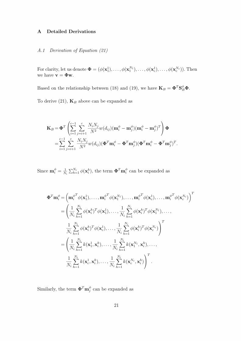
A.1 Derivation of Equation (21)

For clarity, let us denote Φ = (φ(x11), . . . , φ(xN1

1 ), . . . , φ(x1c), . . . , φ(xNc

c )). Thenwe have v = Φw.

Based on the relationship between (18) and (19), we have KB = ΦTSφBΦ.

To derive (21), KB above can be expanded as

KB =ΦT

c−1∑

i=1

c∑

j=i+1

NiNj

N2w(dij)(m

φi −mφ

j )(mφi −mφ

j )T

Φ

=c−1∑

i=1

c∑

j=i+1

NiNj

N2w(dij)(Φ

Tmφi −ΦTmφ

j )(ΦTmφi −ΦTmφ

j )T .

Since mφi = 1

Ni

∑Nih=1 φ(xh

i ), the term ΦTmφi can be expanded as

ΦTmφi =

(mφ

i

Tφ(x1

1), . . . ,mφi

Tφ(xN1

1 ), . . . ,mφi

Tφ(x1

c), . . . ,mφi

Tφ(xNc

c ))T

=

1

Ni

Ni∑

h=1

φ(xhi )

T φ(x11), . . . ,

1

Ni

Ni∑

h=1

φ(xhi )

T φ(xN11 ), . . . ,

1

Ni

Ni∑

h=1

φ(xhi )

T φ(x1c), . . . ,

1

Ni

Ni∑

h=1

φ(xhi )

T φ(xNcc )

T

=

1

Ni

Ni∑

h=1

k(x11,x

hi ), . . . ,

1

Ni

Ni∑

h=1

k(xN11 ,xh

i ), . . . ,

1

Ni

Ni∑

h=1

k(x1c ,x

hi ), . . . ,

1

Ni

Ni∑

h=1

k(xNcc ,xh

i )

T

.

Similarly, the term ΦTmφj can be expanded as

21

ΦTmφj =

1

Nj

Nj∑

h=1

k(x11,x

hj ), . . . ,

1

Nj

Nj∑

h=1

k(xN11 ,xh

j ), . . . ,

1

Nj

Nj∑

h=1

k(x1c ,x

hj ), . . . ,

1

Nj

Nj∑

h=1

k(xNcc ,xh

j )

T

.

For clarity, we denote the expansion of ΦTmφi by mi and the expansion of

ΦTmφj by mj.

Thus,

KB =c−1∑

i=1

c∑

j=i+1

NiNj

N2w(dij)(mi −mj)(mi −mj)

T .

Hence we can obtain equation (21).

A.2 Derivation of Equation (26)

Let Φ = (φ(x11), . . . , φ(xN1

1 ), . . . , φ(x1c), . . . , φ(xNc

c )) and vi = Φwi (i = 1, . . . , m).

Thus, vi = Φwi (i = 1, . . . , m) constitute the discriminant vectors with re-spect to the Fisher criterion J(v) in (18).

Then, the low-dimensional feature representation z = (z1, . . . , zm)T of thevector x can be calculated as

z= (v1, . . . ,vm)T φ(x)

= (w1, . . . ,wm)TΦT φ(x)

= (w1, . . . ,wm)T (φ(x)T φ(x11), . . . , φ(x)T φ(xN1

1 ), . . . , φ(x)T φ(x1c), . . . , φ(x)T φ(xNc

c ))T

= (w1, . . . ,wm)T (k(x11,x), . . . , k(xN1

1 ,x), . . . , k(x1c ,x), . . . , k(xNc

c ,x))T .

Equation (26) can thus be obtained.

22

Training

Input: A set of training images X = {xji |xj

i ∈ Rn, i = 1, . . . , c, j =1, . . . , Ni}.Output: A set of low-dimensional feature vectors Y = {yj

i |yji ∈ Rm′

, i =1, . . . , c, j = 1, . . . , Ni} with enhanced discrimination power.

• Calculate the weighting function value w(dij) for all pairs of classes by(17).

• Calculate the matrices KB and Kw by (21) and (22), respectively.• Project all training examples in X to a lower-dimensional subspace by

(26) to obtain {zji ∈ Rm}.

• Apply FLDA to further reduce the dimensionality of {zji ∈ Rm} from

m to m′. Let Ξ denote the transformation matrix to transform them-dimensional vectors to m′-dimensional vectors in the final outputsubspace.

• Apply Ξ to each zji as yj

i = Ξzji to obtain the set of low-dimensional

feature vectors Y .

Classification

• Given any test example x, its low-dimensional feature representationy can be computed as y = Ξz, with z obtained by applying (26) to x.

• Apply the nearest neighbor rule to assign y to the same class as thenearest neighbor of y in Y .

Fig. A.1. Summary of KFDA algorithm.

23

−200 −150 −100 −50 0 50

−250

−200

−150

−100

−50

0

50

BrickfaceSkyFoliageCementWindowPathGrass

(a)

0 0.02 0.04 0.06 0.08

−6

−4

−2

0

2

4

6

8

10

12

x 10−3

BrickfaceSkyFoliageCementWindowPathGrass

A

(b)

1 2 3 4 5 6 7 8 9

x 10−3

−7

−6

−5

−4

−3

−2

−1

0

1

2

3

x 10−3

BrickfaceSkyFoliageCementWindowPathGrass

(c)

−5.5 −5 −4.5 −4 −3.5 −3 −2.5 −2

x 10−3

0.8

1

1.2

1.4

1.6

1.8

2

2.2

2.4

2.6x 10

−3

BrickfaceSkyFoliageCementWindowPathGrass

(d)

Fig. A.2. Distributions of 210 instances from the image segmentation database plot-ted based on the two most discriminant features obtained by three dimensionalityreduction methods: (a) FLDA; (b) KDA; (c) KFDA; (d) magnification of region Ain (b).

24

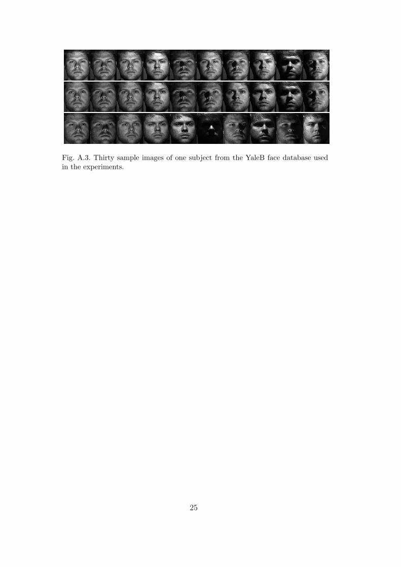
Fig. A.3. Thirty sample images of one subject from the YaleB face database usedin the experiments.

25

−4 −3 −2 −1 0 1 2 3 4 5−3

−2

−1

0

1

2

3

4

5

6

7Class1Class2Class3Class4Class5Class6Class7Class8

(a)

2.5 3 3.5 4 4.5 5

x 10−3

5

5.2

5.4

5.6

5.8

6

6.2

6.4

6.6

6.8

7x 10

−3

Class1Class2Class3Class4Class5Class6Class7Class8

A

(b)

2.7 2.8 2.9 3 3.1 3.2 3.3 3.4 3.5

x 10−3

−3.9

−3.8

−3.7

−3.6

−3.5

−3.4

−3.3

−3.2

−3.1x 10

−3

Class1Class2Class3Class4Class5Class6Class7Class8

(c)

3.6 3.7 3.8 3.9 4 4.1 4.2

x 10−3

5.65

5.7

5.75

5.8

5.85

5.9

5.95

6

6.05

6.1

x 10−3

Class1Class2Class3Class4Class5Class6Class7Class8

(d)

Fig. A.4. Distributions of 240 images from the YaleB face database plotted basedon the two most discriminant features obtained by three dimensionality reductionmethods: (a) DFLDA; (b) KDA; (c) KFDA; (d) magnification of region A in (b).

26

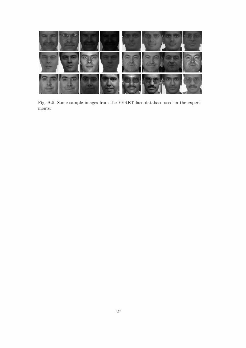
Fig. A.5. Some sample images from the FERET face database used in the experi-ments.

27

40 80 120 16078

79

80

81

82

83

84

85

number of features

reco

gniti

on r

ate

(%)

KDA: poly: d=2KDA: poly: d=1KDA: fp−poly: d=0.8KDA: fp−poly: d=0.6KDA: fp−poly: d=0.4

(a)

40 80 120 16078

79

80

81

82

83

84

85

86

number of featuresre

cogn

ition

rat

e (%

)

KDA: c−poly: d=2KDA: c−poly: d=1KDA: cfp−poly: d=0.8KDA: cfp−poly: d=0.6KDA: cfp−poly: d=0.4

(b)

40 80 120 16078

79

80

81

82

83

84

85

86

number of features

reco

gniti

on r

ate

(%)

KDA: poly: d=2KDA: c−poly: d=2KDA: fp−poly: d=0.6KDA: cfp−poly: d=0.6KDA: fp−poly: d=0.4KDA: cfp−poly: d=0.4

(c)

40 80 120 16080

81

82

83

84

85

86

87

88

89

90

number of features

reco

gniti

on ra

te (%

)

KFDA: ploy: d=2 KFDA: ploy: d=1KFDA: fp−poly: d=0.8 KFDA: fp−poly: d=0.6KFDA: fp−ploy: d=0.4

(d)

40 80 120 16080

81

82

83

84

85

86

87

88

89

90

number of features

reco

gniti

on r

ate

(%)

KFDA: c−poly: d=2KFDA: c−poly: d=1KFDA: cfp−poly: d=0.8KFDA: cfp−poly: d=0.6KFDA: cfp−poly: d=0.4

(e)

40 80 120 16080

81

82

83

84

85

86

87

88

89

90

number of features

reco

gniti

on r

ate

(%)

KFDA: poly: d=2KFDA: c−poly: d=2KFDA: fp−poly: d=0.6KFDA: cfp−poly: d=0.6KFDA: fp−poly: d=0.4KFDA: cfp−poly: d=0.4

(f)

40 80 120 16076

78

80

82

84

86

88

90

number of features

reco

gn

itio

n r

ate

(%

)

KDA: poly: d=2KDA: fp−poly: d=0.4KFDA: poly: d=2KFDA: fp−poly: d=0.4

(g)

40 80 120 16076

78

80

82

84

86

88

90

number of features

reco

gniti

on r

ate

(%)

KDA: c−poly: d=2KDA: cfp−poly: d=0.4KFDA: c−poly: d=2KFDA: cfp−poly: d=0.4

(h)

Fig. A.6. Comparison of KDA and KFDA on different non-stationary kernels.(a) KDA on polynomial kernel (poly) and fractional-power polynomial kernel(fp-poly); (b) KDA on cosine polynomial kernel (c-poly) and cosine fractional-powerpolynomial kernel (cfp-poly); (c) KDA on non-cosine kernels (poly and fp-poly)and cosine kernels (c-poly and cfp-poly); (d) KFDA on polynomial kernel (poly)and fractional-power polynomial kernel (fp-poly); (e) KFDA on cosine polynomialkernel (c-poly) and cosine fractional-power polynomial kernel (cfp-poly); (f) KFDAon non-cosine kernels (poly and fp-poly) and cosine kernels (c-poly and cfp-poly);(g) KDA vs. KFDA on polynomial kernel (poly) and fractional-power polynomialkernel (fp-poly); (h) KDA vs. KFDA on cosine polynomial kernel (c-poly) and cosinefractional-power polynomial kernel (cfp-poly).

28

40 80 120 16078

79

80

81

82

83

84

85

86

87

88

89

number of features

reco

gn

itio

n r

ate

(%

)

KDA: RBFKDA: NN−RBF: d=1.8KDA: NN−RBF: d=1.6KDA: NN−RBF: d=1.5

(a)

40 80 120 16078

80

82

84

86

88

90

92

number of features

reco

gn

itio

n r

ate

(%

)

KFDA: RBFKFDA: NN−RBF: d=1.8KFDA: NN−RBF: d=1.6KFDA: NN−RBF: d=1.5

(b)

40 80 120 16080

81

82

83

84

85

86

87

88

89

90

number of features

reco

gn

itio

n r

ate

(%

)

KDA: RBFKFDA: RBF

(c)

40 80 120 16080

82

84

86

88

90

92

number of features

reco

gniti

on r

ate

(%)

KDA: NN−RBF: d=1.8KDA: NN−RBF: d=1.6KDA: NN−RBF: d=1.5KFDA: NN−RBF: d=1.8KFDA: NN−RBF: d=1.6KFDA: NN−RBF: d=1.5

(d)

Fig. A.7. Comparison of KDA and KFDA on different isotropic kernels. (a) KDAon Gaussian RBF kernel (RBF) and non-normal Gaussian RBF kernel (NN-RBF);(b) KFDA on Gaussian RBF kernel (RBF) and non-normal Gaussian RBF kernel(NN-RBF); (c) KDA vs. KFDA on Gaussian RBF kernel (RBF); (d) KDA vs. KFDAon non-normal Gaussian RBF kernel (NN-RBF).

29

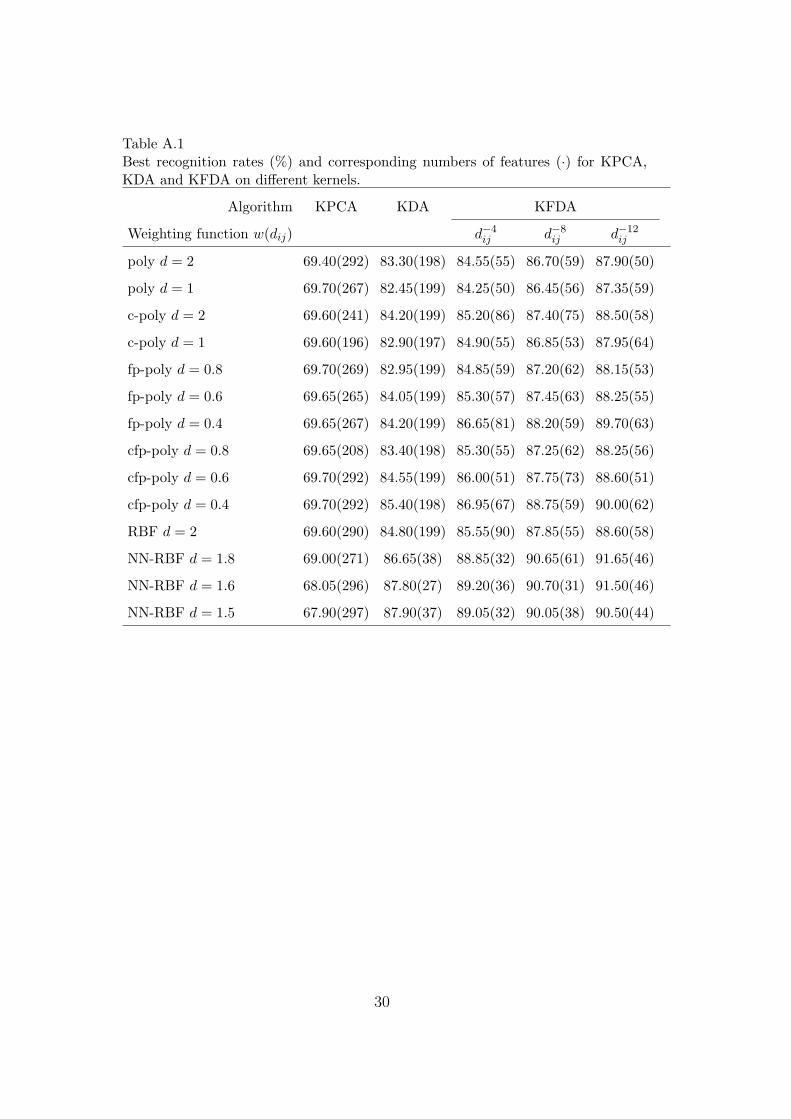
Table A.1Best recognition rates (%) and corresponding numbers of features (·) for KPCA,KDA and KFDA on different kernels.

Algorithm KPCA KDA KFDA

Weighting function w(dij) d−4ij d−8

ij d−12ij

poly d = 2 69.40(292) 83.30(198) 84.55(55) 86.70(59) 87.90(50)

poly d = 1 69.70(267) 82.45(199) 84.25(50) 86.45(56) 87.35(59)

c-poly d = 2 69.60(241) 84.20(199) 85.20(86) 87.40(75) 88.50(58)

c-poly d = 1 69.60(196) 82.90(197) 84.90(55) 86.85(53) 87.95(64)

fp-poly d = 0.8 69.70(269) 82.95(199) 84.85(59) 87.20(62) 88.15(53)

fp-poly d = 0.6 69.65(265) 84.05(199) 85.30(57) 87.45(63) 88.25(55)

fp-poly d = 0.4 69.65(267) 84.20(199) 86.65(81) 88.20(59) 89.70(63)

cfp-poly d = 0.8 69.65(208) 83.40(198) 85.30(55) 87.25(62) 88.25(56)

cfp-poly d = 0.6 69.70(292) 84.55(199) 86.00(51) 87.75(73) 88.60(51)

cfp-poly d = 0.4 69.70(292) 85.40(198) 86.95(67) 88.75(59) 90.00(62)

RBF d = 2 69.60(290) 84.80(199) 85.55(90) 87.85(55) 88.60(58)

NN-RBF d = 1.8 69.00(271) 86.65(38) 88.85(32) 90.65(61) 91.65(46)

NN-RBF d = 1.6 68.05(296) 87.80(27) 89.20(36) 90.70(31) 91.50(46)

NN-RBF d = 1.5 67.90(297) 87.90(37) 89.05(32) 90.05(38) 90.50(44)

30

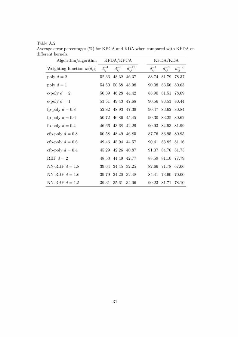
Table A.2Average error percentages (%) for KPCA and KDA when compared with KFDA ondifferent kernels.

Algorithm/algorithm KFDA/KPCA KFDA/KDA

Weighting function w(dij) d−4ij d−8

ij d−12ij d−4

ij d−8ij d−12

ij

poly d = 2 52.36 48.32 46.37 88.74 81.79 78.37

poly d = 1 54.50 50.58 48.98 90.08 83.56 80.63

c-poly d = 2 50.39 46.28 44.42 88.90 81.51 78.09

c-poly d = 1 53.51 49.43 47.68 90.56 83.53 80.44

fp-poly d = 0.8 52.82 48.93 47.39 90.47 83.62 80.84

fp-poly d = 0.6 50.72 46.86 45.45 90.30 83.25 80.62

fp-poly d = 0.4 46.66 43.68 42.29 90.93 84.93 81.99

cfp-poly d = 0.8 50.58 48.49 46.85 87.76 83.95 80.95

cfp-poly d = 0.6 49.46 45.94 44.57 90.41 83.82 81.16

cfp-poly d = 0.4 45.29 42.26 40.87 91.07 84.76 81.75

RBF d = 2 48.53 44.49 42.77 88.59 81.10 77.79

NN-RBF d = 1.8 39.64 34.45 32.25 82.66 71.78 67.06

NN-RBF d = 1.6 39.79 34.20 32.48 84.41 73.90 70.00

NN-RBF d = 1.5 39.31 35.61 34.06 90.23 81.71 78.10

31

About the Author − GUANG DAI received his B.Eng. degree in Mechan-ical Engineering from Dalian University of Technology and M.Phil. degree inComputer Science from Zhejiang University. He is currently a PhD studentin the Department of Computer Science and Engineering at the Hong KongUniversity of Science and Technology. His main research interests include semi-supervised learning, nonlinear dimensionality reduction, and related applica-tions.

About the Author − DIT-YAN YEUNG received his B.Eng. degree inElectrical Engineering and M.Phil. degree in Computer Science from the Uni-versity of Hong Kong, and his Ph.D. degree in Computer Science from theUniversity of Southern California in Los Angeles. He was an Assistant Pro-fessor at the Illinois Institute of Technology in Chicago before he joined theDepartment of Computer Science and Engineering at the Hong Kong Univer-sity of Science and Technology, where he is currently an Associate Professor.His current research interests are in machine learning and pattern recognition.

About the Author − YUN-TAO QIAN received his B.E. and M.E. degreesin automatic control from Xi’an Jiaotong University in 1989 and 1992, respec-tively, and his Ph.D. degree in signal processing from Xidian University in1996. From 1996 to 1998, he was a postdoctoral fellow at the NorthwesternPolytechnical University. Since 1998, he has been with Zhejiang Universitywhere he is currently a Professor in Computer Science. His research interestsinclude machine learning, signal and image processing, and pattern recogni-tion.

32