Face Recognition

Wei-Lun Chao

GICE, National Taiwan University

Abstract

Face recognition has been one of the most interesting and important research fields

in the past two decades. The reasons come from the need of automatic recognitions

and surveillance systems, the interest in human visual system on face recognition,

and the design of human-computer interface, etc. These researches involve know-

ledge and researchers from disciplines such as neuroscience, psychology, computer

vision, pattern recognition, image processing, and machine learning, etc. A bunch of

papers have been published to overcome difference factors (such as illumination, ex-

pression, scale, pose, ……) and achieve better recognition rate, while there is still no

robust technique against uncontrolled practical cases which may involve kinds of

factors simultaneously. In this report, we’ll go through general ideas and structures

of recognition, important issues and factors of human faces, critical techniques and

algorithms, and finally give a comparison and conclusion. Readers who are interested

in face recognition could also refer to published surveys [1-3] and website about face

recognition [4]. To be announced, this report only focuses on color-image-based (2D)

face recognition, rather than video-based (3D) and thermal-image-based methods.

Table of content:

(1) Introduction to face recognition: Structure and Procedure

(2) Fundamental of pattern recognition

(3) Issues and factors of human faces

(4) Techniques and algorithms on face detection

(5) Techniques and algorithms on face feature extraction and face recognition

(6) Comparison and Conclusion

1. Introduction to Face Recognition: Structure and Procedure

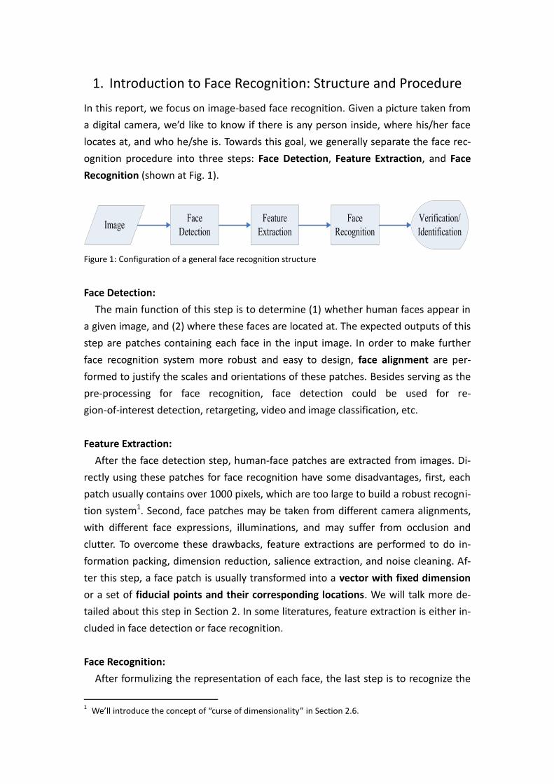
In this report, we focus on image-based face recognition. Given a picture taken from

a digital camera, we’d like to know if there is any person inside, where his/her face

locates at, and who he/she is. Towards this goal, we generally separate the face rec-

ognition procedure into three steps: Face Detection, Feature Extraction, and Face

Recognition (shown at Fig. 1).

Face

Detection

Feature

Extraction

Face

RecognitionImage

Verification/

Identification

Figure 1: Configuration of a general face recognition structure

Face Detection:

The main function of this step is to determine (1) whether human faces appear in

a given image, and (2) where these faces are located at. The expected outputs of this

step are patches containing each face in the input image. In order to make further

face recognition system more robust and easy to design, face alignment are per-

formed to justify the scales and orientations of these patches. Besides serving as the

pre-processing for face recognition, face detection could be used for re-

gion-of-interest detection, retargeting, video and image classification, etc.

Feature Extraction:

After the face detection step, human-face patches are extracted from images. Di-

rectly using these patches for face recognition have some disadvantages, first, each

patch usually contains over 1000 pixels, which are too large to build a robust recogni-

tion system1. Second, face patches may be taken from different camera alignments,

with different face expressions, illuminations, and may suffer from occlusion and

clutter. To overcome these drawbacks, feature extractions are performed to do in-

formation packing, dimension reduction, salience extraction, and noise cleaning. Af-

ter this step, a face patch is usually transformed into a vector with fixed dimension

or a set of fiducial points and their corresponding locations. We will talk more de-

tailed about this step in Section 2. In some literatures, feature extraction is either in-

cluded in face detection or face recognition.

Face Recognition:

After formulizing the representation of each face, the last step is to recognize the

1 We’ll introduce the concept of “curse of dimensionality” in Section 2.6.

identities of these faces. In order to achieve automatic recognition, a face database is

required to build. For each person, several images are taken and their features are

extracted and stored in the database. Then when an input face image comes in, we

perform face detection and feature extraction, and compare its feature to each face

class stored in the database. There have been many researches and algorithms pro-

posed to deal with this classification problem, and we’ll discuss them in later sections.

There are two general applications of face recognition, one is called identification

and another one is called verification. Face identification means given a face image,

we want the system to tell who he / she is or the most probable identification; while

in face verification, given a face image and a guess of the identification, we want the

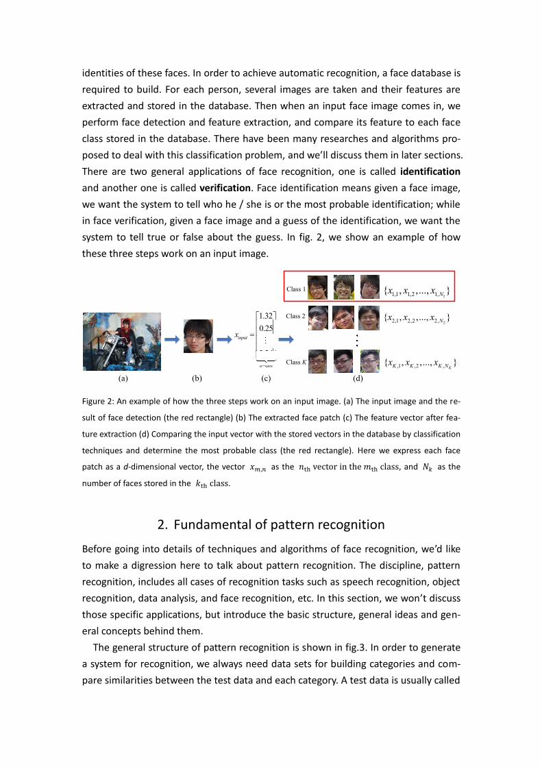
system to tell true or false about the guess. In fig. 2, we show an example of how

these three steps work on an input image.

dim

1.32

0.25

3.24

input

d

x

Class 1

Class 2

Class K

22,1 2,2 2,{ , ,..., }Nx x x

11,1 1,2 1,{ , ,..., }Nx x x

,1 ,2 ,{ , ,..., }KK K K Nx x x

(a) (b) (c) (d)

Figure 2: An example of how the three steps work on an input image. (a) The input image and the re-

sult of face detection (the red rectangle) (b) The extracted face patch (c) The feature vector after fea-

ture extraction (d) Comparing the input vector with the stored vectors in the database by classification

techniques and determine the most probable class (the red rectangle). Here we express each face

patch as a d-dimensional vector, the vector as the , and as the

number of faces stored in the .

2. Fundamental of pattern recognition

Before going into details of techniques and algorithms of face recognition, we’d like

to make a digression here to talk about pattern recognition. The discipline, pattern

recognition, includes all cases of recognition tasks such as speech recognition, object

recognition, data analysis, and face recognition, etc. In this section, we won’t discuss

those specific applications, but introduce the basic structure, general ideas and gen-

eral concepts behind them.

The general structure of pattern recognition is shown in fig.3. In order to generate

a system for recognition, we always need data sets for building categories and com-

pare similarities between the test data and each category. A test data is usually called

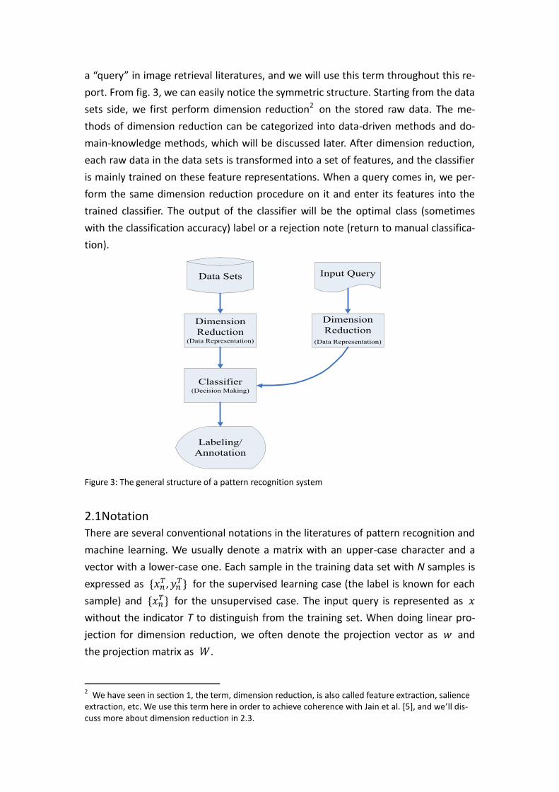
a “query” in image retrieval literatures, and we will use this term throughout this re-

port. From fig. 3, we can easily notice the symmetric structure. Starting from the data

sets side, we first perform dimension reduction2 on the stored raw data. The me-

thods of dimension reduction can be categorized into data-driven methods and do-

main-knowledge methods, which will be discussed later. After dimension reduction,

each raw data in the data sets is transformed into a set of features, and the classifier

is mainly trained on these feature representations. When a query comes in, we per-

form the same dimension reduction procedure on it and enter its features into the

trained classifier. The output of the classifier will be the optimal class (sometimes

with the classification accuracy) label or a rejection note (return to manual classifica-

tion).

Dimension

Reduction(Data Representation)

Dimension

Reduction

(Data Representation)

Classifier(Decision Making)

Data Sets Input Query

Labeling/

Annotation

Figure 3: The general structure of a pattern recognition system

2.1 Notation There are several conventional notations in the literatures of pattern recognition and

machine learning. We usually denote a matrix with an upper-case character and a

vector with a lower-case one. Each sample in the training data set with N samples is

expressed as

for the supervised learning case (the label is known for each

sample) and for the unsupervised case. The input query is represented as

without the indicator T to distinguish from the training set. When doing linear pro-

jection for dimension reduction, we often denote the projection vector as and

the projection matrix as .

2 We have seen in section 1, the term, dimension reduction, is also called feature extraction, salience

extraction, etc. We use this term here in order to achieve coherence with Jain et al. [5], and we’ll dis-cuss more about dimension reduction in 2.3.

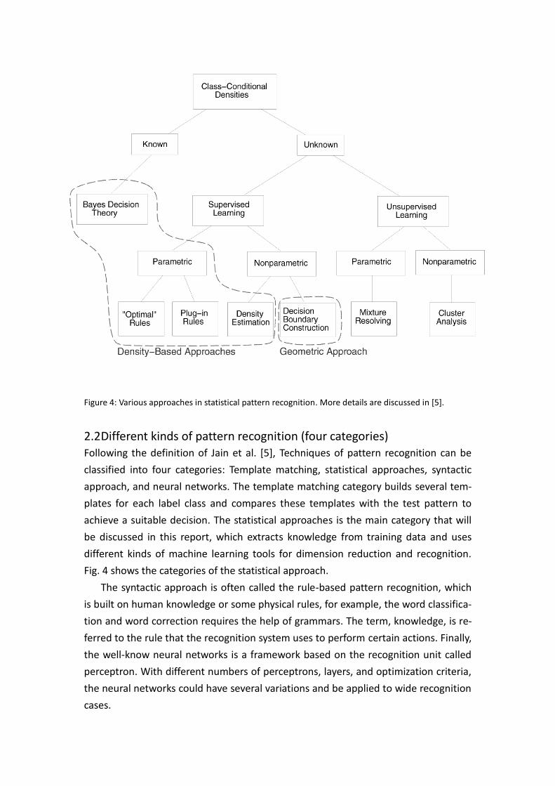
Figure 4: Various approaches in statistical pattern recognition. More details are discussed in [5].

2.2 Different kinds of pattern recognition (four categories) Following the definition of Jain et al. [5], Techniques of pattern recognition can be

classified into four categories: Template matching, statistical approaches, syntactic

approach, and neural networks. The template matching category builds several tem-

plates for each label class and compares these templates with the test pattern to

achieve a suitable decision. The statistical approaches is the main category that will

be discussed in this report, which extracts knowledge from training data and uses

different kinds of machine learning tools for dimension reduction and recognition.

Fig. 4 shows the categories of the statistical approach.

The syntactic approach is often called the rule-based pattern recognition, which

is built on human knowledge or some physical rules, for example, the word classifica-

tion and word correction requires the help of grammars. The term, knowledge, is re-

ferred to the rule that the recognition system uses to perform certain actions. Finally,

the well-know neural networks is a framework based on the recognition unit called

perceptron. With different numbers of perceptrons, layers, and optimization criteria,

the neural networks could have several variations and be applied to wide recognition

cases.

2.3 Dimension Reduction: Domain-knowledge Approach and Data-driven

Approach Dimension reduction is one of the most important steps in pattern recognition and

machine learning. It’s difficult to directly use the raw data (ex. face patches) for pat-

tern recognition not only because significant parts of the data haven’t been extracted

but also because the extremely high dimensionality of the raw data. Significant parts

(for recognition purposes or the parts with more interest) usually occupy just a small

portion of the raw data and cannot directly be extracted by simple methods such as

cropping and sampling. For example, a one-channel audio signal usually contains

over 10000 samples per second, and there will be over 1800000 samples for a three

minute-long song. Directly using the raw signal for music genre recognition is prohi-

bitive and we may seek to extract useful music features such as pitch, tempo, and

information of instruments which could better express our auditory perception. The

goal of dimension reduction is to extract useful information and reduce the dimen-

sionality of input data into classifiers in order to decrease the cost of computation

and solve the curse of dimensionality problem.

There’re two main categories of dimension reduction techniques: domain-

knowledge approaches and data-driven approaches. The domain-knowledge ap-

proaches perform dimension reduction based on knowledge of the specific pattern

recognition case. For example, in image processing and audio signal processing, the

discrete Fourier transform (DFT) discrete cosine transform (DCT) and discrete wavelet

transform are frequently used because of the nature that human visual and auditory

perception have higher response at low frequencies than high frequencies. Another

significant example is the use of language model in text retrieval which includes the

contextual environment of languages.

In contrast to the domain-knowledge approaches, the data-driven approaches

directly extract useful features from the training data by some kinds of machine

learning techniques. For example, the eigenface which will be discussed in Section

5.11 determines the most important projection bases based on the principal com-

ponent analysis which are dependent on the training data set, not the fixed basis like

the DFT or DCT. In section 5, we’ll see more examples about these two dimension

reduction categories.

2.4 Two tasks: Unsupervised Learning and Supervised Learning There’re two general tasks in pattern recognition and machine learning: supervised

learning and unsupervised learning. The main difference between these two tasks is

if the label of each training sample is known or unknown. When the label is known,

then during the learning phase in pattern recognition, we’re trying to model the rela-

tion between the feature vectors and their corresponding labels, and this kind of

learning is called the supervised learning. On the other hand, if the label of each

training sample is unknown, then what we try to learn is the distribution of the

possible categories of feature vectors in the training data set, and this kind of learn-

ing is called the unsupervised learning. In fact, there is another task of learning called

the semi-supervised learning, which means only part of the training data has labels,

while this kind of learning is beyond the scope of this report.

2.5 Evaluation Methods Besides the choices of pattern recognition methods, we also need to evaluate the

performance of the experiments. There are two main evaluation plots: the ROC (re-

ceiver operating characteristics) curve and the PR (precision and recall) curve. The

ROC curve examines the relation between the true positive rate and the false posi-

tive rate, while the PR curve extracts the relation between detection rate (recall) and

the detection precision. In the two-class recognition case (for example, face and

non-face), the true positive means the portion of face images to be detected by the

system, while the false positive means the portion of non-face images to de detected

as faces. The term true positive here has the same meaning as the detection rate and

recall and we give a detailed description in table 1 and table 2. In fig. 5, we show

examples of the PR curve. In addition to using curves for evaluation, there’re some

frequently used values for performance judgments, and we summarize them in table

3.

The threshold used to decide the positive or negative for a given case plays an

important role in pattern recognition. With low threshold, we could achieve high true

positive rate but also high false positive rate, and vice versa. To be noticed, each

point on the ROC curve or PR curve corresponds to a specific threshold used.

The terms positive and negative reveal the asymmetric condition on detection

tasks where one class is the desired pattern class and another class is the comple-

ment class. While in tasks that each class has equal importance or similar meaning

(for example, each class denotes one kind of object), the error rate is much pre-

ferred.

Table 1: The definition of true positive and false positive

Ground truth \ detection Detected (positive) Rejected (negative)

Desired class True positive (TP) False negative (FN)

Complement class False positive (FP) True negative (TN)

(The ground truth means the given labels of the validation samples)

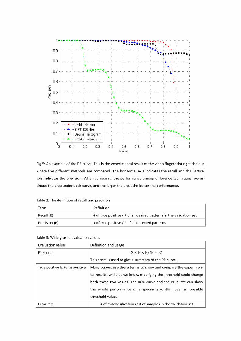
Fig 5: An example of the PR curve. This is the experimental result of the video fingerprinting technique,

where five different methods are compared. The horizontal axis indicates the recall and the vertical

axis indicates the precision. When comparing the performance among difference techniques, we es-

timate the area under each curve, and the larger the area, the better the performance.

Table 2: The definition of recall and precision

Term Definition

Recall (R) # of true positive / # of all desired patterns in the validation set

Precision (P) # of true positive / # of all detected patterns

Table 3: Widely-used evaluation values

Evaluation value Definition and usage

F1 score

This score is used to give a summary of the PR curve.

True positive & False positive Many papers use these terms to show and compare the experimen-

tal results, while as we know, modifying the threshold could change

both these two values. The ROC curve and the PR curve can show

the whole performance of a specific algorithm over all possible

threshold values

Error rate # of misclassifications / # of samples in the validation set

Table 4: The definition of the four vectors in the statistical pattern recognition

Factor Definition

N The size of training data set. In the statistical pattern recognition, the knowledge of di-

mension reduction and classification is extracted from the training set, so the choices and

the number of samples in the training set play important roles in building a robust recog-

nition system. There have been many researches focusing on how to deal with limited

training data size and how to increase the data size by some artificial methods.

d The dimensionality of the feature vectors. In general, more dimensions included will re-

sult in better performance.

C The number of classes. This term determines the scope of the recognition task. For ex-

ample, face detection task could be seen as a two-class recognition task, while face rec-

ognition is a multi-class task.

h The complexity of the classifier. There is no apparent formula to evaluate the complexity

and the most popular judgment is the number of parameters of the adopted classifier.

Table 5: The task to be considered in the statistical pattern recognition and their relationship

Over-fitting/

under-fitting

When training a classifier, we can expect that adopting higher complexity h will

achieve lower error rate on the training set. While for unseen data (data that will

appear for classification later), this classifier may has poor performance because

we don’t have sufficient large training data size N to include all cases of data. On

the other hand, if we adopt lower-complexity classifiers, the performance for

training data and unseen data will both be poor.

To train a higher-complexity classifier, we need a larger training data size to

capture the reliable statistical properties. For a certain training data size, there is a

suitable complexity h to be chosen, which can be estimate by the cross validation

method.

In the statistical pattern recognition category, what we are seeking is the gene-

ralization performance (the performance for unseen data), rather than the per-

formance on the training data. If we adopt a higher complexity than a suitable

one, we’ll get a lower training error but higher generalized error, this condition is

called “over-fitting”. In contrast, if a lower complexity is sued, we’ll achieve both

higher error rates on these two cases, and this condition is called “under-fitting”.

The curse of

dimensionality

With higher dimensionality d, we need large training data size N to capture the

approximate distribution of the desired classes. While in many cases, data acquisi-

tion is fairly difficult and only a small data size is available, then we may suffer

from the curse of dimensionality problem which results in poor statistical estima-

tion and inference. To solve this problem, we need to perform dimension reduc-

tion.

2.6 Conclusion The tasks and cases discussed in the previous sections give an overview about pat-

tern recognition. To gain more insight on the performance of pattern recognition

techniques, we need to take care about some important factors. In template match-

ing, the number of templates for each class and the adopted distance metric directly

affects the recognition result. In statistical pattern recognition, there are four impor-

tant factors: the size of the training data N, the dimensionality of each feature vec-

tor d, the number of classes C, and the complexity of the classifier h, and we sum-

marize their meanings and relations in table 4 and table 5. In syntactic approach, we

expect that the more rules are considered, the higher recognition performance we

can achieve, while the system will become more complicated. And sometimes, it’s

hard to transfer and organize human knowledge into algorithms. Finally in neural

networks, the number of layers, the number of used perceptrons (neurons), the di-

mensionality of feature vectors, and the number of classes all have effects on the

recognition performance. More interesting, the neural networks have been discussed

and proved to have closed relationships with the statistical pattern recognition tech-

niques [5].

3. Issues and factors of human faces

In section 2, we have introduced the general picture of pattern recognition, and from

this section on, we’ll go into one of its applications, face recognition. When focusing

on a specific application, besides building the general structure of pattern recogni-

tion system, we also need to consider the intrinsic properties of the domain-specific

data. For example, to analyze music or speech, we may first transform the input sig-

nal into frequency domain or MFCC (Mel-frequency cepstral coefficients) because

features represented in these domain have been proved to better capture human

auditory perception. In this section, we’ll talk about the domain-knowledge of hu-

man faces, factors that result in face-appearance variations in images, and finally list

important issues to be considered when designing a face recognition system.

3.1 Domain-knowledge of human faces and human visual system

3.1.1 Aspects from psychophysics and neuroscience

There are several researches in psychophysics and neuroscience studying about how

we human performs recognition processes, and many of them have direct relevance

to engineers interested in designing algorithms or systems for machine recognition

of faces. In this subsection, we briefly review several interesting aspects. The first

argument in these disciplines is that whether face recognition a dedicated process

against other object recognition tasks. Evidences that (1) faces are more easily re-

membered by humans than other objects when presented in an upright orientation

and (2) prosopagnosia patients can recognize faces from other objects but have dif-

ficulty in identifying the face support the viewpoint of face recognition as a dedicat-

ed process. While recently, some findings in human neuropsychology and neuroi-

maging suggest that face recognition may not be unique [2].

3.1.2 Holistic-based or feature-based

This is another interesting argument in psychophysics / neuroscience as well as in

algorithm design. The holistic-based viewpoint claims that human recognize faces by

the global appearances, while the feature-based viewpoint believes that important

features such as eyes, noses, and mouths play dominant roles in identifying and re-

membering a person. The design of face recognition algorithms also apply these

perspectives and will be discussed in Section 5.

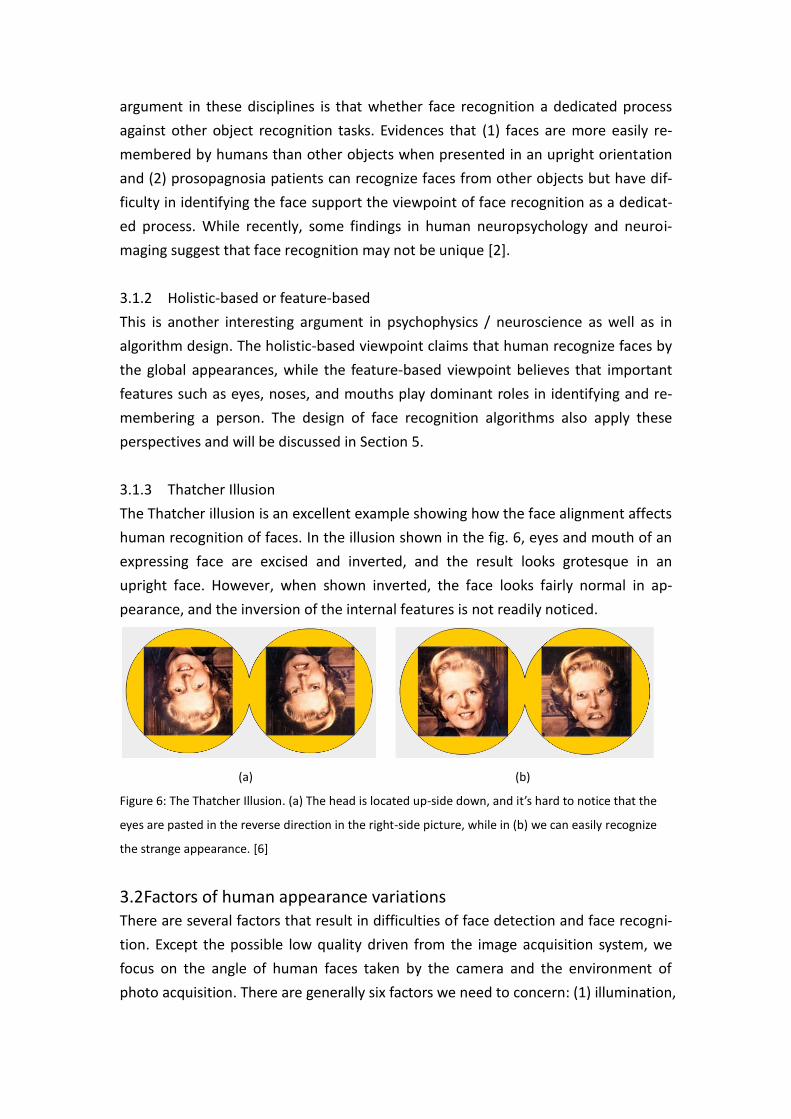
3.1.3 Thatcher Illusion

The Thatcher illusion is an excellent example showing how the face alignment affects

human recognition of faces. In the illusion shown in the fig. 6, eyes and mouth of an

expressing face are excised and inverted, and the result looks grotesque in an

upright face. However, when shown inverted, the face looks fairly normal in ap-

pearance, and the inversion of the internal features is not readily noticed.

(a) (b)

Figure 6: The Thatcher Illusion. (a) The head is located up-side down, and it’s hard to notice that the

eyes are pasted in the reverse direction in the right-side picture, while in (b) we can easily recognize

the strange appearance. [6]

3.2 Factors of human appearance variations There are several factors that result in difficulties of face detection and face recogni-

tion. Except the possible low quality driven from the image acquisition system, we

focus on the angle of human faces taken by the camera and the environment of

photo acquisition. There are generally six factors we need to concern: (1) illumination,

(2) face pose, (3) face expression, (4) RST (rotation, scale, and translation) variation,

(5) clutter background, and (6) occlusion. Table 6 lists the details of each factor.

Table 6: The list and description of the six general factors

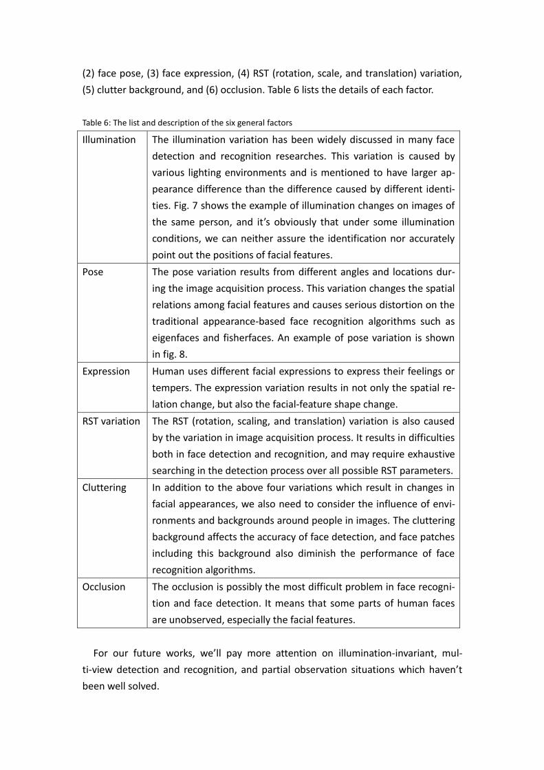
Illumination The illumination variation has been widely discussed in many face

detection and recognition researches. This variation is caused by

various lighting environments and is mentioned to have larger ap-

pearance difference than the difference caused by different identi-

ties. Fig. 7 shows the example of illumination changes on images of

the same person, and it’s obviously that under some illumination

conditions, we can neither assure the identification nor accurately

point out the positions of facial features.

Pose The pose variation results from different angles and locations dur-

ing the image acquisition process. This variation changes the spatial

relations among facial features and causes serious distortion on the

traditional appearance-based face recognition algorithms such as

eigenfaces and fisherfaces. An example of pose variation is shown

in fig. 8.

Expression Human uses different facial expressions to express their feelings or

tempers. The expression variation results in not only the spatial re-

lation change, but also the facial-feature shape change.

RST variation The RST (rotation, scaling, and translation) variation is also caused

by the variation in image acquisition process. It results in difficulties

both in face detection and recognition, and may require exhaustive

searching in the detection process over all possible RST parameters.

Cluttering In addition to the above four variations which result in changes in

facial appearances, we also need to consider the influence of envi-

ronments and backgrounds around people in images. The cluttering

background affects the accuracy of face detection, and face patches

including this background also diminish the performance of face

recognition algorithms.

Occlusion The occlusion is possibly the most difficult problem in face recogni-

tion and face detection. It means that some parts of human faces

are unobserved, especially the facial features.

For our future works, we’ll pay more attention on illumination-invariant, mul-

ti-view detection and recognition, and partial observation situations which haven’t

been well solved.

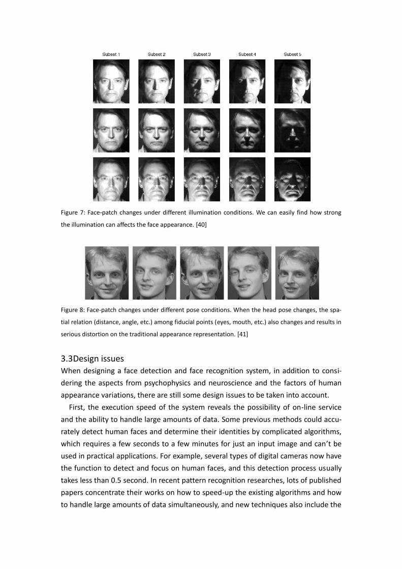
Figure 7: Face-patch changes under different illumination conditions. We can easily find how strong

the illumination can affects the face appearance. [40]

Figure 8: Face-patch changes under different pose conditions. When the head pose changes, the spa-

tial relation (distance, angle, etc.) among fiducial points (eyes, mouth, etc.) also changes and results in

serious distortion on the traditional appearance representation. [41]

3.3 Design issues When designing a face detection and face recognition system, in addition to consi-

dering the aspects from psychophysics and neuroscience and the factors of human

appearance variations, there are still some design issues to be taken into account.

First, the execution speed of the system reveals the possibility of on-line service

and the ability to handle large amounts of data. Some previous methods could accu-

rately detect human faces and determine their identities by complicated algorithms,

which requires a few seconds to a few minutes for just an input image and can’t be

used in practical applications. For example, several types of digital cameras now have

the function to detect and focus on human faces, and this detection process usually

takes less than 0.5 second. In recent pattern recognition researches, lots of published

papers concentrate their works on how to speed-up the existing algorithms and how

to handle large amounts of data simultaneously, and new techniques also include the

execution time in the experimental results as comparison and judgment against oth-

er techniques.

Second, the training data size is another important issue in algorithm design. It is

trivial that more data are included, more information we can exploit and better per-

formance we can achieve. While in practical cases, the database size is usually limited

due to the difficulty in data acquisition and the human privacy. Under the condition

of limited data size, the designed algorithm should not only capture information from

training data but also include some prior knowledge or try to predict and interpolate

the missing and unseen data. In the comparison between the eigenface and the fi-

sherface, it has been examined that under limited data size, the eigenface has better

performance than the fisherface.

Finally, how to bring the algorithms into uncontrolled conditions is yet an unsolved

problem. In Section 3.2, we have mentioned six types of appearance-variant factors,

in our knowledge until now, there is still no technique simultaneously handling these

factors well. For future researches, besides designing new algorithms, we’ll try to

combine the existing algorithms and modify the weights and relationship among

them to see if face detection and recognition could be extended into uncontrolled

conditions.

4. Face detection

From this section on, we start to talk about technical and algorithm aspects of face

recognition. We follow the three-step procedure depicted in fig. 1 and introduce

each step in the order: Face detection is introduced in this section, and feature ex-

traction and face recognition are introduced in the next section. In the survey written

by Yang et al. [7], face detection algorithms are classified into four categories: know-

ledge-based, feature invariant, template matching, and the appearance-based me-

thod. We follow their idea and describe each category and present excellent exam-

ples in the following subsections. To be noticed, there are generally two face detec-

tion cases, one is based on gray level images, and the other one is based on colored

images.

4.1 Knowledge-based methods These rule-based methods encode human knowledge of what constitutes a typi-

cal face. Usually, the rules capture the relationships between facial features. These

methods are designed mainly for face localization, which aims to determine the im-

age position of a single face. In this subsection, we introduce two examples based on

hierarchical knowledge-based method and vertical / horizontal projection.

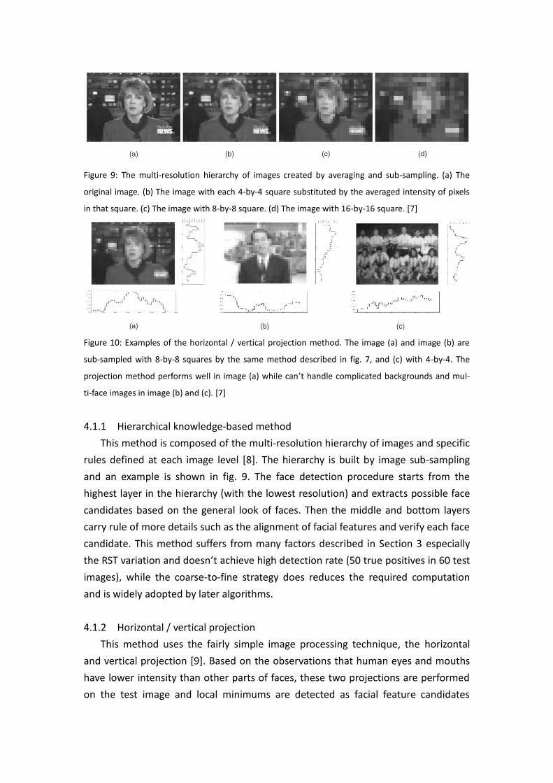
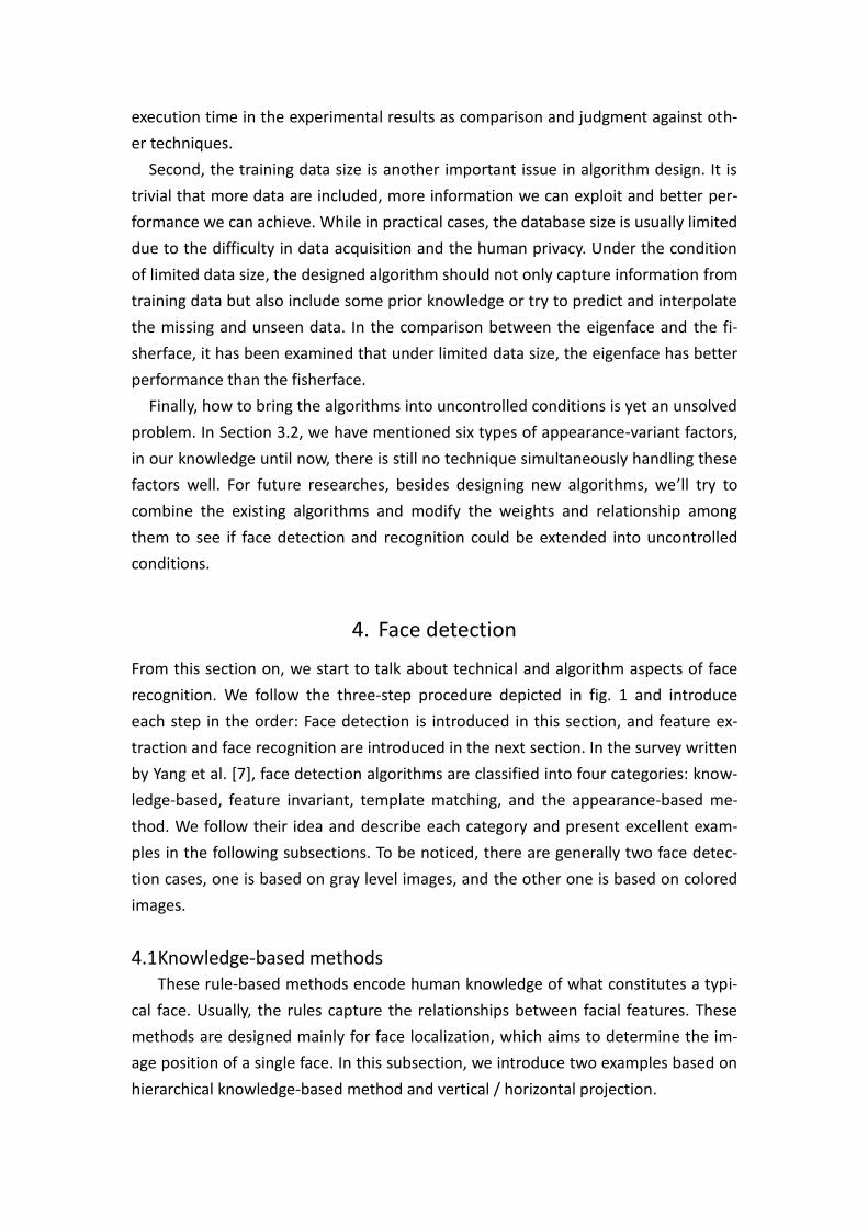
Figure 9: The multi-resolution hierarchy of images created by averaging and sub-sampling. (a) The

original image. (b) The image with each 4-by-4 square substituted by the averaged intensity of pixels

in that square. (c) The image with 8-by-8 square. (d) The image with 16-by-16 square. [7]

Figure 10: Examples of the horizontal / vertical projection method. The image (a) and image (b) are

sub-sampled with 8-by-8 squares by the same method described in fig. 7, and (c) with 4-by-4. The

projection method performs well in image (a) while can’t handle complicated backgrounds and mul-

ti-face images in image (b) and (c). [7]

4.1.1 Hierarchical knowledge-based method

This method is composed of the multi-resolution hierarchy of images and specific

rules defined at each image level [8]. The hierarchy is built by image sub-sampling

and an example is shown in fig. 9. The face detection procedure starts from the

highest layer in the hierarchy (with the lowest resolution) and extracts possible face

candidates based on the general look of faces. Then the middle and bottom layers

carry rule of more details such as the alignment of facial features and verify each face

candidate. This method suffers from many factors described in Section 3 especially

the RST variation and doesn’t achieve high detection rate (50 true positives in 60 test

images), while the coarse-to-fine strategy does reduces the required computation

and is widely adopted by later algorithms.

4.1.2 Horizontal / vertical projection

This method uses the fairly simple image processing technique, the horizontal

and vertical projection [9]. Based on the observations that human eyes and mouths

have lower intensity than other parts of faces, these two projections are performed

on the test image and local minimums are detected as facial feature candidates

which together constitute a face candidate. Finally, each face candidate is validated

by further detection rules such as eyebrow and nostrils. As shown in fig. 10, this me-

thod is sensitive to complicated backgrounds and can’t be used on images with mul-

tiple faces.

4.2 Feature invariant approaches These algorithms aim to find structural features that exist even when the pose,

viewpoint, or lighting conditions vary, and then use these to locate faces. These me-

thods are designed mainly for face localization. To distinguish from the know-

ledge-based methods, the feature invariant approaches start at feature extraction

process and face candidates finding, and later verify each candidate by spatial rela-

tions among these features, while the knowledge-based methods usually exploit in-

formation of the whole image and are sensitive to complicated backgrounds and

other factors described in Section 3. We present two characteristic techniques of this

category in the following subsections, and readers could find more works in

[6][12][13][14][26][27].

4.2.1 Face Detection Using Color Information

In this work, Hsu et al. [10] proposed to combine several features for face detec-

tion. They used color information for skin-color detection to extract candidate face

regions. In order to deal with different illumination conditions, they extracted the 5%

brightest pixels and used their mean color for lighting compensation. After skin-color

detection and skin-region segmentation, they proposed to detect invariant facial

features for region verification. Human eyes and mouths are selected as the most

significant features of faces and two detection schemes are designed based on

chrominance contrast and morphological operations, which are called “eyes map”

and “mouth map”. Finally, we form the triangle between two eyes and a mouth and

verify it based on (1) luminance variations and average gradient orientations of eye

and mouth blobs, (2) geometry and orientation of the triangle, and (3) the presence

of a face boundary around the triangle. The regions pass the verification are denoted

as faces and the Hough transform are performed to extract the best-fitting ellipse to

extract each face.

This work gives a good example of how to combine several different techniques

together in a cascade fashion. The lighting compensation process doesn’t have a sol-

id background, but it introduces the idea that despite modeling all kinds of illumina-

tion conditions based on complicated probability or classifier models, we can design

an illumination-adaptive model which modifies its detection threshold based on the

illumination and chrominance properties of the present image. The eyes map and

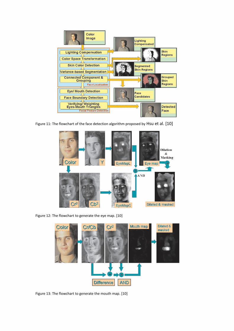
Figure 11: The flowchart of the face detection algorithm proposed by Hsu et al. [10]

Figure 12: The flowchart to generate the eye map. [10]

Figure 13: The flowchart to generate the mouth map. [10]

the mouth map shows great performance with fairly simple operations, and in our

recent work we also adopt their framework and try to design more robust maps.

4.2.2 Face detection based on random labeled graph matching Leung et al. developed a probabilistic method to locate a face in a cluttered scene

based on local feature detectors and random graph matching [11]. Their motivation

is to formulate the face localization problem as a search problem in which the goal is

to find the arrangement of certain features that is most likely to be a face pattern. In

the initial step, a set of local feature detectors is applied to the image to identify can-

didate locations for facial features, such as eyes, nose, and nostrils, since the feature

detectors are not perfectly reliable, the spatial arrangement of the features must also

be used for localize the face.

The facial feature detectors are built by the multi-orientation and multi-scale

Gaussian derivative filters, where we select some characteristic facial features (two

eyes, two nostrils, and nose/lip junction) and generate a prototype filter response for

each of them. The same filter operation is applied to the input image and we com-

pare the response with the prototype responses to detect possible facial features. To

enhance the reliability of these detectors, the multivariate-Gaussian distribution is

used to represent the distribution of the mutual distances among each facial feature,

and this distribution is estimated by a set of training arrangements. The facial feature

detectors averagely find 10-20 candidate locations for each facial feature, and the

brute-force matching for each possible facial feature arrangement is computationally

very demanding. To solve this problem, the authors proposed the idea of controlled

search. They set a higher threshold for strong facial feature detection, and each pair

of these strong features is selected to estimate the locations of other three facial

features using a statistical model of mutual distances. Furthermore, the covariance of

the estimates can be computed. Thus, the expected feature locations are estimated

with high probability and shown as ellipse regions as depicted in fig. 14. Constella-

tions are formed only from candidate facial features that lie inside the appropriate

locations, and the ranking of constellation is based on a probability density function

that a constellation corresponds to a face versus the probability it was generated by

the non-face mechanism. In their experiments, this system is able to achieve a cor-

rect localization rate of 86% for cluttered images.

This work presents how to estimate the statistical properties among characteristic

facial features and how to predict possible facial feature locations based on other

observed facial features. Although the facial feature detectors used in this work is not

robust compared to other detection algorithms, their controlled search scheme

could detect faces even some features are occluded.

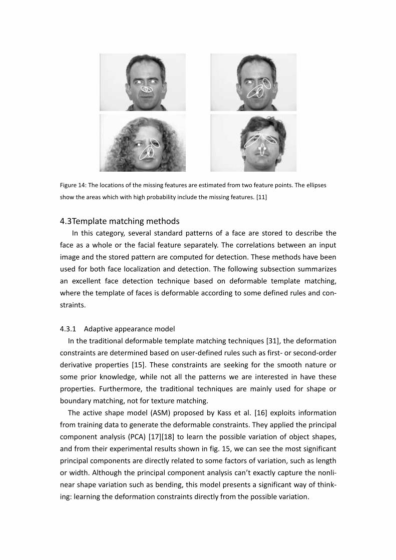
Figure 14: The locations of the missing features are estimated from two feature points. The ellipses

show the areas which with high probability include the missing features. [11]

4.3 Template matching methods In this category, several standard patterns of a face are stored to describe the

face as a whole or the facial feature separately. The correlations between an input

image and the stored pattern are computed for detection. These methods have been

used for both face localization and detection. The following subsection summarizes

an excellent face detection technique based on deformable template matching,

where the template of faces is deformable according to some defined rules and con-

straints.

4.3.1 Adaptive appearance model

In the traditional deformable template matching techniques [31], the deformation

constraints are determined based on user-defined rules such as first- or second-order

derivative properties [15]. These constraints are seeking for the smooth nature or

some prior knowledge, while not all the patterns we are interested in have these

properties. Furthermore, the traditional techniques are mainly used for shape or

boundary matching, not for texture matching.

The active shape model (ASM) proposed by Kass et al. [16] exploits information

from training data to generate the deformable constraints. They applied the principal

component analysis (PCA) [17][18] to learn the possible variation of object shapes,

and from their experimental results shown in fig. 15, we can see the most significant

principal components are directly related to some factors of variation, such as length

or width. Although the principal component analysis can’t exactly capture the nonli-

near shape variation such as bending, this model presents a significant way of think-

ing: learning the deformation constraints directly from the possible variation.

(a) (b)

(c) (d) (e)

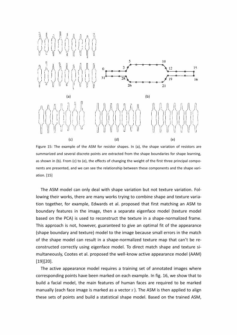
Figure 15: The example of the ASM for resistor shapes. In (a), the shape variation of resistors are

summarized and several discrete points are extracted from the shape boundaries for shape learning,

as shown in (b). From (c) to (e), the effects of changing the weight of the first three principal compo-

nents are presented, and we can see the relationship between these components and the shape vari-

ation. [15]

The ASM model can only deal with shape variation but not texture variation. Fol-

lowing their works, there are many works trying to combine shape and texture varia-

tion together, for example, Edwards et al. proposed that first matching an ASM to

boundary features in the image, then a separate eigenface model (texture model

based on the PCA) is used to reconstruct the texture in a shape-normalized frame.

This approach is not, however, guaranteed to give an optimal fit of the appearance

(shape boundary and texture) model to the image because small errors in the match

of the shape model can result in a shape-normalized texture map that can’t be re-

constructed correctly using eigenface model. To direct match shape and texture si-

multaneously, Cootes et al. proposed the well-know active appearance model (AAM)

[19][20].

The active appearance model requires a training set of annotated images where

corresponding points have been marked on each example. In fig. 16, we show that to

build a facial model, the main features of human faces are required to be marked

manually (each face image is marked as a vector x ). The ASM is then applied to align

these sets of points and build a statistical shape model. Based on the trained ASM,

each training face is warped so the points match those of the mean shape x , obtain-

ing a shape-free patch. These shape-free patches are further represented as a set of

vectors and undergo the intensity normalization process (each vector is denoted as

g ). By applying the PCA to the intensity normalized data we obtain a linear model

that captures the possible texture variation. We summarize the process that has

been done until now for the AAM as follows:

s s

g g

x x Pb

g g P b

, where sP is the orthonormal bases of the ASM and sb is the set of shape para-

meters for each training face. The matrix is the orthonormal bases of the texture

variation and is the set of texture parameters for each intensity normalized

shape-free patch. The details and process of the PCA is described in Section 5.

To capture the correlation between shape and texture variation, a further PCA is

applied to the data as follows. For each training example we generate the concate-

nated vector:

( )

( )

T

s s s s

Tg g

W b W P x xb

b P g g

, where sW is a diagonal matrix of weights for each shape parameter, allowing for

the difference in units between the shape and texture models. The PCA is applied on

these vectors to generate a further model:

b Qc

, where Q represents the eigenvectors and c is a vector of appearance parameters

controlling both the shape and texture of the model. Note that the linear nature of

the model allows us to express the shape and texture directly as function of c:

s s s

g g

s

g

x x PW Q c

g g P Q c

QQ

Q

An example image can be synthesized for a given c by generating the shape-free tex-

ture patch first and warp it to the suitable shape.

In the training phase for face detection, we learn the mean vectors of shape and

texture, sP , , sW , and Q to generate a facial AAM. And in the face detection phase,

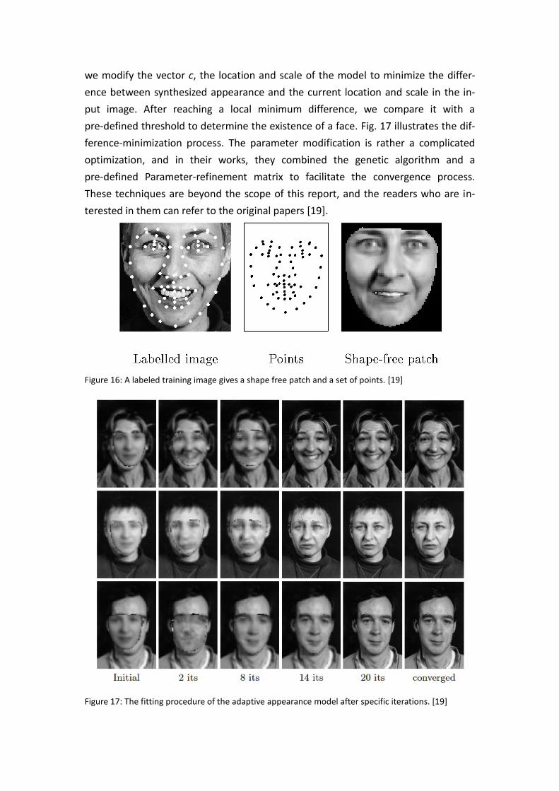
we modify the vector c, the location and scale of the model to minimize the differ-

ence between synthesized appearance and the current location and scale in the in-

put image. After reaching a local minimum difference, we compare it with a

pre-defined threshold to determine the existence of a face. Fig. 17 illustrates the dif-

ference-minimization process. The parameter modification is rather a complicated

optimization, and in their works, they combined the genetic algorithm and a

pre-defined Parameter-refinement matrix to facilitate the convergence process.

These techniques are beyond the scope of this report, and the readers who are in-

terested in them can refer to the original papers [19].

Figure 16: A labeled training image gives a shape free patch and a set of points. [19]

Figure 17: The fitting procedure of the adaptive appearance model after specific iterations. [19]

4.4 Appearance-based methods In contrast to template matching, the models (or templates) are learned from a set

of training images which should capture the representative variability of facial ap-

pearance. These learned models are then used for detection. These methods are de-

signed mainly for face detection, and two high-cited works are introduced in the fol-

lowing sections. More significant techniques are included in [7][24][25][26].

4.4.1 Example-based learning for view-based human face detection

The appearance-based methods consider not the facial feature points but all regions

of the face. Given a window size, the appearance-based method scans through the

image and analyze each covered region. In the work of Sung et al. [21], the window

size of 19x19 is selected for training and each extracted patch can be represented by

a 381-dimensional vector, which is shown in fig. 18. A face mask is used to disregard

pixels near the boundaries of the window which may contain background pixels, and

reduce the vector into 283 dimensions. In order to better capture the distribution of

the face samples, the Gaussian mixture model [28] is used. Given samples of face

patches and non-face patches, two six-component Gaussian mixture models are

trained based on the modified K-means algorithm [28]. The non-face patches need to

be carefully chosen in order to include non-face samples as many as possible, espe-

cially some naturally non-face patterns in the real world that look like faces when

viewed in a selected window. To classify a test patch, the distances between the

patch and the 12 trained components are extracted as the patch feature, and a mul-

tilayer neural network [29][30] is trained to capture the relationship between these

patch features and the corresponding labels.

During the face detection phase, several window sizes are selected to scan the input

image, where each extracted patches are first resized into size of 19x19. Then we

perform the mask operation, extract the patch features, and classify each patch into

face or non-face based on the neural network classifier.

4.4.2 Fast face detection based on the Haar features and the Adaboost algorithm

The appearance-based method usually has better performance than the fea-

ture-invariant because it scans all the possible locations and scales in the image, but

this exhaustive searching procedure also result in considerable computation. In order

to facilitate this procedure, Viola et al. [22][23] proposed the combination of the

Haar features and the Adaboost classifier [18][28]. The Haar features are used to

capture the significant characteristics of human faces, especially the contrast fea-

tures. Fig. 19 shows the adopted four feature shapes, where each feature is labeled

by its width, length, type, and the contrast value (which is calculated as the averaged

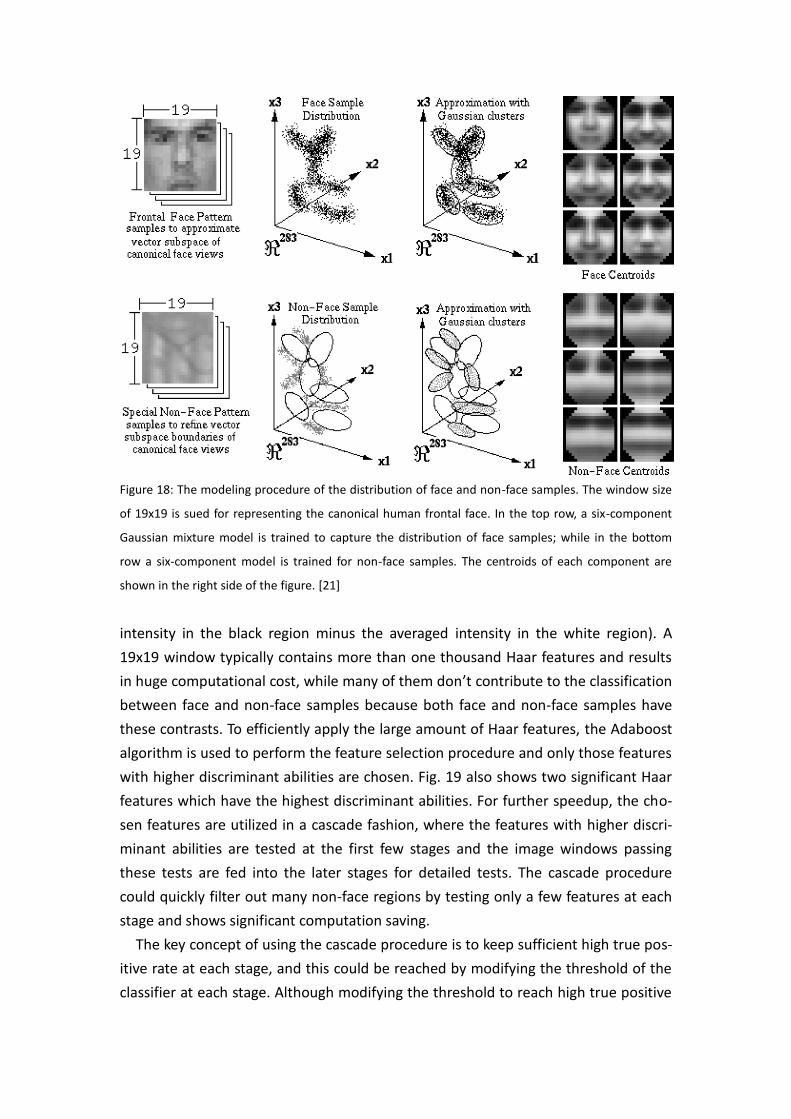
Figure 18: The modeling procedure of the distribution of face and non-face samples. The window size

of 19x19 is sued for representing the canonical human frontal face. In the top row, a six-component

Gaussian mixture model is trained to capture the distribution of face samples; while in the bottom

row a six-component model is trained for non-face samples. The centroids of each component are

shown in the right side of the figure. [21]

intensity in the black region minus the averaged intensity in the white region). A

19x19 window typically contains more than one thousand Haar features and results

in huge computational cost, while many of them don’t contribute to the classification

between face and non-face samples because both face and non-face samples have

these contrasts. To efficiently apply the large amount of Haar features, the Adaboost

algorithm is used to perform the feature selection procedure and only those features

with higher discriminant abilities are chosen. Fig. 19 also shows two significant Haar

features which have the highest discriminant abilities. For further speedup, the cho-

sen features are utilized in a cascade fashion, where the features with higher discri-

minant abilities are tested at the first few stages and the image windows passing

these tests are fed into the later stages for detailed tests. The cascade procedure

could quickly filter out many non-face regions by testing only a few features at each

stage and shows significant computation saving.

The key concept of using the cascade procedure is to keep sufficient high true pos-

itive rate at each stage, and this could be reached by modifying the threshold of the

classifier at each stage. Although modifying the threshold to reach high true positive

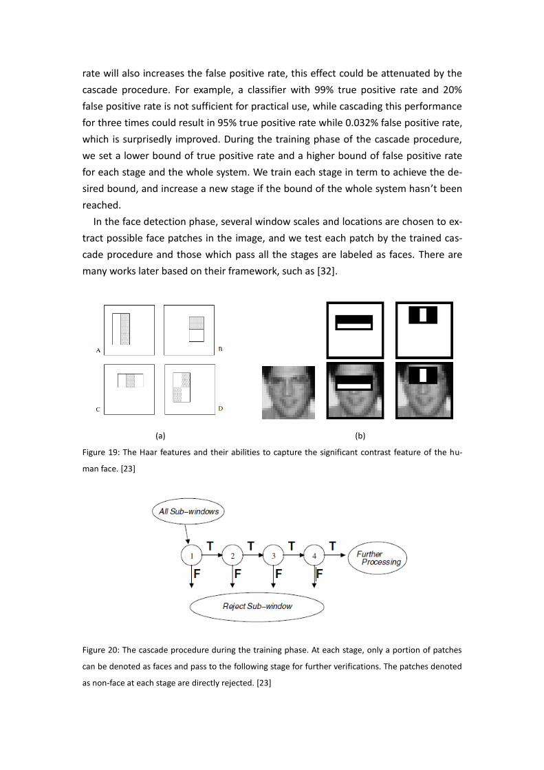
rate will also increases the false positive rate, this effect could be attenuated by the

cascade procedure. For example, a classifier with 99% true positive rate and 20%

false positive rate is not sufficient for practical use, while cascading this performance

for three times could result in 95% true positive rate while 0.032% false positive rate,

which is surprisedly improved. During the training phase of the cascade procedure,

we set a lower bound of true positive rate and a higher bound of false positive rate

for each stage and the whole system. We train each stage in term to achieve the de-

sired bound, and increase a new stage if the bound of the whole system hasn’t been

reached.

In the face detection phase, several window scales and locations are chosen to ex-

tract possible face patches in the image, and we test each patch by the trained cas-

cade procedure and those which pass all the stages are labeled as faces. There are

many works later based on their framework, such as [32].

(a) (b)

Figure 19: The Haar features and their abilities to capture the significant contrast feature of the hu-

man face. [23]

Figure 20: The cascade procedure during the training phase. At each stage, only a portion of patches

can be denoted as faces and pass to the following stage for further verifications. The patches denoted

as non-face at each stage are directly rejected. [23]

4.5 Part-based methods With the development of the graphical model framework [33] and the point of inter-

est detection such as the difference of Gaussian detector [34] (used in the SIFT de-

tector) and the Hessian affine detector [35], the part-based method recently attracts

more attention. We’d like to introduce two outstanding examples, one is based on

the generative model and one is based on the support vector machine (SVM) classifi-

er.

4.5.1 Face detection based on the generative model framework

R. Fergus et al. [36] proposed to learn and recognize the object models from unla-

beled and unsegmented cluttered scenes in a scale invariant manner. Objects are

modeled as flexible constellations of parts, and only the topic of each image should

be given (for example, car, people, or motors, etc.). The object model is generated by

the probabilistic representation and each object is denoted by the parts detected by

the entropy-based feature detector. Aspects including appearances, scales, shapes,

and occlusions of each part and the object are considered and modeled by the

probabilistic representation to deal with possible object variances.

Given an image, the entropy-based feature detector is first applied to detect the

top P parts (including locations and scales) with the largest entropies, and then these

parts are fed into the probabilistic model for object recognition. The probabilistic

object model is composed of N interesting parts (N<P) and denoted as follows:

(Object | , , ) ( , , | Object) (Object)

(No object | , , ) ( , , | No object) (No object)

( , , | ) (Object)

( , , | ) (No object)bg

p X S A p X S A pR

p X S A p X S A p

p X S A p

p X S A p

Appearance Shape Rel. scale Other

( , , | ) ( , , , | )

( | , , , ) ( | , , ) ( | , ) ( | )

h H

h H

p X S A p X S A h

p A X S h p X S h p S h p h

, where X denotes the part locations, S denotes the scales, and A denotes the ap-

pearances. The indexing variable h is a hypothesis to determine the attribute of each

detected part (belong to the N interesting parts of the object or not) and the possible

occlusion of each interesting part (If no detected part is assigned to an interesting

part, this interesting part is occluded in the image). Note that P regions are detected

from the image while we assume that only N points are characteristics of the object

and other parts belong to the background.

The model is trained by the well-known expectation maximization (EM) algorithm

[28] in order to cope with the unobserved variable h, and both the object model and

background model are trained from the same set of object-labeled images. Then

when an input image comes in, we first extract its P parts and calculate the quantity

R. Comparing this R with a defined threshold, we can determine if there is any face

appears in the image. In addition to this determination, we can analyze each h and

extract the N interesting parts of this image according to h with the highest probabil-

ity score. From fig. 21, we see that these detected N parts based on the highest score

h actually capture the meaningful characteristics of human faces.

Figure 21: An example of face detection based on the generative model framework. (Up-left) The av-

eraged location and the location variance of each interesting part of the face. (Up-right) Sample ap-

pearances of the six interesting parts and the background part (the bottom row). (Bottom) Examples

of faces and the corresponding interesting parts. [36]

4.5.2 Component-based face detection based on the SVM classifier

Based on the same idea of using detected parts to represent human faces, Bernd et

al. [37] proposed the face detection algorithm consisting of a two-level hierarchy of

support vector machine (SVM) classifiers [18][28]. On the first level, component clas-

sifiers independently detect components of a face. On the second level, a single clas-

sifier checks if the geometrical configuration of the detected components in the im-

age matches a geometrical model of a face. Fig. 22 shows the procedure of their al-

gorithm.

On the first level, the linear SVM classifiers are trained to detect each component.

Rather than manually extracting each component from training images, the authors

proposed an automatic algorithm to select components based on their discrimina-

tive power and their robustness against pose and illumination changes (in their im-

plementation, 14 components are used). This algorithm starts with a small rectangu-

lar component located around a pre-selected point in the face. In order to simplify

the training phase, the authors used synthetic 3D images for component learning.

The component is extracted from all synthetic face images to build a training set of

positive examples, and a training set of non-face pattern that have that same rec-

tangular shape is also generated. After training an SVM on the component data, they

estimate the performance of the SVM based on the estimated upper bound on

the expected probability of error and later the component is enlarged by expanding

the rectangle by one pixel into one of the four directions (up, down, left, right). Again,

they generated training data, trained an SVM, determined , and finally kept the

expansion which decreases the most. This process is continued until the expan-

sions into all four directions lead to an increase in , and the SVM classifier of the

component is determined.

On the second level the geometrical configuration classifier performs the final face

detection by linear combining the results of the component classifiers. Given a

window (a current face searching window), the maximum continuous out-

puts of the component classifiers within rectangular search regions around the ex-

pected positions of the components and the detected positions are used as inputs to

the geometrical configuration classifier. The search regions have been calculated

from the mean and standard deviation of the locations of the components in the

training images. The output of this second-level SVM tells us if a face is detected in

the current window. To search all possible scales and locations inside an

input image, we need to change the window sizes of each component and possible

face size, which is an exhaustive process.

In their work, they proposed three basic ideas behind part- or component-based

detection of objects. First, some object classes can be described well by a few cha-

racteristic object parts and their geometrical relation. Second, the patterns of some

object parts might vary less under pose changes than the pattern belonging to the

whole object. Third, a component-based approach might be more robust against

partial occlusions than a global approach. And the two main problems of a compo-

nent-based approach are how to choose the set of discriminatory object parts and

how to model their geometrical configuration.

(a) (b)

Fig 22: In (a), the system overview of the component-based classifier using four components is pre-

sented. On the first level, windows of the size of the components (solid line boxes) are shifted over the

face image and classified by the component classifiers. On the second, the maximum outputs of the

component classifiers within predefined search regions (dotted lined boxes) and the positions of the

components are fed into the geometrical configuration classifier. In (b), the fourteen learned compo-

nents are denoted by the black boxes with the corresponding center marked by crosses. [37]

4.6 Our proposed methods

(a) (b)

Figure 23: (a) The input image and the result after skin-color detection. (b) The extracted connected

patch and its most fitted ellipse.

(a) (b)

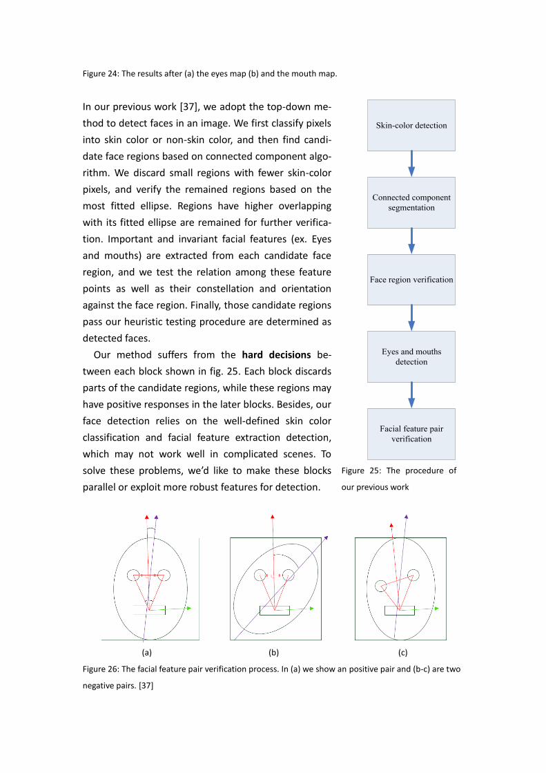
Figure 24: The results after (a) the eyes map (b) and the mouth map.

In our previous work [37], we adopt the top-down me-

thod to detect faces in an image. We first classify pixels

into skin color or non-skin color, and then find candi-

date face regions based on connected component algo-

rithm. We discard small regions with fewer skin-color

pixels, and verify the remained regions based on the

most fitted ellipse. Regions have higher overlapping

with its fitted ellipse are remained for further verifica-

tion. Important and invariant facial features (ex. Eyes

and mouths) are extracted from each candidate face

region, and we test the relation among these feature

points as well as their constellation and orientation

against the face region. Finally, those candidate regions

pass our heuristic testing procedure are determined as

detected faces.

Our method suffers from the hard decisions be-

tween each block shown in fig. 25. Each block discards

parts of the candidate regions, while these regions may

have positive responses in the later blocks. Besides, our

face detection relies on the well-defined skin color

classification and facial feature extraction detection,

which may not work well in complicated scenes. To

solve these problems, we’d like to make these blocks

parallel or exploit more robust features for detection.

Skin-color detection

Connected component

segmentation

Face region verification

Eyes and mouths

detection

Facial feature pair

verification

Figure 25: The procedure of

our previous work

(a) (b) (c)

Figure 26: The facial feature pair verification process. In (a) we show an positive pair and (b-c) are two

negative pairs. [37]

5. Feature Extraction and Face Recognition

Assumed that the face of a person is located, segmented from the image, and aligned

into a face patch, in this section, we’ll talk about how to extract useful and compact

features from face patches. The reason to combine feature extraction and face rec-

ognition steps together is that sometimes the type of classifier is corresponded to

the specific features adopted. In this section, we separate the feature extraction

techniques into four categories: holistic-based method, feature-based method, tem-

plate-based method, and part-based method. The first three categories are fre-

quently discussed in literatures, while the forth category is a new idea used in recent

computer vision and object recognition.

5.1 Holistic-based methods Holistic-based methods are also called appearance-based methods, which mean we

use whole information of a face patch and perform some transformation on this

patch to get a compact representation for recognition. To be more clearly distin-

guished from feature-based methods, we can say that feature-based methods di-

rectly extract information from some detected fiducial points (such as eyes, noses,

and lips, etc. These fiducial points are usually determined from domain knowledge)

and discard other information; while appearance-based methods perform transfor-

mations on the whole patch and reach the feature vectors, and these transformation

basis are usually obtained from statistics.

During the past twenty years, holistic-based methods attract the most attention

against other methods, so we will focus more on this category. In the following sub-

sections, we will talk about the famous eigenface [39] (performed by the PCA), fi-

sherface (performed by the LDA), and some other transformation basis such as the

independent component analysis (ICA), nonlinear dimension reduction technique,

and the over-complete database (based on compressive sensing). More interesting

techniques could be found in [42][43].

5.1.1 Eigenface and Principal Component Analysis

The idea of eigenface is rather easy. Given a face data set (say N faces), we first scale

each face patch into a constant size (for example, 100x100) and transfer each patch

into vector representation (100-by-100 matrix into 10000-by-1 vector). Based on

these N D-dimensional vectors (D=10000 in this case), we can apply the principal

component analysis (PCA) [17][18] to obtain suitable basis (each is a D-dimensional

vector) for dimension reduction. Assume we choose M projection basis ( ),

each D-dimensional vector could be transformed into an M-dimensional vector re-

presentation. Generally, these M projection basis are called eigenfaces. The algo-

rithms for PCA and eigenfaces representation are shown below:

Eigenface representation:

(1) Initial setting:

Originally N D-dimensional vectors:

A set of M projection basis:

These basis are mutually orthogonal, and generally we have

(2) The eigenface representation

For each (i=1~N), we compute its projection onto , and

we can get a new M-dimensional vector . This process achieves our goal

of dimension reduction.

The PCA basis:

PCA projection basis are purely data-driven, which are computed from the dataset

we have. This projection process is also called Karhunen-Loeve transform in the

data compression community. Given N D-dimensional vectors (In face recognition

task, usually ), we can get at least min(N-1, D-1) projection basis with one

mean vector:

(1) Compute the mean vector Ψ (D-by-1 vector)

(2) Subtract each by Ψ and get

(3) Calculate the covariance matrix Σ of all the s (D-by-D matrix)

(4) Calculate the set of Σ (D-by-(N-1) matrix, where each eigenvector is aligned as a column vector)

(5) Preserve the M largest eigenvectors based on their eigenvalues (D-by-M matrix U)

(6) is the eigenface representation (M-dimensional vector) of the ith face

The orthogonal PCA bases are proved to preserve the most projection energy and

preserve the largest variation after projection, while the proof is not included in this

report. In the work proposed by Turk et al., they proposed a speed-up algorithm to

reach the eigenvectors form the covariance matrix Σ, and used the vectors after

dimension reduction for face detection and face recognition. They also proposed

some criteria for face detection and face tracking.

The PCA method has been proved to discard noise and outlier data from the

training set, while they may also ignore some key discriminative factors which may

not have large variation but dominate our perception. We’ll compare this effect in

the next subsection about the fisherface and linear discriminant analysis. To be

announced, the eigenface algorithm did give significant influences on the algorithm

design for holistic-based face recognition in the past twenty years, so it is a great

starting point for readers to try building a face recognition system.

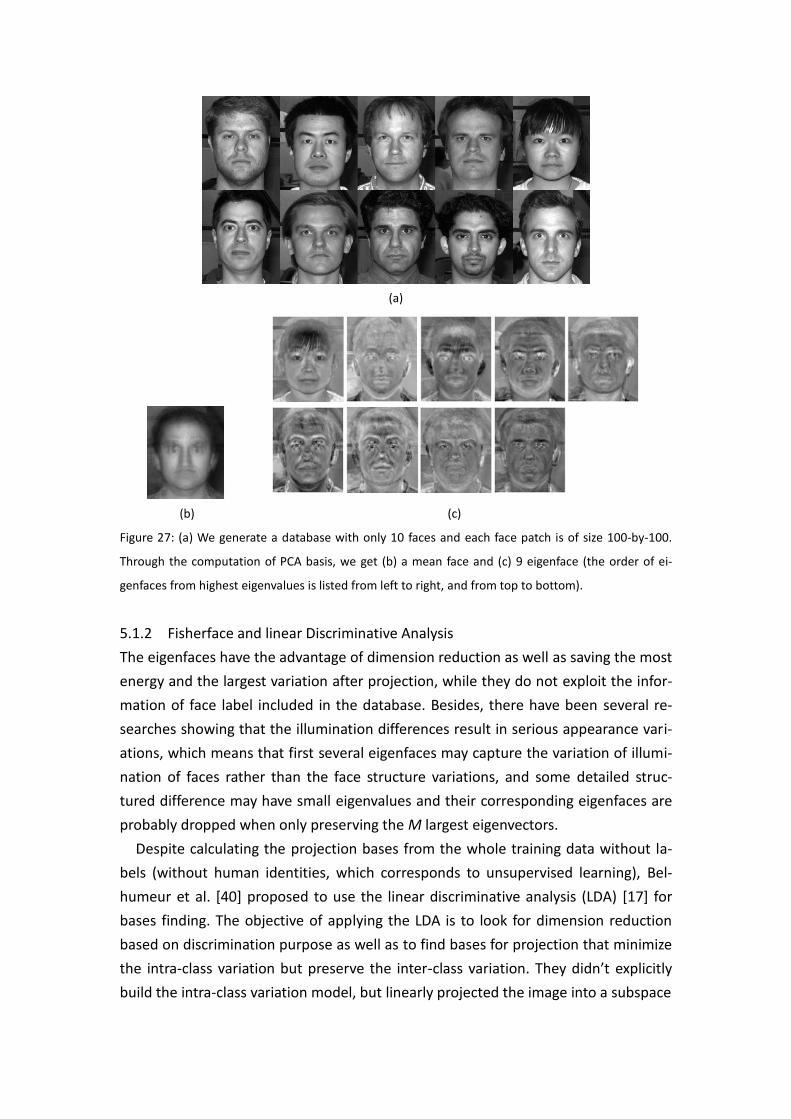
(a)

(b) (c)

Figure 27: (a) We generate a database with only 10 faces and each face patch is of size 100-by-100.

Through the computation of PCA basis, we get (b) a mean face and (c) 9 eigenface (the order of ei-

genfaces from highest eigenvalues is listed from left to right, and from top to bottom).

5.1.2 Fisherface and linear Discriminative Analysis

The eigenfaces have the advantage of dimension reduction as well as saving the most

energy and the largest variation after projection, while they do not exploit the infor-

mation of face label included in the database. Besides, there have been several re-

searches showing that the illumination differences result in serious appearance vari-

ations, which means that first several eigenfaces may capture the variation of illumi-

nation of faces rather than the face structure variations, and some detailed struc-

tured difference may have small eigenvalues and their corresponding eigenfaces are

probably dropped when only preserving the M largest eigenvectors.

Despite calculating the projection bases from the whole training data without la-

bels (without human identities, which corresponds to unsupervised learning), Bel-

humeur et al. [40] proposed to use the linear discriminative analysis (LDA) [17] for

bases finding. The objective of applying the LDA is to look for dimension reduction

based on discrimination purpose as well as to find bases for projection that minimize

the intra-class variation but preserve the inter-class variation. They didn’t explicitly

build the intra-class variation model, but linearly projected the image into a subspace

(a)

(b)

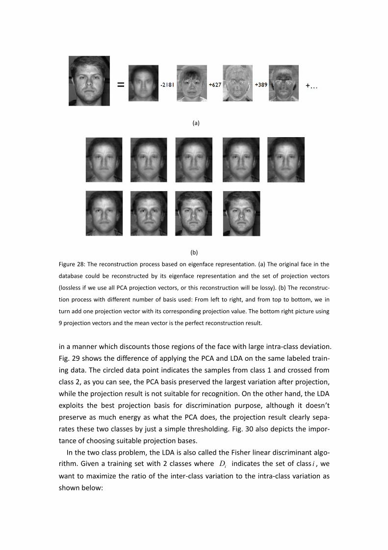
Figure 28: The reconstruction process based on eigenface representation. (a) The original face in the

database could be reconstructed by its eigenface representation and the set of projection vectors

(lossless if we use all PCA projection vectors, or this reconstruction will be lossy). (b) The reconstruc-

tion process with different number of basis used: From left to right, and from top to bottom, we in

turn add one projection vector with its corresponding projection value. The bottom right picture using

9 projection vectors and the mean vector is the perfect reconstruction result.

in a manner which discounts those regions of the face with large intra-class deviation.

Fig. 29 shows the difference of applying the PCA and LDA on the same labeled train-

ing data. The circled data point indicates the samples from class 1 and crossed from

class 2, as you can see, the PCA basis preserved the largest variation after projection,

while the projection result is not suitable for recognition. On the other hand, the LDA

exploits the best projection basis for discrimination purpose, although it doesn’t

preserve as much energy as what the PCA does, the projection result clearly sepa-

rates these two classes by just a simple thresholding. Fig. 30 also depicts the impor-

tance of choosing suitable projection bases.

In the two class problem, the LDA is also called the Fisher linear discriminant algo-

rithm. Given a training set with 2 classes where iD indicates the set of class i , we

want to maximize the ratio of the inter-class variation to the intra-class variation as

shown below:

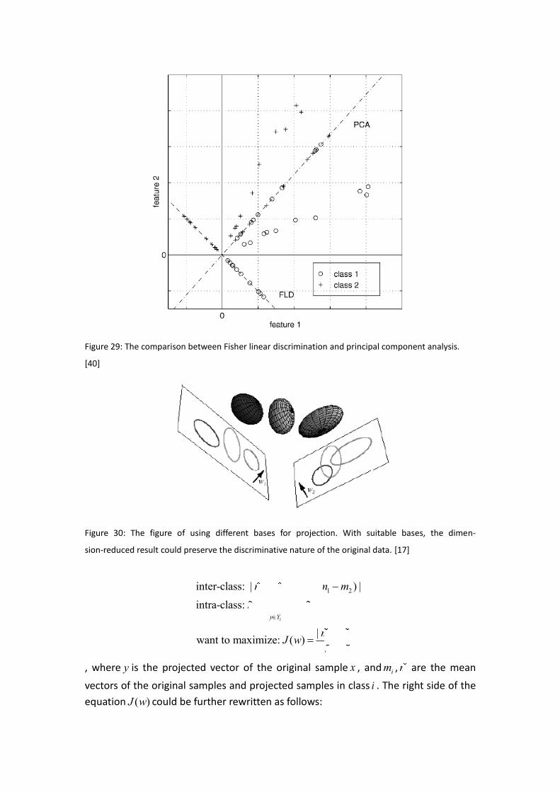
Figure 29: The comparison between Fisher linear discrimination and principal component analysis.

[40]

Figure 30: The figure of using different bases for projection. With suitable bases, the dimen-

sion-reduced result could preserve the discriminative nature of the original data. [17]

T

1 2 1 2

2 2

2

1 2

2 2

1 2

inter-class: | | | ( ) |

intra-class: ( )

| |want to maximize: ( )

i

i i

y Y

m m w m m

s y m

m mJ w

s s

, where y is the projected vector of the original sample x , and im , im are the mean

vectors of the original samples and projected samples in class i . The right side of the

equation ( )J w could be further rewritten as follows:

2 T T T T T T T T

2 2 T T T

1 2 1 2 w

2 T T 2 T T T

1 2 1 2 1 2 1 2 B

T

B

T

w

( )( ) ( )( )

| | ( ) ( )( )

want to maximize: ( )

i i

i i i i i i

x D x D

s w x w m w x w m w x m x m w w S w

s s w S w w S w w S w

m m w m w m w m m m m w w S w

w S wJ w

w S w

, where the w means the projection vector here to be calculated and iD is the training

set of class i . This obtained ( )J w is well known in mathematical physics as the ge-

neralized Rayleigh quotient, and a vector w that maximizes ( )J w must satisfy

B wS w S w

for some constant , which is a generalized eigenvalues problem. If the wS is nonsin-

gular we can obtain a conventional eigenvalues problem by writing:

1

w BS S w w

And if wS is nonsingular, we can choose either pre-reducing the dimensionality of x by

the PCA or finding the bases from the nullspace of wS .

To solve the multiclass problem, given a training set with C classes, the intra-class

variation and inter-class variation could be rewritten as:

T

B

1

T

w

1

T

B

T

w

( )( )

( )( )

| |want to maximize: ( )

| |

i

c

i i i

i

c

i i

i x D

S N m m m m

S x m x m

W S WJ W

W S W

, where m is the mean vector of all the samples in the training set. W is the projec-

tion matrix where 1 2 m[ ...... ] W w w w with 1m c , and each iw should satisfy

B wi i iS w S w

In order to deal with the singularity problem of wS , Belhumeur et al. used the PCA

method described as below, where all the samples x in the training data are first pro-

jected to an dimension-reduced space, and BS , wS , andW are calculate in this space:

T T

PCA T T

T T

PCA B PCAFLD T T

PCA w PCA

arg max | | where ( )( )

| |arg max

| |

Wx

W

W W S W S x m x m

W W S W WW

W W S W W

ThewS has the maximum rank as N-C, where N is the size of the training set, so we

need to reduce the dimensionality of the samples x down to N-C or less. In their ex-

periment results, the LDA bases outperform the PCA bases, especially in the illumina-

tion changing cases. The LDA could also be applied in other recognition cases. For

example, fig.31 shows the projection basis for the glasses / without glasses case, and

as you can see, this basis capture the glass shape around human eyes, rather than

the face difference of people in the training set.

(a) (b)

Figure 31: The recognition case of human faces with glasses or without glasses. (a) an example of fac-

es with glasses. (b) the projection basis reached by the LDA. [40]

5.1.3 Independent Component Analysis

Followed the projection and bases finding ideas, the following three subsections use

different criteria to find the bases or decomposition of the training set. Because

these criteria involve many mathematical and statistical theorems and backgrounds,

here we will briefly describe the ideas behind them but no more details about the

mathematical equation and theorems.

The PCA exploits the second-order statistical property of the training set (the cova-

riance matrix) and yields projection bases that make the projected samples uncorre-

lated with each other. The second-order property only depends on the pair-wise re-

lationships between pixels, while some important information for face recognition

may be contained in the higher-order relationships among pixels. The independent

component analysis (ICA) [18][31] is a generalization of the PCA, which is sensitive to

the higher-order statistics. Fig. 32 shows the difference of the PCA bases and ICA

bases.

In the works proposed by Bartlett et al. [44], they derived the ICA bases from the

principle of optimal information transfer through sigmoidal neurons. In addition,

they proposed to architectures for dimension-reduction decomposition, one treats

the image as random variables and the pixels as outcomes, and the other one treats

the

Figure 32: (top) Example 3-D data distribution and corresponding PC and IC axes. Each axis is a column

of the projection matrix W found by the PCA and the ICA. Note that PC axes are orthogonal while the

ICA axes are not. IF only two components are allowed, the ICA choose a different subspace than ICA.

(bottom left) Distribution of the first PCA coordinates of the data. (bottom right) Distribution if the

first ICA coordinates of the data. Note that since the ICA axes are non-orthogonal, relative distance

between points are different in the PCA than in the ICA, as are the angels between points. As you can

see, the bases found by ICA preserve more original structure than the PCA. [44]

pixels as random variables and the image as outcomes. The Architecture I depicted in

fig. 33 found n “source of pixel” images, where each has the appearance as shown in

the column U illustrated in fig. 34, and a human face could be decomposed in to a

weight vector as in fig. 35. This architecture finds a set of statistically independent

basis images and each of them captures the features in human faces such as eyes,

eyebrows, and mouths.

The Architecture II finds the basis images which have similar appearances as the

PCA does as shown in fig. 36, and has the decomposition as shown in fig. 37. This ar-

chitecture uses the ICA to find a representation in which the coefficients used to

code images are statistically independent. Generally speaking, the first architectural

finds spatially local basis images for the face, while the second architecture produces

a factorial face code. In their experimental results, both these two representation

were superior to the representation based on the PCA for recognizing faces across

days and changes in expression, and a classifier combining these two ICA representa-

tion gave the best performance.

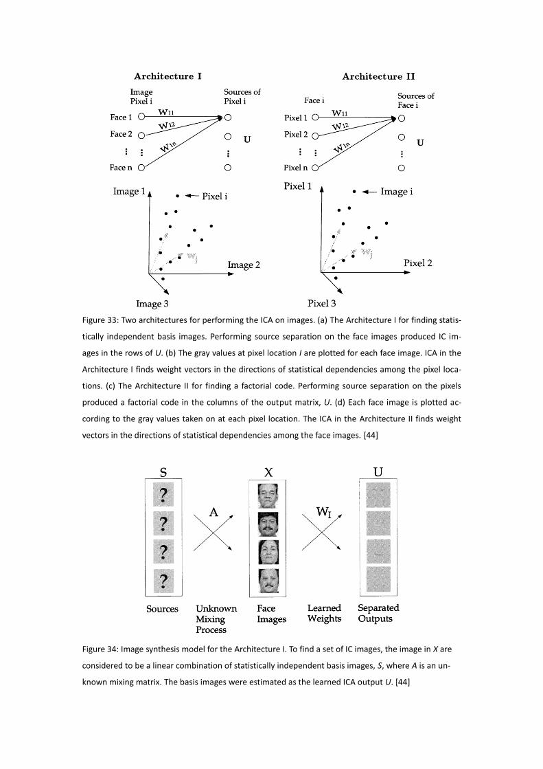
Figure 33: Two architectures for performing the ICA on images. (a) The Architecture I for finding statis-

tically independent basis images. Performing source separation on the face images produced IC im-

ages in the rows of U. (b) The gray values at pixel location I are plotted for each face image. ICA in the

Architecture I finds weight vectors in the directions of statistical dependencies among the pixel loca-

tions. (c) The Architecture II for finding a factorial code. Performing source separation on the pixels

produced a factorial code in the columns of the output matrix, U. (d) Each face image is plotted ac-

cording to the gray values taken on at each pixel location. The ICA in the Architecture II finds weight

vectors in the directions of statistical dependencies among the face images. [44]

Figure 34: Image synthesis model for the Architecture I. To find a set of IC images, the image in X are

considered to be a linear combination of statistically independent basis images, S, where A is an un-

known mixing matrix. The basis images were estimated as the learned ICA output U. [44]

Figure 35: The independent basis image representation consisted of the coefficients, b, for the linear

combination if independent basis images, u, that comprised each face image x. [44]

Figure 36: Image synthesis model for the Architecture II. Each image in the dataset was considered to

be a linear combination if underlying basis images in the matrix A. The basis images were each asso-

ciated with a set of independent “causes,” given by a vector of coefficients S. The basis images were

estimated by 1

IA W , where W is the learned ICA weight matrix. [44]

Figure 37: The factorial code representation consisted of the independent coefficients, u, for the linear

combination of basis images in A that comprised each face image x. [44]

5.1.4 Laplacianfaces and nonlinear dimension reduction

Despite using linear projection to obtain the representation vector of each face im-

age, some researchers claim that the nonlinear projection may yield better repre-

sentation for face recognition. The Laplacianfaces proposed by He et al. [45] used the

locality preserving projections (LPP) [46] to find an embedding that preserves local

information, and obtains a face subspace that best detects the essential face mani

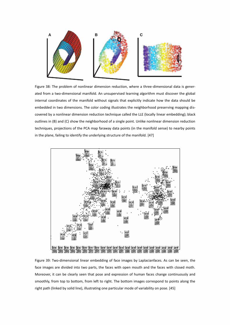
Figure 38: The problem of nonlinear dimension reduction, where a three-dimensional data is gener-

ated from a two-dimensional manifold. An unsupervised learning algorithm must discover the global

internal coordinates of the manifold without signals that explicitly indicate how the data should be

embedded in two dimensions. The color coding illustrates the neighborhood preserving mapping dis-

covered by a nonlinear dimension reduction technique called the LLE (locally linear embedding); black

outlines in (B) and (C) show the neighborhood of a single point. Unlike nonlinear dimension reduction

techniques, projections of the PCA map faraway data points (in the manifold sense) to nearby points

in the plane, failing to identify the underlying structure of the manifold. [47]

Figure 39: Two-dimensional linear embedding of face images by Laplacianfaces. As can be seen, the

face images are divided into two parts, the faces with open mouth and the faces with closed moth.

Moreover, it can be clearly seen that pose and expression of human faces change continuously and

smoothly, from top to bottom, from left to right. The bottom images correspond to points along the

right path (linked by solid line), illustrating one particular mode of variability on pose. [45]

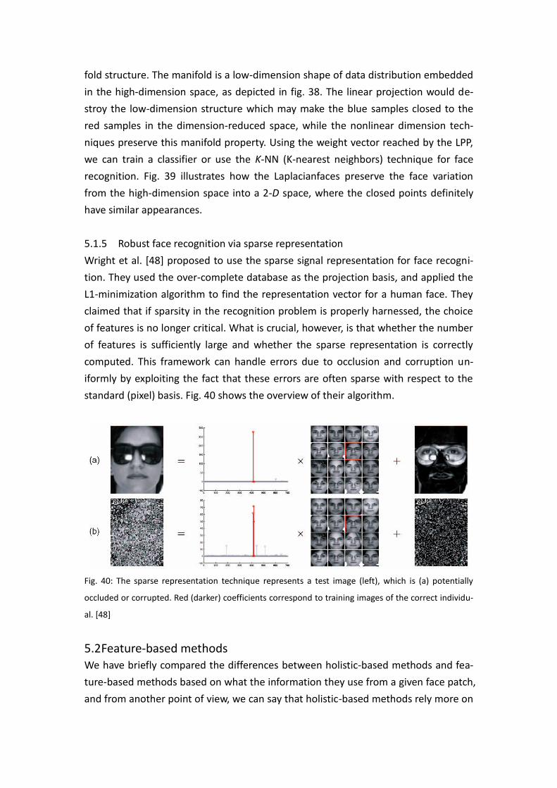
fold structure. The manifold is a low-dimension shape of data distribution embedded

in the high-dimension space, as depicted in fig. 38. The linear projection would de-

stroy the low-dimension structure which may make the blue samples closed to the

red samples in the dimension-reduced space, while the nonlinear dimension tech-

niques preserve this manifold property. Using the weight vector reached by the LPP,

we can train a classifier or use the K-NN (K-nearest neighbors) technique for face

recognition. Fig. 39 illustrates how the Laplacianfaces preserve the face variation

from the high-dimension space into a 2-D space, where the closed points definitely

have similar appearances.

5.1.5 Robust face recognition via sparse representation

Wright et al. [48] proposed to use the sparse signal representation for face recogni-

tion. They used the over-complete database as the projection basis, and applied the

L1-minimization algorithm to find the representation vector for a human face. They

claimed that if sparsity in the recognition problem is properly harnessed, the choice

of features is no longer critical. What is crucial, however, is that whether the number

of features is sufficiently large and whether the sparse representation is correctly

computed. This framework can handle errors due to occlusion and corruption un-

iformly by exploiting the fact that these errors are often sparse with respect to the

standard (pixel) basis. Fig. 40 shows the overview of their algorithm.

Fig. 40: The sparse representation technique represents a test image (left), which is (a) potentially

occluded or corrupted. Red (darker) coefficients correspond to training images of the correct individu-

al. [48]

5.2 Feature-based methods We have briefly compared the differences between holistic-based methods and fea-

ture-based methods based on what the information they use from a given face patch,

and from another point of view, we can say that holistic-based methods rely more on

statistical learning and analysis, while feature-based methods exploit more ideas

from image processing, computer vision, and domain knowledge form human. In this

section, we discus two outstanding features for face recognition, the Gabor wavelet

feature and the local binary pattern.

5.2.1 Gabor wavelet features with elastic graph matching based methods

The application of Gabor wavelet for face recognition is pioneered by Lades et al.’s

work [49]. In their work, the elastic graph matching framework is used for finding

feature points, building the face model and performing distance measurement, while

the Gabor wavelets are used to extract local features at these feature points, and a set

of complex Gabor wavelet coefficients for each point is called a jet. Graph matching

based methods normally requires two stages to build the graph for a face image I

and compute its similarity with a model graph . During the first stage, is

shifted within the input image to find the optimal global offset of while keeping

its shape rigid. Then in the second stage, each vertex in is shifted in a topological

constraint to compensate the local distortions due to rotations in depth or expression

variations. It is actually the deformation of the vertices that makes the graph matching

procedure elastic. To achieve these two stages, a cost measure function S( ) is

neccesarily to be defined and these two stages terminate when this function reaches

the minimum value.

Lades et al.’s [49] used a simple rectangular graph to model faces in the database

while each vertex is without the direct object meaning on faces. In the database

building stage, the deformation process mentioned above is not included, and the rec-

tangular graph is manually placed on each face and the features are extracted at indi-

vidual vertices. When a new face I comes in, the distance between it and all the faces

in the database are required to compute, which means if there are totally N face mod-

els in the database, we have to build N graphs for I based on each face model. This

matching process is very computationally expensive especially for large data-

base.Fig.41 shows an example of a model graph and a deformed graph based on it,

and the cost function is defined as:

where determines the relative importance of jet similarity and the topography term.

is the distance vector of the labeled edge e between two vertices, is the set of

jets at vertex n, and is the distance measure function between two jets based on

the magnitude of jets.

Wiskott et al. [50] proposed an improved elastic graph matching framework to

deal with the computational-expensive problem above and enhance the performance.

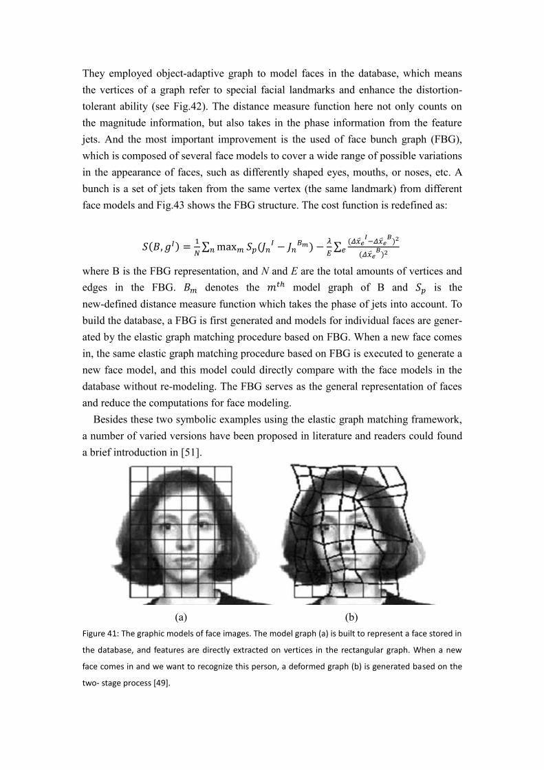
They employed object-adaptive graph to model faces in the database, which means

the vertices of a graph refer to special facial landmarks and enhance the distortion-

tolerant ability (see Fig.42). The distance measure function here not only counts on

the magnitude information, but also takes in the phase information from the feature

jets. And the most important improvement is the used of face bunch graph (FBG),

which is composed of several face models to cover a wide range of possible variations

in the appearance of faces, such as differently shaped eyes, mouths, or noses, etc. A

bunch is a set of jets taken from the same vertex (the same landmark) from different

face models and Fig.43 shows the FBG structure. The cost function is redefined as:

where B is the FBG representation, and N and E are the total amounts of vertices and

edges in the FBG. denotes the model graph of B and is the

new-defined distance measure function which takes the phase of jets into account. To

build the database, a FBG is first generated and models for individual faces are gener-

ated by the elastic graph matching procedure based on FBG. When a new face comes

in, the same elastic graph matching procedure based on FBG is executed to generate a

new face model, and this model could directly compare with the face models in the

database without re-modeling. The FBG serves as the general representation of faces

and reduce the computations for face modeling.

Besides these two symbolic examples using the elastic graph matching framework,

a number of varied versions have been proposed in literature and readers could found

a brief introduction in [51].

(a) (b)

Figure 41: The graphic models of face images. The model graph (a) is built to represent a face stored in

the database, and features are directly extracted on vertices in the rectangular graph. When a new

face comes in and we want to recognize this person, a deformed graph (b) is generated based on the

two- stage process [49].

Figure 42: The object-adaptive grids for difference poses. Now the vertices are positioned automati-

cally by elastic bunch graph matching and are located at special facial landscapes. One can see that, in

general, the matching finds the fiducial points quite accurately, but still with some miss-positioning

[50].

Figure 43: The face bunch graph serves as the general representation of faces. As shown in this figure,

there are nine vertices in the graph and each of them contains a bunch of jets to cover the variations

in the facial appearance. The edges are represented by the averaged distance vector calculated from

all face models sued to build the FBG [50].

5.2.2 Binary features

Besides applying the Gabor wavelet features with elastic graph matching based

methods, Ahonen et al. [52] proposed to extract the local binary pattern (LBP) histo-

grams with spatial information as the face feature and use a nearest neighbor classifier

based on Chi square metric as the dissimilarity measure. The idea behind using the

LBP features is that the face images can be seen as composition of micro-patterns

which are invariant with respect to monotonic gray scale transformations. Combining

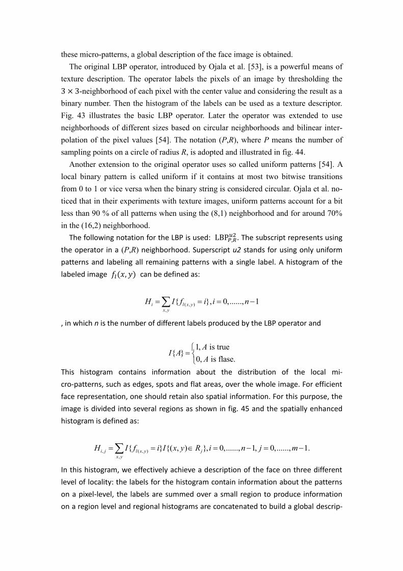
these micro-patterns, a global description of the face image is obtained.

The original LBP operator, introduced by Ojala et al. [53], is a powerful means of

texture description. The operator labels the pixels of an image by thresholding the

-neighborhood of each pixel with the center value and considering the result as a

binary number. Then the histogram of the labels can be used as a texture descriptor.

Fig. 43 illustrates the basic LBP operator. Later the operator was extended to use

neighborhoods of different sizes based on circular neighborhoods and bilinear inter-

polation of the pixel values [54]. The notation (P,R), where P means the number of

sampling points on a circle of radius R, is adopted and illustrated in fig. 44.

Another extension to the original operator uses so called uniform patterns [54]. A

local binary pattern is called uniform if it contains at most two bitwise transitions

from 0 to 1 or vice versa when the binary string is considered circular. Ojala et al. no-

ticed that in their experiments with texture images, uniform patterns account for a bit

less than 90 % of all patterns when using the (8,1) neighborhood and for around 70%

in the (16,2) neighborhood.

The following notation for the LBP is used: . The subscript represents using

the operator in a (P,R) neighborhood. Superscript u2 stands for using only uniform

patterns and labeling all remaining patterns with a single label. A histogram of the

labeled image can be defined as:

( , )

,

{ }, 0,......, 1i l x y

x y

H I f i i n

, in which n is the number of different labels produced by the LBP operator and

1, is true{ }

0, is flase.

AI A

A

This histogram contains information about the distribution of the local mi-

cro-patterns, such as edges, spots and flat areas, over the whole image. For efficient

face representation, one should retain also spatial information. For this purpose, the

image is divided into several regions as shown in fig. 45 and the spatially enhanced

histogram is defined as:

, ( , )

,

{ } {( , ) }, 0,......, 1, 0,......, 1.i j l x y j

x y

H I f i I x y R i n j m

In this histogram, we effectively achieve a description of the face on three different

level of locality: the labels for the histogram contain information about the patterns

on a pixel-level, the labels are summed over a small region to produce information

on a region level and regional histograms are concatenated to build a global descrip-

tion of the face.

In the face recognition phase, the nearest neighbor classifier is adopted to com-

pare the distance between the input face and the database. Several metrics could be

applied for distance calculation, such as the histogram intersection, log-likelihood

statistic, and distance, and Chi square statistic , etc. When the image

has been divided into regions, it can be expected that some of the regions contain

more useful information than others in terms of distinguishing between people. For

example, eyes seem to be an important cue in human face recognition. To take ad-

vantage of this, a weight can be set for each region based on the importance of the

information it contains. For example, the weighted statistic becomes

2

, ,2

, , ,

( )( , )

i j i j

w j

i j i j i j

S MX S M w

S M

, in which is the weight for region j and S and M denote two feature vectors to be

compared. Fig. 45 also shows the weights they applied in the experimental results.

Later on, several recent works used this feature for face recognition ,such as [55].

Figure 43: The basic LBP operator. [52]

Figure 44: The circular (8,2) neighborhood. The pixel values are bilinearly interpolated whenever the

sampling point is not in the center of a pixel. [52]

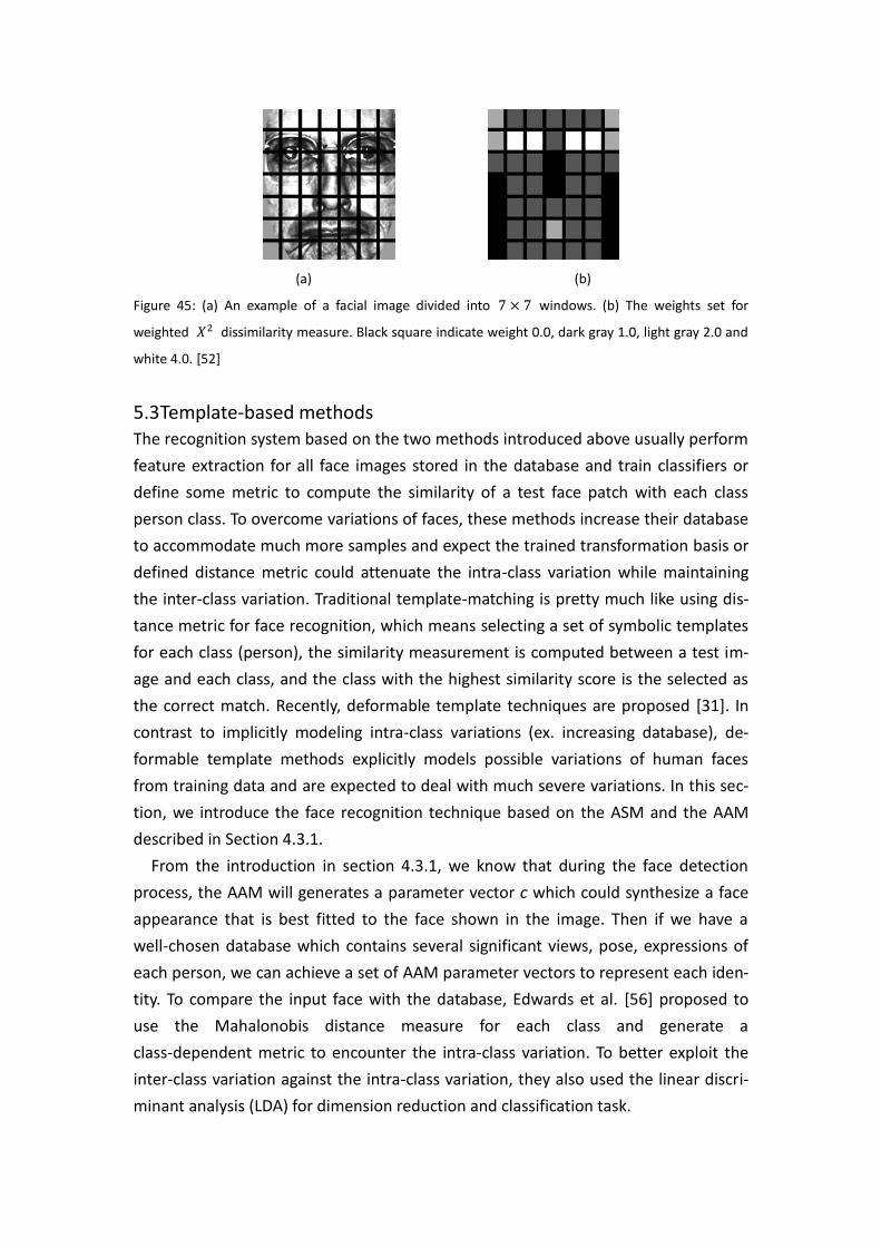
(a) (b)

Figure 45: (a) An example of a facial image divided into windows. (b) The weights set for

weighted dissimilarity measure. Black square indicate weight 0.0, dark gray 1.0, light gray 2.0 and

white 4.0. [52]

5.3 Template-based methods The recognition system based on the two methods introduced above usually perform

feature extraction for all face images stored in the database and train classifiers or

define some metric to compute the similarity of a test face patch with each class

person class. To overcome variations of faces, these methods increase their database

to accommodate much more samples and expect the trained transformation basis or

defined distance metric could attenuate the intra-class variation while maintaining

the inter-class variation. Traditional template-matching is pretty much like using dis-

tance metric for face recognition, which means selecting a set of symbolic templates

for each class (person), the similarity measurement is computed between a test im-

age and each class, and the class with the highest similarity score is the selected as

the correct match. Recently, deformable template techniques are proposed [31]. In

contrast to implicitly modeling intra-class variations (ex. increasing database), de-

formable template methods explicitly models possible variations of human faces

from training data and are expected to deal with much severe variations. In this sec-

tion, we introduce the face recognition technique based on the ASM and the AAM

described in Section 4.3.1.

From the introduction in section 4.3.1, we know that during the face detection

process, the AAM will generates a parameter vector c which could synthesize a face

appearance that is best fitted to the face shown in the image. Then if we have a

well-chosen database which contains several significant views, pose, expressions of

each person, we can achieve a set of AAM parameter vectors to represent each iden-

tity. To compare the input face with the database, Edwards et al. [56] proposed to

use the Mahalonobis distance measure for each class and generate a

class-dependent metric to encounter the intra-class variation. To better exploit the

inter-class variation against the intra-class variation, they also used the linear discri-

minant analysis (LDA) for dimension reduction and classification task.

5.4 Part-based methods Following the ideas presented in Section 4.5, there have been several researches

these years exploiting information from facial characteristic parts or parts that are

robust against pose or illumination variation for face recognition. To be distinguished

from the feature-based category, the part-based methods detect significant parts

from the face image and combine the part appearances with machine learning tools

for recognition, while the feature-based methods extract features from facial feature

points or the whole face and compare these features to achieve the recognition

purpose. In this subsection, we introduced two techniques, one is an extension sys-

tem of the method described in Section 4.5.2, and one is based on the SIFT

(scale-invariant feature transform) features extracted from the face image.

5.4.1 Component-based face recognition

Based on the face detection algorithm described in Section 4.5.2, Heisele et al. [57]

compared the performance of the component-based face recognition against the

global approaches. In their work, they generated three different face recognition

structures based on the SVM classifier: a component-based algorithm based on the

output of the component-based face detection algorithm, a global algorithm directly

fed by the detected face appearance, and finally a global approach which takes the

view variation into account.

Given the detected face patches, the two global approaches have the only differ-

ence that whether the view variation of the detected face is considered. The algo-

rithm without this consideration directly builds a SVM classifier for a person based

on all possible views, while the one with this consideration first divides the training

images of a person into several view-specific clusters, and then trains one SVM clus-

ter for each of them. The SVM classifier is originally developed for binary classifica-

tion case, and to extend for multi-class tasks, the one-versus-all and the pair-wise

approaches are described in [58]. The view-specific clustering procedure is depicted

in fig. 46.

The component-based SVM classifier is cascaded behind the component-based

face detection algorithm. After a face is detected in the image, they choose 10 of the

14 detected parts, normalized them in size and combined their gray values into a sin-

gle feature vector. Then a one-versus-all multi-class structure with a linear SVM for

each person is trained for face recognition purpose. In fig. 47, we show the face de-

tection procedure, and in fig. 48, we present the detected face and the correspond-

ing 10 components fed into the face recognition algorithm.

In the experimental results, the component system outperforms the global sys-

tems for recognition rate larger than 60% because the information fed into the clas-

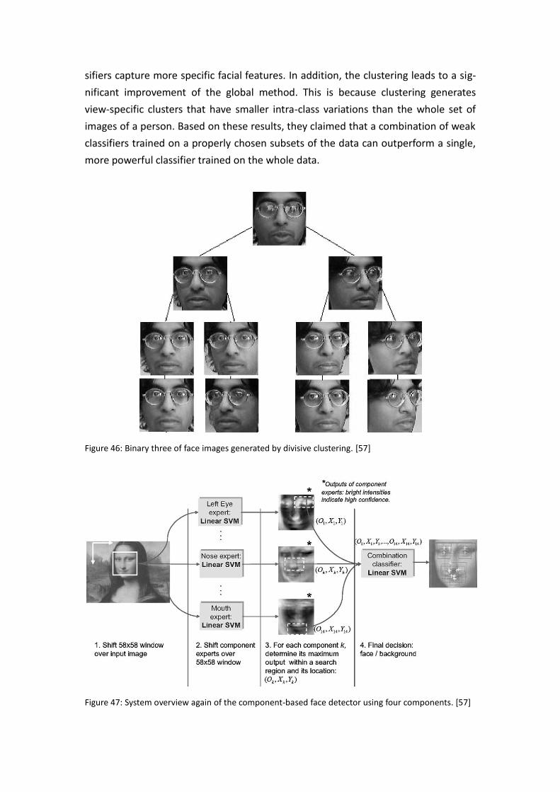
sifiers capture more specific facial features. In addition, the clustering leads to a sig-

nificant improvement of the global method. This is because clustering generates

view-specific clusters that have smaller intra-class variations than the whole set of

images of a person. Based on these results, they claimed that a combination of weak

classifiers trained on a properly chosen subsets of the data can outperform a single,

more powerful classifier trained on the whole data.

Figure 46: Binary three of face images generated by divisive clustering. [57]

Figure 47: System overview again of the component-based face detector using four components. [57]

Figure 48: Examples of the component-based face detection and the 10 components used for face

recognition. [57]

5.4.2 Person-specific SIFT features for face recognition

The scale-invariant feature transform (SIFT) proposed by Lowe et.al [34] has been

widely and successfully applied to object detection and recognition. In the works of

Luo et al. [59], they proposed to use the person-specific SIFT features and a simple

non-statistical matching strategy combined with local and global similarity on

key-point clusters to solve face recognition problems.

The SIFT is composed of two functions, the interest-point detector and the re-

gion-descriptor. Lowe et al. used the difference-of-Gaussian (DOG) algorithm to

detect these points in a scale-invariant fashion, and generated the descriptor based

on the orientation and gradient information calculated in a scale-specific region

around each detected point. Fig. 49 shows the SIFT features extracted on sample

faces and some corresponding matching point in two face images. In each face image

the number and the positions of the features selected by the SIFT point detector are

different, so these features are person-specific. In order to only compare the feature

pairs with similar physical meaning between faces in the database and the input face,

same number of sub-regions are constructed in each face image to compute the si-

milarity between each pair of sub-regions based on the features inside and at last get

the average similarity values. They proposed to ensemble a K-means clustering

scheme to construct the sub-regions automatically based on the locations of features

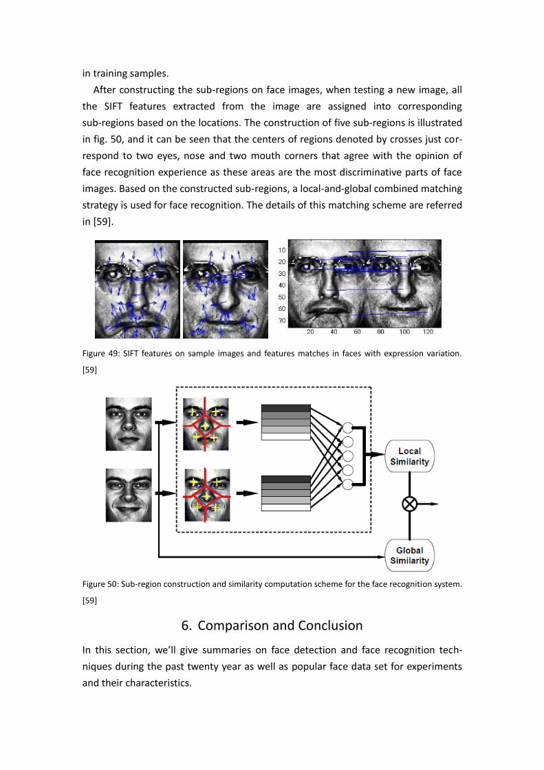
in training samples.

After constructing the sub-regions on face images, when testing a new image, all

the SIFT features extracted from the image are assigned into corresponding

sub-regions based on the locations. The construction of five sub-regions is illustrated

in fig. 50, and it can be seen that the centers of regions denoted by crosses just cor-

respond to two eyes, nose and two mouth corners that agree with the opinion of

face recognition experience as these areas are the most discriminative parts of face

images. Based on the constructed sub-regions, a local-and-global combined matching

strategy is used for face recognition. The details of this matching scheme are referred

in [59].

Figure 49: SIFT features on sample images and features matches in faces with expression variation.

[59]

Figure 50: Sub-region construction and similarity computation scheme for the face recognition system.

[59]

6. Comparison and Conclusion

In this section, we’ll give summaries on face detection and face recognition tech-

niques during the past twenty year as well as popular face data set for experiments

and their characteristics.

Table 7: The summary of face detection techniques

Method Category Characteristics

Hierarchical knowledge-based [8] Knowledge-based Coarse-to-fine procedure

Horizontal / vertical projection [9] Knowledge-based

Face Detection Using Color Information [10] Feature-based Combining skin-color detection, face shape verification, and

facial feature configuration for detection

Face detection based on random labeled

graph matching [11]

Feature-based Combining simple features with statistical learning and esti-

mation

Active appearance model [19] Template matching Learning facial shape and appearance variation by data

Example-based learning [21] Appearance-based Learning the face and non-face distribution by mixture of

Gaussian

Haar features with Adaboost [22] Appearance-based Adaboost for speed-up

Generative models [36] Part-based Unsupervisedly extracting important facial features, and

learning the relation among parts and discrimination be-

tween face and non-face by the graphical model structure.

Component-based with SVM [37] Part-based Learning global and local SVM for detection

Table 8: The summary of face recognition techniques

Method Category Characteristics

PCA [39] Holistic-based PCA for learning eigenfaces, unsupervised

LDA [40] Holistic-based LDA for learning fisherfaces, supervised

2D-PCA [41] Holistic-based 2D-PCA for better statistical properties

ICA [44] Holistic-based ICA for catch facial independent components, two archi-

tectures are proposed

Laplacianfaces [45] Holistic-based Nonlinear dimension reduction for finding bases, LPP

Evolutionary pursuit [43] Holistic-based Using the genetic algorithm for finding the best projection

bases based on generalization error

Kernel PCA And Kernel LDA [42] Holistic-based Mapping the image into higher-dimensional space by the

kernel function, and exploit the PCA and LDA bases there

Sparse representation [48] Holistic-based Using L1 minimization and over-complete dictionary for

finding sparse representation

Gabor and dynamic link architecture [49] Feature-based Gabor features extracted at facial feature locations, while

performing one-by-one matching

Gabor and elastic bunch graph matching [50] Feature-based Gabor features extracted at facial feature locations, and

obtaining the robust representation by the FBG matching.

LBP [52] Feature-based Local binary patterns are introduced

LTP [55] Feature-based Binary into ternary

AAM [56] Template matching AAM parameters for classification learning

Component-base [57] Part-based Comparing global and component representation, while a

SVM classifier for each person is not suitable in practice.

SIFT [59] Part-based Using SIFT feature with spatial constraints to compare faces

Table 9: The summary of popular databases used for detection and recognition tasks (from [3])

Name RGB/gray Image size # people Pictures/person Conditions Available

AR Face Database* RGB 576x768 126 26 i, e, o, t Yes

Richard’s MIT RGB 480x640 154 6 p, o Yes

CVL RGB 640x480 114 7 p, e Yes

The Yale Face Database B* Gray 640x480 10 576 p, i Yes

The Yale Face Database* Gray 320x243 15 11 i, e Yes

PIE* RGB 640x486 68 ~608 p ,i, e Yes

The UMIST Face Database Gray 220x220 20 19-36 p Yes

Olivetti Att-ORL* Gray 92x112 40 10 Yes

JAFFE Gray 256x256 10 7 e Yes

The Human Scan Gray 384x286 23 ~66 Yes

XM2VTSDB RGB 576x720 295 p With pay

FERET* RGB/gray 256x384 30000 p, i, e, i/o, t Yes

The (*) points out most used databases. Image variations are indicated by (i) illumination, (p) pose, (e) expression, (o) occlusion, (i/o)

indoor/outdoor conditions and (t) time delay.

Finally, there is still no robust face detection and recognition technique for uncon-

straint real-world applications, and these are our direction for future works.

Reference

[1] R. Chellappa, C. L. Wilson, and S. Sirohey, “Human and machine recognition of faces: a survey,” Proc.

IEEE, vol. 83, no. 5, pp. 705-740, 1995.

[2] W. Zhao, R. Chellappa, P. J. Phillips, and A. Rosenfeld, “Face recognition: a literature survey,” Tech-

nical Report CAR-TR-948, Center for Automation Research, University of Maryland (2002).

[3] A. F. Abate, M. Nappi, D. Riccio, and G. Sabatino, “2D and 3D face recognition: a survey,” Pattern

Recognition Letter, vol. 28, no. 14, pp. 1885–1906, 2007.

[4] M. Grgic, and K, Delac, “Face recognition homepage.” [online] Available:

http://www.face-rec.org/general-info. [Accessed May. 27, 2010].

[5] A. K. Jain, R. P. W. Duin, and J. C. Mao, “Statistical pattern recognition: a review,” IEEE Trans. Pattern

Analysis and Machine Intelligence, vol. 22, no. 1, pp. 4–37, 2000.

[6] [online] Available: http://www.michaelbach.de/ot/fcs_thompson-thatcher/index.html. [Accessed

May. 27, 2010].

[7] M. H. Yang, D. J. Kriegman, and N. Ahuja, “Detecting face in images: a survey,” IEEE Trans. Pattern

Analysis and Machine Intelligence, vol. 24, pp. 34–58, 2002.

[8] G. Yang and T. S. Huang, “Human face detection in complex background,” Pattern Recognition Let-

ter, vol. 27, no. 1, pp. 53-63, 1994.

[9] C. Kotropoulos and I. Pitas, “Rule-based face detection in frontal views,” Proc. Int’l Conf. Acoustics,

Speech and Signal Processing, vol. 4, pp. 2537-2540, 1997.

[10] R. L. Hsu, M. Abdel-Mottaleb, and A. K. Jain, ”Face detection in color images,” IEEE Trans. Pattern

Analysis and Machine Intelligence, vol. 24, no. 5, 696–706, 2002.

[11] T. K. Leung, M. C. Burl, and P. Perona, “Finding faces in cluttered scenes using random labeled

graph matching,” Proc. Fifth IEEE Int’l Conf. Computer Vision, pp. 637-644, 1995.

[12] E. Saber and A.M. Tekalp, “Frontal-view face detection and facial feature extraction using color,

shape and symmetry based cost functions,” Pattern Recognition Letters, vol. 17, no. 8, pp. 669-680,

1998.

[13] K. Sobottka and I. Pitas, “Face localization and feature extraction based on shape and color infor-

mation,” Proc. IEEE Int’l Conf. Image Processing, pp. 483-486, 1996.

[14] C. Lin, K.C. Fan, “Human face detection using geometric triangle relationship,” Proc. 15th ICPR, pp.

945–948, 2000.

[15] M. Kass, A. Witkin, and D. Terzopoulos, “Snakes: Active contour models,” Int. Journal of Computer

Vision, vol. 1, pp. 321–331, 1988.

[16] T. F. Cootes, C. J. Taylor, D. H. Cooper, and J. Graham, “Active shape models - their training and

application,” Computer Vision and Image Understanding, vol. 61, no. 1, pp. 38-59, 1995.

[17] R. O. Duda, P. E. Hart, D. G. Stoke, Pattern classification, 2nd

ed., John Wiley & Sons, 2001.

[18] T. Hastie, R. Tibshirani, and J. Friedman, The Elements of Statistical Learning, 2nd

ed., Springer,

2005.

[19] T. F. Cootes, G. J. Edwards, and C. J. Taylor, “Active appearance models,” In Burkhardt and Neu-

mann, editors, Computer Vision – ECCV’98 vol. II, 1998. Springer, Lecture Notes in Computer Science

1407, pp. 484-498, 1998.

[20] T. F. Cootes, G. J. Edwards, and C. J. Taylor, “Active appearance models,” IEEE Trans. Pattern Analy-

sis and Machine Intelligence, vol.23, no. 6, pp. 681-685, 2001.

[21] K. K. Sung and T. Poggio, “”Example-based learning for view-based human face detection,” IEEE

Trans. Pattern Analysis and Machine Intelligence, vol. 20, no.1, 39–51, 1998.

[22] P. Viola and M. Jones, “Rapid object detection using a boosted cascade of simple features,” Proc.

IEEE Conf. Computer Vision and Pattern Recognition, pp. 511 – 518, 2001.

[23] P. Viola and M. Jones, “Robust real-time face detection,” Int’l Journal of Computer Vision, vol. 57,

no. 2, pp. 137-154, 2004.

[24] H. A. Rowley, S. Baluja, and T. Kanade. “Neural network based face detection,” IEEE Trans. Pattern

Analysis and Machine Intelligence, vol. 20, no. 1, pp. 23-38, Jan. 1998.

[25] E. Osuna, R. Freund, and F. Girosi, “Training support vector machines: an application to face detec-

tion,” Proc. IEEE Conf. Computer Vision and Pattern Recognition, 1997.

[26+ E. Hjelmas and B. K. Low, “Face detection: A survey,” Computer Vision and Image Understanding,

vol. 83, pp. 236–274, 2001.

[27] P. Kakumanu, S. Makrogiannis, N. Bourbakis, "A survey of skin-color modeling and detection me-

thods," Pattern Recognition Letter, vol. 40, pp. 1106-1122, 2007.

[28] E. Alpaydin, Introduction to machine learning, 2nd

ed., The MIT Press, 2010.

[29] C. M. Bishop, Neural networks for pattern recognition, Oxford University Press, 1995.

[30] C. M. Bishop, Pattern recognition and machine learning, Springer, 2006.

[31] S. Theodoridis and K. Koutroumbas, Pattern recognition, 4th

ed., Academic Press, 2009.

[32] j, Wu, C. Brubaker, M. D. Mullin, and J. M. Rehg, “Fast asymmetric learning for cascade face detec-

tion,” IEEE Trans. Pattern Analysis and Machine Intelligence, vol. 30, no. 3, pp. 369–382, 2008.

[33] M. J. Wainwright and M. I. Jordan, ‘Graphical models, exponential families, and variational infe-

rence,” Foundations and Trends in Machine learning, vol. 1, nos. 1-2, pp. 1-305, 2008.

[34] D. G. Lowe, “Distinctive image features from scale-invariant keypoints,” Int’l Journal of Computer

Vision, vol. 60, no. 2, pp. 91-110, 2004.

[35] K. Mikolajczyk, T. Tuytelaars, C. Schmid, A. Zisserman, J. Matas, F. Schaffalitzky, T. Kadir, and L. Van

Gool, “A comparison of affine region detectors,” Int’l Journal of Computer Vision, vol. 65, pp. 43-72,

2006.

[36] R. Fergus, P. Perona, and A. Zisserman, “Object class recognition by unsupervised scale-invariant

learning,” IEEE Conf. Computer Vision and Pattern Recognition, vol. 2, pp. 264–271, 2003.

[37] B. Heisele, T. Serre, M. Pontil, and T. Poggio, “Component-based face detection,” IEEE Conf. Com-

puter Vision and Pattern Recognition, pp. 657–662, 2001.

[38] K. J. Liao, Face detection by outline, color, and facial features, Mater thesis, GICE, NTU, Taipei,

2010.

[39] M. Turk and A. Pentland, “Eigenfaces for recognition,” Journal of Cognitive Neuroscience, vol. 3,

no.1, pp. 72-86, 1991.

[40] P. N. Belhumeur, J. P. Hespanha, and D. J. Kriegman, “Eigenfaces vs. Fisherfaces: Recognition using

class specific linear projection,” IEEE Trans. Pattern Analysis and Machine Intelligence, vol. 19, no. 7,

711–720, 1997.

[41] J. Yang D. Zhang, A. F. Frangi, and J. Y. Yang, “Two-dimensional PCA: A new approach to appear-

ance-based face representation and recognition,” IEEE Trans. Pattern Analysis and Machine Intelli-

gence, vol. 26, no. 1, 131–137, 2004.

[42] M. H. Yang, ““Kernel Eigenfaces vs. Kernel Fisherfaces: Face recognition using kernel methods,”

AFGR, pp. 205–211, 2002.

[43] C. Liu and H. Wechsler, “Evolutionary pursuit and its application to face recognition,” IEEE Trans.

Pattern Analysis and Machine Intelligence, vol. 22, no. 6, pp. 570–582, 2000.

[44] M. S. Bartlett, J. R. Movellan, and T. J. Sejnowski, “Face recognition by independent component

analysis,” IEEE Trans. Neural Networks, vol. 13, no. 6, pp. 1450-1464, 2002.

[45] X. He, S. Yan, Y. Hu, P. Niyogi, and H. Zhang, “Face recognition using Laplacianfaces,” IEEE Trans.

Pattern Analysis and Machine Intelligence, vol. 27, no. 3, pp. 328-340, 2005.

[46] X. He and P. Niyogi, “Locality Preserving Projections,” Proc. Conf. Advances in Neural Information

Processing Systems, 2003.

[47] S. T. Roweis and L. K. Saul, “Nonlinear dimensionality reduction by locally linear embedding,"

Science, vol. 290, pp. 2323-2326, 2000.

[48] J. Wright, A. Y. Yang, A. Ganesh, S.S. Sastry, and Y. Ma, “Robust face recognition via sparse representation,”

IEEE Trans. Pattern Analysis and Machine Intelligence, vol. 31, no. 2, 210-227, 2009.

[49] M. Lades, J. C. Vorbriiggen, J. Buhmann, J. Lange,C. von der Malsburg, R. P. Wiirtz, and W. Konen,

“Distortion invariant object recognition in the dynamic link architecture,” IEEE Trans. on Computers,

vol. 42, no. 3, pp. 300-311, 1993.

[50] L. Wiskott, J. Fellous, N. Kruger, and C. von der Malsburg, “Face recognition by elastic bunch graph

matching,” IEEE Trans. Pattern Analysis and Machine Intelligence, vol. 19, no.7, pp. 775-779, 1997.

[51] L. Shen and L. Bai, “A review of Gabor wavelets for face recognition,” Patt. Anal. Appl., vol. 9, pp.

273-292, 2006.

*52+ T. Ahonen, A. Hadid, and M.Pietik¨ainen, “Face recognition with local binary patterns,” Proc.

Eighth European Conf. Computer Vision, pp. 469-481, 2004.

[53] T. Ojala , M. Pietikainen, D. Harwood, “A comparative study of texture measures with classification

based on feature distributions,” Pattern Recognition, vol. 29, pp. 51–59, 1996.

[54] T. Ojala , M. Pietikainen, T. Maenpaa, “Multiresolution gray-scale and rotation invariant texture

classification with local binary patterns,” IEEE Trans. on Pattern Analysis and Machine Intelligence,

vol. 24, pp. 971–987, 2002.

[55] X. Tan and B. Triggs, “Enhanced local texture feature sets for face recognition under difficult light-

ing conditions,” In: Zhou, S.K., et al. (eds.) AMFG 2007. LNCS, vol. 4778, pp. 168-182. Springer, Hei-

delberg, 2007.

[56] G.J. Edwards, T.F. Cootes, and C.J. Taylor, “Face recognition using active appearance models,” Proc.

European Conf. Computer Vision, vol. 2, pp. 581-695, 1998.

*57+ B. Heisele, P. Ho, J. Wu, and T. Poggio, “Face Recognition: Component-based versus global ap-

proaches,” Computer Vision and Image Understanding, vol. 91, nos. 1-2, pp. 6-21, 2003.

[58] R. Rifkin, Everything old is new again: a fresh look at historical approaches in machine learning,

Ph.D. thesis, M.I.T., 2002.

[59] J. Luo, Y. Ma, E. Takikawa, S. Lao, M. Kawade, and B. L. Lu, “Person-Specific SIFT Features for Face

Recognition,” Int’l Conference on Acoustic, Speech, and Signal Processing, 2007.