Fabrice Roy and Jerome Perez- Dissipationless collapse of a set of N massive particles

8/3/2019 Fabrice Roy and Jerome Perez- Dissipationless collapse of a set of N massive particles

http://slidepdf.com/reader/full/fabrice-roy-and-jerome-perez-dissipationless-collapse-of-a-set-of-n-massive 1/26

Mon. Not. R. Astron. Soc. 000, 000–000 (0000) Printed 23 September 2003 (MN LATEX style file v2.2)

Dissipationless collapse of a set of N massive particles

Fabrice Roy(1) and Jerome Perez(1,2)†(1) ´ Ecole Nationale Superieure de Techniques Avancees, Unite de Mathematiques Appliquees, 32 Bd Victor, 75015 Paris, France

(2)Laboratoire de l’Univers et de ses THeories, Observatoire de Paris-Meudon, 5 place Jules Janssen, 92350 Meudon, France

23 September 2003

ABSTRACT

The formation of self-gravitating systems is studied by simulating the collapse

of a set of N particles which are generated from several distribution functions.

We first establish that the results of such simulations depend on N for small

values of N. We complete a previous work by Aguilar & Merritt concerning

the morphological segregation between spherical and elliptical equilibria. We

find and interpret two new segregations: one concerns the equilibrium core

size and the other the equilibrium temperature. All these features are used

to explain some of the global properties of self-gravitating objects: origin of

globular clusters and central black hole or shape of elliptical galaxies.

Key words: methods: numerical, N-Body simulations – galaxies: formation

– globular clusters: general.

1 INTRODUCTION

It is intuitive that the gravitational collapse of a set of N masses is directly related to the

formation of astrophysical structures like globular clusters or elliptical galaxies (the presence

of gas may complicate the pure gravitational N -body problem for spiral galaxies). From an

analytical point of view, this problem is very difficult. When N is much larger than 2, direct

approach is intractable, and since Poincare results of non analyticity, exact solutions may

be unobtainable. In the context of statistical physics, the situation is more favorable and, in

[email protected]

† [email protected]

c 0000 RAS



2 F.Roy and J.Perez

a dissipationless approximation1, leads to the Collisionless Boltzmann Equation (hereafter

denoted by CBE)

∂f ∂t

+ p. ∂f ∂ r

+ m∂ψ∂ r

. ∂f ∂ p

= 0 (1)

where f = f (r, p, t) and ψ = ψ (r, t) are respectively the distribution function of the sys-

tem with respect to the canonically conjugated (r, p) phase space variables and the mean

field gravitational potential. As noted initially by Henon (1960), this formalism holds for

such systems if and only if we consider N identical point masses equal to m. This prob-

lem splits naturally into two related parts: the time dependent regime and the stationary

state. We can reasonably think that these two problems are not completely understood. The

transient time dependent regime was investigated mainly considering self-similar solutions

(Lynden-Bell & Eggleton (1980), Henriksen & Widrow (1995), Blottiau et al. (1988) and

Lancellotti & Kiessling (2001)). These studies conclude that power law solutions can exist

for the spatial dependence of the gravitational potential (with various powers). Nevertheless,

there is no study which indicates clearly that the time dependence of the solutions disap-

pears in a few dynamical times, giving a well defined equilibrium-like state. On the other

hand, applying Jeans theorem (e.g. Binney & Tremaine (1987) hereafter BT87, p. 220), it is

quite easy to find a stationary solution. For example, every positive and integrable function

of the mean field energy per mass unit E is a potential equilibrium distribution function

for a spherical isotropic system. Several approaches are possible to choose the equilibrium

distribution function. Thermodynamics (Violent Relaxation paradigm: Lynden-Bell (1967),

Chavanis (2002), Nakamura (2000)) indicate that isothermal spheres or polytropic systems

are good candidates. Stability analyses can be split into two categories. In the CBE context

(see Perez & Aly (1998) for a review), it is well known that spherical systems (with decreas-

ing spatial density) are generally stable except in the case where a large radial anisotropy

is present in the velocity space. This is the Radial Orbit Instability, hereafter denoted by

ROI (see Perez & Aly (1998), and Perez et al. (1998) for a detailed analytic and numeric

study of these phenomena) which leads to a bar-like equilibrium state in a few dynamical

times. In the context of thermodynamics of self-gravitating systems, in a pioneering work

1 The dissipationless hypothesis is widely accepted in the context of gravitational N -body problem because the ratio of the

two-body relaxation time over the dynamical time is of the order of N . For a system composed of more than ∼ 104 massive

particles a study during a few hundreds dynamical times can really be considered as dissipationless, the unique source of

dissipation being two-body encounters.

c 0000 RAS, MNRAS 000, 000–000



Dissipationless collapse of a set of N massive particles 3

by Antonov (1962), it was shown that an important density contrast leads to the collapse

of the core of system (see Chavanis (2003) for details).

In all these studies there is no definitive conclusion, and the choice of the equilibrium dis-

tribution remains unclear. Introducing observations and taking into account analytical con-

straints, several models are possible: chronologically, we can cite (see for example BT87, p.

223-239) the Plummer model (or other polytropic models), de Vaucouleurs r1/4 law, King

and isochrone Henon model or more recently the very simple but interesting Hernquist model

(Hernquist (1990)) for spherical isotropic systems. In the anisotropic case, Ossipkov-Merritt

or generalized polytropes can be considered. Finally for non spherical systems, there also

exists some models reviewed in BT87 (p. 245-266). Considering this wide variety of possibili-ties, one can try to make accurate numerical simulations to clarify the situation. Surprisingly,

such a program has not been completely carried on. In a pioneering work, van Albada (1982)

remarked that the dissipationless collapse of a clumpy cloud of N equal masses could lead

to a final stationary state that is quite similar to elliptical galaxies. This kind of study was

reconsidered in an important work by Aguilar & Merritt (1990), with more details and a cru-

cial remark concerning the correlation between the final shape (spherical or oblate) and the

virial ratio of the initial state. These authors explain this feature invoking ROI. Some morerecent studies (Cannizzo & Hollister (1992), Boily et al. (1999) and Theis & Spurzem (1999))

concentrate on some particularities of the preceding works. Finally, two works (Dantas et

al. (2002) and Carpintero & Muzzio (1995)) develop new ideas considering the influence of

the Hubble flow on the collapse. However, the problem is only partially depicted.

The aim of this paper is to analyse the dissipationless collapse of a large set of N Body

systems with a very wide variety of ‘realistic’ initial conditions. As we will see, the small

number of particles involved, the numerical technique or the specificity of the previous works

did not allow their authors to reach a sufficiently precise conclusion. The layout of this paper

is as follows. In section 2 we describe in detail the numerical procedures used in our experi-

ments. Section 3 describes the results we have obtained. These results are then interpreted

in section 4, where some conclusions and perspectives are also proposed.

c 0000 RAS, MNRAS 000, 000–000



4 F.Roy and J.Perez

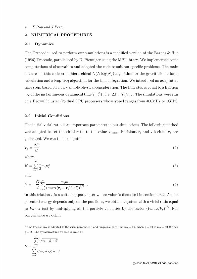
2 NUMERICAL PROCEDURES

2.1 Dynamics

The Treecode used to perform our simulations is a modified version of the Barnes & Hut

(1986) Treecode, parallelised by D. Pfenniger using the MPI library. We implemented some

computations of observables and adapted the code to suit our specific problems. The main

features of this code are a hierarchical O(N log(N )) algorithm for the gravitational force

calculation and a leap-frog algorithm for the time integration. We introduced an adaptative

time step, based on a very simple physical consideration. The time step is equal to a fraction

nts of the instantaneous dynamical time T d (2) , i.e. ∆t = T d/nts . The simulations were run

on a Beowulf cluster (25 dual CPU processors whose speed ranges from 400MHz to 1GHz).

2.2 Initial Conditions

The initial virial ratio is an important parameter in our simulations. The following method

was adopted to set the virial ratio to the value V initial. Positions ri and velocities vi are

generated. We can then compute

V p = 2K U

(2)

where

K =N

i=1

1

2miv2

i (3)

and

U = −G

2

N i= j

mim j

(max((ri − r j)2, 2))1/2. (4)

In this relation is a softening parameter whose value is discussed in section 2.3.2. As thepotential energy depends only on the positions, we obtain a system with a virial ratio equal

to V initial just by multiplying all the particle velocities by the factor (V initial/V p)1/2. For

convenience we define

2 The fraction nts is adapted to the virial parameter η and ranges roughly from nts = 300 when η = 90 to nts = 5000 when

η = 08. The dynamical time we used is given by

T d =

N

i=1 x2

i + y2i + z2

i

N i=1

vx2

i+ vy2

i+ vz2

i

c 0000 RAS, MNRAS 000, 000–000




η = |V initial| × 102 (5)

2.2.1 Homogeneous density distribution (H η)

As we study large N -body systems, we can produce a homogeneous density by generating

positions randomly. These systems are also isotropic. We produce the isotropic velocity

distribution by generating velocities randomly.

2.2.2 Clumpy density distribution (C nη )

A type of inhomogeneous systems is made of systems with a clumpy density distribution.

We first generate n small homogeneous spherical systems with radius Rg. Centers of these

subsystems are uniformly distributed in the system. The empty space is then filled using a

homogeneous density distribution. In the initial state, each clump contains about 1% of the

total mass of the system and have a radius which represents 5% of the initial radius of the

whole system. These systems are isotropic.

2.2.3 Power law r−α density distribution (P αη )

We first generate the ϕ and z cylindrical coordinates using two uniform random numbers u1

and u2:

(z, ϕ) = (2u1 − 1, 2πu2) . (6)

Using the inverse transformation method, if

r = RF −1 (u) with F (r) =1

S

r

ι

x2−αdx (7)

where R is the radius of the system, u is a uniform random number, ι 1 and

S = 1

0x2−αdx , (8)

then the probability density of r is proportional to r2−α, and the mass density ρ is propor-

tional to r−α. Finally, one gets

r =

r√

1 − z2 cos ϕ

r√

1−

z2 sin ϕ

rz

(9)

These systems are isotropic.

c 0000 RAS, MNRAS 000, 000–000



6 F.Roy and J.Perez

2.2.4 Gaussian velocity distribution(G ση )

Most of the systems we use have a uniform velocity distribution. But we have also performed

simulations with systems presenting a gaussian initial velocity distribution. These systems

are isotropic, but the x-, y- and z-components of the velocity are generated following a

gaussian distribution. Using a standard method we generate two uniform random numbers

u1 and u2, and set

vi = −2σ2 ln u1 cos(2πσ2u2) i = x,y,z (10)

where σ is the gaussian standard deviation.

2.2.5 Global rotation (Rf η )

Some of our initial systems are homogeneous systems with a global rotation around the

Z -axis. The method we choose to generate such initial conditions is the following. We create

a homogeneous and isotropic system (an H-type system). We then compute the average

velocity of the particles.

v =1

N

N

i=1

vi

(11)

We project the velocities on a spherical referential, and add a fraction of v to vφ with regard

to the position of the particle. We set

vi,φ = vi,φ + f ρiv

R(12)

where f is a parameter of the initial condition, ρi is the distance from the particle to the

Z -axis and R the radius of the system. The amount of rotation induced by this method can

be evaluated through the ratio:

µ = K rot/K, (13)

where K is the total kinetic energy defined above, whereas K rot is the rotation kinetic energy

defined by Navarro & White (1993):

K rot =1

2

N i=1

mi(Ji · Jtot)2

[r2i − (ri · Jtot)2]

(14)

Above, Ji is the specific angular momentum of particle i, Jtot is a unit vector in the direction

of the total angular momentum of the system. In order to exclude counter-rotating particles,

the sum in equation (14) is actually carried out only over those particles which verify the

condition (Ji · Jtot) > 0.

c 0000 RAS, MNRAS 000, 000–000




2.2.6 Power-law initial mass function(M kη)

Almost all the simulations we made assume particles with equal masses. However, we have

created some initial systems with a power-law mass function, like

n(M ) = αM β (15)

The number of particles whose mass is M m M + dM is n(M )dM . In some models, the

value of α and β depends on the range of mass that is considered. We have used several types

of mass functions, among them the initial mass function given by Kroupa (2001) ( k = I ),

the one given by Salpeter (1955) (k = II ) and an M −1 mass function (k = III ). In order

to generate masses following these functions, we first calculate αk to produce a continuousfunction. We then can calculate the number of particles whose mass is between M and

M + dM . We generate n(M ) masses

mi = M + udM 1 i n(M ) (16)

where 0 u 1 is a uniform random number. In the initial state, these systems have a

homogeneous number density, a quasi homogeneous mass density and they are isotropic.

2.2.7 Nomenclature

We indicate below the whole set of our non rotating initial conditions.

• Homogeneous Hη models: H88, H79, H60, H50, H40, H30, H20, H15 and H10

• Clumpy Cnη models: C20

67, C2065, C20

61, C2048, C20

39, C2029, C20

14, C2010, C20

07 and C0310

• Power Law Pαη models: P2.0

50 , P2.009 , P1.0

50 , P0.550 , P1.0

10 , P1.508 and P1.5

40

• Gaussian velocity profiles Gση models: G1

50, G250, G3

50, G412 and G5

50

• Mass spectra Mk

η models: MI

50, MII

50, MII I

51 , MI

35, MII

25, MII I

15 and MI

07

For all these models we ran the numerical simulations with 30 000 particles (see § 3.1)

2.3 Observables

2.3.1 Units

Our units are not the commonly used ones (see Heggie & Mathieu (1986)). We did not set

the total energy E of the system to−

0.25 because we wanted to prescribe instead the initial

virial ratio V initial, the size R of the system and its mass M . We thus have M = 1, R = 10

and G = 1, and values of V initial and E depending on the simulation. We can link the units

c 0000 RAS, MNRAS 000, 000–000



8 F.Roy and J.Perez

we have used with more standard ones. We have chosen the following relationships between

our units of length and mass and common astrophysical ones:

M = 106M and R = 10 pc (17)

Our unit of time ut is given by:

1ut =

R3c GsM s

R3sGcM c

≈ 4.72 1011 s = 1.50 104 yr (18)

where variables X s are expressed in our simulation units and variables X c in standard units.

2.3.2 Potential softening and energy conservation

The non conservation of the energy during the numerical evolution has three main sources.

The softening parameter ε introduced in the potential calculus (cf. equation 4) is an obvious

one. This parameter introduces a lower cutoff Λ in the resolution of length in the simulations.

Following Barnes & Hut (1989), structural details up to scale Λ 10ε are sensitive to the

value of ε. Moreover, in order to be compatible with the collisionless hypothesis, the softening

parameter must be greater than the scale where important collisions can occur. Still following

Barnes & Hut (1989), this causes

ε

10

G mv2 (19)

In our collapse simulation with 3 · 104 particles, this results in εη 2/3. The discretization

of time integration introduces inevitably another source of energy non conservation, partic-

ularly during the collapse. The force computation also generates errors. The choice of the

opening angle Θ, which governs the accuracy of the force calculation of the Treecode, is acompromise between speed and accuracy. For all these reasons, we have adopted ε = 0.1.

This choice imposes η 6 (for 30 · 104 particles). This trade-off allowed to perform simula-

tions with less than 1% energy variation without requiring too much computing time. For

each of our experiments, the total CPU time ranges between 3 to 24 hours for 3000 ut and

3 · 104 particles. The total agregated CPU time of all our collapse experiments is approxi-

mately 6 months.

We have tested two other values of the softening parameter ( ε = 0.03 and ε = 0.3) for

several typical simulations. These tests did not reveal significant variations of the computed

observables.

c 0000 RAS, MNRAS 000, 000–000




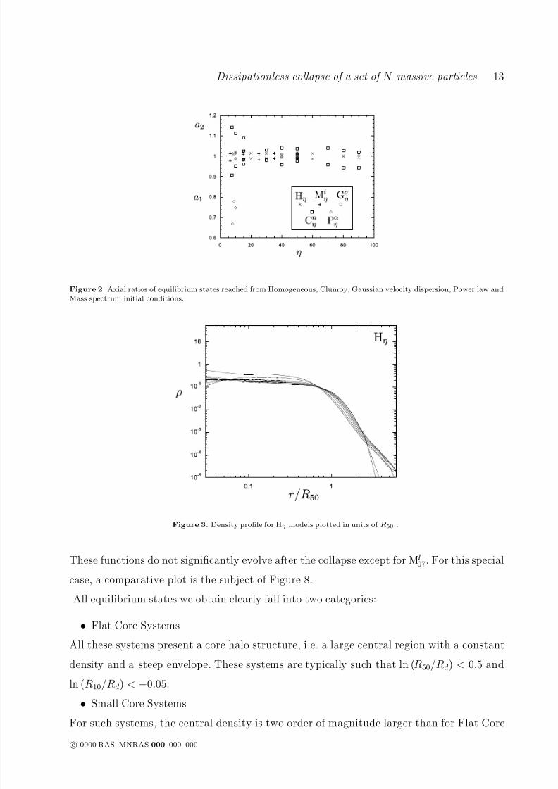
2.3.3 Spatial indicators

As indicators of the geometry of the system, we computed axial ratios, radii containing

10% (R10), 50% (R50) and 90% (R90) of the mass, density profile ρ (r) and equilibrium core

radius. The axial ratios are computed with the eigenvalues λ1, λ2 and λ3 of the (3x3) inertia

matrix I , where λ3 λ2 λ1 and, if the position of the particle i is ri = (x1,i ; x2,i ; x3,i)

I µν = − N i=1

mi xµ,i xν,i for µ = ν = 1, 2, 3

I µµ =N

i=1mi(r2

i − x2µ,i) for µ = 1, 2, 3

(20)

The axial ratios a1 and a2 are given by a2 = λ1/λ2 1.0 and a1 = λ3/λ2 1.0.The density profile ρ, which depends only on the radius r, together with the Rδ (δ =

10, 50, 90) have a physical meaning only for spherical or nearly spherical systems. For all

the spatial indicators computations we have only considered particles whose distance to the

center of mass of the system is less than 6 × R50 of the system. This assumption excludes

particles which are inevitably ‘ejected’ during the collapse3.

After the collapse a core-halo structure forms in the system. In order to measure the radius

of the core, we have computed the density radius as defined by Casertano and Hut (seeCasertano & Hut (1985)). The density radius is a good estimator of the theoretical and

observational core radius.

We have also computed the radial density of the system. The density is computed by dividing

the system into spherical bins and by calculating the total mass in each bin.

2.3.4 Statistical indicators

When the system has reached an equilibrium state, we compute the temperature of the

system

T =2 K 3N kB

(21)

where K is the kinetic energy of the system, kB is the Boltzmann constant (which is set to

1) and the notation A denotes the mean value of the observable A, defined by

A =1

N

N

i=1

Ai (22)

3 The number of excluded particles ranges from 0% to 30% of the total number of particles, depending mostly on η. For

example, the number of excluded particles is 0% for H80, 3% for C2067, 5% for H50, 22% for C20

10 and 31% for H10.

c 0000 RAS, MNRAS 000, 000–000



10 F.Roy and J.Perez

In order to characterise the system in the velocity space we have computed the function

κ (r) =2

v2

i,rad

rri<r+drv2i,tan

rri<r+dr

(23)

where vi,rad is the radial velocity of the ith particle, and vi,tan its tangential velocity. For

spherical and isotropic systems (a1 a2 1 and κ (r) 1), we have fitted the density by

1- a polytropic law

ρ = ρ0ψγ (24)

which corresponds to a distribution function

f (E ) ∝ E γ −3/2

(25)

2- an isothermal sphere law

ρ = ρ1eψ/s2

(26)

which corresponds to a distribution function

f (E ) =ρ1

(2πs2)3/2e

E

s2 (27)

Using the least square method in the ln(ρ)

−ln(ψ) plane we get (γ, ln (ρ0)) and (s2, ln (ρ1)).

3 DESCRIPTION OF THE RESULTS

We have only studied systems with an initial virial ratio corresponding to η ∈ [7, 88]. In such

systems, the initial velocity dispersion cannot balance the gravitational field. This produces

a collapse. After this collapse, in all our simulations the system reaches an equilibrium state

characterised by a temporal mean value of the virial ratio equal to −1, i.e η = 100, and

stationary physical observables. These quantities (defined in section 2) are presented in a

table of results in the appendix of this paper. The following results will be discussed and

interpreted in section 4.

3.1 Relevant number of particles

In all previous works on this subject (van Albada (1982), Aguilar & Merritt (1990), Cannizzo

& Hollister (1992) and Boily et al. (1999)), the authors did not really consider the influence

of the number of particles on their results. In the first two and more general works, this

number is rather small (not more than a few thousands in the largest simulations). The

two other studies are more specific and use typically 104 and, in a few reference cases, 2.104

c 0000 RAS, MNRAS 000, 000–000




a1

a2

N

° s2

R50

Rd

0.94

0.96

0.98

1

1.02

1.04

1

2

3

4

5

6

4

5

6

7

0.01

0.02

0.03

0.04

0.05

0.06

0 10 20 30 40 50 60 70 80

´=50

´=10

´=80

³£10

3´

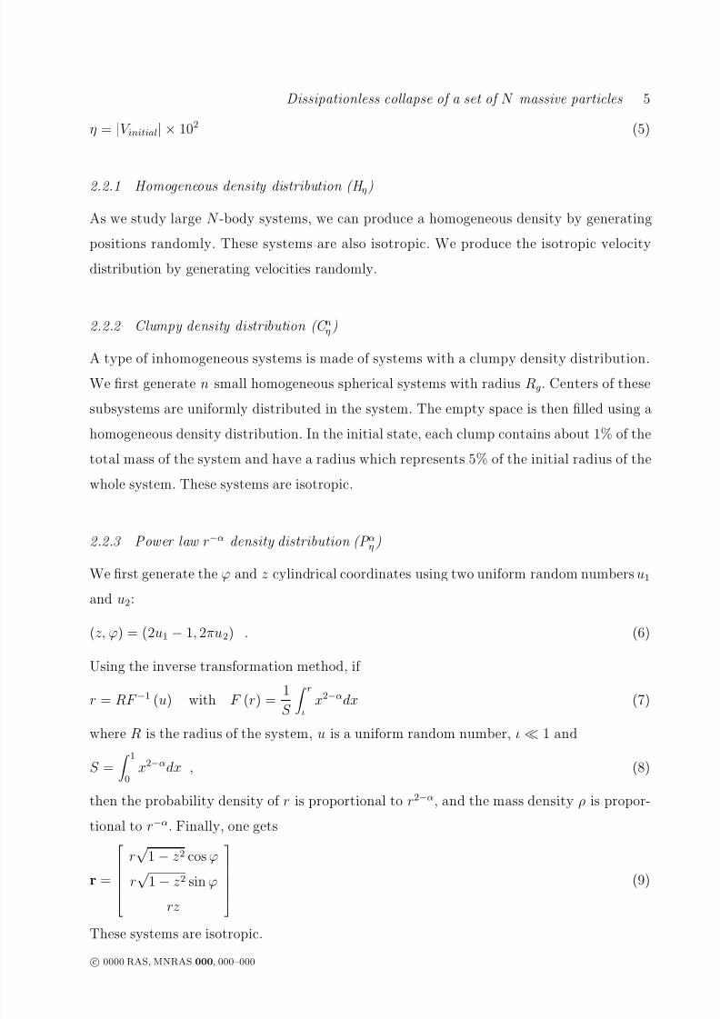
Figure 1. Influence of the number of particles on the physical observables of a collapsing system. Axial ratios are on the

top panel, radius containing 50% of the total mass and density radius are on the middle pannel and the best s2

and γ fit forrespectively isothermal and polytropic distribution function are on the bottom panel. All cases are initially homogeneous withη = 10 (solid line), η = 50 (dotted line) and η = 80 (dashed line). The number N of particles used is in units of 103.

particles. In order to test the influence of the number of particles on the final results, we

have computed several physical observables of some collapsing systems with various numbers

of particles. The results are presented in Figure 1. In order to check the influence of N in

the whole phase space, we have studied positions and velocities related observables: a1, a2,

R10, R50 and R90 and parameters of isothermal and polytropic fit models namely γ and s2.

Moreover, in order to be model-independent, we have studied three representative initial

conditions: H80, H50 and H10, i.e. respectively initially hot, warm and cold systems. The

c 0000 RAS, MNRAS 000, 000–000




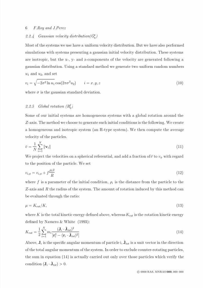
Figure 2. Axial ratios of equilibrium states reached from Homogeneous, Clumpy, Gaussian velocity dispersion, Power law andMass spectrum initial conditions.

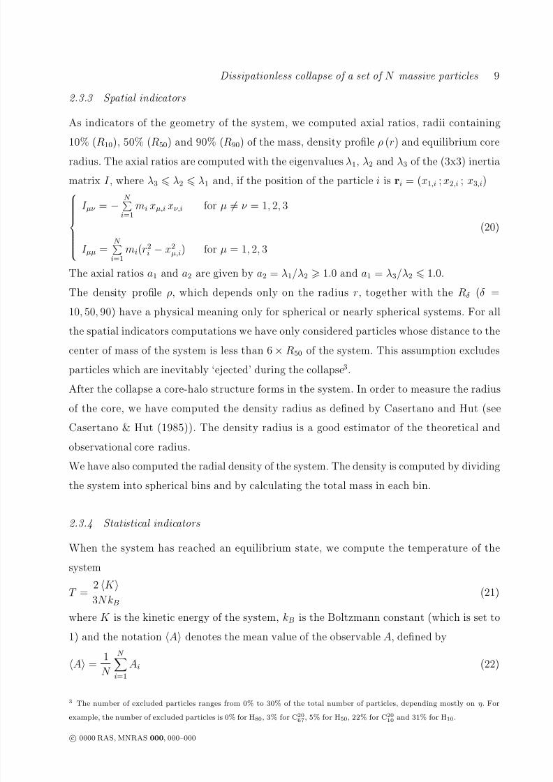
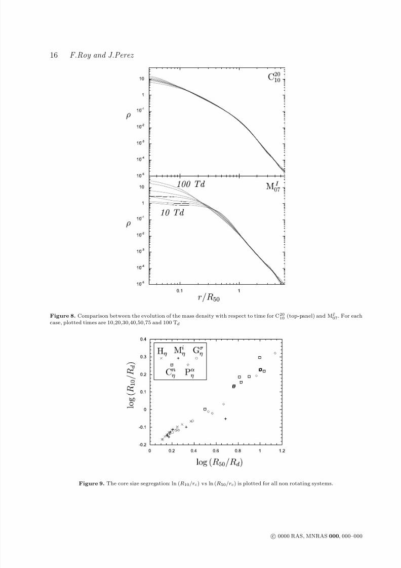
Figure 3. Density profile for Hη models plotted in units of R50 .

These functions do not significantly evolve after the collapse except for MI 07. For this special

case, a comparative plot is the subject of Figure 8.

All equilibrium states we obtain clearly fall into two categories:

• Flat Core Systems

All these systems present a core halo structure, i.e. a large central region with a constant

density and a steep envelope. These systems are typically such that ln (R50/Rd) < 0.5 and

ln (R10/Rd) <−

0.05.

• Small Core Systems

For such systems, the central density is two order of magnitude larger than for Flat Core

c 0000 RAS, MNRAS 000, 000–000




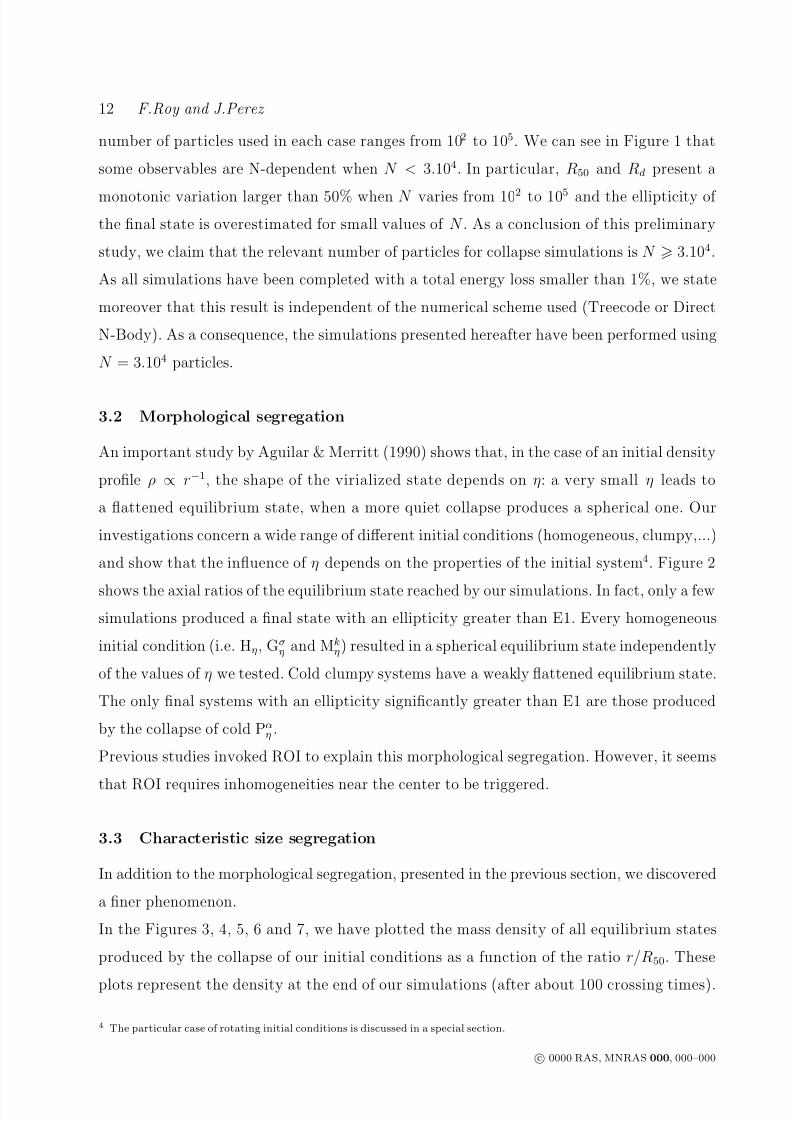
Figure 4. Density profile for Cnη models plotted in units of R50. The dashed line corresponds to the C03

10 model

Figure 5. Density profile for Pαη models plotted in units of R50.

systems. There is no central plateau and the density falls down regularly outward. These

systems are typically such that ln (R50/Rd) > 0.7 and ln (R10/Rd) > 0.1.

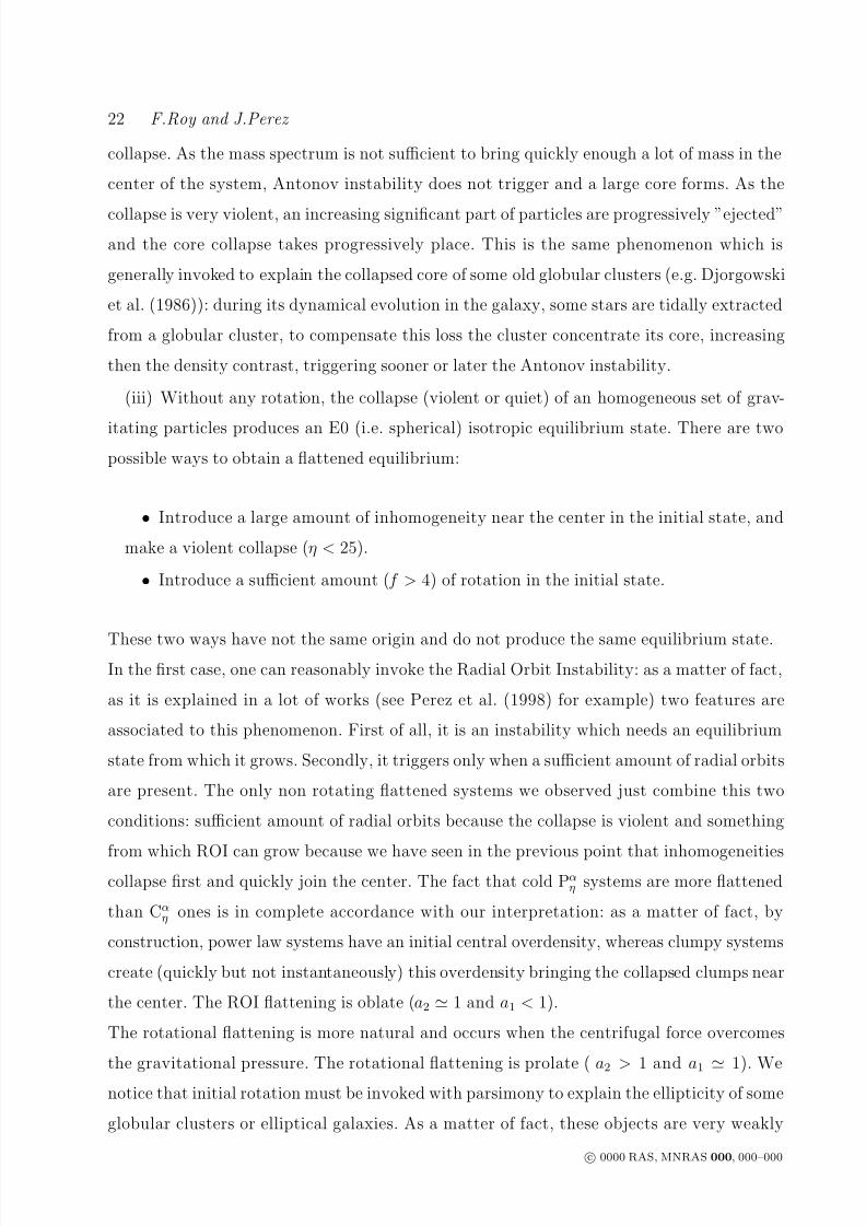
The diagram ln (R10/Rd) vs ln(R50/Rd) is the subject of Figure 9. One can see in this

figure that each equilibrium state belongs to one or the other family except in a few particular

cases. In the Flat Core family we found all Hη, Gση and Mk

η systems except MI 7, and two

Pαη systems namely P0.5

50 and P150. These systems are all initially homogeneous or slightly

inhomogeneous (e.g. P0.5

50

and P1

50

systems). In the Small Core family, we found all C20

η

and

the P2.050 and P2.0

09 systems. These systems are all initially rather very inhomogeneous. Finally,

there are 5 systems in-between the two categories: C0310, P1.5

40 , P1.508 , P1

10 and MI 07. This last

c 0000 RAS, MNRAS 000, 000–000




Figure 6. Density profile for Gση models plotted in units of R50.

Figure 7. Density profile for Mkη models plotted in units of R50.

model is the only one which migrates from Flat core set (when t 10T d) to the edge of the

small core region (when t 100T d).

3.4 Equilibrium Distribution Function

In order to compare systems in the whole phase space, we fitted the equilibrium state

reached by each system with two distinct isotropic models, e.g. polytropic and isothermal (see

equations 24-27 or BT87, p.223-232). Figure 10 shows these two fits for the P 0.5

50

simulation.

The technique used for the fit is described in section 2 of this paper. The result obtained for

this special study is the following: the equilibrium states reached by our initial conditions

c 0000 RAS, MNRAS 000, 000–000




Figure 8. Comparison between the evolution of the mass density with respect to time for C2010 (top-panel) and MI

07. For eachcase, plotted times are 10,20,30,40,50,75 and 100 Td

Figure 9. The core size segregation: ln (R10/rc) vs ln (R50/rc) is plotted for all non rotating systems.

c 0000 RAS, MNRAS 000, 000–000




Figure 10. Polytropic and isothermal fit for the P 0.550 simulation.

Figure 11. Best fit of the s2 parameter for an isothermal model for all non rotating systems studied. The error bar correspondto the least square difference between the data and the model.

can be fitted by the two models with a good level of accuracy. As long as η < 70, the

polytropic fit gives a mean value γ = 4.77 with a standard deviation of 2.48 10

−1

. Thisdeviation represents 5.1% of the mean value. This value corresponds typically to the well

known Plummer model for which γ = 5 (see BT87 P.224 for details). When the collapse

is very quiet ( typically η > 70 ) polytropic fit is always very good but the value of the

index is much larger than Plummer model, e.g. γ = 6.86 for H79 and γ = 7.37 for H88. The

corresponding plot is the subject of the Figure 12. All the data can be found in appendix.

As we can see on the example plotted in Figure 10, the isothermal fit is generally not as

good as the polytropic one. On the whole set of equilibria, isothermal fits give a mean value

s2 = 2.5 10−2 with a standard deviation of 1.6 10−2 (60%). The corresponding plot is the

subject of Figure 11. All the data can be found in appendix.

c 0000 RAS, MNRAS 000, 000–000




Figure 12. Best fit of the γ parameter for a polytropic model for all non rotating systems studied. The error bars correspondto the least square difference between the data and the model.

In fact both isothermal and polytropic fits are reasonable: as long as the model is able to

reproduce a core halo structure the fit is correct. The success of the Plummer model, which

density is given by

ρ (r) =3

4πb3

1 +r

b2−5/2

can be explained by its ability to fit a wide range of models with various ratio of the core

size over the half-mass radius. The adjustment of this ratio is made possible by varying the

free parameter b. We expect that other core halo models like King or Hernquist models work

as well as the Plummer model. As a conclusion of this section, let us say that as predicted

by theory there is not a single universal model to describe the equilibrium state of isotropic

spherical self-gravitating system.

3.5 Influence of rotation

We saw in section 3.2 a source of flattening for self-gravitating equilibrium. Let us now show

the influence of initial rotation, which is a natural candidate to produce flattening. The way

we have added a global rotation and the significance of our rotation parameters f and µ

are explained in section 2.2.5. The set of simulations performed for this study contains 31

different elements. The initial virial ratio ranges from η = 10 to η = 50, and the rotation

parameter from f = 0 (i.e. µ = 0) to f = 20 (i.e. µ = 0.16 when η = 50). As a matter of

c 0000 RAS, MNRAS 000, 000–000




Figure 13. Axial ratios as for different values of η as a function of the initial solid rotation parameter f

fact, equilibrium states always preserve a rather important part of the initial rotation5 and,

observed elliptical gravitating systems generally possess very small amount of rotation (see

e.g. Combes et al. (1995)). We thus exclude large values of f .

Our experiments exhibit two main features (see Figure 13): on the one hand, rotation

produces a flattened equilibrium state only when f exceeds a triggering value (typically

f = f o 4). On the other hand, we have found that for a given value of η, the flatness of

the equilibrium is roughly f −independent, provided that f > f o.

3.6 Thermodynamical segregation

As we study isolated systems, the total energy E contained in the system is constant during

the considered dynamical evolution . This property remains true as long as we consider

collisionless evolutions. For gravitational systems, this means that we cannot carry out any

simulation of duration larger than a few hundred dynamical times. We have obviously taken

this constraint into account in our experiments. All systems which experience a violent re-

laxation reach an equilibrium state which is stationary in the whole phase space. Spatial

behaviour like morphological segregation produced by ROI was confirmed and further de-

tailled thanks to our study. A new size segregation was found in section 3.3. Now let us

consider another new segregation appearing in the velocity space. Each equilibrium state is

associated with a constant temperature T , calculated using equation (21). More precisely,

5 We observed that µ is always smaller in the equilibrium state than in the initial one, typically each rotating systems conserves

65% of the initial µ

c 0000 RAS, MNRAS 000, 000–000




Figure 14. Evolution of the temperature as a function of time

Figure 15. Energy-Temperature diagram

we have calculated the temporal mean value 6 of the temperatures, evaluated every one

hundred time units. As we can see in Figure 14, after the collapse and whatever the nature

of the initial system is, the temperature is a very stable parameter.

Figure 15 shows the E − T diagram of the set of all non rotating simulations. It reveals a

very interesting feature of post-collapse self-gravitating systems.

On the one hand, the set of systems with a total energy E > −0.054 can be linearly fitted

in the E − T plane. We call this set Low Branch 1 (hereafter denoted by LB1, see Figure

15). On the other hand, the set of the systems with a total energy E < −0.054 splits into

two families. The first is an exact continuation of LB1. Hence we named it Low Branch 2

6 The temporal mean value is computed from the time when the equilibrium is reached until the end of the simulation

c 0000 RAS, MNRAS 000, 000–000




(hereafter denoted by LB2). The second can also be linearly fitted, but with a much greater

slope (one order of magnitude). We label this family High Branch (hereafter denoted by

HB).

In LB1 or LB2, we find every H, G, and M systems with η > 25, every P and every C with

n > 10. In HB, we find C0310 and every H, G and M systems with η < 25. This segregation

thus affects violent collapses (cold initial data): on the one hand, when η > 25 all systems

are on LB1, on the other hand for η < 25, initially homogeneous or quasi-homogeneous (e.g.

C0310) systems reach HB when initially inhomogeneous systems stay on LB2 instead.

4 INTERPRETATIONS, CONCLUSIONS AND PERSPECTIVES

Let us now recapitulate the results we have obtained and propose an interpretation:

(i) The equilibrium state produced by the collapse of a set of N gravitating particles is

N −independent provided that N > 3.0 104.

(ii) Without any rotation, the dissipationless collapse of a set of gravitating particles can

produce two relatively distinct equilibrium states:

• If the initial set is homogeneous, the equilibrium has a large core and a steep envelope.

• If the initial set contains significant inhomogeneities (n > 10 for clumpy systems or

α > 1 for power law systems), the equilibrium state has only a small core around of which

the density falls down regularly.

The explanation of this core size segregation is clear: it is associated to the Antonov

core-collapse instability occurring when the density contrast between central and outward

region of a gravitating system is very big. As a matter of fact, if the initial set contains

inhomogeneities, these collapse much more quickly than the whole system7 and fall quickly

into the central regions. The density contrast becomes then very large and the Antonov

instability triggers producing a core collapse phenomenon. The rest of the system then

smoothly collapses around this collapsed core. If there are no inhomogeneities in the initial

set, the system collapses as a whole, central density grows slowly without reaching the

triggering value of the Antonov instability. A large core then forms. Later evolution can

also produce core collapse: this is what occurs for our MI 07 system (see Figure 8). This is

an initially homogeneous system with Kroupa mass spectrum which suffers a very strong

7 Because their Jeans length is much more smaller than the one of the whole system.

c 0000 RAS, MNRAS 000, 000–000




collapse. As the mass spectrum is not sufficient to bring quickly enough a lot of mass in the

center of the system, Antonov instability does not trigger and a large core forms. As the

collapse is very violent, an increasing significant part of particles are progressively ”ejected”

and the core collapse takes progressively place. This is the same phenomenon which is

generally invoked to explain the collapsed core of some old globular clusters (e.g. Djorgowski

et al. (1986)): during its dynamical evolution in the galaxy, some stars are tidally extracted

from a globular cluster, to compensate this loss the cluster concentrate its core, increasing

then the density contrast, triggering sooner or later the Antonov instability.

(iii) Without any rotation, the collapse (violent or quiet) of an homogeneous set of grav-

itating particles produces an E0 (i.e. spherical) isotropic equilibrium state. There are twopossible ways to obtain a flattened equilibrium:

• Introduce a large amount of inhomogeneity near the center in the initial state, and

make a violent collapse (η < 25).

• Introduce a sufficient amount (f > 4) of rotation in the initial state.

These two ways have not the same origin and do not produce the same equilibrium state.In the first case, one can reasonably invoke the Radial Orbit Instability: as a matter of fact,

as it is explained in a lot of works (see Perez et al. (1998) for example) two features are

associated to this phenomenon. First of all, it is an instability which needs an equilibrium

state from which it grows. Secondly, it triggers only when a sufficient amount of radial orbits

are present. The only non rotating flattened systems we observed just combine this two

conditions: sufficient amount of radial orbits because the collapse is violent and something

from which ROI can grow because we have seen in the previous point that inhomogeneitiescollapse first and quickly join the center. The fact that cold Pα

η systems are more flattened

than Cαη ones is in complete accordance with our interpretation: as a matter of fact, by

construction, power law systems have an initial central overdensity, whereas clumpy systems

create (quickly but not instantaneously) this overdensity bringing the collapsed clumps near

the center. The ROI flattening is oblate (a2 1 and a1 < 1).

The rotational flattening is more natural and occurs when the centrifugal force overcomes

the gravitational pressure. The rotational flattening is prolate ( a2 > 1 and a1

1). We

notice that initial rotation must be invoked with parsimony to explain the ellipticity of some

globular clusters or elliptical galaxies. As a matter of fact, these objects are very weakly

c 0000 RAS, MNRAS 000, 000–000




rotating systems and our study has shown that the amount of rotation is almost constant

during the collapse.

(iv) Spherical equilibria can be suitably fitted by both isothermal and polytropic laws

with various indexes. It suggests that any distribution function of the energy exhibiting an

adaptable core halo structure (Polytrope, Isothermal, King, Hernquist,...) can suitably fit

the equilibrium produced by the collapse of our initial conditions.

(v) There exists a temperature segregation between equilibrium states. It concerns only

initially cold systems (i.e. systems which will suffer a violent collapse): for such systems

when η decreases, the equilibrium temperature T increases much more for initially homoge-

neous systems than for initially inhomogeneous systems. On the other hand, whatever their

initial homogeneity, quiet collapses are rather all equivalent from the point of view of the

equilibrium temperature: T increases in the same way for all systems as η decreases. This

feature may be the result of the larger influence of the dynamical friction induced by the

primordial core on the rapid particles in a violent collapse.

All these properties may be directly confronted to physical data from globular clusters

(see Harris catalogue Harris (1996)) or galaxies observations.

As a matter of fact, in the standard ”bottom-up” scenario of the hierarchical growth of

structures, galaxies naturally form from very inhomogeneous medium. Our study then sug-

gests for the equilibrium state of such objects a potential flattening and a collapsed core.

This is in very good accordance with the E0 to E7 observed flatness of elliptical galaxies and

may be a good explanation for the presence of massive black hole in the center of galaxies(see Schodel et al. (2002)).

On the other hand Globular Clusters observations show that these are spherical objects

(the few low flattened clusters all possess a low amount of rotation), and that their core is

generally not collapsed (the collapsed core of almost 10% of the galactic Globular Clusters

can be explained by their dynamical evolution through the galaxy). Our study then expect

that Globular Clusters form from homogeneous media.

These conclusions can be tested using the E −

T plane. As a matter of fact, we expect that

an E − T plane build from galactic data would not present any High Branch whereas the

same plane build from Globular Clusters data would.

c 0000 RAS, MNRAS 000, 000–000




ACKNOWLEDGMENTS

We thank the referee for the relevance of his remarks and suggestions. We thank Joshua

E. Barnes, who wrote the original Treecode. We also particularly thank Daniel Pfenniger

for the use of the parallel Treecode. The simulations were done on the Beowulf cluster

at the Laboratoire de Mathematiques Appliquees from the Ecole Nationale Superieure de

Techniques Avancees.

REFERENCES

Aguilar, L., and Merritt, D., 1990, ApJ, 354, 33Antonov, V.A., Vest. Len. Univ., 7, 135, 1962 in russian translated in english in Dynamics

of star clusters, Ed. Goodman J. & Hut P. (IAU 113, Reidel 1985)

Barnes, J. and Hut, P., 1986, Nature, 324, 446

Barnes, J. and Hut, P., 1989, ApJS, 70, 389

Binney, J., and Tremaine, S., 1987, Galactic dynamics, Princeton University Press

Blottiau, P., Bouquet, S., Chieze,J.-P., 1988,A&A, 207, 24

Boily, C.M., Clarke, C.J., Murray, S.D., 1999,M.N.R.A.S., 302, 399Cannizzo,J.K., and Hollister, T.C., 1992, ApJ, 400, 58

Carpintero,D.D., Muzzio, J.C., 1995, ApJ, 440, 5

Casertano, S., Hut,P., 1985, ApJ, 298, 80

Chavanis, P.-H.,2002,Submitted to Phys. Rev. E, cond-mat/0107345

Chavanis, P.-H., A& A,401, 15, 2003

Combes, F., Boisse, P., Mazure, A., Blanchard, A., 1995, Galaxies and cosmology, Springer

VerlagDantas, C.C., Capelato, H.V., de Carvalho, R.Ribiero, A.L.B, 2002, A&A, astroph-0201247

Djorgovski, S., King, I. R., Vuosalo, C., Oren, A., Penner, H.,IAU Symp.118, Ed. J.B.

Hearnshaw, P.L. Cottrell, 1986

Harris, W.E. 1996, AJ, 112, 1487

Heggie, D.C., and Mathieu R.D., 1986, in The Use of Supercomputers in Stellar Dynamics,

ed. P. Hut & S. L. W. McMillan, Springer Verlag.

Henon, M. , 1960, An.Astro, 23, 472

Henriksen, R.N., and Widrow, L.M., 1995, M.N.R.A.S, 276, 679

Hernquist, 1990, ApJ, 356, 359

c 0000 RAS, MNRAS 000, 000–000




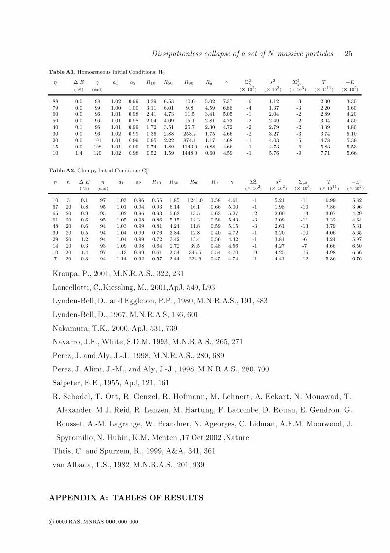
Table A1. Homogeneous Initial Conditions: Hη

η ∆ E η a1 a2 R10 R50 R90 Rd γ Σ2γ s2 Σ2

s2T −E

( %) (end) (× 102) (× 102) (× 103) (× 1011) (× 102)

88 0.0 98 1.02 0.99 3.39 6.53 10.6 5.02 7.37 -6 1.12 -3 2.30 3.3079 0.0 99 1.00 1.00 3.11 6.01 9.8 4.59 6.86 -4 1.37 -3 2.20 3.6060 0.0 96 1.01 0.98 2.41 4.73 11.5 3.41 5.05 -1 2.04 -2 2.89 4.2050 0.0 96 1.01 0.98 2.04 4.09 15.1 2.81 4.73 -2 2.49 -2 3.04 4.5040 0.1 96 1.01 0.99 1.72 3.51 25.7 2.30 4.72 -2 2.79 -2 3.39 4.8030 0.0 96 1.02 0.99 1.36 2.88 253.2 1.75 4.66 -2 3.27 -3 3.74 5.1020 0.0 101 1.01 0.99 0.95 2.22 874.1 1.17 4.68 -1 4.03 -5 4.78 5.3915 0.0 108 1.01 0.99 0.74 1.89 1143.0 0.88 4.66 -1 4.73 -6 5.83 5.5310 1.4 120 1.02 0.98 0.52 1.59 1448.0 0.60 4.59 -1 5.76 -9 7.71 5.66

Table A2. Clumpy Initial Condition: Cnη

η n ∆ E η a1 a2 R10 R50 R90 Rd γ Σ2γ s2 Σs2 T −E

( %) (end) (× 102) (× 102) (× 103) (× 1011) (× 102)

10 3 0.1 97 1.03 0.96 0.55 1.85 1241.0 0.58 4.61 -1 5.21 -11 6.99 5.8267 20 0.8 95 1.01 0.94 0.93 6.14 16.1 0.66 5.00 -1 1.98 -10 2.86 3.9665 20 0.9 95 1.02 0.96 0.93 5.63 13.5 0.63 5.27 -2 2.00 -13 3.07 4.2961 20 0.6 95 1.05 0.98 0.86 5.15 12.3 0.58 5.43 -3 2.09 -11 3.32 4.6448 20 0.6 94 1.03 0.99 0.81 4.24 11.8 0.59 5.15 -3 2.61 -13 3.79 5.3139 20 0.5 94 1.04 0.99 0.76 3.84 12.8 0.40 4.72 -1 3.20 -10 4.06 5.6529 20 1.2 94 1.04 0.99 0.72 3.42 15.4 0.56 4.42 -1 3.81 -6 4.24 5.9714 20 0.3 93 1.09 0.98 0.64 2.72 39.5 0.48 4.56 -1 4.27 -7 4.66 6.5010 20 1.4 97 1.13 0.99 0.61 2.54 345.5 0.54 4.70 -9 4.25 -15 4.98 6.667 20 0.3 94 1.14 0.92 0.57 2.44 224.6 0.45 4.74 -1 4.41 -12 5.36 6.76

Kroupa, P., 2001, M.N.R.A.S., 322, 231

Lancellotti, C.,Kiessling, M., 2001,ApJ, 549, L93Lynden-Bell, D., and Eggleton, P.P., 1980, M.N.R.A.S., 191, 483

Lynden-Bell, D., 1967, M.N.R.A.S, 136, 601

Nakamura, T.K., 2000, ApJ, 531, 739

Navarro, J.E., White, S.D.M. 1993, M.N.R.A.S., 265, 271

Perez, J. and Aly, J.-J., 1998, M.N.R.A.S., 280, 689

Perez, J. Alimi, J.-M., and Aly, J.-J., 1998, M.N.R.A.S., 280, 700

Salpeter, E.E., 1955, ApJ, 121, 161

R. Schodel, T. Ott, R. Genzel, R. Hofmann, M. Lehnert, A. Eckart, N. Mouawad, T.

Alexander, M.J. Reid, R. Lenzen, M. Hartung, F. Lacombe, D. Rouan, E. Gendron, G.

Rousset, A.-M. Lagrange, W. Brandner, N. Ageorges, C. Lidman, A.F.M. Moorwood, J.

Spyromilio, N. Hubin, K.M. Menten ,17 Oct 2002 ,Nature

Theis, C. and Spurzem, R., 1999, A&A, 341, 361

van Albada, T.S., 1982, M.N.R.A.S., 201, 939

APPENDIX A: TABLES OF RESULTS

c 0000 RAS, MNRAS 000, 000–000




Table A3. Power Law Initial Conditions: Pαη

η α ∆ E η a1 a2 R10 R50 R90 Rd γ Σ2γ s2 Σs2 T −E

( %) (end) (× 102) (× 102) (× 103) (× 1011) (× 102)

50 0.5 0.0 95 1.01 0.99 1.84 3.92 13.5 2.53 4.66 -1 2.65 -2 3.54 4.6950 1 0.0 94 1.01 0.99 1.56 3.77 12.1 2.01 4.77 -6 2.78 -3 3.69 5.0010 1 0.1 96 1.00 0.80 0.69 2.71 382.2 0.70 4.61 -8 4.05 -8 4.85 6.328 1.5 0.1 96 1.01 0.71 0.62 2.63 25.1 0.61 4.63 -7 4.42 -9 5.52 7.18

50 2 1.7 93 1.02 0.99 0.53 3.20 9.2 0.34 5.30 -6 3.35 -9 5.30 7.3240 1.5 0.1 96 1.00 0.99 0.97 3.31 11.0 1.03 4.71 -8 3.44 -6 4.42 5.999 2 1.6 96 1.01 0.78 0.38 2.51 10.6 0.18 4.68 -10 5.21 -20 6.73 9.31

Table A4. Mass Spectrum Initial Conditions: Miη

η i ∆ E η a1 a2 R10 R50 R90 Rd γ Σ2γ s2 Σs2 T −E

(% ) (end) (× 102) (× 102) (× 103) (× 1011) (× 102)

7 Krou 5.0 132 1.02 0.99 0.25 2.04 1721.0 0.37 4.26 -1 5.16 -15 9.97 5.62

15 1/M 0.6 101 1.01 0.98 0.68 2.04 366.8 0.97 4.65 -1 4.35 -10 5.72 5.5325 Salp 0.4 99 1.01 0.98 1.18 2.51 225.5 1.54 4.66 -2 3.59 -3 4.08 5.2335 Krou 0.2 98 1.01 0.99 1.55 3.18 39.8 2.09 4.66 -2 2.97 -3 3.51 4.9551 1/M 0.2 95 1.01 0.98 1.79 4.19 14.2 2.83 4.67 -9 2.39 -4 3.15 4.4850 Krou 0.1 96 1.02 0.98 1.93 4.09 15.1 2.87 4.60 -1 2.45 -3 3.19 4.5050 Salp 0.1 96 1.01 0.98 2.03 4.13 15.1 2.87 4.70 -2 2.45 -2 3.08 4.49

Table A5. Gaussian Velocity Dispersion Initial Conditions: Gση

η σ ∆ E η a1 a2 R10 R50 R90 Rd γ Σ2γ s2 Σ2

s2T −E

(% ) (end) (× 102) (× 102) (× 103) (× 1011) (× 102)

48 G1 0.0 95 1.00 1.00 1.72 3.98 14.6 2.23 4.66 -5 2.64 -3 3.13 4.5049 G2 0.0 95 1.02 0.99 1.74 4.02 14.4 2.28 4.65 -6 2.61 -3 3.13 4.50

50 G3 0.0 95 1.00 1.00 1.90 4.08 14.1 2.56 4.72 -8 2.52 -2 3.09 4.5012 G4 0.4 118 1.03 0.98 0.56 1.77 1312.0 0.64 4.56 -1 5.33 -10 6.08 5.6350 G5 0.0 96 1.01 0.99 1.98 4.11 14.8 2.72 4.71 -1 2.50 -2 3.19 4.50

Fabrice Roy and Jerome Perez- Dissipationless collapse of a set of N massive particles

Documents

Transcript of Fabrice Roy and Jerome Perez- Dissipationless collapse of a set of N massive particles