
Fabio Canova: Methods for Applied Macroeconomic...
45
COPYRIGHT NOTICE: Fabio Canova: Methods for Applied Macroeconomic Research is published by Princeton University Press and copyrighted, © 2007, by Princeton University Press. All rights reserved. No part of this book may be reproduced in any form by any electronic or mechanical means (including photocopying, recording, or information storage and retrieval) without permission in writing from the publisher, except for reading and browsing via the World Wide Web. Users are not permitted to mount this file on any network servers. Follow links for Class Use and other Permissions. For more information send email to: [email protected]
Transcript of Fabio Canova: Methods for Applied Macroeconomic...

COPYRIGHT NOTICE:
Fabio Canova: Methods for Applied Macroeconomic Research
is published by Princeton University Press and copyrighted, © 2007, by Princeton University Press. All rights reserved. No part of this book may be reproduced in any form by any electronic or mechanical means (including photocopying, recording, or information storage and retrieval) without permission in writing from the publisher, except for reading and browsing via the World Wide Web. Users are not permitted to mount this file on any network servers.
Follow links for Class Use and other Permissions. For more information send email to: [email protected]
11Bayesian Time Series and DSGE Models
This chapter covers Bayesian estimation of three popular time series models andreturns to the main goal of this book: estimation and inference in DSGE models,this time from a Bayesian perspective. All three types of time series model havea latent variable structure: the data yt depend on a latent variable xt and on avector of parameters ˛, and the latent variable xt is a function of another set ofparameters � . In factor models, xt is a common factor or a common trend; instochastic volatility models, xt is a vector of volatilities; and in Markov switchingmodels, xt is an unobservable finite-state process. While, for the first and the thirdtypes of model, classical methods to evaluate the likelihood function are available(see, for example, Sims and Sargent 1977; Hamilton 1989), for the second type,approximations based on either a method of moments or quasi-ML are typicallyused. Approximations are needed because the density of the observables f .y j ˛; �/is a mixture of distributions, that is, f .y j ˛; �/ D
Rf .y j x; ˛/f .x j �/ dx. Since
the computation of the likelihood function requires a T -dimensional integral, noanalytical solution is generally available.
As mentioned in chapter 9, the model for xt can be interpreted either as a prior oras a description of how the latent variable evolves. This means that all three modelshave a hierarchical structure which can be handled with the “data-augmentation”technique of Tanner and Wong (1987). Such a technique treatsx D .x1; : : : ; xT / as avector of parameters for which we have to compute the conditional posterior — as wehave done with the time-varying parameters of a TVC model in chapter 10. Cyclicalsampling across the conditional distributions provides, in the limit, posterior drawsfor the parameters and the unobservable x. The Markov property for xt is useful tosimplify the calculations since we can break the problem of simulating the x vectorinto the problem of simulating its components in a conditional recursive fashion.For the models we examine, the likelihood is bounded. Therefore, if the priors areproper, the transition kernel induced by the Gibbs sampler (or by the mixed Gibbs–MH sampler) is irreducible, aperiodic, and has an invariant distribution. Hence,sufficient conditions for convergence hold in these setups.
The kernel of .x; ˛; �/ is the product of the conditional distribution of .y j x; ˛/,the conditional distribution of .x j �/, and the prior for .˛; �/. Hence, g.˛; � j y/ DRg.x; ˛; � j y/ dx can be used for inference, while g.x j y/ provides a solution to
the problem of estimating x. The main difference between the setup of this chapter

11.1. Factor Models 419
and a traditional signal extraction problem is that here we produce the distributionof x at each t , not just its conditional mean. It is also important to emphasizethat, contrary to classical methods, the tools we describe allow the computation ofthe exact posterior distribution of x. Therefore, we are able to describe posterioruncertainty surrounding the latent variable and the parameters.
Forecasting ytC� and the latent variable xtC� is straightforward and can be han-dled with the tools described in chapter 9. Since many inferential exercises haveto do with the problem of obtaining a future measure of the unobserved state (thebusiness cycle in policy circles, the volatility process in business and finance cir-cles, etc.), it is important to have ways to estimate it. Draws for future xtC� can beobtained from the marginal posterior of x and the structure of its conditional.
Although this chapter primarily focuses on models with normal errors, moreheavy-tailed distributions could also be used, particularly, in finance applications.As in the case of state space models, such an extension presents few complications.
The last section of the chapter studies how to obtain posterior estimates of thestructural parameters of DSGE models, how to conduct posterior inference andmodel comparisons, and reexamines the link between DSGE models and VARs.There is very little new material in this section: we bring together the models dis-cussed in chapter 2 and the ideas contained in chapters 5–7 with the simulationtechniques presented in chapter 9 to develop a framework where structural infer-ence can be conducted in false models, taking both parameter and model uncertaintyinto consideration.
11.1 Factor Models
Factor models are used in many fields of economics and finance. They exploit theinsight that there may be a common source of fluctuations in a vector of economictime series. Factor models are therefore alternatives to the (panel) VAR modelsanalyzed in chapter 10. In the latter, detailed cross-variable interdependencies aremodeled but no common factor is explicitly considered. Here, most of interdepen-dencies are eschewed and a low-dimensional vector of unobservable variables isassumed to drive the comovements across variables. Clearly, combinations of thetwo approaches are possible (see, for example, Bernanke et al. 2005; Giannone etal. 2003). The factor structure we consider is
yit D Nyi CQiy0t C eit ;
Aei .`/eit D vit ;
Ay.`/y0t D v0t ;
9>=>; (11.1)
where E.vit ; vi 0t�� / D 0;8i ¤ i 0, i D 1; : : : ; m, E.vit ; vit�� / D �2i if � D 0
and zero otherwise, E.v0t ; v0t�� / D �20 if � D 0 and zero otherwise, and y0tis unobservable. Two features of (11.1) need to be noted. First, the unobservablefactor can have arbitrary serial correlation. Second, since the relationship betweenobservables and unobservables is static, eit is allowed to be serially correlated. y0t

420 11. Bayesian Time Series and DSGE Models
could be a scalar or a vector, as long as its dimension is smaller than the dimensionof yt . An interesting case emerges when et D .e1t ; : : : ; emt /
0 follows a VAR, i.e.,Ae.`/et D vt , and Ae.`/ is of order qe;8i .
Example 11.1. There are several specifications which fit into this framework. Forexample, y0t could be a coincident business cycle indicator which moves a vector ofmacroeconomic time series yit . In this case, eit captures idiosyncratic movementsin yit . Alternatively, y0t could be a common stochastic trend while eit is stationaryfor all i . In this latter case, (11.1) resembles the common trend-UC decompositionstudied in chapter 3. Furthermore, many of the models used in finance have a struc-ture similar to (11.1). For example, in a capital asset pricing model (CAPM), y0t isan unobservable market portfolio.
We need restrictions to identify the parameters of (11.1). Since Qi and y0t arenonobservable, neither the scale nor the sign of the factor and its loading can beseparately identified. For normalization, we choose Q1 > 0 and assume that �20 isa fixed constant.
Let ˛1i D . Nyi ;Qi /. Let ˛ D .˛1i ; �20 ; �2i ; A
ei ; A
y ; i D 1; : : : ; m/, where Aei D.Aei;1; : : : ; A
ei;qi/ andAy D .Ay1 ; : : : ; A
yq0/, be the vector of parameters of the model.
Let yi D .yi1; : : : ; yit /0 and y D .y01; : : : ; y
0m/0. Given g.˛/, g.˛ j y; y0/ /
f .y j ˛; y0/g.˛/ and g.y0 j ˛; y/ / f .y j ˛; y0/f .y0 j ˛/. To compute theseconditional distributions, we need f .y j ˛; y0/ and f .y0 j ˛/ D
Rf .y; y0 j ˛/ dy.
Consider first f .y j ˛; y0/. Let y1i D .yi;1; : : : ; yi;qi /0 be random and let
y10 D .y0;1; : : : ; y0;q0/0 be the vector of initial observations on the factors, y10
given, x1i D Œ1; y10 �, where 1 D Œ1; 1; : : : ; 1�0, and let Ai be a .qi � qi / compan-
ion matrix representation of Aei .`/. If the errors are normal, .y1i j Nyi ;Qi ; �2i ; y
10/ �
N. Nyi CQiy10 ; �
2i ˙i /, where˙i solves˙i D Ai˙iAi C .1; 0; : : : ; 0/
0.1; 0; : : : ; 0/.
Exercise 11.1. Provide a closed-form solution for ˙i .
Define y1�i D ˙�0:5i y1i and x1�i D ˙
�0:5i x1i . To build the rest of the likelihood,
let ei D Œei;qiC1; : : : ; ei;T �0 (this is .T �qi /�1 vector); eit D yit � Nyi �Qiy0t and
E D Œe1; : : : ; eqi � (this is a .T �qi /�qi matrix). Similarly, let y0 D .y01; : : : ; y0t /0
and Y0 D .y0;�1; : : : ; y0;�q0/. Let y2�i be a .T � qi / � 1 vector with the t -rowequal to Aei .`/yit and let x2�i be a .T � qi / � 2 matrix with the t -row equal to.Aei .1/; A
ei .`/y0t /. Let x�i D Œx
1�i ; x
2�i �0 and y�i D Œy
1�i ; y
2�i �.
Exercise 11.2. Derive the likelihood of .y�i j x�i ; ˛/, when et are normally dis-
tributed.
To obtaing.˛ j y; y0/, assume thatg.˛/ DQj g. j /, let �20 be fixed, and assume
that a1i � N. N1i ; N˛1i /, Aei � N. NAei ;
NAei/�.�1;1/, Ay � N. NAy ; NAy /�.�1;1/,
��2i � G.a1i ; a2i /, where �.�1;1/ is an indicator function for stationarity; that is,

11.1. Factor Models 421
the prior for Aei .Ay/ is normal, truncated outside the range .�1; 1/. Then, the con-
ditional posteriors are
.˛1i j yi ; ˛�˛1i / � N. Q˛1i .N �1˛1iN1i C �
�2i .x�i /
0y�i /;Q˛1i /;
.Aei j yi ; y0; ˛�Aei/ � N. QAe
i. N �1Ae
i
NAei C ��2i E 0iei /;
QAei/�.�1;1/ �N .Aei /;
.Ay j yi ; y0; ˛�Ay / � N. QAy . N�1AyNAy C ��20 Y 00y0/;
QAy /�.�1;1/ �N .Ay/;
.��2i j yi ; y0; ˛��i / � G..a1i C T /; a2i C .y�i � x
�i ˛1i;OLS/
2/;
9>>>>=>>>>;(11.2)
where Qai D . N �1ai C ��2i x�i
0x�i /�1, QAe
iD . N �1
Aei
C ��2i E 0iEi /�1, QAy D
. N �1Ay C ��20 Y 00Y0/
�1, while
N .Aei / D j˙Aeij�0:5 expf�.1=2�2i /.y
1i � Nyi �Qiy
10/0˙�1Ae
i.y1i � Nyi �Qiy
10/g
and
N .Ay/ D j˙Ay j�0:5 expf�.1=2�0/.y
10 � A
y.`/y10;�1/0˙�1Ay .y
10 � A
y.`/y10;�1/g:
Sampling . Nyi ;Qi ; �2i / from (11.2) is straightforward. To impose the sign restric-
tion necessary for identification, discard the draws producing Q1 6 0. The con-ditional posterior for Aei .A
y/ is complicated by the presence of the indicator forstationarity and the conditional distribution of the first qi .q0/ observations (withoutthese two, drawing these parameters would also be straightforward). Since thesedistributions are of unknown form, one could use the following variation of the MHalgorithm to draw, for example, Aei .
Algorithm 11.1.
(1) Draw .Aei /† from N. QAe
i. N �1Aei
NAei C ��2i E 0iei /;
QAei/. If
PqijD1.A
ei;j /
† > 1,discard the draw.
(2) Otherwise, draw U � U.0; 1/. If U < N ..Aei /†/=N ..Aei /
l�1/, set .Aei /l D
.Aei /†. Else set .Aei /
l D .Aei /l�1.
(3) Repeat (1) and (2) L times.
The derivation of g.y0 j ˛; y/ is straightforward. Define the T � T matrix
Q�1i D
"Qi1
Qi2
#;
where Qi1 D�˙�0:5i 0
�and
Qi2 D
26664�Aei;qi � � � �Aei;1 1 0 � � � 0
0 �Aei;qi � � � �Aei;1 1 � � � 0
� � � � � � � � � � � � � � � � � � � � �
0 0 � � � �Aei;qi � � � � � � 1
37775 ;˙i is a qi � qi matrix, and 0 is a qi � .T � qi / matrix. Similarly, define Q�10 .
422 11. Bayesian Time Series and DSGE Models
Let x†i D Q�1i xi and y†
i D Q�1i .yi � 1 Nyi /. Then the likelihood function isQmiD1 f .y
†i j Qi ; �
2i ; A
ei ; y0/, where f .y†
i j Qi ; �2i ; A
ei ; y0/ D .2��2i /
�0:5T �
expf�.y†i � QiQ
�1i y0/
0.y†i � QiQ
�1i y0/=2�
2i g. Since the marginal of the factor
is f .y0 j Ay/ D .2��20 /�0:5T expf�.Q�10 y0/
0.Q�10 y0/=2�20 g, the joint likelihood
is f .y†; y0 j ˛/ DQmiD1 f .y
†i j Qi ; �
2i ; A
ei ; y0/f .y0 j A
y/. Completing thesquares we have
g.y0 j y†i ; ˛/ � N. Qy0; Qy0/; (11.3)
where Qy0 D Qy0 ŒPmiD1 Qi�
�2i .Q�1i /0Q�1i .yi � 1 Nyi /�, Qy0 D Œ
PmiD0 Q2
i ��2i �
.Q�1i /0.Q�1i /��1 with Q0 D 1. Note that Qy0 is a T � T matrix. Given (11.2) and(11.3), the Gibbs sampler can be used to compute the joint conditional posterior of˛ and of y0, and their marginals.
To make the Gibbs sampler operative we need to select �20 and the parametersof the prior distributions. For example, �20 could be set to the average varianceof the innovations in an AR(1) regression for each yit . Since little information istypically available on the loadings and the autoregressive parameters, one could setNai1 D NA
ei D
NAy D 0 and assume a large prior variance. Finally, a relatively diffuseprior for ��2i could be chosen, for example, G.4; 0:001/, a distribution without thethird and fourth moments.
The calculation of the predictive density of y0t is straightforward and it is leftas an exercise for the reader. Note that when the factor is a common business cycleindicator, the construction of this quantity produces the density of a leading indicator.
Exercise 11.3. Describe how to construct the predictive density of y0tC� , � D1; 2; : : : .
Exercise 11.4. Suppose that i D 4 and let Aei .`/ be of first order. In addition,suppose that Ny D Œ0:5; 0:8; 0:4; 0:9�0 and Q1 D Œ1; 2; 0:4; 0:6; 0:5�0. Let Ae DdiagŒ0:8; 0:7; 0:6; 0:9�, Ay D Œ0:7;�0:3�, v0 � i.i.d. N.0; 5/, and
v � i.i.d. N
0BBB@0;266643 0 0 0
0 4 0 0
0 0 9 0
0 0 0 6
377751CCCA :
Let the priors be . Nyi ;Qi / � N.0; 10 � I2/, i D 1; 2; 3; 4, Ae � N.0; I4/�.�1;1/,Ay � N.0; I2/�.�1;1/, and ��2i � G.4; 0:001/, where �.�1;1/ instructs us to dropvalues such that
Pj A
eij > 1 or
Pj A
yj > 1. Draw sequences from the posterior of
˛ and construct an estimate of the posterior distribution of y0.
Exercise 11.5. Let the prior for . Nyi ;Qi ; Aei ; A
y ; ��2i / be noninformative. Show thatthe posterior mean of y0 is the same as the one obtained by running the Kalmanfilter/smoother on model (11.1).
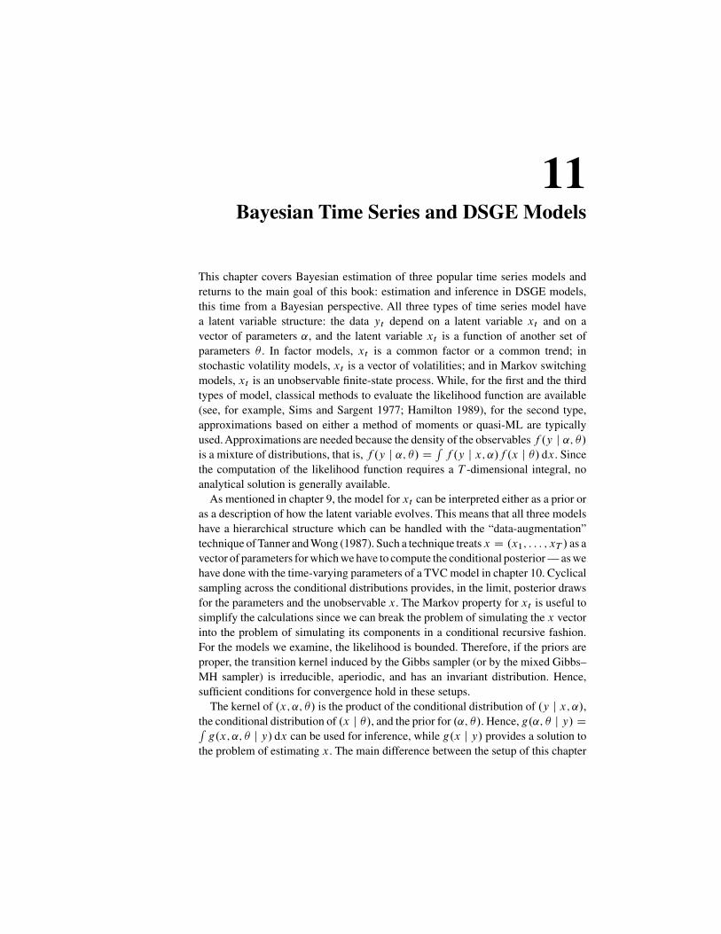
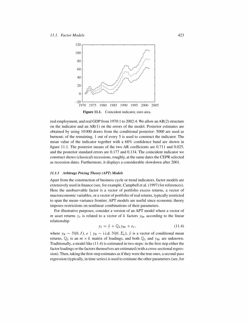
Example 11.2. We construct a coincident indicator for the euro area business cycleby using quarterly data on real government consumption, real private investment,
11.1. Factor Models 423
1970 1975 1980 1985 1990 1995 2000 2005−20
0
20
40
60
80
100
120
Figure 11.1. Coincident indicator, euro area.
real employment, and real GDP from 1970:1 to 2002:4. We allow an AR(2) structureon the indicator and an AR(1) on the errors of the model. Posterior estimates areobtained by using 10 000 draws from the conditional posterior: 5000 are used asburnout; of the remaining, 1 out of every 5 is used to construct the indicator. Themean value of the indicator together with a 68% confidence band are shown infigure 11.1. The posterior means of the two AR coefficients are 0.711 and 0.025,and the posterior standard errors are 0.177 and 0.134. The coincident indicator weconstruct shows (classical) recessions, roughly, at the same dates the CEPR selectedas recession dates. Furthermore, it displays a considerable slowdown after 2001.
11.1.1 Arbitrage Pricing Theory (APT) Models
Apart from the construction of business cycle or trend indicators, factor models areextensively used in finance (see, for example, Campbell et al. (1997) for references).Here the unobservable factor is a vector of portfolio excess returns, a vector ofmacroeconomic variables, or a vector of portfolio of real returns, typically restrictedto span the mean–variance frontier. APT models are useful since economic theoryimposes restrictions on nonlinear combinations of their parameters.
For illustrative purposes, consider a version of an APT model where a vector ofm asset returns yt is related to a vector of k factors y0t according to the linearrelationship
yt D Ny CQ1y0t C et ; (11.4)
where y0 � N.0; I /, e j y0 � i.i.d. N.0;˙e/, Ny is a vector of conditional meanreturns, Q1 is an m � k matrix of loadings, and both Q1 and y0t are unknown.Traditionally, a model like (11.4) is estimated in two steps: in the first step either thefactor loadings or the factors themselves are estimated (with a cross-sectional regres-sion). Then, taking the first-step estimates as if they were the true ones, a second-passregression (typically, in time series) is used to estimate the other parameters (see, for

424 11. Bayesian Time Series and DSGE Models
example, Roll and Ross 1980). Clearly, this approach suffers from error-in-variablesproblems and leads to incorrect inference.
A number of authors, starting from Ross (1976), have shown that, as m ! 1,absence of arbitrage opportunities implies that Nyi 0 C
PkjD1 Q1ijj , where 0
is the intercept of the pricing relationship (the so-called zero-beta rate) and j isthe risk premium on factor Q1ij , j D 1; 2; : : : ; k. With the two-step procedure wehave described, and treating the estimates of Q1ij and of Nyi as given, the restrictionsimposed become linear and tests can be easily developed by using restricted andunrestricted estimates of j (see Campbell et al. 1997).
One way to test (11.4) is to measure the pricing errors and check their sizesrelative to the average returns (with large relative errors indicating an inappropriatespecification). This measure is given by S D .1=m/ Ny0ŒI �Q.Q0Q/�1Q0� Ny, whereQ D .1;Q1/ and 1 is a vector of 1s of dimension m. For fixed m, S ¤ 0, while asm ! 1, S ! 0. While it is hard to compute the sampling distribution of S, itsexact posterior distribution can be easily obtained with MCMC methods.
For identification we require that k < 12m. Letting Qk
1 be a lower triangular matrixcontaining the Choleski transformation of the first k independent rows of Q1, wealso want Qk
1ii > 0, i D 1; : : : ; k.
Exercise 11.6. Show that k < 12m and Qk
1ii > 0, i D 1; : : : ; k, are necessary foridentification.
Let ˛i1 D . Nyi ;Qi /. Since the factors capture common components, ˙e Ddiagf�2i g. Then f .˛i1 j y0; �i / / expf�.˛i1 � ˛i1;OLS/
0x0x.˛i1 � ˛i1;OLS/=2�2i g,
where x D .1; y0/ is a T � .k C 1/ matrix and ˛i1;OLS are the OLS estimators ofthe coefficients in a regression of yit on .1; y0/. We want to compute g.˛ j y0t ; yt /and g.y0t j ˛; yt /, where ˛ D .˛1i ; �2i ; i D 1; 2; : : : /. We assume independenceacross i and the following priors: Q1i � N. NQ1i ; N�
2Q1/, Q1i i > 0, i D 1; : : : ; k,
Q1i � N. NQ1i ; N!2Q1/, i D kC 1; : : : ; m, Ns2i �
�2i � �
2. N�i /, Nyi � N. Nyi0; N�2Nyi/, where
Nyi0 D 0 CPjNQ1ijj and i are constant. The hyperparameters of all prior dis-
tributions are assumed to be known. Note that we impose the theoretical restrictionsdirectly — the prior distribution of Nyi is conditional on the value of Q1 — and that byvarying N�2yi we can account for different degrees of credence in the ATP restrictions.The conditional posterior distributions for the parameters are easily obtained.
Exercise 11.7. (i) Show that g. Nyi j yt ; y0t ;Q1; �2i / � N. QNyi ; Q�
2Nyi/, where QNyi D
Œ N�2NyiNyi;OLS C .�2i =T / Nyi0�=Œ�
2i =T C N�
2Nyi�, Q�2Nyi D Œ.�2i N�
2Nyi/=T �=Œ�2i =T C N�
2Nyi�,
Nyi;OLS D .1=T /PTtD1.yit �
PkjD1 Q1jy0tj /.
(ii) Show that g.Q1i j yt ; y0t ; Nyi ; �2i / � N. QQ1i ; QQ1i /, with QQ1i D ˙Q1i �
. NQ1i N��2Q1C x
†0i x
†iQ1i;OLS�
�2i /, QQ1i D . N�
�2Q1iC ��2i x
†0i x
†i /�1, i D 1; : : : ; k, and
QQ1i D ˙Q1i .NQ1i N!
�2Q1C x
†0i x
†iQ1i;OLS�
�2i /, QQ1i D . N!
�2Q1C ��2i x
†0i x
†i /�1, i D
k C 1; : : : ; m, where Q1i;OLS is the OLS estimator of a regression of .yit � Ny0/on y01; : : : ; y0i�1 and x†
i is the matrix xi without the first row.(iii) Show that .Qs2��2i j yt ; y0t ;Q1; Nyi / � �
2. Q�/, where Q� D N� C T and Qs2i DN� Ns2i C .T � k � 1/
Pt .yit � Nyi �
Pj Q1jy0tj /
2.
11.1. Factor Models 425
The joint density of the data and the factor is"y0t
yt
#� N
" 0
Ny
!;
I Q01
Q1 Q1Q01 C˙e
!#:
Using the properties of conditional normal distributions we have g.y0t j yt ; ˛/ �N.Q01.Q
01Q1C˙e/
�1.yt� Ny/, I�Q01.Q01Q1C˙e/
�1Q1/, with .Q01Q1C˙e/�1 D
˙�1e �˙�1e Q1.ICQ01˙
�1e Q1/
�1Q01˙�1e , where .ICQ01˙
�1e Q1/ is a k�kmatrix.
Exercise 11.8. Suppose the prior for ˛ is noninformative, that is, g.˛/ /Qj ��2j
.Derive the conditional posteriors for Ny, Q1, ˙e , and y0t in this case.
Exercise 11.9. Using monthly returns data on the stocks listed in Eurostoxx 50 forthe last five years, construct five portfolios with the quintiles of the returns. Usinginformative priors compute the posterior distribution of the pricing error in an APTmodel using one and two factors (averaging over portfolios). You may want to trytwo values for �20 , one large and one small. Report a posterior 68% credible set forS. Do you reject the theory? What can you say about the posterior mean of theproportion of idiosyncratic to total risk?
11.1.2 Conditional Capital Asset Pricing Models
A conditional CAPM combines data-based and model-based approaches to portfolioselection into a specification of the form
yitC1 D Nyit CQity0tC1 C eitC1;
Qit D x1t1i C v1it ;
Nyit D x1t2i C v2it ;
y0tC1 D x2t0 C v0tC1;
9>>>>=>>>>; (11.5)
where xt D .x1t ; x2t / is a set of observable variables, eitC1 � i.i.d. N.0; �2e /,v0tC1 � i.i.d. N.0; �20 /, and both v1it and v2it are assumed to be serially correlated,to take into account the possible misspecification of the conditioning variables x1t .Here yitC1 is the return on asset i and y0tC1 is the return on an unobservable marketportfolio. Equations (11.5) fit the factor model structure we have so far consideredwhen v2it D v1it D 0;8t , x2t are the lags of y0t and x1t D I for all t . Variousversions of (11.5) have been considered in the literature.
Example 11.3. Consider the model
yitC1 D Qit C eitC1;
Qit D xti C vit :
)(11.6)
Here the return on asset i depends on an unobservable risk premium Qit and on anidiosyncratic error term, and the risk premium is a function of observable variables.

426 11. Bayesian Time Series and DSGE Models
If we relax the assumption that the cost of risk is constant and allow time variationsin the conditional variance of asset i , we have
yitC1 D xtQt C eitC1; eit � i.i.d. N.0; �2ei /; (11.7)
Qt D QC vt ; vt � i.i.d. N.0; �2v /: (11.8)
Here the return on asset i depends on observable variables. The loadings on theobservables, assumed to be the same across assets, are allowed to vary over time.Note that by substituting the second expression into the first we have that the model’sprediction error is heteroskedastic (the variance is x0txt�
2v C �
2ei
).
Exercise 11.10. Suppose that v2it D v1it D 0;8t , and assume thaty0tC1 is known.Let ˛ D Œ21; : : : ; 2m; 11; : : : ; 1m�. Assume a priori that ˛ � N. N ; N˛/. Letthe covariance matrix of et D Œe1t ; : : : ; eMT � be ˙e and assume that, a priori,˙�1e � W. N ; N�/. Show that, conditional on .yit ; y0t ; ˙e; xt /, the posterior of ˛is normal with mean Q and variance Q˛ and that the marginal posterior of ˙�1e isWishart with scale matrix . N �1 C˙OLS/
�1 and N� C T degrees of freedom. Showthe exact form of Q , Q˛ , and ˙OLS.
Exercise 11.11. Assume v2it D v1it D 0;8t , but allow y0tC1 to be unobservable.Postulate a law of motion for y0t of the form y0tC1 D x2t0 C v0tC1, where x2tare observables. Describe the steps needed to find the conditional posterior of y0t .
The specification in (11.5) is more complicated than the one in exercises 11.10 and11.11 because of time variations in the coefficients. To highlight the steps involvedin this case, we describe a version of (11.5) where v2it D 0;8t ,m D 1, xt D x1t Dx2t , and we allow for AR(1) errors in the law of motion of Qt , that is,
ytC1 D xt2 CQty0tC1 C etC1;
Qt D .xt � xt�1/1 C Qt�1 C vt ;
y0t D xt0 C v0t ;
9>=>; (11.9)
where measures the persistence of the shock driving Qt .Let ˛ D Œ0; 1; 2; ; �
2e ; �
2v ; �
2v0� and let g.˛/ D
Qj g. j /. Assume that
g.i / � N. Ni ; N�i /, i D 0; 1; 2, g./ � N.0; N /�.�1;1/, g.��2v / � �.Ns2v ; N�v/,g.��2e ; ��2v0 / / �
�2e ��2v0 , and that all hyperparameters are known.
To construct the conditional posterior of Qt note that, if is known, Qt canbe easily simulated as in state space models. Therefore, partition ˛ D .˛1; /.Conditional on , the law of motion of Qt is y � Q � Q�1 D x
C1 C v, whereQ D ŒQ1; : : : ;Qt �
0, x D Œx1; : : : ; xt �0, xC D x � x�1, and v � i.i.d. N.0; �2v IT /.Setting QtD�1 D 0, we have two sets of equations, one for the first observation andone for the others, y0 � Q0 D xC0 1 C v0 and yt � Qt � Qt�1 D xCt 1 C vt .When the errors are normal, the likelihood function f .y j x; 1; / is proportionalto .�2v /
�0:5T expf�0:5Œ.y0 � xC0 1/�
�2v .y0 � x
C0 1/
0 �PTtD1.yt � x
Ct 1/�
�2v �
.yt � xCt 1/
0�g.

11.2. Stochastic Volatility Models 427
Let01;OLS be the OLS estimator obtained from the first observation and11;OLS theOLS estimator obtained from the other observations. Combining the prior and thelikelihood, the posterior kernel of is proportional to expf�0:5.01 �
01;OLS/
0 �
.xC0 /0��2v xC0 .
10 �
10;OLS/ � 0:5
Pt .
11 �
11;OLS/
0.xCt /0��2v xCt .
11 �
11;OLS/ �
0:5.1� N1/0 N �1�1.1� N1/g. Therefore, the conditional posterior for 1 is normal.
The mean is a weighted average of prior mean and two OLS estimators, i.e., Q1 DQ�1.N �1�1N1C.x
C0 /0��2v y0C
Pt .xCt /0��2v yt / and Q�1 D . N
�1�1C.xC0 /
0��2v xC0 CPt .xCt /0��2v xCt /
�1. The conditional posterior for�2v can be found by using the samelogic.
Exercise 11.12. Show that the posterior kernel for �2v has the form .�2v /�0:5.T�1/�
expf�0:5Pt ��2v .yt � x
Ct 1/
0.yt � xCt 1/gŒ.�
2v =.1 �
21//
0:5��0:5. N�vC1C2/ �
expf�0:5Œ�2v =.1�21/��1Œ.y0 � x
C0 1/
0.y0 � xC0 1/C N�v�g. Suggest an algorithm
to draw from this (unknown) distribution.
Once the distribution for the components of ˛1 is found, we can use the Kalmanfilter/smoother to construct Qt and the posterior of y0t , conditional on . To findthe posterior distribution of requires little more work. Conditional on 1, rewritethe law of motion for Qt as y†
t � Qt � xt1 D x†t�1C vt , where x†
t�1 D
Qt�1 � xt�11. Once again, split the data in two: initial observations .y†1; x
†0/ and
the rest .y†t ; x
†t�1/. The likelihood function is
f .y† j x†; 1; / / ��Tv expf�0:5.y†
1 � x†01/
0��2v .y†1 � x
†01/g
C exp
��0:5
Xt
.y†t � x
†t�11/
0��2v .y†t � x
†t�11/
�: (11.10)
Let OLS be the OLS estimator of obtained with T data points. Combining thelikelihood with the prior produces a kernel of the form expf�0:5
Pt . � OLS/
0 �
.x†t /0��2v x
†t . � OLS/ C . � N
0/ N �1 . � N/gŒ.�2v =.1 � 21//
0:5��0:5. N�vC1C2/ �
expf�0:5Œ�2v =.1 � 21/��1 N�v C .y
†1/0Œ�2v =.1 �
21/��1y
†1g. Hence, the conditional
posterior for is normal, truncated outside the range .�1; 1/, with mean Q DQ . N
�1 NC
Pt .x
†t /0��2v y
†t /, variance Q D . N �1 C
Pt .x
†t /0��2v x
†t /�1.
Exercise 11.13. Provide an MH algorithm to draw from the conditional posteriorof .
Once g.˛1 j ; y0t ; yt /, g. j ˛1; y0t ; yt /, g.y0t j ˛1; ; yt / are available, theGibbs sampler can be used to find the joint posterior of the quantities of interest.
11.2 Stochastic Volatility Models
Stochastic volatility models are alternatives to GARCH or TVC models. In fact,they can account for time-varying volatility and leptokurtosis as GARCH or TVCmodels but produce excess kurtosis without heteroskedasticity. Since the logarithmof �2t is assumed to follow an AR process, changes in yt are driven by shocks inthe model for the observables or shocks in the model for the logarithm of �2t . Such
428 11. Bayesian Time Series and DSGE Models
a feature adds flexibility to the specification and produces richer dynamics for theobservables as compared with, for example, GARCH-type models, where the samerandom variable drives both observables and volatilities.
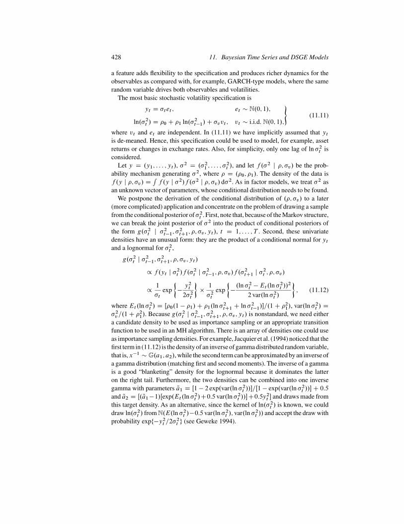
The most basic stochastic volatility specification is
yt D �tet ; et � N.0; 1/;
ln.�2t / D 0 C 1 ln.�2t�1/C �vvt ; vt � i.i.d. N.0; 1/;
)(11.11)
where vt and et are independent. In (11.11) we have implicitly assumed that ytis de-meaned. Hence, this specification could be used to model, for example, assetreturns or changes in exchange rates. Also, for simplicity, only one lag of ln �2t isconsidered.
Let y D .y1; : : : ; yt /, �2 D .�21 ; : : : ; �2t /, and let f .�2 j ; �v/ be the prob-
ability mechanism generating �2, where D .0; 1/. The density of the data isf .y j ; �v/ D
Rf .y j �2/f .�2 j ; �v/ d�2. As in factor models, we treat �2 as
an unknown vector of parameters, whose conditional distribution needs to be found.We postpone the derivation of the conditional distribution of .; �v/ to a later
(more complicated) application and concentrate on the problem of drawing a samplefrom the conditional posterior of�2t . First, note that, because of the Markov structure,we can break the joint posterior of �2 into the product of conditional posteriors ofthe form g.�2t j �
2t�1; �
2tC1; ; �v; yt /, t D 1; : : : ; T . Second, these univariate
densities have an unusual form: they are the product of a conditional normal for ytand a lognormal for �2t ,
g.�2t j �2t�1; �
2tC1; ; �v; yt /
/ f .yt j �2t /f .�
2t j �
2t�1; ; �v/f .�
2tC1 j �
2t ; ; �v/
/1
�texp
��y2t
2�2t
��1
�2texp
��.ln �2t �Et .ln �
2t //
2
2 var.ln �2t /
�; (11.12)
where Et .ln �2t / D Œ0.1 � 1/C 1.ln �2tC1 C ln �2t�1/�=.1C 21/, var.ln �2t / D
�2v =.1C 21/. Because g.�2t j �
2t�1; �
2tC1; ; �v; yt / is nonstandard, we need either
a candidate density to be used as importance sampling or an appropriate transitionfunction to be used in an MH algorithm. There is an array of densities one could useas importance sampling densities. For example, Jacquier et al. (1994) noticed that thefirst term in (11.12) is the density of an inverse of gamma distributed random variable,that is,x�1 � G.a1; a2/, while the second term can be approximated by an inverse ofa gamma distribution (matching first and second moments). The inverse of a gammais a good “blanketing” density for the lognormal because it dominates the latteron the right tail. Furthermore, the two densities can be combined into one inversegamma with parameters Qa1 D Œ1 � 2 exp.var.ln �2t //�=Œ1 � exp.var.ln �2t //�C 0:5and Qa2 D Œ. Qa1�1/Œexp.Et .ln �2t /C0:5 var.ln �2t //�C0:5y
2t � and draws made from
this target density. As an alternative, since the kernel of ln.�2t / is known, we coulddraw ln.�2t / from N.E.ln �2t /�0:5 var.ln �2t /; var.ln �2t // and accept the draw withprobability expf�y2t =2�
2t g (see Geweke 1994).

11.2. Stochastic Volatility Models 429
Table 11.1. Percentiles of the approximating distributions.
Percentiles‚ …„ ƒ5th 25th 50th 75th 95th
Gamma 0.11 0.70 1.55 3.27 5.05Normal 0.12 0.73 1.60 3.33 5.13
Example 11.4. We have run a small Monte Carlo experiment to check the qualityof these two approximations. Table 11.1 reports the percentiles using 5000 drawsfrom the posterior when 0 D 0:0, 1 D 0:8, and �v D 1:0. Both approximationsappear to produce similar results.
It is worthwhile stressing that (11.11) is a particular nonlinear Gaussian modelwhich can be transformed into a linear but non-Gaussian state space model withoutloss of information. In fact, letting xt D ln �t , �t D ln e2t C1:27; the model (11.11)could be written as
ln y2t D �1:27C xt C �t ;
xtC1 D xt C �vvt ;
)(11.13)
where �t has zero mean but is nonnormal. A framework like this was encountered inchapter 10 and techniques designed to deal with such models were outlined there.Here it is sufficient to point out that a nonnormal density for �t can be approxi-mated with a mixture of J normals, that is, f .�t /
Pj %jf .�t jMj /, where each
f .�t jMj / � N.N�j ; �2�j/ and 0 6 %j 6 1. Chib (1996) provides details on how this
can be done.Cogley and Sargent (2005) have recently applied the mechanics of stochastic
volatility models to a BVAR with time-varying coefficients. Since the setup theyuse could be employed as an alternative to the linear time-varying conditional struc-tures we studied in chapter 10, we will examine in detail how to obtain conditionalposterior estimates for the parameters of such a model.
A VAR model with stochastic volatility has the form
yt D .Im ˝Xt /˛t C et ; et � N.0;˙†t /;
˙†t D P�1˙t .P
�1/0;
˛t D D1˛t�1 C v1t ; v1t � N.0;˙v1/;
9>=>; (11.14)
where P is a lower triangular matrix with 1s on the main diagonal,˙t D diagf�2itg,
ln �2it D ln �2it�1 C �v2i v2it ; (11.15)
where D1 is such that ˛t is a stationary process. In (11.14) the process for ythas time-varying coefficients and time-varying variances. To compute conditionalposteriors note that it is convenient to block together the ˛t and the �2t and draw awhole sequence for these two vectors of random variables.

430 11. Bayesian Time Series and DSGE Models
We make standard prior assumptions, i.e., ˛0 � N. N ; Na/,˙�1v1 �W. Nv1 ; N�v1/,where Nv1 / Na, N�v1 D dim.˛0/C 1, ��2v2i � G.a1; a2/, ln �i0 � N.ln N�i ; N� /,and letting represent the nonzero elements of P , � N. N; N�/.
Given these priors, the calculation of the conditional posterior for .˛t ; ˙v1 ; �v2i /is straightforward. The conditional posterior for ˛t can be obtained with a runof the Kalman filter as detailed in chapter 10; the conditional posterior for˙�1v1 is W.. N �1v1 C
Pt v1tv
01t /�1; N�v1 C T /, and that for ��2v2i is G.a1 C T; a2 CP
t .ln �2it � ln �2it�1/
2/.
Example 11.5. Suppose yt D ˛tyt�1Cet , et � i.i.d. N.0; �2t /, ˛t D ˛t�1Cv1t ,v1t � i.i.d. N.0; �2v1/, ln �2t D ln �2t�1 C �v2v2t , v2t � i.i.d. N.0; 1/. If ��2v2 �G.av2 ; bv2/ and ��2v1 � G.av1 ; bv1/, then, given , the conditional posteriors of.��2v1 ; �
�2v2/ are gamma with parameters .av1 C T; bv1 C
Pt v21t / and .av2 C T ;
Nbv2 CPt .ln �
2t � ln �2t�1/
2/, respectively.
Exercise 11.14. Derive the conditional posteriors of .; ��2v1 ; ��2v2/ in example 11.5
when is unknown and has prior N. N; N�2 /�.�1;1/, where �.�1;1/ is an indicator forstationarity.
To construct the conditional of , note that, if �t � .0;˙t /, then et D P �t �.0;P˙tP
0/. Hence, if et is known, and given .yt ; xt ; ˛t /, the free elements of Pcan be estimated as follows. Since P is lower triangular, the mth equation is
��1mt emt D m1.���1mt e1t /C � � � C m;m�1.��
�1mt em�1t /C .�
�1mt �mt /: (11.16)
Hence, letting Emt D .���1mt e1t ; : : : ;���1mt�1emt /, "mt D ��
�1mt �mt , it is easy to
see that the conditional posterior for i is normal with mean Qi and variance Q�i .
Exercise 11.15. Show the form of Qi and Q�i .
To draw �2it from its conditional distribution, let �2.�i/t
be the sequence of �2texcluding its i th element and let e D .e1; : : : ; et /. Then g.�2it j �
2.�i/t
; ��i ; e/ D
g.�2it j �2it�1; �
2itC1; ��i ; e/, which is given in (11.12). To draw from this distri-
bution for each i we could choose as candidate distribution ��2it expf�.ln �2it �Et .ln �2it //
2=2 var.ln �2t /g and accept or reject the draw with probability .�†it /�1 �
expf�e2it=2.�2it /
†g=.�`�1it /�1 expf�e2it=2.�2it /l�1g, where .�2it /
l�1 is the last drawand .�2it /
† is the candidate draw.
Exercise 11.16. Suppose you are interested in predicting future values of yt . LetytC� D .ytC1; : : : ; ytC� /, ˛ D .˛1; : : : ; ˛t /, and y D .y1; : : : ; yt /. Show that,conditional on time t information,
g.ytC� j ˛;˙†t ; ˙v1 ; ; �v2i ; y/
D
“g.˛tC� j ˛;˙
†t ; ˙v1 ; ; �v2i ; y/
� g.˙†;tC� j ˛tC� ; ˙†t ; ˙v1 ; ; �v2i ; y/
� f .ytC� j ˛tC� ; ˙†;tC� ; ˙v1 ; ; �v2i ; y/ d˛tC� d˙†;tC� :
11.2. Stochastic Volatility Models 431
Describe how to sample .ytC1; ytC2/ from this distribution. How would you con-struct a 68% prediction band?
Stochastic volatility models are typically used to infer values for the unobservableconditional volatilities, both in-sample (smoothing) and out-of-sample (prediction).For example, option pricing formulas require estimates of conditional volatilitiesand event studies often relate specific occurrences to changes in volatility. Here weconcentrate on the smoothing problem, that is, on the computation of g.�2t j y/,where y D .y1; : : : ; yT /. An analytic expression for this posterior density is notavailable but since g.�2t j y/ D
Rg.�2t ; j ˛t ; y/g.˛t j y/ d˛t it can be numerically
obtained by using the draws of �2t and ˛t . The mean of this distribution can be usedas an estimate of the smoothed volatility.
Exercise 11.17. Suppose the volatility model is ln �2t D 0C .`/ ln �2t�1C �vvt ,where .`/ is unknown of order q. Show how to extend the Gibbs sampler to thiscase. Assume now that the model is of the form ln �2t D 0 C 1 ln �2t�1 C �vt vt ,where �vt D f .xt /,xt are observable variables, andf is linear. Show how to extendthe Gibbs sampler to this case.
As with factor models, cycling through the conditionals of .˙†t ; ˛t ; �v2i ; ˙v1 ; /
with the Gibbs sampler produces, in the limit, a sample from the joint posterior.Uhlig (1994) proposed an alternative specification for a stochastic volatility model
which, together with a particular distribution of the innovations of the stochasticvolatility term, produces closed-form solutions for the posterior distribution of theparameters and of the unknown vector of volatilities. The approach treats someparameters in the stochastic volatility equation as fixed but has the advantage ofproducing recursive estimates of the quantities of interest.
Consider an m-variable VAR(q) with stochastic volatility of the form
Yt D AXt CP�1t et ; et � N.0; I /;
˙tC1 DP 0tvtPt
; vt � Beta..� C k/=2; 1=2/;
9>=>; (11.17)
where Xt contains the lags of the endogenous and the exogenous variables, Pt isthe upper Choleski factor of ˙tC1, � and are (known) parameters, Beta denotesthem-variate beta distribution, and k is the number of parameters in each equation.
To construct the posterior of the parameters of (11.17) we need a prior for .A;˙1/.We assume g1.A;˙1/ / g0.A/g.A;˙1 j NA0; NA; N0; N�/, where g0.A/ is a func-tion restricting the prior forA (e.g., to be stationary) and g.˛;˙1 j NA0; NA; N0; N�/is of normal-Wishart form, i.e., g.A j ˙1/ � N. NA0; NA/, g.˙�11 / � W. N0; N�/,NA0, N0, NA, N�, known.
Combining the likelihood of (11.17) with these priors and exploiting the fact thatthe beta distribution conjugates with the gamma distribution, we have that the pos-terior kernel for .A;˙tC1/ is Jgt .A;˙tC1/ D Jgt .A/ Jg.A;˙tC1 j QAt ; QAt ; Q t ; �/,

432 11. Bayesian Time Series and DSGE Models
where Jg is of normal-Wishart type, QAt D QAt�1 CXtX 0t , QAt D . QAt�1 QAt�1CYtX
0t /Q �1At , Q t D Q t�1 C .=�/et .1 �X 0t Q
�1At Xt / Qe
0t , Qet D Yt � QAt�1Xt , and
Jgt .A/ D Jgt�1.A/j.A � QAt / QAt .A � QAt /0 C .�=/ Q t j
�0:5.
Example 11.6. Consider a univariate AR(1) version of (11.17) of the form
yt D ˛yt�1 C ��1t et ; et � N.0; 1/; (11.18)
�2tC1 D �2t vt ; vt � Beta..� C 1/=2; 1=2/: (11.19)
Let g.˛; �21 / / g0.˛/g.˛; �21 j N0; N�
2˛0; N�20 ; N�/, where . N0; �˛0 ; N�0; N�/ are hyper-
parameters and assume that g.˛; �21 j N0; N�2˛0; N�20 ; N�/ is of normal-inverted gamma
type. Recursive posterior estimates of the parameters of gt .˛/ are Q�2˛;t D Q�2˛;t�1C
y2t�1, Q t D . Q t�1�2˛;t�1Cytyt�1/=�2˛;t , Q�
2t D Q�
2t�1C .=�/ Qe
2t .1�y
2t�1=�
2˛;t /,
Qet D yt � Q t�1yt�1, gt .˛/ D gt�1.˛/Œ.˛ � Q t /2�2˛;t C .�=/�2t ��0:5. Hence both
Q�2˛t and Q are weighted averages, with measuring the memory of the process.Note that past values of Q are weighted by the relative change in Q�2˛;t . When �2˛;t isconstant, Q t D Q t�1 C ytyt�1=�2˛ .
When D �=.� C 1/, �= D 1 � . In this case, Q�2t is a weighted average ofQ�2t�1 and the information contained in the square of the recursive residuals, adjustedfor the relative size of y2t , to the weighted sum of y2t�1 up to t � 1. Note also thatEt�1�
2t D �2t�1.� C 1/=.� C 2/. Hence, when D .� C 1/=.� C 2/, �2t is a
random walk.
For comparison, it may be useful to map the general prior of (11.17) into aMinnesota-type prior. For example, we could set N0 D diagf N�0ig and compute N�0ifrom the average square residuals of an AR(1) regression for each i in a trainingsample. Also, one could set NA D blockdiagŒ NA1; NA2�, where the split reflectsthe distinction between endogenous and exogenous variables. For example, if thesecond block contains a constant and linear trend, then
NA2 D
"2 �22=2
22=2 �32=3
#;
where 2 is a hyperparameter, while we could set the diagonal elements of ˙A1equal to �20 �
21 =`, where ` refers to the lag, and 1 for the lags of the variables in
an equation, and the off-diagonal elements to zero. Unless required by the problem,set g0.A/ D 1. Finally, set � 20 for quarterly data and D �=.� C 1/.
Given the generic structure for the posterior of .At ; ˙tC1/ (a time-varying den-sity multiplied by a normal-Wishart density), we need numerical methods to drawposterior sequences. Any of the approaches described in chapter 9 will do it.
Example 11.7. To draw from the posterior we could use the following importancesampling algorithm.
(1) Find the marginal forAT . Integrating˙TC1 out of Mg.AT ; ˙tC1 j y/we haveMg.AT j y/ D 0:5
Pt ln j.A� QAT / QAT .A� QAT /0C.�=/˙T j�0:5.k C �/j�
.A � QAT / QAT .A � QAT /0 C .�=/˙T j.
11.3. Markov Switching Models 433
(2) Find the mode of Mg.AT j y/ (call itA�T ) and compute the Hessian at the mode.
(3) Conditional onAT , g.˙�1TC1 j y/ is W.Œ.A� QAT / QAT .A� QAT /0C� QT �
�1;
� C k/.
(4) DrawAlT from a multivariate t -distribution centered at A�T and with varianceequal to the Hessian at the mode and degrees of freedom � � T �k.M C1/.Draw .˙�1TC1/
l from the Wishart distribution derived in step (3).
(5) Calculate the importance ratio: ln IR.AlT ; ˙lTC1/ D const: C ln . Mg.AlT // �
ln . MgIS.AlT //, where gIS.Al / is the value of the importance sampling densityat Al .
(6) Use NhL DPLlD1 h.A
lT ; ˙
lTC1/IR.A
lT ; ˙
lTC1/=
PLlD1IR.AlT ; ˙
lTC1/ to ap-
proximate any function h.AT ; ˙TC1/.
Exercise 11.18. Describe an MH algorithm to draw posterior sequences for.AT ; ˙TC1/.
Exercise 11.19 (Cogley). Consider a bivariate model with consumption and incomegrowth of the form yt D NyCAt .`/yt�1Cet ,˛t � vec.At .`// D ˛t�1Cv1t ,˙t Ddiagf�2itg, ln �2t D ln �2t�1C�v2v2t , where Ny is a constant. In a constant-coefficientversion of the model the trend growth rate of the two variables is .I � A.`//�1 Ny.Using a Gibbs sampler, describe how to construct a time-varying estimate of thetrend growth rate, .I � At .`//�1 Ny.
We conclude this section applying Bayesian methods to the estimation of theparameters of a GARCH model.
Example 11.8. Consider the model yt D x0tA C �tet , et � i.i.d. N.0; 1/, and�2t D 0 C 1�
2t�1 C 2e
2t�1. Assume that A � N. NA; N�2A/, 0 � N. N0; N�
2 0/, and
that g.1; 2/ is uniform over Œ0; 1� and restricted so that 1C2 6 1. The posteriorkernel can be easily constructed from these densities. Let ˛ D .A; i ; i D 0; 1; 2/;let the mode of the posterior be ˛�, and let Mt .�/ be the kernel of a t -distributionwith location ˛�, scale proportional to the Hessian at the mode, and N� degrees offreedom. Posterior draws for the parameters can be obtained by using, for example,an independence Metropolis algorithm, that is, generate ˛† from Mt .�/ and accept thedraw with probability equal to minfŒ Mg.˛† j yt /=Mt .˛
†/�=Œ Mg.˛l�1 j yt /=Mt .˛l�1/�; 1g.
A t -distribution is appropriate in this case because Mg.˛ j yt /=Mt .˛/ is typicallybounded from above.
11.3 Markov Switching Models
Markov switching models are extensively used in macroeconomics, in particular,when important relationships are suspected to be functions of an unobservable vari-able (e.g., the state of a business cycle). Hamilton (1994) provides a classical non-linear filtering method which can be used to obtain estimates of the parameters andof the unobservable state. Here we consider a Bayesian approach to the problem.

434 11. Bayesian Time Series and DSGE Models
As with factor and stochastic volatility models, the unobservable state is treated as“missing” data and sampled together with other parameters in the Gibbs sampler.
To set up ideas we start from a static model where the slope varies with the state:
yt D x1tA1 C x2tA2.~t � 1/C et ; et � i.i.d. N.0; �2e /: (11.20)
Here ~t is a two-state Markov switching indicator. We take ~t D 1 to be thenormal state so that yt D x1tA1 C et . In the extraordinary state, ~t D 0 andyt D x1tA1 � x2tA2 C et .
We let p1 D P.~t D 1 j ~t�1 D 1/, p2 D p.~t D 0 j ~t�1 D 0/, both of whichare unknown; also we let yt�1 D .y1; : : : ; yt�1; x11; : : : ; x1t�1; x21; : : : ; x2t�1/,~t D .~1; : : : ; ~t /, ˛ D .A1; A2; �
2e ; ~
t ; p1; p2/. We want to obtain the poste-rior for ˛. We assume g.˛/ D g.A1; A2; �
2e /g.~
t j p1; p2/g.p1; p2/. We letg.p1; p2/ D p
Nd111 .1 � p1/
Nd12pNd222 .1 � p2/
Nd21 , where Ndij are the a priori propor-tions of the .i; j / elements in the sample. As usual, we assume g.A1; A2; ��2e / /
N. NA1; N1/ � N. NA2; N2/ �G.a1; a2/.The posterior kernel is Mg.˛ j y/ D
PTtD1 f .yt j ˛; y
t�1/g.˛/, where eachf .yt j ˛; y
t�1/ � N.Axt ; �2e /, xt D .x1t ; x2t /, and A D .A1; A2/. To sample
from this kernel we need starting values for ˛ and ~t and the following algorithm.
Algorithm 11.2.
(1) Sample .p1; p2/ fromg.p1; p2 j y/ D pNd11Cd111 .1 � p1/
Nd12Cd12pNd22Cd222 �
.1 � p2/Nd21Cd21 , where dij is the actual number of shifts between state i and
state j .
(2) Sample Ai from Mg.Ai j �2e ; ~T ; y/. This is the kernel of a normal with
mean QA D QA.Pt xtyt=�
2 C N �1ANA/ and variance QA D .
Ptx0txt=�
2 CN �1/�1, where NA D . NA1; NA2/ and N D diag. N1; N2/.
(3) Sample ��2e from Mg.��2e j ~T ; y; A/. This is the kernel of a gamma withparametersa1C0:5.T�1/ anda2 C 0:5
Pt .yt � A1x1t C A2x2t .~t � 1//
2.
(4) Sample ~T from Mg.~T j y; A; �2e ; p1; p2/. As usual we do this in two steps.Given g.~0/ we run forward into the sample by using g.~t j A; �2e ; y
t ;
p1; p2/ / f .yt j yt�1; A; �2e ; ~t / g.~t j A; �
2e ; y
t�1; p1; p2/, wheref .yt j y
t�1; A; �2e ; ~t / � N.Axt ; �2e / and g.~t j A; �2e ; y
t�1; p1; p2/ DP1~t�1D0
g.~t�1 j A; �2e ; y
t�1; p1; p2/P.~t D i j ~t�1 D j /. Then, start-ing from ~T , we run backward in the sample to smooth estimates, that is, giveng.~T j y
T ; A; �2e ; p1; p2/, we compute g.~� j ~�C1; y� ; A; �2e ; p1; p2/ /g.~� j A; �
2e ; y
� ; p1; p2/P.~� D i j ~�C1 D j /�1, � D T � 1; T � 2; : : : .Note that we have used the Markov properties of ~t to split the forward andbackward problems of drawing T joint values into the problem of drawing Tconditional values.
We can immediately see that step (4) of algorithm 11.2 is the same as the onewe used to extract the unobservable state in state space models. In fact, the first
11.3. Markov Switching Models 435
Year
Prob
abili
ty
1976 1982 1988 1994 20000
0.25
0.50
0.75
1.00
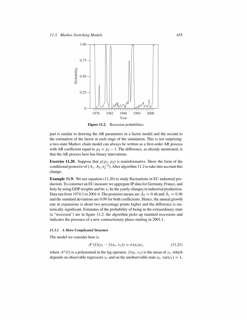
Figure 11.2. Recession probabilities.
part is similar to drawing the AR parameters in a factor model and the second tothe estimation of the factor at each stage of the simulation. This is not surprising:a two-state Markov chain model can always be written as a first-order AR processwith AR coefficient equal to p2 C p1 � 1. The difference, as already mentioned, isthat the AR process here has binary innovations.
Exercise 11.20. Suppose that g.p1; p2/ is noninformative. Show the form of theconditional posterior of .A1; A2; ��2e /. Alter algorithm 11.2 to take into account thischange.
Example 11.9. We use equation (11.20) to study fluctuations in EU industrial pro-duction. To construct an EU measure we aggregate IP data for Germany, France, andItaly by using GDP weights and let yt be the yearly changes in industrial production.Data run from 1974:1 to 2001:4. The posterior means are QA2 D 0:46 and QA1 D 0:96and the standard deviations are 0.09 for both coefficients. Hence, the annual growthrate in expansions is about two percentage points higher and the difference is sta-tistically significant. Estimates of the probability of being in the extraordinary state(a “recession”) are in figure 11.2: the algorithm picks up standard recessions andindicates the presence of a new contractionary phase starting in 2001:1.
11.3.1 A More Complicated Structure
The model we consider here is
Ay.`/.yt � Ny.~t ; xt // D �.~t /et ; (11.21)
where Ay.`/ is a polynomial in the lag operator, Ny.~t ; xt / is the mean of yt , whichdepends on observable regressors xt and on the unobservable state ~t , var.et / D 1,
436 11. Bayesian Time Series and DSGE Models
�.~t / also depends on the unobservable state, and ~t is a two-state Markov chainwith transition matrix P . We set Ny.~t ; xt / D x0tA0 C A1~t , �
2.~t / D �2 C A2~t
and assume A2 > 0, A1 > 0 for identification purposes. Moreover, we restrict theroots of Ay.`/ to be less than 1.
Let yt D .y1; : : : ; yt /, ~t D .~1; : : : ; ~t /; let A be the companion matrixof Ay.`/ and A1 its first m rows. Define � D A2=�
2 and let ˛ D .A0; A1;
A1; �2; �; pij /. The likelihood function is f .yt j ~t ; ˛/ D f .yq j ~q; ˛/ �Qt
�DqC1 f .y� j y��1; ~t�1; ˛/, where the first term is the density of the first q
observations and the second term is the one-step-ahead conditional density of y� .The density of the first q observations (see derivation in the factor model case) is
normal with mean xqA0C~qA1 and variance �2˝q , where˝q D Wq˙qWq ,˙q DA˙qA
0C .1; 0; 0; : : : ; 0/0.1; 0; 0; : : : ; 0/,Wq D diagf.1C �~j /0:5; j D 1; : : : ; qg.Using the prediction error decomposition we have that f .y� j y��1; ~��1; ˛/ /expf�.y� � y� j��1/2=2�2.~� /g, where y� j��1 D .1�Ay.`//yt CAy.`/.x0�A0 CA1~� /. Therefore, yt is conditionally normal with mean yt jt�1 and variance �2.~t /.Finally, the joint density of .yt ; ~t / is f .yt j ~t ; ˛/
Qt�D2 f .~� j ~��1/f .~1/
and the likelihood of the data isRf .yt ; ~t j ˛/ d~t . In chapter 3 we produced
estimates of .˛; ~t / by using a two-step approach: in the first step ˛ML is obtainedby maximizing the likelihood function; in the second step, inference about ~t isobtained conditional on ˛ML. That is,
f .~t ; : : : ; ~t��C1 j yt ; ˛ML/
D
1X~t��D0
f .~t ; : : : ; ~t�� j yt�1; ˛ML/
/ f .~t j ~t�1/f .~t�1; : : : ; ~t�� j yt�1; ˛ML/f .yt j y
t�1; ~t ; ˛ML/;
(11.22)
where the factor of proportionality is given by f .yt j yt�1; ˛ML/ DP~t� � �P
~t��f .yt ; ~t ; : : : ; ~t�� j y
t�1; ˛ML/. Since the log likelihood of the sam-ple is ln f .yqC1; : : : ; yt j yq; ˛/ D
P� ln f .y� j y��1; ˛/, once ˛ML is
obtained, transition probabilities can be computed by using f .~t j yt ; ˛ML/ DR� � �Rf .~t ; : : : ; ~t��C1 j y
t ; ˛ML/ d~t�1 � � � d~t��C1. Note that in this case uncer-tainty in ˛ML is not incorporated in the calculations.
To construct the conditional posteriors of the parameters and of the unobservablestate, assume that g.A0; A1; ��2/ / N. NA0; NA0/N.
NA1; NA1/�.A1>0/G.a�1 ; a
�2 /,
where �.A1>0/ is an indicator function. Further assume that g..1C �/�1/ �G.a1 ; a
2/�.>0/ and g.A1/ � N. NA1; NA1/�.�1;1/, where �.�1;1/ is an indicator for
stationarity. Finally, we letp12 D 1�p11 D 1�p1 andp21 D 1�p22 D 1�p2 andg.pi / / Beta. Ndi1; Ndi2/, i D 1; 2, and assume that all hyperparameters are known.
Exercise 11.21. Let ˛� be the vector ˛ except for and let A D .A0; A1/.
11.3. Markov Switching Models 437
(i) Assuming that the first q observations come from the low state, show that theconditional posteriors for the parameters and the unobserved state are
g.A j yt ; ~t ; ˛�A/ � N. QA; QA/�A1>0;
g.��2 j yt ; ~t ; ˛��2/ � G.a�1 C T; a�2
C .˙�0:5q y �˙�0:5q xA0 C˙�0:5q ~A1/
2/;
g..1C �/�1 j yt ; ~t ; ˛�/ � G.a1 C T1; a2 C rss/�.>0/;
g.A1 j yt ; ~t ; ˛�A1/ � N. QA1; QA1/�.�1;1/j˝qj
�0:5
� expf�.yq � xqA/0˝�1q .yq � xqA/=2�2g;
g.pi j yt ; ~t ; ˛�pi / � Beta. Ndi1 C di1; Ndi2 C di2/; i D 1; 2;
g.~t j yt ; ˛�~�t / / f .~t j ~t�1/f .~tC1 j ~t /
Y�
f .y� j y��1; ~� /;
9>>>>>>>>>>>>>>>>>=>>>>>>>>>>>>>>>>>;(11.23)
where T1 is the number of elements in T for which ~t D 1, dij is the number ofactual transitions from state i to state j , and rss D
PT1tD1fŒ.1� �x
0:5t /.y � x0tA0 �
~tA1/�=2g.(ii) Show the exact form of QA1, QA1 , QA, and QA.(iii) Describe how to draw A1 and A restricted to the correct domain.
Recently, Sims (2001) and Sims and Zha (2004) have used a similar specificationto estimate a Markov switching VAR model, where the switch may occur in thelagged dynamics, in the contemporaneous effects, or in both. To illustrate theirapproach consider the equation
A1.`/it D Ni.~t /C b.~t /A2.`/�t C �.~t /et ; (11.24)
where et � i.i.d. N.0; 1/, it is the nominal interest rate, �t is inflation, and ~t hasthree states with transition
P D
24 p1 1 � p1 0
.1 � p2/=2 p2 .1 � p2/=2
0 1 � p3 p3
35 :The model (11.24) imposes restrictions on the data: the dynamics of interest ratesdo not depend on the state; the form of the lag distribution on �t is the same acrossstates, except for a scale factor b.~/; there is no possibility of jumping from state 1to state 3 (or vice versa) without passing through state 2; finally, the nine elementsof P depend only on three parameters.
Let ˛ D Œvec.A1.`//; vec.A2.`//; Ni.~t /; b.~t /; �.~t /; p1; p2; p3�. The marginallikelihood of the data, conditional on the parameters (but integrating out the unob-servable state) can be computed numerically and recursively. Let Ft be the infor-mation set at t .
Exercise 11.22. Show that f .it ; ~t j Ft�1/ is a mixture of continuous and discretedensities. Show the form off .it j Ft�1/, the marginal of the data, and off .~t j Ft /,the updating density.

438 11. Bayesian Time Series and DSGE Models
Once f .~t j Ft / is obtained we can compute
f .~tC1 j Ft / D
24f .~t D 1 j Ft /f .~t D 2 j Ft /
f .~t D 3 j Ft /
350 Pand from there we can calculate f .itC1; ~tC1 j it ; �t ; : : : /, which makes therecursion complete. Given a flat prior on ˛, the posterior will be proportional tof .˛ j it ; �t / and posterior estimates of the parameters and of the states can imme-diately be obtained.
Exercise 11.23. Provide formulas to obtain smoothed estimates of ~t .
More complicated VAR specifications are possible. For example, let ytA0.~t / D
x0tAC.~t / C et , where xt includes all lags of yt and et � i.i.d. N.0; I /. AssumeAC.~t / D A.~t / C ŒI; 0�0A0.~t /. Given this specification there are two pos-sibilities: either A0.~t / D NA0�.~t / and A.~t / D NA�.~t / or A0.~t / free andA.~t / D NA. In the first specification changes in the contemporaneous and laggedcoefficients are proportional; in the second the state affects the contemporaneousrelationship but not lagged ones.
Equation (11.24) is an equation of a bivariate VAR. Hence, so long as we are ableto keep the posterior of the system in a SUR format (as we have done in chapter 10),the above ideas can be applied to each of the VAR equations.
11.3.2 A General Markov Switching Specification
Finally, we consider a general Markov switching specification which embeds asa special case the two previous ones. So far we have allowed the mean and thevariance of yt to change with the state but we have forced the dynamics to beindependent of the state, apart from a scale effect. This is a strong restriction: infact, it is conceivable that the autocovariance function of the data is different inexpansions and in recessions.
The general two-state Markov switching model we consider is
yt D
(x0tA01 C Y
0tA02 C e0t if ~t D 0;
x0tA02 C Y0tA12 C e1t if ~t D 1;
(11.25)
wherext is a 1�q2 vector of exogenous variables for each t ,Y 0t D .yt�1; : : : ; yt�q1/is a vector of lagged dependent variables and ejt , j D 0; 1, are i.i.d. random vari-ables, normally distributed with mean zero and variance�2j . Once again the transitionprobability for ~t has diagonal elements pi . In principle, some of the elements ofAj i may be equal to zero for some i , so the model may have different dynamics indifferent states.
For identification, we choose the first state to be a “recession”, so thatA02 < A12is imposed. We let ˛c be the parameters which are common across states, ˛i the
11.3. Markov Switching Models 439
parameters which are unique to the state, and ˛i r the parameters which are restrictedto achieve identification. Then (11.25) can be written as
yt D
(X 0ct˛c CX
00t˛0 CX
0rt˛0r C e0t if ~t D 0;
X 0ct˛c CX01t˛1 CX
0rt˛1r C e1t if ~t D 1;
(11.26)
where .X 0ct ; X0it ; X
0rt / D .x
0t ; Y0t / and .˛0c; ˛
0i ; ˛0i r/ D .A
001; A
002; A
011; A
012/.
To construct conditional posteriors for the unknowns we assume conjugate pri-ors: ˛c � N. Nc; Nc/; ˛i � N. N i ; N i /; ˛i r � N. N r; N r/�rest; Ns2i �
�2i � �2. N�i /;
pi � Beta.di1; di2/, i D 1; 2, where �rest is a function indicating whether theidentification restrictions are satisfied. As usual we assume that the hyperparame-ters . Nc; Nc; N i ; N i ; N r; N r; N�i ; Ns2i ;
Ndij / are known or can be estimated from the data.We take the first maxŒq1; q0� observations as given in constructing the posteriordistribution of the parameters and of the latent variable.
Given these priors, it is straightforward to compute conditional posteriors. Forexample, g.˛c j xt ; yt / has mean Qc D Qc.
PTtDminŒq1;q0�
Xcty0ct=�
2t C
N �1c Nc/,
variance Qc D .PTtDminŒq1;q0�
XctX0ct=�
2t C
N �1c /�1, where yct D yt � Xit˛i �
Xrt˛i r and it is normal.
Exercise 11.24. Let Ti be the number of observations in state i .(i) Show that the conditional posterior of ˛i is N. Q i ; Q i /, where ˛i D Q
i �
.PTitD1Xity
0it=�
2t C
N �1i N i /, Q i D .
PTitD1XitX
0it=�
2t C
N �1i /�1, and yit D
yt �Xct˛c �Xrt˛i r.(ii) Show that the conditional posterior of ˛r is N. Q r; Q r/. What are Q r and Q r?(iii) Show that the conditional posterior of ��2i is such that .Ns2i C rss2i /=�
2i �
�2.�i C Ti �maxŒq1; q2�/. Write down the expression for rss2i .(iv) Show that the conditional posterior for pi is Beta. Ndi1 C di1; Ndi2 C di2/.
Finally, the conditional posterior for the latent variable ~t can be computedas usual. Given the Markov properties of the model, we restrict attention to thesubsequence ~t;� D .~t ; : : : ; ~tC��1/. Define ~t.��/ as the sequence ~t withthe � th subsequence removed. Then g.~t;� j y; ~t.��// / f .y j ~t ; ˛; �
2/ �
g.~t;� j ~t.��/; pi /, which is a discrete distribution with 2� outcomes. Usingthe Markov property, g.~t;� j ~t.��/; pi / D g.~t;� j ~t�1; ~tC� ; pi / whilef .yT j ~t ; ˛/ /
QtC��1jDt .1=�j / expf�e2j =2�
2j g. Note that, since the ~t are cor-
related, it is a good idea to choose � > 1.
Exercise 11.25. Write down the components of the conditional posterior for ~twhen � D 1.
In all Markov switching specifications, it is important to wisely select the initialconditions. One way to do so is to assign all the observations in the training sample toone state, obtain initial estimates for the parameters, and arbitrarily set the parametersof the other state to be equal to the estimates plus or minus a small number (say, 0.1).Alternatively, one can split the points arbitrarily but equally across the two states.
440 11. Bayesian Time Series and DSGE Models
Exercise 11.26. Suppose�yt D ˛0C˛1�yt�1Cet ; et � i.i.d. N.0; �2e / if ~t D 0and �yt D .˛0 C A0/ C .˛1 C A1/�yt�1 C et , et � i.i.d. N.0; .1 C A2/�
2e / if
~t D 1. Using quarterly GDP growth data for the euro area, construct posteriorestimates for A0; A1; A2. Separately test if there is evidence of switching in theintercept, the dynamics, or the variance of �yt .
11.4 Bayesian DSGE Models
The use of Bayesian methods to estimate and evaluate Dynamic Stochastic GeneralEquilibrium (DSGE) models does not present new theoretical aspects. We haverepeatedly mentioned that DSGE models are false in at least two senses.
� They only provide an approximate representation to the DGP of the actualdata. In particular, since the vector of structural parameters is typically of lowdimension, strong restrictions are implied both in the short and in the longrun.
� The number of driving forces is smaller than the number of endogenous vari-ables so that the covariance matrix of a vector of variables generated by themodel is singular.
These features make the estimation and testing of DSGE models with GMM or MLtricky. In fact, with these methods inference is (asymptotically) justified only whenthe model is the DGP of the data up to a set of unknown parameters, while stochasticsingularity prevents numerical routines based on the Hessian from working properlyin the search for the maximum of the objective function. In chapter 4 we describeda minimalist approach, which only uses qualitative restrictions to identify shocksin the data, and can be employed to examine the match between the theory and thedata, when the model is false in the two above senses.
Bayesian methods are also well-suited to dealing with false models. Posteriorinference, in fact, does not hinge on the model being the correct DGP and it isfeasible even when the covariance matrix of the vector of endogenous variables issingular — we do not need the Hessian to explore the shape of the posterior. Bayesianmethods have another advantage over alternatives, which makes them appealing tomacroeconomists. Posterior distributions in fact incorporate uncertainty about theparameters and the model specification.
Since log-linearized DSGE models are state space models with nonlinear restric-tions on the mapping between reduced-form and structural parameters, posteriorestimates of the structural parameters can be obtained, for appropriately designedprior distributions, by using the posterior simulators described in chapter 9. Given thenonlinearity of the mapping, Metropolis, or MH algorithms are generally employed.Numerical methods can also be used to compute marginal likelihoods and Bayesfactors; to obtain any posterior function of the structural parameters (for example,impulse responses, variance decompositions, ACFs, turning-point predictions, and

11.4. Bayesian DSGE Models 441
forecasts) and to examine the sensitivity of the results to variations in the prior spec-ification. Once the posterior distribution of the structural parameters is obtained,any interesting inferential exercise becomes trivial.
To estimate the posterior for the structural parameters and for the statistics of inter-est, and to evaluate the quality of a DSGE model, the following steps are typicallyused.
Algorithm 11.3.
(1) Construct a log-linear approximation to the DSGE economy and transform itinto a state space model.Add measurement errors if the dimension of the vectorof endogenous variables used in estimation/evaluation exceeds the dimensionof the vector of driving forces of the model.
(2) Specify prior distributions for the structural parameters � .
(3) Perform prior analysis to study the range of potential outcomes of the model.
(4) Draw sequences from the joint posterior of � by using Metropolis or MHalgorithms. Check convergence.
(5) Compute marginal likelihood numerically by using draws from the prior dis-tribution and the Kalman filter. Compute the marginal likelihood for anyalternative or reference model. Calculate Bayes factors or other measures of(relative) forecasting fit.
(6) Construct statistics of economic interest by using the draws in (4) (after aninitial set has been discarded). Use loss-based measures to evaluate the dis-crepancy between the theory and the data.
(7) Examine the sensitivity of the results to the choice of priors.
Step (1) is unnecessary. We will see later on what to do if a nonlinear specificationis used. Adding measurement errors helps computationally to reduce the singularityof the covariance matrix of the endogenous variables but it is not needed for theapproach to work.
In step (2) prior distributions are generally centered around standard values ofthe parameters, while standard errors typically reflect subjective prior uncertainty.One could also specify objective prior standard errors, so as to “cover” the rangeof existing estimates, as we have done in chapter 7. For convenience, the priordistribution for the vector of parameters is assumed to be the product of univariatedistributions of each of the parameters. In some applications, it may be convenient toselect diffuse priors over a fixed range to avoid imposing too much structure on thedata. In general, the form of the prior reflects computational convenience. Conjugatepriors are typically preferred. For parameters which must lie in an interval, truncatednormal or beta distributions are often chosen.
Step (3) logically precedes posterior analysis and can be used to evaluate whethermodels have any chance of producing the interesting features we observe in theactual data. This is precisely the analysis we performed in chapter 7, where we
442 11. Bayesian Time Series and DSGE Models
compare statistics of the data with the range of statistics produced by models. Whilethis step is often skipped, it may provide very useful information about the potentialoutcomes of the models.
Step (4) requires choosing an updating rule and a transition function P.�†; � l�1/
satisfying the regularity conditions described in chapter 9, estimating joint andmarginal distributions by using kernel methods and the draws from the posterior,and checking convergence. In particular, the following steps are needed.
Algorithm 11.4.
(i) Given a �0, draw �† from P.�†; �0/, and compute the prediction error decom-position of the likelihood, i.e., estimate f .y j �0/ and f .y j �†/.
(ii) Evaluate the posterior kernel at �† and �0, i.e., calculate Mg.�†/ D f .y j �†/�
g.�†/ and Mg.�0/ D f .y j �0/g.�0/.
(iii) Draw U � U.0; 1/. If U < minfŒ. Mg.�†/= Mg.�0//�ŒP.�0; �†/=P.�†; �0/�; 1g,set �1 D �†, otherwise set �1 D �0.
(iv) Repeat steps (i)–(iii) NLC JL times. Discard the first NL draws, keep one drawevery L for inference. Alternatively, repeat steps (i)–(iii) J times by usingNLC 1 different �0, and keep the last draw from each run. Check convergenceby using the methods described in chapter 9.
(v) Estimate marginal/joint posteriors with kernel methods. Compute locationestimates and credible sets. Compare them with those computed from theprior.
Step (5) requires drawing parameters from the prior, calculating the sequence ofprediction errors for each draw, and averaging over draws. To do so, one could usethe modified harmonic mean, f.1=L/
Pl Œg
IS.��/=f .y j ��/g.��/�g�1, suggestedby Gelfand and Dey (1994), where �� is a point with high posterior probability andgIS is a density with tail thinner than f .y j �/g.�/, or could use the Bayes theoremdirectly, as suggested by Chib (1995). Similar calculations can be undertaken forany alternative model and Bayes factors can then be numerically computed. Whenthe dimensionality of the parameter space is large, Laplace approximations canreduce the computational burden and give a more accurate picture of the propertiesof various models. The competitors could be a structural model, which nests the oneunder consideration (e.g., a model with flexible prices can be obtained by restrictingone parameter of a model with sticky prices), a nonnested structural specification(e.g., a model with sticky wages), or a more densely parametrized reduced-formmodel (e.g., a VAR or a BVAR).
In step (6) loss functions are needed to compare statistics of interest becauseDSGE models typically have low posterior probability. As we will see later on,posterior odds ratios may not be very informative in such a case.
In step (7), to check the robustness of the results to the choice of prior, one canreweigh the posterior draws by using the techniques described in section 9.5.
11.4. Bayesian DSGE Models 443
11.4.1 Identification
Since log-linearized DSGE models feature a nonlinear mapping between the param-eters of the theory and those of the state space representation, and since there is nocondition that can be easily employed to check the informational content of thedata, any method which is concerned with the estimation of DSGE parameters mustdeal with potential identification problems. We have already seen aspects of suchphenomena in chapters 5 and 6, when dealing with (classical) impulse responsematching and maximum likelihood estimation. Since Bayesian inference is basedon the likelihood principle, and since the model structure determines, to a largeextent, whether parameters are identified or not, all the arguments previously madealso apply to a Bayesian context. However, Bayesian methods have two importantadvantages over classical ones in the presence of identification problems: they canemploy information from other data sets to reduce parameter underidentification;they can generate coherent inference even in the presence of identification problems.
Suppose that � D Œ�1; �2�, assume that� D �1 ��2, and suppose that the like-lihood function has no information for �2, i.e., f .y j �/ D f �.y j �1/. Straight-forward application of the Bayes theorem implies that g.� j y/ D g.�1 j y/ �
g.�2 j �1/ / f�.y j �1/g.�1; �2/. Hence, a proper prior for � can add curvature
to a flat likelihood function. This facilitates both the maximization of the poste-rior, if needed, and its calculations with MCMC methods, and makes the posteriorwell-behaved. Nevertheless, there is no updating of the prior of �2 j �1. Hence,a comparison of the prior and the posterior of � can indicate how informative thedata are (priors and posteriors of identified parameters will be different, priors andposteriors of unidentified parameters will not). Furthermore, a sequence of priordistributions with different spreads can be used to assess the extent of identificationproblems. In fact, the posterior of parameters with dubious identification featureswill become more and more diffuse, while the posterior of identified parameters willhardly change.
When the space of parameters� is not variation free, i.e.,� ¤ �1��2, becauseof stability constraints or restrictions required for the solution to the model to gener-ate nonimaginary time series, the prior of �2 could be marginally updated even whenthe likelihood has no information, since changes in the distribution of �2 imply thatthe domain of �1 changes (see, for example, Poirier 1998). In this situation, a com-parison of priors and posteriors will not be informative about potential identificationproblems, unless the parameters constrained by economic requirements are known.This is unlikely to be true in DSGE setups since, for example, the eigenvalues whichregulate stability are complicated functions of all the parameters of the model.
Complete lack of identification is typically limited to textbook examples. How-ever, partial or weak identification problems are extremely common. Partial identi-fication occurs when the likelihood displays a ridge in some dimension (see exam-ple 6.21), while weak identification implies that the likelihood function is flat insome or all dimensions. Both these phenomena are difficult to detect in practice

444 11. Bayesian Time Series and DSGE Models
0.010.02
0.03
0.985
0.990
0.995
β0.01
0.020.03
0.985
0.990
0.995
4
3
2
1
0
β
20
15
10
5
0×104
×104
δ δ
Figure 11.3. Likelihood and posterior, RBC model.
since, in the first case, it is the joint posterior which is indistinguishable from thejoint prior (univariate posteriors may move away from univariate priors), while, inthe second case, the size of the differences between the priors and the posteriorsmay depend on the details of MCMC routine employed.
As mentioned, well-behaved priors can induce well-behaved posteriors, evenwhen the data have no information about the parameters. Therefore, it is very impor-tant that the priors of potentially nonidentifiable parameters truly contain informa-tion external to the data used to estimate the model and effectively reflect the objec-tive uncertainty a researcher faces in specifying it. When these two general principlesare not followed, Bayesian inference can mask rather than highlight identificationproblems. In fact, a sufficiently tight prior may give the illusion that parameterestimation is successful, that the model fits the data well, therefore creating thepreconditions for its use for policy purposes. We show how this can occur with themodel of example 6.21, which has a likelihood function with both flat sections andridges.
Example 11.10. Figure 11.3 reproduces the likelihood function presented in thesecond panel of figure 6.1, which we have seen displays a ridge in ˇ; ı running from(ı D 0:005, ˇ D 0:975) up to .ı D 0:03, ˇ D 0:99/, and presents the joint posteriorfor these two parameters, when a sufficiently tight prior on ı is used. Clearly, whilethe likelihood has a diagonal ridge, the posterior appears to be much better behaved,since there is very low prior probability that ı lies outside the range .0:018; 0:025/.
While there may be reasonable economic arguments for a priori limiting thesupport of ı, they should be clearly spelled out. Furthermore, when bounds areimposed, the prior should be made reasonably uninformative to avoid misleadingconclusions. Note that centering estimates at standard calibrated values is not thebest strategy to follow since such values are likely to have been obtained with thesame data that is employed for estimation, making the prior too data based.
11.4. Bayesian DSGE Models 445
11.4.2 Examples
Next, we present a few examples, highlighting the practical details of the imple-mentation of Bayesian methods for inference in DSGE models.
Example 11.11. The first example is simple. We simulate data from a basic RBCmodel where the solution is contaminated by measurement errors. Armed with rea-sonable prior specifications for the structural parameters and a Metropolis algorithm,we examine where the posterior distribution of some crucial parameters lies rela-tive to the “true” parameters we used in the simulations, when samples typical inmacroeconomic data are available. We also compare true and estimated moments togive an economic measure of the fit we obtain.
The solution to an RBC model driven by i.i.d. technological disturbances whencapital depreciates instantaneously, leisure does not enter the utility function, andthe latter is logarithmic in consumption is
KtC1 D .1 � /ˇK1��t �t C v1t ; (11.27)
GDPt D K1��t �t C v2t ; (11.28)
ct D ˇGDPt C v3t ; (11.29)
rt D .1 � /GDPtKt
C v4t : (11.30)
We have added four measurement errorsvjt , j D 1; 2; 3; 4, to the equations to reducethe singularity of the system and to mimic the typical situation an investigator islikely to face. Here ˇ is the discount factor, 1� the share of capital in production.We simulate 1000 data points by using k0 D 100:0, .1 � / D 0:36, ˇ D 0:99,ln �t � N.0; �2
D 0:1/, v1t � N.0; 0:06/, v2t � N.0; 0:02/, v3t � N.0; 0:08/,
v4t � U.0; 0:1/, and keep only the last 160 data points to reduce the dependenceon the initial conditions and match a typical sample size.
We treat �2
as fixed and focus attention on the two economic parameters. Weassume that the priors are .1� / � Beta.4; 9/ and ˇ � Beta.99; 2/. Beta distribu-tions are convenient because they are easy to draw from. In fact, if x � �2.2a/ andy � �2.2b/, then z D x=.x C y/ � Beta.a; b/. Since the mean of a Beta.a; b/ is.a=aC b/ and the variance is ab=Œ.aC b/2.aC bC 1/�, the prior mean of 1� isabout 0.31, and the prior mean of ˇ about 0.99. The variances, approximately equalto 0.011 and 0.0002, imply sufficiently loose prior distributions.
We draw 10 000 replications. Given 1 � 0 D 0:55, ˇ0 D 0:97, we producecandidates �† D Œ.1 � /†; ˇ†� by using a reflecting random walk process, i.e.,�† D N� C .� l�1 � N�/C vl
�, where � l�1 is the previous draw, N� is the mean of the
process and vl�
is a vector of errors. The first component of v� (corresponding to1� ) is drawn from a U.�0:03; 0:03/ and the second (corresponding to ˇ) from aU.�0:01; 0:01/ and N� D Œ0:01; 0:001�0. These ranges produce an acceptance rate ofabout 75%.
Since we are interested in .1� / andˇ, we are free to select which equations to useto estimate them. We arbitrarily choose those determining consumption and the real

446 11. Bayesian Time Series and DSGE Models
0.1 0.2 0.3 0.4 0.5 0.6 0.70
1
2
3
4
5
6PriorPosterior
0.900 0.925 0.950 0.975 1.0000
5
10
15
20
25
30
35
40PriorPosterior
1 − βη
Figure 11.4. Priors and posteriors, basic RBC.
Table 11.2. Variances and covariances.
True Posterior 68% range
var.c/ 40.16 Œ3:65; 5:10 � 1010�
var.r/ 1:29 � 10�5 Œ2:55 � 10�4; 136:11�
cov.c; r/ �0:0092 Œ�0:15 � 10�5;�0:011�
interest rate. We assume a normal likelihood and since g.1� ; ˇ/ D g.1� /g.ˇ/,we calculate the prior at the draw for each of the two parameters separately. Sincethe transition matrix P.�†; �0/ is symmetric, the ratio of the kernels at �† and � l�1
is all that is needed to accept or reject the candidates.We discard the first 5000 draws. Out of the last 5000 we keep 1 out of every 5
to reduce the serial correlation present in the draws. We check that the Metropolisalgorithm has converged in two ways: splitting the sequences of draws in two andcomputing a normal test; calculating recursive means for the estimates of eachparameter. In both cases, the sequence converged after about 2000 draws.
Figure 11.4 presents the marginal densities of 1� andˇ, estimated with the 1000saved draws from the prior and the posterior. Two features are worth mentioning.First, the data are more informative about 1� than they are about ˇ. Second, bothposteriors are unimodal and roughly centered around the true parameter values.
Using the 1000 posterior draws we have calculated three statistics, the variancesof consumption and of the real interest rate and the covariance between the two, andcompared the posterior 68% credible range with the statistics computed by usingthe “true” parameters. Table 11.2 shows that the posterior 68% range includes theactual value of the consumption variance but not the one for the real rate or for the
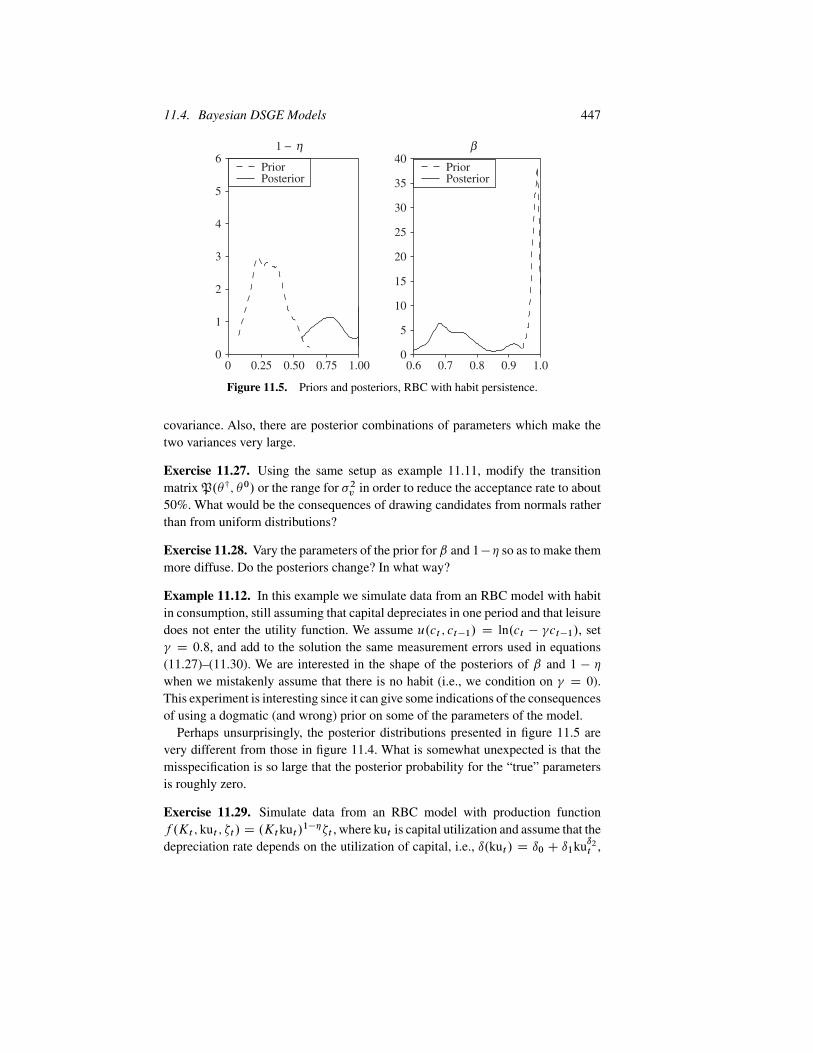
11.4. Bayesian DSGE Models 447
0 0.25 0.50 0.75 1.000
1
2
3
4
5
6
0.6 0.7 0.8 0.9 1.0
PriorPosterior
0
5
10
15
20
25
30
35
40PriorPosterior
1 − βη
Figure 11.5. Priors and posteriors, RBC with habit persistence.
covariance. Also, there are posterior combinations of parameters which make thetwo variances very large.
Exercise 11.27. Using the same setup as example 11.11, modify the transitionmatrix P.�†; �0/ or the range for �2v in order to reduce the acceptance rate to about50%. What would be the consequences of drawing candidates from normals ratherthan from uniform distributions?
Exercise 11.28. Vary the parameters of the prior for ˇ and 1� so as to make themmore diffuse. Do the posteriors change? In what way?
Example 11.12. In this example we simulate data from an RBC model with habitin consumption, still assuming that capital depreciates in one period and that leisuredoes not enter the utility function. We assume u.ct ; ct�1/ D ln.ct � �ct�1/, set� D 0:8, and add to the solution the same measurement errors used in equations(11.27)–(11.30). We are interested in the shape of the posteriors of ˇ and 1 � when we mistakenly assume that there is no habit (i.e., we condition on � D 0).This experiment is interesting since it can give some indications of the consequencesof using a dogmatic (and wrong) prior on some of the parameters of the model.
Perhaps unsurprisingly, the posterior distributions presented in figure 11.5 arevery different from those in figure 11.4. What is somewhat unexpected is that themisspecification is so large that the posterior probability for the “true” parametersis roughly zero.
Exercise 11.29. Simulate data from an RBC model with production functionf .Kt ; kut ; �t / D .Ktkut /1���t , where kut is capital utilization and assume that thedepreciation rate depends on the utilization of capital, i.e., ı.kut / D ı0 C ı1kuı2t ,

448 11. Bayesian Time Series and DSGE Models
where ı0 D 0:01, ı1 D 0:005, ı2 D 2. Suppose you mistakenly neglect utiliza-tion and estimate a model like the one in equations (11.27)–(11.30). Evaluate thedistortions induced by this misspecification.
Example 11.13. The next example considers a standard New Keynesian modelwith sticky prices and monopolistic competition. Our task here is twofold. First,we want to know how good this model is relative to, say, an unrestricted VAR incapturing the dynamics of the nominal interest rate, the output gap, and inflation.Second, we are interested in knowing the location of the posterior distribution ofsome important structural parameters. For example, we would like to know howmuch price stickiness is needed to match actual dynamics, whether policy inertia isan important ingredient to characterize the data, and whether the model has someinternal propagation mechanism or if, instead, it relies entirely on the dynamics ofthe exogenous variables to match the dynamics of the data.
The model economy we use is a simplified version of the structure considered inchapter 2 and comprises a log-linearized (around the steady-state) Euler equation,a New Keynesian Phillips curve, and a Taylor rule. We assume that, in equilibrium,consumption is equal to output and use output in deviation from steady states inthe Euler equation directly. Each equation has a shock attached to it: there is ani.i.d. policy shock, �3t , a cost push shock in the Phillips curve, �2t , and an arbitrarydemand shock in the Euler equation, �4t . While the latter shock is unnecessary forthe estimation, it is clearly needed to match the complexities of the output, inflation,and interest rate processes observed in the real world. The equations are
gdpgapt D Et gdpgaptC1 �1
'.it �Et�tC1/C �4t ; (11.31)
�t D ˇEt�tC1 C � gdpgapt C �2t ; (11.32)
it D r it�1 C .1 � r /.��t�1 C gap gdpgapt�1/C �3t ; (11.33)
where it is the nominal interest rate, �t is the inflation rate, gdpgapt is the outputgap, � D .1� �p/.1� ˇ�p/.' C #N /=�p, �p is the degree of stickiness in the Calvosetting, ˇ is the discount factor, ' is the risk aversion parameter, #N is the inverseelasticity of labor supply, r is the persistence of the nominal rate, while � andgap measure the responses of interest rates to lagged inflation and lagged outputgap movements. We assume that �4t and �2t are AR(1) processes with persistence4; 2 and variances �24 ; �
22 , while �3t is i.i.d. .0; �23 /.
The model has 12 parameters, � D .ˇ; '; #; �p; � ; gap; r ; 2; 4; �22 ; �
23 ; �
24 /,
seven structural, and five auxiliary ones, whose posterior distributions need tobe found. Our interest centers in the posterior distributions of .�p; r ; 2; 4/. Itis easy to check that �p and #N are not separately identifiable so that inferenceabout �p will be meaningful only to the extent that the priors of these two param-eters are carefully specified. We use U.S. quarterly detrended data from 1948:1to 2002:1. We assume that g.�/ D
Q12jD1 g.�j / and use the following priors:
ˇ � Beta.98; 3/; ' � N.1; .0:375/2/; #N � N.2; .0:75/2/; �p � Beta.9; 3/; r �
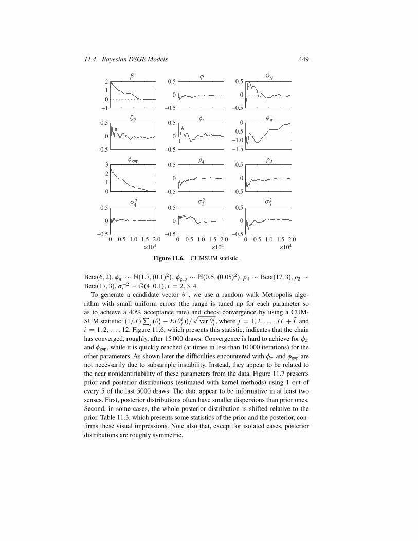
11.4. Bayesian DSGE Models 449
p
0
1
2
3
β
×1040 0.5 1.0 1.5 2.0
×1040 0.5 1.0 1.5 2.0
×1040 0.5 1.0 1.5 2.0
−0.5
0
0.5
−0.5
0
0.5
−0.50
−1.5−1.0
−0.5
0
0.5
−0.5
0
0.5
−0.5
0
0.5
−0.5
0
0.5
−0.5
0
0.5
−0.5
0
0.5
−0.5
0
0.5
−1012
ζ
gapφ
4σ 3σ2σ
4ρ 2ρ
ϕ Nϑ
rφ φπ
2 22
Figure 11.6. CUMSUM statistic.
Beta.6; 2/; � � N.1:7; .0:1/2/; gap � N.0:5; .0:05/2/; 4 � Beta.17; 3/; 2 �Beta.17; 3/, ��2i � G.4; 0:1/, i D 2; 3; 4.
To generate a candidate vector �†, we use a random walk Metropolis algo-rithm with small uniform errors (the range is tuned up for each parameter soas to achieve a 40% acceptance rate) and check convergence by using a CUM-SUM statistic: .1=J /
Pj .�
ij �E.�
ij //=p
var � ij , where j D 1; 2; : : : ; JLC NL andi D 1; 2; : : : ; 12. Figure 11.6, which presents this statistic, indicates that the chainhas converged, roughly, after 15 000 draws. Convergence is hard to achieve for �and gap, while it is quickly reached (at times in less than 10 000 iterations) for theother parameters. As shown later the difficulties encountered with � and gap arenot necessarily due to subsample instability. Instead, they appear to be related tothe near nonidentifiability of these parameters from the data. Figure 11.7 presentsprior and posterior distributions (estimated with kernel methods) using 1 out ofevery 5 of the last 5000 draws. The data appear to be informative in at least twosenses. First, posterior distributions often have smaller dispersions than prior ones.Second, in some cases, the whole posterior distribution is shifted relative to theprior. Table 11.3, which presents some statistics of the prior and the posterior, con-firms these visual impressions. Note also that, except for isolated cases, posteriordistributions are roughly symmetric.

450 11. Bayesian Time Series and DSGE Models
Table 11.3. Prior and posterior statistics.
Prior Posterior 1948–2002‚ …„ ƒ ‚ …„ ƒMean Std Median Mean Std Min Max
ˇ 0.98 0.01 0.978 0.976 0.007 0.952 0.991
' 0.99 0.37 0.836 0.841 0.118 0.475 1.214
#N 2.02 0.75 1.813 2.024 0.865 0.385 4.838
�p 0.75 0.12 0.502 0.536 0.247 0.030 0.993
r 0.77 0.14 0.704 0.666 0.181 0.123 0.992
� 1.69 0.10 1.920 1.945 0.167 1.568 2.361
gap 0.49 0.05 0.297 0.305 0.047 0.215 0.410
4 0.86 0.07 0.858 0.857 0.038 0.760 0.942
2 0.86 0.07 0.842 0.844 0.036 0.753 0.952
�24 0.017 0.01 0.017 0.017 0.007 0.001 0.035
�22 0.016 0.01 0.011 0.012 0.008 0.0002 0.036
�23 0.017 0.01 0.015 0.016 0.007 0.001 0.035
Posterior Posterior1948–1981 1982–2002‚ …„ ƒ ‚ …„ ƒ
Mean Std Mean Std
ˇ 0.986 0.008 0.983 0.008
' 1.484 0.378 1.454 0.551
#N 2.587 0.849 2.372 0.704
�p 0.566 0.200 0.657 0.234
r 0.582 0.169 0.695 0.171
� 2.134 0.221 1.925 0.336
gap 0.972 0.119 0.758 0.068
4 0.835 0.036 0.833 0.036
2 0.831 0.036 0.832 0.036
�24 0.017 0.006 0.016 0.007
�22 0.016 0.006 0.016 0.007
�23 0.013 0.007 0.014 0.007
As far as the posterior of the four parameters of interest is concerned, note thatthe shocks are persistent (the posterior mean is 0.85) but there is no pileup of theposterior distribution for the AR parameters around 1. This means that, although themodel does not have sufficient internal propagation to replicate the dynamics of thedata, no exogenous unit-root-like processes are needed.
The posterior distribution of economic parameters is reasonably centered. Theposterior mean of �p, the parameter regulating the stickiness in prices, is only 0.5,
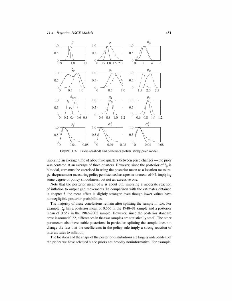
11.4. Bayesian DSGE Models 451
0.9 1.0 1.1 0 0.5 1.0 1.5 2.0 0 2 4 6
0 0.5 1.0 0 0.5 1.0 1.5 2.0 2.5
0 0.2 0.4 0.6 0.8 0.6 0.8 1.0 1.2 0.6 0.8 1.0 1.2
0 0.04 0.08 0 0.04 0.08 0 0.04 0.08
0
0.5
1.0
0
0.5
1.0
0
0.5
1.0
0
0.5
1.0
0
0.5
1.0
0
0.5
1.0
0
0.5
1.0
0
0.5
1.0
0
0.5
1.0
0
0.5
1.0
0
0.5
1.0
0
0.5
1.0
p
β
ζ
gapφ 4ρ 2ρ
ϕ Nϑ
rφ φπ
4σ 3σ2σ 2 22
Figure 11.7. Priors (dashed) and posteriors (solid), sticky price model.
implying an average time of about two quarters between price changes — the priorwas centered at an average of three quarters. However, since the posterior of �p isbimodal, care must be exercised in using the posterior mean as a location measure.r , the parameter measuring policy persistence, has a posterior mean of 0.7, implyingsome degree of policy smoothness, but not an excessive one.
Note that the posterior mean of � is about 0.5, implying a moderate reactionof inflation to output gap movements. In comparison with the estimates obtainedin chapter 5, the mean effect is slightly stronger, even though lower values havenonnegligible posterior probabilities.
The majority of these conclusions remain after splitting the sample in two. Forexample, �p has a posterior mean of 0.566 in the 1948–81 sample and a posteriormean of 0.657 in the 1982–2002 sample. However, since the posterior standarderror is around 0.22, differences in the two samples are statistically small. The otherparameters also have stable posteriors. In particular, splitting the sample does notchange the fact that the coefficients in the policy rule imply a strong reaction ofinterest rates to inflation.
The location and the shape of the posterior distributions are largely independent ofthe priors we have selected since priors are broadly noninformative. For example,

452 11. Bayesian Time Series and DSGE Models
reweighing the posterior draws with a prior whose range is 90% of the range ofthe original prior in all 12 dimensions produces posterior distributions which arequalitatively very similar to those of figure 11.7.
Finally, we examine the forecasting performance of the model by comparing itsmarginal likelihood to that of a VAR(3) and that of a BVAR(3) with Minnesota priorand standard parameters (tightness equal to 0.1, linear lag decay and weight on othervariables equal to 0.5), both with a constant. Bayes factors are small (of the order of0.19) in both cases, indicating that the model can be improved upon in a forecastingsense. Note that, while both alternatives are more densely parametrized than ourDSGE model (30 versus 12 parameters), Bayes factors take model size into accountand no adjustment for the number of parameters is needed.
Exercise 11.30. Repeat the estimation of the model of example 11.13 by substituting(11.33) with the rule it D r it�1C .1�r /.��t Cgapgdpgapt /C �3t . Comparethe results. In particular, describe how the posterior distributions of r , 2, and 4are altered. Evaluate the probability that the data have been generated by a modelwith indeterminacies (i.e., evaluate what is the posterior probability that � < 1).(Hint: set the location of the prior for � to 1.0.)
Exercise 11.31. Consider the model of example 11.13, but replace the Phillips curveby the following:�t D Œ!=.1C!ˇ/��t�1C Œˇ=.1C!ˇ/�Et�tC1C Œ�=.1C!ˇ/��gdpgapt C �2t , where ! is the degree of indexation of prices. Estimate this modeland test whether indexation is necessary to match the data. (Hint: be careful aboutthe identification of this parameter.)
Exercise 11.32. Add to the model of example 11.13 the following wage equation:�wt D ˇEt�wtC1 C Œ.1 � �w/.1 � �wˇ/=�w.1 C &w#N /�Œmrst � .wt � pt /� C�2t , where �w is the probability of not changing the wage, &w is the elasticity ofsubstitution between types of labor in production, and mrst is the marginal rate ofsubstitution. Estimate this model and test whether wage stickiness adds to the fit ofthe basic sticky price model.
11.4.3 A Few Applied Tips
Although the models we have considered so far are of small scale, it has becomestandard in central banks and international institutions to estimate large-scale DSGEmodels with Bayesian methods. Care should be exercised when estimating large-scale models for several reasons.
First, large-scale models, while more articulate and potentially less misspeci-fied, are more prone to identification problems. Furthermore, the variables used inestimation need not carry information about the parameters researchers care about.For example, it is quite common to try to get estimates of import and export pricestickiness by using CPI inflation of different countries. Obviously, the informationalcontent of CPI inflation for these parameters may be very small.
11.4. Bayesian DSGE Models 453
Second, as we have seen in chapter 6, the likelihood function of a small-scaleDSGE model may have large flat sections or very rocky appearance. The likeli-hood function of a large-scale DSGE model typically contains both features and,at times, multiple peaks may be present. Calculation of posterior distributions insuch a situation is difficult and the prior plays a crucial role in making inferencepossible. Hence, the choice of prior distributions should be carefully documented,the sensitivity of the results to variations in the spread presented, and the temptationto use reverse engineering (i.e., set a prior so that the posterior is well-behaved andconfirms one’s “gut” feeling) avoided. Note that multiple peaks in the likelihoodmay indicate the presence of breaks or multiple regimes and may give importantinformation about features one is interested in examining. Once again, robustnessanalysis may inform the investigator on the likely presence of these problems.
Third, while it is common to start from a model with a large number of frictionsand shocks, Bayesian methods can be used even with models which are misspec-ified in their dynamics or their probabilistic nature. This means that the type ofsequential exercise performed in early calibration exercises (e.g., start from a com-petitive structure with only technology shocks, add government shocks, introducenoncompetitive markets, etc.) can also be fruitfully employed here. Frictions andshocks which add little to the ability of the model to reproduce interesting featuresof the data should be discarded. Such an analysis could also help to give some of theblack-box shocks estimated in the factor literature an interesting economic content.
Finally, models are hardly built to explain the macroeconomic series that onefinds in standard databanks. Therefore, data transformations, such as detrending oroutlier elimination, and massaging techniques, such as the selection of appropriatelystable sample periods or the elimination of structural breaks, are necessary beforethe model is taken to the data. When one is interested in the estimation of a modeldesigned to capture only the cyclical properties of the data and dogmatically selectsone trend specification, Bayesian and standard classical methods face the samearbitrariness problems and everything we said in chapter 3 applies without change.If more than one alternative trend specification is contemplated, one could put a prioron the various alternatives, compute the posterior probability of each specification,and use the techniques described in the next subsection to undertake inference.
11.4.4 Comparing the Quality of Models to the Data
While Bayesian estimation of structural parameters is simple, it is less straightfor-ward to compare the model outcomes to the actual data and to assess the superiorityof a model among alternative candidate specifications. Two methods are available.The first, preferred by macroeconomists, is based on informal analysis of someinteresting economic statistics.
Example 11.14. Continuing with example 11.13, we present 68% impulse responsebands to interest rate shocks in figure 11.8. While responses are economically rea-sonable there are three features of the figure which stand out. First, shocks which

454 11. Bayesian Time Series and DSGE Models
Output gap
0 5 10Horizon (quarters)
Inflation
0 5 10
Nominal rate
−0.5
0
0.5
1.0
−6
−5
−4
−3
−2
−1
0
−2.5
−2.0
−1.5
−1.0
−0.5
0
5 100
Figure 11.8. Responses to monetary shocks, 1948–2002.
increase interest rates make inflation and the output gap fall with very high prob-ability. Second, responses die out after a few periods. Third, despite the assumedprice stickiness, the largest inflation effect is instantaneous.
Figure 11.9 reports response bands obtained by estimating the model over dif-ferent windows of data, keeping a constant number of observations in each sample.It is remarkable that the sign, the shape, and the magnitude of the posterior 68%credible bands are unchanged as we move from the late 1970s to the early 2000s.Hence, the transmission properties of monetary shocks have hardly changed overthe last 30 years.
As an alternative to the presentation of economic statistics of various nestedor nonnested models, one could compute measures of forecasting performance ofvarious specifications. As we have seen in chapter 9, the marginal likelihood is theproduct of one-step-ahead forecast errors. Hence, selecting a model by using Bayesfactors, as we did in example 11.13, is equivalent to choosing the specificationwith smallest one-step (in-sample) MSE. Clearly, out-of-sample forecasting racesare also possible, in which case predictive Bayes factors can be computed (see, forexample, DeJong et al. 2000). This is easy to do: we leave it to the reader to workout the details.
Exercise 11.33. Show how to construct the predictive density of future ytC� ,� D 1; 2; : : : , given the model of example 11.13. (Hint: use the restricted VARrepresentation of the model.)
Despite their popularity, Bayes factors may not be very informative about thequality of the approximation of the model to the data, in particular, when the modelsone wishes to compare are grossly misspecified.
Example 11.15. Suppose there are three models, two structural ones (M1, M2)and a densely parametrized (e.g., a VAR) reference one (M3). The Bayes factorbetween the two structural models is Œf .y;M1/=f .y/� � Œf .y/=f .y;M2/�, where

11.4. Bayesian DSGE Models 455
f .y/ DRf .y;Mi / dMi . If we use a 0–1 loss function, and assume that the prior
probability of each model is 0.5, the posterior risk is minimized by selecting M1 ifthe Bayes factor exceeds 1. The presence of a third model does not affect the choicesince it only enters in the calculation of f .y/, which cancels out of the Bayes factor.If the prior odds do not depend on this third model, the posterior odds ratio will alsobe independent of it.When M1 and M2 are misspecified, they will have low posteriorprobability relative to M3, but this has no influence on the inference one makes.Hence, comparing misspecified models with a Bayes factor may be uninteresting:one model may be preferable to another but it may have close to zero posteriorprobability.
Schorfheide (2000) provided a simple procedure to choose among misspecifiedmodels (in his case a cash-in-advance and a working-capital model). The actual dataare assumed to be generated by a mixture of the competing structural models anda reference one, which has two characteristics: (i) it is more densely parametrizedthan the DSGE models; (ii) it can be used to compute a vector of population statisticsh.�/. One such model could be a VAR or a BVAR. Given this setup, loss functionscan be used to compare models. In particular, when several alternatives are available,the following algorithm could be used.
Algorithm 11.5.
(1) Compute the posterior distribution for the parameters of each model by usingtractable priors and one of the available posterior simulators.
(2) Obtain the marginal likelihood, for each Mi , that is, compute f .y j Mi / DRf .y j �i ;Mi /g.�i jMi / d�i .
(3) Compute posterior probabilities QPi D NPif .y jMi /=PiNPif .y jMi /, where
NPi is the prior probability of model i . Note that, if the distribution of yis degenerated under Mi (e.g., if the number of shocks is smaller than thenumber of endogenous variables), QPi D 0.
(4) Calculate the posterior distribution of any continuous function h.�/ of theparameters for each model and average by using posterior probabilities, i.e.,obtain g.h.�/ j y;Mi / and g.h.�/ j y/ D
PiQPig.h.�/ j y;Mi /. Note that
g.h.�/ j y/ D g.h.�/ j y;Mi 0/ if all but model i 0 produce degeneratedistributions.
(5) Set up a loss function L.hT ; hi .�//measuring the discrepancy between modeli ’s predictions ofh.�/ and datahT . Since the optimal predictor in model Mi isOhi .�/ D argminhi .�/
RL.hT ; hi .�//g.hi .�/ j y;Mi / dhT , one can compare
models by using the risk of Ohi .�/ under the overall posterior distributiong.h.�/ j y/, i.e., min R. Ohi .�/ j y/ D min
RL.hT ; Ohi .�//g.h.�/ j y/ dhT .
Since R. Ohi .�/ j y/measures how well model Mi predicts hT , a model is prefer-able to another if it has a lower risk. Note also that, while model comparisonis relative, g.h.�/ j y/ takes into account information from all models. Taking

456 11. Bayesian Time Series and DSGE Models
Output gap
0 5 10 0 5 10 0 5 10Horizon (quarters)
−101
−101
−101
−101
−101
−101
−101
−101
−10−5
0
−10−5
0
−10−5
0
−10−5
0
−5
0
−20−10
0
−20−10
0
−10−5
0
−4−2
0
−4−2
0
−4−2
0
−4−2
0
−4−2
0
−4−2
0
−10−5
0
−50
0
48–7
851
–81
56–8
662
–92
66–9
672
–02
78–0
282
–02
Output gap Nominal rateInflation
Figure 11.9. Responses to a monetary shock, various samples.
step (5) further, one should note that, for each i , � can be selected so as to minimizeR. Ohi .�/ j y/. Such an estimate provides a lower bound to the posterior risk obtainedby the “best” candidate model in the dimensions represented by hT .
To make algorithm 11.5 operative a loss function must be selected. We havepresented a few options in chapter 9. For DSGE models, the most useful are asfollows.
(a) Quadratic loss: L2.hT ; h.�// D ŒhT � h.�/�0W ŒhT � h.�/�, where W is an
arbitrary positive definite weighting matrix.
(b) Penalized loss: Lp.hT ; h.�// D �Œg.h.�/jy/<g.hT jy/�, where �Œx1<x2� D 1 ifx1 < x2.
(c) �2 loss: L�2.h.�/; hT / D �ŒQ�2.h.�/jy/>Q
�2.hT jy/�, where Q�2.h.�/ j y/ D
Œh.�/ �E.h.�/ j y/�0˙�1h.�/
Œh.�/ �E.h.�/ j y/�, ˙h.�/ is the covariance ofh.�/, and �Œx1>x2� D 1 if x1 > x2.
(d) 0–1 loss: L.hT ; h.�/; �/ D 1���.h.�//.hT /, where �.h.�// is an �-neighbor-hood of h.�/.
Three features of these loss functions should be mentioned. First, with penalizedand �2 loss functions, two DSGE models are compared on the basis of the height of

11.4. Bayesian DSGE Models 457
the posterior distribution at hi .�/. Second, with a quadratic loss function, compari-son is based on the weighted distance between hi .�/ and the posterior mean. Third,as already mentioned, a 0–1 loss implies that M1 is preferred if the posterior oddsexceed 1.
Exercise 11.34. (i) Show that R2 D ŒhT �E.h.�// j y�0W ŒhT �E.h.�// j y�C%0,
where %0 does not depend on Eh.�/. How would you choose W optimally?(ii) Show that, if g.� j y/ is normal, L2 D L�2 and the optimal predictor is
E.h.�/ j y;Mi /.(iii) Show that the optimal predictor for the Lp loss is the mode ofg.h.�/ j y;Mi /.
Two interesting special cases obtain when the L2 loss is used.
Exercise 11.35 (Schorfheide). Suppose there are three models. Suppose thatQP1
p�! 1, E.hi .�/ j yT ;Mi /
p�! Nhi .�/, and Nh1.�/ � Nh2.�/ D ı� , where jı� j > 0.
Show that, as T ! 1, R. Oh1.�//p�! 0 and R. Oh2.�//
p�! ı0
�W ı� . Suppose
now that, as T ! 1, QP3;T ! 1 and E.hi .�/ j y;Mi /p�! Nhi .�/. Show that
E.h.�/ j y/ �E.h.�/ j y;M3/p�! 0.
Exercise 11.35 reaches a couple of interesting conclusions. First, if for any pos-itive definite W model M1 is better than M2 with probability 1, model selectionusing L2 is consistent and gives the same result as a posterior odds ratio in largesamples. To restate this concept differently, under these conditions, L2-model com-parison is based on the relative one-step-ahead predictive ability. Second, if thetwo models are so misspecified that their posterior probability goes to zero asT ! 1, the ranking of these models only depends on the discrepancy betweenE.h.�/ j y;M3/ E.h.�/ j y/ and Ohi .�/, i D 1; 2. If M3 is any empirical model,then using an L2 loss is equivalent to comparing sample and population momentsobtained from different models. This means that, when one makes decisions basedon the L2 loss function and the models are highly misspecified, an informal com-parison between the predictions of the model and the data, as is done in the simplestcalibration exercises, is optimal from a Bayesian point of view. Intuitively, this sur-prising outcome obtains because the posterior variance of h.�/ does not affect theranking of models — this conclusion does not hold with the Lp or the L�2 lossfunctions.
Example 11.16. Continuing with example 11.13, we calculate the risk associatedwith the model when h.�/ represents the persistence of inflation and persistenceis measured by the height of the spectrum at zero frequency. This number is large(227.09), reflecting the inability of the model to generate persistence in inflation. Incomparison, for example, the risk generated by a univariate AR(1) is 38.09.
11.4.5 DSGEs and VARs, Once Again
As mentioned in chapter 10, it is possible to use a DSGE model to construct a priorfor reduced-formVAR coefficients. Such an approach is advantageous since it jointly

458 11. Bayesian Time Series and DSGE Models
allows posterior estimation of both reduced-form and structural parameters. We havealready derived the posterior forVAR parameters in section 10.2.5. Here we describehow to obtain posterior distributions for the structural ones. Let f .y j ˛;˙e/ be thelikelihood function of the data, conditional on the VAR parameters, let g.˛;˙e j �/be the prior for the VAR parameters, conditional on the DSGE model parameters,and g.�/ the prior distribution for the DSGE parameters. Here g.˛;˙e j �/ isthe prior for the reduced-form parameters induced by the prior on the structuralparameters and the details of the model. The joint posterior of VAR and structuralparameters is g.˛;˙e; � j y/ D g.˛;˙e; j �; y/g.� j y/.
We have seen that g.˛;˙e; j �; y/ has a normal-inverted Wishart form so that itcan be easily computed analytically or by simulation. The computation of g.� j y/is more complicated since its form is unknown. The kernel of this distribution isMg.� j y/ D f .y j �/g.�/, where
f .y j �/ D
Zf .y j ˛;˙e/g.˛;˙e; �/ d˛ d˙e
Df .y j ˛;˙e/g.˛;˙e j �/
g.˛;˙e j y; �/: (11.34)
Since the posteriors of .˛;˙e/ depend on � only through y, g.˛;˙e j y; �/ Dg.˛;˙e j y/ and we can use the fact that both the numerator and the denominatorof (11.34) have normal-inverted Wishart format to obtain
f .y j �/ Dj.X s/0.�/X s.�/CX 0X j�0:5mj.Ts C T / Qe.�/j
�0:5.TsCT�k/
j.X s/0.�/X s.�/j�0:5mjTs N se .�/j�0:5.Ts�k/
�.2�/�0:5mT 20:5m.TsCT�k/
QmiD1 � ..Ts C T � k C 1 � i/=2/
20:5m.T1�k/QmiD1 � ..Ts � k C 1 � i/=2/
;
(11.35)
where Qe.�/ D .1=.1C�/T /f.ys/0ysCy0y�Œ.ys/0X sCy0X�Œ.X s/0X sCX 0X��1�
Œ.X s/0ysCX 0y�g and N se D .1=Ts/f.y
s/0ys � .ys/0xsŒ.xs/0xs��1.xs/0ysg, Ts is thenumber of observations from the DSGE model added to the actual data, � is thegamma function, X D .I ˝ X/ includes all the lags of y, the superscript “s”indicates simulated data, and k is the number of coefficients in each VAR equation.
Exercise 11.36. Suggest an algorithm to draw sequences from g.� j y/.
11.4.6 Nonlinear Specifications
So far we have focused attention on DSGE models that are (log-)linearized aroundsome pivotal point. As seen in chapter 2, there are applications for which (log-)linearizations are unappealing; for example, when economic experiments involvechanges of regime or large perturbations of the relationships. In these cases one maywant to work directly with the nonlinear version of the model and some steps of thealgorithms of this chapter need to be modified to take this into account. Consider

11.4. Bayesian DSGE Models 459
the model
y2tC1 D h1.y2t ; �1t ; �/; (11.36)
y1t D h2.y2t ; �2t ; �/; (11.37)
where �2t are measurement errors, �1t are structural shocks, � is a vector of struc-tural parameters, y2t is the vector of states, and y1t is the vector of controls. Letyt D .y1t ; y2t /, �t D .�1t ; �2t /, yt�1 D .y0; : : : ; yt�1/, and �t D .�1; : : : ; �t /.Integrating the initial conditions and the shocks out, the likelihood of the model canbe written as (see Fernandez-Villaverde and Rubio-Ramirez 2003a,b)
L.yT ; �/
D
Z � TYtD1
Zf .yt j �
t ; yt�1; y20; �/f .�t j yt�1; y20; �/ d�t
�f .y20; �/ dy20;
(11.38)
where y20 is the initial state. Clearly, (11.38) is intractable. However, if we haveL draws for y20 from f .y20; �/ and L draws for �t jt�1 from f .�t j yt�1; y20; �/,t D 1; : : : ; T , we can approximate (11.38) with
L.yT ; �/ D1
L
� TYtD1
1
L
Xl
f .yt j �t jt�1;l ; yt�1; yl20; �/
�: (11.39)
Drawing from f .y20; �/ is simple, but drawing from f .�t j yt�1; y20; �/ is,in general, complicated. Fernandez-Villaverde and Rubio-Ramirez suggest usingf .�t�1 j yt�1; y20; �/ as importance sampling for f .�t j yt�1; y20; �/. We sum-marize their approach in the next algorithm.
Algorithm 11.6.
(1) Draw yl20 from f .y20; �/. Draw �t jt�1;l L times from f .�t j yt�1; yl20; �/ D
f .�t�1 j yt�1; yl20; �/f .�t j �/.
(2) Set IRlt D f .yt j �t jt�1;l ; yt�1; yl20; �/=
PLlD1 f .yt j �
t jt�1;l ; yt�1; yl20; �/
and assign it as a weight to each draw �t jt�1;l .
(3) Resample from f�t jt�1;lgLlD1
with probabilities equal to IRlt . Call this draw�t;l .
(4) Repeat steps (1)–(3) for every t D 1; 2; : : : ; T .
Step (3) is crucial to making the algorithm work. If omitted, only one particlewill asymptotically remain and the integral in (11.38) will diverge as T !1. Theresampling step prevents this from happening. Note that such a step is similar tothe one employed in genetic algorithms: you resample from candidates which havehigh probability and create new branches at each step.
Clearly, algorithm 11.6 is computationally demanding: in fact, at each iteration,the model needs to be solved to find an expression for f .yt j �t ; yt�1; y20; �/. At
460 11. Bayesian Time Series and DSGE Models
this point only the most basic RBC model has been estimated by nonlinear likelihoodmethods and some gains have been reported by Fernandez-Villaverde and Rubio-Ramirez (2004). When Bayesian analysis is performed, algorithm 11.6 must beinserted between steps (3) and (4) of algorithm 11.3. This makes such an approachvery demanding on currently available computers.
11.4.7 Which Approach to Use?
There is surprisingly little work comparing estimation/evaluation approaches inmodels which are misspecified, tightly parametrized, and feature fewer drivingforces than endogenous variables. Ruge-Murcia (2002) is one recent example.Despite the lack of formal evidence, there are a few general ideas which may beuseful to the applied investigator.
First, there are economic and statistical advantages in jointly estimating a systemof structural equations. From an economic point of view, this is appealing sinceparameter estimates are obtained by employing all the model’s restrictions. On theother hand, statistical efficiency is enhanced when all available information is used.Joint estimation may be problematic when a researcher is not necessarily willing tosubscribe to all the details of a model. After all, tight parameter estimates which areeconomically unreasonable are hard to justify and interpret.
Misspecification, a theme we have repeatedly touched upon in several chaptersof this book, creates problems for full-information estimation techniques in at leasttwo ways. When the number of shocks is smaller than the number of endogenousvariables, parameter estimates can be obtained only from a restricted number ofseries — essentially transforming full-information methods into limited-informationones. Furthermore, since not all variables have the same informational content aboutthe parameters of interest, one is forced to experiment, with little guidance fromeconomic or statistical theory. Second, if the model cannot be considered the DGPof the data (because of the assumptions made or because of the purely qualitativenature of the behavioral relationships it describes), both full-information estimationand testing are problematic. Maximum likelihood, in fact, attempts to minimize thelargest discrepancy between the model’s equations and the data. That is to say, it willchoose parameter estimates that are best in the dimensions where misspecification isthe largest. Therefore, it is likely to produce estimates which are either unreasonablefrom an economic point of view or on the boundary of the parameter space.
There are a few solutions to these problems.Adding measurement errors may elim-inate the singularity of the system but it cannot remedy dynamic misspecificationproblems. Adding serially correlated measurement errors, on the other hand, maysolve both problems, but such an approach lacks economic foundations. Roughlyspeaking, it amounts to giving up the idea that the model is a good representationof the data, both in an economic and in a statistical sense. The methods we havedescribed in the last three chapters can elegantly deal with these problems. The priorplays the role of a penalty function and if appropriately specified, it may make afull-information approach look for a local, but economically interesting, maximum
11.4. Bayesian DSGE Models 461
of the problem. In addition, it may reduce both biases and skewness in ML estimates.However, it is still to be proved that computer-intensive MCMC methods have goodsize and power properties in the types of model we have studied in this book. Thesimple examples we have presented suggest that a lot more work needs to be done.
The alternative is to use less information and therefore be theoretically lessdemanding about the quality of the approximation of the model to the data. Still,the singularity of the system imposes restrictions on the vector of moments (func-tions) used to estimate the structural parameters — the functions must be linearlyindependent, otherwise the asymptotic covariance matrix of the estimates will notbe well-defined. Nevertheless, there are situations when the model is extremely sin-gular (for example, there is one source of shocks and ten endogenous variables)and limited-information procedures like GMM, SMM, or indirect inference mayparadoxically use more information than ML. We have also mentioned that limited-information approaches may fall into logical inconsistencies whenever they claim toapproximate only parts of the DGP. To avoid these inconsistencies, what an investi-gator wants to explain and what she does not should naturally have a block recursivestructure, which is hardly a feature of currently available DSGE models.
Despite the remarkable progress in the specification of DSGE models, one maystill prefer to take the point of view that models are still too stylized to crediblyrepresent the data and choose an estimation approach where only the qualitativeimplications (as opposed to the quantitative ones) are entertained. Such an approachsidesteps both the singularity and the misspecification issues, since qualitative impli-cations can be embedded, as seen in chapter 4, as identification devices for struc-tural VAR models. Combining DSGE and VAR models either informally or moreformally, as in Del Negro and Schorfheide (2004), seems to be the most promisingway to compare stylized models and the data.
In terms of computations, a VAR-based approach has clear advantages. Bayesianand ML estimation are time-consuming especially when the objective function is notwell-behaved (a typical case with DSGE models), while SMM and indirect infer-ence may require substantial computer capabilities and may be subject to importantidentification problems. GMM is a close competitor, but its severe small-sampleproblems may well wipe out the gains from simplicity. This makes GMM (andsimulation estimators) unsuitable for macroeconomic problems where samples aretypically short and breaks or regime changes make the time series of data hetero-geneous.
It is also important to stress that different small-sample distributions for the struc-tural parameters do not necessarily translate into statistically and economically largedifferences in the interesting functions a researcher wants to compute. For example,Ruge-Murcia (2002) documents that ML, GMM, SMM, and indirect inference havesomewhat different small-sample biases and markedly different efficiency proper-ties. Yet, small-sample impulse response bands computed with estimates obtainedwith the four approaches are similar in size and shape.