F K d F K - Academic Server| Cleveland State...

Section 10: ISOPARAMETRIC FORMULATION

Washkewicz College of Engineering

Recap – Shape Functions

This is a good place to stop and remind ourselves where we are in the process of formulating numerical solutions using finite element methods. For a component we are solving the global force displacement equation

for displacements, i.e.,

The key to doing this is formulating the global stiffness matrix [K] properly and finding its inverse. Once we have solved for the displacements AT THE NODES, we can interpolate displacements (u, v) across the element through the use of shape functions. For one dimensional line elements

where the coordinate axis was attached to the left end of the element.

dKF

1 KFd

x

xxx

xxx

d

dLx

LxdNdNx

Ldddu

2

12211

121 ˆ

ˆˆ,

ˆ1ˆˆˆ

ˆˆˆˆ

1



The linear shape functions for the one dimensional rod element are

relative to a local coordinate system attached to the left end.

For a two dimensional constant strain triangle, once the nodal displacements were determined, the displacements across the element can be interpolated again through the use of shape functions

and these shape functions are formulated using global coordinate axes (x, y). For the constant strain triangle the shape functions are linear in x and y, i.e.,

yxA

N

yxA

NyxA

N

mmmm

jjjjiiii

21

21

21

mmjjii uNuNuNyxu ,

mmjjii vNvNvNyxv ,

LxNˆ

11 LxNˆ

2

2



For the linear strain triangle element displacements were quadratic functions of position. Recall that

Here after the nodal displacements are determined recall that the coefficients above are determined through the following expression

and the displacements are interpolated across the element using

where now the shape functions are defined as

2

12112

10987

265

24321

,

,

yaxyaxayaxaayxv

yaxyaxayaxaayxu

da 1

dNdM

aMvu

1*

*

1* MN3



For the linear strain triangle element the displacements vary quadratically across the element and the shape functions must be able to interpolate the nodal displacements quadratically across the element. Thus for the example problem

bhxy

bx

bxN

hy

bhxy

hyN

bhxyN

hy

hyN

bx

bxN

hy

bhxy

bx

hy

bxN

444

444

4

2

2

242331

2

2

6

2

2

5

4

2

2

3

2

2

2

2

2

2

2

1

Note carefully that the shape functions are dependent upon a coordinate system whose origin was attached to the first corner node. Change the coordinate system and the shape functions change.

Tracking the shape function for each individual element relative to a single coordinate system now becomes problematic. This is not something one can do by hand or track easily in computer software.

We will begin the use a local coordinate system as we formulate higher order elements.

4



Geometric Interpolation and the Concept of a Standardized Element

We just reviewed how shape functions are used to interpolate nodal displacements (a field quantity) across an element – once nodal displacements were known. Once displacements and how they vary across the element are known, derivatives of displacement can be taken to obtain strain. Once strain is computed we compute stress across the element.

If the nodal coordinates are available we can perform the same sort of interpolation to define the curved boundary (geometry) of an element. Consider the classic problem of a plate with a hole subject to a tensile stress boundary condition. We could use quadrilateral elements with four corner nodes and straight sides, i.e.,

But there is a loss in fidelity along the straight line edges of the element.

5



We could develop a quadrilateral element with mid side nodes just as we did with triangular elements. The boundary (geometry) between corner nodes could be curved. This would require a quadratic interpolation of the geometry based on the coordinates of the corners and the mid side node:

Here the coordinates of nodes are spatially located and a quadratic curve is interpolated through the nodes of the elements – the geometry is interpolated. Quadratic interpolation functions allow mid side nodes to be offset relative to a straight line connecting the corner nodes thus producing curved boundaries. This type of element has much more fidelity in modeling the geometry of this components. 6



s

t

1 111

s

t

y

x

s

t

1

1y

xs

t

Moving forward concepts are developed referencing the figures below and defining the mathematics going from left to right, i.e., from natural coordinates to global coordinates. However, inverses exist for these transformations such that one can define the geometry on the right hand side, transform the problem to the natural coordinates on the left hand side and perform calculations in the natural coordinate system. Calculations in the natural coordinate system are far easier. After a formal definition of isoparametric elements the mathematics associated with the mapping indicated below is presented.

Natural Coordinates

Global Coordinates

7



8



Isoparametric FormulationDeveloping shape functions and element stiffness matrices for higher order elements in terms of a global coordinate system is difficult. Isoparametric formulations for finite elements alleviates a great deal of this complexity. In addition, the isoparametric formulation allows the development of elements that have curved sides in the actual component configuration.

A finite element is said to be isoparametric if the same interpolation functions define both the displacement shape functions and the geometric shape functions. Geometric shape functions define the transformation used to go back and forth from an x-y coordinate system to an s-t coordinate system for two dimensional elements. If the geometric interpolation functions are of lower order than the displacement shape functions the element is said to be subparametric. If the reverse holds, then the element is referred to as superparametric.

Isoparametric elements can and do have curved boundaries which make them more suitable in capturing actual geometry However, for the higher order elements considered it is necessary to employ numerical integration to evaluate the element stiffness matrix. Transformation to an s-t coordinate system, a natural coordinate system, facilitates integration. The methods are a necessity for quadratic elements as well as higher order elements. In commercial software the isoparametric formulation is used for both low order and higher order elements. 9



10

The concept of an isoparametric element is further clarified in the following figure. Here the isoparametric element is compared first relative to a superparametric element – an element where there are fewer nodes for the computation of displacements using the weak formulation of the solid mechanics problem then there are to describe the geometry of the element.

For a subparametric element there are more nodes for the computation of displacements then there are to describe the geometry.

Clearly for an isoparametric element the same interpolation functions can be used for field quantities and geometry.



For a two dimensional element the natural s-t coordinate system is defined by element geometry and by the element orientation in the global coordinate system. There is a transformation mapping for each element, and this transformation is used in element formulation.

The isoparametric formulation now will be discussed relative to a simple 4-node quadrilateral element. The formulation is general enough to extend to higher order elements, e.g., the 8-node quadrilateral element. The s-t coordinate system is attached to the center of the element, and need not be parallel or orthogonal to the x-y coordinate axes:

Rectangular Plane Stress Element

2

3

s

t

1 11

4

1

1

y 12

3

4x

s

t

),(),(

tsyytsxx

),(),(

yxttyxss

11



This quadrilateral element has eight degrees of freedom, i.e., two displacements at each node. The unknown nodal displacements are defined as

Here

4

4

3

3

2

2

1

1

vuvuvuvu

d

xyayaxaayxv

xyayaxaayxu

8765

4321

,,

4

1

xb b

2

h

h

y3

12



If we solve for the coefficients in the usual manner for the location of the coordinate axes given in the previous figure then the expressions for the displacements in the element are

or

]

[41,

43

21

uyhxbuyhxb

uyhxbuyhxbbh

yxu

]

[41,

43

21

vyhxbvyhxb

vyhxbvyhxbbh

yxv

dN

yxvyxu

,,

13



where

andbh

yhxbyxN

bhyhxbyxN

bhyhxbyxN

bhyhxbyxN

4))((),(

4))((),(

4))((),(

4))((),(

4

3

2

1

4

4

3

3

2

2

1

1

4321

4321

00000000

vuvuvuvu

NNNNNNNN

vu

14



Again the element strains for this two dimensional element are

and

The {B} matrix can be found by taking appropriate derivatives of the shape functions. The resulting expression for strain will demonstrate that the strain in the x-direction is only dependent on y, the strain in the y-direction is only dependent on x, and the shear strain is dependent on both x and y, all in a linear fashion.

xv

yu

yvxu

xy

y

x

dB

15



y 12

3

4x

s

t

The shape functions defining displacements within the element have been defined in terms of the x-y coordinate system. We utilize the same shape functions to geometrically map the element from the natural coordinates (s-t) into the x-y coordinate system. That is let

sttsysttsx

8765

4321

]1111

1111[41

43

21

xtsxts

xtsxtsx

Solving for the coefficients using the nodal coordinate geometry in the figure yields

]1111

1111[41

43

21

ytsyts

ytsytsy

16



Or in matrix notation

where

4)1)(1(),(

4)1)(1(),(

4)1)(1(),(

4)1)(1(),(

4

3

2

1

tstsN

tstsN

tstsN

tstsN

4

4

3

3

2

2

1

1

4321

4321

00000000

yxyxyxyx

NNNNNNNN

yx

17



Note that

for both the x-y coordinate system and s-t coordinate systems. This a check for rigid body motion. If every node is subjected to the unit displacement, e.g.,

14321 NNNN

1111

1111

i

i

vu

then it is obvious that every point in the component has the same displacement. A scalar multiple of one produces the same result. This constitutes rigid body motion. Also recall that rigid body motion will produce zero strains throughout the component.

18



We now turn our attention to formulating the {B} matrix for the quadrilateral element. This formulation could be carried out in the x-y coordinate system but the computations are difficult to nearly impossible. It is tedious to execute these computations in the s-tcoordinate system, but it is doable.

To construct the element stiffness matrix we must have expressions for strains which are theoretically derived in terms of derivatives of the displacements with respect to the x-ycoordinate system. If you use the s-t coordinate system to find displacements, the displacements are functions of s and t, and not x and y. Therefore we need to apply the chain rule for differentiation. This means the derivatives of the displacements are

ty

yv

tx

xv

tv

sy

yv

sx

xv

sv

ty

yu

tx

xu

tu

sy

yu

sx

xu

su

19



Focusing on

we solve this system of equations for

Similarly we solve

For

ty

yu

tx

xu

tu

sy

yu

sx

xu

su

xu

x

ty

yv

tx

xv

tv

sy

yv

sx

xv

sv

yv

y

20



Using Cramer’s rule

where the determinants in the denominator is the determinant of the Jacobian matrix, i.e.,

ty

tx

sy

sx

ty

tu

sy

su

xu

x

ty

tx

sy

sx

tv

tx

sv

sx

yv

y

ty

tx

sy

sx

J

ty

tx

sy

sx

J

21



For the shear strain

These determinant expressions lead toty

tx

sy

sx

ty

tv

sy

sv

ty

tx

sy

sx

tu

tx

su

sx

xv

yu

xy

tu

sy

su

ty

Jxu

x1

sv

tx

tv

sx

Jyv

y1

22



and

In a matrix format

tv

sy

sv

ty

su

tx

sx

tu

J

xv

yu

xy

1

vu

tsy

sty

stx

tsx

stx

tsx

tsy

sty

J

yv

xu

yvxu

xy

y

x

0

0

1

23



Substituting for displacements yields

or

4

4

3

3

2

2

1

1

4321

4321

00000000

0

0

1

vuvuvuvu

NNNNNNNN

tsy

sty

stx

tsx

stx

tsx

tsy

sty

Jxy

y

x

dND

dB

24



where we define the operator matrix

The matrix {B} is now expressed as a function of s and t, i.e.,

but because of J, the variables s and t appear in the numerator and the denominator of the components of the {B} matrix. This complicates integration to obtain the element stiffness matrix (refer to your Calculus text books for the integration of rational polynomials).

tsy

sty

stx

tsx

stx

tsx

tsy

sty

JD 0

0

1

4321

4321

00000000

0

0

1NNNN

NNNN

tsy

sty

stx

tsx

stx

tsx

tsy

sty

JB

25



A final note on computing the determinant of the Jacobian matrix. With

then

and

ii

i

ii

i

ytsNy

xtsNx

),(

),(

ii

i

ii

i

xt

tsNtx

xs

tsNsx

),(

),(

ii

i

ii

i

yt

tsNty

ys

tsNsy

),(

),(

26



ii

i

ii

i

ii

i

ii

i

yt

tsNxt

tsN

ys

tsNxs

tsNty

tx

sy

sx

J

),(),(

),(),(

Thus

and

ii

i

ii

i

ii

i

ii

i

ys

tsNxt

tsN

yt

tsNxs

tsNJ

),(),(

),(),(

27



In class example

28



One Dimensional Isoparametric MappingThe term isoparametric stems from the fact that we use the same shape function to interpolate the field quantities, e.g., the displacements

that we use for the geometry of the line element. The function

is used to describe the location in the transformed space of any a point on the line element in real space. Here a transformation is defined to take the natural coordinates into global coordinates. Isoparametric element equations are formulated using a natural coordinate system (s for a line element) that is defined by element geometry and not by the global coordinate system. The axial s-coordinate axis is attached to the line element and remains directed along the line element no matter how each individual line element is oriented with respect to the global coordinate system.

For a quadratic line element the functions would take the form

saau 21

saax 21

2321 sasaau 2

321 sasaax 29



1 2

x2x1 x

Shape functions

Consider a quadratic line element, i.e., a line element with 3 nodes. The s-coordinate axis is attached to the center of the element. Shape functions for this element are given below (reference Example 10.6 in Logan’s text book)

3

x3

23

2

1

1)(2

1)(

21)(

ssN

sssN

sssN

Isoparametric mapping

3

1)(

iii xsNx

32

21 12

12

1 xsxssxssx

1 23

s1 1

`

30



Given a point in the natural coordinate system the corresponding mapped point in the global coordinates is defined using the isoparametric mapping equation

2

3

1

10

1

xxsxxsxxs

32

21 12

12

1 xsxssxssx

The shape functions are defined in the natural coordinate (s) and they are polynomials as they were before. In the global x-coordinate system the shape functions in general are not polynomials. Consider the following line element defined in the global coordinate system

460

3

2

1

xxx

1 2x

3

4 2

31



The isoparametric mapping, x(s), for this example is

which is a simple polynomial. The inverse mapping, s(x), is not simple

24253 xs

2

2

32

21

34

4162

102

1

12

12

1

ss

sssss

xsxssxssx

32



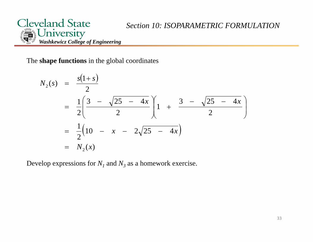
The shape functions in the global coordinates

Develop expressions for N1 and N3 as a homework exercise.

)(

42521021

24253

12

425321

21)(

2

2

xN

xx

xx

sssN

33



Graphically the shape functions for node #2 plot as follows in the two coordinate systems

N2 (x) is slightly more complicated

but is painful to use with more than one element. Think about where to place the origin of the coordinate system.

1 2

s1 1

3

N2(s)

1 2x

3

4 2 11

N2(x)

N2 (s) is a simple polynomial

2

1)(2sssN

xxxN 42521021)(2

34



Matrices for a Line Element

For a line element with quadratic shape functions

The strain displacement relationship is once again

dNuNuNuNu

332211

dB

ux

Nux

Nux

Nxu

33

22

11

35



E

Here

and stress is once again for a linear element is

x

Nx

Nx

NB 321 ,,

The only difference from before is that the shape functions are formulated in the natural coordinate system

and the derivatives above are expressed in the global x-coordinate system.

23

2

1

1)(2

1)(

21)(

ssN

sssN

sssN

36



We know that because we use an isoparametric mapping that

and we will use this expression to formulate the components of the {B} matrix which are derivatives of the shape functions. Using the chain rule from calculus

In Elasticity we derived the relationship

If J was greater than 1 we had volume expansion, between zero and 1 corresponds to volume contraction. Interpreting this relationship in terms of a line element we have

3

1)(

iii xsNx

dxds

ssN

xsN ii

)()(

dsJdx

odVJdV

37



or

From a computational standpoint

For a line element the calculation immediately above is made, inverted and used in the following expression:

Now the derivative of the shape functions are formulated in terms of the natural coordinate system.

3

1

)(i

ii x

dssdN

dsdxJ

dssdN

J

dxds

dssdN

xsN

i

ii

)(1

)()(

Jdxds 1

38



For the 3-noded line element

and the {B} matrix in the natural coordinate system is

321

3

1

22

122

12

)(

xsxsxs

xds

sdNJi

ii

sss

JB 2,

212,

2121

39



The element stiffness matrix is expressed as

The integral associated with ANY element in the global coordinates is transformed to an integral in the natural coordinate system where the integration will be from -1 to 1 in the local coordinates.

The Jacobean is a function of the s-coordinate in general and appears in the integrals. The specific form of J is determined by the values of x1, x2 and x3.

The components of the {B} matrix are polynomial functions in the s-coordinate system. In general Gaussian quadrature is used to evaluate the stiffness matrix.

Moreover, now think about the utility of the shape functions. Here their derivatives (the {B} matrix) are used to formulate the stiffness matrix in addition to their use in interpolating geometry (isoparametric elements), displacements through the elements, strains through the elements and stresses through the elements.

1

1

2

1

dsJABEB

dxABEBk

T

x

x

T

40



Gauss QuadratureIn very simple terms a definite integral is defined as

where

Attention is now given to methods that can evaluate this definite integral numerically. A characteristic of a group of numerical integration, or quadrature, techniques known as Newton-Cotes equations are that integral estimates are based on evenly spaced values of the function. Consequently, the location of the evaluation points used in these types of numerical integration method are fixed, or predetermined.

41

aFbF

dxxfIb

a

dx

xdFxf



Consider the trapezoidal rule which is the simplest method of the group. This method is based on taking the area under the straight line connecting the function values at the end of the integration interval. The formula for the trapezoidal rule is

Because the trapezoidal rule must use end point values of the function there are cases where the error associated with computation given above results in significant error. The integration error is quite noticeable with the function presented in the figure below.

42

2bfafab

dxxfIb

a

a b



Next consider that the restraint of fixed base points is relaxed and one is free to evaluate the area under the straight line joining any two points on the curve. Note that the length of the base of the trapezoid is maintained.

By positioning the two points on the curve wisely, a straight line could be positioned that would balance the positive and negative errors. This is depicted in the following figure

Gauss quadrature is the name given to one class of techniques that implement this type of strategy. Before describing the approach and its use in deriving stiffness matrices for isoparametric elements we show how numerical integration formulas such as the trapezoidal rule can be found using the method of undetermined coefficients. This method will then be used to develop the Gauss quadrature formula. 43

a b



To illustrate the method of undetermined coefficients consider an alternative formulation for the trapezoidal rule

where c0 and c1 are constants. Realizing the trapezoidal rule must yield exact results when the function being integrated is a constant, or a linear function of x, then one can use these results to generate the trapezoidal rule. Consider that for f(x) = 1

n

iii

b

a

xfcbfcafc

bfafab

dxxfI

121

2

ab

dxcc

ab

ab

2

2

21 111

44

Undetermined Coefficients



And for f(x) = x

These two integrals yield two equations for the two unknown coefficients. Solving them simultaneously yields

which when substituted back into the original formulation for the integral of the function gives us back the trapezoidal rule, i.e.,

022

2

2

21

ab

ab

dxxabcabc

221

abcc

bfafab

bfabafabbfcafcI

2

22

21

45



The objective of the Gauss quadrature approach is to determine the unknown constants for the expression

However in contrast to the trapezoidal rule that used fixed end points a and b, the function arguments x1 and x2 are not fixed and treated as unknowns. Now we need four integral expressions to find the four unknowns, c1, c2 , x1 and x2.

We obtain these conditions by assuming the equation above produces the integral value exactly for a constant function and a linear function, i.e., equality holds for

keeping in mind that

2211 xfcxfcI

1

12211

1

12211 1

dxxxfcxfc

dxxfcxfc

46

1

1

1

1

0

21

dxx

dx



We use the “canonical” form of the integrals, i.e., the limits of integration are from -1 to 1 because these are the limits of integration we will use for isoparametric elements.

To arrive at two additional conditions we assume that the Gauss quadrature formulation yields exact results when the integrand is a polynomial of degree 3 or less.

On the previous overhead geometric arguments were made to make the point that equality holds exactly. Equality for these two expressions will be demonstrated momentarily.

If the two expressions above are exact, then

1

1

32222

1

1

22211

dxxxfcxfc

dxxxfcxfc

47

2211

1

1

3

2211

1

1

2

0

32

xfcxfcdxx

xfcxfcdxx



These two expressions along with the two previous expressions yields four equations in terms of four unknowns, i.e.,

which leads to (homework assignment)

48

0

32

0

211

322

3112211

222

2112211

22112211

212211

xcxcxfcxfc

xcxcxfcxfc

xcxcxfcxfc

ccxfcxfc

5773503.03

1

5773503.03

11

2

1

21

x

x

cc



Consider the following integral with cubic polynomial integrand

Using the Gauss quadrature for this integral yields

One concludes from this brief example that the Gauss quadrature is exact for polynomials that are cubic or less. 49

1

1

32

32dxxxI

32

5773503.05773503.015773503.05773503.01 3232

32

222

31

211

2211

xxcxxc

xfcxfcI



Beyond the two point formula described previously, three, four, five and six point versions of the Gauss quadrature approach have been used. The general form is

where n is the number of quadrature points. Values of c’s and x’s are summarized in the table to the right:

n

iii

nn

xfc

xfcxfcxfcI

1

2211

50

Number of gauss points Integration location, xi Weight, ci

1 x1 = 0 c1 = 2

2 x1 = ‐ 0.57735026918962 c1 = 1

x2 = + 0.57735026918962 c2 = 1

3 x1 = ‐ 0.77459666924148 c1 = 0.555556x2 = 0 c2 = 0.888889

x3 = + 0.77459666924148 c3 = 0.555556

4 x1 = ‐ 0.861136312 c1 = 0.3478548x2 = ‐ 0.339981044 c2 = 0.6521452x3 = + 0.339981044 c3 = 0.6521452x4 = + 0.861136312 c4 = 0.3478548

5 x1 = ‐0.906179846 c1 = 0.23692695x2 = ‐ 0.538469310 c2 = 0.4786287

x3 = 0.0 c3 = 0.5688889x4 = + 0.538469310 c4 = 0.4786287

x5 = +0.906179846 c5 = 0.23692695

6 x1 = ‐0.93246914 c1 = 0.1713245x2 = ‐ 0.661209386 c2 = 0.3607616x3 = ‐0.238619186 c3 = 0.4679139x4 = + 0.238619186 c4 = 0.4679139x5 = +0.661209386 c5 = 0.3607616x6 = +0.93246914 c6 = 0.1713245



If we want to extend this approach to integration over an area, say for an isoparametric element, then

In general, we do not have to use the same number of Gauss points in each direction, i.e., idoes not have to equal j, but in finite element analysis this is typically done.

n

ijiij

n

j

n

ijii

n

jj

n

iii

tsfcc

tsfcc

dttsfc

dtdstsfI

11

11

1

1 1

1

1

1

1

,

,

,

,

51



Consider a four point Gauss integration which is shown in following figure

where for an arbitrary function of s and t

where all sampling points are +0.5773 or -0.5773 and all coefficients are equal to one. Hence the double integral is double summation technically, but really it is a single summation over four points in the element, i.e., the Gauss points.

2222121221211111

2

1

2

1

1

1

1

1

,,,,

,

,

tsfcctsfcctsfcctsfcc

tsfcc

dtdstsfI

n

ijiij

n

j

52



For a volume element we can easily extend the concepts as follows:

n

kkjikji

n

j

n

iztsfccc

dzdtdsztsfI

111

1

1

1

1

1

1

,,

,,

53



Element Stiffness MatrixIn general for a two dimensional element we have shown that

For a quadrilateral isoparametric element

If we use Gauss quadrature to evaluate the integral

A

TT dydxtBDBk

1

1

1

1

dtdstJBDBk TT

21212121

22222222

12121212

11111111

1

1

1

1

,,,

,,,

,,,

,,,

ccttsJtsBDtsB

ccttsJtsBDtsB

ccttsJtsBDtsB

ccttsJtsBDtsB

dtdstJBDBk

TTT

TTT

TTT

TTT

TT

54



In Class Example

55

F K d F K - Academic Server| Cleveland State...

Documents

Transcript of F K d F K - Academic Server| Cleveland State...