Eye movement instabilities and nystagmus canbe predicted by a nonlinear dynamics model of

the saccadic system

Akman, O. E. and Broomhead, D. S. and Abadi,R. V. and Clement, R. A.

2005

MIMS EPrint: 2006.23

Manchester Institute for Mathematical SciencesSchool of Mathematics

The University of Manchester

Reports available from: http://eprints.maths.manchester.ac.uk/And by contacting: The MIMS Secretary

School of Mathematics

The University of Manchester

Manchester, M13 9PL, UK

ISSN 1749-9097

Eye movement instabilities and nystagmus can be predicted

by a nonlinear dynamics model of the saccadic system

O.E. Akman∗

The School of Mathematics, The University of Manchester

P.O. Box 88, Manchester M60 1QD, U.K.

D.S. Broomhead

The School of Mathematics, The University of Manchester

P.O. Box 88, Manchester M60 1QD, U.K.

R.V. Abadi

Faculty of Life Sciences, Moffat Building, The University of Manchester

Sackville St, Manchester M60 1QD, U.K.

R.A. Clement

Visual Sciences Unit, Institute of Child Health, U.C.L.

30 Guilford Street, London WC1N 1EH, U.K.

Abstract

The study of eye movement control and oculomotor disorders has, for four decades,

relied on control theoretic concepts for its theoretical foundation. This paper is an

example of a complementary approach based on the theory of nonlinear dynamical

systems. Recently, a nonlinear dynamics model of the saccadic system was devel-

oped, comprising a symmetric piecewise-smooth system of six first-order autonomous

ordinary differential equations. A preliminary numerical investigation of the model

revealed that in addition to generating normal saccades, it could also simulate inaccu-

rate saccades, and the oscillatory instability known as congenital nystagmus (CN). By

varying the parameters of the model, several types of CN oscillations were produced,

including jerk, bidirectional jerk and pendular nystagmus.

The aim of this study was to investigate the bifurcations and attractors of the

model, in order to obtain a classification of the simulated oculomotor behaviours. The

application of standard stability analysis techniques, together with numerical work,

revealed that the equations have a rich bifurcation structure. In addition to Hopf,

homoclinic and saddlenode bifurcations organised by a Takens-Bogdanov point, the

equations can undergo nonsmooth pitchfork bifurcations and nonsmooth gluing bifur-

cations. Evidence was also found for the existence of Hopf-initiated canards.

∗Now at: Mathematics Institute, University of Warwick, Coventry CV4 7AL, UK

1

The simulated jerk CN waveforms were found to correspond to a pair of post-canard

symmetry-related limit cycles, which exist in regions of parameter space where the

equations are a slow-fast system. The slow and fast phases of the simulated oscillations

were attributed to the geometry of the corresponding slow manifold. The simulated

bidirectional jerk and pendular waveforms were attributed to a symmetry invariant

limit cycle produced by the gluing of the asymmetric cycles.

In contrast to control models of the oculomotor system, the bifurcation analysis

places clear restrictions on which kinds of behaviour are likely to be associated with

each other in parameter space, enabling predictions to be made regarding the possible

changes in the oscillation type that may be observed upon changing the model parame-

ters. The analysis suggests that CN is one of a range of oculomotor disorders associated

with a pathological saccadic braking signal, and that jerk and pendular nystagmus are

the most probable oscillatory instabilities. Additionally, the transition from jerk CN

to bidirectional jerk and pendular nystagmus observed experimentally when the gaze

angle or attention level is changed is attributed to a gluing bifurcation. This suggests

the possibility of manipulating the waveforms of subjects with jerk CN experimentally

to produce waveforms with an extended foveation period, thereby improving visual

resolution.

1 Introduction

Traditionally, the study of eye movement control and oculomotor disorders has been dom-

inated by control theory [35], [42], [33], [41], [30], [21]. In the last few years, however,

there has been increasing interest in the use of nonlinear dynamics techniques to model

oculomotor control, and to analyse eye movement time series [3], [37], [25], [18], [7], [20].

The oculomotor control subsystem that is responsible for the generation of fast eye move-

ments (saccades) has been the focus of much theoretical and experimental work [14], [42],

[36], [18], [24]. A recent nonlinear dynamics model of the saccadic system proposed in [18]

was found to be able to simulate normal saccades, abnormal saccades and normal saccades

with a dynamic overshoot. In that work, numerical evidence was presented to show that a

saccadic system model alone can generate both slow and fast eye movements. Indeed, the

model was found to generate waveforms resembling those associated with the pathological

oculomotor instability known as congenital nystagmus (CN), which is currently believed to

be a disorder of one or more of the oculomotor subsystems responsible for the generation

of non-saccadic eye movements [1].

This paper describes the results of a bifurcation analysis of the model, and presents

a number of implications of the analysis for understanding saccadic abnormalities and

the aetiology of CN. In section 2, a brief overview of the relevant biology is given. The

derivation of the model equations is described in section 3, where it is also argued that the

analysis of the model can effectively be reduced to that of the equations representing the

dynamics of the neurons which generate the saccadic control signal. Section 4 presents the

2

main results of the bifurcation analysis, enabling the simulated waveforms to be organised

around the corresponding bifurcation curves, and the morphology of each waveform to be

interpreted in terms of the corresponding fixed point or limit cycle attractor. The results

of section 4 are summarised in figure 15.

Lastly, the biological implications of the analysis are discussed in section 5. Chief

amongst these is the suggestion that CN may be a disorder of the saccadic system. This

view conflicts with the characterisation of CN as an abnormality of one of the oculomotor

control subsystems responsible for slow eye movement control and fixation, based on the

findings of many of the control models [33], [30], [21]. In these models, it is implicitly

assumed that the saccadic system is functioning within its normal parameter range. By

contrast, the analysis presented here implies that CN may be part of a range of disorders

produced by an abnormal saccadic braking signal. Moreover, this work challenges the

control theory explanation for the morphology of jerk CN as a slow drift from the target

generated by a slow eye movement disorder, followed by a corrective saccade to refixate the

target. The characteristic slow-fast form of jerk CN is instead attributed to the geometry

of an underlying slow manifold in the saccadic system phase space.

Several implications of this work are in agreement with previous psychophysical investi-

gations. The existence of a canard implies that once the system has developed a sustained

oscillatory instability, the oscillation is likely to be a jerk, bidirectional jerk or pendular

CN. This is consistent with the results of a recent study of oscillatory eye movement disor-

ders [2]. Additionally, the mechanism by which dynamic overshoots are generated by the

model suggest that the movements are caused by reversals of the saccadic control signal,

as predicted by a previous study of the metrics of dynamic overshoots [12].

Finally, an outcome of this work which may have clinical implications is the suggestion

that the transition from a jerk nystagmus to a bidirectional jerk nystagmus, which is often

observed experimentally, may be a consequence of a gluing bifurcation. This implies the

possibility of periodically forcing a target viewed by a jerk CN subject so as to bring

the system close to homoclinicity, producing waveforms that give rise to lower retinal slip

velocities, and hence to improved visual performance.

2 Oculomotor control, saccades and congenital nystagmus

2.1 Oculomotor control and saccades

In broad terms, the oculomotor system controls the movement of the eyes so as to ensure

that the image of the object of interest falls on the region of the retina known as the fovea

(a process referred to as foveation) [23]. Resolution of detail decreases sharply away from

the fovea and is also degraded if images slip over the fovea at velocities greater than a

few degrees per second. Consequently, optimal visual performance is only attained when

images are held steady on this region [44].

3

Saccades are fast movements of the eye which bring about foveation of new targets [43].

The oculomotor subsystem responsible for the generation of horizontal saccades behaves

in a very machine-like way. Experimental investigations of the dynamic characteristics of

saccades have revealed that the peak velocity and duration of a saccade are related to its

amplitude [43], [17]. This relationship is often referred to as the main sequence, and is

used to classify an eye movement as a saccade [13].

A recording of a simple accurate (normometric) saccade is shown in figure 1-A. Normometric

saccades often have a post-saccadic component referred to as a dynamic overshoot [34], [7].

A recorded dynamic overshoot is shown in figure 1-B. Inaccurate or dysmetric saccades

can take the form of an initial undershoot (hypometric saccade) or overshoot (hypermetric

saccade) of the desired eye position, resulting in a secondary corrective saccade [14].

Neurophysiological studies have shown that the saccadic control signal for horizontal

saccades is generated by excitatory burst neurons in the brainstem. These are normally

inhibited by omnipause neurons, except during a saccade, when the omnipause neurons

cease firing. The firing rate of a burst neuron is a saturating nonlinear function of the

dynamic motor error m, which is the difference between the required and current eye

positions [42]. The burst neurons are divided into two types: right burst neurons which

fire maximally for rightward saccades and left burst neurons which fire maximally for

leftward saccades. The overall burst signal b can be expressed as the difference between

the signals r and l from the right and left burst neurons respectively.

In addition to the response in the direction of maximal firing (the on-response), the

burst neurons also have a small response in the opposite direction (the off-response). The

off-response is believed to correspond to a small centripetal tug at the end of a small-

amplitude movement that prevents the inertia of the eye causing overshoot of the target

[42]. This will be referred to here as a braking signal. The effectiveness of the braking

signal in slowing the eye at the end of the movement increases with the magnitude of the

off-response. Evidence has also been found suggesting that burst neurons exhibit mutual

inhibition, with the firing of right burst neurons suppressing that of left burst neurons, and

vice versa [39].

According to the displacement feedback model of saccade generation illustrated in figure

2, saccades are produced in response to a desired gaze displacement signal ∆g generated by

higher brain centres [36]. In this scheme, the motor error m is obtained by subtracting an

estimate s of current eye displacement from ∆g. The burst signal b is sent to a complex of

neurons in the brain stem, the neural integrator, which integrate it. The integrated signal

n is then added to b, and the summed signal is relayed to the relevant ocular motoneurons.

These send the final motor command to the eye muscles, which produce a shift in the eye

position g. A copy of b is sent to a separate resettable integrator to generate the estimate s.

The epithet ‘resettable’ refers to the fact that s is required to be set to 0 at the beginning

of each saccade. This feedback model should act so as to drive m to 0, moving the eye to

4

0 0.1 0.2 0.3−2

0

2

4

6

8

10

12

14A

g(t)

(de

gs)

0 0.1 0.2 0.3 0.4 0.5−2

0

2

4

6

8

10

12

14B

0 0.2 0.4 0.6 0.8 1−2

−1.5

−1

−0.5

0

0.5C

0 0.2 0.4 0.6 0.8−4

−3

−2

−1

0

1

2

3D

0 0.2 0.4 0.6 0.8 1−8

−6

−4

−2

0

2

4E

0 0.2 0.4 0.6 0.8 10.6

0.8

1

1.2

1.4

1.6

1.8F

t (secs)

Figure 1: Recorded eye movements. t=time, g(t)=horizontal eye position, with g(t) > 0

corresponding to rightward gaze. A: normometric saccade. B: dynamic overshoot. C:

left-beating jerk CN. D: jerk with extended foveation. E: bidirectional jerk. F: pendular

CN. In A and B, the dotted line indicates the target position.

5

BURST NEURONS

NEURAL INTEGRATOR

MUSCLE PLANT

RESETTABLE INTEGRATOR

∆g

s

m b-+

n g

Figure 2: The displacement feedback model of saccade generation. A copy of the burst

signal b is integrated to obtain an estimate of current eye displacement s which is fed back

to generate the motor error m. g and n denote the gaze angle and integrated burst signal

respectively. ∆g denotes the required gaze displacement signal generated by higher brain

centres, which initiates the saccade.

the required position g (0) + ∆g. In control models of the oculomotor system, the ocular

motoneurons and eye muscles are referred to collectively as the muscle plant.

2.2 Congenital nystagmus

CN is an involuntary, bilateral oscillation of the eyes that is present in approximately 1 in

4000 of the population [4]. The oscillations in each eye are strongly correlated, and occur

primarily in the horizontal plane. In general, the retinal image is held on the fovea for

a short time before a slow phase takes the target off the fovea. The slow phase is then

interrupted by a fast or slow phase which moves the target directly onto the fovea [22], [4],

[5]. As a consequence of the reduced foveation time, CN subjects tend to have poor visual

acuity [6], [9], [16]. Some recordings of common CN waveforms are shown in figure 1. Jerk

CN consists of an increasing exponential slow phase followed by a saccadic fast phase (fig.

1-C). The direction of the fast phase is referred to as the beat direction. Two variations

on jerk are jerk with extended foveation, in which the eye spends a greater time in the

vicinity of the foveation position (fig. 1-D), and bidirectional jerk, in which the eye beats

alternately in both directions (fig. 1-E). The less common pendular nystagmus consists of

sinusoidal slow phase movements (fig. 1-F).

Most CN subjects exhibit a range of different oscillations over a single recording period,

with the particular waveform observed depending on factors such as gaze angle, attention

and stress. In particular, it has been found that some subjects who exhibit a jerk nystagmus

during a fixation task can switch to a pendular nystagmus upon entering a state of low

attention, such as when closing their eyes or daydreaming [4], [5]. Many CN subjects

have a gaze angle referred to as the neutral zone, in which the beat direction changes.

Bidirectional oscillations can be observed close to the neutral zone [4].

6

3 A nonlinear dynamics model of the saccadic system

3.1 The model

The displacement feedback model of figure 2 can be described using the set of coupled

ODEs below [18]:

g = v (1)

v = −(

1

T1+

1

T2

)

v − 1

T1T2g +

1

T1T2n+

(

1

T1+

1

T2

)

(r − l) (2)

n = − 1

TNn+ (r − l) (3)

r =1

ǫ

(

−r − γrl2 + F (m))

(4)

l =1

ǫ

(

−l − γlr2 + F (−m))

(5)

m = − (r − l) . (6)

Equations (1) and (2) model the response of the muscle plant to the signals generated

by the burst neurons. Here, g represents the eye position and v the eye velocity. These

equations are based on quantitative investigations of physical eye movements which show

that the muscle plant can be modelled as a second-order linear system with a slow time

constant T1 = 0.15s and a fast time constant T2 = 0.012s [33]. (3) is the equation for n,

the signal from the neural integrator. The slow time constant TN = 25s corresponds to

the slow post-saccadic drift back to zero degrees observed experimentally [15].

(4) and (5) are the equations for the activities r and l of the right and left burst neurons.

The function F (m) defined by

F (m) =

α′(

1 − e−m/β′

)

if m ≥ 0

−αβme

m/β if m < 0(7)

models the response of the burst neurons to the motor error signal m. The form of F (m)

is based on the results of single-cell recordings from alert monkeys [42]. A schematic plot

of F (m) is shown in figure 3.

The function has four positive parameters, α′, β′, α and β which govern the forms of the

modelled on- and off- responses. For m ≥ 0, F (m) is increasing, with F (m) → α′ as m→∞. Also, F (β′) = α′

(

1 − e−1)

. α′ therefore determines the value at which the modelled

on-response saturates as m → ∞, and β′ determines how quickly the saturation occurs.

For m < 0, F (m) has a single global maximum at(

−β, αe

)

, and converges monotonically

to 0 as m→ −∞ from −β. α thus determines the magnitude of the modelled off-response,

and hence the strength of the corresponding braking signal. β determines the motor error

range over which a significant off-response occurs, and therefore the range for which there

is effective braking.

7

F(m

)

α′

β′−β

αe−1

m

α′(1−e−1)

Figure 3: Schematic of the function F (m) used to model the response curve for a saccadic

burst neuron. The parameters α′ and β′ determine the modelled on-response while α and

β determine the modelled off-response.

The terms γrl2 and γlr2 represent the mutual inhibition between the left and right

burst neurons, with the parameter γ determining the strength of the inhibition. ǫ is a

parameter which determines how quickly the neurons respond to the motor error signal m

with the response time decreasing as ǫ is decreased. (6) is the equation for the resettable

integrator, obtained by substituting m = ∆g − s into s = b. Note that it is assumed that

the resettable integrator is a perfect integrator, in contrast to the neural integrator which

is leaky.

The parameters α′, β′ and γ are fixed at α′ = 600, β′ = 9 and γ = 0.05, on the basis

that these values give simulated saccades which lie on the main sequence [18]. The variable

parameters of the model are thus α, β and ǫ, representing the off-response magnitude, off-

response range and burst neuron response time respectively.

It should be noted that although the omnipause neurons are not explicitly included in

the model, the burst neuron response function F (m) implicitly incorporates the effects of

both the burst neurons and the omnipause neurons. The omnipause neurons are active

during the end of a saccade when they fire in order to bring the saccade to a stop, and

therefore contribute to the form of F (m) about m = 0.

3.2 Characterisation of the model as a skew-product

By setting x = (g, v, n)T and y = (r, l,m)T , the system can be written in the skew-product

form

x = Ax +By

y = G (y) ,

8

where A and B are the constant matrices

A =

0 1 0

− 1T1T2

−(

1T1

+ 1T2

)

1T1T2

0 0 − 1TN

, B =

0 0 01T1

+ 1T2

−(

1T1

+ 1T2

)

0

1 −1 0

,

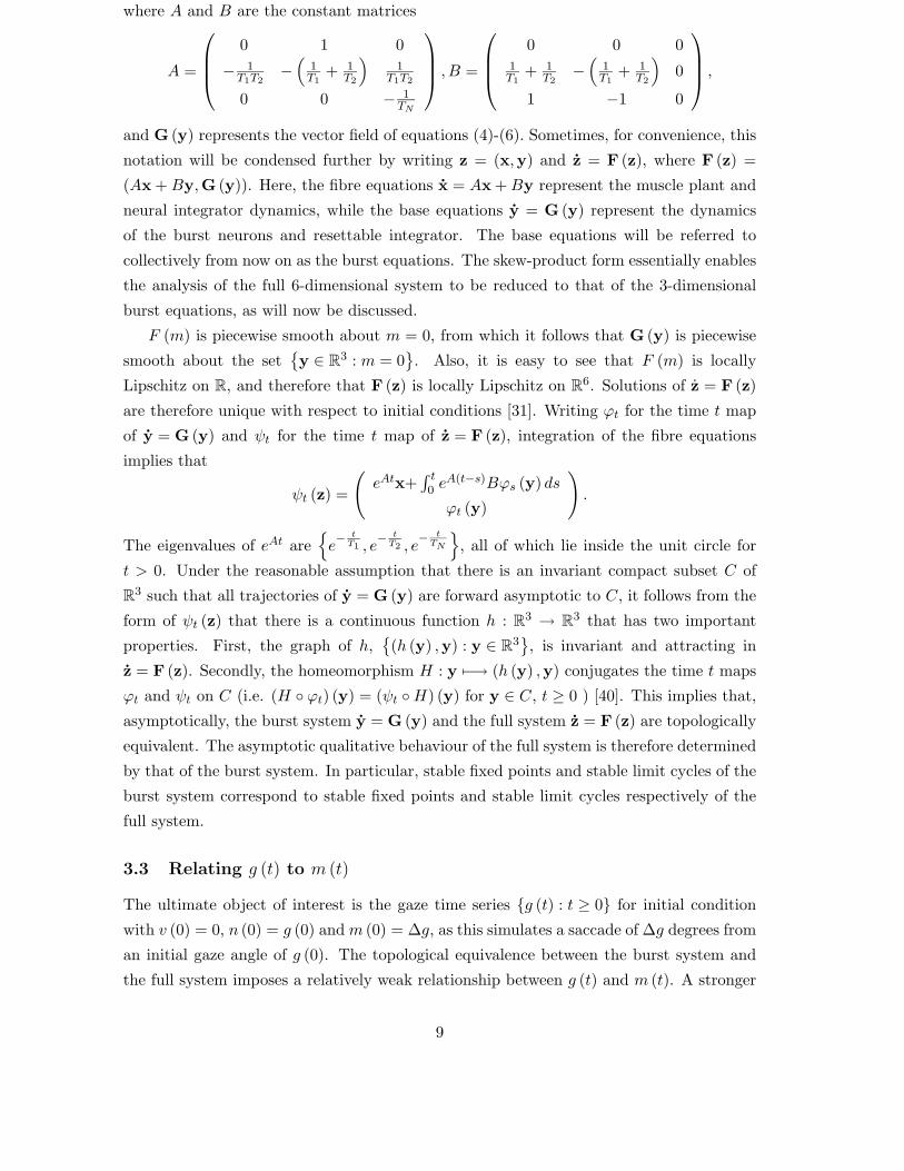
and G (y) represents the vector field of equations (4)-(6). Sometimes, for convenience, this

notation will be condensed further by writing z = (x,y) and z = F (z), where F (z) =

(Ax +By,G (y)). Here, the fibre equations x = Ax +By represent the muscle plant and

neural integrator dynamics, while the base equations y = G (y) represent the dynamics

of the burst neurons and resettable integrator. The base equations will be referred to

collectively from now on as the burst equations. The skew-product form essentially enables

the analysis of the full 6-dimensional system to be reduced to that of the 3-dimensional

burst equations, as will now be discussed.

F (m) is piecewise smooth about m = 0, from which it follows that G (y) is piecewise

smooth about the set{

y ∈ R3 : m = 0

}

. Also, it is easy to see that F (m) is locally

Lipschitz on R, and therefore that F (z) is locally Lipschitz on R6. Solutions of z = F (z)

are therefore unique with respect to initial conditions [31]. Writing ϕt for the time t map

of y = G (y) and ψt for the time t map of z = F (z), integration of the fibre equations

implies that

ψt (z) =

(

eAtx+∫ t0 e

A(t−s)Bϕs (y) ds

ϕt (y)

)

.

The eigenvalues of eAt are{

e− t

T1 , e− t

T2 , e− t

TN

}

, all of which lie inside the unit circle for

t > 0. Under the reasonable assumption that there is an invariant compact subset C of

R3 such that all trajectories of y = G (y) are forward asymptotic to C, it follows from the

form of ψt (z) that there is a continuous function h : R3 → R

3 that has two important

properties. First, the graph of h,{

(h (y) ,y) : y ∈ R3}

, is invariant and attracting in

z = F (z). Secondly, the homeomorphism H : y 7−→ (h (y) ,y) conjugates the time t maps

ϕt and ψt on C (i.e. (H ◦ ϕt) (y) = (ψt ◦H) (y) for y ∈ C, t ≥ 0 ) [40]. This implies that,

asymptotically, the burst system y = G (y) and the full system z = F (z) are topologically

equivalent. The asymptotic qualitative behaviour of the full system is therefore determined

by that of the burst system. In particular, stable fixed points and stable limit cycles of the

burst system correspond to stable fixed points and stable limit cycles respectively of the

full system.

3.3 Relating g (t) to m (t)

The ultimate object of interest is the gaze time series {g (t) : t ≥ 0} for initial condition

with v (0) = 0, n (0) = g (0) and m (0) = ∆g, as this simulates a saccade of ∆g degrees from

an initial gaze angle of g (0). The topological equivalence between the burst system and

the full system imposes a relatively weak relationship between g (t) and m (t). A stronger

9

relationship can be obtained by utilising the linearity of the fibre equations in x, enabling

the morphology of g (t) to be inferred from that of m (t), when the attractors of the model

are fixed points or limit cycles. This in turn allows the form of the simulated eye movement

to be related directly to the corresponding attractor of the burst equations in these cases.

Introducing Laplace transforms and the specified initial conditions it is possible to show

that

g (t) = g (0)R (t) + (g (0) + ∆g)S (t) + (ug ∗m) (t) , (8)

where

R (t) =1

T1 − T2

(

T1e− t

T2 − T2e− t

T1

)

(9)

S (t) = K1T1e− t

T1 +K2T2e− t

T2 +KNTNe− t

TN (10)

ug (t) = K1e− t

T1 +K2e− t

T2 +KNe− t

TN , (11)

with the constants K1, K2, KN given by

K1 =T 2

1 + T2 (T1 − TN )

T1 (T1 − T2) (T1 − TN )

K2 =T1 (TN − T2) − T 2

2

T2 (T1 − T2) (T2 − TN )

KN =T 2

N

TN (T1 − TN ) (T2 − TN ).

In terms of the response function

Tg (s) =−s((

1T1

+ 1T2

)

s+(

1T1TN

+ 1T2TN

+ 1T1T2

))

(

s+ 1T1

)(

s+ 1T2

)(

s+ 1TN

) (12)

of the linear system (8), S (t) and ug (t) can be written succinctly as:

S (t) = L−1

[

−Tg (s)

s

]

(13)

ug (t) = L−1 [Tg (s)] . (14)

(In the above expressions, ∗ represents Laplace convolution while L−1 denotes the inverse

Laplace transform).

In practise, there are simple approximations to these quantities which are valid for

physiologically realistic values of the parameters. Using the known values of T1, T2 and

TN gives

|T2 (T1 − TN )| ≫ T 21

|T1 (TN − T2)| ≫ T 22

TN ≫ T1, T2,

10

0 0.2 0.4 0.6 0.8 10

0.2

0.4

0.6

0.8

1

1.2

t

S(t

)

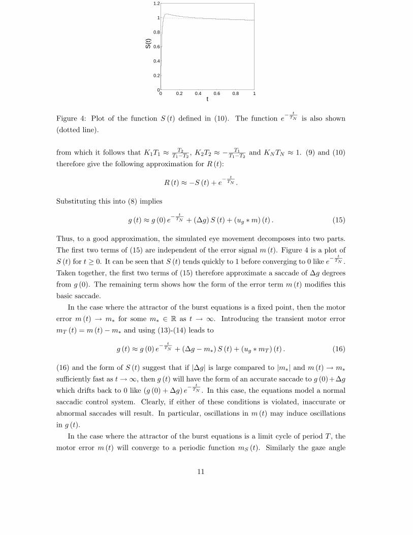
Figure 4: Plot of the function S (t) defined in (10). The function e− t

TN is also shown

(dotted line).

from which it follows that K1T1 ≈ T2

T1−T2, K2T2 ≈ − T1

T1−T2and KNTN ≈ 1. (9) and (10)

therefore give the following approximation for R (t):

R (t) ≈ −S (t) + e− t

TN .

Substituting this into (8) implies

g (t) ≈ g (0) e− t

TN + (∆g)S (t) + (ug ∗m) (t) . (15)

Thus, to a good approximation, the simulated eye movement decomposes into two parts.

The first two terms of (15) are independent of the error signal m (t). Figure 4 is a plot of

S (t) for t ≥ 0. It can be seen that S (t) tends quickly to 1 before converging to 0 like e− t

TN .

Taken together, the first two terms of (15) therefore approximate a saccade of ∆g degrees

from g (0). The remaining term shows how the form of the error term m (t) modifies this

basic saccade.

In the case where the attractor of the burst equations is a fixed point, then the motor

error m (t) → m∗ for some m∗ ∈ R as t → ∞. Introducing the transient motor error

mT (t) = m (t) −m∗ and using (13)-(14) leads to

g (t) ≈ g (0) e− t

TN + (∆g −m∗)S (t) + (ug ∗mT ) (t) . (16)

(16) and the form of S (t) suggest that if |∆g| is large compared to |m∗| and m (t) → m∗

sufficiently fast as t→ ∞, then g (t) will have the form of an accurate saccade to g (0)+∆g

which drifts back to 0 like (g (0) + ∆g) e− t

TN . In this case, the equations model a normal

saccadic control system. Clearly, if either of these conditions is violated, inaccurate or

abnormal saccades will result. In particular, oscillations in m (t) may induce oscillations

in g (t).

In the case where the attractor of the burst equations is a limit cycle of period T , the

motor error m (t) will converge to a periodic function mS (t). Similarly the gaze angle

11

0 20 40 60 80 1000

0.2

0.4

0.6

0.8

1

1.2

1.4

ωA

(ω)

0 20 40 60 80 1002

2.5

3

3.5

ω

φ(ω

)

Figure 5: Plots of the amplitude variable A (ω) and phase variable φ (ω) of the linear filter

Tg (iω) defined in (12) on the range (0, 100).

g (t) will converge to a periodic function gS (t) which (because of the linearity of the fibre

dynamics) also has period T . Moreover, writing mS (t) as the Fourier series

mS (t) =∞∑

k=−∞

mSk e

ikωT t

where ωT = 2πT , ignoring transients and using the linearity of the convolution implies that

gS (t) has the Fourier series

gS (t) =∞∑

k=−∞

Tg (ikωT )mSk e

ikωT t

[32]. This is, in effect, a linear filtering of the time series {mS (t) : t ≥ 0}, where Tg (iω) is

the response function of the filter.

It is useful to write Tg (iω) in terms of amplitude and phase variables, Tg (iω) =

A (ω) eφ(ω)i. Explicit expressions for A (ω) and φ (ω) in terms of the time constants T1, T2

and TN can be obtained, but these are rather uninformative. Figure 5 shows plots of nu-

merical evaluations of A (ω) and φ (ω) for 0 < ω < 100. It is clear that A (ω) depends rather

weakly on frequency in this range. Indeed, if ω is restricted to the interval 0.08 < ω < 55,

then |A (ω) − 1| < 0.1. In the same frequency range, the phase varies approximately lin-

early. A linear regression of φ(ω) over this range implies that φ (ω) ≈ −tgω + π, where

tg = 0.0115. Taken together, these expressions for the amplitude and phase suggest the

approximation Tg (iω) ≈ −e−tgωi for 0.08 < ω < 55.

If it is assumed that the periodic functionmS (t)−〈mS (t)〉 (where 〈mS (t)〉 = 1T

∫ T0 mS (t) dt)

does not have significant energy outside the frequency range 0.08 < ω < 55, then setting

WS = {k ∈ Z : 0.08 < |kωT | < 55} gives the approximation

mS (t) − 〈mS (t)〉 ≈∑

k∈WS

mSk e

ikωT t. (17)

As |Tg (iω)| ≈ 1 for ω ∈ (0.08, 55) and |Tg (iω)| < 1 for ω /∈ (0.08, 55) with Tg (0) = 0,

it follows that gS (t) will also not have significant energy outside the frequency range

12

0.08 < ω < 55. This leads to the approximation

gS (t) ≈∑

k∈WS

Tg (ikωT )mSk e

ikωT t.

Substituting Tg (iω) ≈ −e−tgωi into the above then gives

gS (t) ≈ −∑

k∈WS

mSk e

ikωT (t−tg).

Using (17) leads to the final approximation

gS (t) ≈ −mS (t− tg) + 〈mS (t)〉 . (18)

Given this final approximation, g (t) has the form of a saccade which decays to the periodic

oscillation gS (t) as t→ ∞, where the morphology of gS (t) is determined by that of mS (t).

The equations therefore model a pathological saccadic system with an asymptotically pe-

riodic oscillatory instability, the form of which is determined by that of the corresponding

periodic motor error time series.

4 Analysis of the burst equations

It has been established in the previous sections that the asymptotic qualitative dynamics

- and even quantitative dynamics - of the full model are determined by that of the burst

equations y = G (y) given explicitly by

r =1

ǫ

(

−r − γrl2 + F (m))

(19)

l =1

ǫ

(

−l − γlr2 + F (−m))

(20)

m = − (r − l) , (21)

where F (m) = F (m;α, β) is defined in (7). Before the bifurcation analysis of the burst

equations is presented in 4.2, some general properties of the equations which aid their

analysis - such as the existence of a symmetry - are discussed

4.1 General properties of the burst equations

4.1.1 Symmetry

The vector field G (y) is equivariant under the action of the group Z2 = {id, σ}, where σ

acts linearly on R3 according to σ : (r, l,m) 7−→ (l, r,−m). If follows that σ maps trajecto-

ries of y = G (y) into each other, and that the set L0 defined by L0 ={

y ∈ R3 : σy = y

}

is invariant under the dynamics [27]. L0 is given explicitly by

L0 ={

(x, x, 0)T : x ∈ R

}

.

13

m m

F(m)

F(−m)

m2 m

1 0

F(m)

F(−m)

m1 0

A B

Figure 6: Schematic of the possible intersections of the functions F (m) and F (−m) on

the positive real line.

Restricting the vector field to L0 gives the following first order system:

x = −(

1 + γx2)

x. (22)

The point x = 0, the unique attracting fixed point of (22), corresponds to a fixed point at

the origin 0 = (0, 0, 0)T of the full system. The invariance of L0 therefore implies that it

is a 1-dimensional stable manifold of the origin. Since this property is a consequence of

the symmetry, the existence and form of this stable manifold do not depend on the model

parameters α, β and ǫ.

4.1.2 Fixed points

The existence of the symmetry σ implies that invariant sets of the equations are either

symmetry invariant, or form pairs related by the action of σ. In particular, fixed points of

(19)-(21) have the form (r∗, r∗,±m∗)T , where m∗ - which will be taken to be nonnegative

- solves F (m) = F (−m), and r∗ ≥ 0 is the unique real solution to γr3 + r − F (m∗) = 0.

Consideration of the form of F (m) shows that 0 is always a solution of F (m) = F (−m)

which gives rise to the fixed point at the origin. Nontrivial solutions of F (m) = F (−m)

on R+ can occur generically in one of two ways depending on the shape of the function

F (m), as illustrated in figure 6.

Much of this can be understood in terms of the right and left derivatives of F (m) at

m = 0. Write Λ+ for limm→0+DF (m) = α′

β′ and Λ− for limm→0−DF (m) = −αβ . Then as

suggested by figure 6-A, for α > Λ+β (that is for −Λ− > Λ+), there is a single nontrivial

solution m1 of F (m) = F (−m) on R+. For α < Λ+β (that is for −Λ− < Λ+), there are

two possibilities. For some values of β, F (m) can intersect F (−m) tangentially as α is

increased from 0 in this range. For such β values, there is a critical value of α at which the

tangency occurs; this will be written as T (β). It then follows that there are no nontrivial

solutions of F (m) = F (−m) on R+ for α < T (β), a single solution m1 for α = T (β),

and a pair of nontrivial solutions {m1,m2} for T (β) < α < Λ+β (see figure 6-B). The

convention will be that m1 and m2 are labelled so that m2 < m1. For β values such that

14

α′e

α=Λ+β

2β′

2α′α=T(β)

0

β

α

0, y1+, y

1− 0, y

1+, y

1−, y

2+, y

2−

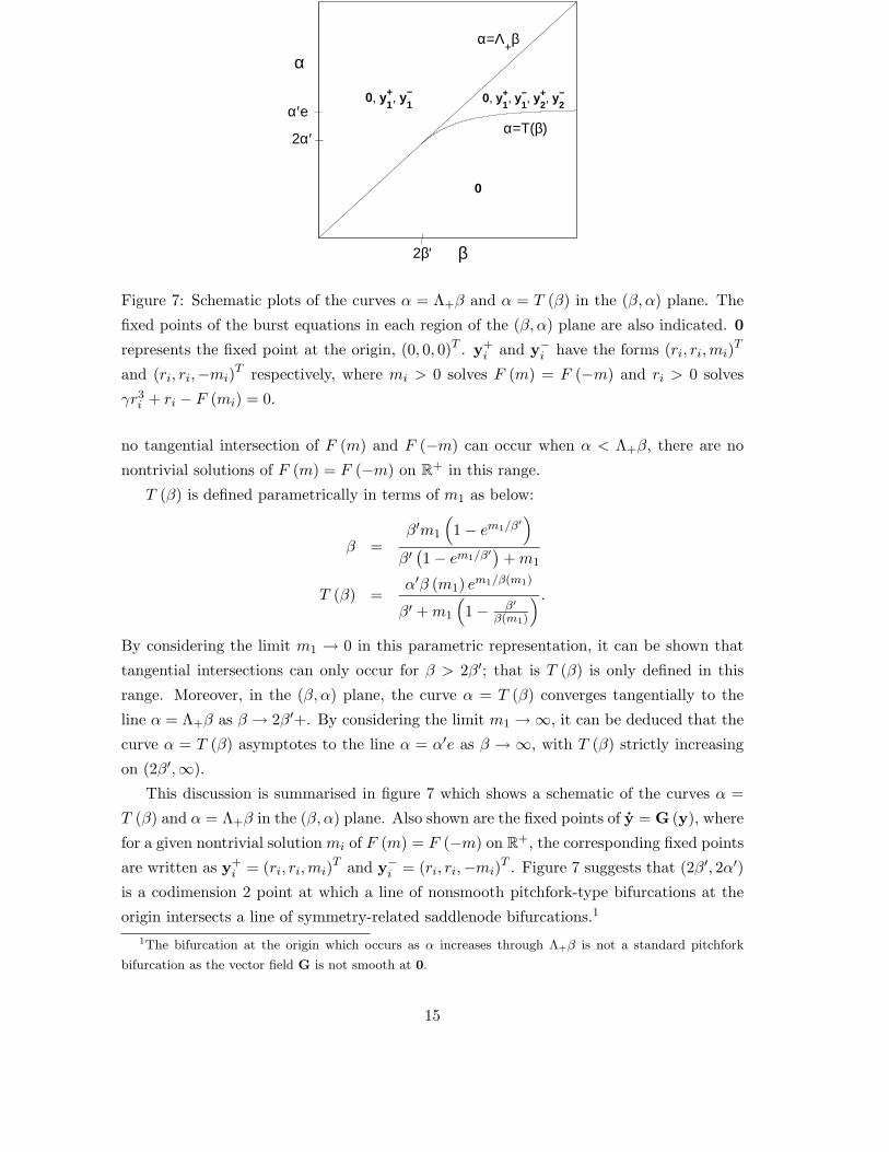
Figure 7: Schematic plots of the curves α = Λ+β and α = T (β) in the (β, α) plane. The

fixed points of the burst equations in each region of the (β, α) plane are also indicated. 0

represents the fixed point at the origin, (0, 0, 0)T . y+i and y−

i have the forms (ri, ri,mi)T

and (ri, ri,−mi)T respectively, where mi > 0 solves F (m) = F (−m) and ri > 0 solves

γr3i + ri − F (mi) = 0.

no tangential intersection of F (m) and F (−m) can occur when α < Λ+β, there are no

nontrivial solutions of F (m) = F (−m) on R+ in this range.

T (β) is defined parametrically in terms of m1 as below:

β =β′m1

(

1 − em1/β′

)

β′(

1 − em1/β′)

+m1

T (β) =α′β (m1) e

m1/β(m1)

β′ +m1

(

1 − β′

β(m1)

) .

By considering the limit m1 → 0 in this parametric representation, it can be shown that

tangential intersections can only occur for β > 2β′; that is T (β) is only defined in this

range. Moreover, in the (β, α) plane, the curve α = T (β) converges tangentially to the

line α = Λ+β as β → 2β′+. By considering the limit m1 → ∞, it can be deduced that the

curve α = T (β) asymptotes to the line α = α′e as β → ∞, with T (β) strictly increasing

on (2β′,∞).

This discussion is summarised in figure 7 which shows a schematic of the curves α =

T (β) and α = Λ+β in the (β, α) plane. Also shown are the fixed points of y = G (y), where

for a given nontrivial solution mi of F (m) = F (−m) on R+, the corresponding fixed points

are written as y+i = (ri, ri,mi)

T and y−i = (ri, ri,−mi)

T . Figure 7 suggests that (2β′, 2α′)

is a codimension 2 point at which a line of nonsmooth pitchfork-type bifurcations at the

origin intersects a line of symmetry-related saddlenode bifurcations.1

1The bifurcation at the origin which occurs as α increases through Λ+β is not a standard pitchfork

bifurcation as the vector field G is not smooth at 0.

15

4.1.3 Slow manifold

For small ǫ, the burst equations are a slow-fast system [46]. The associated slow manifold,

which will be written SM , is the union of curves given by the intersection of the r- and l-

nullclines. Trajectories contract onto SM parallel to the (r, l) plane and then evolve on SM

according to the equation m = − (r − l). Trajectories on SM therefore move along it in the

positive m direction for r < l and in the negative m direction for r > l. As ǫ is decreased,

trajectories contract onto the slow manifold more quickly and follow it more closely. It can

be seen from (19)-(20) that SM is independent of ǫ, and is invariant under σ.

A more detailed understanding of the geometric form of SM can be obtained by con-

sidering its parameterised form{

(

F (m)

1 + γlM (m)2, lM (m) ,m

)T

: m ∈ R

}

, (23)

where lM (m) solves GM (l;m) = 0, with GM (l;m) given by

GM (l;m) = l5 − F (−m) l4 +2

γl3 − 2F (−m)

γl2 +

1

γ

(

F (m)2 +1

γ

)

l − F (−m)

γ2.

Consider foliating the phase space with planes of constant m. For a given value m′ of m,

since GM (l;m) is a quintic polynomial in l, SM intersects the plane m = m′ generically

at 1, 3 or 5 points. Moreover, there is always at least one point of intersection. It follows

that in (r, l,m) space, SM always contains at least one curve, which will be written as

S1. As m is varied, new points of intersection are generated through the quintic GM (l;m)

developing pairs of additional roots.

Something of the structure of SM can be understood by considering various limits of

m. As m → 0, F (m) → 0, and so GM (l;m) → l(

l2 + 1γ

)2. This function has only one

real root at l = 0, and (23) implies that this root corresponds to the origin 0, which always

lies on SM . It follows that for small |m|, SM = S1 with S1 → 0 as m→ 0.

Considering the limit as m → ∞, F (m) → α′ and F (−m) → 0, from which it follows

that GM (l;m) → l(

l4 + 2γ l

2 + 1γ

(

(α′)2 + 1γ

))

. Again, l = 0 is the only real root of this

function implying that SM = S1 for m > 0 with m large. Moreover, (23) implies that S1

converges to the curve{

(F (m) , 0,m)T : m > 0}

as m → ∞. By symmetry, SM = S1 for

m < 0 with |m| large. Indeed, S1 converges to the curve{

(0, F (−m) ,m)T : m < 0}

as

m→ −∞, .

For intermediate values of |m|, S1 may have turning points with respect to the m axis,

while SM may contain other curves in addition to S1. As roots of GM (l;m) are created in

pairs, any such additional curves will be closed loops. Examples of the form of SM appear

in figures 9, 12 and 14.

The existence of SM restricts the behaviour of the burst equations for small ǫ. Firstly,

since all attractors must have portions lying on SM , and SM is a 1-dimensional set, it is

reasonable to assume that the only possible attractors are stable fixed points and stable

16

limit cycles. Secondly, trajectories cannot cross the m = 0 plane. This can be seen by

noting that SM = S1 for |m| small; any trajectory which crosses the plane must therefore

do so on S1, which cannot happen as S1 contains a fixed point at the origin.

4.1.4 Smooth vector fields

In interpreting the bifurcations and local dynamics of the burst equations at the origin 0

where the vector field G is not smooth, it will be useful to consider the smooth vector

fields G+ and G− defined as follows:

G+ (r, l,m) =

1ǫ

(

−r − γrl2 + α′(

1 − e−m/β′

))

1ǫ

(

−l − γlr2 + αβme

−m/β)

−(r − l)

(24)

G− (r, l,m) =

1ǫ

(

−r − γrl2 − αβme

m/β)

1ǫ

(

−l − γlr2 + α′(

1 − em/β′

))

−(r − l)

. (25)

These vector fields have been chosen so as to agree with G on the appropriate half-spaces:

G+|m≥0 = G|m≥0 and G−|m≤0 = G|m≤0. Consequently, each trajectory of y = G (y) can

be expressed as a union of sections of trajectories of y = G+(y) and y = G−(y). Also,

σ ◦ G+ = G− ◦ σ, and so solutions of y = G+(y) and y = G−(y) map into each other

under σ. As G±|m=0 = G|m=0, 0 is a fixed point of both smooth systems and L0 is a

stable manifold of 0, for all parameter values.

4.2 Bifurcations, attractors and simulated eye movements

The bifurcation analysis presented in this section is divided into two main parts. In 4.2.1,

the bifurcations of the burst equations which occur as α and β are varied for a fixed small

ǫ are described. These results provide the basis for 4.2.2, in which the restriction to small

ǫ is lifted, and the bifurcations which occur in the reduced range 1.5 < β < 6, α < α′

are considered. This reduced range contains the parameter values for which biologically

realistic simulated eye movements were found during the initial numerical investigation of

the full model presented in [18]. In 4.2.2, the morphology of each of these simulated eye

movements is interpreted in terms of the corresponding attractor of the burst equations.

The results of the section are summarised in figure 15.

4.2.1 Bifurcations and attractors for small ǫ

Figure 8 is a schematic diagram of the bifurcations and attractors of the burst equations

for small ǫ. The figure was obtained by combining standard linear stability analysis with

numerical work and the assumption that the equations have only fixed point and limit cycle

17

2β′

α=T(β)

βT

α=αH(β)

β

α

α=Λ+β

αT

0

α=H(β,∈)

0

y1+, y

1−

0, y

1+, y

1−

0

C+, C

−

0, C+, C

−

α=αC(β,∈)

2α′

βC(∈)

Figure 8: Bifurcations and attractors of the burst equations (4)-(6) for small ǫ. α = Λ+β

is a line of nonsmooth pitchfork bifurcations at the origin 0 = (0, 0, 0)T . The bifurcation is

supercritical for β < 2β′, producing a pair of stable fixed points{

y+1 ,y

−1

}

, and subcritical

for β > 2β′, destroying a pair of unstable fixed points{

y+2 ,y

−2

}

. α = T (β) is a line of

symmetry-related saddlenode bifurcations. All fixed points{

y+1 ,y

−1 ,y

+2 ,y

−2

}

produced by

the bifurcations are unstable for β > βT , while for β < βT ,{

y+1 ,y

−1

}

are created stable and{

y+2 ,y

−2

}

are created unstable. α = αH (β) is a line of symmetry-related supercritical Hopf

bifurcations at y+1 and y−

1 at which a pair of stable limit cycles {C+, C−} are produced.

α = H (β, ǫ) is a curve of symmetry-related saddlenode homoclinic bifurcations at y+2 and

y−2 which destroy C+ and C−. α = αC (β, ǫ) is a line of symmetry-related Hopf-initiated

canards at which C+ and C− undergo a sudden increase in amplitude.

18

attractors for small ǫ.2 The bifurcations are organised by a pair of codimension-two points.

The first of these is the point (2β′, 2α′) identified in section 4.1.2. The second codimension-

two point, labelled (βT , αT ), is of the Takens-Bogdanov type. Each is discussed in turn

below.

The codimension-two point (2β′, 2α′): At this point, a line α = T (β) of symmetry-

related saddlenode bifurcations intersects a line α = Λ+β of nonsmooth, pitchfork-type

bifurcations involving the origin 0. For β > βT , all fixed points{

y+1 ,y

−1 ,y

+2 ,y

−2

}

created

by the saddlenode bifurcations are unstable, while for β < βT ,{

y+1 ,y

−1

}

are created stable

and{

y+2 ,y

−2

}

are created unstable (cf. figure 7). The pitchfork-type bifurcation can occur

in two ways, depending on the sign of β−2β′. For β < 2β′, the bifurcation is supercritical:

as α increases through Λ+β, 0 loses stability and a pair of stable fixed points{

y+1 ,y

−1

}

is

created. For β > 2β′, the bifurcation is subcritical: as α increases through Λ+β, 0 loses

stability and a pair of unstable fixed points{

y+2 ,y

−2

}

is destroyed (cf. figure 7 again).

The pitchfork-type bifurcation can be understood in terms of standard transcritical and

pitchfork bifurcations which occur in the smooth system y = G+(y) defined in (24). It

can be shown that given a fixed β and ǫ, for α with |α− Λ+β| sufficiently small, the origin

has a smooth, 1-dimensional, attracting local centre manifold W+C , which is tangential to

the vector (Λ+,Λ+, 1)T at 0 when α = Λ+β. Moreover, the dynamics on W+C is given by

z = P (z, α) = (α− Λ+β) z − Λ+az2 − Λ+

(

2ǫΛ+a2 + b

)

z3 + O (3) , (26)

where

z = −ǫr + ǫl +m (27)

a =1

β− 1

2β′(28)

b =1

6 (β′)2− 1

2β2, (29)

and O (3) represents all terms of the form{

zi (α− Λ+β)j : i+ j ≥ 3}

, excluding z3 [10]. It

then follows from the symmetry that for small ǫ, the setWC defined byWC =(

W+C ∩ {y : m ≥ 0}

)

∪((

σW+C

)

∩ {y : m ≤ 0})

is a 1-dimensional, attracting local set of the piecewise smooth

system y = G (y) containing 0, on which the dynamics is given by

z = Q (z, α) =

{

P (z, α) if z ≥ 0

−P (−z, α) if z ≤ 0. (30)

A fixed point z∗ ≥ 0 of the W+C dynamics z = P (z, α) gives rise to a pair of fixed points

{z∗,−z∗} of the WC dynamics z = Q (z, α). These in turn correspond to a pair of fixed

2Many of the bifurcation curves lie very close to each other in the (β, α) plane, and so a schematic plot

has been given to aid visualisation.

19

points y∗ = (r∗, r∗, z∗)T and σy∗ = (r∗, r∗,−z∗)T of y = G (y).3 In particular, 0 is a fixed

point of both the W+C and WC dynamics, corresponding to the fixed point of y = G (y) at

0. The stability of a fixed point z∗ ≥ 0 of z = P (z, α) determines that of both z∗ and −z∗(as fixed points of z = Q (z, α)), and hence of y∗ and σy∗.

Equation (26) can be thought of as an unfolding of the dynamics near a degenerate

fixed point at z = 0. In the case where β 6= 2β′ (that is when a 6= 0), P (z, α) is equivalent

to the normal form PN (z, α) = (α− Λ+β) z − sign (a) z2. This family is well known to

have a transcritical bifurcation at α = Λ+β [11]. For the full system, z = Q (z, α), there

are correspondingly two cases depending on the sign of a. When sign (a) > 0 (β < 2β′),

0 loses stability as α is increased through Λ+β. This is a kind of supercritical bifurcation

which involves only the nonnegative fixed points (and their images under z 7−→ −z) of the

transcritical normal form. The bifurcation creates two new stable fixed points {m1,−m1}.Superficially, this resembles a standard supercritical pitchfork bifurcation; however, m1

scales like α − Λ+β rather than√

α− Λ+β. The case sign (a) < 0 (β > 2β′) gives the

corresponding subcritical bifurcation. As α is increased through Λ+β, 0 loses stability and

a pair of unstable fixed points {m2,−m2} is destroyed. Again, m2 scales like α− Λ+β.

When β = 2β′ (that is, when a = 0), the quadratic normal form is no longer valid.

P (z, α) is instead equivalent to the normal form PN (z, α) = (α− Λ+β) z− z3. In contrast

to the case β 6= 2β′, −P (−z, α) = P (z, α), and so the full vector field Q (z, α) is also

equivalent to this normal form. This family of smooth vector fields is well known to have

a supercritical pitchfork bifurcation at α = Λ+β [11]. At this bifurcation, 0 loses stability

creating the stable pair of fixed points {m1,−m1}.

The codimension-2 point (βT , αT ): At this point, the Jacobian matrices DG(

y+1

)

and DG(

y−1

)

both have the normal form

−4ǫ 0 0

0 0 1

0 0 0

,

identifying (βT , αT ) as a Takens-Bogdanov point [29]. (βT , αT ) lies at the intersection of

three curves: a curve α = αH (β) of symmetry-related supercritical Hopf bifurcations at

y+1 and y−

1 ; a curve α = H (β, ǫ) of symmetry-related saddlenode homoclinic bifurcations

at y+2 and y−

2 ; and the curve α = T (β) representing the creation of{

y+1 ,y

+2

}

and, by

symmetry,{

y−1 ,y

−2

}

through saddlenode bifurcations.

The limit cycles produced by the Hopf bifurcations at y+1 and y−

1 will be referred to

as C+ and C− respectively. It was pointed out in 4.1.3 that for small ǫ, trajectories cannot

cross the m = 0 plane. It therefore follows that C+ lies in m > 0 and C− lies in m < 0.

Moreover, since σ maps trajectories of the burst equations into each other, C− = σC+. As

3(27) implies that if (r∗, r∗, m∗)T is a fixed point of y = G (y) corresponding to z∗, then m∗ = z∗.

20

can be seen in figure 8, C+ and C− exist in the region of the (β, α) plane lying between the

curves α = αH (β) and α = H (β, ǫ). Crossing the curve α = H (β, ǫ) from left to right in

the (β, α) plane causes the limit cycle C+ to be destroyed in a homoclinic bifurcation at

y+2 . Similarly, by symmetry, C− is destroyed at y−

2 .

The values βT , αT and the function αH (β) are given explicitly by

βT =2β′mH

2β′ −mH

(

α′√γ − 2

) (31)

αT =2βT e

mH/βT

mH√γ

(32)

αH(β) =2

mH√γβemH/β , (33)

where

mH = ln

(

α′√γα′√γ − 2

)β′

(34)

is the value of m1 at α = αH (β). αT , βT and mH have the approximate numerical values

αT = 1203, βT = 18.05 and mH = 0.135. Viewed as a graph in the (β, α) plane, the

function αH (β) has a global minimum at mH , and increases without bound as β → 0.

Numerical work indicates that for a given small ǫ, there is a value βC (ǫ) of β such that

C+ and C− undergo a sudden increase in amplitude as α is increased from αH (β) for a fixed

β in the range (βC (ǫ) , βT ). This amplitude increase is characterised by a local maximum

of the derivative Dαρ (α, β, ǫ) of the function

ρ (α, β, ǫ) = max(r,l,m)T

∈C+

{m} − min(r,l,m)T

∈C+

{m} ,

which measures the extent of C+ (and by symmetry C−) in the m direction [10]. The

value of α corresponding to the maximum of Dαρ (α, β, ǫ) for a given β and ǫ is written as

αC (β, ǫ). The amplitude increase at this value appears to be attributable to symmetry-

related Hopf-initiated canards ([28]), in which C+ and C− develop segments that lie on the

slow manifold SM (α, β) as α is increased [10].

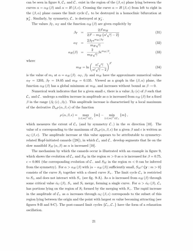
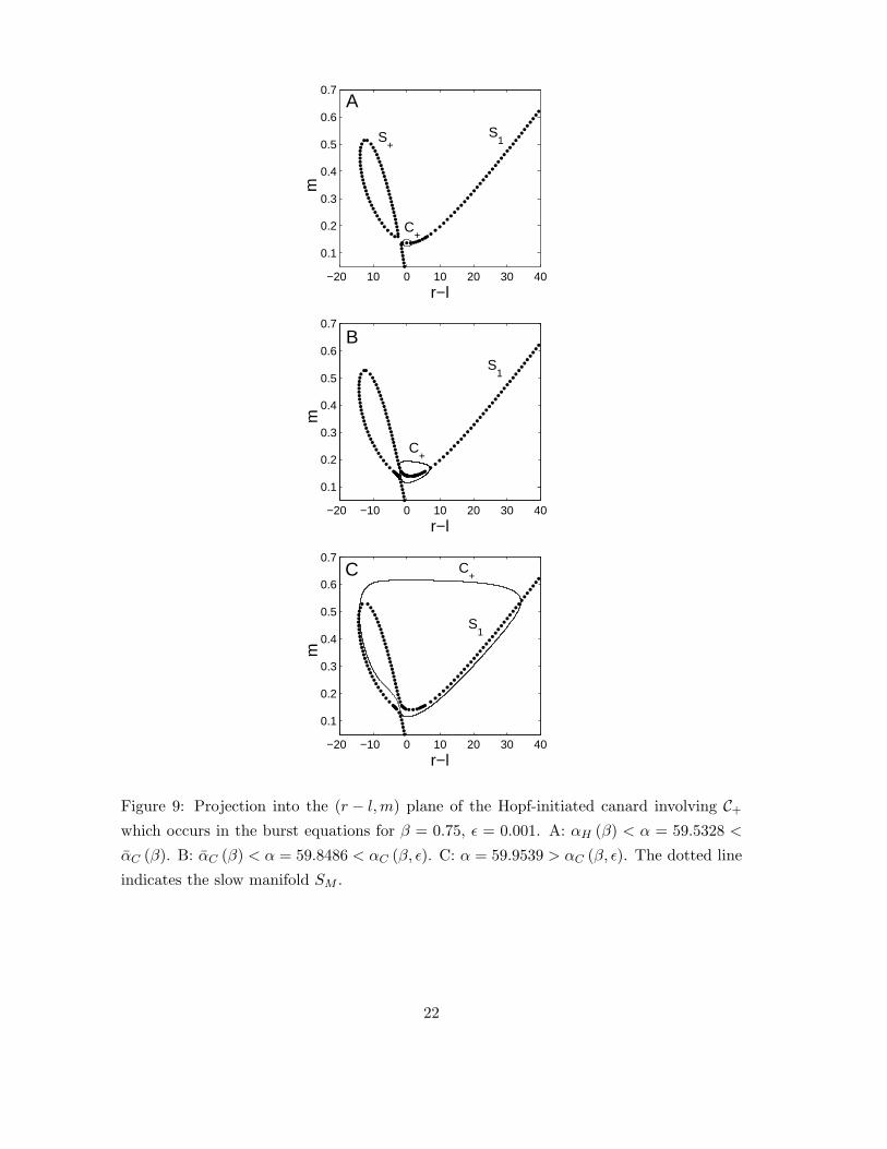
The mechanism by which the canards occur is illustrated with an example in figure 9,

which shows the evolution of C+ and SM in the region m > 0 as α is increased for β = 0.75,

ǫ = 0.001 (the corresponding evolution of C− and SM in the region m < 0 can be inferred

from the symmetry). For α > αH (β) with |α− αH (β)| sufficiently small, SM∩{y : m > 0}consists of the curve S1 together with a closed curve S+. The limit cycle C+ is restricted

to S1, and does not interact with S+ (see fig. 9-A). As α is increased from αH (β) through

some critical value αC (β), S+ and S1 merge, forming a single curve. For α > αC (β), C+

has portions lying on the region of S1 formed by the merging with S+. The rapid increase

in the amplitude of C+ as α increases through αC (β, ǫ) corresponds to the subset of this

region lying between the origin and the point with largest m value becoming attracting (see

figures 9-B and 9-C). The post-canard limit cycles {C+, C−} have the form of a relaxation

oscillation.

21

−20 10 0 10 20 30 40

0.1

0.2

0.3

0.4

0.5

0.6

0.7

r−lm

−20 −10 0 10 20 30 40

0.1

0.2

0.3

0.4

0.5

0.6

0.7

r−l

m

−20 −10 0 10 20 30 40

0.1

0.2

0.3

0.4

0.5

0.6

0.7

r−l

m

C+

C+

C+

A

B

C

S1 S

+

S1

S1

Figure 9: Projection into the (r − l,m) plane of the Hopf-initiated canard involving C+

which occurs in the burst equations for β = 0.75, ǫ = 0.001. A: αH (β) < α = 59.5328 <

αC (β). B: αC (β) < α = 59.8486 < αC (β, ǫ). C: α = 59.9539 > αC (β, ǫ). The dotted line

indicates the slow manifold SM .

22

6

α=αC

(β)

α=αH

(β)

α=Λ+β

α′

α=αC

(β,∈)

1.5

0

y1+, y

1−

C+, C

− (large−amplitude

relaxation oscillations)

0

C+, C

− (small−amplitude oscillations)

β

α

Figure 10: Bifurcations and attractors of the burst equations for 1.5 < β < 6, α < α′

and ǫ small. α = Λ+β is a line of supercritical nonsmooth pitchfork bifurcations at the

origin 0 = (0, 0, 0)T which creates the stable fixed points{

y+1 ,y

−1

}

. α = αH (β) is a line

of symmetry-related supercritical Hopf bifurcations at{

y+1 ,y

−1

}

which creates the stable

limit cycles {C+, C−}. α = αC (β, ǫ) is a line of symmetry-related Hopf-initiated canards

involving C+ and C−. α = αC (β) is the limiting curve of α = αC (β, ǫ) as ǫ → 0 (dotted

line).

Numerical computations indicate that the canard line α = αC (β, ǫ) and the line α =

αC (β) both intersect the Takens-Bogdanov point (βT , αT ). Moreover, as ǫ → 0, α =

αC (β, ǫ) converges to α = αC (β).

4.2.2 Bifurcations, attractors and simulated waveforms for 1.5 < β < 6, α < α′

Recall that the actual object of interest is the gaze time series {g (t) : t ≥ 0} of the full

model (1)-(6) for initial condition with v (0) = 0, n (0) = g (0) and m (0) = ∆g, as this

simulates a saccade of ∆g degrees from an initial gaze angle of g (0). In this section,

the various forms of g (t) that the model can produce will be discussed for the limited

parameter range 1.5 < β < 6, α < α′, for which biologically realistic time series were

previously found. Figure 10 is a plot of the burst system bifurcations and attractors for ǫ

small and (β, α) restricted to this region (compare with fig. 8). A range of the gaze time

series that can arise for parameters from this region is shown in figure 11. Each of these

will now be discussed in terms of the corresponding attractor, and the bifurcation giving

rise to the attractor.

23

0 0.1 0.2 0.30

2

4

6

8

10

12

14

0 0.1 0.2 0.30

2

4

6

8

10

12

14

0 0.1 0.2 0.30

0.1

0.2

0.3

0.4

0.5

0.6

0 1 2 3 40

0.1

0.2

0.3

0.4

0.5

0.6

0 0.2 0.4 0.6 0.8 1−12

−10

−8

−6

−4

−2

0

0 0.4 0.8 1.2 1.6−12

−10

−8

−6

−4

−2

0

0 0.2 0.4 0.6 0.8 1−20

−15

−10

−5

0

0 0.2 0.4 0.6 0.8 1−30

−20

−10

0

10

g(t)

t

A B

C D

E F

G H

Figure 11: Gaze time series {g (t) : t ≥ 0} generated by the full model (1)-(6) for initial

conditions with g (0) = v (0) = n (0) = 0 and m (0) = ∆g. A: α = 20, β = 3, ǫ = 0.001,

∆g = 10. Normometric saccade. B: α = 20, β = 3, ǫ = 0.015, ∆g = 10. Dynamic

overshoot. C: α = 206, β = 3, ǫ = 0.001, ∆g = 0.5. Hypometric saccade. D: α = 207.656,

β = 3, ǫ = 0.006, ∆g = 0.5. Small-amplitude nystagmus. E: α = 240, β = 3, ǫ = 0.004,

∆g = −10. Jerk CN. F: α = 240, β = 3, ǫ = 0.0048, ∆g = −10. Jerk with extended

foveation. G: α = 240, β = 3, ǫ = 0.006, ∆g = −10. Bidirectional jerk CN. H: α = 240,

β = 3, ǫ = 0.06, ∆g = −10. Pendular CN.

24

−200 −100 0 100 200 300 400 500−4

−2

0

2

4

6

8

10

12

r−lm

1

2

S1

Figure 12: Burst system trajectories corresponding to simulated normometric saccades.

Trajectory #1: α = 20, β = 3, ǫ = 0.001, ∆g = 10. Trajectory #2: α = 20, β = 3, ǫ =

0.015, ∆g = 10. The dotted line denotes the slow manifold SM . The stable manifold L0 is

orthogonal to this projection and passes through (0, 0). The gaze time series corresponding

to trajectories #1 and #2 are shown in figures 11-A and 11-B respectively.

Normometric saccades, hypometric saccades and dynamic overshoots: For α <

Λ+β with ǫ small, the origin 0 = (0, 0, 0)T is the unique attractor of the burst equations.

0 is a stable node of y = G (y) in this range, in the sense that it is a stable node of the

smooth systems y = G+(y) and y = G−(y) introduced in section 4.1.4. For α < Λ+β, SM

consists of the single curve S1. Since ǫ is small, y (t) contracts rapidly to S1 parallel to the

(r, l) plane, and then converges along S1 to the origin (see trajectory #1 of figure 12). The

corresponding motor error variable m (t) converges quickly to 0. Hence, as suggested by

approximation (16), the gaze time series has the form of a normometric (accurate) saccade

to g (0) + ∆g degrees which drifts back to zero like (g (0) + ∆g) e− t

TN . Figure 11-A shows

a simulated normometric saccade (cf. figure 1-A)

Increasing ǫ causes trajectories of y = G (y) to follow S1 less closely as they converge to

0. Indeed, for ǫ > 1

4(

Λ+−αβ

) , DG+ (0) has a pair of complex conjugate eigenvalues {µ, µ}

with Re {µ} < 0. Trajectories of the smooth systems y = G+(y) and y = G−(y) spiral

around the stable manifold L0 ={

(x, x, 0)T : x ∈ R

}

as they converge to the origin. Since

trajectories of the piecewise smooth system y = G (y) can be constructed by concatenating

sections of trajectories of y = G+(y) and y = G−(y), it follows that y (t) also spirals

around L0 as it converges to the origin (see trajectory #2 of figure 12). The motor error

m (t) converges to 0 by executing damped oscillations about 0. Thus, as suggested by

(16), the corresponding gaze time series g (t) has the form of a normometric saccade with

a post-saccadic damped oscillation about (g (0) + ∆g) e− t

TN , which resembles a dynamic

25

overshoot. A numerical example is shown in figure 11-B (cf. figure 1-B).

For Λ+β < α < αH (β) with ǫ small, the attractors are the symmetry-related pair of

fixed points{

y+1 ,y

−1

}

, which are stable nodes in this range. As trajectories cannot cross

the plane m = 0, y (t) → y+1 as t → ∞ if ∆g > 0 and y (t) → y−

1 as t → ∞ if ∆g < 0.

Thus, m (t) → sign(∆g)m1 as t→ ∞. If |∆g| is large compared to m1, g (t) has the form

of a normometric saccade, while if |∆g| is of the same order as m1, g (t) has the form of

a hypometric (under-shooting) saccade, as suggested again by approximation (16). Figure

11-C shows a simulated hypometric saccade.

Small-amplitude nystagmus and jerk CN: In the range α > αH (β) with ǫ small,

the attractors of the burst equations are the symmetry-related pair of stable limit cycles

{C+, C−}. Moreover, since trajectories cannot cross the plane m = 0, if ∆g > 0, y (t)

converges to C+, while if ∆g < 0, y (t) converges to C−. This situation was discussed in

section 3.3 where it was stated that if m (t) converges to a periodic function mS (t), then

g (t) converges to a periodic function gS (t) which is the result of applying a linear filter

to mS (t) (and consequently has the same period). Indeed, it was argued that if mS (t)

has no significant energy outside the angular frequency range (0.08, 55), then gS (t) ≈−mS (t− tg) + 〈mS (t)〉, where tg = 0.0115.

For αH (β) < α < αC (β, ǫ), C+ and C− are small-amplitude limit cycles. mS (t), and

hence gS (t), is therefore a small-amplitude periodic oscillation. The corresponding gaze

time series g (t) has the form of a normometric saccade with a post-saccadic small-amplitude

nystagmus. An example of such a waveform is shown in figure 11-D.

For α > αC (β, ǫ), C+ and C− are large-amplitude relaxation oscillations. Numerical

work suggests that for α > αC (β), the intersection of the slow manifold SM with the

plane m = m′ has greater extent in the positive r − l direction than in the negative r − l

direction, for m′ such that there is more than one point of intersection (cf. figures 9-B

and 9-C). Since m = − (r − l), this configuration of SM means that for α > αC (β, ǫ), the

contraction of C+ onto SM parallel to the (r, l) plane results in m changing rapidly from

small and positive to large and negative (cf. figure 9-C). (By symmetry, the contraction of

C− onto SM results in m changing rapidly from small and negative to large and positive).

Accordingly, mS (t) has the form of a slow drift away from m = 0 followed by a sudden

switch to a faster return towards m = 0 that resembles a jerk nystagmus. For ∆g > 0,

mS (t) resembles a left-beating jerk CN and for ∆g < 0, mS (t) resembles a right-beating

jerk CN. The approximation gS (t) ≈ −mS (t− tg) + 〈mS (t)〉 therefore implies that gS (t)

resembles a jerk nystagmus with a beat direction opposite to that of mS (t). For a given

∆g, the gaze time series g (t) has the form of a normometric saccade with a post-saccadic

oscillation which decays to a periodic jerk CN. The periodic oscillation is right-beating for

∆g > 0 and left-beating for ∆g < 0. Figure 11-E is an example of a simulated left-beating

jerk CN (cf. figure 1-C).

26

αC

(β) αC

(β) −

^

∈

αH

(β) αC

(β,∈′)

∈′

α

∈=∈C(α,β)

∈=∈G

(α,β)

α′

Figure 13: Schematic of the canard surface ǫ = ǫC (α, β) and the gluing-type bifurcation

surface ǫ = ǫG (α, β) in the (α, ǫ) plane for a fixed β with 1.5 < β < 6. The curve α = αC(β)

represents the projection onto the (β, α) plane of the intersection of ǫ = ǫC (α, β) with

ǫ = ǫG (α, β).

Jerk with extended foveation, bidirectional jerk and pendular CN: As ǫ is

increased in the range α > αC (β), the canards describe a surface ǫ = ǫC (α, β) in (α, β, ǫ)

space such that: i) the curve α = αC (β) is the intersection of ǫ = ǫC (α, β) with the

(β, α) plane, and ii) for a given value ǫ′ of ǫ, the curve α = αC (β, ǫ′) is the projection

onto the (β, α) plane of the intersection of ǫ = ǫC (α, β) with the plane ǫ = ǫ′. Numerical

work suggests that as ǫ is increased in (α, β, ǫ) space, the canard surface terminates by

intersecting a surface of gluing-type bifurcations, which will be written ǫ = ǫG (α, β). A

schematic of the curves ǫ = ǫC (α, β) and ǫ = ǫG (α, β) in the (α, ǫ) plane for a fixed β is

shown in figure 13 to aid their visualisation.

At ǫ = ǫG (α, β), C+ and C− merge, forming a single symmetry-invariant limit cycle

written as C. This bifurcation is qualitatively equivalent to a symmetric, smooth gluing

bifurcation of the saddlenode type ([26]), and is a result of C+ and C− undergoing simulta-

neous saddlenode homoclinic bifurcations at the origin in the smooth systems y = G+(y)

and y = G−(y) respectively. Figure 14 shows the gluing of the limit cycles as ǫ increases

through ǫ = ǫG (α, β) for α = 240 and β = 3.

Let α = αC (β) denote the curve corresponding to the projection onto the (β, α) plane

of the intersection of ǫ = ǫC (α, β) with ǫ = ǫG (α, β) (see figure 13). As ǫ is increased from

0 for α ∈ (αC (β) , αC (β)), the large-amplitude limit cycles C+ and C− undergo canards

becoming small-amplitude limit cycles. Increasing ǫ from 0 for α ∈ (αC (β) , α′) causes C+

and C− to undergo the gluing bifurcation. As ǫ→ ǫG (α, β)− in this range, the limit cycles

C+ and C− approach homoclinicity, resulting in mS (t) developing increasingly long periods

where it is approximately equal to 0. For ǫ < ǫG (α, β) with |ǫ− ǫG (α, β)| small, mS (t),

27

−400 −200 0 200 400−8

−6

−4

−2

0

2

4

6

8

r−lm

−400 −200 0 200 400−8

−6

−4

−2

0

2

4

6

8

r−l

m

−400 −200 0 200 400−8

−6

−4

−2

0

2

4

6

8

r−l

m

C+

C−

C

A

B

C

S1

S1

S1

Figure 14: Projection into the (r − l,m) plane of the nonsmooth gluing bifurcation which

occurs in the burst equations for α = 240, β = 3. A: ǫ = 0.0005. B. ǫ = ǫG (α, β) ≈0.00490167. C. ǫ = 0.008. The dotted lines denote the slow manifold SM .

28

and hence gS (t), resembles a jerk nystagmus with an extended foveation period. The gaze

time series g (t) has the form of a normometric saccade with a post-saccadic oscillation

which decays to a periodic jerk nystagmus with an extended foveation period. Figure 11-F

is an example of such a simulated waveform (cf. figure 1-D).

For ǫ > ǫG (α, β), provided that ǫ−ǫG (α, β) is not too large, C is a relaxation oscillation

with portions lying on SM (see figure 14-C). mS (t) is composed of slow drifts away from 0

followed by fast returns towards 0 in alternating directions, and resembles a bidirectional

jerk nystagmus. The approximation relating gS (t) and mS (t) implies that gS (t) also

resembles a bidirectional jerk nystagmus. g (t) has the form of a normometric saccade

which decays to a periodic bidirectional jerk oscillation, as can be seen in figure 11-G

(cf. figure 1-E). As ǫ → ǫG (α, β)+, C approaches homoclinicity, and gS (t) resembles a

bidirectional jerk nystagmus with an extended foveation period.

Increasing ǫ from ǫG (α, β) causes the limit cycle C to be successively less confined to

the slow manifold, and to lose the form of a relaxation oscillation. mS (t) loses its slow-

fast form, developing increasingly shorter foveation periods. For sufficiently large ǫ, mS (t)

is sinusoidal with no discernible foveation period, and resembles a pendular nystagmus

oscillation. gS (t) inherits this morphology, and g (t) has the form of a hypermetric (over-

shooting) saccade which decays to a periodic pendular nystagmus. Figure 11-H is an

example of a pendular nystagmus simulated by the model (cf. figure 1-F).

Other global bifurcations are observed numerically as ǫ is increased for (β, α) in the

range 1.5 < β < 6, α < αC (β), but these do not have any obvious biological interpretation.

In (α, β, ǫ) space, one of these bifurcation surfaces appears to intersect the canard surface

ǫ = ǫC (α, β) along the line where it intersects the surface of nonsmooth gluing bifurcations

ǫ = ǫG (α, β) [10].

The simulated eye movements generated in the parameter ranges discussed above are

summarised in figure 15. Numerical work indicates that αC (β) − αH (β) is a decreasing

function of β on (1.5, 6). Since mH < 1.5, αH (β) is increasing on (1.5, 6), from which it

follows thatαC (β) − αH (β)

αH (β)<αC (1.5) − αH (1.5)

αH (1.5)

in this range. Evaluating αH (1.5) and estimating αC (1.5) implies αC(1.5)−αH(1.5)αH(1.5) < 0.0055.

Hence, αC (β) ≈ αH (β) on (1.5, 6): the curves α = αH (β) and α = αC (β) lie very close

to each other in the (β, α) plane.

5 Implications of the model

5.1 CN may be caused by an abnormal saccadic braking signal

The current control systems view is that CN either results from an instability of the

oculomotor control subsystem responsible for gaze-holding, or an instability of the system

29

α (o

ff−re

spon

se m

agni

tude

)

6

α=αH

(β)

α=Λ+β

α′

α=αC

(β,∈)

1.5

[0]

[y1+, y

1−]

0

β (off−response range)

α=αC

(β) ^

Small ∈: normometric saccadeLarge ∈: dynamic overshoot

Small ∈: normometric saccade if |∆g|>>m1,

hypometric saccade if |∆g| is of the same order as m

1

Small−amplitude nystagmus [C+, C

−]

Jerk CN [C+, C

−]

∈<∈G

(α,β): jerk CN (extended foveation as ∈→∈G

(α,β)) [C+, C

−]

∈>∈G

(α,β): bilateral jerk (extended foveation as ∈→∈G

(α,β)) [C]

∈>>∈G

(α,β): pendular nystagmus [C]

Figure 15: Schematic plot showing the range of eye movements simulated by the saccadic

system model (1)-(6). The corresponding attractors of the burst equations (4)-(6) are

shown in square brackets. α = Λ+β is a line of nonsmooth pitchfork bifurcations at which

the origin 0 = (0, 0, 0)T goes unstable producing a pair of symmetry-related stable fixed

points{

y+1 ,y

−1

}

. α = αH (β) is a line of symmetry-related supercritical Hopf bifurcations

at which y+1 and y−

1 go unstable producing a pair of symmetry-related stable limit cycles

{C+, C−}. α = αC (β, ǫ) is a line of symmetry-related Hopf-initiated canards at which

C+ and C− undergo a sudden increase in amplitude, becoming relaxation oscillations.

α = αC (β) is the projection onto the (β, α) plane of the intersection of the canard surface

ǫ = ǫC (α, β) with the surface of nonsmooth gluing bifurcations ǫ = ǫG (α, β) (see figure 13).

As ǫ increases through ǫG (α, β) for α > αC (β), C+ and C− become homoclinic to the origin

and merge, producing a symmetry-invariant limit cycle C. α, β and ǫ represent respectively

the off-response magnitude, off-response range and response time of the saccadic burst

neurons.

30

responsible for tracking slowly moving targets (the smooth pursuit system) [33], [30], [21].

The saccadic system is invariably assumed to be functioning normally in the control models,

presumably as a consequence of the fact that CN subjects produce predominately accurate

saccades [45]. Possibly the most significant implication of the model is that it suggests

congenital nystagmus may in fact be a disorder of the saccadic system. Moreover, the

analysis implies that jerk CN is one of a range of disorders generated as the burst neuron

off-response magnitude α is increased (see figure 15).

Recalling that the off-response corresponds to a braking signal gives a physiological

interpretation of the modelled dysmetrias and oscillations. Hypometric saccades can be

attributed to a braking signal which has increased in strength to a level where it is causing

the eye to be brought to a halt before the target gaze angle is achieved. The oscillatory

disorders simulated by the model may be thought of as resulting from a braking signal of

sufficient strength to produce a significant movement of the eye in the opposite direction

to that of the saccade. This reverse motion in turn causes the onset of an oscillatory

instability through the mutual inhibition of the burst neurons.

The suggestion that CN is due to an abnormal braking signal is difficult to test since

it requires a normal braking signal/off-response to be accurately defined. Nonetheless, the

fact that a model of the fast eye movement system alone can generate both the slow and

fast phases of CN does indicate that the ability of CN subjects to generate normal saccades

is not sufficient basis to conclude that the instability must be a slow eye movement disorder.

5.2 The fast phases of CN may not be corrective

The model analysis implies that the slow-fast form of jerk and bidirectional jerk oscillations

may be a consequence of the geometry of an underlying slow manifold in the saccadic phase

space. This contrasts with the control models which assume that the fast phases of the

oscillations are corrective saccades that return the eye to the target following drift due to

a slow eye movement instability [33], [30], [21].

The alternative view proposed here is consistent with the finding that the peak velocities

of CN fast phases follows a saccadic main sequence distribution [9]. The segment of the

slow manifold along which trajectories that simulate normometric saccades contract to the

origin corresponds to the initial rapid movement of the eye towards the target gaze angle

(see trajectory #1 of figure 12). Consequently, the form of this segment determines the

relationship between the peak velocities and amplitudes of saccades that defines the main

sequence. As can be seen in figures 14-A and 14-C, the portions of the limit cycles C+,

C− and C which correspond to the fast phases of the corresponding simulated jerk and

bidirectional jerk oscillations all lie along this same segment: the fast phases therefore

follow the saccadic main sequence.

31

5.3 The most likely pathological oscillation is a jerk, bidirectional jerk

or pendular nystagmus

The analysis of the model implies that if the system is in the oscillatory regime α > αH (β),

the oscillation is likely to be a jerk, bidirectional jerk or pendular nystagmus. This follows

from the fact that αC (β) ≈ αH (β) on (1.5, 6), as discussed at the end of section 4.2.2.

Hence, as a result of the existence of the canard, only a small increase in the braking signal

strength α is required to push the system into the range α > αC (β) in which the possible

waveform types are those mentioned above. The intermediate small-amplitude oscillation

is unlikely to be observed (see figure 15).

This prediction is consistent with the findings of a recent major clinical eye movement

study [2]. Of the 161 CN subjects with a dominant waveform type used in the study,

all had oscillations with amplitude greater than 0.3 degrees: no subjects with sustained

small-amplitude oscillations were reported. Moreover, 73% of the subjects exhibited jerk,

bidirectional jerk, or pendular nystagmus oscillations, while 22% had oscillations which

were variations on these basic waveforms, such as pseudocycloid or pendular with foveating

saccades.

5.4 Dynamic overshoot is caused by reversals of the saccadic control

signal

It was argued in section 4.2.2 that increasing the burst neuron response time ǫ causes

burst system trajectories to follow the slow manifold SM less closely as they converge to

the origin. This results in oscillations of both the motor error signal m and the saccadic

control signal b = r − l as they converge to 0 (see figure 12). These oscillations are

converted by the muscle plant into a gaze signal g which oscillates about the desired gaze

angle g (0) + ∆g, and thus simulates a dynamic overshoot (see figure 11-B).

The ability of the model to generate dynamic overshoots in the range α < Λ+β is consis-

tent with the observation that normal subjects can exhibit dynamic overshoots in addition

to normometric saccades. Moreover, the suggestion that the overshoots are attributable to

oscillations of the saccadic control signal agrees with the predictions of a psychophysical

study of dynamic overshoots carried out by Bahill et al [12]. Bahill et al proposed that

the characterisation of the muscle plant as an overdamped harmonic oscillator implies that

the reversals in eye direction observed during dynamic overshoot are likely to be caused

by reversals of the saccadic control signal. Furthermore, they suggested that a possible

physiological cause of the reversals was post-inhibitory rebound firing of the burst neurons,

possibly accentuated by movements of the centre of rotation of the eye during saccades

[12].

The work presented here provides a simpler explanation for the reversals, namely the

spiralling of trajectories around the origin in the burst neuron firing rate versus motor

32

error phase plane, resulting from an increased burst neuron response time. The spiralling

of trajectories is independent of the inhibition between the right and left burst neurons,

and can be reproduced by a simplified model which does not incorporate mutual inhibition

terms in the equations for the burst neurons [7].

5.5 The evolution from jerk CN to bidirectional jerk CN is caused by a

gluing bifurcation

If ǫ is increased in the (β, α) range 1.5 < β < 6, α > αC (β), the model simulates the

transition from jerk nystagmus to bidirectional jerk and then pendular nystagmus observed

in some subjects as the initial gaze angle g (0) is varied, or their level of attention is reduced

[4], [5]. As ǫ corresponds to the speed at which the burst neurons respond to the motor

error signal m, an increase in ǫ might be interpreted as a decrease in the attention level

of the subject, and so the modelled waveform evolution is consistent with that observed

experimentally when the attention level is reduced. The evolution from jerk to bidirectional

jerk that is seen in some subjects as the gaze angle passes close to the neutral zone ([8])

cannot, however, be accounted for by the model in its current form, since g (0) is not a

parameter of the model. Additionally, the beat direction of the simulated jerk waveforms

is dependent on the required gaze displacement ∆g instead of g (0). These observations

suggest incorporating g (0) explicitly in the equations. The analysis of the basic model

presented here would provide the platform for a quantitative assessment of the effect of

such a modification.

Despite these limitations, the model does propose a specific underlying mechanism

for the jerk to bidirectional jerk transition, namely the merging of a pair of limit cycle

attractors in a gluing bifurcation. This is a novel explanation for the qualitative change

in the underlying neurobiological oscillator which could form the basis of a new technique

to control CN oscillations. A recent experimental study demonstrated that a transient

change from a unidirectional to a bidirectional jerk waveform could be induced in a CN

subject by forcing the target with a periodic waveform [19]. The waveform used in this

study was an unstable periodic orbit extracted from a previous recording of the subject’s

eye movements using the technique of So et al [38]. The gluing bifurcation mechanism

suggested here implies the possibility of establishing more sophisticated control over the

jerk waveform by using periodic forcing so as to bring the system close to homoclinicity.

Such a technique could have clinical applications, as the increased foveation times should

lead to the development of improved visual resolution.

Acknowledgements: The authors would like to thank Jerry Huke, Paul Glendinning and

Mark Muldoon for useful discussions. O. E. Akman was supported by a grant from the

Engineering and Physical Sciences Research Council.

33

References

[1] Abadi, R.V.: Mechanisms underlying nystagmus. J. R. Soc. Med. 95, 1–4 (2002)

[2] Abadi, R.V., Bjerre, A.: Motor and sensory characterisitics of infantile nystagmus.

Br. J. Ophthalmol. 86, 1152–1160 (2002)

[3] Abadi, R.V., Broomhead, D.S., Clement, R.A., Whittle, J.P., Worfolk, R.: Dynamical

systems analysis: A new method of analysing congenital nystagmus waveforms. Exp.

Brain Res. 117, 355–361 (1997)

[4] Abadi, R.V., Dickinson, C.M.: Waveform characteristics in congenital nystagmus.

Doc. Ophthalmol. 64, 153–167 (1986)

[5] Abadi, R.V., Dickinson, C.M., Pascal, E., Whittle, J., Worfolk, R.: Sensory and motor

aspects of congenital nystagmus. In: Schmid, R., Zambarbieri, D. (eds.) Oculomo-

tor Control and Cognitive Processes, pp. 249–262. Elsevier Science Publishers B. V.

(North-Holland) (1991)

[6] Abadi, R.V., Sandikcioglu, M.: Visual resolution in congenital pendular nystagmus.

Am. J. Optom. Phys. Opt. 52, 573–581 (1975)

[7] Abadi, R.V., Scallan, C.J., Clement, R.A.: The characteristics of dynamic overshoots

in square-wave-jerks and in congenital and manifest latent nystagmus. Vision Res.

40, 2813–2829 (2000)

[8] Abadi, R.V., Whittle, J.: The nature of head postures in congenital nystagmus. Arch.

Ophthalmol. 109, 216–220 (1991)

[9] Abadi, R.V., Worfolk, R.: Retinal slip velocities in congenital nystagmus. Vision Res.

29(2), 195–205 (1989)

[10] Akman, O.E.: Analysis of a nonlinear dynamics model of the saccadic system. Ph.D.

thesis, Department of Mathematics, University of Manchester Institute of Science and

Technology (2003)

[11] Arrowsmith, D.K., Place, C.M.: An Introduction to Dynamical Systems. CUP (1990)

[12] Bahill, A.T., Clark, M.R., Stark, L.: Dynamic overshoot in saccadic eye movements

is caused by neurological control signal reversals. Exp. Neurol. 38, 107–122 (1975)

[13] Bahill, A.T., Clark, M.R., Stark, L.: The main sequence, a tool for studying human

eye movements. Math. Biosci. 24, 191–204 (1975)

[14] Becker, W., Jurgens, R.: An analysis of the saccadic system by means of double step

stimuli. Vision Res. 19, 967–983 (1979)

34

[15] Becker, W., Klein, H.M.: Accuracy of saccadic eye movements and maintenance of

eccentric eye positions in the dark. Vision Res. 13, 1021–1034 (1973)

[16] Bedell, H.E., Loshin, D.S.: Interrelations between measures of visul acuity and param-

eters of eye movement in congenital nystagmus. Invest. Ophth. Vis. Sci. 32, 416–421

(1991)

[17] Boghen, D., Troost, B.T., Daroff, R.B., Dell’Osso, L.F., Birkett, J.E.: Velocity char-

acteristics of human saccades. Invest. Ophth. Vis. Sci. 13(8), 619–623 (1974)

[18] Broomhead, D.S., Clement, R.A., Muldoon, M.R., Whittle, J.P., Scallan, C., Abadi,

R.V.: Modelling of congenital nystagmus waveforms produced by saccadic system

abnormalities. Biol. Cybern. 82, 391–399 (2000)

[19] Clement, R.A., Abadi, R.V., Broomhead, D.S., Whittle, J.P.: Periodic forcing of

congenital nystagmus. In: Boccaletti, S., Gluckman, B.J., Kurths, J., Pecora, L.M.,

Spano M.L. (eds.) Experimental Chaos (Proceedings of the 6th Experimental Chaos

Conference, Potsdam, Germany, 2001). AIP (2002)

[20] Clement, R.A., Whittle, J.P., Muldoon, M.R., Abadi, R.V., Broomhead, D.S., Akman,

O.: Characterisation of congenital nystagmus waveforms in terms of periodic orbits.

Vision Res. 42, 2123–2130 (2002)

[21] Dell’Osso, L.F.: Nystagmus basics: Normal models that simulate dysfunction. In:

Hung, G.K., Ciuffreda, K.J. (eds.) Models of the Visual System, pp. 711–739. Kluwer

Academic (2002)

[22] Dell’Osso, L.F., Daroff, M.D.: Congenital nystagmus waveforms and foveation strat-

egy. Doc. Ophthalmol. 39, 155–182 (1975)

[23] Ditchburn, R.W.: Eye Movements and Visual Perception. Clarendon Press, Oxford

(1973)

[24] Enderle, J.D.: Neural control of saccades. In: Hyona, J., Munoz, D.P., Heide, W.,

Radach, R. (eds.) The Brain’s Eye: Neurobiological and Clinical Aspects of Oculomo-

tor Research, vol. 140, pp. 21–49. Elsevier, Amsterdam (2002)

[25] Gancarz, G., Grossberg, G.: A neural model of the saccade generator in the reticular

formation. Neural Networks 11, 1159–1174 (1998)

[26] Glendinning, P.: Global bifurcations in flows. In: Bedford, T., Swift, J. (eds.) New

Directions in Dynamical Systems, pp. 120–149. CUP (1988)

[27] Golubitsky, M.: Singularities and Groups in Bifurcation Theory. Springer Verlag

(1985)

35

[28] Guckenheimer, J., Hoffman, K., Weckesser, W.: Numerical computation of canards.

Int. J. Bifurcat. Chaos 10(12), 2669–2687 (2000)

[29] Guckenheimer, J., Holmes, P.: Nonlinear Oscillations, Dynamical Systems and Bifur-

cations of Vector Fields. Springer Verlag (1983)

[30] Harris, C.M.: Problems in modelling congenital nystagmus: Towards a new model. In:

Findlay, J.M., Walker, R., Kentridge, R.W. (eds.) Eye Movement Research: Mecha-

nisms, Processes and Applications, pp. 239–253. Elsevier, Amsterdam (1995)

[31] Hirsch, M.W., Smale, S.: Differential Equations, Dynamical Systems and Linear Al-

gebra. Academic Press (1974)

[32] Kreyszig, E.: Advanced Engineering Mathematics, 7th edn. John Wiley (1993)

[33] Optican, L.M., Zee, D.S.: A hypothetical explanation of congenital nystagmus. Biol.

Cybern. 50, 119–134 (1984)

[34] Robinson, D.A.: The mechanics of human saccadic eye movements. J. Physiol. 174,

245–264 (1964)

[35] Robinson, D.A.: Models of the saccadic eye movement control system. Kybernetik

14, 71–83 (1973)

[36] Scudder, C.A.: A new local feedback model of the saccadic burst generator. J. Neu-

rophysiol. 59, 1455–1475 (1988)

[37] Shelhamer, M.: On the correlation dimension of optokinetic nystagmus eye move-

ments: Computational parameters, filtering, nonstationarity and surrogate data. Biol.

Cybern. 76, 237–250 (1997)

[38] So, P., Ott, E., Sauer, T., Gluckman, B.J., Grebogi, C., Schiff, S.: Extracting unstable

periodic orbits from chaotic time series data. Phys. Rev. E 55, 5398–5417 (1997)

[39] Sparks, D.L.: The brainstem control of saccadic eye movements. Nature Rev. Neurosci.

3, 952–964 (2002)

[40] Stark, J.: Invariant graphs for forced systems. Physica D 109, 163–179 (1997)

[41] Tusa, R.J., Zee, D.S., Hain, T.C., Simonsz, H.J.: Voluntary control of congenital

nystagmus. Clin. Vision Sci. 7, 195–210 (1992)

[42] Van Gisbergen, J.A.M., Robinson, D.A., Gielen, S.: A quantitative analysis of gen-

eration of saccadic eye movements by burst neurons. J. Neurophysiol. 45, 417–442

(1981)

36

[43] Westheimer, G.: Mechanism of saccadic eye movements. Arch. Ophthalmol. 52, 710–

724 (1954)

[44] Westheimer, G., McKee, S.P.: Visual acuity in the presence of retinal image motion.

J. Opt. Soc. Am. 65, 847–850 (1975)

[45] Worfolk, R., Abadi, R.V.: Quick phase programming and saccadic re-orientation in

congenital nystagmus. Vision Res. 31(10), 1819–1830 (1991)

[46] Zeeman, E.C.: Differential equations for the heartbeat and nerve impulse. In:

Waddington, C.H. (ed.) Towards a Theoretical Biology, pp. 8–67. University Press,

Edinburgh (1972)

37