This article was downloaded by: [129.130.252.222]On: 19 July 2014, At: 09:17Publisher: RoutledgeInforma Ltd Registered in England and Wales Registered Number: 1072954 Registered office: Mortimer House,37-41 Mortimer Street, London W1T 3JH, UK

Applied Financial EconomicsPublication details, including instructions for authors and subscription information:http://www.tandfonline.com/loi/rafe20

Extreme returns and the contagion effect between theforeign exchange and the stock market: evidence fromCyprusStelios D. Bekiros a & Dimitris A. Georgoutsos aa Department of Accounting and Finance , Athens University of Economics and Business , 76Patission Str., 104 34 Athens, GreecePublished online: 26 Nov 2007.

To cite this article: Stelios D. Bekiros & Dimitris A. Georgoutsos (2008) Extreme returns and the contagion effect betweenthe foreign exchange and the stock market: evidence from Cyprus, Applied Financial Economics, 18:3, 239-254, DOI:10.1080/09603100601018823

To link to this article: http://dx.doi.org/10.1080/09603100601018823

PLEASE SCROLL DOWN FOR ARTICLE

Taylor & Francis makes every effort to ensure the accuracy of all the information (the “Content”) containedin the publications on our platform. However, Taylor & Francis, our agents, and our licensors make norepresentations or warranties whatsoever as to the accuracy, completeness, or suitability for any purpose of theContent. Any opinions and views expressed in this publication are the opinions and views of the authors, andare not the views of or endorsed by Taylor & Francis. The accuracy of the Content should not be relied upon andshould be independently verified with primary sources of information. Taylor and Francis shall not be liable forany losses, actions, claims, proceedings, demands, costs, expenses, damages, and other liabilities whatsoeveror howsoever caused arising directly or indirectly in connection with, in relation to or arising out of the use ofthe Content.

This article may be used for research, teaching, and private study purposes. Any substantial or systematicreproduction, redistribution, reselling, loan, sub-licensing, systematic supply, or distribution in anyform to anyone is expressly forbidden. Terms & Conditions of access and use can be found at http://www.tandfonline.com/page/terms-and-conditions

Applied Financial Economics, 2008, 18, 239–254

Extreme returns and the contagion

effect between the foreign

exchange and the stock market:

evidence from Cyprus

Stelios D. Bekiros* and Dimitris A. Georgoutsos

Department of Accounting and Finance, Athens University of Economics and

Business, 76 Patission Str., 104 34 Athens, Greece

In this article we apply the Extreme Value Theory (EVT) in order to

estimate the Value-at-Risk (VaR) and the correlation of extreme returns

for two inherently unstable markets; the foreign exchange and the stock

market. We also derive the corresponding VaR estimates from more

‘traditional’ methods of estimation on daily returns of the US dollar/

Cyprus pound exchange rate and the Cyprus stock exchange general index.

The main conclusion we reach is that the more heavy-tailed distributed a

series is the more accurate the loss predictions are from the application of

the EVT. We also show that the conditional correlation index of the

extreme returns of those two markets remained almost constant through-

out the backtesting period that was characterized by ‘bear’ market

conditions.

I. Introduction

Over the last 15 years we have witnessed a massive

inflow of portfolio capital in emerging equity markets

as the result of their liberalization. It is being reported

that the average annual net private capital flow to

developing countries over the period 1983 to 1988

was $15.1 billion, whereas during the period 1989 to

1995 the figure surged to $107.6 billion. As a result of

that, the market capitalization as a proportion to

GDP rose at an unprecedented rate to over 70% in

some countries (Singh and Weisse, 1998). Among the

forces that drove advanced country flows to devel-

oping markets one could identify the lower growth

prospects in developed country stock markets, the

desire of institutional investors to diversify their

portfolios as well as the ability of foreign investors to

move funds in and out of emerging stock markets

following their external liberalization. At the same

time developing country corporations resorted to

stock market finance because the relative cost of

equity capital fell as a result of the large share price

rises during the course of 1990s’ and the large

increase of real interest rates in the aftermath of

financial deregulation.Notwithstanding those positive developments,

many empirical studies have confirmed much greater

share price volatility in emerging markets than in

more mature ones. This can be attributed to many

reasons ranging from the fact that firms in emerging

markets have not established market reputations to

the speculative nature of the portfolio capital inflows

(Tirole, 1991). The first factor explains why the share

pricing process is ‘noisy’ and the fact that only

a limited number of shares, which however account

for a considerable part of total market capitalization,

*Corresponding author. E-mail: bekiros@aueb.gr

Applied Financial Economics ISSN 0960–3107 print/ISSN 1466–4305 online � 2008 Taylor & Francis 239http://www.tandf.co.uk/journalsDOI: 10.1080/09603100601018823

Dow

nloa

ded

by [

] at

09:

17 1

9 Ju

ly 2

014

are actively traded. The second factor has beendocumented in many empirical studies that point tothe fact that the surge of capital towards manyemerging markets was not based on an improvementof their ‘fundamentals’. This investment strategy hasbeen rationalized from the imitative and bandwagonbehaviour of investors who endeavour to conform tothe actions of the ‘average’. This kind of behaviourhowever leads to sudden reversals of the decisionson which the capital inflows were based initially andit makes the emerging markets especially proneto internal and external shocks. Furthermore, itgenerates negative interactions between theforeign exchange and equity markets with adverserepercussions to crucial macroeconomic variables(Krugman, 1995).

The connection between the foreign exchange andthe equity market has been theoretically investigatedin the literature concerning the determinants ofexpected international asset returns. In the interna-tional version of the capital asset pricing model,developed by Solnik (1983) and Adler and Dumas(1983), the expected returns depend on a commonrisk factor which is the return on a value-weightedworld equity market portfolio, hedged againstcurrency risk. Unfortunately, the amount of currencyhedging that enters in this common factor depends onthe individuals’ utility function and relative wealth.Given the absence of information concerning thoselast issues, the model is empirically equivalent to amulti-risk factor model with a world equity marketportfolio factor and currency risk factors. Under veryrestrictive assumptions, e.g. that the purchasingpower parity holds exactly at every instant, it hasbeen shown by Grauer et al. (1976) that the worldequity market portfolio would be the sole interna-tional risk factor. The significance of the exchangerate risk as a possible determinant of asset returns hasbeen identified in a number of studies coveringvarious countries, sectors of the economy andperiods. Using cointegration analysis and errorcorrection models, Ajayi and Mougoue (1996)found evidence in favour of dynamic linkagesbetween stock prices and exchange rates for eightindustrialized countries over the period 1985 to 1991.Recently, Harvey et al. (2002) used a latent factortechnique and showed that two factors, which arerelated to the expected return on the world marketportfolio and to the foreign exchange risk, aresufficient to explain the conditional variation in theequity indices returns for 16 Organization forEconomic Coopertation and Development (OECD)countries.

The earlier discussion has highlighted the signifi-cant volatility of equity returns in emerging capital

markets, the interconnection between the equities andforeign exchange markets, especially in crises periods,and the presence of the foreign exchange risk inpricing the equities in emerging capital markets. Inthis study we attempt first, to measure the risk ofthose two markets by applying the Value-at-Risk(VaR) methodology. By definition, VaR is anestimate of the maximum expected loss on aninvestment, over a given time period, at a givenconfidence level. It turns out that VaR summarizes ina single number the downside risk of the portfolioand this explains its widespread popularity amongpractitioners and academics alike. However, VaR isnot a coherent risk measure since it does not alwayssatisfies the axiom of subadditivity according towhich diversification is beneficial to risk minimiza-tion (Artzner et al., 1999). We provide an extensivelist of VaR estimates that are based on variousmethodologies for the estimation of the SD ofreturns. Those ‘traditional’ techniques have beenextended to incorporate the Extreme Value Theory(EVT) which provides the necessary asymptotictheorems for modelling explicitly the tails of thedistribution of returns. The out-of-sample predictiveability of the various techniques has been evaluatedby means of the criterion on coverage probabilitydeveloped by Christoffersen (1998).

The issue of the contagion between the foreignexchange and the equities markets is a more delicateone since the correlation of the returns of those twomarkets might not be the appropriate measure ofdependence. It is well established now that calculatingthe correlation index on different sub-periods in orderto establish a possible breakdown between twomarkets is the wrong procedure. The reason is thatfrom a completely statistical perspective one wouldexpect higher correlations during periods of highvolatility. Boyer et al. (1999) demonstrate thatsplitting a sample of data into high and low volatilitysub-samples can yield misleading results, because sucha procedure introduces a selection bias problem whichmight suggest a correlation breakdown regardless ofwhether the coefficient has changed. Moreover, thefocus on correlation and hence on linear dependence isentirely appropriate when the joint distribution of thedata is multivariate normal or, more generally,multivariate elliptic. This of course is not the casewhen we measure the dependence at crises periods.

The structure of this article is as follows. In thenext section, we present analytically the estimationprocess of the VaR when the EVT is applied. Twoalternative techniques are applied; the POT and theBlocks Minima. The first one identifies as extremeobservations all those that exceed a pre-chosenthreshold while the second one splits the sample in

240 S. D. Bekiros and D. A. Georgoutsos

Dow

nloa

ded

by [

] at

09:

17 1

9 Ju

ly 2

014

nonoverlapping blocks and chooses the lowest returnin each one. We then proceed with the derivation ofmeasures of dependence when returns are not multi-variate normally distributed. In Section III we presentthe estimation results that have been derived fromdaily returns of the Cyprus General Index and the USdollar/Cyprus pound exchange rate. We concludeafterwards.

II. Value-at-Risk Models and ExtremalDependence: the Extreme ValueTheory Approach

Computing value-at-risk for a single position

The most critical issue in risk management is theestimation of accurate risk measures that relate to theprobabilities of having a large negative realization ofa random variable. One way to approach this issue isto employ one of the distributions that have beenadvanced in the literature for modelling high fre-quency financial returns exhibiting excess kurtosis(e.g. stable distributions, the Student-t or the ARCHprocess). One problem with this approach is that thefitted distribution might be heavily affected by thevast majority of the observations that lie in the centreof the density, whereas interest is really focused uponthe tails. One further problem is that the comparisonbetween the competing models is hampered by thefact that those models are not nested. Consequently,research has been directed into modelling the ‘tails’ ofthe distribution separately and the interest here lies inthe estimation of the so-called tail index which is agood indicator for the shape of the distribution ofextreme returns. Empirical articles by, inter alia,Blattberg and Gonedes (1974); Akgiray and Booth,(1988); Jansen and deVries (1991), attempted toanswer whether the financial series are consistentwith stable laws or equivalently whether or not thesecond moment is finite.1

In this article, we follow the second approachunder which the various methodologies by whichextreme values may be statistically modelled separateinto two forms: methods for maxima (or minima)over fixed intervals and methods for exceedances overhigh (low) thresholds. The first one is often referred

to as the Block Maxima (Minima) (BM) method and

the second one as the POT method.Under the BM method the data are divided into m

blocks with n observations in each block correspond-

ing to n trading intervals. Extremes are then defined

as the maximum (or minimum) of the n random

variables Y1,Y2, . . . ,Yn and let Zn¼

max(Y1,Y2 , . . . ,Yn) denote this maximum.2 Fisher

and Tippett (1928) have shown that for returns Yt

that are independent and drawn from the same

distribution F, if there exist normalizing constants wn

and qn such that

limn!1

PZn � wn

qn � y

� �¼ lim

n!1Fnðqnyþ wnÞ ¼ HðyÞ ð1Þ

for some nondegenerate limit distribution H, then H

belongs to three families of distributions which

according to Jenkinson (1955) can be represented

by the Generalized Extreme Value distribution

(GEV), i.e.

HðyÞ ¼expð�ð1þ �yÞ�1=�

Þ if � 6¼ 0

expð�e�yÞ if � ¼ 0

( ),

ðy, �Þ 2 R, ð1þ �yÞ � 0 ð2Þ

According to the tail index value, �, three types of

extreme value distributions are distinguished: the

Frechet distribution (�>0), the Weibull distribution

(�<0) and the Gumbel distribution (�¼ 0). It follows

therefore that, whatever the distribution of the

original random variables the limiting distribution

of the maximum has a small set of possible

distributions. If (1) holds, we shall say that F belongs

to the maximum domain of attraction of H and write

F2MDA(H�). Essentially all the common, contin-

uous distributions of statistics are in MDA(H�) for

some value of �. Thus the normal, lognormal,

exponential and gamma distributions correspond to

the Gumbel case. The heavy tailed distributions

typically encountered in finance are in the Frechet

domain of attraction.3 This class includes the Pareto,

Cauchy Student-t and mixture distributions.We do not know the underlying distribution of

financial returns but since there is a growing

consensus that they have heavy tails the Frechet

limit will be the relevant case. In accordance to the

theorem presented above we fit the GEV distribution

1The tail probabilities of stable distributions approximate those of the Pareto distribution. Therefore, the tail index of thePareto distribution that is fitted on the extremes conveys information on the shape of the entire density function, (Campbellet al., 1997).2 In the text we present the theoretical results for the maximum only. However, the results for the mimimum are identicalsince: max(Y1,Y2, . . . ,Yn)¼�min(�Y1,�Y2 , . . . ,Yn), (Longin, 2000).3De Haan (1976) has derived the necessary conditions for the moments to exist when the underlying distributionF2MDA(H�). For a heavy tailed distribution �>0 the kth moment does not exist if k� (1/�).

Extreme returns and the contagion effect between the FE and the stock market 241

Dow

nloa

ded

by [

] at

09:

17 1

9 Ju

ly 2

014

H�,�,�¼H[(Zn��)/�)] on the standardized data ofblock minima, (Zn��)/�. The location parameter �and the positive scale parameter � take care of theunknown sequences of normalizing constants wn andqn. Let us now define with Rn,k a level that we expectto be exceeded, on average, in one n-block for every kn-blocks. If we believe that maxima in blocks oflength n follow the generalized extreme valuedistribution, the Rn,k is a quantile of this distribution,that is a VaR estimate, and from (2) we can derive

Rn,k ¼H�1�,�,�

1�1

k

� �¼�

_��_

�_

1� � log1�1

k

� �� ���_

0@

1A

ð3Þ

where �, � and � have been substituted for theirmaximum likelihood estimates. If returns Yi areindependent then the following holds:

1� 1

k

� �¼ PðY1 � Rn, k, . . . ,Yn � Rn, kÞ ¼ FnðRn, kÞ

ð4Þ

so the (1� 1/k) quantile, Rn,k, for the distribution ofZn corresponds to the (1� 1/k)1/n quantile of themarginal distribution of Yi (Longin, 2000). Supposefor example that we consider our model for annual(261 days) maxima. Then, the return that we expect tobe exceeded once every 20 years, the 20-year returnlevel, corresponds to the (0.95)(1/261)¼ 0.9998 quantile.

The results we presented above have been derivedfor the case of stationary, identically and indepen-dently (i.i.d.) distributed random variables. InLeadbetter et al. (1983) we find two technicalconditions under which the extreme value theoremsextend to conditional processes. The first conditionrequires that the extremes of a process are weaklydependent only in the long run (Longin (2000) for acondition of the degree of dependence that must besatisfied). Considering that the dependence in returnsstems from different volatility regimes that changewith time, it is not unreasonable to assume that in thelong run extreme returns are effectively independent.The second condition requires that no clusters ofextreme values appear. However, since the financialtime series show clusters of volatility that lead toclusters of large values the second condition isunrealistic and we must look more carefully into theissue of de-clustering the extreme values so that theyappear as approximately independent (McNeil,1998). Let (Yn) be a stationary variable with marginaldistribution F, where Zn¼max(Y1 , . . .,Yn) and ð ~YnÞ

an associated independent process with the same

marginal distribution F where ~Zn ¼ maxð ~Y1, . . . , ~YnÞ.

The extremal index, for large n, is defined as a real

number 0� �� 1 such that:

PfZn � Rn, kg � P�f ~Zn � Rn, kg ¼ Fn�ðRn, kÞ ð5Þ

Under this definition the maximum of n observations

from the noni.i.d. series behaves like the maximum of

n� observations from the associated i.i.d. variable.

It can be also shown that the maxima Zn of a noni.i.d.

series converge in probability to H�(Y) and from

Equation 3 that the VAR estimate is given by

Rn, k ¼ Y1=n�ð1�1=kÞ (McNeil, 1998; Longin, 2000).

A natural asymptotic estimator of � is:

� ¼ n�1 �ln 1� Ku=mð Þ

ln 1�Nu=ðm � nÞð Þð6Þ

where Nu is the number of exceedances of the

threshold u, Ku is the number of blocks the threshold

is exceeded and m, n, stand for the number of blocks

and days in each block respectively, (Smith and

Weissman, 1994). The asymptotic derivation of the

previous equation suggests that we should attempt to

keep both m and n large (McNeil, 1998).Under the Peaks over Threshold, POT, method we

fix a high threshold u and look at all exceedances y

over u. If F(Y) represents the distribution function of

returns Y, then the cumulative distribution of the

u-xceedances, denoted by Fu(y), is defined by:

FuðyÞ ¼ P Y � yþ u Y> uj½ � ¼Fðyþ uÞ �FðuÞ

1�FðuÞ, x> 0

ð7Þ

where 0� y< x0� u and x0�1 is the (finite or

infinite) right endpoint of F. Balkema–de Haan

(1974) and Pickands (1975), studied the asymptotic

behaviour of threshold exceedances and proved for a

large class of the underlying distribution Fu(y) that its

limiting distribution, as the threshold is raised, is the

Generalized Pareto Distribution (GPD) which is

given by:

GðyÞ ¼ 1�1þ �y

�

� ��1=�

, � 6¼ 0

GðyÞ ¼ 1� expð�yÞ, � ¼ 0

ð8Þ

where � is the tail index, �>0 the scale parameter

and the support is y� 0 when �>0 and 0< y<

�(�/�) when �<0.4 Essentially all the common

continuous distributions of statistics belong in this

class of distributions. For example the case �>0

4An extremal index, which measures the degree of clustering of extremes above the threshold, can be obtained in this methodas well by using the runs estimator (Smith and Weissman, 1994).

242 S. D. Bekiros and D. A. Georgoutsos

Dow

nloa

ded

by [

] at

09:

17 1

9 Ju

ly 2

014

corresponds to heavy tailed distributions such as thePareto and Student-t. The case �¼ 0 corresponds todistributions like the normal or the lognormal whosetails decay exponentially. The short-tailed distribu-tions with a finite endpoint such as the uniform orbeta correspond to the case �<0.

We now discuss how the results of the last sectioncan be used to estimate VaRs. Let yi

� �Nu

i¼1be the

sample of exceedances of a high threshold, u, with itssize being Nu. If we assume that those Nu excessesare i.i.d. with an exact GPD distribution then themaximum likelihood estimates of the GPD param-eters � and � are consistent and asymptoticallynormal as Nu!1 provided that �>�1/2 (Smith,1987). We define �FuðyÞ ¼ 1� FuðyÞ and then byemploying the identity shown in (7) we have:

�Fðuþ yÞ ¼ �FðuÞ �FuðyÞ ð9Þ

In (7) we substitute �Fðuþ yÞ ¼ 1� p, the confidencelevel, �FðuÞ ¼ Nu=n, the proportion of the data in thetail and FuðVaRð1� pÞ � uÞ ¼ GðVaRð1� pÞ � uÞwhere G represents the GPD with the parameters �and � substituted for the maximumlikelihood estimates. From (9) then we can estimatep-quantiles as:

VaRð1� pÞ ¼ uþ�

�

nð1� pÞ

Nu

� ���

�1

( )ð10Þ

Measuring extreme value dependence

Estimating dependence between risky asset returnsis of paramount importance in risk management.Unfortunately, the conventional measure of depen-dence, the correlation index, is appropriate only whenthe assumption of multivariate normally distributedreturns is tenable. Correlation is a measure of thelinear association between two variables since byconstruction it assigns the same weights on alldeviations from the mean. There are cases howeverwhere the extreme realizations have a dependencestructure that is different from the rest of the sample.More formally, it has been shown that a class ofmultivariate distributions where the standard correla-tion approach to dependence is natural and unprob-lematic is the elliptical distributions. The ellipticaldistributions, of which the multivariate normal is aspecial case, are distributions whose density isconstant on ellipsoids. In two dimensions, thecontour lines of the density surface are ellipses.Interestingly, a multivariate distribution with uncor-related components is not a distribution with

independent components. It provides an example

where zero correlation of risks does not imply

independence of risks. Only in the case of the

multivariate normal can the lack of correlation be

interpreted as independence.Copulas, or dependence functions, represent a way

of trying to extract the dependence structure from the

joint distribution. This is being accomplished by

separating the joint distribution into a part that

describes the dependence structure and a part that

describes the marginal behaviour only. Let us

consider a q-dimensional vector of random returns

denoted by Y0 ¼ (Y1,Y2, . . . ,Yq)0 with marginal dis-

tributions F1, . . . ,Fq. The joint distribution function

C of (F1(Y1), . . . ,Fq(Yq))0 is then called the copula of

the random vector Y0 ¼ (Y1,Y2, . . . ,Yq)0. It follows

then that:

Fðy�1, . . . , y�qÞ ¼ Prob½Y1 � y�1, . . . ,Yq � y�q�

¼ CðF1ðy�1Þ, . . . ,Fqðy

�qÞÞ ð11Þ

where y�i ¼ ui þ yi and yi refers to the exceedance of

Yi over the threshold ui. Moreover, Sklar (1959)

proved that F has a unique copula if the marginal

distributions are continuous. However, if there are

discontinuities in one or more marginals then there is

more than one copula representation for F. In either

case, it makes sense to interpret C as the dependence

structure of F. As with rank correlation, the copula

remains invariant under (strictly) increasing transfor-

mations of the risks; the marginal distributions

clearly change but the copula remains the same.Once the problem is to study the dependence

structure of extreme returns, the multivariate return

exceedances distribution must be defined. As with the

univariate case the exact distribution is not exactly

known and therefore we have to consider asymptotic

results. The possible limit nondegenerate distribution

however must satisfy two properties; first, that the

marginal distributions are generalized Pareto distri-

butions and second that the correlation increases at

high confidence intervals. The two properties take

care of the fat-tails feature of univariate returns and

of the empirical regularity of correlations increases at

crisis periods. The second property is satisfied by the

logistic model in the bivariate extreme value family

that is given by:

Cðs, tÞ ¼ PrðS � s, T � tÞ

¼ exp � s�ð1=aÞ þ t�ð1=aÞ� �ah i

, 0 < a � 1

ð12Þ

(Tawn, 1988; Longin and Solnik, 2001). In order to

dissociate the correlation structure from the marginal

Extreme returns and the contagion effect between the FE and the stock market 243

Dow

nloa

ded

by [

] at

09:

17 1

9 Ju

ly 2

014

distributions the bivariate return exceedances havebeen transformed to unit Frechet margins,S ¼ �1= logFu1 ðy1Þ, T ¼ �1= logFuu ðy2Þ, whereFui ðyiÞ is the GPD of exceedance yi. The asymptoticdependence of (S,T) is defined by:

� ¼ lims!1

PrT � s

S � s

� �ð13Þ

where 0��� 1, and the two variables are termedasymptotically dependent if �� 0 and asymptoticallyindependent if �¼ 0. The relationship between thecoefficient �, of Equation 12 and � is given by�¼ 2� 2� so when the variables are exactly indepen-dent �¼ 1 and �¼ 1 while when � 1 the variables areasymptotically dependent to a degree depending on �.

Since we have chosen the two thresholds, thebivariate distribution of return exceedances is thendescribed by seven parameters: the two tail probabil-ities, the dispersion parameters and the tail indexes ofeach variable, and the dependence parameter of thelogistic function. The parameters of the model areestimated by the maximum likelihood method. In thebivariate case, the correlation coefficient of extremesis related to the coefficient of dependence by�¼ 1� �2 (Tiago de Oliveira, 1973).

III. Empirical Evidence

We implement the various VaR estimation techniqueson daily returns of the US dollar/Cyprus poundexchange rate and the Cyprus Stock Exchangegeneral index (CGI). The series cover the period 1April 1996 to 27 April 2001.5 Both series have beentested for the null hypothesis of being normal and thishas been rejected under both the Kolmogorov–Smirnov test statistic and the �2 test for normality.The period 30 April 2001 to 19 April 2002 has beenreserved for backtesting the predictive performanceof the alternative models. Our first goal is to validatethe adequacy of competing VaR methodologiesthrough the backtesting exercise. On the one handwe examine ‘conventional’ models that encompassboth parametric and simulating techniques and onthe other hand the two approaches offered by the

Extreme Value Theory. The parametric models havebeen estimated under various specifications of theconditional distribution of the error generatingprocess that is the Gaussian (N), the student (t) andthe Generalized Error Distribution (GED).Moreover, each one of those models has beenestimated under various specifications for the condi-tional variance process which is alternatively approxi-mated by a Moving Average process, theExponentially Weighted Moving Average (EWMA)specification and the GARCH(1,1) model. The samethree specifications of the conditional variance areemployed with the Monte Carlo simulation method.A more detailed presentation of these techniques isgiven in appendix A.

For the Blocks method we analysed monthly andquarterly minima and the fit of the Frechet distribu-tion on both sets of sample minima was found to beadequate. For each block maximum (minimum) thecorresponding crude residual is defined to be:

Wi ¼ 1þ�

�

� �ðZi � �Þ

� ��ð1=�Þ

ð14Þ

According to Cox and Snell (1968) these should bei.i.d. unit exponentially distributed and this hypoth-esis can be checked using graphical diagnostics suchas the QQ-plots (quantile–quantile plots) of theexponential distribution against the residuals ofthe fitted model (Figs 1 and 2). If the sample is arealization from the reference distribution, the QQplot must be approximately linear. A concave(convex) departure from linearity is an indication ofa heavier (thinner) tail than the reference distribu-tion.6 The obtained evidence suggests that theexponential distribution provides an adequate fit tothe residuals of Equation 14 which however is notvalidated from more formal testing procedures likethe Kolmogorov–Smirnov statistic due to the limitednumber of extreme values generated by the Blockmethod.

In order to interpret correctly the evidence on thereturn level Rn,k, that is exceeded in one n-block outof every k, we should know the estimate of theextremal index, �. This is the case because if the seriestends to form clusters then we may know thefrequency of stress periods, i.e. the periods when we

5The Cyprus pound had been pegged to ecu and from January 1999 to euro with fluctuation margins 2.25%. From 1January 2001, wider bands of 15% were introduced. This exchange rate policy meant that the Cyprus pound was effectivelyfloating against the US dollar. The Cyprus Stock exchange started operating on 29 March 1996 and its performance can bedivided into three periods. The first period, till 30 June 1999, was characterized by low volatility, low volumes and persistenceof the General index around the initial level of 100. The second period, up to 31 October 2000, had all the features of a bubblethat burst after 1.5 years. During the ensuing period the General index returned to its initial levels but with a higher volatilitythan the first period (Nerouppos et al., 2002).6 If the empirical and the reference distributions are of the same forms, but with different location parameters, the QQ plot isstill linear but with an intercept different than zero (Gencay and Selcuk, 2004).

244 S. D. Bekiros and D. A. Georgoutsos

Dow

nloa

ded

by [

] at

09:

17 1

9 Ju

ly 2

014

experience an exceedance of the VaR level Rn,k, butwe do not know how many of them occur in eachparticular n-block. We have estimated, fromEquation 6, the extremal index � using monthly andquarterly blocks and the estimated values arereported in Table 1. They have been estimated forvarious thresholds that are exceeded by between 15and 150 observations (McNeil, 1998). For example,we observe that with quarterly blocks, in the foreignexchange, FX, case the � estimates range between0.18 and 0.49 and thus we consider the quarter-� to betheir average value of 0.35. Based on this averageestimate we can derive a value for the average clustersize (1/�) of about 2.85 extreme observations per eachquarter. Another interesting observation is that theconcentration of extremes is similar in the stock andthe FX markets.

The estimated parameters of the GEV distribution,the calculated quantiles at various confidence levelsas well as their respective confidence intervals (95%)

are reported in Table 2. For example, the estimated� parameters for the CGI index are 0.73 and 0.29 formonthly and quarterly minima respectively. On thebasis of the evidence provided by the estimated 95%confidence intervals we cannot reject the hypothesis(�<0) of a thin-tailed marginal distribution for theFX rate case, at the 95% level for the quarterlyfrequency. However, we can do so for the CGI caseon the monthly frequency. The calculated VaRs fromEquations 3 and 5 admit the following interpretation.Based on the average estimate of � in Table 1 we candeduce, e.g. that the VaR¼�4.33% estimate for theCGI at the 98% level, with monthly blocks, will beexceeded once every four months. The estimates forthe FX rate case are less satisfactory since theconfidence intervals of the tail index, �, includenegative values that are statistically compatible withthinly-tailed distributed extreme returns although thepoint estimates indicate a heavy tailed distribution.With respect to the VaR estimates we note that theyare considerably smaller when compared to theircounterparts of the CGI index. This is what weexpected considering the substantially higher volati-lity of the Cyprus stock exchange over the period weexamined.

In order to estimate the threshold, u, for the POTmethod we follow Neftci (2000) according to whomu¼ 1.176�n, with �n the SD of ðYtÞ

nt¼1 and

1:176 ¼ F�1t ð0:10Þ ¼ 1:44

ffiffiffiffiffiffiffiffiffiffiffiffiffiffiffiffiffiffiffið�� 2Þ=�

pwhen a

Student-t (�¼ 6) distribution F, is being assumed.This implies that the excesses over the thresholdbelong to the 10% tails and in our case they havebeen estimated to be 0.012 and 0.01 (in absolutevalues) for the returns of the FX rate and the CGIindex respectively. The choice of the optimal thresh-old is a delicate issue since it is confronted with abias-variance tradeoff. If we choose too low athreshold we might get biased estimates because thelimit theorems do not apply any more while highthresholds generate estimates with high SE due to thelimited number of observations.

An alternative procedure to determine the appro-priate threshold would be to use the plot ofthe sample mean excess function (MEF) that isdefined by:

snðuÞ ¼

Pni¼1 ðYi � uÞþPni¼1 1 Yi>uf g

ð15Þ

This function expresses the sum of the excesses overthe threshold, u, divided by the number of data pointsthat exceed it. Based on the picture of the MEF, if itexhibits an upward trend we can infer a heavy tailedbehaviour for the data whereas a short taileddistribution would show a downward trend and

00

Ordered data

Exp

onen

tial q

uant

iles

1

1

2

2

3

3

Fig. 2. QQ-plot of residuals from the fitted GEV (1 April

1996 to 27 April 2001) on quarterly block minima against the

exponential distribution (USD/CYP) (Equation 14)

0.0 1.0 2.0 2.5 3.0

0

2

Ordered data

Exp

onen

tial q

uant

iles

0.5 1.5

1

3

Fig. 1. QQ-plot of residuals from the fitted GEV (1 April

1996 to 27 April 2001) on quarterly block minima against the

exponential distribution (CGI)

Extreme returns and the contagion effect between the FE and the stock market 245

Dow

nloa

ded

by [

] at

09:

17 1

9 Ju

ly 2

014

Table 2. VaR estimates on 30 April 2001 – in absolute values – and their 95% confidence intervals for the CYP/USD rate

and the CGI (1 April 1996 to 27 April 2001). Method of estimation: Block Minima (Equations 3 and 5)

Variables Month Quarter

CYP/USDn 20 60m 66 22� 0.0296 (�0.1713, 0.2305) 0.0219 (�0.402, 0.446)� 0.0035 (0.00271, 0.00428) 0.0040 (0.00243, 0.00557)� 0.0106 (0.00962, 0.01158) 0.0134 (0.01124, 0.0155)Rn,k (VaR 95%) K¼ 2 K¼ 1

VaR¼ 1.12% VaR¼ 1.08%Rn,k (VaR 96%) K¼ 2 K¼ 1

VaR¼ 1.19% VaR¼ 1.17%Rn,k (VaR 97%) K¼ 2 K¼ 1

VaR¼ 1.30% VaR¼ 1.28%Rn,k (VaR 98%) K¼ 3 K¼ 2

VaR¼ 1.44% VaR¼ 1.45%Rn,k (VaR 99%) K¼ 6 K¼ 3

VaR¼ 1.70% VaR¼ 1.73%Rn,k (VaR 99.5%) K¼ 12 K¼ 6

VaR¼ 1.95% VaR¼ 2.01%Rn,k (VaR 99.9%) K¼ 60 K¼ 27

VaR¼ 2.57% VaR¼ 2.69%Rn,k (VaR 99.95%) K¼ 120 K¼ 53

VaR¼ 2.84% VaR¼ 2.99%Rn,k (VaR 99.99%) K¼ 596 K¼ 263

VaR¼ 3.49% VaR¼ 3.70%

CGIn 20 60m 66 22� 0.7328 (0.135, 1.33) 0.2912 (�0.3795, 0.9619)� 0.0119 (0.0064, 0.0173) 0.0191 (0.0098, 0.0283)� 0.0167 (0.0116, 0.0327) 0.0260 (0.0152, 0.0367)Rn,k (VaR 95%) K¼ 2 K¼ 2

VaR¼ 2.21% VaR¼ 2.63%Rn,k (VaR 96%) K¼ 2 K¼ 2

VaR¼ 2.61% VaR¼ 3.09%Rn,k (VaR 97%) K¼ 3 K¼ 2

VaR¼ 3.22% VaR¼ 3.71%Rn,k (VaR 98%) K¼ 4 K¼ 3

(continued)

Table 1. Estimates of the extremal index, � for the CYP/USD exchange rate and the CGI index (1 April 1996 to 27 April 2001),

(Equation 6)

(m, n) Nu 15 20 25 30 40 50 100 150 Average �

CYP/USD(55, 20) Ku 12 15 19 23 25 29 43 51Month � 0.76 0.75 0.76 0.77 0.64 0.58 0.43 0.33 0.63(18, 60) Ku 8 9 11 12 13 14 16 –Quarter � 0.49 0.45 0.44 0.40 0.28 0.25 0.18 – 0.35

CGI(66, 20) Ku 11 12 13 15 16 18 23 31Month � 0.92 0.68 0.62 0.69 0.48 0.45 0.32 0.27 0.55(22, 60) Ku 8 9 10 11 12 13 15 19Quarter � 0.70 0.54 0.52 0.49 0.41 0.45 0.23 0.20 0.44

Notation: m, n stand for the number of blocks and days in each block respectively.Nu, Ku, stand for the number of exceedances of the threshold u and the number of blocks this threshold has been exceeded.

246 S. D. Bekiros and D. A. Georgoutsos

Dow

nloa

ded

by [

] at

09:

17 1

9 Ju

ly 2

014

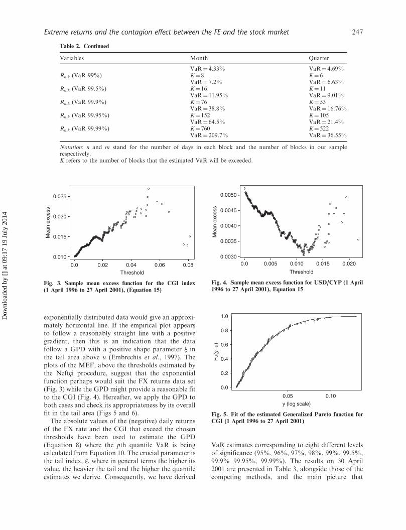
exponentially distributed data would give an approxi-mately horizontal line. If the empirical plot appearsto follow a reasonably straight line with a positivegradient, then this is an indication that the datafollow a GPD with a positive shape parameter � inthe tail area above u (Embrechts et al., 1997). Theplots of the MEF, above the thresholds estimated bythe Neftci procedure, suggest that the exponentialfunction perhaps would suit the FX returns data set(Fig. 3) while the GPD might provide a reasonable fitto the CGI (Fig. 4). Hereafter, we apply the GPD toboth cases and check its appropriateness by its overallfit in the tail area (Figs 5 and 6).

The absolute values of the (negative) daily returnsof the FX rate and the CGI that exceed the chosenthresholds have been used to estimate the GPD(Equation 8) where the pth quantile VaR is beingcalculated from Equation 10. The crucial parameter isthe tail index, �, where in general terms the higher itsvalue, the heavier the tail and the higher the quantileestimates we derive. Consequently, we have derived

VaR estimates corresponding to eight different levelsof significance (95%, 96%, 97%, 98%, 99%, 99.5%,99.9% 99.95%, 99.99%). The results on 30 April2001 are presented in Table 3, alongside those of thecompeting methods, and the main picture that

Table 2. Continued

Variables Month Quarter

VaR¼ 4.33% VaR¼ 4.69%Rn,k (VaR 99%) K¼ 8 K¼ 6

VaR¼ 7.2% VaR¼ 6.63%Rn,k (VaR 99.5%) K¼ 16 K¼ 11

VaR¼ 11.95% VaR¼ 9.01%Rn,k (VaR 99.9%) K¼ 76 K¼ 53

VaR¼ 38.8% VaR¼ 16.76%Rn,k (VaR 99.95%) K¼ 152 K¼ 105

VaR¼ 64.5% VaR¼ 21.4%Rn,k (VaR 99.99%) K¼ 760 K¼ 522

VaR¼ 209.7% VaR¼ 36.55%

Notation: n and m stand for the number of days in each block and the number of blocks in our samplerespectively.K refers to the number of blocks that the estimated VaR will be exceeded.

0.0 0.02 0.04 0.06 0.08

0.010

0.015

0.020

0.025

Threshold

Mea

n ex

cess

Fig. 3. Sample mean excess function for the CGI index

(1 April 1996 to 27 April 2001), (Equation 15)

0.0 0.005 0.010 0.015 0.0200.0030

0.0035

0.0040

0.0045

0.0050

Threshold

Mea

n ex

cess

Fig. 4. Sample mean excess function for USD/CYP (1 April

1996 to 27 April 2001), Equation 15

0.05 0.10

0.0

0.2

0.4

0.6

0.8

1.0

y (log scale)

Fu(

y–u)

Fig. 5. Fit of the estimated Generalized Pareto function for

CGI (1 April 1996 to 27 April 2001)

Extreme returns and the contagion effect between the FE and the stock market 247

Dow

nloa

ded

by [

] at

09:

17 1

9 Ju

ly 2

014

emerges is that the estimated VaRs were substantiallyhigher for the CGI returns due the higher estimatedvalue of �. We found the maximum likelihood pointestimates of � to be equal to �0.0367 for the CYP/USD rate and 0.2178 for the CGI returns while the95% confidence intervals could not exclude positivevalues for the former variable whereas the same couldnot be claimed for negative values of the latter one.7

Figures 5 and 6 depict the fit of the estimated GPDfunction for the CGI and the FX rate cases,respectively. Although the evidence from the sampleMEF suggested that we might not have beensuccessful in fitting the GPD on the FX data set,the fit of this distribution on the exceedences seemsreasonable to the naked eye. This fit is furtherinvestigated by using the crude residuals:

Wi ¼1

�log 1� �

ðYi � uÞþ

� þ �ðu� �Þ

� �ð16Þ

as defined by McNeil and Saladin (2000). Theseshould be i.i.d. unit exponentially distributed and thishypothesis can be checked by using, among othertechniques, the QQ plots of the quantiles of theexponential distribution against those of the empiricalone. Figures 7 and 8 present the diagrams for the twocases and it appears that the excesses over thethreshold are adequately modeled by the GPDfunctions since the points lie approximately along astraight line. This evidence is further supported fromthe application of the Kolmogorov–Smirnov teststatistic under which the null hypothesis that theresiduals in (16) are i.i.d. unit exponentially distributedcannot be rejected at the 1% level (the values of the teststatistics are 0.045 and 0.048 for the CGI and the FXseries respectively when the 1% critical value is 0.049).

The VaR estimates, on 30 April 2001, for all the

methods implemented, including the EVT ones, are

presented in Table 3 whereas their out-of-sample

performance is evaluated in Table 4. This evaluation is

based on one-step-ahead forecasts that have been

produced from a series of rolling samples with a size

equal to that of the initial sample (1 April 1996–

27 April 2001). Figures 9 and 10 offer a visual

presentation of the estimated VaRs (99%) with three

representative models; the GARCH(1,1), the Risk

Metrices (RM) (0.94) and the Blocks Maxima with

quarterly blocks. The main features that are worth

mentioning are that the extreme value estimates are

generally higher and they are considerably less volatile

than the other two. The rolling samples do not

generate substantial change of the data set of extreme

observations and as a result the EVT VaR estimates

are almost time independent. On the other hand, in the

GARCH–type models variances are forecasted by an

exponential model with declining weights on past

observations and therefore are crucially dependent on

the last observation that is added in the sample. The

policy suggestion of the above evidence is that the

EVT models are more suitable for long-run forecasts

of the ‘maximum’ potential losses rather than being a

day-to-day tool to measure the market risk.Various methods and tests have been suggested for

evaluating VaR model accuracy. In this article we

implement Christoffersen’s (1998) likelihood ratio

tests for coverage probability. The first one tests

whether the probability of the unconditional coverage

failure, a*, is equal to the level a selected for the VaR

calculation. Thus, the relevant null hypothesis is N0:

a*¼ a against the alternative N0: a* 6¼ a. As the

number of exceptions, x, follows a binomial distribu-

tion the likelihood ratio test statistic is:

LRuc ¼ �2 ln½ð1� aÞn�xax�

þ 2 ln½ð1� a�Þn�xða�Þx� �!

d�2ð1Þ ð17Þ

where the maximum likelihood estimator of a* is (x/n).

The second test checks whether deviations are time

dependent and the null hypothesis is that the prob-

ability of an exception occurring is independent on

what happened the day before. LRind tests for the serial

independence of the exceptions and it is defined as:

LRind ¼ �2 ln ð1� a�ÞðT00þT10Þða�ÞðT01þT11Þ �

þ 2 ln 1� a0ÞT00aT01

0 ð1� a1ÞT10aT11

1

��!d

�2ð1Þ

ð18Þ

0.009 0.020 0.030 0.040

0.0

0.2

0.4

0.6

0.8

1.0

y (log scale)

Fu(

y–u)

Fig. 6. Fit of the estimated GPD for USD/CYP (1 April

1996 to 27 April 2001)

7 The estimated values of the shape parameter � obtained from the POT and BM methods are very similar. Both indicate thatextremes from the FX rate variable could equally well be modeled by a thin-tailed distribution while the confidence intervalsfrom both models overlap.

248 S. D. Bekiros and D. A. Georgoutsos

Dow

nloa

ded

by [

] at

09:

17 1

9 Ju

ly 2

014

Tij measures the number of days in which state joccurred while it was at i the day before and ajdenotes the probability of observing an exceptionconditional on state j the previous day. If we assign

the indicators (i, j) to 0 if VaR is not exceeded and to1 otherwise then the maximum likelihood estimates ofa0 and a1 are given by (T01/(T00þT01)) and(T11/(T10þT11)) respectively. Thus, if the occurrence

Table 3. VaR (%) estimates – in absolute values – on 30 April 2001. Various methods of estimation

Percentage 95% 96% 97% 98% 99% 99.5% 99.9% 99.95% 99.99%

CYP/USDRM(0.94) 1.48 1.58 1.70 1.85 2.10 2.32 2.79 2.97 3.35MA(20) 1.49 1.58 1.70 1.86 2.11 2.33 2.80 2.98 3.37MA(60) 1.58 1.69 1.81 1.98 2.24 2.48 2.98 3.17 3.58GARCH(GED) 1.56 1.66 1.78 1.94 2.20 2.44 2.93 3.12 3.52GARCH(N) 1.58 1.69 1.81 1.98 2.24 2.48 2.98 3.17 3.58GARCH(t) 1.57 1.67 1.80 1.96 2.22 2.46 2.95 3.14 3.55HS 1.14 1.22 1.30 1.41 1.61 1.88 2.53 2.60 2.66MC-RM(0.94) 1.47 1.62 1.73 1.90 2.15 2.29 2.90 2.97 3.03MC-MA(60) 1.61 1.67 1.79 1.97 2.09 2.22 2.48 2.49 2.49MC-GARCH(GED) 1.54 1.58 1.69 1.90 2.25 2.48 2.57 2.74 2.87MC-GARCH(N) 1.52 1.68 1.79 1.96 2.16 2.32 2.75 2.92 3.05MC-GARCH(t) 1.51 1.59 1.77 1.92 2.19 2.52 3.11 3.31 3.48EVT-POT 1.13 1.21 1.31 1.45 1.69 1.92 2.43 2.64 3.11EVT-BM(60) 1.08 1.17 1.28 1.45 1.73 2.01 2.69 2.99 3.70

CGIRM(0.94) 2.85 3.03 3.25 3.55 4.03 4.46 5.35 5.69 6.44MA(20) 2.65 2.82 3.03 3.31 3.75 4.16 4.98 5.31 6.00MA(60) 2.85 3.04 3.26 3.56 4.03 4.47 5.36 5.71 6.45GARCH(GED) 3.36 3.57 3.84 4.19 4.75 5.26 6.31 6.72 7.59GARCH(N) 3.29 3.50 3.76 4.10 4.65 5.15 6.18 6.58 7.43GARCH(t) 3.40 3.62 3.89 4.25 4.81 5.33 6.39 6.80 7.69HS 2.39 2.69 3.02 3.65 4.96 6.34 9.56 9.94 10.05MC-RM(0.94) 2.92 3.07 3.28 3.78 4.18 4.41 5.10 5.94 6.62MC-MA(60) 2.85 3.06 3.30 3.55 3.94 4.46 4.63 4.69 4.74MC-GARCH(GED) 3.13 3.36 3.56 4.00 4.42 4.79 5.48 5.85 6.15MC-GARCH(N) 3.32 3.44 3.70 3.92 4.29 4.73 5.32 5.75 6.10MC-GARCH(t) 3.42 3.58 3.85 4.17 4.56 5.31 6.70 6.82 6.92EVT-POT 2.38 2.69 3.11 3.73 4.89 6.18 9.79 11.66 16.87EVT-BM(60) 2.63 3.09 3.71 4.69 6.63 9.01 16.76 21.4 36.55

Notation: RM¼Riskmetrics, MA(60)¼ 60 days moving average, GED¼Generalized Error Distribution, MC¼Monte-Carlo, HS¼Historical Simulation, POT¼Peaks-over-Threshold, BM(60)¼ 60 days blocks.

0 2 4

0

1

2

3

4

5

Ordered quantiles

Exp

onen

tial q

uant

iles

1 3 5

Fig. 8. QQ Plot of residuals from the fitted GPD (1 April

1996 to 27 April 2001) against the exponential distribution

(USD/CYP), (Equation 16)

0 2 4

0

1

2

3

4

5

Ordered quantiles

Exp

onen

tial q

uant

iles

1 3

Fig. 7. QQ Plot of residuals from the fitted GPD (1 April

1996 to 27 April 2001) against the exponential distribution

(CGI), (Equation 16)

Extreme returns and the contagion effect between the FE and the stock market 249

Dow

nloa

ded

by [

] at

09:

17 1

9 Ju

ly 2

014

Table 4. Number of exceedances, F, and 95% LRuc nonrejection test confidence regions (Equation 17). Backtesting sample

period: 30 April 2001 to 19 April 2002 (255 observations)

Percentage 95% 96% 97% 98% 99% 99.5% 99.9% 99.95% 99.99%

Failures (LRuc) 6<F<21 4<F<17 2<F<14 1<F<11 F<7 F<5 F<2 F<2 F<1

CYP/USDRM(0.94) 14 11 9 6 5 4 2 2 1MA(20) 14 12 9 7 4 4 2 2 1MA(60) 15 11 7 5 4 3 2 1 0GARCH(GED) 15 13 8 5 4 3 2 1 0GARCH(N) 15 13 7 5 4 3 2 1 0GARCH(t) 15 13 7 5 4 3 2 1 0HS 23 20 18 13 7 3 1 1 1MC-RM(0.94) 14 13 9 7 5 4 3 3 2MC-MA(60) 16 12 8 5 5 4 2 2 2MC-GARCH(GED) 16 13 9 5 4 3 2 2 2MC-GARCH(N) 16 12 10 5 4 2 1 1 1MC-GARCH(t) 16 15 10 6 4 4 2 1 1EVT-POT 23 21 17 12 6 3 1 1 1EVT-BM(60) 24 23 22 15 5 3 1 1 1

CGIRM(0.94) 19 12 11 9 4 2 1 1 1MA(20) 22 18 16 11 5 3 2 2 2MA(60) 12 9 9 8 5 3 2 2 1GARCH(GED) 22 19 14 13 8 7 4 4 1GARCH(N) 19 13 9 8 6 5 2 1 1GARCH(t) 22 19 14 13 9 7 4 4 1HS 18 14 11 5 3 2 0 0 0MC-RM(0.94) 17 12 11 9 5 4 1 1 1MC-MA(60) 11 10 10 9 5 4 2 2 1MC-GARCH(GED) 24 18 16 13 9 7 5 3 3MC-GARCH(N) 19 14 9 8 6 5 4 2 2MC-GARCH(t) 21 18 18 12 10 7 5 5 1EVT-POT 15 13 9 4 3 2 0 0 0EVT-BM(60) 17 10 6 3 2 1 0 0 0

Notes: Numbers in italics indicate, statistically significant, overestimation or underestimation of risk. F is the number offailures that could be observed without rejecting the null that the models are correctly calibrated at the 95% level ofconfidence.

−0.06

−0.04

−0.02

0

0.02

0.04

0.06

0.08

0.1

0.12

0.14

1 51 101 151 201 251

Returns GARCH(1,1) RM(0.94) EVT-BM(60)

Fig. 9. CGI returns, negated and VaR (99%) estimates (30 April 2001 to 19 April 2002)

250 S. D. Bekiros and D. A. Georgoutsos

Dow

nloa

ded

by [

] at

09:

17 1

9 Ju

ly 2

014

of an exception is independent of previous day’s

conditions then a¼ a0¼ a1¼ (T01þT11)/T) and LRind

should not be statistically significant. By combining

the two tests, a third test of conditional coverage,

LRcc, can be constructed as:

LRcc ¼ LRuc þ LRind �!d

�2ð2Þ ð19Þ

In Table 4 we present the number of exceedances as

well as the confidence regions of failures that are

implied from Christoffersen’s (1998) likelihood ratio

tests. The main evidence is that for the FX rate return

series, which does not exhibit a strong fat tails

behaviour, the EVT does not perform well at

conventional levels of significance, up to 98%, and

there are other methods that provide consistentlymore accurate estimates of the maximum loss (e.g. themoving average and the GARCH type models). It isonly at levels of significance higher than 99% that theEVT methods produce a prediction success ratesimilar to that of the other methods. However,these results are reversed when we look at the stockmarket index returns that exhibit clearly a fat tailsbehaviour. Here, the superiority of the EVT techni-ques at high levels of significance, in terms of theaccuracy of the estimates of maximum losses, isclearly evident.

Finally, in Fig. 11 we present the predicted one-dayahead correlation index of extreme returns that isbased on the estimation of the coefficient a from the

−0.3

−0.2

−0.1

0

0.1

0.2

0.3

0.4

0.5

12/4/2001 12/6/2001 12/8/2001 12/10/2001 12/12/2001 12/2/2002 12/4/2002

DatesRM094

Cor

rela

tion

coef

ficie

nt

EVT-POT GARCH(N)

Fig. 11. Forecasted correlation for CYP/USD vs. CGI returns (30 April 2001 to 19 April 2002)

−0.03

−0.02

−0.01

0

0.01

0.02

0.03

0.04

1 51 101 151 201 251

Returns GARCH(1,1) RM(0.94) EVT-BM(60)

Fig. 10. USD/CYP returns, negated and VaR (99%) estimates (30 April 2001 to 19 April 2002)

Extreme returns and the contagion effect between the FE and the stock market 251

Dow

nloa

ded

by [

] at

09:

17 1

9 Ju

ly 2

014

Tiago de Oliveira (1973) formula. For comparisonreasons we have also estimated the correspondingcorrelation index by fitting a bivariate GARCHmodel where the variance and covariance equationsare modeled as GARCH(1,1) processes. As a sub-casewe also consider the restricted bivariate GARCH asimplied by the RM(0.94) specification. The obtainedvalues of the correlation index from the bivariateEVT are around 0.2 when the GARCH(1,1) methodgives estimates close to zero and the RM(0.94)extremely volatile estimates which however averageto zero as well.8 The evidence suggests that there hasbeen a very low correlation between exchange rateand the stock market daily returns in Cyprus. Thisconclusion holds even at crises periods since thecorrelation coefficient of extremes retains values closeto 0.20. Another interesting result is that the bearmarket conditions that characterize the backtestingperiod do not appear to have affected the extremecorrelation index.

The reasons for those findings can be traced to thecapital controls that restricted short-term borrowingby residents, the intervention policy of the centralbank of Cyprus as well as to the fact that thebubble in the Cyprus Stock exchange was mainlydomestically driven.

IV. Concluding Remarks

In this article we have applied the univariate andmultivariate EVT in order to derive different VaRestimates for two inherently unstable markets; theforeign exchange and the stock market. Theseestimates are compared to those obtained frommore ‘traditional’ methods of estimation through abacktesting exercise. The data for this exercise consistof the daily returns of the US dollar/Cyprus poundexchange rate and the CGI. The main conclusion wehave reached is that for a return series that is heavytailed distributed, i.e. the stock market returns in ourcase, the extreme value techniques give more accurateloss prediction results. However, this result is reversedif one attempts to apply this methodology on a seriesthat might not exhibit strong ‘fat’ tails characteristics,i.e. the foreign exchange returns in our case. We havealso derived estimates of the correlation index of theextreme observations of those two markets and weobtained substantial differences from the competingmodels. The main result here is that the correlation ofextreme returns between the Cyprus pound/USD

exchange rate and the Cyprus General Index dailyreturns is quite low but clearly higher than the onethat is based on the entire sample of observations.

References

Adler, M. and Dumas, B. (1983) International portfolioselection and corporate finance: a synthesis, Journal ofFinance, 38, 925–84.

Ajayi, R. A. and Mougoue, M. (1996) On the dynamicrelation between stock prices and exchange rates, TheJournal of Financial Research, 2, 193–207.

Akgiray, V. and Booth, G. G. (1988) The stable-law modelof stock returns, Journal of Business and EconomicStatistics, 6, 51–7.

Alexander, C. (1998) Volatility and correlation: measure-ment, models and applications, in Risk Managementand Analysis: Measuring and Modelling Financial Risk(Ed.) C. Alexander, J. Wiley & Sons, Wiley,pp. 125–72.

Artzner, R, Delbaen, F., Eber, J.-M. and Heath, D. (1999)Coherent measures of risk, Mathematical Finance, 9,203–28.

Balkema, A. and de Haan, L. (1974) Residual life time atgreat age, Annals of Probability, 2, 792–804.

Blattberg, R. C. and Gonedes, N. (1974) A comparison ofthe stable and student distributions as statisticalmodels for stock prices, Journal of Business, 47,244–80.

Boyer, B., Gibson, M. and Loretan, M. (1999) Pitfalls intests for changes in correlations, International FinanceDiscussion Papers No 597. Board of Governors of theFederal Reserve System, Washington.

Campbell, J., Lo, A. W. and MacKinlay, A. C. (1997) TheEconometrics of Financial Markets, PrincetonUniversity Press.

Christoffersen, P. (1998) Evaluating interval forecasts,International Economic Review, 39, 841–62.

Cox, D. and Snell, E. (1968) A general definition ofresiduals (with discussion), Journal of the RoyalStatistical Society, 30, 248–75.

de Haan, L. (1976) Sample extremes: an Introduction,Statistica Neerlandica, 30, 161–72.

Embrechts, P., Kluppelberg, C. and Mikosch, T. (1997)Modelling Extremal Events for Insurance and Finance,Springer, Berlin.

Fisher, R. and Tippet, L. (1928) Limiting forms of thefrequency distribution of the largest or smallestmember of a sample, Proceedings of the CambridgePhilosophical Society, 24, 180–90.

Gencay, R. and Selcuk, F. (2004) Extreme value theory andvalue-at-risk: relative performance in emerging mar-kets, International Journal of Forecasting, 20, 287–303.

Grauer, F., Litzenberger, R. and Stehle, R. (1976) Sharingrules and equilibrium in a international capital marketunder uncertainty, Journal of Financial Economics, 3,233–56.

Harvey, C., Solnik, B. and Zhou, G. (2002) Whatdetermines expected international asset returns?,Annals of Economics and Finance, 3, 249–98.

8 The extremely volatile estimates of the conditional correlation under the RM approach, in Fig. 11, is due to the fact that theestimated decay factor, 1, of Equation A7, in the appendix, is higher under the GARCH (1,1) model.

252 S. D. Bekiros and D. A. Georgoutsos

Dow

nloa

ded

by [

] at

09:

17 1

9 Ju

ly 2

014

Jansen, D. and de Vries, G. (1991) On the frequency oflarge stock returns: putting booms and busts intoperspective, The Review of Economics and Statistics,73, 18–24.

Jenkinson, A. F. (1955) Distribution of the annualmaximum (or minimum) values of meteorologicalelements, Quarterly Journal of Royal MeteorologicalSociety, 81, 141–58.

Krugman, P. (1995) Dutch tulips and emerging markets,Foreign Affairs, 74, 28–44.

Leadbetter, M., Lindgren, G. and Rootzen, H. (1983)Extremes and related properties of random sequencesand processes, Springer, Berlin.

Longin, F. (2000) From value at risk to stress testing: theextreme value approach, The Journal of Banking andFinance, 24, 1097–130.

Longin, F. and Solnik, B. (2001) Extreme correlation ofinternational equity markets, The Journal of Finance.,2, 649–76.

McNeil, A. (1998) Calculating Quantile Risk Measures forFinancial Return Series using Extreme Value Theory,Preprint, ETH Zurich.

McNeil, A. and Saladin, T. (2000) Developing scenarios forfuture extreme losses using the POT method,in Extremes and Integrated Risk Management (Ed.)P. Embrechts, RISK books, London.

Neftci, S. (2000) Value at risk calculations, extreme events,and tail estimation, Journal of Derivatives, 7, 23–38.

Nerouppos, M., Saunders, D., Xiouros, C. and Zenios,S. (2002) The Risks of the Cyprus and Athens

Stock Exchange, HERMES Center ofExcellence on Computational Finance andEconomics, University of Cyprus, WorkingPaper 02–5.

Pickands, J. (1975) Statistical inference usingextreme order statistics, The Annals of Statistics, 3,119–31.

Singh, A. and Weisse, B. (1998) Emerging stock markets,portfolio capital flows and long-term economicgrowth: micro and macroeconomic perspectives,World Development, 26, 607–22.

Sklar, A. (1959) Fonctions de repartition a n dimensions etleurs marges, Publications de l’Institut de Statistique del’Universite de Paris, 8, 229–31.

Smith, R. (1987) Estimating tails of probability distribu-tions, Ann. Statis., 15, 1174–207.

Smith, R. and Weissman, I. (1994) Estimating the extremalindex, Journal of the Royal Statistical Society, 56,515–28.

Solnik, B. (1983) International arbitrage pricing theory,Journal of Finance, 38, 449–57.

Tawn, J. A. (1988) Bivariate extreme value theory,Biometrica, 75, 397–415.

Tiago de Oliveira, J. (1973) Statistical Extremes – A Survey,Center of Applied Mathematics, Lisbon.

Tirole, J. (1991) Privatisation in Eastern Europe: Incentivesand the Economics of Transition, in NBERMacroeconomics Annual 1992 (Eds) O. J. Blanchardand S. Fischer, NBER Macroeconomic Annual, TheMIT Press, Cambrige.

Appendix A. Conventional methods forthe Estimation of the VaR and theCorrelation Index

Let ðYtÞnt¼1 represent identically and

independently distributed, i.i.d., daily returns of a

financial asset price. We can then define VaRt(a), as

the conditional on the information set, Tt�1, �thquantile, i.e.

PrYt � VaRtðaÞ

It�1

� �¼ a ðA1Þ

Suppose now that ðYtÞnt¼1 follows the stochastic

process:

Yt ¼ �t þ et ¼ �t þ �t"t ðA2Þ

where �t ¼ EðYt=It�1Þ, �2t ¼ Eðe2t =It�1Þ and "t¼ (et/�t)

has the conditional distribution function �t(�).

Under the parametric approach we consider

specific distributions for �t(�) such as the Gaussian

N(0,1), the Student-t and the GED. Therefore,

VaRt(a) is estimated by inverting the distribution

function:

VaRtðaÞ ¼ �t þ��1t ðaÞ�t ðA3Þ

The conditional variance can be estimated by various

volatility models such as the moving average, MA,

variance or alternatively by one of the family of

GARCH models. In particular, the standard

GARCH(1,1) model is given by:

�2t ¼ �0 þ �1ðYt�1 � �tÞ

2þ �2

t�1 ðA4Þ

where �t ¼ ð1=TÞPT

i¼1 Yt�i. As a special case we will

be concerned with the EWMA specification, adopted

by the (RM) model of J. P. Morgan, under which:

�2t ¼ ��2

t�1 þ ð1� �ÞðYt�1 � �tÞ2

ðA5Þ

Riskmetrics has chosen �¼ 0.94 and �¼ 0.97 as the

optimal decay factor for daily and monthly data,

respectively.The second methodology we explored was based

on nonparametric approaches to model the distribu-

tion of returns. Historical simulation makes use of the

empirical quantiles of returns to estimate VaRs for a

given confidence level. The critical assumption behind

this approach is that the historical distribution of

returns will remain the same over the next periods.

Also, a feature of this method is that extrapolation

beyond past observations is impossible and therefore

extreme quantiles cannot be estimated. If a long

sample is chosen instead, then the method is unable to

Extreme returns and the contagion effect between the FE and the stock market 253

Dow

nloa

ded

by [

] at

09:

17 1

9 Ju

ly 2

014

distinguish between high and low volatility periodsand as a result it might generate inaccurate estimates.

With the Monte Carlo, MC, simulation methodone simulates the future value of an asset based on anunderlying stochastic process. In this article theBrownian motion process, in its discrete time version,has been adopted for the asset price S, that is:

�St

St�1¼ Yt ¼ �t�t�tþ �t�1"t

ffiffiffiffiffiffi�t

p� ðA6Þ

where "t, is a zero mean, unit variance error term, and�t and �t are drift and volatility parameters. In theempirical investigation we have allowed for a possibletime-varying volatility structure where the volatilitycoefficient is being estimated by GARCH-normal,GARCH-t, GARCH-GED, RM(0.94) and MA(60).

In order to estimate the conditional correlationwith the ‘conventional’ approaches a bivariateGARCH model has been fitted to the data(Alexander, 1998). The specification of the model is

given by the conditional mean Equations A2 for eachone of the two variables Y1,t and Y2,t and thefollowing conditional variance and covariance equa-tions which are modeled as GARCH(1,1) processes invech parameterization:

h21, t ¼ �0 þ �1e21, t�1 þ �2h

21, t�1

h22, t ¼ 0 þ 1e22, t�1 þ 2h

22, t�1

h12, t ¼ 0 þ 1h12, t�1 þ 2ðY1, t�1 � �1, t�1Þ

� ðY2, t�1 � �2, t�1Þ

ðA7Þ

Under the Riskmetrics approach the followingparameter values apply: 0¼ 0, 1¼ 0.94, 2¼ 0.06.The conditional correlation is then given by:

�t ¼h12, t

h1, th2, tðA8Þ

254 S. D. Bekiros and D. A. Georgoutsos

Dow

nloa

ded

by [

] at

09:

17 1

9 Ju

ly 2

014