Extraction of tool reaction forces using LS- DYNA and its ...

Faculty of Engineering, Blekinge Institute of Technology, 371 79 Karlskrona, Sweden

Master of Science in Mechanical Engineering February 2019

Extraction of tool reaction forces using LS-DYNA and its use in Autoform sheet metal

forming simulation

Esbjörn Zachén

This thesis is submitted to the Faculty of Engineering at Blekinge Institute of Technology in partial fulfilment of the requirements for the degree of Master of Science in Mechanical Engineering. The thesis is equivalent to 20 weeks of full time studies. The authors declare that they are the sole authors of this thesis and that they have not used any sources other than those listed in the bibliography and identified as references. They further declare that they have not submitted this thesis at any other institution to obtain a degree.

Contact Information: Author: Esbjörn Zachén E-mail: [email protected]

University advisor: Mats Walter Department of Mechanical Engineering

Faculty of Engineering Blekinge Institute of Technology SE-371 79 Karlskrona, Sweden

Internet : www.bth.se Phone : +46 455 38 50 00 Fax : +46 455 38 50 57

i

ABSTRACT In product development there is still potential to decrease lead times with faster and more accurate simulations. The objective of this thesis was to study whether Finite Element (FE) simulations using explicit LS-DYNA to extract reaction forces from sheet metal forming tools during forming, could be used to improve existing FE models in sheet metal forming software AutoForm. To begin with, the solid CAD-model of the stamping dies were meshed with tetrahedral elements in CATIA and imported into LS-DYNA. In combination with sheet mesh and milling surface meshes from AutoForm, an explicit model was realized. Contacts between sheet mesh and milling surface meshes used the so-called sheet forming contact. The resulting reaction forces were extracted and used in a simulation using the AutoForm software. Resulting simulation was compared to a scan of the physical sheet metal after forming. The direct transfer of reaction forces from LS-DYNA to AutoForm did however not result in the same pressure distribution in AutoForm. The AutoForm simulations using results from LS-DYNA were slightly worse than standard AutoForm simulations. Further work is needed to try and perhaps implement an implicit solution after an initial explicit solution. Keywords: Sheet Metal Forming, Stamping Die, blank holder, Structural Analysis, Finite Element Simulation

ii

SAMMANFATTNING Inom produktutveckling finns möjligheter att förkorta ledtider genom snabbare och mera korrekta simuleringar. Syftet med detta arbetet var att undersöka huruvida resultat från explicit LS-DYNA kunde användas för att förbättra nuvarande plåtformningssimuleringar i AutoForm. Den solida CAD-modellen av verktyget meshades med tetraediska element i CATIA och importerades till LS-PrePost, tillsammans med fräsytsmeshar och plåtmesh från AutoForm. Kontakter etablerades mellan plåt och fräsytsmeshar med så kallad sheet forming contact. Modellen löstes sedan explicit. Resulterande reaktionskrafter på plåthållare exporterades till AutoForm och implementerades där. Resulterande simulering jämfördes mot en inskannad fysisk plåt efter plåtformning. Direkt implementering av reaktionskrafter på plåthållaren i AutoForm gav resultat som avvek mer mot inskannad plåt än nuvarande simuleringsstrategi. Direkt implementering av reaktionskrafter gav heller inte en tryckfördelning som liknade den som rapporterades av LS-DYNA. Mer arbete krävs för att om möjligt implementera en implicit lösning efter en initial explicit lösning.

iii

ACKNOWLEDGEMENT Advice, ideas, and support by my co-advisor Mats Sigvant have been critical for the completion of this project. I would like to offer my special thanks to Johan Pilthammar for valuable support on the proper commands to use with the LS-DYNA compute server, examining meshes, and setting up and running extra simulations. I would also like to thank Volvo Cars for providing the necessary software, hardware and compute capabilities, as well as a comfy place to work at Volvo Cars in Olofström. Further I would also like to thank Mikael Schill at Dynamore Sweden for his assistance in answering our questions on settings and usage of the LS-PrePost software.

iv

NOMENCLATURE ACRONYMS

CAD Computer Aided Design FEM Finite Element Method IGES Initial Graphics Exchange Specification (for CAD data exchange)

SMF Sheet Metal Forming TRL Technology Readiness Level

v

TABLE OF CONTENTS ABSTRACT ............................................................................................................................................................ I

SAMMANFATTNING ........................................................................................................................................ II

ACKNOWLEDGEMENT .................................................................................................................................. III

NOMENCLATURE ............................................................................................................................................ IV

TABLE OF CONTENTS ...................................................................................................................................... V

TABLE OF FIGURES ....................................................................................................................................... VII

1 INTRODUCTION .........................................................................................................................................1

1.1 AIM AND THESIS QUESTIONS ..................................................................................................................2 1.2 LIMITATIONS OF WORK ............................................................................................................................2 1.3 ETHICS, SOCIETY AND SUSTAINABILITY ..................................................................................................2 1.4 THEORETICAL FRAMEWORK ....................................................................................................................3

1.4.1 Sheet metal forming ............................................................................................................................3 1.4.1.1 Deep drawing ........................................................................................................................................... 3 1.4.1.2 Stretch forming ......................................................................................................................................... 3 1.4.1.3 Combined deep drawing and stretch forming ........................................................................................... 3

1.4.2 Simulation evaluation techniques .......................................................................................................4 1.4.3 Finite Element Method .......................................................................................................................5

1.4.3.1 Introduction .............................................................................................................................................. 5 1.4.3.2 Elements ................................................................................................................................................... 5 1.4.3.3 Boundary Conditions ................................................................................................................................ 6 1.4.3.4 Symmetry ................................................................................................................................................. 7

1.4.4 Software used .....................................................................................................................................7 1.4.4.1 CATIA ...................................................................................................................................................... 7 1.4.4.2 LS-DYNA ................................................................................................................................................ 7 1.4.4.3 LS-PrePost ................................................................................................................................................ 7 1.4.4.4 AutoForm ................................................................................................................................................. 8 1.4.4.5 GOM Inspect ............................................................................................................................................ 8 1.4.4.6 MATLAB ................................................................................................................................................. 8

1.4.5 Blank holder load modelling in a single action press ........................................................................8 1.4.6 LS-DYNA Energy Ratio ......................................................................................................................8 1.4.7 Software Parameters ..........................................................................................................................9

1.4.7.1 SHRF ........................................................................................................................................................ 9 1.4.7.2 NIP ........................................................................................................................................................... 9 1.4.7.3 PARMAX / MAXPAR ............................................................................................................................. 9 1.4.7.4 Sag .......................................................................................................................................................... 10

2 RELATED WORK ..................................................................................................................................... 11

3 METHODS .................................................................................................................................................. 12

3.1 DEVELOPMENT METHOD........................................................................................................................ 12 3.1.1 Main method description .................................................................................................................. 12 3.1.2 Secondary methods description and usage....................................................................................... 13

3.1.2.1 Literature review .................................................................................................................................... 13 3.1.2.2 Gathering data from the customers ......................................................................................................... 13

3.1.3 Method argumentation ..................................................................................................................... 13 3.1.3.1 Simulation .............................................................................................................................................. 13 3.1.3.2 Literature review .................................................................................................................................... 14 3.1.3.3 Gathering data from the customers ......................................................................................................... 14

3.1.4 Limits and threats to validity of methods ......................................................................................... 14 3.1.4.1 Simulation .............................................................................................................................................. 14 3.1.4.2 Literature review .................................................................................................................................... 14 3.1.4.3 Gathering data from the customers ......................................................................................................... 14

3.1.5 Choice of tools for conducting simulations ...................................................................................... 15 3.2 GENERAL LS-DYNA SETTINGS ............................................................................................................ 15

vi

3.2.1.1 Consistent units ...................................................................................................................................... 15 3.2.1.2 Mass scaling ........................................................................................................................................... 15

3.3 MODEL CREATION................................................................................................................................. 16 3.3.1 Meshing ............................................................................................................................................ 16

3.3.1.1 Solid tools ............................................................................................................................................... 16 3.3.1.2 Pins ......................................................................................................................................................... 16 3.3.1.3 Sheet Metal ............................................................................................................................................. 16 3.3.1.4 Die milling surface ................................................................................................................................. 16

3.3.2 Material properties and element types ............................................................................................. 17 3.3.3 Boundary conditions, contacts and loading ..................................................................................... 17 3.3.4 Contact definitions ........................................................................................................................... 19

3.4 GOM INSPECT COMPARISON CREATION ................................................................................................ 19

4 RESULTS ..................................................................................................................................................... 20

4.1 REACTION FORCES ON PINS ................................................................................................................... 20 4.2 PRESSURE DISTRIBUTION ....................................................................................................................... 22 4.3 AUTOFORM IMPLEMENTATION .............................................................................................................. 22

4.3.1 AutoForm pressure distribution ....................................................................................................... 22 4.3.2 AutoForm complete sheet forming ................................................................................................... 23

4.4 SIMULATION GUIDELINES ...................................................................................................................... 24

5 ANALYSIS AND DISCUSSION ................................................................................................................ 25


5.3.1 AutoForm pressure distribution vs LS-DYNA .................................................................................. 26 5.3.2 AutoForm complete sheet forming ................................................................................................... 27

5.4 VARIOUS ITEMS ..................................................................................................................................... 28 5.4.1 General behavior of model throughout the simulation .................................................................... 29 5.4.2 Energy Ratio..................................................................................................................................... 29 5.4.3 Sensitivity to mass scaling ................................................................................................................ 29 5.4.4 Frequency response of the system .................................................................................................... 29 5.4.5 Rigid behavior of top of upper matrix .............................................................................................. 30 5.4.6 Load curve shape dependency .......................................................................................................... 31 5.4.7 Pressure values compared to AutoForm .......................................................................................... 31

6 CONCLUSION ............................................................................................................................................ 33


6.3.1 Autoform pressure distribution vs LS-DYNA ................................................................................... 33 6.3.2 Autoform complete sheet forming ..................................................................................................... 33

6.4 RESEARCH QUESTION ............................................................................................................................ 33

7 FUTURE WORK ........................................................................................................................................ 34

7.1 CONTACT PRESSURE TRANSFER TO AUTOFORM .................................................................................... 34 7.2 CONTACT PRESSURE ADJUSTMENT IN LS-DYNA .................................................................................... 34 7.3 IMPLICIT ANALYSIS IMPLEMENTATION .................................................................................................. 34

REFERENCES ..................................................................................................................................................... 35

vii

TABLE OF FIGURES Figure 1 Rigid die and press during SMF ............................................................................................... 1 Figure 2 Traditional die manufacturing process ...................................................................................... 1 Figure 3 Schematic illustration of the deep drawing and stretch forming process .................................. 3 Figure 4 Schematic of Mechanical double-action press .......................................................................... 4 Figure 5 Hydraulic single action press .................................................................................................... 4 Figure 6 Illustration of the modelling steps using Finite Element Analysis ........................................... 5 Figure 7 A four-node tetrahedral element (left) and a ten-node tetrahedral (right) ................................. 6 Figure 8 Sag reduction by mesh refinement ............................................................................................ 6 Figure 9 3D modelling vs 2D axisymmetric modelling .......................................................................... 7 Figure 10 Cross cut of shell with 5 point through thickness gauss integration ....................................... 9 Figure 11 MAXPAR 1.0 and 1.2 ............................................................................................................. 9 Figure 12 Common steps in simulation methodology ........................................................................... 12 Figure 13 Overview of the Second Model ............................................................................................ 15 Figure 14 Original Pin geometry meshed with 20 to 10 mm elements (left) Modified Pin (right) not to

scale, 48 is the number of pins ...................................................................................................... 16 Figure 15 Unstable behavior ................................................................................................................. 17 Figure 16 Unstable behavior ................................................................................................................. 17 Figure 17 Boundary Conditions for blank holder, X and Y direction ................................................... 18 Figure 18 Upper Matrix with nodes locked in X and Y direction, as well as all rotations highlighted 18 Figure 19 Pins with bottom nodes locked for all DOFs ........................................................................ 18 Figure 20 Light Yellow (Solid) Dark Yellow (blank holder milling surface mesh) ............................. 19 Figure 21 Reaction forces on pins ......................................................................................................... 20 Figure 22 Extracted pin reaction forces and pin numbering ................................................................. 20 Figure 23 Sum of Reaction forces from all pins (fs = 10kHz) .............................................................. 21 Figure 24 Handpicked vs filtered values, Pins No 1-24 ........................................................................ 21 Figure 25 Pressure distribution on sheet metal...................................................................................... 22 Figure 26 Short edge pressure distribution ............................................................................................ 22 Figure 27 AutoForm blank holder pressure distribution using LS-DYNA forces ................................ 23 Figure 28 AutoForm blank holder pressure distribution using standard simulation ............................. 23 Figure 29 Allact6 Standard simulation surface deviation to scanned sheet metal ................................ 24 Figure 30 Allact6 Simulation with forces extracted from LS-DYNA, surface deviation to scanned sheet

metal .............................................................................................................................................. 24 Figure 31 Distribution of total reaction force on single pin (Pins 1-24) ............................................... 25 Figure 32 Initial pressure distribution, beads to sheet metal (Left) Improved pressure distribution beads

to sheet metal (Right) .................................................................................................................... 26 Figure 33 Pressure Distribution in LS-DYNA ...................................................................................... 27 Figure 34 Pressure distribution in AutoForm using extracted LS-DYNA forces ................................. 27 Figure 35 Pressure distribution in AutoForm using standard simulation .............................................. 27 Figure 36 Standard simulation .............................................................................................................. 28 Figure 37 Using extracted LS-DYNA forces ........................................................................................ 28 Figure 38 Sum of reaction forces over time .......................................................................................... 30 Figure 39 Nodal displacement upper matrix ......................................................................................... 31 Figure 40 Load Curve comparison ........................................................................................................ 31 Figure 41 Change in energy ratio, Smooth vs Ramped ......................................................................... 31

1

1 INTRODUCTION The introductory chapter is presented to give the readers an introduction to the studied subject and in hopes of helping readers understand the reasons for choices made in the thesis as well as a better understanding of the thesis. An important process when constructing cars is the sheet metal forming (SMF) process [1]. This process is used to create body components such as doors, hoods and beams[1]. The sheet metal is formed in dies which are mounted in stamping presses[1]. A schematic overview of the stamping process can be seen in Figure 1. Simulation of the SMF process has been done for many years, the simulations can predict the final shape, tearing, wrinkles, thickness and strains among other things with various accuracy, see Pilthammar [1].

Figure 1 Rigid die and press during SMF

Designing and manufacturing stamping dies is a costly part of a new vehicle[1]. Traditionally the process is initially done virtually and later physically, displayed in Figure 2[1]. In the die manufacturing process, the die is cast, left to cool for three weeks, and then machined to specifications[1]. During the manual rework the tool is first in try out in the tool shop with its own press, later the die is moved to the production facilities and further manual rework is usually needed until it gives satisfactory results[1]. The manual rework consists of adding or removing material to/from the forming surfaces of the die with the help of welding, milling or grinding[1]. This process can take up to five weeks[1].

Figure 2 Traditional die manufacturing process

In the production of formed sheet metal, it is important to reduce the time from an idea to a finished product. One way of decreasing this lead time, is to have even more accurate simulation models so that less iterations are needed. The requirements on models for predicting forming of sheet metal is also increasing due to demands on smaller tolerances, reduced scrap and higher quality products[1]. Traditionally the SMF simulation is done with the assumption that the dies and the press is rigid[1]. This is mostly since incorporation of elastic dies and press structures lead to very high computational costs, and partly it depends on where in the process the simulation is taking place[1]. Early on the surrounding tools have not been designed and can therefore not be included any way[1]. Since the die needs to cool for three weeks before it is milled to specification a window of opportunity for including elastic die geometry in the SMF simulation is open[2]. In this timeframe it would be possible to simulate and assess the influence of the die and press deformations and the resulting reaction forces, and if they can be solved simply by slight modifications to the milling surfaces[2]. In this thesis, the aim is to extract blank

2

holder reaction forces and implement them into today’s metal forming software (namely AutoForm) used by Volvo Cars. Volvo Cars started producing automobiles in Sweden in 1927. Today Volvo Cars is a global company with sales in about 100 countries. The company headquarter is in Sweden, additionally there are manufacturing plants in Sweden, Belgium, USA and China[3]. This thesis was primarily conducted at Volvo Cars Body Components located in Olofström Sweden where body components for automobiles are pressed and partly assembled[2].

1.1 Aim and thesis questions The content of this chapter is presented to clarify the specific research question asked by this thesis. The choice of research question was based on an interview with Mats Sigvant where it was proposed by Mats Sigvant[2]. The author chose to work on this research question due to that it appeared the most interesting to him personally among the multitude of alternatives discussed with Mats Sigvant. As an overall goal for this thesis one might set “Better knowledge in sheet metal forming simulation for shorter lead time in sheet metal forming development”.

Research question:

• Will physically more correct modelling of blank holder load lead to simulations that markedly agree better with available measurements?

Stake holders that may be interested include all sheet metal manufacturers using small dies in large double action presses. This work should clarify how one can determine the force that is applied on each blank holder pin. Another goal is to provide simulation guidelines for the kind of simulation done in this thesis.

1.2 Limitations of work The contents of this chapter are presented to show that the author has made some effort to try and limit the extent to which the work is carried out. Software will not be developed to plugin fidelity as for example the TriboForm software. This was based on the assumption that reaching a plugin fidelity is a time-consuming endeavor. There will not be enough time or money to test physical solutions to single action press pin contact pressure. The author has limited experience in creating physical models and a physical model that would give answers with enough fidelity to compare with simulation results was thought to be costly and time consuming [4]. In hindsight one should perhaps have at least tried to spend one or two days to create a cheap physical model and see how good results it would give.

1.3 Ethics, Society and Sustainability The contents of this chapter are presented to show readers the possible implications of this thesis on ethical, societal and sustainability issues. Humans and or animals will not be investigated in this thesis, therefore ethical aspects are deemed irrelevant for this work. Societal aspects might be invoked since improved models leads to less problems in production and thereby limiting the number of times the personnel at the manufacturing site need to be more creative in solving production issues. It is therefore possible that this work will lead to a less stimulating working environment and a decline in skilled problem-solving workforce at the press shop. The same reasoning could be applied to the updated guidelines whereby people will feel more constrained in how they go about their work when simulating in AutoForm. By optimizing the simulations and thereby decreasing the computational time, it is possible that there will be a decrease in energy consumption and thereby a smaller environmental impact, which can be classified as better sustainability wise[5]. More accurate models from improved blank holder force

3

should lead to less scrap in the pre-production phase, this should lead to both economic and environmental benefits, perhaps at a slight societal cost as argued above.

1.4 Theoretical framework 1.4.1 Sheet metal forming The contents in this chapter is for presenting the context in which the thesis was written, and perhaps help readers understand the nomenclature used.

1.4.1.1 Deep drawing When using deep drawing the sheet can slide between blank holder and die[6]. The force on the blank holder is large enough so that no wrinkles are formed[6]. The sheet metal is gliding without noticeable stretching[6]. The process is illustrated in Figure 3.

Figure 3 Schematic illustration of the deep drawing and stretch forming process

1.4.1.2 Stretch forming In a stretch forming operation, seen in Figure 3, the sheet is not allowed to slide between blank holder and die[6]. This is accomplished by using a larger blank holder force than in deep drawing along with the usage of draw beads[6], [7].

1.4.1.3 Combined deep drawing and stretch forming Usually the deep drawing and stretch forming is combined in the same tool[6]. In the corners the material has to flow more freely to avoid tearing, while in the straight areas, draw beads are used to get a precise form[6]. A schematic overview of a mechanical double action press is given in Figure 4, while a hydraulic single action press, used in this thesis is displayed in Figure 5.

4

Figure 4 Schematic of Mechanical double-action press

Figure 5 Hydraulic single action press

1.4.2 Simulation evaluation techniques The contents of this chapter is presented for building context which can then be used to more easily absorb the results and analysis chapters. Several techniques are employed to measure and compare either between simulations or with experimental data. Such techniques involve [8]:

• Remaining flange length in a few selected measurement points, or global visual comparison. • Strain measurements using optical methods • Reduction of thickness in the sheet metal

From an evaluation stand point, the best technique is strain measurements, followed by thickness measurements and lastly the global comparison of draw in[2]. However, there are practical reasons why strain measurements or thickness measurements are not always performed, and most of it boils down to money and time[2]. To perform a strain measurement, one first must etch a multitude of dots onto the sheet metal, either through electrochemical methods or by use of laser[9]. After forming, the resulting

5

shape is photographed with cameras from several angles, and the images are then processed in special software to calculate the strains for each circle[9]. Currently the solution from GOM called the Argus is able to measure strains with a precision of 0.1%[10]. The second-best option is to measure the thickness of the sheet metal after forming, the bonus with this method is that it does not require any circles to be created on the sheet metal beforehand[2]. The thickness is usually measured by using ultra sound. The third best evaluation is by comparing draw in, this is usually done by selecting a few points and calculating their perpendicular draw in, or by simply visually comparing simulation with a photograph of the blank after it has been drawn. By measuring the draw-in in specific points optimization algorithms can be employed so that simulations match measured values[11].

1.4.3 Finite Element Method A brief overview of the Finite Element Method (FEM) is presented to help readers digest the rest of the thesis.

1.4.3.1 Introduction The Finite Element Method (FEM) is a widely used tool to solve complex engineering problems[12]. The tool uses numerical methods to solve general differential equations[12]. In Figure 6 is an illustration of the modelling steps involved when transferring reality to a numerical approximation, inspired by an illustration by Ottosen and Petersson [12].

Figure 6 Illustration of the modelling steps using Finite Element Analysis

Mathematically the physical phenomenon that we want to study is identified, and its governing differential equation established, this differential equation is then approximated by a weaker form with the help of a weight function[13]. The next step is the discretization of the region into a finite number of sub domains, the finite elements[13]. One then chooses a weight function, usually by applying the Galerkin method, and establish the system of algebraic equations for each element[13]. These elements are then assembled into the global system of algebraic equations[13]. The following step is the introduction of boundary conditions into the global system of algebraic equations[13]. The last step is the solution of the algebraic equations[13].

1.4.3.2 Elements Depending on the model one can use different kinds of elements. To some extent the choice is dependent on how we wish to approximate the region. If we can approximate something as long and slender a 1D element is usually a good choice. If it can be approximated as flat, we use 2D elements and if we think

6

that the region is too complex we may have to use 3D elements. In this thesis only 2D and 3D elements were used. Elements can be classified as linear, quadratic, cubic and higher[12]. In a linear element the heat (in a heat transfer problem) is viewed as varying linearly, in the quadratic it varies quadratically etc[12]. Depending on the problem a quadratic or higher element may be appropriate, however usually one just adds more linear elements[14]. This is because higher order elements come at a steeper computational cost[14]. In Figure 7 the linear four-node tetrahedral is shown along with a quadratic ten-node tetrahedral[12].

Figure 7 A four-node tetrahedral element (left) and a ten-node tetrahedral (right)

Elements can also have different kinds of degrees of freedom (DOF). In a 3D model using a cartesian coordinate system there exists three translational DOFs and three rotational DOFs[12]. The extent to how well the region is approximated is dependent on the number of elements, and the type of elements used in the meshing[12]. In Figure 8 one can see that using a triangular element to describe a circle results in a quite poor approximation of the shape of the circle, when increasing the number of elements used for meshing the circle we get a much closer approximation of the shape.

Figure 8 Sag reduction by mesh refinement

1.4.3.3 Boundary Conditions The boundary conditions used for a model is another area where reality can be simplified to save computational cost[12]. Boundary conditions, as seen in Figure 6 are applied to the edges of the region

7

of interest[12]. For heat problems one can choose to set some areas of the region as insulated and no heat will flow through there[12]. For structural problems boundary conditions define how the nodes at the boundary can move[12]. The movement restrictions can both be translational and or rotational[12].

1.4.3.4 Symmetry Symmetry is a common way of reducing the region and thereby the number of elements needed to mesh it[12]. It is however dependent on symmetric boundary conditions as well as symmetric loading[12]. As can be seen in Figure 9, using the 2D axisymmetry of the torus results in a much smaller region. Where the 3D one requires 3000 elements and the 2D representation using symmetry only requires 170 elements.

Figure 9 3D modelling vs 2D axisymmetric modelling

1.4.4 Software used

1.4.4.1 CATIA CATIA is a program used for CAD as well as FE analysis. In this thesis it was used for correcting CAD files and generating meshes for the solids. The choice of using CATIA was done by Volvo Cars perhaps due to how familiar the personnel at Volvo Cars were at using it.

1.4.4.2 LS-DYNA LS-DYNA is FEM software mainly used for its fast compute capabilities in very nonlinear transient problems like crash tests, sheet metal forming, fluid mechanics etc. To achieve the high computational speeds the software uses explicit time integration to solve the problems[15]. In this thesis it was mostly used for running the FE models created in LS-PrePost. The choice of LS-DYNA was partially based on reasons that may be classified as potentially classified information. The supervisor at Volvo Cars had previously used it during his PhD. The choice to use LS-DYNA could be said to have been done by Volvo Cars and not something that the author had much say in.

1.4.4.3 LS-PrePost LS-PrePost is a free software that can be used to build the LS-DYNA models. One can import meshes from other programs and edit them. The software is also used for the post processing of the results that are obtained from LS-DYNA. In this thesis it was used to build the FE model as well as for analyzing the results of the FE analysis. The choice of LS-PrePost was done to reduce cost since it is a free software, and no other software was commonly used by the people the author was interacting with during the writing of this thesis.

8

1.4.4.4 AutoForm AutoForm is the SMF software used by Volvo Cars. The software simulates the drawing process using the FE method and is among other things able to predict areas where wrinkles and tearing will appear, as well computing the spring back of the formed metal sheet. To reduce computational cost the tooling is mostly viewed as being rigid i.e. not deforming. There is however the possibility of allowing the tooling to tilt, which is done when the force is applied eccentrically, since there is a need to balance the resulting moment. In this thesis the program was used for generating meshes used to build the model in LS-PrePost. It was also used for running sheet metal forming simulations to analyze the impact of the results discovered. AutoForm was chosen because it is the software that is used by Volvo Cars for SMF simulation and it was provided to the author free of charge.

1.4.4.5 GOM Inspect GOM Inspect is a partially free software used for analyzing 3D measuring data. Results from FE analysis can be compared to the measured data, resulting in comparison of both shape and major strains. In this thesis the software was used for comparison of data between simulation and data from physical experiments. GOM Inspect is used by Volvo Cars when evaluating simulation vs measured data and because of this it was used by the author to compare simulation vs. experimental data.

1.4.4.6 MATLAB MATLAB is a multipurpose numerical computing and programming software used widely in science. It is used for illustrating and analyzing data, machine learning, signal processing, etc.[16]. In this thesis it was mainly used for signal processing and drawing figures of acquired data. The choice of using MATLAB was based on the authors familiarity with the program and because BTH has acquired a license to use the program for its students.

1.4.5 Blank holder load modelling in a single action press In a single action press, the blank holder load is applied by a cushion in the lower part of the press and then transmitted to the blank holder by pins in the die[2]. Currently this is only modelled as a distributed force over the whole area of the blank holder[2]. If the blank holder is too thin, have a non-homogenous shape, and/or the sheet metal shrinks unevenly it is suspected that the pins transferring the force will give rise to uneven pressure distribution over the sheet metal. Since incorrect blank holder load can give rise to wrinkles and tears in the forming process[17], it is of importance to model the applied blank holder force correctly. The inclusion of a description of the blank holder load modelling is done for purpose of giving a background when introducing the motivation for a correct blank holder force modeling.

1.4.6 LS-DYNA Energy Ratio To check the solution for errors one can use the energy ratio value calculated by LS-DYNA[18]. This begins by formulating the energy equation:

𝐸𝑡𝑜𝑡𝑎𝑙 = 𝐸𝑘𝑖𝑛𝑒𝑡𝑖𝑐0 + 𝐸𝑖𝑛𝑡𝑒𝑟𝑛𝑎𝑙

0 + 𝑊𝑒𝑥𝑡𝑒𝑟𝑛𝑎𝑙

𝐸𝑡𝑜𝑡𝑎𝑙 = 𝑇𝑜𝑡𝑎𝑙 𝑐𝑢𝑟𝑟𝑒𝑛𝑡 𝑒𝑛𝑒𝑟𝑔𝑖𝑒𝑠 ( 𝑘𝑖𝑛𝑒𝑡𝑖𝑐, 𝑖𝑛𝑡𝑒𝑟𝑛𝑎𝑙, 𝑑𝑎𝑚𝑝𝑖𝑛𝑔 𝑒𝑡𝑐) 𝐸𝑘𝑖𝑛𝑒𝑡𝑖𝑐

0 = 𝐼𝑛𝑖𝑡𝑖𝑎𝑙 𝑘𝑖𝑛𝑒𝑡𝑖𝑐 𝑒𝑛𝑒𝑟𝑔𝑦 𝐸𝑖𝑛𝑡𝑒𝑟𝑛𝑎𝑙

0 = 𝐼𝑛𝑖𝑡𝑖𝑎𝑙 𝑖𝑛𝑡𝑒𝑟𝑛𝑎𝑙 𝑒𝑛𝑒𝑟𝑔𝑦 𝑊𝑒𝑥𝑡𝑒𝑟𝑛𝑎𝑙 = 𝐸𝑥𝑡𝑒𝑟𝑛𝑎𝑙 𝑤𝑜𝑟𝑘

Rearranging the energy equation gives us the expression for the energy ratio

𝑒𝑛𝑒𝑟𝑔𝑦 𝑟𝑎𝑡𝑖𝑜 = 𝐸𝑡𝑜𝑡𝑎𝑙

𝐸𝑘𝑖𝑛𝑒𝑡𝑖𝑐0 + 𝐸𝑖𝑛𝑡𝑒𝑟𝑛𝑎𝑙

0 + 𝑊𝑒𝑥𝑡𝑒𝑟𝑛𝑎𝑙

9

If the calculations are perfect, the energy ratio will equal 1, if the value is not equal 1, there are some errors. Generally, the energy equation should hold during the full analysis[18], but large deviations early in the simulation are usually acceptable[19]. The LS-DYNA Aerospace working group (AWG) recommends keeping the energy ratio below 1-2%[19].1 Inclusion of a description of the energy ratio is done because the energy ratio is used later in the work to validate the results.

1.4.7 Software Parameters Using LS-DYNA means there are thousands of different parameters that can be tweaked for the simulation that one wants to perform. Some of the parameters that were changed are included here with a brief description. The selection is based on perceived importance and a wish to not include all parameters available in LS-DYNA to save time when writing the report.

1.4.7.1 SHRF SHRF is the shear correction factor for the fact that the element type used assumes constant transverse shear stress. Usually SHRF is set at 5/6 ≈0.833 for isotropic materials.[20]

1.4.7.2 NIP NIP is the number of through thickness integration points used for the element. The value can be set between 1 to 10 points. See Figure 10 for an illustration[20].

Figure 10 Cross cut of shell with 5 point through thickness gauss integration

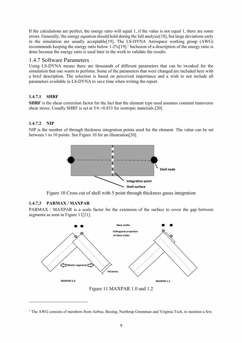
1.4.7.3 PARMAX / MAXPAR PARMAX / MAXPAR is a scale factor for the extension of the surface to cover the gap between segments as seen in Figure 11[21].

Figure 11 MAXPAR 1.0 and 1.2

1 The AWG consists of members from Airbus, Boeing, Northrup Grumman and Virginia Tech, to mention a few.

10

1.4.7.4 Sag Sag is a term used in CATIA to describe how well elements in the mesh align to the CAD surfaces[22]. It is the largest distance from the edge of a finite element to the CAD surface/true geometry[22], see Figure 8.

11

2 RELATED WORK The contents of this chapter are presented to show the status of the work done in the field of which this thesis is written. The presentation of this information should help readers understand the relationship between work done for this thesis and previous work done. Further, this chapter aims to argue for a research gap which the thesis aims to close. If there exist not a research gap, the thesis is not valid. The usefulness and validity of the thesis is therefore based on whether such a research gap exists. Earlier investigations into the stamping process has found that deformations in die, punch, linkage mechanism, and press frame can cause the blank holder load to decrease by up to 40%[23]. Research and development in press deformations have so far studied the deformation of the press bed and its influence on the deformation of the die[24],[25],[26]. The measured deformations have been used to either rework the die virtually or to negate the physical deformations directly by application of for example hydraulic pressure pads. Knut Großmann et al implemented the elastic effects of the forming press and tools, including an elastic blank holder[8], whether the method also could take into account the twisting of the blank holder is somewhat unclear. Deformations in blank holder for a single action press has been shown to give sometimes large effects on the result of the drawing process[27],[28]. The inclusion of full FE for deformation of the tools comes at a very high numerical cost, to solve this problem one can instead use deformable rigid bodies (DRB). When using DRB the deformation of the tool is a linear combination of several pre-calculated deformation modes of the tool, at each increment in the forming simulation the tool deformation is calculated[28]. Depending on the number of modes used, the calculation time can be significantly reduced[29]. Although the calculation costs have been reduced by using DRB, one still have to create the FE model of the tool, a process that sometimes can take several weeks due to CAD file geometry issues[30]. Although the subject of press elasticity at first glance may seem quite well developed, Pilthammar argues that the current methods used are still only on a technology readiness level (TRL) of 3 to 5 on a scale of 1 to 9[1]. Where TRL 1 represents the basic principles being observed and reported, and TLR 9 is a fully working system that is proven successful[31]. Using these observations, one could argue that there is a research gap of about 5 to 6 TRL in today’s SMF simulations of elastic properties of press and die, and about 4 TRL for friction modelling in SMF. According to Pilthammar further research could try and find the best method for building robust, fast and nimble FE models that include elasticity of press lines and stamping dies on an industrial scale. Since the blank holder is a part of the die, which is a part of the press line[2], this thesis could try and create or find such a method.

12

3 METHODS

3.1 Development method 3.1.1 Main method description The main method chosen for this thesis is the simulation method. The arguments for using this method are presented in the method argumentation chapter, subchapter simulation, found below. Simulation is a method used for substantiating claims and answering research questions, see for example Easterbrook[32] and Gilbert and Troitzsch [33], it makes use of a model which is a simplification of the real world[33]. An example would be a rectangular box used for estimating drag compared to using the true physical shape of the car. The steps involved in simulation are displayed in Figure 12 based on Rose et al [34]. It is also possible to view the simulation as an iterative process where one starts with a simple model and verify it, make a new model adding more complexity and verifying that, this process can be repeated until one has reached a satisfactory accuracy[34].

Figure 12 Common steps in simulation methodology

Model design entails gathering some data relevant to the problem and necessary for the construction of the model[33]. It is also a stage where one start to consider how detailed the model should be[33]. A very complex model will increase the amount of verification and validation that is needed later[33]. Model building is the step where the actual model is constructed[33]. One can choose to construct the model almost from scratch using computer languages such as Python, C++[33], Matlab, etc. One can also choose to use specialized software[33]. For Finite Element modeling there are several programs available to choose from, such as ABAQUS, COMSOL, ANSYS and LS-DYNA to mention a few. Model verification is the third step in the simulation methodology where one checks that the model is behaving as expected[33]. Running of simulation is the step where one experiments with the settings and makes it possible to test assumptions made in the construction of the model[34]. Validating the model is the final step, this is where one checks that the model is a good representation of the system that one wishes to model[34]. If the model is too simple compared to the modeled system, the resulting accuracy may not be good enough[34].

13

3.1.2 Secondary methods description and usage

3.1.2.1 Literature review When doing a literature review the literature to include can be identified by use of systematic literature review (SLR) or by the snowballing method. In SLR a set of databases are chosen to sample from. Search strings including terms relevant to the research question are formulated and used in the chosen databases. The resulting articles from the search are then screened by title, keyword and abstract, if they pass the screening process they are called primary sources. The primary sources are then checked if they contain relevant references. Once the collection of sources is concluded they are again screened against a detailed set of inclusion criteria[35]. The method of forward and backward snowballing is described by Wohlin [36] as a method where a set of articles are chosen as start set. Using backward snowballing the reference list of the start set is used for finding other articles to include. Before including articles from the reference list, the articles are examined and excluded based on properties such as language, title, authors and type of publication etc. The final decision of inclusion of a paper is based on the full paper. The reference lists of the papers deemed worthy to be included are then used to find new articles. This process is repeated until no new papers are found[36]. The related work chapter was conducted as an unstructured snow ball sampling. The article named “Characterizing the Elastic Behaviour of a Press Table through Topology Optimization” was chosen as a start article. The choice of starting article was based on its closeness to the topic this author was interested in.

3.1.2.2 Gathering data from the customers Among the first tasks when developing a new product is the identification of customer needs, in the product development process presented by Ulrich and Eppinger this is included in phase 1[4]. They argue that the identification of customer needs is a five-step process. The five steps are gathering data, interpreting data, organizing the data, establishing the relative importance of needs and reflecting on the process[4]. There are three common methods of gathering data; interviews, focus groups and observation of product in use[4]. The data from the customer ( Volvo Cars) was gathered by use of unstructured interviews and discussions with Mats Sigvant at VCBC. The choice of using Mats Sigvant as the person to interview was based on his previous work in the field, position at Volvo Cars and his availability to the author of this thesis due to him being the secondary supervisor.

3.1.3 Method argumentation

3.1.3.1 Simulation The formulation of the research question has in this case locked in the method to use, that is the question is whether changes in how simulation will be performed will give markedly better simulation results. It is therefore hard to argue for other methods that would give insight into the results reported by the simulation. An extensive literary review might have shed light on this but would also have made up the major part of the thesis. However, this thesis wanted just not to prove that the simulations could be improved but establish the process for determining and including the deformations of the blank holder loads into the SMF software. This process could perhaps have been found via extensive literature review but the underlying goals by the author of this thesis was to create his own models and simulations both from a learning perspective but also from the satisfaction derived by creating something by himself. The benefits of using simulations are that once the model is built the tests done are relatively cheap. The downsides are that the model is only as good as the data used to build it. Both the construction of the model and the debugging of it can be very time consuming, which happened to be true for this case.

14

3.1.3.2 Literature review Proper use of the snowballing method was shown by [36] to arrive at the same number of articles or more than two SLRs published by MacDonell et al [37]. Only using backward snowballing was shown by Jalali and Wohlin [38] to give 15 unique papers compared to 26 unique papers when using an SLR. The answer to the research question did not seem to be highly dependent on whether an SLR or a backward snowballing was used[38]. It is possible that the snowballing method could be sped up by the use of citation network analysis, see for example Lecy and Beatty [39] where the data was collected automatically and identified 80% of the key articles in the field using three forward snowballing iterations with a sampling rate of 10% at each level. Since SLRs are time consuming[38], the author of this thesis chose to use snowballing instead of SLR.

3.1.3.3 Gathering data from the customers The focus group method was deemed too expensive to use since they usually cost 5000$ per group. Interviews was viewed as a possible way of gathering data since the writer had access to Dr. Mats Sigvant, the technical expert in sheet metal forming at Volvo Cars in Olofström. Since the writer also had some access to the production facilities as well as the offices, the method of observing the product in use seemed viable as well[4].

3.1.4 Limits and threats to validity of methods

3.1.4.1 Simulation According to [12] it is required that one has a profound understanding of the underlying theories and limitations when using FEM for simulation if one is to get meaningful results. The author acknowledges that he has some knowledge of the theories behind the FEM, but that it is not at the same level as for example the authors of [12] or [13].

3.1.4.2 Literature review The author of [36] had read the SLR published in [37] 6 months prior to replicating them using the snowball method. This prior knowledge may have had a positive impact on the number of articles identified, thereby making the snowball method appear better than it is. The author of this thesis did not use the same strictness and rigor when conducting the snowballing for this thesis which may very well have led to the fact that there are many relevant articles that were not included. There is a possibility that the choice of starting article may also have been biased since many of the authors from the starting article are connected to BTH, the same institute at which this thesis was written.

3.1.4.3 Gathering data from the customers Since only one person was interviewed, although for longer than one hour, it is possible that the percentage of needs identified was not very high as if more people had been interviewed. See for example work done by Griffin and Hauser [40] where a beta binomial model adopted after interviews with 30 people indicated that a one person interview is only likely to produce ca 10% of the needs. It should be noted that the numbers may vary with product categories and interviewing techniques. After the interview has been conduct the transcripts from the interview need to be analyzed to identify customer needs. Of all the needs available in the transcripts one may need as many as seven people analyzing the data to be able to identify 99% of the needs. As this thesis used only one person for data analysis only about 55% of the needs available in the transcripts would have been identified. If only 10% of needs were available in the transcripts from the interview, then by multiplying this with 0.55, the needs identified by this thesis could be as low as 5% of the total available needs.

15

Since the work incorporated Volvo Cars as the sole sheet metal forming corporation in its contacts, it is possible that the needs identified are limited to the specific conditions at the Volvo Cars Body Component facility.

3.1.5 Choice of tools for conducting simulations FEM is used to model the blank holder loads and deformation. The complex shape of the blank holder renders analytical methods less appealing. Instead, the FE method is judged to be more appropriate for this problem. FEM has been successfully used in previous work on for example blank holder deformation in a single action die[27]. Once results from FEM are incorporated into AutoForm, AutoForm was used to do SMF simulations. It was hoped that the inclusion of deformation should give results from AutoForm that were closer to the measured values of spring back. An exploded view of the parts used for the second model is shown below in Figure 13.

Figure 13 Overview of the Second Model

3.2 General LS-DYNA Settings 3.2.1.1 Consistent units In LS-DYNA the S2 system for consistent units were chosen. Length in mm, and Force in Newtons. Values for pressure would therefore be in MPa.

3.2.1.2 Mass scaling Mass scaling was used to reduce simulation time, for the initial model, a value of -1.2E-6s was chosen, about 100 times larger than the timestep otherwise required by the smallest element. By specifying a negative value, mass is only added to elements that have a time step less than; TSSF*abs(DT2MS)[41]. TSSF = Scale factor for the computed time step. DT2MS = time step size for mass scaled solutions. One can also choose to specify a positive value which will add or take away mass from all elements so that their timesteps are the same. The recommendation from LS-DYNA however, is to use negative values. A second run is needed with different mass scaling settings to see how much mass scaling is affecting the results.

16

Alternatively, one can instead use time scaling which means that the load rate is increased, as with mass scaling one needs to verify results by running a second simulation to estimate how sensitive the model is to the increased load rate.

3.3 Model Creation 3.3.1 Meshing

3.3.1.1 Solid tools Some geometrical features of the solids were removed before meshing since they were believed to influence the results minimally and to simplify the meshing process. The solid tools were meshed in CATIA using tetrahedrals. The mesh used a global size of 50mm with a local sag of 10mm, and a refined size on contact surfaces of about 8mm with local sag of 0.1mm. The refinement along the draw beads were done in hopes of getting more accurate contact results.

3.3.1.2 Pins Since previous works on press tools had shown that it was possible for some of the pins to lose contact with the blank holder, the pins were incorporated as separate entities, fixed at their ends and with contact formulation with blank holder. To reduce model complexity the pins were modeled as boxes with adjusted Youngs modulus to give approximately the same stiffness as the original pins, which were approximated as being cylindrical their entire length and with dimensions 250mm long with a 60mm diameter. The meshing alternatives of the pins are shown in Figure 14. To reduce further work the modified pins were meshed with free tetrahedrals instead of swept bricks. Another idea would have been to create single brick elements inside LS-PrePost, but since there were 48 needed in total, and that they also would have to be positioned manually in LS-PrePost, made the labor cost higher than the expected benefits.

Figure 14 Original Pin geometry meshed with 20 to 10 mm elements (left) Modified Pin

(right) not to scale, 48 is the number of pins

3.3.1.3 Sheet Metal The sheet metal was meshed in AutoForm using triangular shells and a maximum of 5 refinement stages resulting in elements with side length ranging from 20mm to about 0.65mm.

3.3.1.4 Die milling surface The tool surface meshes for upper matrix and blank holder were meshed with standard simulation settings in AutoForm. When imported into LS-PrePost it was however revealed that there were about 2600 elements with sides smaller than 1E-20 mm, which had to be removed. At this point it was realized

17

that LS-PrePost V 4.3 did not update the mesh after the elements were removed, and therefore the version was switched to V 4.5. The tool surface meshes were defined as 0.01mm thick and needed to be specified as a Null material in LS-PrePost. Further the tool surface mesh had to be trimmed at the edges since elements extending beyond the solid caused unstable results like the ones in Figure 15 and Figure 16.

Figure 15 Unstable behavior

Figure 16 Unstable behavior

3.3.2 Material properties and element types Using data provided by Volvo Cars the materials were assigned the properties seen in Table 1, except for the pins which uses properties of steel from “Formel och tabellsamling för teknologi och konstruktion” by Karl Björk[42]. For solids, the element type #10 was used, this is a one-point constant stress tetrahedral element. For shells, the element type #2 was used, this is the default element type for shells in LS-DYNA, used for its efficiency. The element type is based on the Mindlins och Reissners plate theory. Table 1 Parts material properties and element types

PARTS YOUNG’S MODULUS

DENSITY POISSON RATIO ELEMENT TYPE

BLANK HOLDER AND UPPER MATRIX

176kN/mm2 7.2kg/dm3 0.275 Solid 10

SHEET METAL 210kN/mm2 7.8kg/dm3 0.3 Shell 2 PINS 9kN/mm2 7.85kg/dm3 0.31 Solid 10

3.3.3 Boundary conditions, contacts and loading The blank holder was restricted for movement in X and Y directions according to Figure 17, due to how it is mounted in the press. The upper matrix was constrained for all rotations and all translations except in Z direction in the nodes highlighted in Figure 18.

18

Figure 17 Boundary Conditions for blank holder, X and Y direction

Figure 18 Upper Matrix with nodes locked in X and Y direction, as well as all rotations

highlighted

Figure 19 Pins with bottom nodes locked for all DOFs

To be able to extract reaction forces on the individual pins, the contact “surface to surface” was used. The same contact type was used between sheet metal and solids. The load of 1800kN was applied as a distributed pressure on top of the upper matrix. The area on which the pressure was applied was measured on the mesh in CATIA.

19

3.3.4 Contact definitions The contact between the tool surface mesh and the solids were defined using “Tied Nodes To Surface Constrained Offset”. This contact ties nodes on the milling surface mesh to the surface of the solid mesh. To overcome the fact that the solid mesh was rougher than the fine mesh, causing gaps in distance to the fine mesh, the SST and MST value was set to -10, thereby making it easier to tie the tool surface shell mesh to the solid mesh. The gaps in distance between solid and fine mesh is shown in Figure 20, where the solid sometimes protrudes through the milling surface mesh and sometimes lies beneath it. The minus sign for SST and MST makes it so that the value is treated as an absolute value.

Figure 20 Light Yellow (Solid) Dark Yellow (blank holder milling surface mesh)

For the contact between tool surface and sheet metal the contact type “Forming one-way surface to surface” was used. Important parameters pertaining to this contact was the PARMAX value which had to be increased from standard value of 1.025 to 1.5 for better contact in draw beads, see Analysis for more info.

3.4 GOM Inspect comparison creation Sheet metal mesh after forming from AutoForm is imported to GOM Inspect, along with the scanned sheet. The comparison was created by the following steps: AutoForm mesh is transformed to same coordinate system as used in LS-DYNA by Manual alignment - Set Matrix in GOM. The AutoForm sheet is set as actual CAD geometry to which the scanned geometry was compared by use of best fit.

20

4 RESULTS

4.1 Reaction forces on pins The reaction forces on the pins were extracted at t=0.08s. The sum of the reaction forces was at that time 1760 kN. Due to what appeared like a linear behavior of the structure the values were then scaled to sum up to a total of 1800kN when later used in AutoForm. To illustrate the force and spatial distribution, a 3D bar plot was created, as seen in Figure 21.

Figure 21 Reaction forces on pins

Another way to illustrate the results are illustrated in Figure 22 along with the numbering used for the individual pins.

Figure 22 Extracted pin reaction forces and pin numbering

An alternative way of calculating the pin reaction forces is with the help of a 6th order Butterworth filter. Set with a cut off frequency of 100Hz, the presumed 1DOF response of the system can be filtered out, as seen in Figure 23. Initially there is no reaction force present since the press tools have yet to make

21

contact. At about t=0.016 the upper matrix bumps into the sheet metal and blank holder which is seen in the sudden spike of reaction force. The upper matrix then bounces back off, and this is repeated until t=0.04, where after the reaction force never goes down to 0 again. Instead, the reaction force is rising, albeit with oscillation. Using the filter we get a more steady rise in reaction force. The same filtration can be applied on all the reaction forces and compared to the initial handpicked values, as seen in Figure 24.

Figure 23 Sum of Reaction forces from all pins (fs = 10kHz)

Figure 24 Handpicked vs filtered values, Pins No 1-24

In Figure 24 the values used for AutoForm simulation are shown compared to what they would have been if we instead had used filter before picking them.

22

4.2 Pressure distribution The pressure distribution over the sheet metal is seen in Figure 25. The upper part of the sheet seems to experience much less pressure overall compared to the bottom part. In the corners there are low-pressure areas as well. As seen in Figure 26 there is high pressure on inner and outer short edge. The bottom part has a pressure that is almost twice that of the corner values. In the middle the pressure is zero since there is no contact between the press tools here.

Figure 25 Pressure distribution on sheet metal

Figure 26 Short edge pressure distribution

4.3 AutoForm Implementation In AutoForm a full simulation of the sheet forming was carried out, results for pressure distribution and sheet surface form were extracted.

4.3.1 AutoForm pressure distribution Using the pin reaction forces that we extracted from LS-DYNA we get the a pressure distribution as seen in Figure 27. Comparing max to min of the highlighted values reveals that there is at most a difference of about 16%. There is no pressure in the middle of the sheet metal because we are only making contact with the blank holder and not using the draw punch to form the metal. The bottom edged exhibits a higher pressure compared to the upper edge. The pressure distribution when using standard simulation, i.e. not using the pin reaction forces extracted from LS-DYNA, are shown in Figure 28. In this simulation the upper edge is the one displaying a higher pressure. The difference between highest and lowest pressure of the ones highlighted are in this simulation only about 8%

23

Figure 27 AutoForm blank holder pressure distribution using LS-DYNA forces

Figure 28 AutoForm blank holder pressure distribution using standard simulation

4.3.2 AutoForm complete sheet forming With the standard simulation the following surface deviations after spring back were measured, as seen in Figure 29. Green color indicates a surface deviation of 0 mm, red and yellow indicate that the simulated sheet is above the experimental sheet, and blue colors indicate that the simulated sheet metal is below the experimental sheet. The results seem acceptable except for along the middle of the lower edge where both simulations predict the sheet to be significantly above its measured position. The same measurements were performed with results using forces extracted from LS-DYNA, which are shown in Figure 30.

24

Figure 29 Allact6 Standard simulation surface deviation to scanned sheet metal

Figure 30 Allact6 Simulation with forces extracted from LS-DYNA, surface deviation to

scanned sheet metal

4.4 Simulation guidelines The contents of this chapter are presented upon the request of Volvo Cars[2]. This chapter includes a numbered list of steps to perform when one wants to run a simulation for extraction of the pin reaction forces.

1. Reduce number of CAD models involved by considering their influence on results 2. Reduce CAD model complexity by removing features perceived to have low influence on results 3. Decide on necessary element types, sizes and mesh 4. Inspect mesh and adjust size or type if necessary 5. Export to LS-PrePost and inspect again if mesh was altered in the export 6. Fix mesh imported from AutoForm by removing very short elements, removing duplicate nodes

and adjusting normals 7. Set part properties, LS-DYNA element types, loads, boundary conditions, time steps etc. 8. Change orientation and position if necessary of meshes 9. Define contacts and inspect them 10. Run simulation using the latest version of solver possible 11. Perform necessary verifications 12. Export and filter reaction forces in foe. Matlab

25

5 ANALYSIS AND DISCUSSION

5.1 Reaction forces on pins Initial investigation reveals that the sum of reaction forces on the pins are steadily rising with increased load using a 9-point average. Since the reaction force on each individual pin were more interesting, a study on how stable the distribution of reaction forces was during the loading of the blank holder were performed. To get an overview of how stable the distribution of the reaction force from the pins were, the pins reaction force divided by the sum of reaction force from all pins were plotted in a box plot, see Figure 31. The values were taken from t=0.06 to t=0.09.

Figure 31 Distribution of total reaction force on single pin (Pins 1-24)

As can be deduced from Figure 31 the unfiltered force distribution for a pin can vary by as much as 20%. The conclusion was that one either must filter the distribution ratio or use the median value when extracting the pin reaction forces.

5.2 Pressure distribution The pressure distribution in the beads were quite spotty and not as smooth as expected, marked by white ellipsoids in Figure 32. Colors other than blue indicate pressure. To improve this, the following parameters were changed:

• Changed shell thickness to 0.01mm on milling surface meshes from 0.1mm. • Changed PARMAX to 1.5 in forming contact from 1.025. • Changed NIP sheet metal to 5 from 3 • Changed SHRF to 0.833 from 1

The results were a significantly better contact pressure distribution in the beads. It is suspected that PARMAX was the main contributor to the improvement since the beads contain small radii which means large angular differences between the element surfaces.2

2 No further investigation to verify this was carried out due to time constraints

26

Figure 32 Initial pressure distribution, beads to sheet metal (Left) Improved pressure

distribution beads to sheet metal (Right)

5.3 Autoform implementation 5.3.1 AutoForm pressure distribution vs LS-DYNA If we compare the pressure distribution in LS-DYNA versus that from AutoForm when using the forces from LS-DYNA, they seem quite similar, see Figure 33 and Figure 34. However, the differences are about half as small in AutoForm compared to LS-DYNA. The pressure distribution in AutoForm is very even on the top and bottom, Figure 34, compared to LS-DYNA where we see a rise at the upper corners and mid bottom section,Figure 33. The biggest impact of implementing the forces from LS-Dyna seems to be a shift in pressure between upper and bottom section of the part, see Figure 34 and Figure 35. For the standard simulation the upper part had higher pressure compared to the lower part, introducing the LS-DYNA forces led to the lower part having higher pressure than the upper section.

27

Figure 33 Pressure Distribution in LS-DYNA

Figure 34 Pressure distribution in AutoForm using extracted LS-DYNA forces

Figure 35 Pressure distribution in AutoForm using standard simulation

5.3.2 AutoForm complete sheet forming The standard simulation vs experimental data is shown in Figure 36 and the AutoForm simulation using forces from L-DYNA compared to experimental data are shown in Figure 37. It is somewhat discouraging that the direct implementation of the pin forces did not have much of an impact on the accuracy of the simulation, but rather it seemed to get to slightly worse in some areas, indicated by ellipsoids in Figure 37.

28

Figure 36 Standard simulation

Figure 37 Using extracted LS-DYNA forces

It is possible that the fact that the test specimen was placed off center in the press and that the blank was past its best before date, leading to material property changes and ultimately bad conformity between simulation and test results. These facts however should only affect the sheet forming results and not the pressure distribution on the blank holder.

5.4 Various items To verify the results given by LS-DYNA, the following was analyzed:

• The general behavior of the model throughout the simulation. • Energy ratio • Mass scaling sensitivity • Frequency response of the system • Rigid behavior of upper part of upper matrix • Load curve shape dependency • Pressure in beads

29

5.4.1 General behavior of model throughout the simulation Animation of all plot states appeared to reveal no nonphysical behavior of the model. No exploding meshes, no parts pass through each other. Also, the sheet metal seemed to form well according to the milling surface meshes. The pressure is lower near the corners, this is either because they are furthest away from the center of the applied force, or it could also be due to the issue with the beads on the short end that interefered slightly with each other, and the milling surface mesh did not fully resolve this issue. To resolve this one could edit the cad models so that they match with each other and see if that solves the issue. Right on the tip of the corners high pressure appears again, the reason for this could be that the surrounding structure of the blank holder that is not being pushed down by the upper matrix is oscillating up and down resulting in stress concentrations in the corners. To resolve this one could possibly have removed this surrounding structure during the meshing phase.

5.4.2 Energy Ratio To check the validity of simulation results the energy data reported by LS-DYNA was used. Initially only the solution with a DT = 0.6E-6s had an energy ratio increase of less than 2% in the timespan of interest.

5.4.3 Sensitivity to mass scaling To see if the results were misleading due to mass scaling effects, different mass scaling settings were used. One used a DTMS of 1.2e-6s and another used 0.6E-6s. 0.6E-6s added 56g, equivalent to 0.9% of total mass. 1.2E-6s added 460g, equivalent to a 7.4% increase in mass.3. Since one goal of the simulation was to get reaction forces from the different pins, the sum of reaction forces in vertical direction were analyzed. Using a 9-point average it was concluded that mass scaling only seemed to affect the solution to a small extent, see Table 2. Table 2 Mass scaling sensitivity

DTMS (S) SUM OF REACTION FORCES ON PINS (MN) @ T=0.08

SIMULATION TIME 112 CORES

MAX ENERGY RATIO INCREASE T=0.02 TO T=0.08S

0.6E-6 1.76 1hr 21 min 1.1% 1.2E-6 1.76 41min 3.0% 2.4E-6 1.75 21min 4.2% 4.8E-6 1.78 11min 2.6%

5.4.4 Frequency response of the system The frequency of the oscillations at around t=0.08 were measured on two periods 1/((0.0857-0.0753)/2) = 190Hz, see Figure 38. It was suspected the system was behaving as a simple 1 DOF system where the mass was the mass of the solid tools and the sheet metal and the spring was the supporting pins. The natural frequency of such a 1 DOF system is calculated below. In a single mass spring system, the natural frequency of the system can be calculated according to[43]:

𝑓𝑛 =1

2𝜋√

𝑘

𝑚

𝑓𝑛 = natural frequency (Hz) k = spring stiffness (N/m)

m = mass (kg) The k value of the pins can be approximated by[42]: 3 Due to TSSFAC default value of 0.9, the timesteps used by the simulation were 10% smaller

30

𝑘 =𝐴𝐸

𝐿

A = cross sectional area of the spring(m2) E= Young´s modulus (Pa) L=length of the spring (m)

The mass of the blank holder and the upper matrix is about 5960kg The calculated k value for the sum of all springs was about 3.8E8 N/m The cross-sectional area of the pins was about 0.3m2 The length of the pins was 0.08m. This resulted in a calculated natural frequency of about 13Hz which is quite far from the measured 190Hz. Therefore, the oscillations must either be originating due to eigen modes or they are artifacts from the system.

Figure 38 Sum of reaction forces over time

5.4.5 Rigid behavior of top of upper matrix Since the top of the upper matrix is attached to the massive slide of the press, it was initially assumed that it could be viewed as being rigid. To reduce modelling time, this boundary condition was first modeled by setting the top nodes of the upper matrix as only having freedom in Z direction and locking them in all other directions as well as locking them rotationally. To evaluate how well this would capture being mounted to a rigid plate, the nodal Z displacement was extracted from the top of the upper matrix in the timespan 0.07 to 0.09s.4 As can be seen in Figure 39, there was a spread of about 60 µm in min/max displacement in Z direction.

4 Model 1.702

31

Figure 39 Nodal displacement upper matrix

5.4.6 Load curve shape dependency To try and reduce contact instabilities, oscillations, and keep the solution more stable, a smoother load curve was implemented. It was created in MATLAB by means of a translated sinusoid which was then scaled to peak at t=0.08s, after t=0.08 the force was kept at maximum to the end of simulation. Plotting the two curves together however reveals that the smoother curve has a steeper slope between t=0.02 and t=0.06, as seen in Figure 40.

Figure 40 Load Curve comparison

Figure 41 Change in energy ratio, Smooth

vs Ramped

The effect of using a smoother load curve was mostly appreciated by looking at the Energy ratio, plotted in Figure 41, which revealed that the smoother curve resulted in a ca 35% reduction in maximum energy ratio increase, and a 28% lower growth ratio, leading to potential longer simulation times while staying below the recommended 2% threshold.5 For the reaction forces however, the smoother curve seems to have a less dramatic effect, other than that time of contact is shifted due to lower initial acceleration. The conclusion was drawn that for this case the simpler ramped load application is fully viable without any significant drawbacks.

5.4.7 Pressure values compared to AutoForm The blank holder pressure extracted from LS-DYNA was two to three times that reported by AutoForm. This raised questions as to what the culprit for this quite significant difference might be.

5 Growth ratio measured by use of ginput on a straight line through middle of measured values from t=0.04 to t=0.09. Max growth ratio difference measured by max value of the curves during the whole simulation time.

32

Since the reaction forces were oscillating to some extent, it was plausible that the interface pressure was extracted at a high point. For example, the force acting on pin 1 is after t=0.08 at min 19.1kN and max 46.7kN, more than twice the difference. However, studying the reaction force from the contact interface showed that the total reaction force from the interface was approximately the same as the applied blank holder pressure. Mesh size influence on pressure distribution was studied by decreasing the largest allowable size of elements on the sheet metal from 20mm to 5mm. The number of refinement steps were reduced so that the smallest element size allowed remained the same. However, this did not influence the results to any greater extent. The next step was to study if the somewhat poor quality of the milling surface meshes were having an influence on the results. Duplicate nodes were merged with a tolerance set to 0.1mm and the normals of the tool surface meshes were adjusted, so that they were facing the sheet metal. This however did not have any effect on the results. Comparing CONTROL_CONTACT settings with the ones used by [44] revealed that they had used OREN = 4 whereas in this project it had been set to 1[44]. Adjusting a non-node merged version did not seem to have any impact on the results. Setting CONTROL_CONTACT = 4 in combination with the adjusted mesh did not have any impact on results.

33

6 CONCLUSION Using LS-DYNA with explicit has some negative drawbacks such as having to deal with oscillations in the solution, and transients states, which made comparisons a bit more difficult. Solution times were kept quite low, some models took about 2h on 28 cores, which could have been further reduced with mass scaling to probably 30min on the same number of cores. Analysis of pressure distribution from LS-DYNA did point to tool deformations as a possible reason for what might be the cause for the difference in draw in between simulation and the scanned sheet metal in some areas. Perhaps the resulting reaction force was not the best method to study sensitivity to mass scaling, maybe one should have used bar plots for reaction forces on half of the pins.

6.1 Reaction forces on pins The reaction forces on the pins for the examined model were quite even. For extraction of the individual forces a filtered solution was a better option. Using LS-DYNA explicit resulted in quite large oscillations in the reaction forces, the source of which have not been identified.

6.2 Pressure distribution The pressure in the beads seemed very sensitive to settings used. Caution is advised when evaluating results in geometrically complex areas.

6.3 Autoform implementation 6.3.1 Autoform pressure distribution vs LS-DYNA Despite our best efforts the pressure values from LS-DYNA never did come close to the values reported by AutoForm. The pressure distribution however, was similar to AutoForm, except for around beads.

6.3.2 Autoform complete sheet forming Direct implementation of the resulting reaction forces on the pins into AutoForm did not improve AutoForm simulation accuracy for the model investigated.

6.4 Research question RQ: Will physically more correct modelling of blank holder load lead to simulations that markedly agree better with available measurements? The answer to the research question is no, the simulation of the sheet metal forming did not markedly agree better with measurements.

34

7 FUTURE WORK For future work one can at least suggest three areas of interest:

• How to transfer contact pressure to AutoForm from LS-DYNA • Adjust LS-DYNA model to closer resemble ideal contact pressure given by AutoForm to get

input on how to configure the physical press. • Work on implementing an implicit solution after an initial explicit.

7.1 Contact pressure transfer to AutoForm Using the same amount and location of physical pins in AutoForm did not result in quite the same pressure distribution as that reported by LS-DYNA. To resolve this, it is possible that using a different number of pins, in different locations, might result in a pressure distribution closer to that reported by LS-DYNA.

7.2 Contact pressure adjustment in LS-Dyna By removing certain pins and/or adding shims to certain pins in LS-Dyna, it is possible that one could manipulate the pressure distribution so that it becomes more evenly distributed and thereby closer to the ideal results reported by AutoForm.

7.3 Implicit analysis implementation One could also compare the benefits of instead running the simulation implicitly in LS-DYNA or a combination thereof. Potential drawbacks would be longer simulations times but having the benefit of lowering post processing analysis.

35

REFERENCES [1] J. Pilthammar, “Elastic Press and Die Deformations in Sheet Metal Forming Simulations,”

Lic. Dissertation, Dept. Mec. Eng. BTH, Karlskrona, Sweden, 2017. [2] “Interview with Mats Sigvant,” 02-Feb-2018. [3] “This is Volvo Cars,” volvocars.com. [Online]. Available:

https://www.volvocars.com/us/about/this-is-volvo-cars. [Accessed: 02-Feb-2019]. [4] K. T. Ulrich and S. D. Eppinger, Product design and development, 5th ed. New York, NY,

USA: McGraw-Hill, 2012. [5] K.-H. Robèrt, Sustainability handbook : planning strategically towards sustainability /

contributors: Karl-Henrik Robèrt [och 13 andra]. Lund: Studentlitteratur, 2012. [6] L. Hågeryd, S. Björklund, M. Lenner, and I. Andersson, Modern produktionsteknik. D. 1.

Stockholm: Liber, 2002. [7] T. Altan and E. Tekkaya, Sheet Metal Forming : Fundamentals. Materials Park: ASM

International, 2012. [8] K. GROßMANN, H. Wiemer, A. Hardtmann, and L. Penter, “The advanced forming

process model including the elastic effects of the forming press and tool,” Archives of Civil and Mechanical Engineering, vol. 8, no. 3, pp. 41–54, Jan. 2008.

[9] “Own observation of strain measurement performed by Sheet metal manufacturer at VCBC Olofström in February 2018.”

[10] “ARGUS,” GOM, 2014. [11] T. Jansson et al., “Optimization of draw-in for an automotive sheet metal part: an

evaluation using surrogate models and response surfaces,” Journal of Materials Processing Technology, vol. 159, no. 3, p. 426, 2005.

[12] N. Saabye Ottosen and H. Petersson, Introduction to the finite element method. New York: Prentice Hall, 1992.

[13] G. Broman, Computational engineering. Karlskrona: Avdelningen för maskinteknik, Blekinge tekniska högskola, 2003.

[14] “Presentation during the course Computational Engineering 1 at BTH.” [15] “LS-DYNA,” lstc.com. [Online]. Available: http://www.lstc.com/products/ls-dyna.

[Accessed: 31-Jan-2019]. [16] “MATLAB MathWorks,” mathworks.com. [Online]. Available:

https://se.mathworks.com/products/matlab.html. [Accessed: 09-Feb-2019]. [17] L. Wei and Y. Yuying, “Multi-objective optimization of sheet metal forming process using

Pareto-based genetic algorithm,” Journal of Materials Processing Technology, vol. 208, no. 1, pp. 499–506, Nov. 2008.

[18] “Energy data,” Welcome to the LS-DYNA support site. [Online]. Available: https://www.dynasupport.com/tutorial/ls-dyna-users-guide/energy-data. [Accessed: 31-Mar-2019].

[19] LS-DYNA Aerospace working group, “Modeling Guidelines Document Version 17-1.” 23-Sep-2017.

[20] LS-Dyna Keyword User’s Manual Volume 1, 10th ed., Livermore Software Technology Corporation, Livermore, CA, USA 2017.

[21] “Contact parameters,” Welcome to the LS-DYNA support site. [Online]. Available: https://www.dynasupport.com/tutorial/contact-modeling-in-ls-dyna/contact-parameters. [Accessed: 31-Mar-2019].

[22] “Creating Octree 3D Mesh Parts.” [Online]. Available: http://catiadoc.free.fr/online/cfyuganalysis_C2/cfyuganalysis3dmeshpart.htm. [Accessed: 31-Mar-2019].

[23] M. E. Dingle, P. D. Hodgson, and M. . Cardew-Hall, “Analysis of the Elastic Behavior of the Press Systems in Draw Die Forming,” presented at the Innovations in processing and

36

manufacturing of sheet materials., 2001. [24] J. Pilthammar, M. Sigvant, M. Hansson, E. Pálsson, and W. Rutgersson, “Characterizing

the Elastic Behaviour of a Press Table through Topology Optimization,” J. Phys.: Conf. Ser., vol. 896, no. 1, p. 012068, 2017.

[25] H.-W. Wagener, “New developments in sheet metal forming: sheet materials, tools and machinery,” Journal of Materials Processing Technology, vol. 72, no. 3, pp. 342–357, Dec. 1997.

[26] R. Struck, S. Kulp, B. –. Behrens, and R. Krimm, Investigation of Impacts on the Required Press Force. .

[27] J. Pilthammar, M. Sigvant, and S. Kao-Walter, “Including die and press deformations in sheet metal forming simulations,” J. Phys.: Conf. Ser., vol. 734, no. 3, p. 032036, 2016.

[28] R. A. Lingbeek, V. T. Meinders, and S. Ohnimus, “Compensation of deep drawing tools for springback and tool-deformation,” presented at the IDDRG 2008, 2008.

[29] J. Blitzenbauer, U. Franz, and K. Schweizerhof, Deformable Rigid Bodies in LS-DYNA with Applications - Merits and Limits. 2005.

[30] E. Palsson and M. Hansson, “Press Measurements and Virtual Rework of Stamping Dies,” M.S. thesis, Dept. Mec. Eng., BTH, Karlskrona, Sweden, 2017.

[31] “TECHNOLOGY READINESS LEVELS A White Paper April 6, 1995 John C. Mankins Advanced Concepts Office Office of Space Access and Tech.” [Online]. Available: http://scholar.googleusercontent.com/scholar?q=cache:uyYF4gORE_oJ:scholar.google.com/&hl=en&as_sdt=0,5. [Accessed: 23-Jan-2018].

[32] S. Easterbrook, “Empirical research methods in requirements engineering,” in 15th IEEE International Requirements Engineering Conference, New Delhi, India, October, 2007, pp. 15–19.

[33] N. Gilbert and K. Troitzsch, Simulation for the Social Scientist. Berkshire: McGraw-Hill Education, 2005.

[34] S. Rose, N. Spinks, and A. I. Canhoto, Management research: Applying the principles. Routledge, 2014.

[35] P. Brereton, B. A. Kitchenham, D. Budgen, M. Turner, and M. Khalil, “Lessons from applying the systematic literature review process within the software engineering domain,” Journal of Systems and Software, vol. 80, no. 4, pp. 571–583, Apr. 2007.

[36] C. Wohlin, “Guidelines for snowballing in systematic literature studies and a replication in software engineering,” in In 8th International Conference on Evaluation and Assessment in Software Engineering (EASE 2014, 2014, pp. 321–330.

[37] S. MacDonell, M. Shepperd, B. Kitchenham, and E. Mendes, “How Reliable Are Systematic Reviews in Empirical Software Engineering?,” IEEE Transactions on Software Engineering, vol. 36, no. 5, pp. 676–687, Sep. 2010.

[38] S. Jalali and C. Wohlin, “Systematic literature studies: database searches vs. backward snowballing,” in Proceedings of the ACM-IEEE international symposium on Empirical software engineering and measurement - ESEM ’12, Lund, Sweden, 2012, p. 29.

[39] J. D. Lecy and K. E. Beatty, “Representative Literature Reviews Using Constrained Snowball Sampling and Citation Network Analysis,” Social Science Research Network, Rochester, NY, SSRN Scholarly Paper ID 1992601, Jan. 2012.

[40] A. Griffin and J. R. Hauser, “The voice of the customer,” Marketing science, vol. 12, no. 1, pp. 1–27, 1993.

[41] “Mass scaling — LS-DYNA Support,” dynasupport.com. [Online]. Available: https://www.dynasupport.com/howtos/general/mass-scaling. [Accessed: 01-Oct-2018].

[42] K. Björk, Formel- och tabellsamling för teknologi och konstruktion M. Märsta: K. Björk, 1992.

[43] A. Brandt, Noise and vibration analysis : signal analysis and experimental procedures.

37

Chichester ; Wiley, 2011. [44] M. Lind and V. Sjöblom, “Industrial Sheet Metal Forming Simulation with Elastic Dies,”

M.S. thesis, Dept. Mec. Eng., BTH, Karlskrona, Sweden, 2018.

Extraction of tool reaction forces using LS- DYNA and its ...

Documents

Transcript of Extraction of tool reaction forces using LS- DYNA and its ...