Extra High Voltage Ac
535
-
Upload
luis-vasquez-restrepo -
Category
Documents
-
view
198 -
download
16
description
Extra High Voltage Ac
Transcript of Extra High Voltage Ac


This pageintentionally left
blank

Copyright © 2006, 1990, 1986, New Age International (P) Ltd., PublishersPublished by New Age International (P) Ltd., Publishers
All rights reserved.
No part of this ebook may be reproduced in any form, by photostat, microfilm,xerography, or any other means, or incorporated into any information retrievalsystem, electronic or mechanical, without the written permission of the publisher.All inquiries should be emailed to [email protected]
PUBLISHING FOR ONE WORLD
NEW AGE INTERNATIONAL (P) LIMITED, PUBLISHERS4835/24, Ansari Road, Daryaganj, New Delhi - 110002Visit us at www.newagepublishers.com
ISBN (13) : 978-81-224-2481-2

To
My Mother and Sister
both brave women who fought and won over their common enemy‘cancer’ in their seventies and sixties to give hope to younger
generation of their sex, this book is lovingly dedicated.

This pageintentionally left
blank

It gives me pleasure to write the foreword to the book 'Extra High Voltage A.C. TransmissionEngineering' authored by Rakosh Das Begamudre, Visiting Professor in Electrical Engineeringat the Indian Institute of Technology, Kanpur. The field of e.h.v. is a very growing and dynamicone on which depends to a large measure the industrial growth of a developing country likeours. A course in this subject is offered for advanced under-graduate and postgraduate students,and the Institute also organized a short-term course for teachers in other learned institutionsand practising engineers in India under the Quality Improvement Programme.
With a background of nearly 35 years in this area in India, Japan, U.S.A. and Canada inteaching, design, research, and development, I consider Dr. Begamudre one of the ablest personsto undertake the task of writing a book, placing his wide experience at the disposal of youngerengineers. He has worked at notable institutions such as the National Research Council ofCanada and the Central Power Research Institute, Bangalore, and several other places. Hispublications in the field of e.h.v. transmission are numerous and varied in extent. The I.I.T.Kanpur offered him Visiting Professorship and I am delighted to introduce the book by him tolearned readers in this important field. It is not only a worthy addition to the technical literaturein this topic but also to the list of text books published in India.
S. SAMPATH
DirectorIndian Institute of Technology
Kanpur
Foreword

This pageintentionally left
blank
Preface to the Third Edition
It is nearly a decade since the publication of the Second Edition of this text-reference bookauthored by me and needs a revision. No significant developments have taken place in thebasic theory and principles of e.h.v. transmission engineering, except for increase intransmission-voltage levels, cables, magnitudes of power-handling capabilities, as well as ofcourse the cost of equipment and lines.
But two problems that need mentioning are: (1) harmonics injected into the system bymodern extensive use and developments in Static VAR systems which have an effect on controland communication systems; and (2) effect on human health due to magnetic fields in thevicinity of the e.h.v. transmission line corridor. The first one of these is a very advanced topicand cannot be included in a first text on e.h.v. transmission engineering, as well as severalother topics of a research nature fit for graduate-level theses and dissertations. The secondtopic is considered important enough from epidemiological point of view to necessitateelaboration. Thus a new addition has been made to Chapter 7 under the title: Magnetic FieldEffects of E.H.V. Lines.
Since the date of publication of the first edition, the I.E.E.E. in New York has thought itfit to introduce an additional transactions called I.E.E.E. Transactions on Power Delivery. Theauthor has expanded the list of references at the end of the text to include titles of significanttechnical papers pertaining to transmission practice.
The author wishes to acknowledge the encouragement received from Sri. V.R. Damodaran,Production Editor, New Age International (P) Ltd., for revising this text-reference book andpreparation of the Third Edition.
Vancouver,
British Columbia, Canada.R.D. BEGAMUDRE

This pageintentionally left
blank
Preface to the First Edition
Extra High Voltage (EHV) A.C. transmission may be considered to have come of age in 1952when the first 380–400 kV line was put into service in Sweden. Since then, industrializedcountries all over the world have adopted this and higher voltage levels. Very soon it was foundthat the impact of such voltage levels on the environment needed careful attention because ofhigh surface voltage gradients on conductors which brought interference problems from powerfrequency to TV frequencies. Thus electrostatic fields in the line vicinity, corona effects, losses,audible noise, carrier interference, radio interference and TVI became recognized as steady-state problems governing the line conductor design, line height, and phase-spacing to keep theinterfering fields within specified limits. The line-charging current is so high that providingsynchronous condensers at load end only was impractical to control voltages at the sending-endand receiving-end buses. Shunt compensating reactors for voltage control at no load and switchedcapacitors at load conditions became necessary. The use of series capacitors to increase power-handling capacity has brought its own problems such as increased current density, temperaturerise of conductors, increased short-circuit current and subsynchronous resonance. All theseare still steady-state problems.
However, the single serious problem encountered with e.h.v. voltage levels is theovervoltages during switching operations, commonly called switching-surge overvoltages. Verysoon it was found that a long airgap was weakest for positive polarity switching-surges. Thecoordination of insulation must now be based on switching impulse levels (SIL) and not onlightning impulse levels only.
From time to time, outdoor research projects have been established to investigate high-voltage effects from e.h.v. and u.h.v. lines to place line designs on a more scientific basis,although all variables in the problem are statistical in nature and require long-term observationsto be carried out. Along with field data, analysis of various problems and calculations using theDigital Computer have advanced the state of the art of e.h.v. line designs to a high level ofscientific attainment. Most basic mechanisms are now placed on a firm footing, although thereis still an endless list of problems that requires satisfactory solution.
During his lecturing career for undergraduate and postgraduate classes in High VoltageA.C. Transmission the author was unable to find a text book suitable for the courses. Theexisting text books are for first courses in High Voltage Engineering concentrating on breakdownphenomena of solid, liquid, gaseous and vacuum insulation, together with high voltage laboratoryand measurement techniques. On the other hand, reference books are very highly specializedwhich deal with results obtained from one of the outdoor projects mentioned earlier. To bridge

the gap, this text-reference book for a course in EHV A.C. Transmission is presented. Thematerial has been tried out on advanced undergraduate and post-graduate courses at the I.I.T.Kanpur, in special short-term courses offered to teachers in Universities and practising engineersthrough the Quality Improvement Programme, and during the course of his lectures offered atother Universities and Institutes. Some of the material is based on the author's own work atreputed research and development organizations such as the National Research Council ofCanada, and similar organizations in India and at Universities and Institutes, over the past 25years. But no one single person or organization can hope to deal with all problems so that overthe years, the author's notes have grown through reference work of technical and scientificjournals which have crystallized into the contents of the book. It is hoped that it will be usefulalso for engineers as well as scientists engaged in research, development, design, and decision-making about e.h.v. a.c. transmission lines.
AcknowledgementsThe preparation of such a work has depended on the influence, cooperation and courtesy
of many organizations and individuals. To start with, I acknowledge the deep influence whichthree of my venerable teachers had on my career—Principal Manoranjan Sengupta at theBanaras Hindu University, Professor Dr. Shigenori Hayashi at the Kyoto University, Japan,and finally to Dean Loyal Vivian Bewley who exercised the greatest impact on me in the HighVoltage field at the Lehigh University, Bethlehem, Pennsylvania, USA. To the Council andDirector of the I.I.T. Kanpur, I am indebted for giving me a Visiting Professorship, to Dr. S.S.Prabhu, the Head of EE Department, for constant help and encouragement at all times. To thecoordinator, Q.I.P. Programme at I.I.T., Dr. A. Ghosh, I owe the courtesy for defraying theexpense for preparation of the manuscript. To the individuals who have done the typing anddrafting, I owe my thanks. My special thanks are due to Mr. H.S. Poplai, Publishing Manager,Wiley Eastern Publishing Company, for his cooperation and tolerence of delays in preparingthe manuscript. Thanks finally are due to my colleagues, both postgraduate students andprofessors, who have helped me at many stages of the work involved in preparing this bookwhile the author was at the I.I.T. Kanpur.
(formerly)Electrical Engineering Department RAKOSH DAS BEGAMUDREIndian Institute of TechnologyKanpur, U.P., 208 016, India.
xii Preface

Contents
Foreword ................................................................................................. viiPreface to the Third Edition .................................................................... ixPreface to the First Edition ...................................................................... xi
Chapter 1 Introduction to EHV AC Transmission .......................................... 1–81.1 Role of EHV AC Transmission ..................................................................11.2 Brief Description of Energy Sources and their Development .....................11.3 Description of Subject Matter of this Book ...............................................4
Chapter 2 Transmission Line Trends and Preliminaries ............................. 9–212.1 Standard Transmission Voltages...............................................................92.2 Average Values of Line Parameters ........................................................ 112.3 Power-Handling Capacity and Line Loss ................................................. 112.4 Examples of Giant Power Pools and Number of Lines ............................ 142.5 Costs of Transmission Lines and Equipment .......................................... 152.6 Mechanical Considerations in Line Performance .................................... 17
Chapter 3 Calculation of Line and Ground Parameters .............................22–603.1 Resistance of Conductors ........................................................................ 223.2 Temperature Rise of Conductors and Current-Carrying Capacity ............ 263.3 Properties of Bundled Conductors ........................................................... 283.4 Inductance of EHV Line Configurations .................................................. 303.5 Line Capacitance Calculation .................................................................. 383.6 Sequence Inductances and Capacitances ................................................. 413.7 Line Parameters for Modes of Propagation ............................................. 443.8 Resistance and Inductance of Ground Return ......................................... 50
Chapter 4 Voltage Gradients of Conductors ............................................... 61–1124.1 Electrostatics .......................................................................................... 614.2 Field of Sphere Gap ................................................................................ 63

xiv Contents
4.3 Field of Line Charges and Their Properties ............................................ 684.4 Charge-Potential Relations for Multi-Conductor lines ............................. 724.5 Surface Voltage Gradient on Conductors ................................................. 764.6 Examples of Conductors and Maximum Gradients on Actual Lines ......... 874.7 Gradient Factors and Their Use ............................................................. 874.8 Distribution of Voltage Gradient on Sub-conductors of Bundle ................ 894.9 Design of Cylindrical Cages for Corona Experiments .............................. 92
Appendix: Voltage Gradients on Conductors in the Presence of GroundWires on Towers .................................................................................. 107
Chapter 5 Corona Effects—I : Power Loss and Audible Noise ................ 113–1375.1 I2R Loss and Corona Loss ..................................................................... 1135.2 Corona-Loss Formulae ......................................................................... 1145.3 Charge-Voltage (q–V) Diagram and Corona Loss ................................... 1185.4 Attenuation of Travelling Waves Due to Corona Loss ........................... 1225.5 Audible Noise: Generation and Characteristics ..................................... 1255.6 Limits for Audible Noise ....................................................................... 1265.7 AN Measurement and Meters ............................................................... 1275.8 Formulae for Audible Noise and Use in Design .................................... 1315.9 Relation Between Single-Phase and 3-Phase AN Levels ........................ 134
5.10 Day-Night Equivalent Noise Level........................................................ 1355.11 Some Examples of AN Levels from EHV Lines ..................................... 136
Chapter 6 Corona Effects—II : Radio Interference .................................. 138–1716.1 Corona Pulses: Their Generation and Properties.................................. 1386.2 Properties of Pulse Trains and Filter Response .................................... 1426.3 Limits for Radio Interference Fields ..................................................... 1446.4 Frequency Spectrum of the RI Field of Line ......................................... 1476.5 Lateral Profile of RI and Modes of Propagation ..................................... 1476.6 The CIGRE Formula ............................................................................. 1516.7 The RI Excitation Function .................................................................. 1566.8 Measurement of RI, RIV, and Excitation Function ................................ 1626.9 Measurement of Excitation Function .................................................... 164
6.10 Design of Filter .................................................................................... 1666.11 Television Interference ......................................................................... 167
Chapter 7 Electrostatic and Magnetic Fields of EHV Lines .................... 172–2057.1 Electric Shock and Threshold Currents ................................................ 1727.2 Capacitance of Long Object ................................................................... 1737.3 Calculation of Electrostatic Field of AC Lines ....................................... 1747.4 Effect of High E.S. Field on Humans, Animals, and Plants ................... 183
Contents xv
7.5 Meters and Measurement of Electrostatic Fields .................................. 1857.6 Electrostatic Induction in Unenergized Circuit of a D/C Line ................ 1867.7 Induced Voltage in Insulated Ground Wires.......................................... 1897.8 Magnetic Field Effects .......................................................................... 1907.9 Magnetic Field of 3-Phase Lines ........................................................... 191
7.10 Magnetic Field of a 6-Phase Line .......................................................... 1997.11 Effect of Power-Frequency Magnetic Fields on Human Health ............. 200
Chapter 8 Theory of Travelling Waves and Standing Waves .................. 206–2358.1 Travelling Waves and Standing Waves at Power Frequency ................. 2068.2 Differential Equations and Solutions for General Case .......................... 2098.3 Standing Waves and Natural Frequencies ............................................ 2158.4 Open-Ended Line: Double-Exponential Response .................................. 2198.5 Open-Ended Line: Response to Sinusoidal Excitation ............................ 2208.6 Line Energization with Trapped-Charge Voltage ................................... 2218.7 Corona Loss and Effective Shunt Conductance ..................................... 2238.8 The Method of Fourier Transforms ...................................................... 2248.9 Reflection and Refraction of Travelling Waves ...................................... 227
8.10 Transient Response of Systems with Series and Shunt LumpedParameters and Distributed Lines ........................................................ 230
8.11 Principles of Travelling-Wave Protection of E.H.V. Lines ..................... 232
Chapter 9 Lightning and Lightning Protection ....................................... 236–2589.1 Lightning Strokes to Lines ................................................................... 2369.2 Lightning-Stroke Mechanism ............................................................... 2379.3 General Principles of the Lightning-Protection Problem ....................... 2409.4 Tower-Footing Resistance ..................................................................... 2439.5 Insulator Flashover and Withstand Voltage .......................................... 2459.6 Probability of Occurrence of Lightning-Stroke Currents ....................... 2459.7 Lightning Arresters and Protective Characteristics .............................. 2469.8 Dynamic Voltage Rise and Arrester Rating ........................................... 2509.9 Operating Characteristics of Lightning Arresters ................................. 251
9.10 Insulation Coordination Based on Lightning ......................................... 254
Chapter 10 Overvoltages in EHV Systems Caused by SwitchingOperations .................................................................................. 259–294
10.1 Origin of Overvoltages and Their Types................................................ 25910.2 Short-Circuit Current and the Circuit Breaker ..................................... 26010.3 Recovery Voltage and the Circuit Breaker ............................................ 26210.4 Overvoltages Caused by Interruption of Low Inductive Current ........... 26410.5 Interruption of Capacitive Currents ...................................................... 265
xvi Contents
10.6 Ferro-Resonance Overvoltages ............................................................. 26610.7 Calculation of Switching Surges—Single Phase Equivalents ................. 26710.8 Distributed-Parameter Line Energized by Source ................................. 27310.9 Generalized Equations for Single-Phase Representation ....................... 276
10.10 Generalized Equations for Three-Phase Systems .................................. 28010.11 Inverse Fourier Transform for the General Case .................................. 28510.12 Reduction of Switching Surges on EHV Systems ................................... 28710.13 Experimental and Calculated Results of Switching-Surge Studies ......... 289
Chapter 11 Insulation Characteristics of Long Air Gaps ......................... 295–31711.1 Types of Electrode Geometries Used in EHV Systems .......................... 29511.2 Breakdown Characteristics of Long Air Gaps ........................................ 29611.3 Breakdown Mechanisms of Short and Long Air Gaps ............................ 29911.4 Breakdown Models of Long Gaps with Non-uniform Fields ................... 30211.5 Positive Switching-Surge Flashover—Saturation Problem .................... 30511.6 CFO and Withstand Voltages of Long Air Gaps—Statistical Procedure . 30811.7 CFO Voltage of Long Air Gaps—Paris's Theory .................................... 314
Chapter 12 Power-Frequency Voltage Control and Overvoltages ............ 318–35812.1 Problems at Power Frequency .............................................................. 31812.2 Generalized Constants .......................................................................... 31812.3 No-Load Voltage Conditions and Charging Current .............................. 32112.4 The Power Circle Diagram and Its Use ................................................. 32312.5 Voltage Control Using Synchronous Condensers .................................. 32812.6 Cascade Connection of Components—Shunt and Series Compensation . 33012.7 Sub-Synchronous Resonance in Series-Capacitor Compensated Lines ... 33712.8 Static Reactive Compensating Systems (Static VAR) ............................. 34512.9 High Phase Order Transmission ........................................................... 355
Chapter 13 EHV Testing and Laboratory Equipment ................................ 359–40813.1 Standard Specifications ......................................................................... 35913.2 Standard Waveshapes for Testing ......................................................... 36113.3 Properties of Double-Exponential Waveshapes ..................................... 36313.4 Procedures for Calculating E,,βα ........................................................ 366
13.5 Waveshaping Circuits: Principles and Theory ....................................... 36813.6 Impulse Generators with Inductance .................................................... 37313.7 Generation of Switching Surges for Transformer Testing ..................... 37613.8 Impulse Voltage Generators: Practical Circuits .................................... 37813.9 Energy of Impulse Generators .............................................................. 381
13.10 Generation of Impulse Currents ........................................................... 385

Contents xvii
13.11 Generation of High Alternating Test Voltage ........................................ 38913.12 Generation of High Direct Voltages ...................................................... 39313.13 Measurement of High Voltages............................................................. 39413.14 General Layout of EHV Laboratories.................................................... 405
Chapter 14 Design of EHV Lines Based upon Steady-State Limits andTransient Overvoltages ............................................................. 409–428
14.1 Introduction ......................................................................................... 40914.2 Design Factors Under Steady State ...................................................... 41014.3 Design Examples: Steady-State Limits .................................................. 41314.4 Design Example—I ............................................................................... 41414.5 Design Example—II .............................................................................. 41914.6 Design Example—III ............................................................................. 42014.7 Design Example—IV ............................................................................. 42114.8 Line Insulation Design Based Upon Transient Overvoltages ................ 423
Chapter 15 Extra High Voltage Cable Transmission ................................. 429–48115.1 Introduction ......................................................................................... 42915.2 Electrical Characteristics of EHV Cables .............................................. 43515.3 Properties of Cable-Insulation Materials ............................................... 44515.4 Breakdown and Withstand Electrical Stresses in Solid
Insulation—Statistical Procedure ......................................................... 45315.5 Design Basis of Cable Insulation ........................................................... 46115.6 Further Examples of Cable Designs ...................................................... 46615.7 Tests on Cable Characteristics .............................................................. 47015.8 Surge Performance of Cable Systems ................................................... 47315.9 Gas Insulated EHV Lines...................................................................... 478
Bibliography ...................................................................................... 482Answers to Problems ........................................................................ 499Index ................................................................................................... 505

This pageintentionally left
blank
1.1 ROLE OF EHV AC TRANSMISSIONIndustrial-minded countries of the world require a vast amount of energy of which electricalenergy forms a major fraction. There are other types of energy such as oil for transportationand industry, natural gas for domestic and industrial consumption, which form a considerableproportion of the total energy consumption. Thus, electrical energy does not represent theonly form in which energy is consumed but an important part nevertheless. It is only 150 yearssince the invention of the dynamo by Faraday and 120 years since the installation of the firstcentral station by Edison using dc. But the world has already consumed major portion of itsnatural resources in this short period and is looking for sources of energy other than hydro andthermal to cater for the rapid rate of consumption which is outpacing the discovery of newresources. This will not slow down with time and therefore there exists a need to reduce therate of annual increase in energy consumption by any intelligent society if resources have to bepreserved for posterity. After the end of the Second World War, countries all over the worldhave become independent and are showing a tremendous rate of industrial development, mostlyon the lines of North-American and European countries, the U.S.S.R. and Japan. Therefore,the need for energy is very urgent in these developing countries, and national policies andtheir relation to other countries are sometimes based on energy requirements, chiefly nuclear.Hydro-electric and coal or oil-fired stations are located very far from load centres for variousreasons which requires the transmission of the generated electric power over very long distances.This requires very high voltages for transmission. The very rapid strides taken by developmentof dc transmission since 1950 is playing a major role in extra-long-distance transmission,complementing or supplementing e.h.v. ac transmission. They have their roles to play and acountry must make intelligent assessment of both in order to decide which is best suited forthe country's economy. This book concerns itself with problems of e.h.v. ac transmission only.
1.2 BRIEF DESCRIPTION OF ENERGY SOURCES AND THEIRDEVELOPMENT
Any engineer interested in electrical power transmission must concern himself or herself withenergy problems. Electrical energy sources for industrial and domestic use can be divided intotwo broad categories: (1) Transportable; and (2) Locally Usable.
1Introduction to EHV AC Transmission

2 Extra High Voltage AC Transmission Engineering
Transportable type is obviously hydro-electric and conventional thermal power. But locallygenerated and usable power is by far more numerous and exotic. Several countries, includingIndia, have adopted national policies to investigate and develop them, earmarking vast sums ofmoney in their multi-year plans to accelerate the rate of development. These are also called'Alternative Sources of Power'. Twelve such sources of electric power are listed here, but thereare others also which the reader will do well to research.
Locally Usable Power(1) Conventional thermal power in urban load centres;(2) Micro-hydel power stations;
(3) Nuclear Thermal: Fission and Fusion;
(4) Wind Energy;(5) Ocean Energy: (a) Tidal Power, (b) Wave Power, and (c) Ocean thermal gradient
power;(6) Solar thermal;
(7) Solar cells, or photo-voltaic power;
(8) Geo-thermal;(9) Magneto hydro-dynamic or fluid dynamic;
(10) Coal gasification and liquefaction;(11) Hydrogen power; and last but not least,
(12) Biomass Energy: (a) Forests; (b) Vegetation; and (c) Animal refuse.
To these can also be added bacterial energy sources where bacteria are cultured todecompose forests and vegetation to evolve methane gas. The water hyacinth is a very richsource of this gas and grows wildly in waterlogged ponds and lakes in India. A brief descriptionof these energy sources and their limitation as far as India is concerned is given below, withsome geographical points.
1. Hydro-Electric Power: The known potential in India is 50,000 MW (50 GW) with 10 GW inNepal and Bhutan and the rest within the borders of India. Of this potential, almost 30% or 12GW lies in the north-eastern part in the Brahmaputra Valley which has not been tapped. Whenthis power is developed it will necessitate transmission lines of 1000 to 1500 kilometres inlength so that the obvious choice is extra high voltage, ac or dc. The hydel power in India canbe categorized as (a) high-head (26% of total potential), (b) medium-head (47%), (c) low-head(7%, less then 30 metres head), and (d) run-of-the-river (20%). Thus, micro-hydel plants andrun-of-the-river plants (using may be bulb turbines) have a great future for remote loads inhilly tracts.
2. Coal: The five broad categories of coal available in India are Peat (4500 BTU/LB*), Lignite(6500), Sub-Bituminous (7000-12000), Bituminous (14,000), and Anthracite (15,500 BTU/LB).Only non-coking coal of the sub-bituminous type is available for electric power productionwhose deposit is estimated at 50 giga tonnes in the Central Indian coal fields, With 50% of thisallocated for thermal stations, it is estimated that the life of coal deposits will be 140 years if
*1000 BTU/LB–555.5 k-cal/kg.

Introduction to EHV AC Transmission 3
the rate of annual increase in installed capacity is 5%. Thus, the country cannot rely on thissource of power to be perennial. Nuclear thermal power must be developed rapidly to replaceconventional thermal power.
3. Oil and Natural Gas: At present, all oil is used for transportation and none is available forelectric power generation. Natural gas deposits are very meager at the oil fields in the North-Eastern region and only a few gas-turbine stations are installed to provide the electric powerfor the oil operations.
4. Coal Liquefaction and Gasification: Indian coal contains 45% ash and the efficiency of aconventional thermal station rarely exceeds 25% to 30%. Also transportation of coal from minesto urban load centres is impossible because of the 45% ash, pilferage of coal at stations wherecoal-hauling trains stop, and more importantly the lack of availability of railway wagons forcoal transportation. These are needed for food transportation only. Therefore, the nationalpolicy is to generate electric power in super thermal stations of 2100 MW capacity located atthe mine mouths and transmit the power by e.h.v. transmission lines. If coal is liquified andpumped to load centres, power up to 7 times its weight in coal can be generated in high efficiencyinternal cumbustion engines.
5. Nuclear Energy: The recent advances made in Liquid Metal Fast Breeder Reactors (LMFBR)are helping many developing countries, including India, to install large nuclear thermal plants.Although India has very limited Uranium deposits, it does possess nearly 50% of the world'sThorium deposits. The use of this material for LMFBR is still in infant stages and is beingdeveloped rapidly.
6. Wind Energy: It is estimated that 20% of India's power requirement can be met withdevelopment of wind energy. There are areas in the Deccan Plateau in South-Central Indiawhere winds of 30 km/hour blow nearly constantly. Wind power is intermittent and storagefacilities are required which can take the form of storage batteries or compressed air. For anelectrical engineer, the challenge lies in devising control circuitry to generate a constantmagnitude constant-frequency voltage from the variable-speed generator and to make thegenerator operate in synchronism with an existing grid system.
7. Solar-Cell Energy: Photo-voltaic power is very expensive, being nearly the same as nuclearpower costing U.S.$ 1000/kW of peak power. (At the time of writing, 1 U.S$ = Rs. 35). Solarcells are being manufactured to some extent in India, but the U.S.A. is the largest supplierstill. Indian insolation level is 600 calories/ sq. cm/day on the average which will generate 1.5kW, and solar energy is renewable as compared to some other sources of energy.
8. Magneto Hydro-Dynamic: The largest MHD generator successfully completed in the worldis a 500 kW unit of AVCO in the U.S.A. Thus, this type of generation of electric energy has verylocal applications.
9. Fuel-Cell Energy: The fuel-cell uses H-O interaction through a Phosphoric Acid catalyzer toyield a flow of electrons in a load connected externally. The most recent installation is by theConsolidated Edison Co. of New York which uses a module operating at 190°C. Each cell develops0.7 V and there are sufficient modules in series to yield an output voltage of 13.8 kV, the sameas a conventional central-station generator. The power output is expected to reach 1 MW.
10. Ocean Energy: Energy from the vast oceans of the earth can be developed in 3 differentways: (i) Tidal; (ii) Wave; and (iii) Thermal Gradient.

4 Extra High Voltage AC Transmission Engineering
(i) Tidal Power: The highest tides in the world occur at 40 to 50° latitudes with tides upto 12 m existing twice daily. Therefore, Indian tides are low being about 3.5 m in theWestern Coast and Eastern rivers in estuaries. France has successfully operated a240 MW station at the Rance-River estuary using bulb turbines. Several installationsin the world have followed suit. The development of Indian tidal power at the GujaratCoast in the West is very ambitious and is taking shape very well. Like wind power,tidal power is intermittent in nature.
The seawater during high tides is allowed to run in the same or different passagethrough the turbine-generators to fill a reservoir whose retaining walls may be up to30 km long. At low-tide periods, the stored water flows back to the sea through theturbines and power is generated.
(ii) Wave Energy: An average power of 25 to 75 kW can be developed per metre of wavelength depending on the wave height. The scheme uses air turbines coupled togenerators located in chambers open to the sea at the bottom and closed at the top.There may be as many as 200-300 such chambers connected together at the topthrough pipes. A wave crest underneath some chambers will compress the air whichwill flow into other chambers underneath which the wave-trough is passing resultingin lower pressure. This runs the air turbines and generates power. Others are Salter'sDucks and Cockerrel's 3-part ship.
(iii) Ocean Thermal Power: This scheme utilizes the natural temperature differencebetween the warm surface water (20°-25°C) and the cooler oceanbed water at 5°C.The turbine uses NH3 as the working fluid in one type of installation which is vaporizedin a heat-exchanger by the warm water. The condenser uses the cooler ocean-bedwater and the cycle is complete as in a conventional power station. The cost of suchan installation is nearly the same as a nuclear power station.
This brief description of 'alternative' sources of electric power should provide the readerwith an interest to delve deeper into modern energy sources and their development.
1.3 DESCRIPTION OF SUBJECT MATTER OF THIS BOOKExtra High Voltage (EHV) ac transmission can be assumed to have seen its development sincethe end of the Second World War, with the installation of 345 kV in North America and 400 kVin Europe. The distance between generating stations and load centres as well as the amount ofpower to be handled increased to such an extent that 220 kV was inadequate to handle theproblem. In these nearly 50 years, the highest commercial voltage has increased to 1150 kV(1200 kV maximum) and research is under way at 1500 kV by the AEP-ASEA group. In India,the highest voltage used is 400 kV ac, but will be increased after 1990 to higher levels. Theproblems posed in using such high voltages are different from those encountered at lowervoltages. These are:
(a) Increased Current Density because of increase in line loading by using series capacitors.
(b) Use of bundled conductors.(c) High surface voltage gradient on conductors.
(d) Corona problems: Audible Noise, Radio Interference, Corona Energy Loss, CarrierInterference, and TV Interference.

Introduction to EHV AC Transmission 5
(e) High electrostatic field under the line.
(f) Switching Surge Overvoltages which cause more havoc to air-gap insulation thanlightning or power frequency voltages.
(g) Increased Short-Circuit currents and possibility of ferro resonance conditions.
(h) Use of gapless metal-oxide arresters replacing the conventional gap-type Silicon Carbidearresters, for both lightning and switching-surge duty.
(i) Shunt reactor compensation and use of series capcitors, resulting in possible sub-synchronous resonance conditions and high shortcircuit currents.
(j) Insulation coordination based upon switching impulse levels.
(k) Single-pole reclosing to improve stability, but causing problems with arcing.
The subject is so vast that no one single book can hope to handle with a description,analysis, and discussion of all topics. The book has been limited to the transmission line onlyand has not dealt with transient and dynamic stability, load flow, and circuit breaking.Overvoltages and characteristics of long airgaps to withstand them have been discussed atlength which can be classified as transient problems. Items (a) to (e) are steady-state problemsand a line must be designed to stay within specified limits for interference problems, coronaloss, electrostatic field, and voltages at the sending end and receiving end buses through properreactive-power compensation.
Chapter 2 is devoted to an introduction to the e.h.v. problem, such as choice of voltage fortransmission, line losses and power-handling capacity for a given line length between sourceand load and bulk power required to be transmitted. The problem of vibration of bundledconductors is touched upon since this is the main mechanical problem in e.h.v lines. Chapters3 and 4 are basic to the remaining parts of the book and deal with calculation of line resistance,inductance, capacitance, and ground-return parameters, modes of propagation, electrostaticsto understand charge distribution and the resulting surface voltage gradients. All these aredirected towards an N-conductor bundle. Corona loss and Audible Noise from e.h.v. lines areconsequences of high surface voltage gradient on conductors. This is dealt fully in Chapter 5. Inseveral cases of line design, the audible noise has become a controlling factor with its attendantpollution of the environment of the line causing psycho-acoustics problems. The material oninterference is continued in Chapter 6 where Radio Interference is discussed. Since this problemhas occupied researchers for longer than AN, the available literature on RI investigation ismore detailed than AN and a separate chapter is devoted to it. Commencing with corona pulses,their frequency spectrum, and the lateral profile of RI from lines, the reader is led into themodern concept of 'Excitation Function' and its utility in pre-determining the RI level of a lineyet to be designed. For lines up to 750 kV, the C.I.G.R.E. formula applies. Its use in design isalso discussed, and a relation between the excitation function and RI level calculated by theC.I.G.R.E. formula is given.
Chapter 7 relates to power frequency electrostatic field near an e.h.v. line which causesharmful effects to human beings, animals, vehicles, plant life, etc. The limits which a designerhas to bear in mind in evolving a line design are discussed. Also a new addition has been madein this chapter under the title Magnetic Field Effects of E.H.V. Lines. Chapters 8-11 are devoted
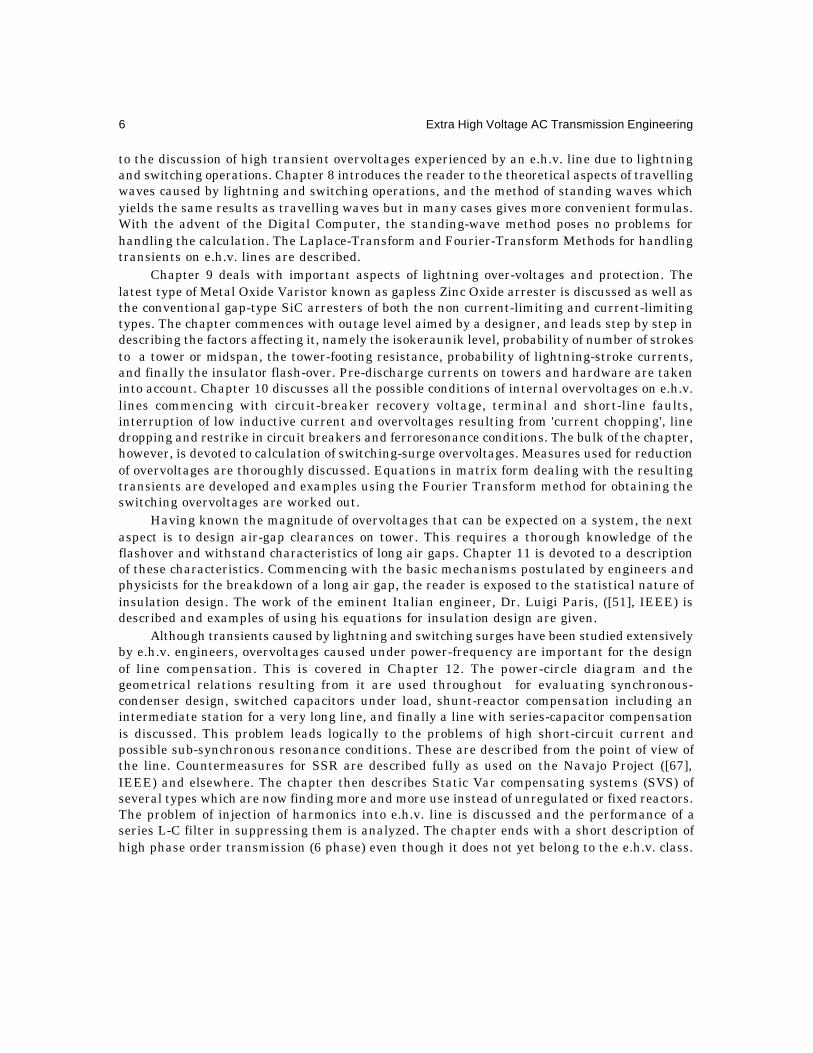
6 Extra High Voltage AC Transmission Engineering
to the discussion of high transient overvoltages experienced by an e.h.v. line due to lightningand switching operations. Chapter 8 introduces the reader to the theoretical aspects of travellingwaves caused by lightning and switching operations, and the method of standing waves whichyields the same results as travelling waves but in many cases gives more convenient formulas.With the advent of the Digital Computer, the standing-wave method poses no problems forhandling the calculation. The Laplace-Transform and Fourier-Transform Methods for handlingtransients on e.h.v. lines are described.
Chapter 9 deals with important aspects of lightning over-voltages and protection. Thelatest type of Metal Oxide Varistor known as gapless Zinc Oxide arrester is discussed as well asthe conventional gap-type SiC arresters of both the non current-limiting and current-limitingtypes. The chapter commences with outage level aimed by a designer, and leads step by step indescribing the factors affecting it, namely the isokeraunik level, probability of number of strokesto a tower or midspan, the tower-footing resistance, probability of lightning-stroke currents,and finally the insulator flash-over. Pre-discharge currents on towers and hardware are takeninto account. Chapter 10 discusses all the possible conditions of internal overvoltages on e.h.v.lines commencing with circuit-breaker recovery voltage, terminal and short-line faults,interruption of low inductive current and overvoltages resulting from 'current chopping', linedropping and restrike in circuit breakers and ferroresonance conditions. The bulk of the chapter,however, is devoted to calculation of switching-surge overvoltages. Measures used for reductionof overvoltages are thoroughly discussed. Equations in matrix form dealing with the resultingtransients are developed and examples using the Fourier Transform method for obtaining theswitching overvoltages are worked out.
Having known the magnitude of overvoltages that can be expected on a system, the nextaspect is to design air-gap clearances on tower. This requires a thorough knowledge of theflashover and withstand characteristics of long air gaps. Chapter 11 is devoted to a descriptionof these characteristics. Commencing with the basic mechanisms postulated by engineers andphysicists for the breakdown of a long air gap, the reader is exposed to the statistical nature ofinsulation design. The work of the eminent Italian engineer, Dr. Luigi Paris, ([51], IEEE) isdescribed and examples of using his equations for insulation design are given.
Although transients caused by lightning and switching surges have been studied extensivelyby e.h.v. engineers, overvoltages caused under power-frequency are important for the designof line compensation. This is covered in Chapter 12. The power-circle diagram and thegeometrical relations resulting from it are used throughout for evaluating synchronous-condenser design, switched capacitors under load, shunt-reactor compensation including anintermediate station for a very long line, and finally a line with series-capacitor compensationis discussed. This problem leads logically to the problems of high short-circuit current andpossible sub-synchronous resonance conditions. These are described from the point of view ofthe line. Countermeasures for SSR are described fully as used on the Navajo Project ([67],IEEE) and elsewhere. The chapter then describes Static Var compensating systems (SVS) ofseveral types which are now finding more and more use instead of unregulated or fixed reactors.The problem of injection of harmonics into e.h.v. line is discussed and the performance of aseries L-C filter in suppressing them is analyzed. The chapter ends with a short description ofhigh phase order transmission (6 phase) even though it does not yet belong to the e.h.v. class.

Introduction to EHV AC Transmission 7
Chapter 13 deals with e.h.v. laboratories, equipment and testing. The design of impulsegenerators for lightning and switching impulses is fully worked out and waveshaping circuitsare discussed. The effect of inductance in generator, h.v. lead, and the voltage divider areanalyzed. Cascade-connected power-frequency transformers and the Greinacher chain forgeneration of high dc voltage are described. Measuring equipment such as the voltage divider,oscilloscope, peak volt-meter, and digital recording devices are covered and the use of fibreoptics in large e.h.v. switchyards and laboratory measurements is discussed.
Chapter 14 uses the material of previous chapters to evolve methods for design of e.h.v.lines. Several examples are given from which the reader will be able to effect his or her owndesign of e.h.v. transmission lines in so far as steadystate and transient overvoltages areconcerned.
The last chapter, Chapter 15, deals with the important topic of e.h.v cable transmission.Cables are being manufactured and developed for voltages upto 1200 kV to match the equipmentand overhead-line voltages in order to interconnect switchyard equipment such as overheadlines to transformers and circuit breakers. They are also used for leading bulk power fromreceiving stations into the heart of metropolitan industrial and domestic distribution stations.In underground power stations, large stations located at dam sites, for under-river and under-sea applications, along railways, over long-span bridges, and at many situations, e.h.v. cablesare extensively used. The four types of e.h.v. cables, namely, high-pressure oil-filled (HPOF)with Kraft paper insulation, the same with composite laminated plastic film and paper insulation(PPLP), cross-linked polyethylene (XLPE), and gas-insulated (SF6) lines (GIL's) or bus ductsare described and discussed. Design practices based on a Weibull Probability Distribution forinitial breakdown voltage and stress and the Kreuger Volt-Time characteristics are also dealtwith. Extensive examples of 132 kV to 1200 KV cables already manufactured or underdevelopment are given.
Each chapter is provided with a large number of worked examples to illustrate all ideas ina step by step manner. The author feels that this will help to emphasize every formula or ideawhen the going is hot, and not give all theory in one place and provide examples at the end ofeach chapter. It is expected that the reader will work through these to be better able to applythe equations.
No references are provided at the end of each chapter since there are cases where onework can cover many aspects discussed in several chapters. Therefore, a consolidated bibliographyis appended at the end after Chapter 15 which will help the reader who has access to a finelibrary or can get copies made from proper sources.
Review Questions and Problems
1. Give ten levels of transmission voltages that are used in the world.
2. Write an essay giving your ideas whether industrial progress is really a measure ofhuman progress.
3. What is a micro-hydel station?
4. How can electric power be generated from run-of-the-river plants? Is this possible orimpossible?

8 Extra High Voltage AC Transmission Engineering
5. What is the fuel used in (a) Thermal reactors, and (b) LMFBR? Why is it calledLMFBR? What is the liquid metal used? Is there a moderator in LMFBR? Why is itcalled a Breeder Reactor? Why is it termed Fast?
6. Draw sketches of a wind turbine with (a) horizontal axis, and (b) vertical axis. Howcan the efficiency of a conventional wind turbine be increased?
7. Give a schematic sketch of a tidal power development. Why is it called a 'bulb turbine'?
8. Give a schematic sketch of an ocean thermal gradient project showing a heat exchanger,turbine-generator, and condenser.
9. List at least ten important problems encountered in e.h.v. transmission which mayor may not be important at voltages of 220 kV and lower.

2.1 STANDARD TRANSMISSION VOLTAGESVoltages adopted for transmission of bulk power have to conform to standard specificationsformulated in all countries and internationally. They are necessary in view of import, export,and domestic manufacture and use. The following voltage levels are recognized in India as perIS-2026 for line-to-line voltages of 132 kV and higher.
Nominal SystemVoltage kV 132 220 275 345 400 500 750
Maximum OperatingVoltage, kV 145 245 300 362 420 525 765
There exist two further voltage classes which have found use in the world but have notbeen accepted as standard. They are: 1000 kV (1050 kV maximum) and 1150 kV (1200 kVmaximum). The maximum operating voltages specified above should in no case be exceeded inany part of the system, since insulation levels of all equipment are based upon them. It istherefore the primary responsibility of a design engineer to provide sufficient and proper typeof reactive power at suitable places in the system. For voltage rises, inductive compensationand for voltage drops, capacitive compensation must usually be provided. As example, considerthe following cases.
Example 2.1. A single-circuit 3-phase 50 Hz 400 kV line has a series reactance per phaseof 0.327 ohm/km. Neglect line resistance. The line is 400 km long and the receiving-end load is600 MW at 0.9 p.f. lag. The positive-sequence line capacitance is 7.27 nF/km. In the absence ofany compensating equipment connected to ends of line, calculate the sending-end voltage.Work with and without considering line capacitance. The base quantities for calculation are400 kV, 1000 MVA.
Solution. Load voltage V = 1.0 per unit. Load current I = 0.6 (1 – j0.483) = 0.6 – j0.29 p.u.Base impedance Zb = 4002/1000 = 160 ohms. Base admittance Yb = 1/160 mho.
Total series reactance of lineX = j0.327 × 400 = j130.8 ohms = j 0.8175 p.u.
Total shunt admittance of lineY = j 314 × 7.27 × 10–9 × 400
= j 0.9136 × 10– 3 mho = j 0.146 p.u.
2Transmission Line Trends and Preliminaries
10 Extra High Voltage AC Transmission Engineering
Fig. 2.1 (a)
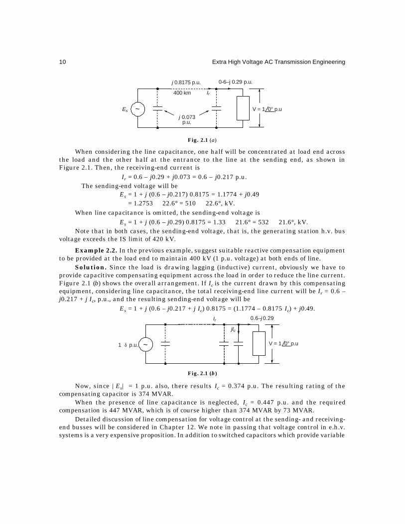
When considering the line capacitance, one half will be concentrated at load end acrossthe load and the other half at the entrance to the line at the sending end, as shown inFigure 2.1. Then, the receiving-end current is
Ir = 0.6 – j0.29 + j0.073 = 0.6 – j0.217 p.u.∴ The sending-end voltage will be
Es = 1 + j (0.6 – j0.217) 0.8175 = 1.1774 + j0.49= 1.2753 ∠ 22.6° = 510 ∠ 22.6°, kV.
When line capacitance is omitted, the sending-end voltage isEs = 1 + j (0.6 – j0.29) 0.8175 = 1.33 ∠ 21.6° = 532 ∠ 21.6°, kV.
Note that in both cases, the sending-end voltage, that is, the generating station h.v. busvoltage exceeds the IS limit of 420 kV.
Example 2.2. In the previous example, suggest suitable reactive compensation equipmentto be provided at the load end to maintain 400 kV (1 p.u. voltage) at both ends of line.
Solution. Since the load is drawing lagging (inductive) current, obviously we have toprovide capacitive compensating equipment across the load in order to reduce the line current.Figure 2.1 (b) shows the overall arrangement. If Ic is the current drawn by this compensatingequipment, considering line capacitance, the total receiving-end line current will be Ir = 0.6 –j0.217 + j Ic, p.u., and the resulting sending-end voltage will be
Es = 1 + j (0.6 – j0.217 + j Ic) 0.8175 = (1.1774 – 0.8175 Ic) + j0.49.
Fig. 2.1 (b)
Now, since |Es| = 1 p.u. also, there results Ic = 0.374 p.u. The resulting rating of thecompensating capacitor is 374 MVAR.
When the presence of line capacitance is neglected, Ic = 0.447 p.u. and the requiredcompensation is 447 MVAR, which is of course higher than 374 MVAR by 73 MVAR.
Detailed discussion of line compensation for voltage control at the sending- and receiving-end busses will be considered in Chapter 12. We note in passing that voltage control in e.h.v.systems is a very expensive proposition. In addition to switched capacitors which provide variable
~j 0.073
p.u.
j 0.8175 p.u.
400 km Ir
Es
0-6–j 0.29 p.u.
V = 1 0° p.u
~
Ir 0.6– 0.29j
1 p.u.∠δ V = 1 0° p.u
jIc

Transmission Line Trends and Preliminaries 11
capacitive reactive power to suit variation of load from no load to full load, variable inductivecompensation will be required which takes the form of thyristor-controlled reactors (TCR)which are also known as Static VAR Systems. Unfortunately, these give rise to undesirableharmonics which are injected into the line and may cause maloperation of signalling and somecommunication equipment. These problems and use of proper filters to limit the harmonicinjection will also be discussed in Chapter 12.
2.2 AVERAGE VALUES OF LINE PARAMETERSDetailed calculation of line parameters will be described in Chapter 3. In order to be able toestimate how much power a single-circuit at a given voltage can handle, we need to know thevalue of positive-sequence line inductance and its reactance at power frequency. Furthermore,in modern practice, line losses caused by I2R heating of the conductors is gaining in importancebecause of the need to conserve energy. Therefore, the use of higher voltages than may bedictated by purely economic consideration might be found in order not only to lower the currentI to be transmitted but also the conductor resistance R by using bundled conductors comprisingof several sub-conductors in parallel. We will utilize average values of parameters for lineswith horizontal configuration as shown in Table 2.1 for preliminary estimates.
When line resistance is neglected, the power that can be transmitted depends upon (a) themagnitudes of voltages at the ends (Es, Er), (b) their phase difference ,δ and (c) the total positive-sequence reactance X per phase, when the shunt caspacitive admittance is neglected.
Thus, P = Es Er sin δ /(L.x) ...(2.1)where P = power in MW, 3-phase, Es, Er = voltages at the sending-end and receiving end,
respectively, in kV line-line, δ = phase difference between Es and Er, x = positive-sequencereactance per phase, ohm/km, and L = line length, km.
Table 2.1. Average Values of Line Parameters
System kV 400 750 1000 1200Average Height, m 15 18 21 21Phase Spacing, m 12 15 18 21Conductor 2 × 32 mm 4 × 30 mm 6 × 46 mm 8 × 46 mmBundle Spacing, m 0.4572 0.4572 – –Bundle Dia., m – – 1.2 1.2r, ohm/km* 0.031 0.0136 0.0036 0.0027x, ohm/km (50 Hz) 0.327 0.272 0.231 0.231x/r 10.55 20 64.2 85.6
*At 20°C. Increase by 12.5% for 50°C.From consideration of stability, δ is limited to about 30°, and for a preliminary estimate
of P, we will take Es = Er = E.
2.3 POWER-HANDLING CAPACITY AND LINE LOSSAccording to the above criteria, the power-handling capacity of a single circuit isP = E2 sin δ /Lx. At unity power factor, at the load P, the current flowing is
I = E sin 3/δ Lx ...(2.2)

12 Extra High Voltage AC Transmission Engineering
and the total power loss in the 3-phases will amount to
p = 3I2rL = E2. sin2 δ .r/Lx2 ...(2.3)Therefore, the percentage power loss is
%p = 100 p/P = 100. sin δ .(r/x) ...(2.4)
Table 2.2. shows the percentage power loss and power-handling capacity of lines at variousvoltage levels shown in Table 2.1, for δ = 30° and without series-capacitor compensation.
Table 2.2. Percent Power Loss and Power-Handling Capacity
System kV 400 750 1000 1200
76.455.10
50= 5.2
2050
= 78.02.64
50= 584.0
6.8550
=
Lx,MWE.P /50 2=
400 670 2860 6000 8625600 450 1900 4000 5750
800 335 1430 3000 43101000 270 1140 2400 3450
1200 225 950 2000 2875
The following important and useful conclusions can be drawn for preliminary understandingof trends relating to power-handling capacity of a.c. transmission lines and line losses.
(1) One 750-kV line can normally carry as much power as four 400-kV circuits for equaldistance of transmission.
(2) One 1200-kV circuit can carry the power of three 750-kV circuits and twelve 400-kVcircuits for the same transmission distance.
(3) Similar such relations can be found from the table.
(4) The power-handling capacity of line at a given voltage level decreases with line length,being inversely proportional to line length L.From equation (2.2) the same holds for current to be carried.
(5) From the above property, we observe that if the conductor size is based on currentrating, as line length increases, smaller sizes of conductor will be necessary. Thiswill increase the danger of high voltage effects caused by smaller diameter of conductorgiving rise to corona on the conductors and intensifying radio interference levels andaudible noise as well as corona loss.
(6) However, the percentage power loss in transmission remains independent of linelength since it depends on the ratio of conductor resistance to the positive-sequencereactance per unit length, and the phase difference δ between Es and Er.
(7) From the values of % p given in Table 2.2, it is evident that it decreases as the systemvoltage is increased. This is very strongly in favour of using higher voltages if energyis to be conserved. With the enormous increase in world oil prices and the need for
Percentage, Power LossLine Length, km

Transmission Line Trends and Preliminaries 13
conserving natural resources, this could sometimes become the governing criterionfor selection of voltage for transmission. The Bonneville Power Administration (B.P.A.)in the U.S.A. has based the choice of 1150 kV for transmission over only 280 kmlength of line since the power is enormous (10,000 MW over one circuit).
(8) In comparison to the % power loss at 400 kV, we observe that if the same power istransmitted at 750 kV, the line loss is reduced to (2.5/4.76) = 0.525, at 1000 kV it is0.78/4.76 = 0.165, and at 1200 kV it is reduced further to 0.124.
Some examples will serve to illustrate the benefits accrued by using very high transmissionvoltages.
Example 2.3. A power of 12,000 MW is required to be transmitted over a distance of 1000km. At voltage levels of 400 kV, 750 kV, 1000 kV, and 1200 kV, determine:
(1) Possible number of circuits required with equal magnitudes for sending and receiving-end voltages with 30° phase difference;
(2) The currents transmitted; and
(3) The total line losses.Assume the values of x given in Table 2.1. Omit series-capacitor compensation.Solution. This is carried out in tabular form.
System, kv 400 750 1000 1200
x, ohm/km 0.327 0.272 0.231 0.231P = 0.5 E2/Lx, MW 268 1150 2400 3450
(a) No. of circuits
(=12000/P) 45 10–11 5 3–4
(b) Current, kA 17.31 9.232 6.924 5.77
(c) % power loss, p 4.76 2.5 0.78 0.584
Total power loss, MW 571 300 93.6 70
The above situation might occur when the power potential of the Brahmaputra River inNorth-East India will be harnessed and the power transmitted to West Bengal and Bihar. Notethat the total power loss incurred by using 1200 kV ac transmission is almost one-eighth thatfor 400 kV. The width of land required is far less while using higher voltages, as will be detailedlater on.
Example 2.4. A power of 2000 MW is to be transmitted from a super thermal powerstation in Central India over 800 km to Delhi. Use 400 kV and 750 kV alternatives. Suggest thenumber of circuits required with 50% series capacitor compensation, and calculate the totalpower loss and loss per km.
Solution. With 50% of line reactance compensated, the total reactance will be half of thepositive-sequence reactance of the 800-km line.
Therefore P = 0.5 × 4002/400 × 0.327 = 670 MW/Circuit at 400 kVand P = 0.5 × 7502/400 × 0.272 = 2860 MW/Circuit at 750 kV

14 Extra High Voltage AC Transmission Engineering
400 kV 750 kV
No. of circuits required 3 1
Current per circuit, kA 667/ 3 × 400 = 0.963 1.54
Resistance for 800 km, ohms 0.031 × 800 = 24.8 0.0136 × 800 = 10.88
Loss per circuit, MW 3 × 24.8 × 0.9632 = 69 MW 3 × 10.88 × 1.542
= 77.4 MW
Total power loss, MW 3 × 69 = 207 77.4
Loss/km, kW 86.25 kW/km 97 kW/km
2.4 EXAMPLES OF GIANT POWER POOLS AND NUMBER OF LINESFrom the discussion of the previous section it becomes apparent that the choice of transmissionvoltage depends upon (a) the total power transmitted, (b) the distance of transmission, (c) the %power loss allowed, and (d) the number of circuits permissible from the point of view of landacquisition for the line corridor. For example, a single circuit 1200 kV line requires a width of56 m, 3 – 765 kV require 300 m, while 6 single-circuit 500 kV lines for transmitting the samepower require 220 m-of-right-of-way (R-O-W). An additional factor is the technological know-how in the country. Two examples of similar situations with regard to available hydro-electricpower will be described in order to draw a parallel for deciding upon the transmission voltageselection. The first is from Canada and the second from India. These ideas will then be extendedto thermal generation stations situated at mine mouths requiring long transmission lines forevacuating the bulk power to load centres.
2.4.1 Canadian ExperienceThe power situation in the province of Quebec comes closest to the power situation in India, inthat nearly equal amounts of power will be developed eventually and transmitted over nearlythe same distances. Hence the Canadian experience might prove of some use in making decisionsin India also. The power to be developed from the La Grande River located in the James Bayarea of Northern Quebec is as follows : Total 11,340 MW split into 4 stations [LG–1: 1140, LG–2 : 5300, LG–3 : 2300, and LG–4: 2600 MW]. The distance to load centres at Montreal andQuebec cities is 1100 km. The Hydro-Quebec company has vast ecperience with their existing735 kV system from the earlier hydroelectric development at Manicouagan-Outardes Rivers sothat the choice of transmission voltage fell between the existing 735 kV or a future 1200 kV.However, on account of the vast experience accumulated at the 735 kV level, this voltage wasfinally chosen. The number of circuits required from Table 2.2 can be seen to be 10–11 for 735kV and 3–4 for 1200 kV. The lines run practically in wilderness and land acquisition is not asdifficult a problem as in more thickly populated areas. Plans might however change as thedevelopment proceeds. The 1200 kV level is new to the industry and equipment manufacture isin the infant stages for this level. As an alternative, the company could have investigated thepossibility of using e.h.v. dc transmission. But the final decision was to use 735 kV, ac. In 1987,a ± 450 kV h.v. d.c. link has been decided for James Bay-New England Hydro line (U.S.A.) fora power of 6000 MW.

Transmission Line Trends and Preliminaries 15
2.4.2 Indian RequirementThe giant hydro-electric power pools are located in the northern border of the country on theHimalayan Mountain valleys. These are in Kashmir, Upper Ganga on the Alakhananda andBhagirathi Rivers, Nepal, Bhutan, and the Brahmaputra River. Power surveys indicate thefollowing power generation and distances of transmission:
(1) 2500 MW, 250 km, (2) 3000 MW, 300 km, (3) 4000 MW, 400 km, (4) 5000 MW, 300 km,(5) 12000 MW over distances of (a) 250 km, (b) 450 km, and (c) 1000-1200 km.
Using the power-handling capacities given in Table 2.2 we can construct a table showingthe possible number of circuits required at differenct voltage levels (Table 2.3).
Table 2.3: Voltage Levels and Number of Circuits for Evacuating fromHydro-Electric Power Pools in India
Power, MW 2500 3000 4000 5000 12000Distance, km 250 300 400 300 250 450 1000No. of Circuits/ 3/400 4/400 6/400 6/400 12/400 20/400 48/400Voltage Level 1/750 2/750 2/750 3/750 6/750 12/750Voltage Level (70% (75%) 1/1200 2/1200 6/1000(Ac only) loaded) 4/1200
One can draw certain conclusions from the above table. For example, for powers up to5000 MW, 400 kV transmission might be adequate. For 12000 MW, we observe that 750 kVlevel for distances up to 450 km and 1200 kV for 1000 km might be used, although even for thisdistance 750 kV might serve the purpose. It is the duty of a design engineer to work out suchalternatives in order that final decisions might be taken. For the sake of reliability, it is usualto have at least 2 circuits.
While the previous discussion is limited to ac lines, the dc alternatives must also beworked out based upon 2000 Amperes per pole. The usual voltages used are ± 400 kV (1600MW/bipole), ± 500 kV (2000 MW) and ± 600 kV (2400 MW). These power-handling capacitiesdo not depend on distances of transmission. It is left as an exercise at the end of the chapter forthe reader to work out the dc alternatives for powers and distances given in Table 2.3.
2.5 COSTS OF TRANSMISSION LINES AND EQUIPMENTIt is universally accepted that cost of equipment all over the world is escalating every
year. Therefore, a designer must ascertain current prices from manufacturer of equipmentand line materials. These include conductors, hardware, towers, transformers, shunt reactors,capacitors, synchronous condensers, land for switchyards and line corridor, and so on. Generatingstation costs are not considered here, since we are only dealing with transmission in this book.In this section, some idea of costs of important equipment is given (which may be current in2005) for comparison purposes only. These are not to be used for decision-making purposes.
(1US$ = Rs.50; 1 Lakh = 100, 000; 1 Crore = 100 Lakhs = 10 Million = 107).
(a) High Voltage DC ± 400 kV Bipole
Back-to-back terminals : Rs. 50 Lakhs/MVA for 150 MVA
Rs. 40 Lakhs/MVA for 300 MVA

16 Extra High Voltage AC Transmission Engineering
Cost of 2 terminals : Rs. 40 Lakhs/MVATransmission line: Rs. 26.5 Lakhs/Circuit (cct) kmSwitchyards : Rs. 3000 Lakhs/bay
(b) 400 kV AC
Transformers : 400/220 kV AutotransformersRs. 3.7 Lakhs/MVA for 200 MVA 3-phase unit
to Rs. 3 Lakhs/MVA for 500 MVA 3-phase unit400 kV/13.8 kV Generator TransformersRs. 2 Lakhs/MVA for 250 MVA 3-phase unit
to Rs. 1.5 Lakh/MVA for 550 MVA 3-phase unit.
(c) Shunt Reactors
Non-switchable Rs. 2.6 Lakhs/MVA for 50 MVA unit to
Rs. 2 Lakhs/MVA for 80 MVA unitSwitchable Rs. 9 to 6.5 Lakhs/MVA for 50 to 80 MVA units.
Shunt Capacitors Rs. 1 Lakh/MVA
Synchronous Condensers (Including transformers) :
Rs. 13 Lakhs/MVA for 70 MVA to
Rs. 7 Lakhs/MVA for 300 MVA
Transmission Line Cost:
400 kV Single Circuit: Rs. 25 Lakhs/cct km220 kV: S/C: Rs. 13 Lakhs/cct km; D/C: Rs. 22 Lakhs/cct km.
Example 2.5. A power of 900 MW is to be transmitted over a length of 875 km. Estimatethe cost difference when using ± 400 kV dc line and 400 kV ac lines.
Solution. Power carried by a single circuit dc line = 1600 MW. Therefore,1 Circuit is sufficient and it allows for future expansion.Power carried by ac line = 0.5 E 2/xL = 0.5 × 4002/ (0.32 × 875) = 285 MW/cct.∴ 3 circuits will be necessary to carry 900 MW.DC Alternative: cost of
(a) Terminal Stations Rs. 33.5 × 10³ Lakhs
(b) Transmission Line Rs. 23 × 103 Lakhs
(c) 2 Switchyard Bays Rs. 5.8 × 10³ Lakhs Total Rs. 62.3 × 10³ Lakhs = Rs. 623 Crores
AC Alternative: Cost of
(a) 6 Switchyard Bays Rs. 17.5 × 10³ Lakhs
(b) Shunt reactors 500 MVA Rs. 1 × 10³ Lakhs
(c) Shunt capacitors 500 MVA Rs. 0.5 × 10³ Lakhs
(d) Line cost: (3 × 875 × 25 Lakhs) Rs. 65 × 103 Lakhs
Total Rs. 84 × 103 Lakhs = Rs. 840 Crores

Transmission Line Trends and Preliminaries 17
Difference in cost = Rs. 217 Crores, dc being lower than ac.(Certain items common to both dc and ac transmission have been omitted. Also, series
capacitor compensation has not been considered).
Example 2.6. Repeat the above problem if the transmission distance is 600 km.Solution. The reader can calculate that the dc alternative costs about 55 x 103 Lakhs or
Rs. 550 Crores.For the ac alternative, the power-handling capacity per circuit is increased to 285 × 875/600
= 420 MW. This requires 2 circuits for handling 900 MW.The reactive powers will also be reduced to 120 MVA for each line in shunt reactors and
switched capacitors. The cost estimate will then include:
(a) 4 Switchyard Bays Rs. 11 × 103 Lakhs
(b) Shunt reactors 240 MVA Rs. 0.6 × 10³ Lakhs
(c) Shunt capacitors Rs. 0.27 × 10³ Lakhs
(d) Line cost: 2 × 600 × 25 Lakhs Rs. 30 × 103 Lakhs
Total Rs. 41. 87 × 103 Lakhs = 418.7 Crores.The dc alternative has become more expensive than the ac alternative by about Rs.130
Crores. In between line lengths of 600 km and 875 km for transmitting the same power, thetwo alternatives will cost nearly equal. This is called the "Break Even Distance".
2.6 MECHANICAL CONSIDERATIONS IN LINE PERFORMANCE
2.6.1 Types of Vibrations and OscillationsIn this section a brief description will be given of the enormous importance which designersplace on the problems created by vibrations and oscillations of the very heavy conductorarrangement required for e.h.v. transmission lines. As the number of sub-conductors used in abundle increases, these vibrations and countermeasures and spacings of sub-conductors willalso affect the electrical design, particularly the surface voltage gradient. The mechanicaldesigner will recommend the tower dimensions, phase spacings, conductor height, sub-conductorspacings, etc. from which the electrical designer has to commence his calculations of resistance,inductance, capacitance, electrostatic field, corona effects, and all other performancecharacteristics. Thus, the two go hand in hand.
The sub-conductors in a bundle are separated by spacers of suitable type, which bringtheir own problems such as fatigue to themselves and to the outer strands of the conductorduring vibrations. The design of spacers will not be described here but manufacturers' cataloguesshould be consulted for a variety of spacers available. These spacers are provided at intervalsranging from 60 to 75 metres between each span which is in the neighbourhood of 300 metresfor e.h.v. lines. Thus, there may be two end spans and two or three subspans in the middle. Thespacers prevent conductors from rubbing or colliding with each other in wind and ice storms, ifany. However, under less severe wind conditions the bundle spacer can damage itself or causedamage to the conductor under certain critical vibration conditions. Electrically speaking, sincethe charges on the sub-conductors are of the same polarity, there exists electrostatic repulsionamong them. On the other hand, since they carry currents in the same direction, there iselectromagnetic attraction. This force is especially severe during short-circuit currents so thatthe spacer has a force exerted on it during normal or abnormal electrical operation.

18 Extra High Voltage AC Transmission Engineering
Three types of vibration are recognized as being important for e.h.v. conductors, theirdegree of severity depending on many factors, chief among which are: (a) conductor tension, (b)span length, (c) conductor size, (d) type of conductor, (e) terrain of line, (f) direction of prevailingwinds, (g) type of supporting clamp of conductor-insulator assemblies from the tower, (h) towertype, (i) height of tower, (j) type of spacers and dampers, and (k) the vegetation in the vicinity ofline. In general, the most severe vibration conditions are created by winds without turbulenceso that hills, buildings, and trees help in reducing the severity. The types of vibration are: (1)Aeolian Vibration, (2) Galloping, and (3) Wake-Induced Oscillations. The first two are presentfor both single-and multi-conductor bundles, while the wake-induced oscillation is confined to abundle only. Standard forms of bundle conductors have sub-conductors ranging from 2.54 to 5cm diameters with bundle spacing of 40 to 50 cm between adjacent conductors. For e.h.v.transmission, the number ranges from 2 to 8 sub-conductors for transmission voltages from400 kV to 1200 kV, and up to 12 or even 18 for higher voltages which are not yet commerciallyin operation. We will briefly describe the mechanism causing these types of vibrations and theproblems created by them.
2.6.2 Aeolian VibrationWhen a conductor is under tension and a comparatively steady wind blows across it, smallvortices are formed on the leeward side called Karman Vortices (which were first observed onaircraft wings). These vortices detach themselves and when they do alternately from the topand bottom they cause a minute vertical force on the conductor. The frequency of the forces isgiven by the accepted formula
F = 2.065 v/d, Hz ...(2.5)where v = component of wind velocity normal to the conductor in km/ hour, and d = diameterof conductor in centimetres. [The constant factor of equation (2.5) becomes 3.26 when v is inmph and d in inches.]
The resulting oscillation or vibrational forces cause fatigue of conductor and supportingstructure and are known as aeolian vibrations. The frequency of detachment of the Karmanvortices might correspond to one of the natural mechanical frequencies of the span, which ifnot damped properly, can build up and destroy individual strands of the conductor at points ofrestraint such as at supports or at bundle spacers. They also give rise to wave effects in whichthe vibration travels along the conductor suffering reflection at discontinuities at points ofdifferent mechanical characteristics. Thus, there is associated with them a mechanical impedance.Dampers are designed on this property and provide suitable points of negative reflection toreduce the wave amplitudes. Aeolian vibrations are not observed at wind velocities in excess of25 km/hour. They occur principally in terrains which do not disturb the wind so that turbulencehelps to reduce aeolian vibrations.
In a bundle of 2 conductors, the amplitude of vibration is less than for a single conductordue to some cancellation effect through the bundle spacer. This occurs when the conductorsare not located in a vertical plane which is normally the case in practice. The conductors arelocated in nearly a horizontal plane. But with more than 2 conductors in a bundle, conductorsare located in both planes. Dampers such as the Stockbridge type or other types help to dampthe vibrations in the subspans connected to them, namely the end sub-spans, but there areusually two or three sub-spans in the middle of the span which are not protected by thesedampers provided only at the towers. Flexible spacers are generally provided which may or

Transmission Line Trends and Preliminaries 19
may not be designed to offer damping. In cases where they are purposely designed to damp thesub-span oscillations, they are known as spacer-dampers.
Since the aeolian vibration depends upon the power imparted by the wind to the conductor,measurements under controlled conditions in the laboratory are carried out in wind tunnels.The frequency of vibration is usually limited to 20 Hz and the amplitudes less than 2.5 cm.
2.6.3 GallopingGalloping of a conductor is a very high amplitude, low-frequency type of conductor motion andoccurs mainly in areas of relatively flat terrain under freezing rain and icing of conductors. Theflat terrain provides winds that are uniform and of a low turbulence. When a conductor is iced,it presents an unsymmetrical corss-section with the windward side having less ice accumulationthan the leeward side of the conductor. When the wind blows across such a surface, there is anaerodynamic lift as well as a drag force due to the direct pressure of the wind. the two forcesgive rise to torsional modes of oscillation and they combine to oscillate the conductor with verylarge amplitudes sufficient to cause contact of two adjacent phases, which may be 10 to 15metres apart in the rest position. Galloping is induced by winds ranging from 15 to 50 km/hour,which may normally be higher than that required for aeolian vibrations but there could be anoverlap. The conductor oscillates at frequencies between 0.1 and 1 Hz. Galloping is controlledby using "detuning pendulums" which take the form of weights applied at different locations onthe span.
Galloping may not be a problem in a hot country like India where temperatures arenormally above freezing in winter. But in hilly tracts in the North, the temperatures may dipto below the freezing point. When the ice loosens from the conductor, it brings another oscillatorymotion called Whipping but is not present like galloping during only winds.
2.6.4 Wake-Induced OscillationThe wake-induced oscillation is peculiar to a bundle conductor, and similar to aeolian vibrationand galloping occurring principally in flat terrain with winds of steady velocity and low turbulence.The frequency of the oscillation does not exceed 3 Hz but may be of sufficient amplitude to causeclashing of adjacent sub-conductors, which are separated by about 50 cm. Wind speeds for causingwake-induced oscillation must be normally in the range 25 to 65 km/hour. As compared to this,aeolian vibration occurs at wind speeds less than 25 km/hour, has frequencies less than 20 Hzand amplitudes less than 2.5 cm. Galloping occurs at wind speeds between 15 and 50 km/hour,has a low frequency of less than 1 Hz, but amplitudes exceeding 10 metres. Fatigue failure tospacers is one of the chief causes for damage to insulators and conductors.
Wake-induced oscillation, also called "flutter instability", is caused when one conductoron the windward side aerodynamically shields the leeward conductor. To cause this type ofoscillation, the leeward conductor must be positioned at rest towards the limits of the wake orwindshadow of the windward conductor. The oscillation occurs when the bundle tilts 5 to 15°with respect to a flat ground surface. Therefore, a gently sloping ground with this angle cancreate conditions favourable to wake-induced oscillations. The conductor spacing to diameterratio in the bundle is also critical. If the spacing B is less than 15d, d being the conductordiameter, a tendency to oscillate is created while for B/d > 15 the bundle is found to be morestable. As mentioned earlier, the electrical design, such as calculating the surface voltagegradient on the conductors, will depend upon these mechanical considerations.

20 Extra High Voltage AC Transmission Engineering
2.6.5 Dampers and SpacersWhen the wind energy imparted to the conductor achieves a balance with the energy dissipatedby the vibrating conductor, steady amplitudes for the oscillations occur. A damping devicehelps to achieve this balance at smaller amplitudes of aeolian vibrations than an undampedconductor. The damper controls the intensity of the wave-like properties of travel of theoscillation and provides an equivalent heavy mass which absorbs the energy in the wave. Asketch of a Stockbridge damper is shown in Fig. 2.2.
A simpler form of damper is called the Armour Rod, which is a set of wires twisted aroundthe line conductor at the insulator supporting conductor and hardware, and extending forabout 5 metres on either side. This is used for small conductors to provide a change in mechanicalimpedance. But for heavier conductors, weights must be used, such as the Stockbridge, whichrange from 5 kg for conductors of 2.5 cm diameter to 14 kg for 4.5 cm. Because of the steelstrands inside them ACSR conductors have better built-in property against oscillations thanACAR conductors.
Fig. 2.2 (a) Stockbridge Damper; (b) Suspension Clamp (Courtesy: Electrical Manufacturing Co., Calcutta).
Fig. 2.3 Spacer for two-conductor bundle (Courtesy: EMC, Calcutta).
DamperMass
Steel Massenger
Cable
Centre ofGravity
ConductorDamper Clamp
Cushion Insert
Conductor
CushionAluminium AlloyRetaining Rods
Frame
(a)
(b)

Transmission Line Trends and Preliminaries 21
There are a large number of types of spacers which keep the conductors apart. Mostmodern spacers have some flexibility built into them to allow rotation of the conductor insidethem such as lining the clamps with high-strength plastic or rubber washers. Some spacers arespecially designed to act as dampers and may also take the form of heavy springs. The selectionof the spacers is also determined by the wind speed in the locality. Fig. 2.3 shows a spacer usedfor a bundle conductor.
Review Questions and Problems
1. Of the following transmission voltages (given in kV) used in the world, which onesare used in India at present: 66, 132, 169, 220, 275, 345, 400, 500–525, 735–765, 1000,1150.
2. The geography and civilization of any country can best be understood by a knowledgeof location of its rivers. In modern days, power development also depends on therivers. On an atlas, locate the following rivers in the countries listed. Note: Due tointernational disputes and wars between nations some of the rivers may not be in thecountries given, but only in the general geographic area in an atlas.
(a) Indian sub–continent (including Tibet, Pakistan, Bangladesh and Burma)—Sind,Jhelum, Ganga; Yamuna, Bhagirathi, Alakhnanda, Gandak, Gomti, Tsang-Po,Dehang, Brahmaputra, Padma, Hoogly, Narmada, Damodar, Mahanadi, Godavari,Krishna, Kali, Sharavathi, Kaveri, Vaigai, Tamraparni, Irrawaddy, Salween.
(b) Canada and U.S.—Fraser, Columbia, Slave, Mackenzie, Athabasca, TheSaskatchewans, Winnipeg, Nelson, Peace (Finlay and Parsnip), Red, St. Lawrence,St. John, Churchill, Ottawa, La Grande, Colorado, Mississippi-Missouri, Ohio,Rio Grande, Delaware, Hudson, Mohawk, Niagara.
(c) Europe, including the U.S.S.R. and Siberia—Severn, Clyde, Thames, Danube,Rhone, Rhine, Elb, Po, Seine, Ob, Volga, Dneiper, Lena, Yenesei.
(d) Other parts of the world—Yangtze, Yellow, Senju, Marude, Yalu, Nile, Zambezi,Congo (Zaire), Amazon, Itaipu, Orinaco, Makong, La Plata, Sikiang, Volta.
3. Using equations (2.1) and (2.2), draw on a graph the variation of P and I as the distanceof transmission is varied from 200 to 800 km for (a) 400 kV line, and (b) 750 kV line.U se average values for r and x given in Table 2.1. Take P = 0.5 E2/Lx. Repeat for δ =45°.
4. In the U.S.A., for transmitting a power of 10,000 MW over 285 km, a voltage of 1150kV was selected. In the U.S.S.R., for transmitting a power of 5000 MW over 800 km,the same voltage level was selected. Give your comments on the reasons this level ismost suitable and what the possible reasons are for such a choice. Discuss through%line loses by comparing with other suitable voltage classes that could have beenfound suitable.
5. Using the figures for power to be transmitted and distance given in Table 2.3, workout dc alternative for India to evacuate these powers to load centres.
6. Write brief descriptions of (a) aeolian vibration, and (b) wake-induced oscillations.Describe the measures taken to minimize the damage due to them.
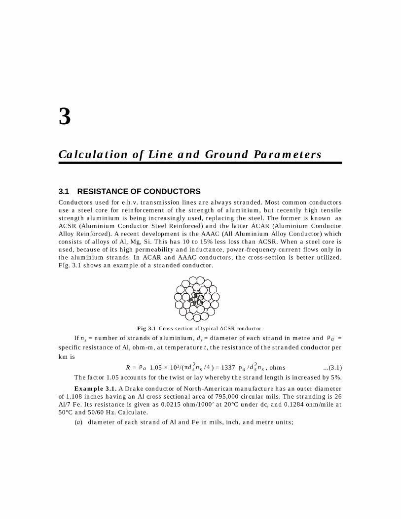
3.1 RESISTANCE OF CONDUCTORSConductors used for e.h.v. transmission lines are always stranded. Most common conductorsuse a steel core for reinforcement of the strength of aluminium, but recently high tensilestrength aluminium is being increasingly used, replacing the steel. The former is known asACSR (Aluminium Conductor Steel Reinforced) and the latter ACAR (Aluminium ConductorAlloy Reinforced). A recent development is the AAAC (All Aluminium Alloy Conductor) whichconsists of alloys of Al, Mg, Si. This has 10 to 15% less loss than ACSR. When a steel core isused, because of its high permeability and inductance, power-frequency current flows only inthe aluminium strands. In ACAR and AAAC conductors, the cross-section is better utilized.Fig. 3.1 shows an example of a stranded conductor.
Fig 3.1 Cross-section of typical ACSR conductor.
If ns = number of strands of aluminium, ds = diameter of each strand in metre and aρ =specific resistance of Al, ohm-m, at temperature t, the resistance of the stranded conductor perkm is
R = aρ 1.05 × 10³/( 4/2ss ndπ ) = 1337 ssa nd2/ρ , ohms ...(3.1)
The factor 1.05 accounts for the twist or lay whereby the strand length is increased by 5%.
Example 3.1. A Drake conductor of North-American manufacture has an outer diameterof 1.108 inches having an Al cross-sectional area of 795,000 circular mils. The stranding is 26Al/7 Fe. Its resistance is given as 0.0215 ohm/1000' at 20°C under dc, and 0.1284 ohm/mile at50°C and 50/60 Hz. Calculate.
(a) diameter of each strand of Al and Fe in mils, inch, and metre units;
3Calculation of Line and Ground Parameters
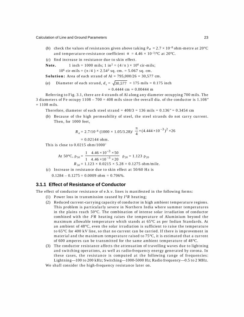
Calculation of Line and Ground Parameters 23
(b) check the values of resistances given above taking aρ = 2.7 × 10⁻⁸ ohm-metre at 20°Cand temperature-resistance coefficient α = 4.46 × 10⁻³/°C at 20°C.
(c) find increase in resistance due to skin effect.Note. 1 inch = 1000 mils; 1 in2 = ( π/4 ) × 106 cir-mils;
106 cir-mils = ( 4/π ) × 2.542 sq. cm. = 5.067 sq. cm.Solution: Area of each strand of Al = 795,000/26 = 30,577 cm.
(a) Diameter of each strand, ds = 577,30 = 175 mils = 0.175 inch
= 0.4444 cm = 0.00444 mReferring to Fig. 3.1, there are 4 strands of Al along any diameter occupying 700 mils. The
3 diameters of Fe occupy 1108 – 700 = 408 mils since the overall dia. of the conductor is 1.108"= 1108 mils.
Therefore, diameter of each steel strand = 408/3 = 136 mils = 0.136" = 0.3454 cm
(b) Because of the high permeability of steel, the steel strands do not carry current.Then, for 1000 feet,
Ra = 2.7/10–8 (1000 × 1.05/3.28)/
×××π
26)10444.4(4
23–
= 0.02144 ohm.This is close to 0.0215 ohm/1000'
At 50°C, ρ50 = 201046.41
501046.413–
3–
××+
××+ ρ20 = 1.123 ρ20
∴ R50 = 1.123 × 0.0215 × 5.28 = 0.1275 ohm/mile.(c) Increase in resistance due to skin effect at 50/60 Hz is
0.1284 – 0.1275 = 0.0009 ohm = 0.706%.
3.1.1 Effect of Resistance of ConductorThe effect of conductor resistance of e.h.v. lines is manifested in the following forms:
(1) Power loss in transmission caused by I2R heating;(2) Reduced current-carrying capacity of conductor in high ambient temperature regions.
This problem is particularly severe in Northern India where summer temperaturesin the plains reach 50°C. The combination of intense solar irradiation of conductorcombined with the I2R heating raises the temperature of Aluminium beyond themaximum allowable temperature which stands at 65°C as per Indian Standards. Atan ambient of 48°C, even the solar irradiation is sufficient to raise the temperatureto 65°C for 400 kV line, so that no current can be carried. If there is improvement inmaterial and the maximum temperature raised to 75°C, it is estimated that a currentof 600 amperes can be transmitted for the same ambient temperature of 48°C.
(3) The conductor resistance affects the attenuation of travelling waves due to lightningand switching operations, as well as radio-frequency energy generated by corona. Inthese cases, the resistance is computed at the following range of frequencies:Lightning—100 to 200 kHz; Switching—1000-5000 Hz; Radio frequency—0.5 to 2 MHz.
We shall consider the high-frequency resistance later on.

24 Extra High Voltage AC Transmission Engineering
3.1.2 Power Loss in TransmissionIn Chapter 2, average resistance values were given in Table 2.1. For various amounts of powertransmitted at e.h.v. voltage levels, the I2R heating loss in MW are shown in Table 3.1 below.The power factor is taken as unity. In every case the phase angle difference δ = 30° between Esand Er.
Table 3.1. I2R Loss in MW of E.H.V. Lines
System kV 400 750 1000 1200
Resistance, ohm/km 0.031 0.0136 0.0036 0.0027
Power Transmitted I2R Loss, MW
1,000 MW 48 25 7.8 5.842,000 96 50 15.6 11.685,000 240 125 39 29.2
10,000 480 250 78 58.4
20,000 960 500 156 116.8
We notice the vast reduction in MW loss occurring with increase in transmission voltagefor transmitting the same power. The above calculations are based on the following equations:
(1) Current: I = VP 3/ ...(3.2)
(2) Loss: p = 3I2R = P2R/V2 ...(3.3)(3) Total resistance: R = L.r, ...(3.4)where L = line length in km,and r = resistance per phase in ohm/km.(4) Total above holds for δ = 30°. For any other power-angle the loss is
p = 3I2rL = E2r sin2 δ /(L.x2) ...(3.5)where x = positive-sequence reactance of line per phase.
3.1.3 Skin Effect Resistance in Round ConductorsIt was mentioned earlier that the resistance of overhead line conductors must be evaluated atfrequencies ranging from power frequency (50/60 Hz) to radio frequencies up to 2 MHz or more.With increase in frequency, the current tends to flow nearer the surface resulting in a decreasein area for current conduction. This gives rise to increase in effective resistance due to the'Skin Effect'. The physical mechanism for this effect is based on the fact that the inner filamentsof the conductors link larger amounts of flux as the centre is approached which causes anincrease in reactance. The reactance is proportional to frequency so that the impedance tocurrent flow is larger in the inside, thus preventing flow of current easily. The result is acrowding of current at the outer filaments of the conductor. The increase in resistance of astranded conductor is more difficult to calculate than that of a single round solid conductorbecause of the close proximity of the strands which distort the magnetic field still further. It iseasier to determine the resistance of a stranded conductor by experiment at the manufacturer'spremises for all conductor sizes manufactured and at various frequencies.

Calculation of Line and Ground Parameters 25
Fig. 3.2 Variation with frequency parameter (mr) of (a) skin effect resistance ratio Rac (f)/Rdcand (b) skin effect inductance L(f)/L0, with L0 = µ0/8π, the inductance with uniform current
distribution in round conductor.
In this section, a method of estimating the ratio Rac(f)/Rdc will be described. The rigorousformulas involve the use of Bessel Functions and the resistance ratio has been tabulated orgiven in the form of curves by the National Bureau of Standards, Washington, several decadesago. Figure 3.2(a) shows some results where the ordinate is Rac/Rdc at any frequency f and the
abscissa is X = mr = 0.0636 0/Rf , where R0 is the dc resistance of conductor in ohms/mile.
W hen using SI units, X = 1.59 × 10⁻³ mRf/ , where Rm = dc resistance in ohm/metre.
Example 3.2. A Moose conductor has a resistance of 62 milli-ohm/km. Using Fig. 3.2(a),determine the highest frequency for which the graph is applicable for a round conductor.
Solution. Maximum value of X = 4 = 0.0636 √ ./ 0Rf
Now, R0 = 62 × 10–3 × 1.609 = 0.1
Therefore f = (X/0.0636)2 R0 ≈ 400 Hz.For other frequencies the functional relationship between Rac(f)/Rdc is as follows:
Let Ber (X) = L2222
8
22
4
8.6.4.24.21 XX +−
Bei (X) = L22222
10
222
6
2
2
10.8.6.4.26.4.2–
2
XXX+ ...(3.6)
B'er(X) = d Ber (X)/dX, B'ei(X) = d Bei (X)/dX
Then,dc
ac )(R
fR= 22 )](eiB[)](erB[
)(erB).(Bei)(eiB).(Ber2 XX
XXXXX′+′
′−′
...(3.7)
The Bessel Functions are tabulated and values from there must be used [see H.B. Dwight:Mathematical Tables (Dover Publications) pages 194 onwards]. The following example willillustrate the increase in resistance of a round copper conductor up to a frequency of 100 kHz.
1.5
1.4
1.3
1.2
1.1
1.0
0 1 2 3 4
1.0
0.9
0.8
0 1 2 3 4
RR
()f
dc/
LL
L(
)0
00
f/,
= /8
µπ
mr f R= 0.0636 0 mr(a) (b)(b)(a)

26 Extra High Voltage AC Transmission Engineering
Example 3.3. A round 7/0 copper conductor 0.5" (12.7 mm) in dia. has ρ = 1.7 ×10⁻⁸
ohm-m at 20°C. Calculate the variation of Rac/Rdc as a function of frequency up to 105 Hz.Solution. R0 = 1.7 × 10–8 × 1609/(π × 12.72 × 10⁻⁶/4) = 0.216 ohm/mile
∴ 0.0636/ 0R = 0.0137.We will use a logarithmic increase for frequency;
f 100 300 600 1000 3000 6000 104 3 × 10⁴ 6 × 10⁴ 105
X = 0.0137 f .137 .237 .335 .4326 .749 1.06 1.37 2.37 3.35 4.326
Rac/Rdc
3445 10
8.
1
10
8.
1
10
4.0
1
10
37.0
1
−−−− ×
+
×
+
×
+
×
+
1.0000037, 1.00004, 1.00008, 1.0008[These values are taken from N.B.S. Tables and T. and D. Reference Book (Westinghouse)].
3.2 TEMPERATURE RISE OF CONDUCTORS AND CURRENT-CARRYINGCAPACITY
When a conductor is carrying current and its temperature has reached a steady value, heatbalance requires
+
nIrradiatioSolarby
SuppliedHeatExternal
by Developed
Heat Internal2 RI
=
+
Radiation
byLost Heat
AirtoConvection
byLost Heat...(3.8)
Let Wi = I2R heating in watts/metre length of conductorWs = solar irradiation ,, ,, ,, ,,Wc = convection loss ,, ,, ,, ,,
and Wr = radiation loss ,, ,, ,, ,,Then the heat balance equation becomes
Wi + Ws = Wc + Wr ...(3.9)Each of these four terms depends upon several factors which must be written out in terms
of temperature, conductor dimensions, wind velocity, atmospheric pressure, current, resistance,conductor surface condition, etc. It will then be possible to find a relation between the temperaturerise and current. The maximum allowable temperature of an Al conductor is 65°C at present,but will be increased to 75°C . Many countries in the world have already specified the limit as75°C above which the metal loses its tensile strength. The four quantities given above are asfollows:
(1) I2R heating. Wi = I2Rm watts/metre where, Rm = resistance of conductor per metrelength at the maximum temperature.
1.0017 1.0066 1.0182 1.148 1.35 1.8

Calculation of Line and Ground Parameters 27
Rm = .201
120Rt
α+α+
with α = temperature resistance coefficient in ohm/°C and R20 = conductor resistance at20°C.
(2) Solar irradiation.Ws = sa.Is.dm watts/metre
where dm = diametre of conductor in metre, sa = solar absorption coefficient = 1 for blackbody or well-weathered conductor and 0.6 for new conductor, and Is = solar irradiation intensityin watts/m2.
At New Delhi in a summer's day at noon, Is has a value of approximately 1000-1500 W/m2.[Note: 104 calories/sq. cm/day = 4860 watts/m2](3) Convection loss.
wc = 5.73 ,./ tdvp mm ∆ watts/m2
where p = pressure of air in atmospheres, vm = wind velocity in metres/sec.,
and ∆t = temperature rise in °C above ambient = t – ta.Since 1 metre length of conductor has an area of π dm sq. m., the convection loss is
Wc = mm dvpt ....18 ∆ , watts/metre
(4) Radiation loss. This is given by Stefan-Boltzmann Law
Wr = 5.702 × 10⁻⁸ e( 44aTT − ), watts/m2
where e = relative emissivity of conductor-surface = 1 for black body and 0.5 for oxidized Alor Cu, T = conductor temperature in °K = 273 + t and Ta = ambient temperature in °K = 273 + ta.
The radiation loss per metre length of conductor is
Wr = 17.9 × 10⁻⁸ e( 44aTT − ) dm, watt/m.
Equation (3.9) for the heat balance then becomes
I2Rm + saIsdm = 18
−
+∆44
100100..9.17.. a
mmmTTdedvpt ...(3.10)
Example 3.4. A 400-kV line in India uses a 2-conductor bundle with dm = 0.0318 m foreach conductor. The phase current is 1000 Amps (500 Amps per conductor). The area of eachconductor is 515.7 mm2, ρa = 2.7 × 10⁻⁸ ohm-m at 20°C, α = 0.0045 ohm/°C at 20°. Take theambient temperature ta = 40°C, atmospheric pressure p = 1, wind velocity vm = 1 m/s, e = 0.5and neglect solar irradiation. Calculate the final temperature of conductor due only to I2Rheating.
Solution. Let the final temperature = t°C.
Then, Rm = 2.7 ×10⁻⁸ 200045.01
0045.01×+×+ t
6107.515
05.1−×
= 0.5 × 10⁻⁴ (1 + 0.0045t), ohm/mTherefore, Wt = I2Rm = 12.5 (1 + 0.0045t), watts/m
Wc = watts/m),40–(21.3)40–.(0318.0118 tt =×
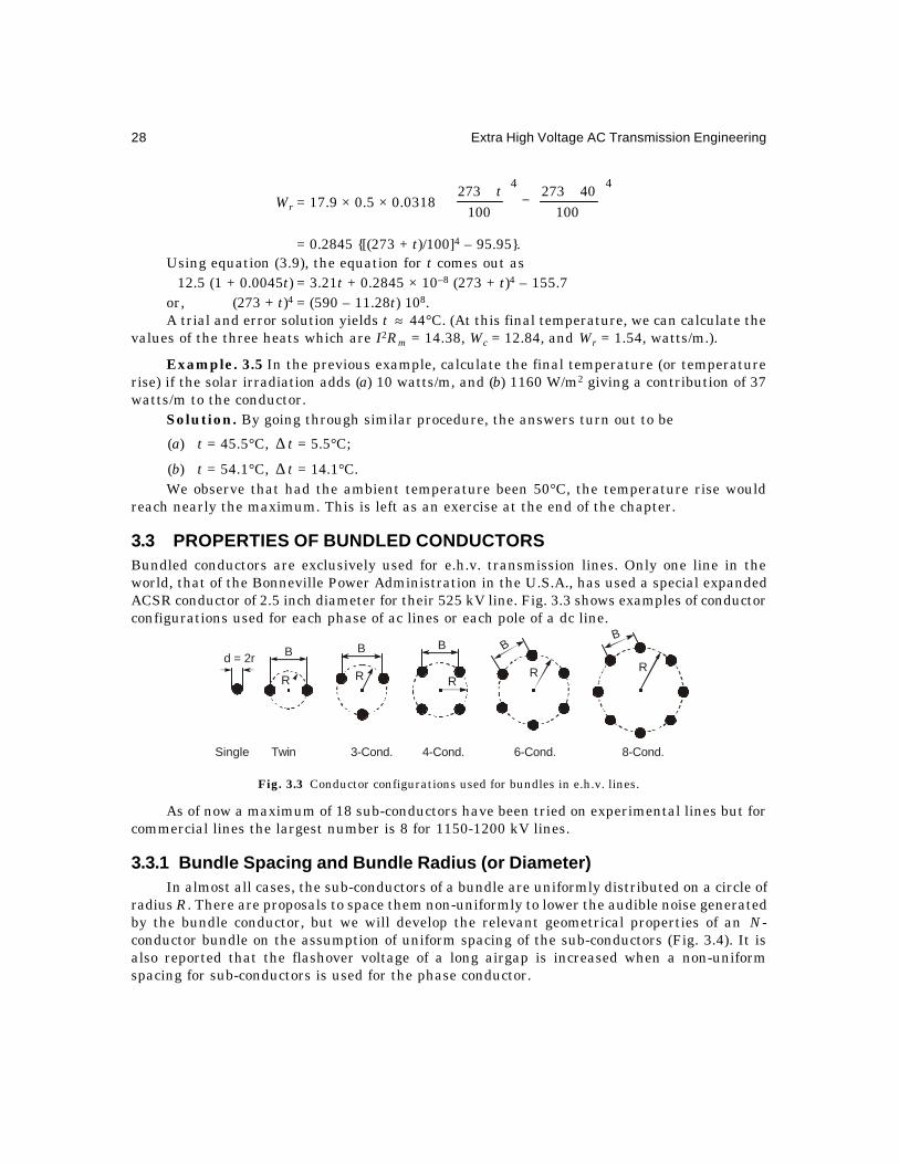
28 Extra High Voltage AC Transmission Engineering
Wr = 17.9 × 0.5 × 0.0318
+−
+ 44
10040273
100273 t
= 0.2845 [(273 + t)/100]4 – 95.95.Using equation (3.9), the equation for t comes out as
12.5 (1 + 0.0045t) = 3.21t + 0.2845 × 10⁻⁸ (273 + t)4 – 155.7or, (273 + t)4 = (590 – 11.28t) 108.A trial and error solution yields t ≈ 44°C. (At this final temperature, we can calculate the
values of the three heats which are I2Rm = 14.38, Wc = 12.84, and Wr = 1.54, watts/m.).
Example. 3.5 In the previous example, calculate the final temperature (or temperaturerise) if the solar irradiation adds (a) 10 watts/m, and (b) 1160 W/m2 giving a contribution of 37watts/m to the conductor.
Solution. By going through similar procedure, the answers turn out to be
(a) t = 45.5°C, ∆ t = 5.5°C;
(b) t = 54.1°C, ∆ t = 14.1°C.We observe that had the ambient temperature been 50°C, the temperature rise would
reach nearly the maximum. This is left as an exercise at the end of the chapter.
3.3 PROPERTIES OF BUNDLED CONDUCTORSBundled conductors are exclusively used for e.h.v. transmission lines. Only one line in theworld, that of the Bonneville Power Administration in the U.S.A., has used a special expandedACSR conductor of 2.5 inch diameter for their 525 kV line. Fig. 3.3 shows examples of conductorconfigurations used for each phase of ac lines or each pole of a dc line.
Fig. 3.3 Conductor configurations used for bundles in e.h.v. lines.
As of now a maximum of 18 sub-conductors have been tried on experimental lines but forcommercial lines the largest number is 8 for 1150-1200 kV lines.
3.3.1 Bundle Spacing and Bundle Radius (or Diameter)In almost all cases, the sub-conductors of a bundle are uniformly distributed on a circle of
radius R. There are proposals to space them non-uniformly to lower the audible noise generatedby the bundle conductor, but we will develop the relevant geometrical properties of an N-conductor bundle on the assumption of uniform spacing of the sub-conductors (Fig. 3.4). It isalso reported that the flashover voltage of a long airgap is increased when a non-uniformspacing for sub-conductors is used for the phase conductor.
d = 2r B B B B
R R RR R
B
Single Twin 3-Cond. 4-Cond. 6-Cond. 8-Cond.

Calculation of Line and Ground Parameters 29
Fig. 3.4 Bundle spacing B, and bundle radius R.
The spacing between adjacent sub-conductors is termed 'Bundle Spacing' and denoted byB. The radius of the pitch circle on which the sub-conductors are located will be called the'Bundle Radius', denoted as R. The radius of each sub-conductor is r with diameter d. The anglesub-tended at the centre by adjacent sub-conductors is (2π/N) radians, and it is readily seen that
2B
= R sin (π/N) giving R = B/2 sin (π/N) ...(3.11)
For N = 2 to 18, the following table gives (R/B) and (B/R).N = 2 3 4 6 8 12 18
R/B = 0.5 0.578 0.7071 1 1.308 1.874 2.884
B/R = 2 3 2 1 0.7654 0.5344 0.3472
3.3.2 Geometric Mean Radius of Bundle (Equivalent Radius)Except for calculating the surface voltage gradient from the charge of each sub-conductor, formost other calculations the bundle of N-sub-conductors can be replaced by a single conductorhaving an equivalent radius. This is called the 'Geometric Mean Radius' or simply the 'EquivalentRadius.' It will be shown below that its value is
req = (N.r.RN–1)1/N = r[N.(R/r)N–1]1/N = R(N.r/R)1/N ...(3.12)It is the Nth root of the product of the sub-conductor radius r', and the distance of this sub-
conductor from all the other (N – 1) companions in the bundle. Equation (3.12) is derived as follows:Referring to Fig. 3.4, the product of (N – 1) mutual distances is
π
π
π
NR
NR
NR
3sin2
2sin2sin2 ....
π
−N
NR
1sin2
=
π
π
NNR N 2
sinsin)2( 1–.... .
1–sin
π
NN
πN
4 πN
2 πN
—
R
N 21
3
BR
4
NN–1
2 π

30 Extra High Voltage AC Transmission Engineering
req = N
N
NN
NNRr
/11– 1–
sin2
sin.sin)2.(
π
ππ...(3.13)
For N = 2, req = (2rR)1/2
For N = 3, req = 3/12
3/122 )3(
32
sin.3
sin...2 rRrR =
ππ
For N = 4, req = 4/134/1
33 )4(43
sin.42
sin.4
sin...2 rRrR =
πππ
For N = 6, req = 6/15
6/155 )..6(
65
sin6
2sin.
6sin...2 RrrR =
πππ
This is equation (3.12) where the general formula is req = (N.r.RN–1)1/N.The reader should verify the result for N = 8, 12, 18.
Example 3.6 The configurations of some e.h.v. lines for 400 kV to 1200 kV are given.Calculate req for each.
(a) 400 kV : N = 2, d = 2r = 3.18 cm, B = 45 cm
(b) 750 kV : N = 4, d = 3.46 cm, B = 45 cm
(c) 1000 kV : N = 6, d = 4.6 cm, B = 12 d
(d) 1200 kV : N = 8, d = 4.6 cm, R = 0.6 m
Solution. The problem will be solved in different ways.
(a) req = Br. = (1.59 × 45)1/2 = 8.46 cm = 0.0846 m
(b) req = 4/13 ])2/45(73.14[ ×× = 21.73 cm = 0.2173 m
(c) req = [6 × 2.3 × 55.25]1/6 = 43.81 cm = 0.4381 m
Also, req = 55.2 (6 × 2.3/55.2)1/6 = 43.81 cm
(d) req = 60 (8 × 2.3/60)1/8 = 51.74 cm = 0.5174 m
We observe that as the number of sub-conductors increases, the equivalent radius ofbundle is approaching the bundle radius. The ratio req/R is (Nr/R)1/N. The concept of equivalentbundle radius will be utilized for calculation of inductance, capacitance, charge, and severalother line parameters in the sections to follow.
3.4 INDUCTANCE OF E.H.V. LINE CONFIGURATIONSFig. 3.5 shows several examples of line configuration used in various parts of the world. Theyrange from single-circuit (S/C) 400 kV lines to proposed 1200 kV lines. Double-circuit (D/C)lines are not very common, but will come into practice to save land for the line corridor. Aspointed out in chapter 2, one 750 kV circuit can transmit as much power as 4-400 kV circuitsand in those countries where technology for 400 kV level exists there is a tendency to favourthe four-circuit 400 kV line instead of using the higher voltage level. This will save on import ofequipment from other countries and utilize the know-how of one's own country. This is aNational Policy and will not be discussed further.
...
...

Calculation of Line and Ground Parameters 31
Fig. 3.5 E.h.v. line configurations used.
3.4.1 Inductance of Two ConductorsWe shall very quickly consider the method of handling the calculation of inductance of twoconductors each of external radius r and separated by a distance D which forms the basis forthe calculation of the matrix of inductance of multi-conductor configurations.
Fig. 3.6 Round conductor with internal and external flux linkages.
1 2 32 3 3 3 '
2'21
1 1 '
(a) S/C Horizontal (b) S/C L-Type (c) D/C Conventional
1 1' 1
323'2'32
(d) D/C Double Triangle (e) S/C Delta
No.1 No.2 No.3 No.4
2 2 2 23333
(4) Four-Circuit Tower
yx
r
yedy
dye
P
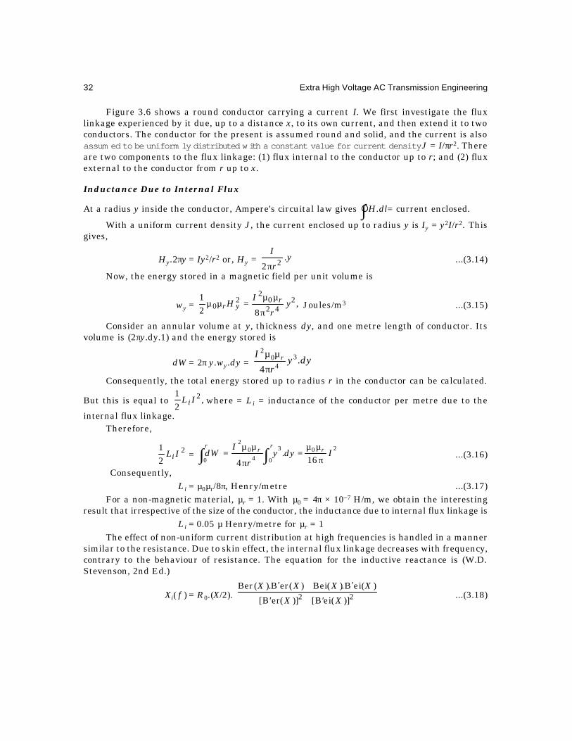
32 Extra High Voltage AC Transmission Engineering
Figure 3.6 shows a round conductor carrying a current I. We first investigate the fluxlinkage experienced by it due, up to a distance x, to its own current, and then extend it to twoconductors. The conductor for the present is assumed round and solid, and the current is alsoassum ed to be uniform ly distributed with a constant value for current density J = I/πr2. Thereare two components to the flux linkage: (1) flux internal to the conductor up to r; and (2) fluxexternal to the conductor from r up to x.
Inductance Due to Internal Flux
At a radius y inside the conductor, Ampere's circuital law gives H.dl= current enclosed.
With a uniform current density J, the current enclosed up to radius y is Iy = y2I/r2. Thisgives,
Hy.2πy = Iy2/r2 or, Hy = yr
I.
2 2π...(3.14)
Now, the energy stored in a magnetic field per unit volume is
wy = ,82
1 242
02
20 y
r
IH r
yrπ
µµ=µµ Joules/m3 ...(3.15)
Consider an annular volume at y, thickness dy, and one metre length of conductor. Itsvolume is (2πy.dy.1) and the energy stored is
dW = 2π y.wy.dy = dyyr
I r .4
34
02
πµµ
Consequently, the total energy stored up to radius r in the conductor can be calculated.
But this is equal to ,21 2ILi where = Li = inductance of the conductor per metre due to the
internal flux linkage.Therefore,
221
ILi = ∫∫ πµµ
=π
µµ=
rrr
rIdyy
r
IdW
0
203
40
2
0 16.
4...(3.16)
Consequently,Li = µ0µr/8π, Henry/metre ...(3.17)
For a non-magnetic material, µr = 1. With µ0 = 4π × 10–7 H/m, we obtain the interestingresult that irrespective of the size of the conductor, the inductance due to internal flux linkage is
Li = 0.05 µ Henry/metre for µr = 1The effect of non-uniform current distribution at high frequencies is handled in a manner
similar to the resistance. Due to skin effect, the internal flux linkage decreases with frequency,contrary to the behaviour of resistance. The equation for the inductive reactance is (W.D.Stevenson, 2nd Ed.)
Xi( f ) = R0.(X/2). 22 )](eiB[)](erB[
)(eiB.)(Bei)(erB).(Ber
XX
XXXX
′+′
′+′...(3.18)
∫
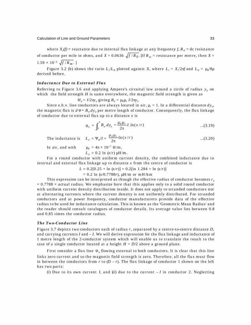
Calculation of Line and Ground Parameters 33
where Xi(f) = reactance due to internal flux linkage at any frequency f, R0 = dc resistance
of conductor per mile in ohms, and X = 0.0636 ./ 0Rf [If Rm = resistance per metre, then X =
1.59 × 10⁻³ ./ mRf ]
Figure 3.2 (b) shows the ratio Li/L0 plotted against X, where Li = Xi/2πf and L0 = µ0/8µderived before.
Inductance Due to External Flux
Referring to Figure 3.6 and applying Ampere's circuital law around a circle of radius ye onwhich the field strength H is same everywhere, the magnetic field strength is given as
He = I/2πye giving Be = µ0µr I/2πye
Since e.h.v. line conductors are always located in air, µr = 1. In a differential distance dye,the magnetic flux is d φ = Be.dye per metre length of conductor. Consequently, the flux linkageof conductor due to external flux up to a distance x is
ψe = )/(ln.2
. 0 rxIdyB rx
ree π
µµ=∫ ...(3.19)
The inductance is Le = Ψe/I = )/(ln20 rxr
πµµ
...(3.20)
In air, and with µ0 = 4π × 10–7 H/m,Le = 0.2 ln (x/r) µH/m.
For a round conductor with uniform current density, the combined inductance due tointernal and external flux linkage up to distance x from the centre of conductor is
L = 0.2[0.25 + ln (x/r)] = 0.2[in 1.284 + ln (x/r)]= 0.2 ln (x/0.7788r), µH/m or mH/km
This expression can be interpreted as though the effective radius of conductor becomes re= 0.7788 × actual radius. We emphasize here that this applies only to a solid round conductorwith uniform current density distribution inside. It does not apply to stranded conductors norat alternating currents where the current density is not uniformly distributed. For strandedconductors and at power frequency, conductor manufacturers provide data of the effectiveradius to be used for inductance calculation. This is known as the 'Geometric Mean Radius' andthe reader should consult catalogues of conductor details. Its average value lies between 0.8and 0.85 times the conductor radius.
The Two-Conductor Line
Figure 3.7 depicts two conductors each of radius r, separated by a centre-to-centre distance D,and carrying currents I and – I. We will derive expression for the flux linkage and inductance of1 metre length of the 2-conductor system which will enable us to translate the result to thecase of a single conductor located at a height H = D/2 above a ground plane.
First consider a flux line φ e flowing external to both conductors. It is clear that this linelinks zero current and so the magnetic field strength is zero. Therefore, all the flux must flowin between the conductors from r to (D – r). The flux linkage of conductor 1 shown on the lefthas two parts:
(i) Due to its own current I, and (ii) due to the current – I in conductor 2. Neglecting
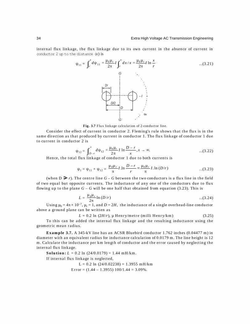
34 Extra High Voltage AC Transmission Engineering
internal flux linkage, the flux linkage due to its own current in the absence of current inconductor 2 up to the distance (x) is
ψ11 = rxIxdxId
x
r
rrx
rln
2/
200
11 ∫∫ πµµ=
πµµ=ψ ...(3.21)
Fig. 3.7 Flux linkage calculation of 2-conductor line.
Consider the effect of current in conductor 2. Fleming's rule shows that the flux is in thesame direction as that produced by current in conductor 1. The flux linkage of conductor 1 dueto current in conductor 2 is
ψ12 = ∫ ∞→πµµ=ψ
x
rD
r xx
rDId–
012 .,
–ln
2...(3.22)
Hence, the total flux linkage of conductor 1 due to both currents is
ψ1 = ψ11 + ψ12 = )/(ln.–
ln. 00 rDIr
rDI rr
πµµ≈
πµµ
...(3.23)
(when D r). The centre line G – G between the two conductors is a flux line in the fieldof two equal but opposite currents. The inductance of any one of the conductors due to fluxflowing up to the plane G – G will be one half that obtained from equation (3.23). This is
L = )/(ln20 rDr
πµµ
...(3.24)
Using µ0 = 4π × 10–7, µr = 1, and D = 2H, the inductance of a single overhead-line conductorabove a ground plane can be written as
L = 0.2 ln (2H/r), µ Henry/metre (milli Henry/km) (3.25)To this can be added the internal flux linkage and the resulting inductance using the
geometric mean radius.
Example 3.7. A 345-kV line has an ACSR Bluebird conductor 1.762 inches (0.04477 m) indiameter with an equivalent radius for inductance calculation of 0.0179 m. The line height is 12m. Calculate the inductance per km length of conductor and the error caused by neglecting theinternal flux linkage.
Solution: L = 0.2 ln (24/0.0179) = 1.44 mH/km.If internal flux linkage is neglected,
L = 0.2 ln (24/0.02238) = 1.3955 mH/kmError = (1.44 – 1.3955) 100/1.44 = 3.09%.
D/2
2r
D
– I
φe
G
G

Calculation of Line and Ground Parameters 35
We also note that GMR/outer radius = 0.0179/0.02238 = 0.8. For a round solid conductor,GMR = 0.7788 × outer radius.
3.4.2 Inductance of Multi-Conductor Lines—Maxwell's CoefficientsIn the expression for the inductance L = 0.2 ln (2H/r) of a single conductor located above aground plane, the factor P = ln (2H/r) is called Maxwell's coefficient. When several conductorsare present above a ground at different heights each with its own current, the system of n-conductors can be assumed to consist of the actual conductors in air and their images belowground carrying equal currents but in the opposite direction which will preserve the groundplane as a flux line. This is shown in Fig. 3.8.
Fig. 3.8 Multi-conductor line above ground with image conductors below ground.
The flux linkage of any conductor, say 1, consists of 3 parts in a 3-phase line, due its owncurrent and the contribution from other conductors. The self flux linkage is ψ11 = (µ0/2π) I1 ln(2H/r). We may use the geometric mean radius instead of r to account for internal flux linkageso that we write ψ11 = (µ02π) I1 ln (2H/Ds), where Ds = self-distance or GMR. For a bundle-conductor, we will observe that an equivalent radius of the bundle, equation (3.12), has to beused.
Now consider the current in conductor 2 only and the flux linkage of conductor 1 due tothis and the image of conductor 2 located below ground. For the present neglect the presenceof all other currents. Then, the flux lines will be concentric about conductor 2 and only thoselines beyond the aerial distance A12 from conductor 1 to conductor 2 will link conductor 1.Similarly, considering only the current–I2 in the image of conductor 2, only those flux linesflowing beyond the distance I12 will link the aerial conductor 1. Consequently, the total fluxlinkage of phase conductor 1 due to current in phase 2 will be
ψ12 = )/ln(2
//2 12122
022
0
1212
AIIxdxIxdxI r
IA
r
πµµ
=
−
πµµ ∫∫
∞∞
...(3.26)
The mutual Maxwell's coefficient between conductors 1 and 2 will beP12 = ln (I12/A12)
In general, it is evident that the mutual Maxwell's coefficient for the flux linkage ofconductor i with conductor j (and vice-versa) will be with i, j = 1, 2, ...n,
Pij = ln (Iij/Aij), i≠ j. ...(3.27)
H1
I1
I2I3
H2 H3
1
23
Ground
A12
I1
– I1
– I2– I3
I3I2
1
2
3
2H12H2 2H3I12
Ground

36 Extra High Voltage AC Transmission Engineering
Thus, for a system of n conductors (phases or poles) shown in Fig. 3.8, the flux-linkagematrix is
[ψ]n = nnnnnnr ILIP ][][][][
20 =πµµ
...(3.28)
where [ψ]n = [ψ1,ψ2,..., ψn]t,[In] = [I1,I2,..., In]t,
and the elements of Maxwell's coefficient matrix are
Pii = ln (2H/req) and Pji = Pij = ln (Iij/Aij), i ≠ j ...(3.29)The diagonal elements of the inductance matrix [L]nn represent the self-inductances, and
the off-diagonal elements the mutual-inductances.
3.4.3 Bundled Conductor Lines: Use of Equivalent Radius, req
In this section we will show that for a bundle conductor consistingof N sub-conductors, the denominator in the self Maxwell'scoefficient is to be taken as req of equation (3.12). This is doneunder the following basic assumptions:
(1) The bundle spacing B between adjacent sub-conductorsor the bundle radius R is very small compared to theheight H of the phase conductor above ground. Thisallows the use of 2H as the distance between any sub-conductor of the bundle and the image of all the other(N–1) sub-conductors below ground, as shown in Fig.3.9. This means that
I11 = I12 = I13 = ... = I1N = 2H(2) The total current carried by the bundle is I and that
of each sub-conductor is i = I/N.(3) Internal flux linkages are omitted, but can be included
if the problem warrants it.
Consider the flux linkage of conductor 1, which is
ψ1 =
++π
+π
+πµµ
NNR
H
NR
H
NR
HrH
NIr
1–sin2
2ln
2sin2
2ln
sin2
2ln
2ln
20
= ππππµµ
NN
NNRr
HNI
N
r
1–sin
2sin.sin.)2(
)(2ln
2 1–
N0
= eq
r
rH
I2
ln20
πµµ
...(3.30)
where req is precisely what is given in equation (3.12). The self-inductance of the entirebundle is
L = ψ1/I = )/ln(220
eqr rH
πµµ
...(3.31)
Fig. 3.9 Calculation of equivalentradius of bundle.
...
...
2H
N 12
3
N'1'
2'
3'
Ground

Calculation of Line and Ground Parameters 37
while the inductance of each subconductor will be
Lc = ψ1/i = )/ln(220
eqr rHN
πµµ
...(3.32)
which is also N times the bundle inductance since all the sub-conductors are in parallel.The Maxwell's coefficient for the bundle is Pb = ln (2H/req), as for a single conductor withequivalent radius req.
Example 3.7. The dimensions of a 3-phase 400-kV horizontal line, Fig. 3.10, are:H = 15 m, S = 11 m phase separation, conductor 2 × 3.18 cm dia, and B = 45.72 cm. Calculate.
(a) the matrix of inductances per km, for untransposed configuration, and
(b) the same when there is complete transposition.
Fig. 3.10 400-kV line for Example 3.7
Solution. req = mBr 0853.04572.00159.0. =×=P11 = P22 = P33 = ln (2 × 15/0.0853) = 5.863
P12 = P21 = P23 = P32 = ln 0664.1)/4(22
=+ SSH
P13 = P31 = ln 525.0)2/44(22
=+ SSH
(a) [L]ut = 0.2 ìH/m
mH/km863.5,0664.1,525.0
0664.1,863.5,0664.1
525.0,0664.1,863.5
= mH/km
173.1
213.0,173.1
105.0,213.0,173.1
(b)For the completely transposed line, since each phase occupies each of the 3 positionsfor 1/3 the distance, the average mutual inductance will be 0.2 (1.0664 + 1.0664 + 0.525)/3= 0.177 mH/km.
[L]t = mH/km
173.1,177.0,177.0
177.0,173.1,177.0
177.0,177.0,173.1
,,
,,
,,
=
smm
msm
mms
LLLLLLLLL
Note that the self inductance of usual e.h.v. lines is in the neighbourhood of 1 mH/km. Weobserved that as the number of sub-conductors is increased, the geometric mean radius or equivalent
H = 15m
1 2 3
11 m 11 m

38 Extra High Voltage AC Transmission Engineering
radius of bundle increases. Since req divides 2H in the logarithm, bundling will reduce the seriesinductance of a line, which will increase the power-handling capacity. Table 2.1 in Chapter 2shows this property where, as the system kV increases, the need for using more sub-conductorsis urgent from considerations of current-carrying capacity as well as reducing the voltage gradienton conductor surface. This also brings the benefit of decrease in series reactance and improvementin power-handling capacity of a single circuit. Fig. 3.5 must again be referred for details.
3.5 LINE CAPACITANCE CALCULATIONConsider two conductors of equal radii r located with their centres 2H apart, as shown inFig. 3.11. The charges on each is Q coulombs/metre and of opposite polarity. On a unit positivetest charge located at point F at a distance x from the centre of the conductor on the left withpositive charge Q, the total force exerted will be
Ef = Newtons–2
112 0
+
π xHxeQ
...(3.33)
Fig. 3.11 Single-phase line for capacitance calculation.
(This results from Gauss's Law and the reader is referred to Chapter 4 if it is not alreadyknown from previous courses devoted to Electrostatics.). Consequently, the potential differencebetween the two conductors is
V = rrH
eQ
dxxHxe
Q rH
r
–2ln)]–2/(1/1[
2 0
–2
0 π=+
π ∫ ...(3.34)
If 2H r as is usual in e.h.v. lines, V = 0e
Qπ ln (2H/r); By symmetry, the mid-plane G–G
will be at 0.5 V and the p.d. between the positive conductor and G–G is Vg = V/2.Therefore
Vg = charge positivefrom cond. of Dist.charge negativefrom cond. of Dist.
ln2
2ln
2 00 eQ
rH
eQ
π=
π ...(3.35)
2 r
F'
E'F
E'F
2 H
x
G
G

Calculation of Line and Ground Parameters 39
Since the factor ln (2H/r) multiplies the charge coefficient (Q/2πe0), which is in volts, it iscalled Mawell's Potential coefficient. We encountered the same factor in inductance calculationalso. The mid-plane G–G is an equipotential surface since the electric force is everywhereperpendicular to it as can be observed from the vector field intensity EF' at a point F', whosecomponents along G –G are equal and opposite.
We again observe that when the ground plane G – G is considered an equipotential surfacefor capacitance calculations, its effect can be considered by using an image conductor with acharge equal to the charge on the aerial conductor but of opposite polarity. From equation(3.35), we write the self potential coefficient as
Pii = ln (2H/r) ...(3.36)The mutual potential coefficients between phases are determined by placing the conductors
and their images with proper charges as shown in Fig 3.12. Following equation (3.35) thepotential of conductor 1 due to the charges Q2 and – Q2 of conductor 2 and its image will be
V12 = 120
21212
0
2
2
2
0
2 .2
)/(ln2fromDistance
–from Distanceln
2P
eQ
AIe
QQQ
eQ
π=
π=
+π...(3.37)
For a system of n conductors (phases or poles) above ground, the potential of conductorswill be
rH
eQ
AI
eQ
AI
eQ
V
AI
eQ
AI
eQ
rH
eQ
V
nn
n
n
n
nn
n
nn
2ln
2ln
2ln
2
ln2
ln2
2ln
2
02
2
0
2
1
1
0
1
1
1
012
12
0
21
0
11
π++
π+
π=
π++
π+
π=
In matrix form,
[V]n = [P]nn[Q/2πe0]n ...(3.38)
Fig. 3.12 Multi-conductor line for calculation of Maxwell's potential coefficients.
....
....
....
....
1'
2'
3'
A23A12
A13
1
2
3
2H32H22H1
I12
I13I23

40 Extra High Voltage AC Transmission Engineering
where [V]n = [V1, V2, ..., Vn]t = the potentials with respect to ground, and [Q]n = [Q1, Q2, ...,Qn]t = the conductor charges. The elements of the potential coefficient matrix are
Pii = ln (2Hi/r), Pij = ln (Iij/Aij), i ≠ j, i, j = 1, 2, ..., n ...(3.39)The capacitance matrix of the n-conductor system
[C ]nn = ][2][2 01–
0 MePe nn π=π ...(3.40)
We derived the inductance matrix for the n-conductor system to be, equation (3.28)
[L]nn = nnP ][2
0
πµ
...(3.41)
If internal flux linkages be neglected there results the important relation
[L][C ] = µ0e0[U] = ][12
Ug
...(3.42)
where [U] = unit matrix, and g = velocity of light = 3 × 10⁵ km/sec.*
Potential Coefficients for Bundled-Conductor LinesWhen each phase or pole comprises of N sub-conductors we once again arrive at the concept ofgeometric mean radius or equivalent radius of bundle req exactly in the same manner as forinductance calculations. In the self potential coefficient, equation (3.39), req will be used insteadof r. This is derived as follows, on the assumptions that
(1) the bundle dimensions B and R are small compared to line height H, and
(2) B and R are small compared to the spacing S from the centre of one phase to another.Fig. 3.9 is again referred from which, with each conductor having a charge q = Q/N per
unit length, the potential of conductor 1 is
V1 =
π++
π+
π+
πN
NR
H
NR
H
NR
HrH
NeQ
1–sin2
2ln
2sin2
2ln
sin2
2ln
2ln
12 0
L
= 02 e
Qπ ln (2H/req)
Thus, Pii = ln (2H/req). (3.43)For calculating the mutual potential coefficients we can assume that the total bundle
charge is concentrated at the centre of the bundle conductor, or else use the two assumptionsabove that the bundle dimensions are small compared to H and S.
Example 3.8. Calculate the capacitance matrix of the 3-phase 400 kV line of Example 3.7.Solution. (a) For the untransposed configuration, the matrix of Maxwell's potential
coefficients was found to be
[P]ut =
863.5,0664.1,525.0
0664.1,863.5,0664.1
525.0,0664.1,863.5
*In this book, the symbol g denotes light velocity or velocity of e.m. wave in free space, instead of thestandard symbol c. This is because c is reserved for denoting capacitance per unit length.

Calculation of Line and Ground Parameters 41
Its inverse is
[M]ut = 1–][ utP =
176.0,0298.0–,0104.0–
0298.0–,1805.0,0298.0–
0104.0–,0298.0–,176.0
The resulting capacitance matrix will be
[C ] = 2πe0[M] = eFarad/metr],[18
10 9–M
[C ]ut = nF/km
77.9,65.1–,58.0–
65.1–,02.10,65.1–
58.0–,65.1–,77.9
(b) For the completely transposed line,
[C ] = nF/km29.1–
andnF/km85.9,
,,
,,
,,
==
m
s
smm
msm
mms
ccwith
ccccccccc
We observe that the self capacitance of e.h.v. lines is in the neighbourhood of 10 nF/km.All the self-capacitance coefficients are positive while the mutual capacitance coefficients arenegative. For the horizontal configuration of phases, the centre-phase has a slightly higherself-capacitance (capacitance to ground) due to the increase in number of dielectric lines offorce terminating on it. The negative sign in mutual-capacitance follows from the physicalconsideration that a charge of one polarity placed on a conductor induces a charge of oppositepolarity on another, i.e., the two conductors form the positive and negative electrodes of acapacitor.
Bundling increases the capacitance from that of a single conductor having the same cross-sectional area because of the equivalent bundle radius which depends on the bundle radiuswhich is larger than the conductor radius. We will consider these aspects under voltage-gradientcalculations in a later section.
3.6 SEQUENCE INDUCTANCES AND CAPACITANCESThe use of Symmetrical Components for analysing 3-phase problems has made it possible tosolve very extensive network problems. It depends upon obtaining mutually-independentquantities from the original phase quantities that have mutual interaction. Following thisconcept, we will now resolve the inductances, capacitances, charges, potentials etc., intoindependent quantities by a general method. This procedure will be used for many types ofexcitations other than power-frequency later on. The basis for such transformations is to impresssuitable driving functions and obtain the resulting responses.
Inductance Transformation to Sequence QuantitiesWe observed that for a fully-transposed 3-phase ac line, the flux-linkage equation is
[ψ]3 = [L]33 [I]3 ...(3.44)

42 Extra High Voltage AC Transmission Engineering
The inductance matrix is symmetric for a transposed line for which the symmetrical-components theory will be used. For zero-sequence, the currents in the 3 phases are equal andin phase so that I1 = I2 = I3 = I0. The resulting flux linkage is.
[ψ0] = 00 )2(
1
1
1
1
1
1
,,
,,
,,
ILLI
LLL
LLL
LLL
ms
smm
msm
mms
+
=
Consequently, the inductance offered to zero-sequence currents isL0 = Ls + 2Lm ...(3.45)
When positive-sequence currents are impressed,I1 = Im sin wt, I2 = Im sin (wt – 120°) and I3 = Im sin (wt + 120°)
[ψ1] = m
smm
msm
mms
I
wt
wt
wt
LLL
LLL
LLL
°+
°−
)120(sin
)120(sin
sin
,,
,,
,,
= mms ILLwtwt
wt)(
)120sin(
)120sin(
sin
−
°+°−
Hence, the inductance offered to positive-sequence currents isL1 = Ls – Lm ...(3.46)
Similarly, for negative-sequence currents, the inductance is alsoL2 = Ls – Lm ...(3.47)
Sequence Capacitances
In a similar manner, we can evaluate the zero-, positive-, and negative-sequence capacitancesby re-writing equation (3.38) as
[Q] = 2πe0[P]–1[V] = [C][V] ...(3.48)For zero-sequene voltages, [V0] = [1, 1, 1] V, and we obtain
C0 = Cs + 2Cm ...(3.49)For positive-sequence voltages, [V+] = [sin wt, sin (wt – 120°), sin (wt + 120°)] V, and C1 =
Cs – Cm. Similarly, C2 = Cs – Cm for negative-sequence voltages.From the above resolution of phase inductances into sequence inductances, and the
capacitances, we can observe the following properties which are very important for modellingof transmission lines.
(1) The zero-sequence inductance L0 is higher than the self inductance Ls, while the positiveand negative sequence inductances are lower than Ls.
(2) The converse holds for capacitances since Cm is a negative quantity.C0 < Cs and, C1 and C2 > Cs.
(3) From equations (3.45) and (3.46), the self and mutual inductances can be found fromthe sequence inductances.
Ls = )–(31
and)2(31
1010 LLLLL m ==+ ...(3.50)

Calculation of Line and Ground Parameters 43
(4) Similarly, Cs = )–(31
and)2(31
1010 CCCCC m =+ ...(3.51)
Fig. 3.13 shows representative models of transmission lines used for system study onNetwork Analysers or Digital Computers. It is easy to impress zero-sequence and positive-sequence voltages and currents and measure the responses in a practical test setup.
Fig. 3.13 Model of transmission lines for TNA study and Digital-Computer Calculation.
The sequence inductances and capacitances can be obtained from the phase quantities ina very general manner by matrix diagonalization procedure which will be described in the nextsection. Referring to the symmetrical component theory, the phase quantities are transformedto symmetrical components by the matrix multiplication
2
1
0
VVV
=
c
b
a
VVV
aaaa
2
2
1
1
111
31
...(3.52)
where a = 1 ∠ 120°.The converse of combining the symmetrical components is carried out through the matrices
c
b
a
VVV
=
2
1
0
2
2
1
1
111
VVV
aaaa ...(3.53)
These follow the original relations formulated by Dr. C.L. Fortescue as far back as 1915.We now denote
[T ] =
=
aaaaT
aaaa
2
21–
2
2
1
1
111
31
][and
1
1
111
...(3.54)
If now we carry out the multiplications [T ]–1 [L] [T ] and [T ]–1 [C] [T ] for a completelytransposed line, the result is (multiply and verify)
[T ]–1 [L] [T ] =
2
2
2
2
1
1
111
,,
,,
,,
1
1
111
31
aa
aa
LLL
LLL
LLL
aa
aa
smm
msm
mms
Ground
L – Ls mr
Cm
Cs

44 Extra High Voltage AC Transmission Engineering
=
+
ms
ms
ms
LLLL
LL
–
,–
,2
...(3.55)
The diagonal elements are the inductances for zero-sequence, positive-sequence andnegative-sequence networks.
Similarly,
[T ]–1 [C ] [T ] =
+
ms
ms
ms
CCCC
CC
–
,–
,2
...(3.56)
Such a general procedure is very convenient for de-coupling mutually-interacting quantitiesand then combining them suitably. For a general problem encountered with e.h.v. transmissionlines, they are given the generic name 'Modes of Propagation'.
3.7 LINE PARAMETERS FOR MODES OF PROPAGATIONThe sequence parameters given in the previous section apply to steady-state conditions anduse phasor algebra. The quantity a = 1 ∠120° = – 0.5 + j0.866 is a complex number. This is notalways convenient when solving equations encountered with wave propagation on the phase orpole conductors which are characterized by (a) velocity of propagation, (b) attenuation, and(c) surge impedance. Following the ideas propounded by Dr. Fortescue, the waves on multi-conductor lines can also be resolved into 'modes of propagation'. The transformation matrix[ T ] and its inverse [ T ]–1 have to be evaluated for a given problem through standard set of ruleswhich eventually diagonalize the given matrix of inductances, capacitances, resistances, surgeimpedances, and other parameters which govern the propagation characteristics. For a fully-transposed line, analytical expressions in closed form can be obtained for the transformationmatrix and its inverse using real numbers. But for untransposed lines the evaluation of [ T ] and[ T ]–1 can also be carried case by case when numerical values for the inductances, etc. aregiven. These will be discussed in detail below.
3.7.1 Diagonalization ProcedureThe resolution of mutually-interacting components of voltage, current, charge, or energy inwaves propagating on the multi-conductors depends upon diagonalization of the n × n impedancematrix. A general procedure is given here while their application to Radio Noise, SwitchingSurges, etc, will be discussed in later chapters when we consider these problems individually.
First consider the diagonalization of the inductance matrix of a transposed line
[L] =
smm
msm
mms
LLLLLLLLL
,,
,,
,,
The following steps have to be followed for diagonalization.
Step 1. We evaluate the 'characteristic roots' or 'eigenvalues' (λ) of the given matrixaccording to the determinantal equation

Calculation of Line and Ground Parameters 45
|λ[ U ] – [L]| = 0, which gives 0
–,–,
–,–,–
–,–,–
=
λ−
λ
λ
smm
msm
mms
LLL
LLL
LLL
...(3.57)
This gives λ3 – 3Lsλ2 + 0)23–(–)–(3 32322 =+λ mmssms LLLLLL
or, (λ – Ls – 2Lm) (λ – Ls + Lm)2 = 0 ...(3.58)The three eigenvalues are
λ1 = Ls + 2Lm, λ2 = Ls – Lm, λ3 = Ls – Lm ...(3.59)Step 2. For each of these eigenvalues in turn, we evaluate the 'eigenvector' [x], which is a
column matrix, according to the equation.[ U ] λn – [L] [x] = [0] ...(3.60)
Considering λ1 = Ls + 2Lm, there results the explicit equation
λ1[ U ] – [L]
3
2
1
xxx
= Lm
=
0
0
0
2,1–,1–
1–,2,1–
1–,1–,2
3
2
1
xxx
,
which in turn yields the three equations for x1, x2, x3 to be
=+=+=
02––
0–2–
0––2
321
321
321
xxxxxxxxx
...(3.61)
By choosing x1 = 1, there results x2 = x3 = x1 = 1. These corresponding eigenvector is [1, 1,1]t with the normalized form [1, 1, 1]t (1/√3).
By following a similar procedure for λ2 = Ls – Lm, there results
λ2[U] – [L]
3
2
1
yyy
= – Lm .
0
0
0
1,1,1
1,1,1
1,1,1
3
2
1
=
yyy
The three equations for y1, y2, y3 are all equal to y1 + y2 + y3 = 0. Once again letting y1 =1, we have y2 + y3 = – 1. Now we have an infinite number of choices for the values of y2 and y3,and we make a judicial choice for them based on practical engineering considerations andutility.
As a first choice, let y2 = 0. Then y3 = – 1. The resulting eigen-vector and its normalizedform are
1–
0
1
2
1and
1–
0
1
Since the third eigenvalue λ3 is also the same as λ2, we obtain the same equations for thecomponents of the eigenvector which we can designate as[z1, z2, z3]t. By choosing z1 = 1 and z3= 1, we obtain z2 = – 2. The third eigenvector and its normalized form are
[1, –2, 1]t and (1/√6) [1, – 2, 1]t.

46 Extra High Voltage AC Transmission Engineering
Step 3. Formulate the complete 3 × 3 eigenvector matrix or in general, n × n for the neigenvalues and call it the inverse of the transformation matrix [T]–1. For the problem underconsideration.
[T ]–1 = 6/1
1,2–,1
3–,0,3
2,2,2
√
√√
√√√
...(3.62)
Step 4. The transformation matrix [T] will be
[T ] = 6/1
1,3–,2
2–,0,2
1,3,2
√
√√
√
√√
...(3.63)
which turns out to be the transpose of [T ]–1.Their determinant is – 6.
Step 5. The given inductance matrix is diagonalized by the relation
[T ]–1 [L] [T ] = ][
–
,–
,2
λ=
+
ms
ms
ms
LLLL
LL
...(3.64)
This is a diagonal matrix whose elements are equal to the three eigenvalues, which mightbe seen to be the same as the sequence inductances presented to the voltage and current. Butnow they will be called the inductances for the three modes of propagation of electromagneticenergy of the waves generating them.
3.7.2 Interpretation of the EigenvectorsWe observe that the eigenvector corresponding to the first eigenvalue λ1 = Ls + 2Lm consists of[1, 1, 1], which can be interpreted as follows:
In the first mode of behaviour (or travel of all quantities on the three conductors), thevoltages, currents, charges, and accompanying energies are all equal on the three conductors.Also, they are all of the same sign or polarity. In this mode of propagation, the return currentflows in the ground and the resulting attenuation of energy etc., are high because of groundresistance. It is usually called the 'Line-to-Ground' mode of propagation or the 'homopolar'mode.
The eigenvector [1, 0, –1] corresponds to the second eigenvalue λ2 = Ls – Lm. In this casethe propagation can be seen to take place between the outer phase-conductors only, with thecentre phase being idle. Also, because this is a closed system, involving the two outer phases,ground is not involved in propagation so that attenuation is lower than in the line-to-groundmode. The second mode is called 'Line-to-Line Mode of the 1st kind', or simply 'phase-phase'mode.
The last eigenvector is [1, – 2, 1] corresponding to the repeated eigenvalue λ3 = λ2 = Ls –Lm. We observe that these eigenvectors have depended upon the choice made by us for therelative values of the components of the eigenvector in step 2 of the diagonalization procedure.There are infinite set of such values for the eigenvector components, and the choicerecommended here is felt to be the most convenient from the point of view of interpretation of

Calculation of Line and Ground Parameters 47
the physical mechanism of behaviour of the several quantities of interest in the wave-propagationphenomenon involving the three phase-conductors and ground. The eigenvector [1, –2, 1] canbe interpreted by noting that the outer phases form the 'go' for the current and the centre-phase the 'return'. Once again the system is closed if we assume charges of + 1 and + 1 on theouters and – 2 on the centre phase. Therefore, ground is not involved in the propagation in thismode. It is called the 'Line-to-Line Mode of the 2nd kind', or the 'inter-phase mode'.
Fig. 3.14 Pictorial representation of conditions of modes of propagation on 3-phase line.
These three modes can be represented pictorially as shown in Figure 3.14. Once themutually-interacting quantities are resolved into the three independent modes of propagation,in a manner identical to symmetrical-component analysis of which we are familiar, the behaviourof all quantities in each mode can be analyzed and the phase quantities obtained finally by theinverse procedure. In general, resolution into modes requires premultiplication by [T]–1 of thevoltages, currents, and charges on the phase conductors, while combining the modal quantitiesto obtain phase quantities requires pre-multiplication of the modal voltages, currents, chargesand other responses to these by [T], the transformation matrix.
The concept of modes of propagation is very useful for:
(a) design of carrier equipment for speech and protection where the attenuation of signalsand their distortion is of primary concern in determining the transmitter and receiverpowers;
(b) propagation of switching and lightning surges on the lines which cause over-voltagesand control the design of insulation clearances; and
(c) radio-interference levels generated by corona pulses on the phase-coductors whichpropagate on the conductors over a ground plane.
In the above illustration, the diagonalization procedure was applied to the matrix ofinductances of a transposed line. A similar diagonalization of the capacitance matrix for thefully-transposed line will yield the same transformation matrices. In this case, the resultingeigen-values for both inductance and capacitance are equal to the zero-, positive-, and negative-sequence quantities obtained from Fortescue's transformation using phasors in thetransformation matrix. Here, we have used only real numbers to effect the diagonalizationprocedure. The resulting [T] and [T]–1 are called 'Modified Clarke Transformation' matricesafter the eminent lady engineer Dr. Edith Clarke, who is also known for her γ−βα – or
0−β−α components of Machines Theory.
3.7.3 Velocities of Propagation for the Modes in Transposed Lines
When working with phase quantities, eq. (3.42) gave [L] [C] = 21
g[U] where g = velocity of e.m.
wave propagation, which is equal to velocity of light in a medium with µr = 1 and er = 1. [g = 1/
+1 +1 +1+1 0 –1 +1 –2 +1
Mode 1 Mode 3Mode 2

48 Extra High Voltage AC Transmission Engineering
00eµ ]. Now, consider the effect of pre-multiplying equation (3.42) by [ T ]–1 and post-multiplyingby [T]:
[ T ]–1 [L] [ C ] [ T ] = [ T ]–1 [L] [ T ] [T]–1 [ C ] [ T ]
= [ T ]–1 [ U ] [ T ] ][1122 U
gg= ...(3.65)
i.e.,
+
+
ms
ms
ms
ms
ms
ms
CCCC
CC
LLLL
LL
–
,–
,2
–
,–
,2
=
1
1
112g
==
==++2
11
200
/1)–)(–(
/1)2)(2(givesThis
gCLCCLLand
gCLCCLL
msms
msms...(3.66)
This shows that the velocities of propagation of waves in all three modes are equal to thevelocity of light. This is the case when ground-return inductance is not taken into account.Usually, in the first or line-to-ground mode (homopolar mode) inductance of ground returnreduces the velocity of propagation of that modal component to about 2 ~ 2.5 × 10⁵ km/s (nearly70-85% of g) as will be discussed after we evaluate the ground-return inductance in Section 3.8.
3.7.4 Untransposed Line: Modes of PropagationThe eigenvalues and eigenvectors resulting in transformation matrix and its inverse for anuntransposed line must be worked out on a case-by-case basis using the numerical values ofthe inductance and capacitance. No general expressions can be given although the generalprogramme for the diagonalization is the same as outlined before. Thus, a digital computer canhandle any type of matrix diagonalization. We will illustrate the procedure through an example.
Example 3.9. The inductance and capacitance matrices for the 400-kV horizontal linewere worked out in Examples 3.7 and 3.8. Diagonalize the capacitance matrix of the untransposedline.
Solution. [C]ut = nF/km
77.9,65.1–,58.0–
65.1–,02.10,65.1–
58.0–,65.1–,77.9
Step 1. |λ [U] – [C]| = 77.9–,65.1,58.0
65.1,02.10–,65.1
58.0,65.1,77.9–
λ
λ
λ
= λ3 – 29.65 λ2 + 285.46 λ – 896.67 = 0The eigenvalues are λ1 = 11.9755, λ2 = 10.35, λ3 = 7.2345. Note that the characteristic
roots are now distinct.
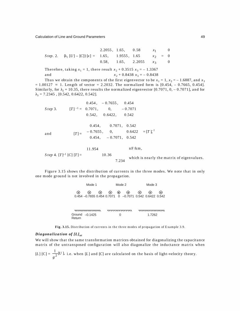
Calculation of Line and Ground Parameters 49
Step. 2. λ1 [U] – [C] [x] =
=
0
0
0
2055.2,65.1,58.0
65.1,9555.1,65.1
58.0,65.1,2055.2
3
2
1
xxx
Therefore, taking x1 = 1, there result x2 + 0.3515 x3 = – 1.3367and x2 + 0.8438 x3 = – 0.8438Thus we obtain the components of the first eigenvector to be x1 = 1, x2 = – 1.6887, and x3
= 1.00127 ≈ 1. Length of vector = 2.2032. The normalized form is [0.454, – 0.7665, 0.454].Similarly, for λ2 = 10.35, there results the normalized eigenvector [0.7071, 0, – 0.7071], and forλ3 = 7.2345 , [0.542, 0.6422, 0.542].
Step 3. [T] –1 =
542.0,6422.0,542.0
7071.0–,0,7071.0
454.0,7655.0–,454.0
and [T] = 1–][
542.0,7071.0–,454.0
6422.0,0,7655.0–
542.0,7071.0,454.0
tT=
Step 4. [T]–1 [C] [T] = s.eigenvalue ofmatrix thenearly iswhich
nF/km,
234.7
36.10
954.11
Figure 3.15 shows the distribution of currents in the three modes. We note that in onlyone mode ground is not involved in the propagation.
Fig. 3.15. Distribution of currents in the three modes of propagation of Example 3.9.
Diagonalization of [L]ut
We will show that the same transformation matrices obtained for diagonalizing the capacitancematrix of the untransposed configuration will also diagonalize the inductance matrix when
[L] [C] = ],[12
Ug
i.e. when [L] and [C] are calculated on the basis of light-velocity theory.
0.454 0.454 0.542 0.6422 0.5420.7071–0.7655 –0.70710
Mode 1 Mode 3Mode 2
GroundReturn
–0.1425 0 1.7262

50 Extra High Voltage AC Transmission Engineering
We observe that
[ T ]–1 [L] [ T ] [ T ]–1 [ C ] [ T ] = ][12
Ug
(3.67)
so that [ T ]–1 [L] [ T ] = 21
g[ T ]–1 [ C ] [ T ]–1 = 1–
2][
1 λg
(3.68)
The three eigenvalues of [L] areµ1 = 1/g2λ1,µ2 = 1/g2 λ2 and µ3 = 1/g2 λ3 (3.69)
Example 3.10. The eigenvalues of the capacitance matrices are 11.954 × 10⁻⁹ F/km, 10.36× 10⁻⁹ F/km, and 7.234 × 10⁻⁹ F/km.
Therefore, the eigenvalues of the inductance matrix will turn out to be
µ1 = 1076
1
10954.11)103(
19–25 =
××× Henry/km = 0.93 mH/km.
µ2 = mH/km0725.14.932
1
1036.10)103(
19–25 ==
×××
and µ3 = mH/km536.1651
1
10234.7)103(
19–25
==×××
Example 3.11. Taking the inductance matrix [L]ut of example 3.7 and the transformationmatrix [ T ] and its inverse [ T ]–1 from example 3.9, show that [ T ]–1 [L]ut [ T ] is diagonalized andthe eigenvalues are nearly µ1, µ2, µ3 obtained in example 3.10.
Solution.
×
542.,7071.–,454.
6422.,0,7655.–
542.,7071.,454.
173.1,213.,105.
213.,173.1,213.
105.,213.,173.1
542.,6422.,542.
7071.–,0,7071.
454.,7655.–,454.
= mH/km,
535.1,0,0
0,068.1,0
0,0,92.0
which check with µ1, µ2, µ3. (Calculated on hand calculator)
3.8 RESISTANCE AND INDUCTANCE OF GROUND RETURNUnder balanced operating conditions of a transmission line, ground-return currents do notflow. However, many situations occur in practice when ground currents have important effecton system performance. Some of these are:
(a) Flow of current during short circuits involving ground. These are confined to singleline to ground and double line to ground faults. During three phase to ground faultsthe system is still balanced;
(b) Switching operations and lightning phenomena;

Calculation of Line and Ground Parameters 51
(c) Propagation of waves on conductors;
(d) Radio Noise studies.The ground-return resistance increases with frequency of the current while the inductance
decreases with frequency paralleling that of the resistance and inductance of a conductor. In allcases involving ground, the soil is inhomogeneous and stratified in several layers with differentvalues of electrical conductivity. In this section, the famous formulas of J.R. Carson (B.S.T.J.1926) will be given for calculation of ground resistance and inductance at any frequency in ahomogeneous single-layer soil. The problem was first applied to telephone transmission but wewill restrict its use to apply to e.h.v. transmission lines.
The conductivity of soils has the following orders of magnitude: 10° mho/metre for moistsoil, 10–1 for loose soil, 10–2 for clay, and 10–3 for bed rock.
Fig. 3.16 Geometrical parameters for calculation of ground-return resistance and inductance.
Figure 3.16 describes the important parameters involved in the calculation showing twoconductors i and j above ground together with their images. We take
cs = soil conductivity in mho/m,f = frequency of current, Hz,
G = 1.7811, Euler's number, µ0 = 4π × 10–7 H/m,Iij = distance of conductor j from image of conductor i, metre,θij = arc tan [Xij/(Hi + Hj)], radians
The most important parameter involved in the calculation is
Fij = Iij sfc02πµ ...(3.70)For usual e.h.v. configurations, Fij < 1.[When c.g.s. units are used, Iij is in cm, and cs is also in c.g.s. e.m. units. To convert ohm/
m into c.g.s. units, the multiplying factor is 10-–11. Then, Fij = ]8 2sij fcI π
Having calculated Fij, the ground resistance and inductance areRg = 8πf Jr. 10–4, ohm/km ...(3.71)
Xij
Hi
Hi
Hj
Hj
Iij
J
J'
i
i'
θ ij

52 Extra High Voltage AC Transmission Engineering
and Lg = 4.Ji.10–4, Henry/km ...(3.72)where Jr and Ji are calculated as follows:
Jr = 2122422
121
5.0)/2(ln..5.08
)1( WWTFGSS ijij +−θ++π
− ...(3.73)
Ji = 0.25 + 0.5 (1 – S4). ln (2/G Fij) – 0.5 θij T4 – 8π
S2
+ 431 5.0–)(2
1WWW + ...(3.74)
There are several quantities above, (S, T, W), which are given by Carson by the followinginfinite series when Fij < 1. For most calculations, only two or three leading terms will besufficient as will be shown by an example of a horizontal 400-kV line.
S2 = ijk
ijk
kk
kkF θ+
++∑ +∞
=2)12cos(
)!22()!12(1
)2/.()1(– )12(2
0...(3.75)
T2 = same as S2 with cosine changed to sine ...(3.76)
S4 = ij
kijk
kk
kkF
θ++
∑∞
=)4(cos
)!2()!1(1
2)1(–
41–
1...(3.77)
T4 = same as S4 with cosine changed to sine ...(3.78)
W1 = ijk
ijk
kk
kF θ
−∑∞
=)3–4(cos
)14...(5.3.11
)1(– 222)1–4(1–
1...(3.79)
W2 = 1.25 S2, W4 = 3
5 4S...(3.80)
W3 = ijk
ijk
kk
kF θ
+∑∞
=)1–4(cos
)14...(531
)1(– 22)1–4(1–
1...(3.81)
The important and interesting properties of Rg and Lg for a- 3-phase line are illustrated bytaking an example of the horizontal 400-kV line. These properties come out to be
[Rg] ≈ Rg
≈
1,1,1
1,1,1
1,1,1
][and
1,1,1
1,1,1
1,1,1
gg LL ...(3.82)
Example 3.12. Figure 3.17 shows all major dimensions of a 400-kV line. Calculate thematrices of ground-return resistance and inductance per km at f = 1 kHz for cs = earth conductivity= 10–2mho/m.
Solution. The frequency of 1 kHz is useful for switching-surge propagation studies. Therequired parameters are:
θ12 = θ23 = arc tan (11/26) = 0.4014 radian.θ13 = arc tan (22/26) = 0.7025 radian.θ11 = θ22 = θ33 = 0. I12 = 30 m, I13 = 34 m.
Fij: F11 = 0.234, F12 = 0.27, F13 = 0.306

Calculation of Line and Ground Parameters 53
Fig. 3.17. Dimensions of 400 kV line for example 3.12
Self resistances and inductances: θij = 0.
S2 = 00685.0!4!3
12234.0
–!2
12234.0
62
≈+
T2 = 0,W2 = 1.25 S2 = 0.00856
S4 = .negligibleis.0.negligible,62
117.044
4WT =
×
W1 = 00028.05.3
234.0,0043.0
3.1
234.02
3
32
3=== W
Therefore
Jr = 22
0086.000215.0–
234.07811.12
ln00685.05.08
+
×××+
π
= 0.4
Ji = 0.25 + 0.5 × 1.61 – 2
0046.000685.0
8+×
π
= 1.055Therefore
Rii = 8π × 103 ×10–4 × 0.4 = 1 ohm/kmLii = 4 × 1.055 × 10–4 = 0.422 mH/km
Mutual between 1 and 2 (outer and inner)
Calculations yield Jr = 0.3983 ≈ 0.4 and Ji = 0.952Therefore R12 = R23 = 1 ohm/km, L12 = L23 = 0.38 mH/km
13
I12 I13 I23
13 θ12
θ23θ13
1 2 3
11 11
...

54 Extra High Voltage AC Transmission Engineering
Mutual between 1 and 3 (outer and outer)
Jr = 0.3925, Ji = 0.89, giving R13 ≈ 1 ohm/km andL13 = 0.356 mH/km.
∴ [Rg] = ohm/km
1,1,1
1,1,1
1,1,1
and
[Lg] = mH/km
422.0,38.0,356.0
38.0,422.0,38.0
356.0,38.0,422.0
The mutual inductances are quite close to an average value of(0.422 × 3 + 0.38 × 4 + 0.356 × 2)/9 = 0.39 mH/km
We see that the resistance and inductance of ground return are given approximately as
[Rg] = ohm/km1where,
1,1,1
1,1,1
1,1,1
=
gg RR
and [Lg] = mH/km.39.0where,
1,1,1
1,1,1
1,1,1
=
gg LL
We will denote
[D] =
1,1,1
1,1,1
1,1,1
...(3.83)
Then, [Rg] = Rg [D], and [Lg] = Lg [D] ...(3.84)
This property will be used throughout the book whenever groundreturn effects are to beconsidered.
Diagonalization of [D]
It is interesting to observe the properties of [D] by diagonalizing it. The 3 eigenvalues come outto be λ1 = 3, λ2 = λ3 = 0. One set of [T] and [T]–1 which will diagonalize [D] turn out to be exactlythe same as Clarke's Modified Transformation, equations (3.62) and (3.63), as can be workedout by the reader. Also,
[T]–1 [D] [T] = 6
1
1,3–,2
2–,0,2
1,3,2
1,1,1
1,1,1
1,1,1
1,2–,1
3–,0,3
2,2,2
6
1√
√√√
√√×
√√√√√

Calculation of Line and Ground Parameters 55
=
λλ
λ=
3
2
1
000
000
003
...(3.85)
We could have applied this property for diagonalizing the matrices of [L]t and [C]t of thetransposed line instead of the lengthy procedure in step 1 of Section. 3.7 for finding the threeeigenvalues or characteristic roots. Observe that
[L]t = ][])[–(
,,
,,
,,
DLULLLLLLLLLLL
mms
smm
msm
mms
+=
...(3.86)
Any transformation matrix which diagonalizes [D] will also diagonalize (Ls – Lm) [U] whichis already in diagonalized form.
Complete Line Parameters with Ground Return
We can now combine the resistances, inductances and capacitances of the phase conductorswith those of ground return to formulate the complete line-parameters for a transposed line.
(a) ResistanceThe conductor resistance matrix is [Rc] = Rc[ U ]Ground-return resistance matrix [Rg] = Rg [ D ]
Therefore
[R] = [Rc] + [Rg] = Rc[U] + Rg[D] =
++
+
gcgg
ggcg
gggc
RRRRRRRRRRRR
,,
,,
,,
...(3.87)
(b) Inductance
[Lc] = ][][)(
,,
,,
,,
DLULLLLLLLLLLL
mms
smm
msm
mms
+−=
...(3.88)
[Lg] = Lg[D]
∴ [L] = [Lc] + [Lg] = (Ls – Lm) [U] + (Lg + Lm) [D] ...(389)
(c) Capacitance[C] = (Cs – Cm) [U] + Cm (D) ...(3.90)
Diagonalization of any of these matrices is easily carried out through [T] and [T]–1 ofClarke's modified transformation matrices.
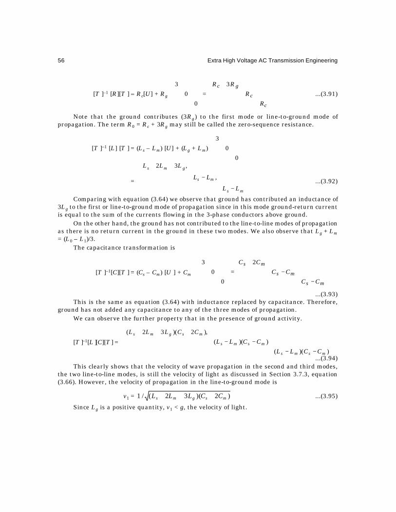
56 Extra High Voltage AC Transmission Engineering
[T ]–1 [R][T ] = Rc[U] + Rg
+=
c
c
gc
RR
RR 3
0
0
3
...(3.91)
Note that the ground contributes (3Rg) to the first mode or line-to-ground mode ofpropagation. The term R0 = Rc + 3Rg may still be called the zero-sequence resistance.
[T ]–1 [L] [T ] = (Ls – Lm) [U] + (Lg + Lm)
0
0
3
=
−
−
++
ms
ms
gms
LL
LL
LLL
,
,32
...(3.92)
Comparing with equation (3.64) we observe that ground has contributed an inductance of3Lg to the first or line-to-ground mode of propagation since in this mode ground-return currentis equal to the sum of the currents flowing in the 3-phase conductors above ground.
On the other hand, the ground has not contributed to the line-to-line modes of propagationas there is no return current in the ground in these two modes. We also observe that Lg + Lm= (L0 – L1)/3.
The capacitance transformation is
[T ]–1[C][T ] = (Cs – Cm) [U ] + Cm
−−
+=
ms
ms
ms
CCCC
CC 2
0
0
3
...(3.93)This is the same as equation (3.64) with inductance replaced by capacitance. Therefore,
ground has not added any capacitance to any of the three modes of propagation.We can observe the further property that in the presence of ground activity.
[T ]–1[L ][C][T ] =
−−−−
+++
))((
))((
),2)(32(
msms
msms
msgms
CCLLCCLL
CCLLL
...(3.94)This clearly shows that the velocity of wave propagation in the second and third modes,
the two line-to-line modes, is still the velocity of light as discussed in Section 3.7.3, equation(3.66). However, the velocity of propagation in the line-to-ground mode is
v1 = )2)(32(/1 msgms CCLLL +++ ...(3.95)
Since Lg is a positive quantity, v1 < g, the velocity of light.

Calculation of Line and Ground Parameters 57
Example 3.13. A 400-kV line (Example 3.7) gave the following inductance matrix
[L]t = mH/km
173.1,177.0,177.0
177.0,173.1,177.0
177.0,177.0,173.1
Take (Cs + 2Cm) = (1/g2) (Ls + 2Lm)–1 and (Cs – Cm) (Ls – Lm) = 1/g2. The ground returncontributes 0.39 mH/km as calculated in Example 3.12. Calculate the velocities in the threemodes.
Solution. Cs + 2Cm = (1/g2)[(1.173 + 2 × 0.177) × 10–3]–1 = 527.1101 3
2g
Ls + 2Lm + 3Lg = 2.697 × 10⁻³
∴ (Ls + 2Lm +3Lg) (Cs + 2Cm) = 1.7662/g2 = (1.329/g)2
and v1 = g/1.329 = 0.7524g = 2.2572 × 10⁵ km/sec.The velocity of propagation in the line-to-ground mode is now 75.24% of light velocity.
Equivalent Circuit of Line Model for Network Studies
From equations (3.91) and (3.92), we obtain the quantitiesR0 = Rc + 3Rg, R1 = Rc, L0 = Ls + 2Lm + 3Lg, and L1 = Ls – Lm ...(3.96)
Fig. 3.18 Line model with ground-return parameters included.
The ground-return resistance is thenRg = (R0 – R1)/3 ...(3.97)
and there also resultsLg + Lm = (L0 – L1)/3 ...(3.98)
The quantities R0 and L0 can be considered as the zero-sequence quantities while R1 andL1 are positive-sequence quantities obtained under symmetrical component concept of
C C0 – 3
1
I1
I2
I3
I1 2 3+ I + I
L1R1
B
B'
L L – 2
0 1R – R3
0 1C – 2C3
0 1
A
A'

58 Extra High Voltage AC Transmission Engineering
Fortescue. Using these, a line model can be constructed similar to Figure 3.13. This is shownin Figure 3.18.
The three lines are represented by their positive-sequence quantities R1 and L1. Theground-return part constitutes Rg and (Lg + Lm) which are denoted as (R0 – R1)/3, and (L0 – L1)/3 respectively. The capacitance network consists of a Y-connected set equal to Cs = (C0 + 2C1)/3 and a ∆-connected set of Cm = (C0 – C1)/3. The ∆-connected set may be converted to anequivalent Y if necessary each leg having a capacitance of 3Cm = (C0 – C1). Such a representationof a line section has been used for setting up miniature models on a Transient Network Analyzerfor switching-surge studies and in mathematical models for computation of transient performanceof transmission lines using the Digital Computer.
The reader can prove that the voltage drop from A to A' is(Rc + Rg) + s(Ls + Lg) I1(s) + Rg + (Lm + Lg)s I2(s) + Rg + (Lm + Lg)s I3(s) ...(3.99)This is left as an exercise at the end of the chapter.
Review Questions and Problems
1. A Moose conductor has the following details—Outer dia = 31.8 mm. Area of Al = 515.7mm2. Calculate the resistance of 1 km of a double-Moose bundled conductor at 50°Cgiven that ρa = 2.7 × 10⁻⁸ ohm-m at 20°C and temperature resistance coefficient of A1= 4.46 × 10⁻³/°C. (Increase length by 5% for stranding.)
2. The closest conductor to Moose of North-American manufacture is Bluejay with area= 1.113 × 10⁶ cir-mil, outer dia = 1.259". Its resistance is listed in tables of conductorsas 0.0166 ohm/1000 feet at 20°C for dc and 0.0941 ohm/mile at 50°C and 50/60 Hz.(a) Verify these values.
(b) Find % increase due to skin effect.
3. A 750 kV line has the details given below. Calculate the temperature rise of theconductor under given conditions. Conductor–4 × 0.03 m ACSR (area = 954,000 cir-mils). Power carried 2000 MW. ρa = 2.7 × 10⁻⁸ ohm-m at 20°C, α = 0.0045 ohm/°C,ambient ta = 45°C, e = 0.5, p = 1, v = 1.2 m/s, solar irradiation 1 kW/m2, sa = 0.8.
4. A 3-phase 750 kV horizontal line has minimum height of 12 m, sag at midspan = 12 m.Phase spacing S = 15 m. Conductors are 4 × 0.035 m with bundle spacing ofB = 0.4572 m. Calculate per kilometre:
(a) The matrix of Maxwell's Potential coefficients for an untransposed configuration.
(b) The inductance and capacitance matrices for untransposed and transposedconfigurations.
(c) The zero-, positive-, and negative-sequence inductances and capacitances fortransposed line.
(d) The ground-return resistance and inductance matrices at 750 Hz taking ρs = 100ohm-metre.For calculation take Hav = Hmin + Sag/3.

Calculation of Line and Ground Parameters 59
5. Repeat problem 3.4 for a 1150-kV delta configuration of the 3-phases with averageheight of 18 m for the lower conductors, 36 m for the top conductor, and spacing of 24m between bottom conductors. Bundle radius = 0.6 m and conductor size = 6 × 0.046m diameter. f = 1000 Hz and ρs = 50 ohm-metre.
6. Diagonalize the matrix
[D] = .
111
111
111
Give eigenvalues and eigen-vector matrices.
7. Discuss the convenience offered by using modes of propagation and possible uses ofthis technique.
8. The capacitance matrix of a 750-kV horizontal configuration line is
[C] = nF/km
20.1045.1–35.0–
45.1–45.10,45.1–
35.0–45.1–,20.10
(a) Find the 3 eigenvalues of the matrix, (λ1, λ2, λ3).
(b) Diagonalize the matrix by evaluating suitable transformation matrix [T] and itsinverse [T ]–1.
(c) Then prove that
[T ]–1 [C] [T ] =
λ
λ
λ
3
2
1
9. In problems 3.4 and 3.5 calculate the charging current supplied. Assume fulltransposition and place all the capacitance at the line entrance across the source. L =400 km.
10. In Fig. 3.18 show that the voltage drop from A to B and B' to A add to
(Rc + Rg) + s(Ls + Lg) I1 + (Rg + sLm + sLg) I2 + (Rg + sLm + sLg) I3.
where s = the Laplace-Transform operator.11. (a) Using the transformation matrices for diagonalizing the matrix [D], prove without
multiplying, that the same transformation matrices will diagonalize the inductanceor capacitance matrices of a fully-transposed line of the type.
[L] =
smm
msm
mms
LLL
LLL
LLL
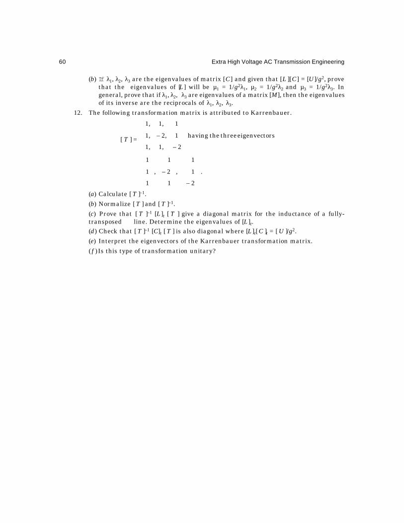
60 Extra High Voltage AC Transmission Engineering
(b) If λ1, λ2, λ3 are the eigenvalues of matrix [C] and given that [L ][C] = [U]/g2, provethat the eigenvalues of [L] will be µ1 = 1/g2λ1, µ2 = 1/g2λ2 and µ3 = 1/g2λ3. Ingeneral, prove that if λ1, λ2, λ3 are eigenvalues of a matrix [M], then the eigenvaluesof its inverse are the reciprocals of λ1, λ2, λ3.
12. The following transformation matrix is attributed to Karrenbauer.
[ T ] = rseigenvectothreethehaving
2–,1,1
1,2–,1
1,1,1
.
2–
1
1
,
1
2–
1
,
1
1
1
(a) Calculate [ T ]–1.
(b) Normalize [ T ] and [ T ]–1.
(c) Prove that [ T ]–1 [L]t [ T ] give a diagonal matrix for the inductance of a fully-transposed line. Determine the eigenvalues of [L]t.(d) Check that [ T ]–1 [C]t [ T ] is also diagonal where [L]t[ C ]t = [ U ]/g2.
(e) Interpret the eigenvectors of the Karrenbauer transformation matrix.
( f ) Is this type of transformation unitary?

4.1 ELECTROSTATICSConductors used for e.h.v. transmission lines are thin long cylinders which are known as 'linecharges'. Their charge is described in coulombs/unit length which was used for evaluating thecapacitance matrix of a multiconductor line in Chapter 3. The problems created by charges onthe conductors manifest themselves as high electrostatic field in the line vicinity from powerfrequency to TV frequencies through audio frequency, carrier frequency and radio frequency(PF, AF, CF, TVF). The attenuation of travelling waves is also governed in some measure bythe increase in capacitance due to corona discharges which surround the space near theconductor with charges. When the macroscopic properties of the electric field are studied, theconductor charge is assumed to be concentrated at its centre, even though the charge isdistributed on the surface. In certain problems where proximity of several conductors affectsthe field distribution, or where conducting surfaces have to be forced to become equipotentialsurfaces (in two dimensions) in the field of several charges it is important to replace the givenset of charges on the conductors with an infinite set of charges. This method is known as theMethod of Successive Images. In addition to the electric-field properties of long cylinders, thereare other types of important electrode configurations useful for extra high voltage practice inthe field and in laboratories. Examples of this type are sphere-plane gaps, sphere-to-spheregaps, point-to-plane gaps, rod-to-plane gaps, rod-rod gaps, conductor-to-tower gaps, conductor-to-conductor gap above a ground plane, etc. Some of these types of gaps will also be dealt within this chapter which may be used for e.h.v. measurement, protection, and other functions.The coaxial-cylindrical electrode will also be discussed in great detail because of its importancein corona studies where the bundle of N sub-conductors is strung inside a 'cage' to simulate thesurface voltage gradient on the conductors in a setup which is smaller in dimensions than anactual outdoor transmission line.
4.1.1 Field of a Point Charge and Its PropertiesThe properties of electric field of almost all electrode geometries will ultimately depend on thatof a point charge. The laws governing the behaviour of this field will form the basis for extendingthem to other geometries. Consider Figure 4.1 which shows the source point S1 where a pointcharge + Q coulombs is located. A second point charge q coulomb is located at S2 at a distancer metre from S1. From Coulomb's Law, the force acting on either charge is
4Voltage Gradients of Conductors

62 Extra High Voltage AC Transmission Engineering
F = 204/. reeqQ rπ , Newton ...(4.1)
1200 )([ −µ= ge = mFmF /84194.8/36/1000 µµ=µµπ
re = relative permittivity of the medium = 1 in air]
Fig. 4.1 Point charge Q and force on test charge q.
Where q is very small )0( →q , we define the electric field produced by Q at the location of q as
E = 20
04/)/( reeQqFLim r
qπ=
→, Newton/Coulomb ...(4.2)
The condition 0→q is necessary in order that q might not disturb the electric field of Q.Equation (4.2) may be re-written as
))(4( 02 Eeer rπ = QDr =π 24 ...(4.3)
Here we note that 24 rπ = surface are of a sphere of radius r drawn with centre at S1. The
quantity D = Eee r0 is the dielectric flux density. Thus, we obtain Gauss's Law which states
that 'the surface integral of the normal component of dielectric flux density over a closedsurface equals the total charge in the volume enclosed by the surface'. This is a general relationand is valid for all types of electrode geometries.
Some important properties of the field of a point charge can be noted:
(a) The electric field intensity decreases rapidly with distance from the point chargeinversely as the square of the distance, )/1( 2rQ ∝ .
(b) E is inversely proportional to )/1.( rr eEe ∝ .
(c) The potential of any point in the field of the point charge Q, defined as the work doneagainst the force field of Q in bringing q from ∞ to S2, is
ψ = ∫ ∫∞ ∞
π=−
π=−
r r
rr reeQ
r
dree
QEdr
144 0
20
, volt ...(4.4)
(d ) The potential difference between two points at distances r1 and r2 from S1 will be
ψ 12 =
−
π 210
114 rree
Q
r, volt ...(4.5)
For a positive point charge, points closer to the charge will be at a higher positivepotential than a further point.
(e) The capacitance of an isolated sphere is
C = ,4/ 0 reeQ rπ=ψ Farad ...(4.6)
rS1 S2 F1qQ
F

Voltage Gradients of Conductors 63
This is based on the assumption that the negative charge of – Q is at infinity.These properties and concepts can be extended in a straightforward manner to apply to
the field of a line charge and other electrode configurations.
Example 4.1. A point charge Q = 10–6 coulomb (1 µC) is kept on the surface of a conductingsphere of radius r = 1 cm, which can be considered as a point charge located at the centre of thesphere. Calculate the field strength and potential at a distance of 0.5 cm from the surface of thesphere. Also find the capacitance of the sphere, 1=ε r .
Solution. The distance of S2 from the centre of the sphere S1 is 1.5 cm.
E =
×××
π×π −−− 42126 105.110
361000
410
= 10 –6/(0.25 × 10–13)= 40 × 106 V/m = 40 MV/m = 400 kV/cm
ψ = E.r = 600 kV [using equations 4.2 and 4.4]
C = Free r µµ=π 111.14 0 with r = 0.01.
Example 4.2. The field strength on the surface of a sphere of 1 cm radius is equal to thecorona-inception gradient in air of 30 kV/cm. Find the charge on the sphere.
Solution. 30 kV/cm = 3000 kV/m = 3 × 10⁶ V/m.
3 × 106 =
××
π×π −− 412
0 101036
10004Q
= 9 × 10¹³Q0
giving Q0 = 3.33 × 10⁻⁸ coulomb = 0.033 µC.The potential of the sphere is
V = 3 × 106 × 10–2 = 30 kV.
4.2 FIELD OF SPHERE GAPA sphere-sphere gap is used in h.v. laboratories for measurement of extra high voltages and forcalibrating other measuring apparatus. If the gap spacing is less than the sphere radius, thefield is quite well determined and the sphere-gap breaks down consistently at the same voltagewith a dispersion not exceeding ±3%. This is the accuracy of such a measuring gap, if otherprecautions are taken suitably such as no collection of dust or proximity of other groundedobjects close by. The sphere-gap problem also illustrates the method of successive images usedin electrostatics.
Figure 4.2 shows two spheres of radii R separated by a centre-centre distance of S, withone sphere at zero potential (usually grounded) and the other held at a potential V. Since bothspheres are metallic, their surfaces are equipotentials. In order to achieve this, it requires aset of infinite number of charges, positive inside the left sphere at potential V and negativeinside the right which is held at zero potential. The magnitude and position of these chargeswill be determined from which the voltage gradient resulting on the surfaces of the sphere ona line joining the centres can be determined. If this exceeds the critical disruptive voltage, aspark break-down will occur. The voltage required is the breakdown voltage.

64 Extra High Voltage AC Transmission Engineering
Fig. 4.2 The sphere gap.
Consider two point charges Q1 and Q2 located with a separation D, Figure 4.3. At a pointP(x, y) with coordinates measured from Q1, the potentials are as follows:
Potential at P due to Q1 =22
110
1 with1
4yxr
reQ
+=π
Potential at P due to Q2 =22
220
2 )(with1
4yxDr
reQ
+−=π
Fig. 4.3 Point charge Q1 and sphere of radius R.
The total potential at P is VP = )//(4
12211
0
rQrQe
+π .
If this is to be zero, then Q2/Q1 = – r2/r1 ... (4.7)This clearly shows that Q1 and Q2 must be of opposite polarity.
From (4.7), 21
22 /rr = ,/
)( 21
2222
22
QQyx
yxD=
+
+− giving
2
2
212 )/(1
yQQ
Dx +
−− = 22
122
122 )/(1/)/( QQQQD − ...(4.8)
This is an equation to a circle in the two-dimensional plane and is a sphere in three-dimensional space.
R = )/(1/)/( 21212 QQQQD − ...(4.9)
This requires Q2 to be less than Q1 if the denominator is to be positive. The centre of thezero-potential surface is located at (S1, 0), where
S1 = RQQ
QQD2
1212 )/(1/ =− ...(4.10)
V V1 = V2 = 0
RR
S
V = O
RQ2
D
S1
Q1
P x, y( )
S2
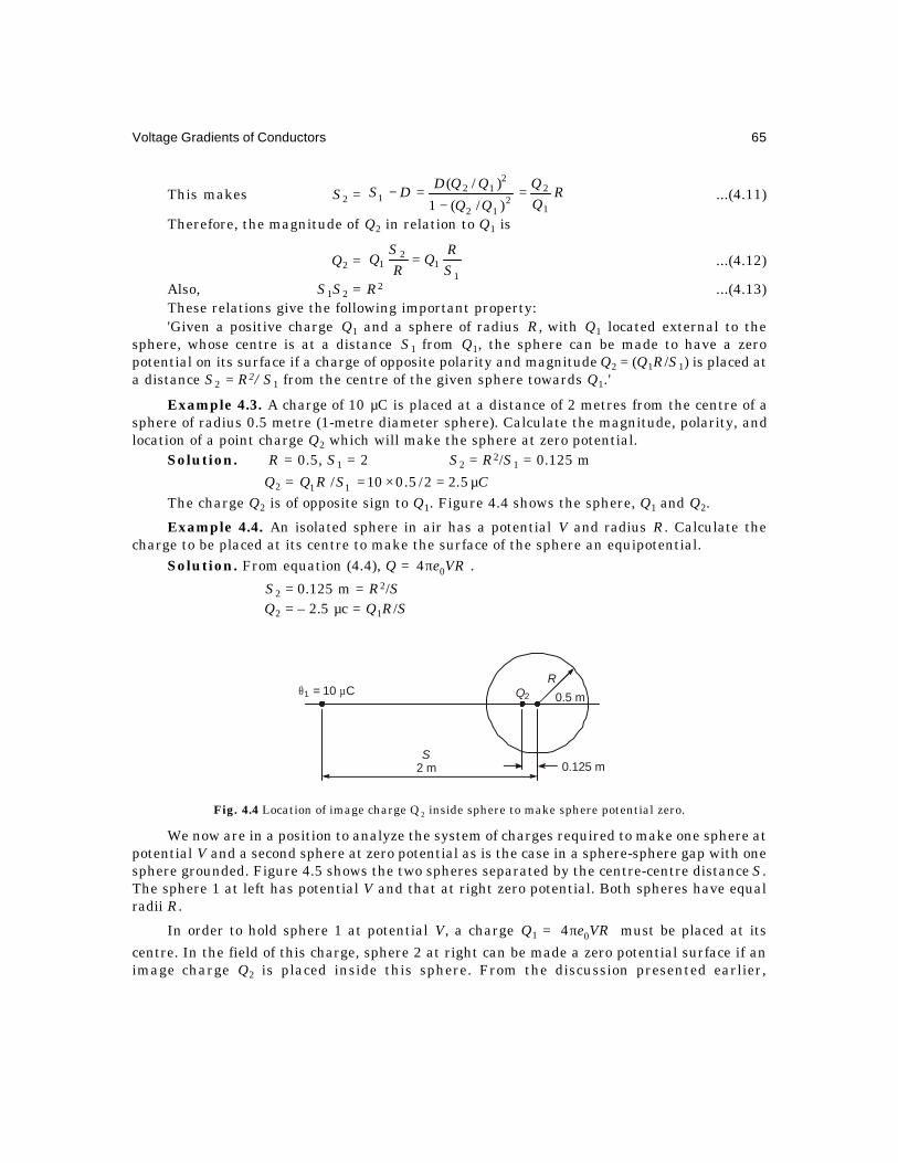
Voltage Gradients of Conductors 65
This makes S2 = RQQ
QQQQDDS
1
22
12
212
1)/(1
)/( =−
=− ...(4.11)
Therefore, the magnitude of Q2 in relation to Q1 is
Q2 =1
12
1 SR
QR
SQ = ...(4.12)
Also, S1S2 = R2 ...(4.13)These relations give the following important property:'Given a positive charge Q1 and a sphere of radius R, with Q1 located external to the
sphere, whose centre is at a distance S1 from Q1, the sphere can be made to have a zeropotential on its surface if a charge of opposite polarity and magnitude Q2 = (Q1R/S1) is placed ata distance S2 = R2/S1 from the centre of the given sphere towards Q1.'
Example 4.3. A charge of 10 µC is placed at a distance of 2 metres from the centre of asphere of radius 0.5 metre (1-metre diameter sphere). Calculate the magnitude, polarity, andlocation of a point charge Q2 which will make the sphere at zero potential.
Solution. R = 0.5, S1 = 2 ∴ S2 = R2/S1 = 0.125 m
Q2 = CSRQ µ=×= 5.22/5.010/ 11
The charge Q2 is of opposite sign to Q1. Figure 4.4 shows the sphere, Q1 and Q2.
Example 4.4. An isolated sphere in air has a potential V and radius R. Calculate thecharge to be placed at its centre to make the surface of the sphere an equipotential.
Solution. From equation (4.4), Q = VRe04π .
S2 = 0.125 m = R2/SQ2 = – 2.5 µc = Q1R/S
Fig. 4.4 Location of image charge Q 2 inside sphere to make sphere potential zero.
We now are in a position to analyze the system of charges required to make one sphere atpotential V and a second sphere at zero potential as is the case in a sphere-sphere gap with onesphere grounded. Figure 4.5 shows the two spheres separated by the centre-centre distance S.The sphere 1 at left has potential V and that at right zero potential. Both spheres have equalradii R.
In order to hold sphere 1 at potential V, a charge Q1 = VRe04π must be placed at its
centre. In the field of this charge, sphere 2 at right can be made a zero potential surface if animage charge Q2 is placed inside this sphere. From the discussion presented earlier,
θ µ = 10 C1 Q2
R0.5 m
0.125 mS 2 m

66 Extra High Voltage AC Transmission Engineering
Q2 = – Q1R/S and S2 = R2/S, as shown in Figure 4.5. However, locating Q2 will disturb thepotential of sphere 1. In order to keep the potential of sphere 1 undisturbed, we must locate animage charge )/( 221 SSRQQ' −−= inside sphere 1 so that in the field of Q2 and 'Q1 the potential
of sphere 1 is zero leaving its potential equal to V due to Q1. The charge 'Q1 is located at
)/( 22
1 SSRS' −= from Q1 (centre of sphere 1). It is now easy to see that the presence of 'Q1 will
disturb the potential of sphere 2. An image charge )/( 112''' SSRQQ −−= is called for inside
sphere 2 located at )/( 12
2'' SSRS −= from the centre of sphere 2.
Fig. 4.5. Location of successive image charges to maintain spheres at potentials V and zero.
Successive image charges will have to be suitably located inside both spheres.The sequence of charges and their locations can be tracked in a tabular form.
−=
−=−==
−−=
−−=−−=−=
−=−=−=
−−=
−−=−−=π=
.etc)/(
),/(),/(,/
2)sphere ofcentre(From
.etc),/(
),/(),/(,/Q
etc.),/(),/(),/(
1)sphere ofcentre(From
.etc),/(
)./(),/(,4
12
2
12
212
22
2
112
11211212
22
122
122
1
221
22122101
"'"'
""''
"'"'"'
"""'''
""''"'
"""'
''"'
SSRS
SSRSSSRSSRS
SSRQQ
SSRQQSSRQQSRQ
SSRSSSRSSSRS
SSRQQ
SSRQQSSRQQVReQ
...(4.14)
Example 4.5. A sphere gap consists of two spheres with R = 0.25 m each. The gap betweentheir surfaces is 0.5 m. Calculate the charges and their locations to make the potentials 1 and 0.
Solution. The distance S between centres of the spheres = 1 m.R2/S = 0.252/1 = 0.0625 m
V = V1 V = 02
R R
S '1
S "1
Q1Q ' Q "1 1Q "'1
Q'"2Q'2 Q2
Q"2
S2
S'2S"2
S

Voltage Gradients of Conductors 67
Charges inside sphere 1 Charges inside sphere 2V = 1 V = 0
Magnitude Distance from Magnitude Distance fromcentre of centre ofsphere 1 sphere 2
Q1 = 0eπ S1 = 0 Q2 = – 0.25 Q1 S2 = 0.0625 m
'Q1 =0625.1
25.0 12
−Q 'S1 =
0625.125.0 2
−'Q2 =
067.125.00667. 1
−×− Q
'S2 =0667.125.0 2
−= .0667Q1 = 0.06667 = – 0.01786Q1 = 0.067
"Q1 =067.1
25.001786.0 1
−×Q
"S1 =067.1
25.0 2
−"Q2 =
067.125.00487.0 1
−×− Q
"S2 = 0.067
= 0.00478Q1 = 0.067 = – 0.00128Q1
"'Q1 = 0.000344Q1
"'S1 = 0.067.
Note that further calculations will yield extremely small values for the image charges.Furthermore, they are all located almost at the same points. The charges reduce successivelyin the ratio 0.25/0.933 = 0.268; i.e. nnnn QQQQ 2
1112 268.0and268.0 −=−= + . The electric field at
any point X along the line joining the centres of the two spheres is now found from the expression
E = +−π
+−π
+π 2
10
12
10
12
0
1
)(
14)(
14
14 "
"
'
'
SXeQ
SXeQ
XeQ
...)(
14)(
14)(
14 2
20
22
20
22
20
2"
"
'
'
SXSeQ
SXSeQ
SXSeQ
−−π−
−−π−
−−π− ...(4.15)
Since "' QQQ 222 ,, etc., are opposite in polarity to "' QQQ 111 ,, etc., the force on a unit testcharge placed at X will be in the same direction due to all charges. The most important value ofX is X = R on the surface of sphere 1. If the value of E at X = R exceeds the critical gradient forbreakdown of air (usually 30 kV/cm peak at an air density factor 1=δ ), the gap breakdowncommences.
Example 4.6. Calculate the voltage gradient at X = 0.25 m for the sphere gap inExample 4.5.
Solution. S = 1 m, X = R = 0.25 m, S – X = 0.75 m
E =
+
−+
−+
π...
)067.025.0(
00478.0
)067.025.0(
0667.0
25.0
14 222
0
1
eQ
+
−+
−+
−π+ ...
)067.075.0(
00128.0
)067.075.0(
01786.0
)065.075.0(
25.04 222
0
1
eQ
= 010
1
0
1 with,4
693.18]573.012.18[4
eQe
Qe
Qπ=
π=+
π= 4.673 V/m per volt
The contribution of charges inside the grounded sphere amount to
100693.18573.0 × = 3.06%

68 Extra High Voltage AC Transmission Engineering
Example 4.7. In the previous example calculate the potential difference between thespheres for E = 30 kV/cm = 3000 kV/m, peak.
Solution. V = 3000/4.673 kV = 642 kVThus, the 0.5 metre diameter spheres with a gap spacing of 0.5 metre experience disruption
at 642 kV, peak. The breakdown voltage is much higher than this value.
Sphere-Plane GapWhen a sphere of radius R and potential V is placed above a ground plane at zero potential, theproblem is similar to the sphere-to-sphere gap problem. It is clear that in order to place zeropotential on the plane, an image sphere with potential – V is necessary. The problem is firstsolved with the given sphere at + V and the image sphere at 0 potential, then keeping theimage sphere at – V and the given sphere at 0 potential. The system of charges required willnow be the same as with the sphere-to-sphere gap but the total charge inside the given sphereand its image are equal and amount to the sum of the charges ...,,,,, 222111
"'"' QQQQQQ with allcharges having the same sign. Their locations are also the same as before. Charges inside thegiven sphere have positive polarity and those inside the image sphere are negative.
4.3 FIELD OF LINE CHARGES AND THEIR PROPERTIESFigure 4.6 shows a line charge of q coulomb/metre and we will calculate the electric fieldstrength, potential, etc., in the vicinity of the conductor. First, enclose the line charge by aGaussian cylinder, a cylinder of radius r and length 1 metre. On the flat surfaces the field willnot have an outward normal component since for an element of charge dq located at S, therecan be found a corresponding charge located at S' whose fields (force exerted on a positive testcharge) on the flat surface F will yield only a radial component. The components parallel to theline charge will cancel each other out. Then, by Gauss's Law, if Ep = field strength normal tothe curved surface at distance r from the conductor,
))(2( 0 prEeerπ = q ...(4.16)
Fig. 4.6 Line charge with Gaussian cylinder.
The field strength at a distance r from the conductor is
Ep = ),/1)(2/( 0 reeq rπ Volts/metre ...(4.17)
This is called the (1/r)-field as compared to the (1/r2)-field of a point charge.
1 m
Gaussiancylinder
Line charge
q. c/m
S S' q,e,er0
r
P
F F'
EP

Voltage Gradients of Conductors 69
Let a reference distance r0 be chosen in the field. Then the potential difference betweenany point at distance r and the reference is the work done on a unit test charge from r0 to r.
Thus, Vr = ∫ −π
=ρρ
−π
r
r rr
rree
qdee
q
0
)ln(ln2
12
000
...(4.18)
In the case of a line charge, the potential of a point in the field with respect to infinitycannot be defined as was done for a point charge because of logarithmic term. However, we canfind the p.d. between two points at distances r1 and r2, since
(p.d. between r1 and r2) = (p.d. between r1 and r0) – (p.d. between r2 and r0)
i.e. V12 =1
2
012
0
ln2
)ln(ln2 r
ree
qrr
eeq
rr π=−
π ...(4.19)
In the field of a positive line charge, points nearer the charge will be at a higher positivepotential than points farther away (r2 > r1).
The potential (p.d. between two points, one of them being taken as reference r0) in thefield of a line charge is logarithmic. Equipotential lines are circles. In a practical situation, thecharge distribution of a transmission line is closed, there being as much positive charge asnegative.
4.3.1 2-Conductor Line: Charges + q and – qConsider a single-phase line, Figure 4.7, showing two parallel conductors each of radius ρseparated by centre-to-centre distance of 2d with each conductor carrying a charge of q coulombs/metre but of opposite polarities. Place a unit test charge at point P at a distance X from thecentre of one of the conductors. Then the force acting on it is the field strength at X, which is
pE =
−+
π XdXeeq
r 211
2 0 Newton/coulomb or V/m ...(4.20)
Fig. 4.7 Single-phase line.
The potential difference between the conductors is
V = ∫ρ−
ρ
−
+π
d
r
dXXdXee
q2
0 211
2
= ρπ≈
ρρ−
πd
eeqd
eeq
rr
2ln
2ln
00, if 2d ρ ...(4.21)
+ q – q
V
P
x
2 ρ
2 d

70 Extra High Voltage AC Transmission Engineering
Hence, the capacitance of 1 metre length of both conductors isC = )/2(ln// 0 ρπ= deeVq r ...(4.22)
On the surface of any one of the conductors, the voltage gradient is, from equations (4.20)and (4.21)
E = )/2ln(2211
2 0 ρρ≈
ρ−
+ρπ d
Vdee
q
r...(4.23)
This is true on the basis of neglecting the effect of the charge of the other conductor if itis far away to make the separation between conductors much greater than their radii.
Fig. 4.8 Two-conductor line above ground plane and image conductors.
A transmission line in practice is strung above a ground plane and we observed in Chapter3 that its effect can be taken into account by placing image charges, as shown in Figure 4.8.The charges on the aerial conductors are q1 and q2 coulombs/metre and their potentials withrespect to ground are V1 and V2. Then,
ρπ
+π
=
π+ρ
π=
)/2ln(2
)/ln(2
)/ln(2
)/2ln(2
220
21212
0
12
121210
211
0
11
Hee
qAI
eeq
V
AIee
qHee
qV
rr
r
...(4.24a)
In matrix form,
2
1
V
V =
π
π
ρ
ρ
r
r
eeq
eeq
HAI
AIH
02
01
221212
121211
2/
2/
)/2ln(),/ln(
)/ln(),/2ln(...(4.24b)
or [V] = ]2/][[ 0 reeqP π ...(4.24c)
The elements of [P] are Maxwell's Potential Coefficients which we have encountered inChapter 3. For a single-phase line above ground, V1 = – V2 = V. Also, let H1 = H2 = H and
.21 ρ=ρ=ρ Then obviously, qqq =−= 21 . Let A12 = A.
V = )]/4ln()/2[ln(2
22
0
AAHHee
q
r
+−ρπ
= Volts,]4/2ln[2
22
0
AHHAee
q
r
+ρπ ...(4.25)
This gives the capacitance per unit length of each conductor to ground to be
Cg = Farads)],/24ln()//[ln(2/ 220 HAHAeeVq r +−ρπ= ...(4.26)
V2 H
A
I
V1, H
H
G Ground

Voltage Gradients of Conductors 71
The capacitance between the two conductors is one-half of this since the two capacitancesto ground are in series. Comparing equations (4.26) and (4.22) with 2d = A, we observe that inthe presence of ground, the capacitance of the system has been increased slightly because thedenominator of (4.26) is smaller than that in (4.22).
The charging current of each conductor is
Ic = Amperes,2 VCf gπ ...(4.27)
and the charging reactive power is
Qc = Vars,2 2VCf gπ ...(4.28)
Example 4.8. A single-conductor e.h.v. transmission line strung above ground is used forexperimental purposes to investigate high-voltage effects. The conductor is expanded ACSRwith diameter of 2.5 inches (0.0635 m) and the line height is 21 metres above ground.
(a) Calculate the voltage to ground which will make its surface voltage gradient equal tocorona-inception gradient given by Peek's Formula:
Eor =
ρ+
301.01
1
2
30m , kV/cm, r.m.s., where m = 1.3 required for stranding effect,
and the conductor radius is in cm.
(b) Find the charging current and MVAR of the single-phase transformer for exciting 1km length of the experimental line.
Solution. Refer to Figure 4.9. ρ = 0.03175 m = 3.175 cm.From equation (4.24) and in the absence of a second
conductor,
V = ρπ=ρ
π1
2and)/2ln(
2 00 eq
EHe
q
Now, orE =
+×
175.3
301.01
23.1
1030 2
= 1907.4 kV/m
(a) V = 1907.4 × 0.03175 × ln (42/0.03175) = 435.4 kV,r.m.s.
(b) Capacitance )/2ln(/2/ 0 ρπ== HLeVqLC g = 7.747nF/km
Charging current at 50 Hz isIc = 2π × 50 × 7.747 × 10 –9 × 435.4 × 103 A
= 1.06 AmpereCharging kVAR Qc = 1.06 × 435.4 = 461.5.
Fig. 4.9 Single-phase experimentalline above ground for Example 4.8
The design of such an experimental 1 km line with 2.5 inch diameter conductor strung atan average height of 21 m above ground will need a 500 kV single-phase transformer rated for1.1 A and 550 kVAR. In all such experimental projects, a research factor of 1.3 may be requiredso that the actual rating may be 565 kV at 1.38 A giving nearly 750 kVA.
2 0.0635 mρ = V
2 H = 42 m

72 Extra High Voltage AC Transmission Engineering
4.4 CHARGE-POTENTIAL RELATIONS FOR MULTI-CONDUCTOR LINESSection 3.5 in the last Chapter 3, equations (3.38) to (3.40) describe the charge-potential relationsof a transm ission line with n conductors on a tower. The effect of a ground plane considered asan equipotential surface gave rise to Maxwell's Potential coefficients and the general equationsare
[V] = ]2/][[ 0eQP π ...(4.29)
where the elements of the three matrices are, for i, j = 1, 2, ..., n
≠==
π=π=
jiAIPirHP
QQQeeQVVVVV
ijijijeqiii
tn
tn
),/ln()),(/2ln(
],....,,)[2/1(]2/[
],...,,,[][
2100
321
...(4.30)
The equivalent radius or geometric mean radius of a bundled conductor has already beendiscussed and is
req = R(N. r/R)1/N ...(4.31)
where R = bundle radius = B/2 sin )/( Nπ ,
B = bundle spacing (spacing between adjacent conductors)r = radius of each sub-conductor,
and N = number of conductors in the bundle.
The elements of Maxwell's potential coefficients are all known since they depend only onthe given dimensions of the line-conductor configuration on the tower. In all problems of interestin e.h.v. transmission, it is required to find the charge matrix from the voltage since this is alsoknown. The charge-coefficient matrix is evaluated as
]2/[ 0eQ π = [P]–1 [V] = [M] [V] ...(4.32)
or, if the charges themselves are necessary,
[Q] = ]][[2 0 VMeπ ...(4.33)
In normal transmission work, the quantity 02/ eQ π occurs most of the time and henceequation (4.32) is more useful than (4.33). The quantity 02/ eQ π has units of volts and theelements of both [P] and [M] = [P]–1 are dimensionless numbers.
On a transmission tower, there are p phase conductors or poles and one or two groundwires which are usually at or near ground potential. Therefore, inversion of [P] becomes easierand more meaningful if the suitable rows and columns belonging to the ground wires areeliminated. An example in the Appendix illustrates the procedure to observe the effect of groundwires on the line-conductor charges, voltage gradients, etc. On a 3-phase ac line, the phasevoltages are varying in time so that the charges are also varying at 50 Hz or power frequency.This will be necessary in order to evaluate the electrostatic field in the line vicinity. But forRadio Noise and Audible Noise calculations, high-frequency effects must be considered undersuitable types of excitation of the multiconductors. Similarly, lightning and switching-surgestudies also require unbalanced excitation of the phase and ground conductors.

Voltage Gradients of Conductors 73
4.4.1 Maximum Charge Condition on a 3-Phase LineE.H.V. transmission lines are mostly single-circuit lines on a tower with one or two groundwires. For preliminary consolidation of ideas, we will restrict our attention here to 3 conductorsexcited by a balanced set of positive-sequence voltages under steady state. This can be extendedto other line configurations and other types of excitation later on. The equation for the chargesis,
π3
2
1
021
QQQ
e =
3
2
1
3332,31
232221
131211
,
,,
,,
VVV
MMMMMMMMM
...(4.34)
For a 3-phase ac line, we have
V1 = ),sin(2 φ+wtV
V2 = )120sin(2 °−φ+wtV
and V3 = with)120sin(2 °+φ+wtVV = r.m.s. value of line-to-ground voltage and w = 2πf,f = power frequency in Hz. The angle φ denotes the instant on V1 where
t = 0. If φ+wt is denoted as θ, there results
01 2/ eQ π = )]120sin()120sin(sin[2 131211 °+θ+°−θ+θ MMMV
= ]cos)(866.0sin)(5.0[2 1213131211 θ−+θ+− MMMMMV ...(4.35)
Differentiating with respect to θ and equating to zero gives
)2/( 01 eQdd πθ = 0
= ]sin)(23
cos)5.05.0[(2 1213131211 θ−−θ−− MMMMMV
This gives the value of mθ=θ at which Q1 reaches its maximum or peak value. Thus,
mθ = 11312111213 )]2/()(3tan[arc −−−− MMMMM ...(4.36)
Substituting this value of θ in equation (4.35) yields the maximum value of Q1.
An alternative procedure using phasor algebra can be devised. Expand equation (4.35) as
01 2/ eQ π = )sin()(75.0)5.5.(2 21213
2131211 ψ+θ−+−− MMMMMV ...(4.37)
The amplitude or peak value of 01 2/ eQ π is
max01 )2/( eQ π = 2/1111313121211
213
212
211 )]([2 MMMMMMMMMV ++−++ ...(4.38)
It is left as an exercise to the reader to prove that substituting mθ from equation (4.36) in
equation (4.35) gives the amplitude of max01 )2/( eQ π in equation (4.38).Similarly for Q2 we take the elements of 2nd row of [M].
max02 )2/( eQ π = 2/1212323222221
223
221
222 )]([2 MMMMMMMMMV ++−++ ...(4.39)

74 Extra High Voltage AC Transmission Engineering
For Q3 we take the elements of the 3rd row of [M].
max03 )2/( eQ π = 2/1313333313231
232
231
233 )]([2 MMMMMMMMMV ++−++ ...(4.40)
The general expression for any conductor is, for i = 1, 2, 3,
max0 )2/( eQi π = 2/1133221
23
22
21 )]([2 iiiiiiiii MMMMMMMMMV ++−++ ...(4.41)
4.4.2 Numerical Values of Potential Coefficients and Charge of LinesIn this section, we discuss results of numerical computation of potential coefficients and chargespresent on conductors of typical dimensions from 400 kV to 1200 kV whose configurations aregiven in Chapter 3, Figure 3.5. For one line, the effect of considering or neglecting the presenceof ground wires on the charge coefficient will be discussed, but in a digital-computer programmethe ground wires can be easily accommodated without difficulty. In making all calculations wemust remember that the height Hi of conductor i is to be taken as the average height. It will bequite adequate to use the relation, as proved later,
Hav = Hmin + Sag/3 ...(4.42)Average Line Height for Inductance Calculation*The shape assumed by a freely hanging cable of length Lc over a horizontal span S between
supports is a catenary. We will approximate the shape to a parabola for deriving the averageheight which holds for small sags. Figure 4.10 shows the dimensions required. In this figure,
H = minimum height of conductor at midspanS = horizontal span,
and d = sag at midspan.
Fig. 4.10 Calculation of average height over a span S with sag d.
The equation to the parabolic shape assumed is
y = H + (4d/S2) x2 ...(4.43)The inductance per unit length at distance x from the point of minimum height is
L = 0.2 ln (2y/r) = 0.2 [ln 2y – ln r] ...(4.44)Since the height of conductor is varying, the inductance also varies with it.The average inductance over the span is
Lav = ∫−
−2/
S/2
)ln2(ln2.01
S
dxryS
*The author is indebted to Ms. S. Ganga for help in making this analysis.
S
d
Hx y
y = H + (4d/S )x2

Voltage Gradients of Conductors 75
= ∫ −2/
0
)ln2ln(4.0
S
dxryS ...(4.45)
Now, ln 2y = ln (2H + 8dx2/S2) = ln (8d/S2) + ln (x2 + S2H/4d) ...(4.46)Let a2 = S2H/4d. Then,
∫ ++2/
0
222 )ln(2
)/8ln(S
dxaxS
Sd = ln [(1 + H/d) S2/4]
)/8ln(/tan/22 21 SdHddH ++− −
= ln 2d + ln (1 + H/d) – 2 + 2 HddH /tan/ 1− ...(4.47)If the right-hand side can be expressed as ln (2 Hav), then this gives the average height for
inductance calculation. We now use some numerical values to show that Hav is approximatelyequal to
+ dH
31
= Sag31
min +H
Fig. 4.11 Inductances and capacitances of 400 kV horizontal line.
(a) Consider H = 10, d = 10. Using these in equation (4.47) give
ln 20 + ln (1 + 1) – 2 + 2 tan–1 1 = 3 + 0.6931 – 2 + π/2 = 3.259 = ln 26 = ln(2 Hav)
Hav = 26/2 = 13 = 10 + 3 = H + 0.3d
(b) H = 10, d = 8. ln 16 + ln 2.25 – 2 + 2 8.0tan25.1 1− = ln 24.9
Hav = 12.45 = H + 2.45 = H + 0.306d(c) H = 14, d = 10. Hav = 17.1 = 14 + 3.1 = H + 0.3dThese examples appear to show that a reasonable value for average height is Hav = Hmin +
sag/3. A rigorous formulation of the problem is not attempted here.Figure 4.11, 4.12 and 4.13 show inductances and capacitances of conductors for typical 400
kV, 750 kV and 1200 kV lines.
Ls
Lm
Lm
mH
/km
1.3
1.2
1.1
1.0
0.2
0.1
0
Outer-Inner
Outer-Outer
0.02 0.03 0.04 0.05
Outer-Inner
Outer-Outer
Inner
Outer
11
10
9
–2
0
–1 Cm
Cs
0.02 0.03 0.04 0.05
nF/k
m
Cond. Dia., metre Cond. Dia., metre
400-kV HorizontalH = 15 m, S = 12 mN = 2, B = 0.4572 m

76 Extra High Voltage AC Transmission Engineering
4.5 SURFACE VOLTAGE GRADIENT ON CONDUCTORSThe surface voltage gradient on conductors in a bundle governs generation of corona on theline which have serious consequences causing audible noise and radio interference. They alsoaffect carrier communication and signalling on the line and cause interference to televisionreception. The designer of a line must eliminate these nuisances or reduce them to tolerablelimits specified by standards, if any exist. These limits will be discussed at appropriate placeswhere AN, RI and other interferring fields are discussed in the next two chapters. Since coronageneration depends on the voltage gradient on conductor surfaces, this will be taken up now fore.h.v. conductors with number of sub-conductors in a bundle ranging from 1 to N. The maximumvalue of N is 8 at present but a general derivation is not difficult.
Fig. 4.12. L and C of 750 kV horizontal line.
Fig. 4.13 L and C of 1200 kV horizontal line.
4.5.1 Single ConductorFigure 4.9 can be used for a single conductor whose charge is q coulomb/metre. We havealready found the line charges or the term s (Qi/2πe0) in terms of the voltages Vi and the Maxwell'sPotential Coefficient matrix [P] and its inverse [M], where i = 1, 2, ..., n, the number of conductors
Ls
Lm
Lm
mH
/km
1.1
1.0
0.9
0.2
0.1
0
Outer-Inner
Outer-Outer
0.02 0.03 0.04 0.05
Outer-Inner
Outer-Outer
Inner
Outer
13
12
11
10
2
0
1 Cm
Cs
0.02 0.03 0.04 0.05
nF/k
m
Cond. Dia., metre Cond. Dia., metre
750-kV HorizontalH = 20 m, S = 15 mN = 4, B = 0.4572 m
Ls
Lm
Lm
mH
/km
1.0
0.9
0.8
0.2
0.1
0
Outer-Inner
Outer-Outer
0.02 0.03 0.04 0.05
Outer-Inner
Outer-Outer
Inner
Outer
14
13
12
3
2
1 Cm
Cs
0.02 0.03 0.04 0.05
nF/
km
Cond. Dia., metre Cond. Dia., metre1200 kV, HorizontalH = 20 m, S = 24 m N = 8, R = 0.6 m

Voltage Gradients of Conductors 77
on a tower. For the single conductor per phase or pole, the surface voltage gradient is
Ec = req 1
2 0π volts/metre ...(4.48)
Fig. 4.14 Voltage gradient of single conductor.
This is plotted in Figure 4.14 as a function of conductor diameters ranging from 0.02 to0.065 m. The largest single conductor manufactured is 2.5 inches (0.0635 m) in diameter for the
B.P.A. 525 kV line in the U.S.A. In terms of voltage to ground, V = )/2ln(2 0
rHe
qπ so that
Ec = )/2ln(. rHrV
volts/metre ...(4.49)
The factor Ec/(q/2πe0) is also plotted against the reciprocal of diameter and yieldsapproximately a straight line.
4.5.2 2-Conductor Bundle (Figure 4.15)In this case, the charge Q obtained from equation (4.33) is that of the total bundle so that thecharge of each sub-conductor per unit length is q = Q/2. This will form one phase of an ac lineor a pole of a dc line. In calculating the voltage gradient on the surface of a sub-conductor, wewill make the following assumptions:
Fig. 4.15 2-conductor bundle above ground for voltage gradient calculation.
60
50
40
30
20
10
0 0
10 20 30 40 50
0.02 0.03 0.04 0.05 0.06
2e
E/q
π0
c
d, meter
1/d
1/d
d
m–1
H
Ground
2 r
B
q = Q/2
R = B/2

78 Extra High Voltage AC Transmission Engineering
(1) The conductors of the other phases or poles are very far from the bundled conductorunder examination, i.e. S B or 2R.
(2) The image conductors are also very far, i.e. 2H B or 2R.
This allows us to ignore all other charges except that of the conductors in the bundle.Now, by definition, the electric field intensity is the force exerted on a unit positive test chargeplaced at the point where the field intensity is to be evaluated, which in this case is a point onthe sub-conductor surface. Consider point Pi on the inside of the bundle, Figure 4.16. The forceon a test charge is
Ei = Force due to conductor charge – Force due to the charge on second conductor ofbundle.
At the point P0 on the outside of the bundle, the two forces are directed in the same sense.It is clear that it is here that the maximum surface voltage gradient occurs.
Now, the force due to conductor charge = req 1
2 0π . In computing the force due to the
charge of the other sub-conductor there is the important point that the conductors are metallic.When a conducting cylinder is located in the field of a charge, it distorts the field and the fieldintensity is higher than when it is absent. If the conducting cylinder is placed in a uniform fieldof a charge q, electrostatic theory shows that stress-doubling occurs on the surface of themetallic cylinder. In the present case, the left cylinder is placed at a distance B from its companionat right. Unless B r, the field is non-uniform. However, for the sake of calculation of surfacevoltage gradients on sub-conductors in a multi-conductor bundle, we will assume that the fieldis uniform and stress-doubling takes place. Once again, this is a problem in successive imagesbut will not be pursued here.
Therefore, Ei =
−
π Breq 21
2 0 = )/1(
1.
2 0
Rrre
q−
π
= )/1(1
.21
2 0
Rrre
Q−
π ...(4.50)
where Q = total bundle charge.On the other hand, at point P0 on the outside of bundle
E0 = )/1(1
21
2 0
Rrre
Q+
π ...(4.51)
These are the minimum and maximum values, and they occur at π=θ and 0=θ . The
average is reQ
E1
21
2 0av π
= . The variation of surface voltage gradient on the periphery can be
approximated to a cosine curve
E(θ) =
θ+
πcos1
121
2 0 Rr
reQ
=
θ+ cos1av R
rE ...(4.52)

Voltage Gradients of Conductors 79
Fig. 4.16 Distribution of voltage gradient on 2-conductor bundle illustrating the cosine law.
This is shown in Figure 4.16. This is called the "cosine law" of variation of E with θ. Weare now encountering three terms: Maximum gradient, Minimum gradient and Average gradient.Since we have neglected the charges on the other phases and the image conductors, the surfacevoltage gradient distribution on both sub-conductors of the bundle is identical. The conceptsgiven above can be easily extended to bundles with more sub-conductors and we will consider Nfrom 3 to 8.
Example 4.9. The dimensions of a ± 400 kV dc line are shown in Figure 417. Calculate
(a) the charge coefficient 02/ eQ π for each bundle,
(b) the maximum and minimum surface gradient on the conductors by
(i) omitting the charges of the second pole and image conductors,(ii) considering the charge of the second pole but omitting the charge of the image
conductors,
(c) the average maximum surface voltage gradient of the bundle under case b (ii).Solution. The potential coefficients are first calculated.
req = m08874.045.00175.0 =×
P11 = P22 = ln (24/0.08874) = 5.6
P12 = P21 = ln ( 9/924 22 + ) = 1.047.
Fig. 4.17 Maximum and minimum values of voltage gradients on 2-conductor bundles.
0 60 120 180 240 300 360
Emax
Eav
Emin = E r Rav(1 – / )
E = av Q
e2
2π 0
12
1r
. .
r/R E = E ( + )( ) 1 cosavθ θrR
θθ
π = 02
r
q q
RP0 Pi
Q2 = 2q
r
H = m12
2 = 3.5 cmr
B = 0.45 m
B
2 rP01 P02
P
P = 9 m
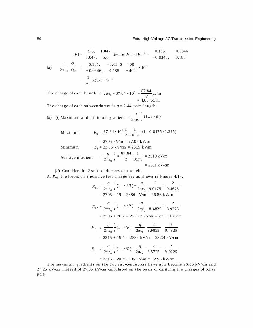
80 Extra High Voltage AC Transmission Engineering
[P] =
−
−==
−
185.0,0346.0
0346.0,185.0][][giving
6.5,047.1
047.1,6.5 1PM
(a)
π 2
1
021
e = 310400
400
185.0,0346.0
0346.0,185.0×
−
−
−
= 31084.871
1×
−
The charge of each bundle is c/m18
84.871084.872 3
0 µ=××πe
= 4.88 µc/m.The charge of each sub-conductor is q = 2.44 µc/m length.
(b) (i) Maximum and minimum gradient = )/1(1
2 0
Rrre
q±
π
Maximum E0 = )225.0/0175.01(0175.01
21
1084.87 3 +×
= 2705 kV/m = 27.05 kV/cm Minimum Ei = 23.15 kV/cm = 2315 kV/m
Average gradient = kV/m25100175.
1284.871
2 0
==π req
= 25.1 kV/cm(ii) Consider the 2 sub-conductors on the left.
At P01, the forces on a positive test charge are as shown in Figure 4.17.
E01 =
+
π−+
π 4675.92
0175.92
2)/1(
12 00 e
qRr
req
= 2705 – 19 = 2686 kV/m = 26.86 kV/cm
E02 =
+
π++
π 9325.82
4825.82
2)/1(
12 00 e
qRr
req
= 2705 + 20.2 = 2725.2 kV/m = 27.25 kV/cm
1iE =
+
π+−
π 4325.92
9825.82
2)/1(
12 00 e
qRr
req
= 2315 + 19.1 = 2334 kV/m = 23.34 kV/cm
2iE =
+
π−−
π 0225.92
5725.82
2)/1(
12 00 e
qRr
req
= 2315 – 20 = 2295 kV/m = 22.95 kV/cm.The maximum gradients on the two sub-conductors have now become 26.86 kV/cm and
27.25 kV/cm instead of 27.05 kV/cm calculated on the basis of omitting the charges of otherpole.

Voltage Gradients of Conductors 81
(c) The average maximum gradient is defined as the arithmetic average of the twomaximum gradients.
Eavm = kV/cm055.27)25.2786.26(21
=+
This is almost equal to the maximum gradient obtained by omitting the charges of theother pole.
For a 3-phase ac line, the effect of charges on other phases can usually be ignored becausewhen the charge on the conductor of one phase is at peak value, the charge on the other phasesare passing through 50% of their peak values but of opposite polarity. This has an even lesseffect than that has been shown for the bipolar dc line where the charge of the second pole isequal and opposite to the charge of the conductor under consideration. However, in a digitalcomputer programme, all these could be incorporated. It is well to remember that all calculationsare based on the basic assumption that ground is an equipotential surface and that the sub-conductor charges are concentrated at their centres. Both these assumptions are approximate.But a more rigorous analysis is not attempted here.
4.5.3 Maximum Surface Voltage Gradients for 3N ≥The method described before for calculating voltage gradients for a twin-bundle conductor, N =2, can now be extended for bundles with more than 2 sub-conductors. A general formula will beobtained under the assumption that the surface voltage gradients are only due to the chargesof the N sub-conductors of the bundle, ignoring the charges of other phases or poles and thoseon the image conductors. Also, the sub-conductors are taken to be spaced far enough from eachother so as to yield a uniform field at the location of the sub-conductor and hence the concept ofstress-doubling will be used.
Figure 4.18 shows bundles with N = 3, 4, 6, 8 sub-conductors and the point P where themaximum surface voltage gradient occurs. The forces exerted on a unit positive test charge atP due to all N conductor-charges q are also shown as vectors. The components of these forcesalong the vector force due to conductor charge will yield the maximum surface voltage gradient.Due to symmetry, the components at right angles to this force will cancel each other, as shownon the figures.
N = 3. B = R3 for equilateral spacing.
Fig. 4.18 Distribution of surface voltage gradients on 3-, 4-, 6-, and 8-conductor bundles.
B
B
R
P30°
qe2 0π
qe2 0π
qe2 0π
2/ 3
R
R
P45° 30° 60°
R
B
R
B
2 sin /8R π
2 sin /4R π
2 s in3R π/8
( )a ( )b( )c
( )d
R = B/ 3 R = B/ 2 R = B R = B/2 sin 22.5°
qe2 0π
2B
. qe2 0π
2B
.qe2 0π
2B
.qe2 0π
1r
.qe2 0π
1r
.qe2 0π
1r
. 2R2
.2R2
.
.

82 Extra High Voltage AC Transmission Engineering
EP = )/21(1
230cos
2.21
12 00
Rrre
qB
rre
q+
π=
°×+
π ...(4.53)
The sub-conductor charge is q = Q/3 where Q is obtained from equation (4.32),]][[]2/[ 0 VMeQ =π as discussed earlier.
N = 4.B = R2 for quadrilateral spacing.
EP =
°×++
π45cos
2
22
221
2 0 RRreq
= )/31(1
2 0
Rrre
q+
π ...(4.54)
Note the emergence of a general formula
EP = ]/)1(1[1
2 0
RrNre
q−+
π ...(4.55)
N = 6. B = R for hexagonal spacing.
EP =
°×+°×++
π30cos
3
2260cos
22
221
2 0 RRRreq
= ]/)1(1[1
2)/51(
12 00
RrNre
qRr
req
−+π
=+π ...(4.56)
N = 8, B = 2R sin 22°.5 for octagonal spacing
EP = +
π×
π×+
ππ
×++π 4
cos4/sin2
22
83
cos8/sin2
22
221
2 0 RRRreq
π
π 8cos
8/3sin22
2R
= )/71(1
222211
2 00
Rrre
qRRRRre
q+
π=
++++
π
= ]/)1(1[1
2 0
RrNre
q−+
π ...(4.57)
From the above analysis, we observe that the contributions to the gradient at P from each
of the (N – 1) sub-conductors are all equal to Req 1
2 0π . In general, for an N-conductor bundle,
EP =
π
×+
π−ππ
×++π NRNNRRreq
/2sin22
22
cos/sin2
22
221
2 0
π−−ππ−
×++
π−πN
NNNRN
12
cos/)1sin(2
22...
22
cos
= ]/)1(1[1
2)2(11
2 00
RrNre
qR
NRre
q−+
π=
−
++π ...(4.58)
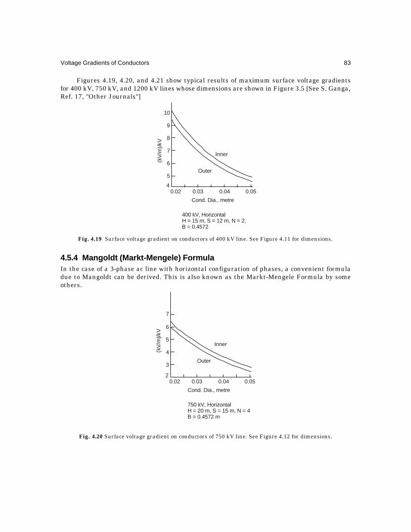
Voltage Gradients of Conductors 83
Figures 4.19, 4.20, and 4.21 show typical results of maximum surface voltage gradientsfor 400 kV, 750 kV, and 1200 kV lines whose dimensions are shown in Figure 3.5 [See S. Ganga,Ref. 17, "Other Journals"]
Fig. 4.19 Surface voltage gradient on conductors of 400 kV line. See Figure 4.11 for dimensions.
4.5.4 Mangoldt (Markt-Mengele) FormulaIn the case of a 3-phase ac line with horizontal configuration of phases, a convenient formuladue to Mangoldt can be derived. This is also known as the Markt-Mengele Formula by someothers.
Fig. 4.20 Surface voltage gradient on conductors of 750 kV line. See Figure 4.12 for dimensions.
10
9
8
7
6
5
40.02 0.03 0.04 0.05
Inner
Outer
(kV
/m)/k
V
Cond. Dia., metre
400 kV, HorizontalH = 15 m, S = 12 m, N = 2,B = 0.4572
7
6
5
4
3
20.02 0.03 0.04 0.05
Inner
Outer
(kV
/m)/k
V
Cond. Dia., metre
750 kV, HorizontalH = 20 m, S = 15 m, N = 4B = 0.4572 m

84 Extra High Voltage AC Transmission Engineering
Fig. 4.21 Surface voltage gradients on 1200 kV lines. See Figure 4.13 for dimensions.
Referring to Figure 4.22, let Q1, Q2, Q3 be the instantaneous charges on the bundles. TheMaxwell's Potential coefficients are
+=+==
+=+====
====
2223113
22232232112
/1332211
)/(1ln)2/44ln(
)/2(1ln)/4ln(
)/(where),/2ln(
SHSSHPP
SHSSHPPPP
RNrRrrHPPP Neqeq
...(4.59)
Fig. 4.22 3-phase horizontal configuration of line for derivation of Mangoldt Formula.
5
4
3
2
10.02 0.03 0.04 0.05
(kV
/m)/k
V
Cond. Dia., metre
1200-kV HorizontalH = 20, S = 24, N = 8, R = 0.6
4 + 4H S22
4 + H S22
Q1Q2 Q3
2HH
S
2S
S
R2r
N -
r
conductor bundleeq N= R Nr/R ( )1/

Voltage Gradients of Conductors 85
The voltage-charge relations are
π+π+π=
π+π+π=
π+π+π=
0333023201313
0323022201212
0313021201111
2/.2/.2/.
2/.2/.2/.
2/.2/.2/.
eQPeQPeQPV
eQPeQPeQPV
eQPeQPeQPV
...(4.60)
Both the voltages and the charges are sinusoidally varying at power frequency and at
every instant of time, 0321 =++ VVV and 0321 =++ QQQ . When the charge of any phase is
passing through its peak value, the charges of the remaining two phases are negative but ofmagnitude 0.5 peak. From symmetry, the peak values of charges on the two outer phases willbe equal. If we assume the peak values of Q1, Q2, Q3 to be approximately equal, then, combiningequations (4.59) and (4.60) we obtain the following equations:
For the Outer Phases
V1 = )5.05.0(2 131211
0
1 PPPe
Q−−
π
=4/1
220
1
12
1
12ln
2
+
+
π
SH
SH
rH
eQ
eq
...(4.61)
Therefore, 0
1
2 eQπ
is found from the given voltage. If the r.m.s. value of phase voltage to
ground is used, 0
1
2 eQπ
is also the r.m.s. value of the charge coefficient and the resulting surface
voltage gradient will also be in kV (r.m.s.)/metre, if V is in kV. The maximum surface voltagegradient will then be according to equation (4.58).
E0m =
−+
π Rr
NrNe
Q)1(1
112 0
1
= ,
])/(1)/2(1[
12ln..
/)1(1
4/122
V
SHSHrHrN
RrN
eq ++
−+...(4.62)
Similarly, for the centre phase,
0
2
2 eQπ = VPPP .)](5.0[ 1
232122−+−
and Ecm = V
SHrHrN
RrN
eq2/12 ])/2(1[
12ln.
/)1(1
+
−+...(4.63)

86 Extra High Voltage AC Transmission Engineering
Equations (4.62) and (4.63) are known as Mangoldt or Markt-Mengele Formulas. Theywere first derived only for the centre phase which gives a higher maximum voltage gradientthan the outer phases. With corona assuming lot more importance since this formula wasderived, we have extended their thinking to the outer phases also.
Example 4.10. For a 400-kV line, calculate the maximum surface voltage gradients onthe centre and outer phases in horizontal configuration at the maximum operating voltage of420 kV, r.m.s. line-to-line. The other dimensions are
H = 13 m, S = 11 m, N = 2, r = 0.0159 m, B = 0.45 m.Solution. 2H/S = 26/11 = 2.364 and H/S = 1.182
4/122 ])/(1)/2(1[ SHSH ++ = 567.2)/(1;982.1 2 =+ SH
eqr = R(N .r/R)1/N = 0.225 (2 × 0.0159/0.225)1/2 = 0.0846 m
Also, req = 3.307/2,m0846.045.00159.0 ==× eqrH
(a) Outer Phases
E0m =)982.1/3.307(ln0159.02
3/420)225.0/0159.01(×+
= 1619 kV/m = 16.19 kV/cm
(b) Centre Phase.
Ecm =)567.2/3.307ln(0159.02
3/420)225.0/0159.01(×+
= 1707 kV/m = 17.07 kV/cm
The centre phase gradient is higher than that on the outer phases by
10019.16
19.1607.17 ×− = 5.44%
For a bipolar dc line, it is easy to show that the maximum surface voltage gradient on thesub-conductor of a bundle is
Em = V
PHrHrN
RrN
eq
+
−+
2)/2(1
12ln..
/)1(1...(4.64)
where H = height of each pole above groundP = pole spacing
and V = voltage to ground
Example 4.11. Using the data of Example 4.9, and using equation (4.64), calculate themaximum surface voltage gradient on the 2-conductor bundle for ± 400 kV dc line.
Solution. H = 12, P = 9, r = 0.0175, N = 2, R = 0.225req = 0.08874,

Voltage Gradients of Conductors 87
Em =
+×
+
2)9/24(1
108874.
24ln0175.02
400)225.0/0175.01(
= 2705 kV/m = 27.05 kV/cm
4.6 EXAMPLES OF CONDUCTORS AND MAXIMUM GRADIENTS ONACTUAL LINES
Several examples of conductor configurations used on transmission lines following world-widepractice are given in the Table 4.1. The maximum surface voltage gradients are also indicated.These are only examples and the reader should consult the vast literature (CIGRE Proceedings,etc.) for more details. Most conductor manufacturers use British units for conductor sizes andthe SI units are given only for calculation purposes. These details are gathered from a largenumber of sources listed in the bibliography at the end of the book.
The conductor sizes given in the table are not the only ones used. For example, thefollowing range of conductor sizes is found on the North American continent.
345 kV. Single conductor— 1.424, 1.602, 1.737, 1.75, 1.762 inches dia
2-conductor bundle—1.108, 1.165, 1.196, 1.246 inches dia.500 kV. Single conductor — 2.5 inches dia
2-bundle—1.602, 1.7, 1.75, 1.762, 1.82 inches dia (ACAR).
3-bundle—1.165 inches dia.
4-bundle—0.85, 0.9, 0.93 inches dia.
735-765 kV 4-bundle—1.165, 1.2, 1.382 inches dia.
4.7 GRADIENT FACTORS AND THEIR USEFrom the Mangoldt (Markt-Mengele) formula given in Section 4.5, it is observed that themaximum surface voltage gradient in the centre phase of a horizontal 3-phase ac line is afunction of the geometrical dimensions and the maximum operating voltage V. As shown inTable 4.1, the maximum operating voltages show a wide variation. It is therefore advantageousto have a table or graph of the normalized value called the 'gradient factor' in kV/cm per kV orV/m per volt or other units which will be independent of the voltage. The gradient factor isdenoted by gf = Ecm/V and its value is
gf = Ecm/V =
+
−+
2)/2(1
12ln..
/)1(1
SHrHrN
RrN
eq
...(4.65)

88 Extra High Voltage AC Transmission Engineering
Table 4.1. Conductor Details and Maximum Surface Voltage Gradients Used in EHV Lines
Country Maximum Conductor Details Maximum GradientOperating Voltage No. × dia in inches (cm) kv/cm, RMS
kV, RMS
(1) India 420 2 × 1.258 (3.18) 17.0(2) Canada 315 2 × 1.382 (3.51) 17.4
380 2 × 1.108 (2.814) 17.5 – 18.0525 4 × 0.93 (2.362) 18.8735 4 × 1.2, 1.382 (3.05, 3.51) 17.7–20.4
1200 6 × 1.84, 2.0 (4.674, 5.08) –8 × 1.65, 1.84 (4.19, 4.674) –
(3) U.S.A. 355 – 362 1 × 1.602 (4.07) 16.62 × 1.175, 1.196 (2.985, 3.04) 15–16
500 2 × 1.65 (4.19) 16.93 × 1.19 (3.02) 16.4
550 2 × 1.6 (4.07) 16.91 × 2.5 (6.35) 16.7
765 4 × 1.165 (2.96) 20.41200 8 × 1.602 (4.07) 13.5
(4) U.S.S.R. 400 3 × 1.19 (3.02) 13.6525 3 × 1.19 (3.02) 18.0
1200 8 × 0.96 (2.438) 21.4(5) U.K. 420 2 × 1.09 (2.77) 19.6
4 × 1.09 (2.77) 13.5(6) France 420 2 × 1.04 (2.64) 19.0(7) Germany 380 4 × 0.827 (2.1) 15.7
420 4 × 0.854 (2.17) 16.7(8) Italy 380 2 × 1.168 (2.97) 15.0
1050 4 × 1.76, 1.87 (4.47, 4.75) 17.1 – 19.86 × 1.5 (3.81) –
(9) Sweden 380 3 × 1.25 (3.18) 12.5400 2 × 1.25 (3.18) 16.5800 4 × 1.6 (4.06) 17.6
By varying the parameters (r, N, R, H and S) over a large range curves can be plotted forgf against the desired variable. From product of gf and the maximum operating line-to-groundvoltage of the line, the maximum surface voltage gradient is readily obtained. Such curves areshown in Figure 4.23 for N = 1, 2, 4 and for conductor diameters ranging from 0.7" to 2.5" (1.78cm to 6.35 cm). The height H in all cases has been fixed at H = 50' (15 m) and the phase spacingS ranging from 20' to 50' (6 to 15 m). Calculations have shown that a variation of height H from10 to 30 m etres does not change gf by more than 1%. The abscissa has been chosen as the

Voltage Gradients of Conductors 89
reciprocal of the diameter and the resulting variation of gradient factor with (1/d) is nearly astraight line, which is very convenient. In equation (4.65) it is observed that the conductorradius occurs in the denominator and this property has been used in plotting Figure 4.23. [Alsosee G. Veena, Ref. 16, "Other Journals"].
Fig. 4.23 Gradient factors of conductors (gf in V/m/Volt).
Such graphs can also be prepared for the maximum surface voltage gradient factors forthe outer phases or bipolar dc lines, etc., in a design office.
4.8 DISTRIBUTION OF VOLTAGE GRADIENT ON SUB-CONDUCTORSOF BUNDLE
While discussing the variation of surface voltage gradient on a 2-conductor bundle in section4.5.2, it was pointed out that the gradient distribution follows nearly a cosine law, equation(4.52). We will derive rigorous expressions for the gradient distribution and discuss theapproximations to be made which yields the cosine law. The cosine law has been verified tohold for bundled conductors with up to 8 sub-conductors. Only the guiding principles will beindicated here through an example of a 2-conductor bundle and a general outline for N ≥ 3 willbe given which can be incorporated in a digital-computer programme.
Figure 4.24 shows detailed view of a 2-conductor bundle where the charges q on the twosub-conductors are assumed to be concentrated at the conductor centres. At a point P on thesurface of a conductor at angle θ from the reference direction, the field intensities due to thetwo conductor charges are, using stress-doubling effect,
E1 = B'eq
Ere
q 22
and1
2 02
0 π=
π ...(4.66)
16
14
12
10
8
6
4
2
00.20 0.25 0.30 0.35 0.40 0.45
S
61215
6 915
915
N = 2
N = 4
N = 1
Gradient Factors(k
V/m
)/kV
1/d, d in cm


Voltage Gradients of Conductors 91
Fig. 4.25 Six-conductor bundle and gradient on sub-conductor.
We first evaluate the distances '' BB 1612 to .
'B12 = ])cos60cos()sin60sin[( 22 θ+°+θ+° rRrR
'B13 = ])cos30cos3()sin30sin3[( 22 θ+°+θ+° rRrR'B14 = ])cos2()sin[( 22 θ++θ rRr ...(4.72)
'B15 = ])cos30cos3()sin30sin3[( 22 θ+°+θ−° rRrR'B16 = ])cos60cos()sin60sin[( 22 θ+°+θ−° rRrR
Next the horizontal and vertical components of the field intensity at P are evaluated. Thefactor )2/( 0eq π is omitted in writing for the present but will be included at the end.
Conductor i Horizontal component Vertical component(i = 1, 2, 3 Eh(i) Ev(i)
4, 5, 6)
1. θcos1r
θsin1r
2. 212 )/()cos60cos(2 'BrR θ+° 2
12 )/()sin60sin(2 'BrR θ+°
3. 213 )/()cos30cos3(2 'BrR θ+° 2
13 )/()sin30sin3(2 'BrR θ+°
4. 214 )/()cos2(2 'BrR θ+ 2
14 )/(sin2 'Br θ
5. 215 )/()cos30cos3(2 'BrR θ+° 2
15 )/()sin30sin3(2 'BrR θ−°−
6. 216 )/()cos60cos(2 'BrR θ+° 2
16 )/()sin60sin(2 'BrR θ−°−
Total field intensity
EP(θ) =
2/126
1
26
10
)()(2
+
π ∑∑== i
vi
h iEiEe
q
Figure 4.26 shows examples of surface voltage gradient distributions on bundled conductorswith N = 2, 4, 6 subconductors.
1
2
P θ
B'15
B'14
B'13 B'12
B'16
3
4
5 6

92 Extra High Voltage AC Transmission Engineering
Fig. 4.26 Distribution of voltage gradient on bundle conductors for N = 2, 4, 6.Variation with conductor diameter.
4.9 DESIGN OF CYLINDRICAL CAGES FOR CORONA EXPERIMENTSThe effects of high voltage-gradients on bundled conductors are evaluated all over the world by"cages". In the simplest of these arrangements a large metallic cylinder at ground or nearground potential forms the outer cage with the bundled conductor strung inside. The centres ofthe cylinder and the bundle are coincident while the subconductors themselves are displacedoff-centre, except for N = 1, a single conductor. Several examples are shown in Figure 4.27, inwhich a square cage is also included. When the dimensions of the outer cage become very largeor where the length of conductor and weight are large with a resulting sag, a square cage madewith mesh can be contoured to follow the sag. The cage arrangement requires lower voltage forcreating the required surface voltage gradient on the conductors than in an overhead lineabove ground. Also artificial rain equipment can be used if necessary to obtain quick results.Measuring instruments are connected to ground both from the conductor at high voltage andthe cage at near ground potential where necessary for Radio Interference, Corona Loss, charge,etc., measurements. Audible noise is usually measured as radiation into a microphone placedaway from the test setup. Normally, the cage consists of three sections, a long middle sectionwhich is the principal cage which could extend up to 60 metres, with two short guard cages ateither end grounded in order to minimize edge effects.
Fig. 4.27 Configuration of 'cages' used for corona studies.
1.2
1.1
1.0
0.9
0.8
0.7
180° 360°
N = 6
1.3 1.3
1.2 1.2
1.1 1.1
1.0 1.0
0.9 0.9
0.8 0.8
0.7 0.7
0.03
0.02
360° 360°180°
0.05
N = 2 N = 4
Cond. Dia., metre
2R
RC
2r

Voltage Gradients of Conductors 93
We will derive equations for calculating corona-inception gradient on given bundledconductors when placed inside a cylindrical outer cage of a given radius. Before this is carriedout, the results of such calculations are presented for bundles up to 8 sub-conductors which adesigner can use. Figures 4.28 (a), (b), (c) give the variation of r.m.s. value of corona-inceptionvoltage which will be required from the single-phase transformer that excites the entireexperiment. The diameters of the sub-conductors in 2, 4, 6 and 8 conductor bundles have beenvaried from 0.02 to 0.055 metre (0.8 to 2.2 inches), and the outer radius of the cylinder from 2to 5 metres, (4 to 10m diameters). For 2- and 4-conductor bundles, the bundle spacing B istaken to be 18 inches (45.72 cm) while for the 6-, and 8-conductor bundles the bundle radius Rhas been fixed at 0.6 m (1.2 m diameter). The voltages shown are for smooth conductors. On arough stranded conductor the corona-inception occurs at a lower voltage and a suggestedroughness factor is 1.4. Thus, the ordinates must be divided by this factor to yield the requiredcorona-inception voltage in practical cases.
Fig. 4.28 Corona-inception voltage on bundled conductors inside cylindrical cage of radius Rc.Smooth-conductor values.
(a) 2-and 4-conductor bundles.(b) 6-conductor bundle.(c) 8-conductor bundle.
4.9.1 Single Conductor Concentric with CylinderFigure 4.29 shows a coaxial cylindrical cage with outer cylinder radius Rc and inner conductorradius r. The problem is the same as a coaxial cable with air dielectric. At any radius x, the fieldstrength is
Ex = xeq 1
2 0π and the voltage is ∫ π
=π
=cR
r
c
rR
eq
xdxe
qV ln
2/
2 00
1000
1200
1000
800
1000
800
600
800
600
400
600
400
200
400
200200
0 00
N = 4
N = 2
kV
5
5
5
4
4
4
3
3
3
3
2
2
2
Rc
Rc
Rc
N = 2 and 4 N = 8N = 6
0.02 0.020.020.04 0.040.040.06 0.060.06Conductor Dia., metre Conductor Dia., metreConductor Dia., metre
( )a ( )b ( )c
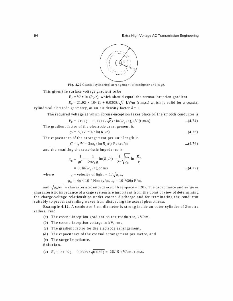
94 Extra High Voltage AC Transmission Engineering
Fig. 4.29 Coaxial cylindrical arrangement of conductor and cage.
This gives the surface voltage gradient to beEr = V/r ln (Rc/r), which should equal the corona-inception gradient
E0 = 21.92 × 10² (1 + 0.0308/ r kV/m (r.m.s.) which is valid for a coaxialcylindrical electrode geometry, at an air density factor δ = 1.
∴ The required voltage at which corona-inception takes place on the smooth conductor is
V0 = ),/ln()./0308.01(2192 rRrr c+ kV (r.m.s) ...(4.74)
The gradient factor of the electrode arrangement isgf = )/ln(/1/ rRrVE cr = ...(4.75)
The capacitance of the arrangement per unit length is
C = )/ln(/2/ 0 rReVq cπ= Farad/m ...(4.76)
and the resulting characteristic impedance is
Z0 =
µπ
=π
=r
Re
rRgegC
cc ln
21
)/ln(2
11
0
0
0
= ohms),/ln(60 rRc ...(4.77)
where g = velocity of light = 00/1 eµ
0µ = 4π × 10–7 Henry/m, e0 = 10–9/36π F/m,
and 00/eµ = characteristic impedance of free space = 120π. The capacitance and surge orcharacteristic impedance of a cage system are important from the point of view of determiningthe charge-voltage relationships under corona discharge and for terminating the conductorsuitably to prevent standing waves from disturbing the actual phenomena.
Example 4.12. A conductor 5 cm diameter is strung inside an outer cylinder of 2 metreradius. Find
(a) The corona-inception gradient on the conductor, kV/cm,
(b) The corona-inception voltage in kV, rms,
(c) The gradient factor for the electrode arrangement,
(d) The capacitance of the coaxial arrangement per metre, and
(e) The surge impedance.Solution.
(a) E0 = =+ )025.0/0308.01(92.21 26.19 kV/cm, r.m.s.
x
dx

Voltage Gradients of Conductors 95
(b) V0 = E0r ln (Rc/r) = 26.19 × 2.5 ln (200/2.5) = 26.19 × 10.955 kV
= 286.9 kV, r.m.s.(c) The gradient factor is 26.19/286.9 = 0.0913 kV/cm per kV
Also, 1/r ln (Rc/r) = 0.0913. or V/cm per V
(d) C = F/m68.12)80ln(18
10)/ln(
29
0 µµ=×
=π −
rRe
c
(e) Z0 = 60 ln (Rc/r) = 263 ohms
Also, Z0 = 1/gC = 1/(3 × 108 × 12.68 × 10–12) = 263 ohms.Such an arrangement with a single conductor is not of much use in extra high voltage
investigations since the conductor is invariably a bundled conductor without exception. However,when the cage consists of shapes other than cylinders, or in a large hall of a high voltagelaboratory, it is very important to have an idea of the gradient factor and an equivalent radiusof the cage or hall. This is determined experimentally by stringing a smooth aluminium orcopper tube of known diameter for which corona-inception gradient is known. A radio noisemeter is used to determine the corona inception and the voltage initiating the reading on themeter is accurately determined. This yields the gradient factor from which the equivalentradius Rc of the outer electrode can be easily calculated. The smooth tube must be preferablystrung at the centre of the hall or where normal RIV (Radius Influence Voltage) measurementsare carried out. In a square cage, the smooth tube is accurately centred. The equivalent radiuscan be used for measurements and interpretation of results obtained with bundled conductors.This will form the contents of further discussion.
4.9.2 Bundled Conductors Inside a CylinderWhen a bundle with N sub-conductors is centred inside a cylinder, the conductors themselvesare eccentric with respect to the cylinder. We now examine the properties of the electric fieldwhen a conducting cylinder is placed off-centre inside a larger conducting cylinder. This problemparallels the sphere-gap problem discussed earlier.
4.9.2.1 Single Conductor with Eccentricity
Figure 4.30 shows a cylinder of radius Rc in which is located a conductor of radius rc withits centre displaced by a distance R from the centre of the outer cylinder. Both the cylindricalelectrodes are equipotentials with voltage V applied between them. In nearly all cases, theouter cylinder is grounded and its potential is zero. The two circles (in two dimensions) of radiirc and Rc can be made equipotential lines under the influence of two equal but opposite charges+q and –q per unit length which are located as shown in Figure 4.30. An important property ofthe field, which will be proved later in order not to interrupt continuity at this stage and whichwill be used for cage designs, is
radiuscylinder the of square
cylinder given a of centre
thefrom charges two the
to distances of Product
=
...(4.78)

96 Extra High Voltage AC Transmission Engineering
Fig. 4.30 Outer cylinder with eccentric conductor.
=−
=+2
12
221
)(and
)(Thus,
c
c
rRRR
RRRR...(4.79)
Since we are given rc, Rc, and R, the radii and the eccentricity, it is easy to determine R1and R2 as follows:
Let D = RrRR cc /)( 222 −+ . Then
R1 = RRRDD cc /)(5.0 222 ≈−+ when 22 RRc + ,2cr
and R2 = )/( 12 RRrc − .
The voltage required in terms of the charge q is
V =210
21
0
ln2
))((ln
2 RRrR
eq
rRRRRR
eq cc
cc π=
+−π ...(4.80)
This will also be derived later. The maximum surface voltage gradient on the innerconductor is ),2/( 0 creq π if we assume the other charge to be located very far. For corona-inception, this gradient should equal the corona-inception gradient
E0 = kV/m)/0308.01(2192 cr+
∴ V0 =21
ln.)./0308.01(2192RRrR
rr cccc+ ...(4.81)
Note that when the inner conductor is concentric with the cylinder, R = 0 and R1 R2 = 2cR .
This reduces to equation (4.74) derived before.All quantities in equation (4.81) are known so that the corona-inception voltage for a
smooth conductor can be determined. The capacitance of the eccentric conductor and cylinderis obviously
C =
π=
210 ln/2/
RRrReVq cc , Farad/meter ...(4.82)
The surge impedance is
Z0 =21
8 ln60103/1RRrR
C cc=× ...(4.83)
rc
Rc
R1
– q
+ q
R2
R

Voltage Gradients of Conductors 97
The above analysis becomes very cumbersome when there are more than one eccentricconductor. We will develop a very general method in the next section based on the ideasdeveloped here for one eccentric conductor.
Example 4.13. A stranded conductor 3.5 cm diameter (rc = 0.0175 m) is displaced by R =22.5 cm from the centre of a cylinder 3.2 metres is diameter (Rc = 1.6 m). Taking a roughnessfactor m = 1.4, calculate
(a) the charge coefficient 02/ eq π at corona inception,(b) the location of charges q and – q,(c) the corona-inception voltage V0, and(d) the capacitance per metre and surge impedance based on light velocity.Solution. Because of surface roughess, corona-inception takes place at a gradient equal
to (1/1.4) times that on a smooth conductor.
Eor = )0175.0/0308.01(4.192.21
+ = 19.3 kV/cm = 1930 kV/m
(a) 02/ eq π = rc. Eor = 33.81 kV
(b) D = RrRR cc /)( 222 −+ = (1602 + 22.52 – 1.752)/22.5 = 1161 cm
R1 = )(5.0 22cRDD −+ = 1155 cm = 11.55 m
R2 = )/( 12 RRrc − = 2.7 × 10⁻³ cm = 2.7 × 10⁻⁵ m
Note that the negative charge is displaced from the centre of the inner conductor by only2.7 × 10–3 cm while the positive charge is located very far (11.55 m) from the centre of the outercylinder.
(c) Corona-inception voltageV0 = 19.32 × 1.75 ln [(1155 – 22.5) 22.5/(160 × 1.75)]
= 33.81 ln 91 = 33.81 × 4.51 = 152.5 kV.
(d) Capacitance C = F/m316.1291ln/18
109
µµ=−
Surge impedance Z0 = 1/Cg = 1012/12.316 × 3 × 108 = 271 ohms.
Example 4.14. Repeat the previous problem if the inner conductor is concentric with theouter cylinder.
Solution. (a) 02/ eq π = 0,(b)kV;81.33 21 =∞= RR
(b) V0 = kV6.152)/ln(. =ccorc rREr
(c) C = F/m3.12)/ln(/2 0 µµ=π cc rRe
Z0 = 1012/12.3 × 3 × 108 = 271 ohms.The displacement of the conductor by 22.5 cm in a cylinder of radius 160 cm, i.e., 14%
eccentricity has not made a noticeable difference in the corona-inception voltage, etc., for thedimensions given. (This is one conductor of a 2-conductor bundle with 45 cm bundle spacingplaced inside a cylinder 10 ft in diameter).
We now give a proof for equations (4.78) and (4.79), which are also given in any standardtext book on electrostatics (see Bewley or Zahn, under "Books" in Bibliography). Figure 4.31

98 Extra High Voltage AC Transmission Engineering
shows two line charges + q and – q coulomb/metre separated by a distance 2S. At a pointmidway between them the potential is zero and we can choose this as the origin of a coordinatesystem. The potential of a point P(x, y) with respect to the reference point 0 will be, accordingto equation (3.35)
V = 22
22
00 )(
)(ln
4charge positivefrom Distancecharge negativefrom Distance
ln2 ySx
ySxe
qe
q
++
+−π
=π ...(4.84)
Fig. 4.31 Location of charges and an equipotential surface of radius Rc with potential Vc
If we denote U = exp ( )/4 0 qVeπ , a constant-potential line in the field of the two charges
will satisfy the equation(x – S)2 + y2 = U[(x + S)2 + y2]
or2
2
11
yUU
Sx +
−+
− = 4S2 U/(1 – U)2 ...(4.85)
This is a circle with radius )1/(2| UUS −=ρ | and centre at
−+
0,11
UU
S on the line
joining the two charges.A circle of radius Rc has the potential given by
2cR =
cc
ccc U
SU
SUUUS
−−=−
12
12
)1/(4 22 ...(4.86)
Now, referring to Figure 4.31 and equation (4.86), we observe that the distances of thetwo charges from the centre of the circle (a cylinder in 3 dimensions) are
1ρ = ,1
211
and,12
11
2cc
c
c
c
c
c
US
SUU
SU
SUS
UU
S−
=+−+
=ρ−
=−−+
Their product is 2
2
21)1(
4
c
c
UUS
−=ρρ which is 2
cR according to equation (4.86). Therefore
equation (4.78) result.In order to derive equation (4.80), refer to Figure 4.30, and consider the line joining the
two charges and the points where it intersects the two cylinders of radii Rc and rc. The potentialsof these two points, resulting from equation (3.35), are as follows:
P x, y( )
S S
– q+ q
ρ = 2S U/1 – U( )
Vc
11 + U – US R = 2S U /1 – Uc c c( )
Uc = e4πe V / q0 c

Voltage Gradients of Conductors 99
On the inner conductor:
Vi = )]/()ln[()2/( 120 cc rRRRreq −−−π ...(4.87)On the outer cylinder:
V0 = )]/()ln[()2/( 120 cc RRRRReq −−−π ...(4.88)Now, from equation (4.79),
R2 + R = 22
12 /and,/ RrRRRR c1c =− .
∴ Vi =ccc
c
rR
eq
rRrRr
eq 2
022
2
0ln
2/ln
2 π=
−−
π ...(4.89a)
V0 =101
12
0ln
2/
ln2 R
Re
qRR
RRRe
q c
c
cc
π=
−−
π ...(4.89b)
∴ The p.d. between the inner conductor and outer cylinder is
V =210
0 ln2 RR
rRe
qVV cc
i π=− ...(4.90)
4.9.2.2 Multi-conductors with Eccentricity Inside Cylinder
The corona-inception voltage of a single conductor of radius rc placed off-centre inside acylinder of radius Rc was derived before, Figure 4.30. In order to handle more conductors, wegive a different method. This uses a circle called the "Circle of Inversion" whose radius is 2Rcand touches the cylinder at one point.
Consider Figure 4.32 in which is shown a circle of radius Rc with centre at O, and anotherwith radius 2Rc and centre O' with both circles touching at O". A straight line FF is drawnthrough O" tangent to both circles. Taking a point P on circle Rc, extend O' to P to cut FF in P'.Then
O'P × O'P' = (2Rc)2 = 24 cR ...(4.90)
which is proved as follows: Let φ=∠O"O'P . Then
O'PO"∠ = φ=φ=°=∠ cos/2,cos2,90 cc RO'P'RO'PO'O"P'
giving O'P'O'P × = 24 cR . All points inside circle Rc fall above FF.
Fig. 4.32 Circle of inversion and outer cylinder of cage arrangement.
This is true of all points such as P on the circle of radius Rc. Thus, the straight line FF isthe locus of all points on the circle Rc about the circle of inversion with radius 2Rc and centre at
φRc
2Rc
90°
F
P
F
O
O'
O" P'

100 Extra High Voltage AC Transmission Engineering
O'. If the circle is the outer cylinder of a "cage" arrangement, then it has been transformed intoa straight line and every point on it is the inverse point on the circle. Any other small cylinderof radius rc placed with an eccentricity R can also be transformed into a cylinder about thecircle of inversion. Then Maxwell's Potential coefficients can be utilized to formulate the chargeequation in terms of the potential of the conductor. This can be done for all the conductors ofthe bundle through matrix [P]. This is carried out as follows: For the point P0, the centre ofconductor, an inverse point 'P0 can be found about the circle of inversion from the relation
),/(4/4 20
20 RRRO'PR'O'P ccc +== Figure 4.33. If the charge of the inner conductor is located
at its centre P0, then the imaged charge about the circle of inversion will be located at 'P0 . Itsdistance from the flat surface FF will be
H = )/()(220 RRRRRR'O'P cccc +−=− ...(4.91)
Since the surface is an equipotential at zero potential, the potential of the conductor isV = )/2ln()2/( 0 'rHeq cπ ...(4.92)
Fig. 4.33 Single eccentric conductor inside outer cylinder and circle of inversion for calculation of images.
where 'rc = radius of the image of rc with centre at 'P0 . This is determined as follows:
Choosing two points on a diameter of rc at distances (R – rc) and (R + rc), their inversepoints are located with respect to O' at distances )/(4 2
ccc rRRR −+ and )/(4 2ccc rRRR ++ .
Therefore,
'rc = )]/(1)/(1[4.21 2
ccccc rRRrRRR ++−−+
O'
P "O
P '0
P "'0
Rc
R + r c
P . q 0
R – r c
rc
FF
H
HR
O
OP"' = R / Rc 2
2
H = 2R ———cR – RR + R
c
c 2
r' = —————c4R r
(R + R) –rc c
c c2

Voltage Gradients of Conductors 101
= ])/[(4. 222cccc rRRRr −+ ...(4.93)
∴ V = RRRR
rRrRR
eq
c
c
cc
cc
+−−+
π
22
0
)(ln
2 ...(4.94)
In practice, Rc + R rc so that
V =cc
c
rRRR
eq 22
0ln
2−
π ...(4.95)
Having located the charge q at 'P0 , the image charge with respect to FF is situated at "P0
at a depth H whose distance from O' is
"O'P0 =RRRR
RRRRR
RHRc
c
c
cccc +
=+
−−=−
4)(222 ...(4.96)
∴ The inverse point of "P0 is located at
'''O'P0 = RRRR"O'PR ccc /)(/4 02 += ...(4.97)
Furthermore, '''OP0 = RRR'''O'P cc /20 =− ...(4.98)
There are now two charges + q and – q located at P0 and "'P0 at the points (O, R) and
)/,( 2 RRO c in whose field the outer cylinder of radius Rc and inner conductor of radius rc areequipotential surfaces. The maximum surface voltage gradient on the surface of the innerconductor is
E = )]/(2/1)[2/( 220 RRRreq cc −+π ...(4.99)
since the distance of "'P0 from the conductor centre is
OP"' – R = RRRc /)( 22 − .
But in terms of potential, equation (4.95), cc
c
rRRR
Ve
q 22
0ln/
2−
=π
The relation between voltage and surface voltage gradient becomes
V = )]/(2/1[ln. 2222
RRRrrRRR
E cccc
c −+
−...(4.100)
For corona-inception to occur, E = )/0308.01(92.21
cor rm
E += , kV/cm, where m =
roughness factor.
Example 4.15. Repeat Example 4.13 using the modified method of images, equation (4.100).Solution. rc = 0.0175 m, Rc = 1.6 m, R = 0.225 m.
Eor = 19.3 kV/cm = 1930 kV/m.
ccc rRRR /)( 22 − = 7.318/1)/(2,90 22 =− RRRr cc
which may be neglected in comparison to 1.

102 Extra High Voltage AC Transmission Engineering
∴ V0 = 1930 × 0.0175 × ln 90 = 152 kVIn Example 4.13, the value obtained was V0 = 152.5 kV.
From this calculation we observe that the effect of image charge located at "P0 is practically
nil on the surface voltage gradient of the conductor (1/318.7 = 0.3%). Hence its presence will beneglected in all further calculations.
N-conductor BundleFor several sub-conductors located off-centre inside the outer cylinder with eccentricity R
from O, we must obtain the location of images of all sub-conductors about the circle of inversionso that Maxwell's Potential Coefficient Matrix will yield the relation between voltage and charge.The computation is lengthy and must be performed step by step. We shall first develop aprogramme suitable for a digital computer commencing with a 2-conductor bundle and extendit to a general case. Figures 4.28 (a), (b), (c) were obtained according to this method and adesigner can use them.
In Figure 4.34, the presence of an image charge is indicated for the 2-conductor bundle,but as mentioned before this can be omitted in all cases. The quantities to be calculated arelisted in a tabular form and will be the sequence of statements in a digital computer programme.
Fig. 4.34 2-conductor bundle inside outer cylinder and its image conductorsabout the circle of inversion.
Quantity Indicated Conductor No. 1 Conductor No. 2
(1) Coordinates of Conductor Xn A1 = – R B1 = R
0Y A2 = O B2 = O
0O'P A3 =22 RRc + B3 = A3
(2) Inverse'O'P0 R1 = 3
2 /4 ARc R2 = R1
φsin S1 = 31/AA S2 = 31/BBφcos S3 = 3/ ARc S4 = 3/BRc
'x0 A4 = R1.S1 B4 = R2.S2
2RB
H
H
F F
2rc2
φ
q
– q
q
– q
Po
P"Rc
2Rc O'
P' x' , y' ( )
O'P"' =4R2cO'P"
o oo
oo
o
o
O

Voltage Gradients of Conductors 103
'y0 A5 = R1S3 – Rc B5 = R2S4 – Rc
(3) Image about FF"x0 A4 B4
"y0 A6 = 52 ARc − B6 = 52 BRc −
"O'P0 R3 =2
624 )( cRAA ++ R4 =
26
24 )( cRBB ++
(4) Inverse of "P0
'''O'P0 A7 = 32/4 RRc B7 = 4
2/4 RRc
'''θsin T1 = 36 /)( RRA c+ T2 = 46 /)( RRB c+
'''θcos T3 = 34 / RA T4 = 44 / RB
'''x0 A8 = 37TA B8 = 47TB
'''y0 A9 = cRTA −17 B9 = cRTB −27
H = cR'y −0 H1 = cRA −5 H2 = H1
'rc G1 = )/(4 223
2ccc rArR − G2 = G1
(5) Potential Coefficients and Charges
P(1, 1) = )/2ln()2,2( 11 GHP = ,
)2,1(P =2
442
55
244
252
)()(
)()2(ln5.0)1,2(
ABABABRABP c
−+−−+−+= ,
V = ).2,1()1,1(,2
)]2,1()1,1([2 00
PPLLe
qPP
eq
+=π
=+π
For unit voltage, 02 e
qπ = 1/L.
(6) Potential GradientDue to positive charge on conductors, the unit gradient is
K1 = )/1/1)(2/( 0 Rreq c +π .
Due to the image charge at '''P0 the gradient is
K2 =
−++−
+−+
−++−
+−π−
218
229
292
182
29
290
)()()()()2/(
ABrAB
rAB
AArAA
rAAeq
c
c
c
c
The total gradient for unit applied voltage, the gradient factor isgf = K1 + 2K2 by taking q/2πe0 = 1/L = 1/[P(1, 1) + P(1, 2)].
The corona-inception gradient is
E0 = kV/m),/0308.01(2192
crm+ .

104 Extra High Voltage AC Transmission Engineering
Then, the corona-inception voltage becomes finally,V0 = E0/gf
Figure 4.28 (a) shows results of corona-inception voltage on a 2-conductor bundle as theinner conductor radius is varied, and for several values of outer-cylinder radius Rc. These arefor smooth conductors for which m = 1.
For 4-, 6-, and 8-conductor bundles, the following steps are used.Computer Programme (for any number of sub-conductors N)
(1) Inputs. Rc = radius of outer cylinder
rc = radius of sub-conductor of bundle
R = bundle radius = eccentricity
N = number of sub-conductors of bundle.
(2) Coordinates of Conductors
IIAy
IAx
−
−
)(:scoordinate
)(:scoordinate
2
1 = 1, 2, ..., N
O'P0 : 22
213 ))(()()( cRIAIAIA −+=
(3) Inverse about the Circle of Inversion
)(: 40 IAO'P' = )(/4 32 IARc
)(:sin 1 ISφ = )(/)( 31 IAIA
)(:cos 2 ISφ = )(/))(( 32 IARIA c+
'x0 : A5(I) = )().( 41 IAIS
'y0 : A5(I) = cRIAIS −)().( 42
H : H(I) = cRIA −)(6
'rc : )(1 IR = ))(/(4 223
2ccc rIArR −
(4) Image of 'P0 about FF
"x0 = 'x0 : A5(I)
"y0 : )(2)( 67 IARIA c −=
"O'P0 : 27
258 ))(()()( cRIAIAIA ++=
(5) Potential Coefficient MatrixSelf coefficient : P(I, I) = ln (2H(I )/R1(I ))
−+−=
−++=≠
211
2
211
2
))()(())()((),(:distance Aerial
))()(())()((),(:distance Image
JAIAJHIHJIF
JAIAJHIHJIBJI
Mutual coefficient : P(I, J) = Ln (B(I, J)/F(I, J))
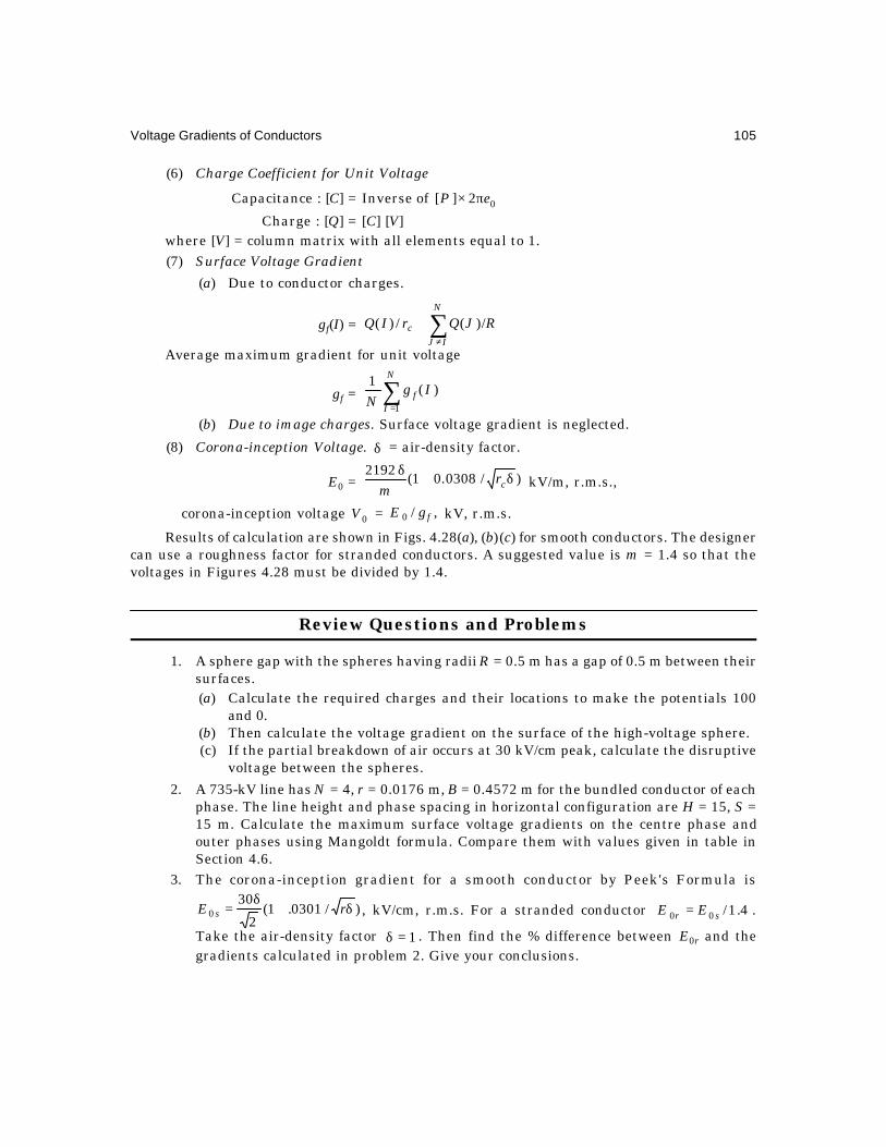
Voltage Gradients of Conductors 105
(6) Charge Coefficient for Unit Voltage
Capacitance : [C] = Inverse of 02][ eP π×
Charge : [Q] = [C] [V]where [V] = column matrix with all elements equal to 1.(7) Surface Voltage Gradient
(a) Due to conductor charges.
gf(I) = ∑≠
+N
IJc RJQrIQ /)(/)(
Average maximum gradient for unit voltage
gf = )(1
1
IgN
N
If∑
=
(b) Due to image charges. Surface voltage gradient is neglected.
(8) Corona-inception Voltage. δ = air-density factor.
E0 = )/0308.01(2192 δ+δ
crm kV/m, r.m.s.,
∴ corona-inception voltage 0V = ,/0 fgE kV, r.m.s.
Results of calculation are shown in Figs. 4.28(a), (b) (c) for smooth conductors. The designercan use a roughness factor for stranded conductors. A suggested value is m = 1.4 so that thevoltages in Figures 4.28 must be divided by 1.4.
Review Questions and Problems
1. A sphere gap with the spheres having radii R = 0.5 m has a gap of 0.5 m between theirsurfaces.(a) Calculate the required charges and their locations to make the potentials 100
and 0.(b) Then calculate the voltage gradient on the surface of the high-voltage sphere.(c) If the partial breakdown of air occurs at 30 kV/cm peak, calculate the disruptive
voltage between the spheres.
2. A 735-kV line has N = 4, r = 0.0176 m, B = 0.4572 m for the bundled conductor of eachphase. The line height and phase spacing in horizontal configuration are H = 15, S =15 m. Calculate the maximum surface voltage gradients on the centre phase andouter phases using Mangoldt formula. Compare them with values given in table inSection 4.6.
3. The corona-inception gradient for a smooth conductor by Peek's Formula is
)/0301.1(2
300 δ+
δ= rE s , kV/cm, r.m.s. For a stranded conductor 4.1/00 sr EE = .
Take the air-density factor 1=δ . Then find the % difference between E0r and thegradients calculated in problem 2. Give your conclusions.

106 Extra High Voltage AC Transmission Engineering
4. A transmission line traverses hills and plains in Northern India. Calculate E0s for a400-kV line with conductor radius r = 0.0159 m for the following sets of elevation inmetres and temperature in °C. (i) 0, 25°, (ii) 1000, 15°, (iii) 2000, 5°, (iv) 3000, 0°C. Useδ = bm(273 + t0)/1013 (273 + t), where bm = barometric pressure in millibars. Assumebm = 1013 at sea level and to drop by 10 millibars for every 100-metre increase inelevation. t0 = 20°C.
Discuss which gives the lowest value for E0s and how a line should be designed forsuch variations.
5. If corona-inception gradient is measured in a h. v. testing laboratory at an elevationof 1000 metres and 25°C, give correction factors to be used when the equipment isused at (a) sea level at 35°C, and (b) 2000 m elevation at 15°C. Use conductor radius= r metre.
6. The outer cylinder of a cage is 2 metres in diameter. A single conductor 4 cm indiameter is strung concentric with it and the arrangement is 30 m long. Calculate(a) the surface voltage gradient (gradient factor) on the conductor, (b) the capacitanceof the arrangement, and (c) the surge impedance.
7. If in problem 6 the inner conductor is a 2-conductor bundle with each sub-conductor4 cm in diameter at a bundle spacing of 40 cm, repeat the three parts. Note–CalculateMaxwell's Potential coefficients about the flat surface obtained from the circle ofinversion.
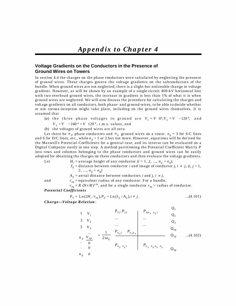
Appendix to Chapter 4
Voltage Gradients on the Conductors in the Presence ofGround Wires on TowersIn section 4.4 the charges on the phase conductors were calculated by neglecting the presenceof ground wires. These charges govern the voltage gradients on the subconductors of thebundle. When ground wires are not neglected, there is a slight but noticeable change in voltagegradient. However, as will be shown by an example of a single-circuit 400-kV horizontal linewith two overhead ground wires, the increase in gradient is less than 1% of what it is whenground wires are neglected. We will now discuss the procedure for calculating the charges andvoltage gradients on all conductors, both phase- and ground-wires, to be able to decide whetheror not corona-inception might take place, including on the ground wires themselves. It isassumed that
(a) the three phase voltages to ground are ,120,0 21 °−∠=°∠= VVVV and°∠=°−∠= 1202403 VVV , r.m.s. values, and
(b) the voltages of ground wires are all zero.Let there be pn phase conductors and gn ground wires on a tower. np = 3 for S/C lines
and 6 for D/C lines, etc., while ng = 1 or 2 but not more. However, equations will be derived forthe Maxwell's Potential Coefficients for a general case, and its inverse can be evaluated on aDigital Computer easily in one step. A method partitioning the Potential Coefficient Matrix Pinto rows and columns belonging to the phase conductors and ground wires can be easilyadopted for obtaining the charges on these conductors and then evaluate the voltage gradients.
Let Hi = average height of any conductor (i = 1, 2, ..., np + ng), Iij = distance between conductor i and image of conductor j, i ≠ j, (i, j = 1,
2, ..., np + ng)Aij = aerial distance between conductors i and j, i ≠ j,
and req = equivalent radius of any conductor. For a bundle,req = R (Nr/R)1/N, and for a single conductor req = radius of conductor.
Potential Coefficients
Pii = jiAIPrH ijijijeqi ≠= ),/(Ln),/2(Ln . ...(4.101)Charge—Voltage Relation:
0
00
...
.
.
3
2
1
3
2
1
np
g
p V
V
V
V
n
n = 02
1eπ
+++
+
ng
g
np
nnnnnn
nnn
nn
Q
Q
Q
Q
Q
Q
PP
PP
PPP
gpgpgp
ppp
gp
1
3
2
1
,1
1
)(11211
......
......
,
...(4.102)

108 Extra High Voltage AC Transmission Engineering
Here, Q1, Q2, ..., pnQ , denote the total bundle charges of N sub-conductors of the phase
conductors, while ngg QQ ,...,1 denote the total charge of the ground wires since they areinvariably single conductors. But this is a general procedure and a bundled ground conductorwill pose no special problem.
The charge coefficients, ,2/ 0eQ π can be obtained from the potential coefficients easily byinverting the potential-coefficient matrix and multiplying by the voltage matrix. Then thecharge coefficient for conductor i will be of the form
02/ eQt π = ]1201200[ 321 °∠+°−∠+°∠ MMMV , ...(4.103)where M1, M2, M3 will be combinations of elements of the matrix [M] = [P]–1, and i = 1, 2,
..., np + ng. The remaining part of the procedure for calculating the charges on individualconductors will follow equations (4.34) through (4.41) and extended to more than three conductorson the tower. Then the surface voltage gradients on all conductors, including ground wires,will follow equations (4.48), (4.51) and (4.53) through (4.58) for single conductors and bundledconductors.
Method of Matrix PartitioningThe voltage, charge and potential coefficient matrices can be partitioned into those belonging
to the phase conductors and ground wires in order to obtain the charges on all conductors, asfollows:
Let [V] = [V1, V2,..., Vnp|0, 0,..., 0]t = [[Vph], [0]]t ...(4.104)
]2/[ 0eQ π =02
1]][],[[
eQQ tgph π
...(4.105)
[P] =
][],[
][],[
gggp
pgpp
PPPP
...(4.106)
Then, obviously[Vph] = )2/1](][[]][[ 0eQPQP gpgphpp π+ ...(4.107)
[0] = )2/1](][[]][[ 0eQPQP gggphgp π+ ...(4.108)
∴ ][2
1
0gQ
eπ = ),2/1](][[][ 01 eQPP phgpgg π− − ...(4.109)
so that [Vph] = )2/1](][[]][[][ 01 eQPPPP phgpggpgpp π− −
= [Pred][Qph] (1/2πe0) ...(4.110)Therefore, the charge-coefficients on the phase conductors are
][2
1
0phQ
eπ = ]][[][][ red
1red phph VMVP =− ...(4.111)
where [Pred] and its inverse [Mred] are reduced matrices having as many rows and columnsas the number of phase conductors only, nP. Then, the charge-coefficients on the ground wiresare
][2
1
0gQ
eπ = – [Pgg]–1 [Pgp] [Mred] [Vph]
= [Mgg][Vph] ...(4.112)

Voltage Gradients of Conductors 109
We note that there is a need for inverting only the square matrix [Pgg] belonging to theground wires which will have only one number for a single ground-wire line or at the most a 2
× 2 matrix. Also the matrix product ][][ 1gpgg PP − occurs twice so that a single calculation of this
product need be carried out.Having obtained both [Qph] and [Qg] from the reduced matrices and the phase voltages, the
rest of the properties can be calculated in the usual way. We will illustrate the procedure anddiscuss some salient properties through a S/C horizontal configuration 400-kV line with twoground wires.
Example 4.16. A horizontal 400-kV line of the UPSEB in India has the following details:
Phase Conductorsm875.2sag
m8.85midspanatHeight
m875.11tower at Height=
=(single circuit, np = 3)Phase spacing 11.3 m (horizontal)Diameter 3.17 cm, 2 sub-conductors at spacing of B = 45.72 cm.
req = cm513.872.45585.1 =× .
Ground Wires Height at tower 20.875 m. Neglect sag.(2 ground wires, ng = 2) Horizontal spacing 16 m
Diameter 9.45 mm = 0.945 cm.The maximum operating voltage is 420 kV, r.m.s., line-to-line. Evaluate the following:(1) The 5 × 5 matrix of Maxwell's Potential coefficients;(2) Partition the [P]-matrix into four sub-matrices as shown before. Write down [Ppp],
[Ppg], [Pgp]and [Pgg].
(3) Evaluate the matrix ]2/[ 0eQ ph π for the charge-coefficients of the 3 phase conductors.
(4) Evaluate the matrix ]2/[ 0eQg π belonging to the ground wires. Note that even thoughthe potentials of the ground wires are zero, there exists charge on them.
(5) Calculate the surface voltage gradients on the phase conductors.(6) Calculate the same for the ground wires.(7) Calculate the above surface voltage gradients on all 3 phase conductors by neglecting
the presence of overhead ground wires, and compare them with those when groundwires are present. Give the % increase or change in surface voltage gradients whenthe ground wires are present.
(8) Calculate the corona-inception gradients on all conductors by Peek's formula takinga surface roughness factor of m = 1.3 to account for stranding. Assume air densityfactor δ = 1.
Solution. We will number the phase conductors 1, 2, 3 and the ground wires 4, 5. The
voltages are, with 3/420=V kV, (242.5 kV to ground),
V1 = 0,120,120,0 5432 ==°∠=°−∠=°∠ VVVVVVVAverage height of phase conductor = Minimum height at midspan + sag/3
= 8.85 + 2.875/3 = 9.81 m.Equivalent radius of the two-conductor bundle = 8.51 cm = 0.0851 m.


Voltage Gradients of Conductors 111
=
−
−−
46.111,6.12
6.12,46.11110 3
][][ 1gpgg PP − =
−
4.103,3.83,42
42,3.83,4.10310 3
[Ppg] [Pgg]–1[Pgp] =
−
122,123,92
123,140,123
92,123,122
10 3
[Pred] =
=− −
32.5,572.0,193.0
572.0,3.5,572.0
193.0,572.0,32.5
][]][[][ 1gpggpgpp PPPP
∴ [Mred] = [Pred]–1 =
−−−−−−
−
2.190,5.19,75.4
5.19,9.192,5.19
75.4,5.19,2.190
10 3
πππ
03
02
01
2/
2/
2/
eQeQeQ
= Vjj
j
+−−−
+×
−−−−−−
−
866.05.0
866.05.0
01
2.190,5.19,75.4
5.19,9.192,5.19
75.4,5.19,2.190
10 3
Magnitudes = [0.20273, 0.2124, 0.20273] × 242.5 kV(4) Charge Coefficients of Ground Wires
ππ
05
04
2/
2/
eQeQ
=
−−−−−−
×
−
2.190,5.19,75.4
5.19,9.192,5.19
75.4,5.19,2.190
1034.0,0833.0,042.0
042.0,0833.0,1034.010 3
Vjj
j
+−−−
+×
866.05.0
866.05.0
01
Magnitudes = 10.461 × 10⁻³ × V= 2536.8
(5) Surface Voltage Gradients on Phase Conductors
Outers: 17.3
20273.05.242 × (1 + 3.17/45.72) = 16.584 kV/cm
Centre: 16.584 × 0.2124/0.20273 = 17.375 kV/cm(6) Ground Wires
4725.010461.10 3−×
× 242.5 = 5.37 kV/cm

112 Extra High Voltage AC Transmission Engineering
(7) Without Ground Wires
[P] =
44.5,695.0,285.0
695.0,44.5,695.0
285.0,695.0,44.5
,
[M] = [P]–1 =310
187,23,9.6
23,7.189,23
9.6,23,187−
−−−−−−
Magnitude of Charge CoefficientsVeQVeQeQ 2127.02/,2025.02/2/ 020301 =π=π=π .
Gradients : Outers: 0.2025 × 242.5 (1 + 3.17/45.72)/3.17 = 16.565 kV/cmCentre : (0.2127/0.2025) 16.565 = 17.4 kV/cm
% changes: Outers: (16.584 – 16.565) × 100/16.565 = 0.115%Centre : (17.375 – 17.4) × 100/17.4 = – 0.144%
(8) Corona-inception Gradients
Phase conductors : Eop = )585.1/301.01(3.14.21 +
= 20.4 kV/cm, r.m.s.
Ground wires : Eog = )4725.0/301.01(3.14.21 +
= 23.67 kV/cmThese are above the surface voltage gradients calculated earlier. Therefore, corona
inception on any of the five conductors has not taken place. Note that the surface voltagegradients on the phase conductors has not been affected by the presence of ground wires bymore than 0.15% in this calculation.
5.1 I2R LOSS AND CORONA LOSSIn Chapter 2, the average power-handling capacity of a 3-phase e.h.v. line and percentage lossdue to I 2R heating were discussed. Representative values are given below for comparisonpurposes.System kV 400 750 1000 1150Line Length, km 400 800 400 800 400 800 400 8003-Phase MW/circuit 640 320 2860 1430 6000 3000 8640 4320(P = 0.5 V 2/xL)% Power Loss = 50 r/x 4.98% 2.4% 0.8% 0.6%kW/km Loss, 3-phase 80 20 170 42.5 120 30 130 32.5
When compared to the I2R heating loss, the average corona losses on several lines from345 kV to 750 kV gave 1 to 20 kW/km in fair weather, the higher values referring to highervoltages. In foul-weather, the losses can go up to 300 kW/km. Since, however, rain does not fallall through the year (an average is 3 months of precipitation in any given locality) andprecipitation does not cover the entire line length, the corona loss in kW/km cannot be comparedto I2R loss directly. A reasonable estimate is the yearly average loss which amounts to roughly2 kW/km to 10 kW/km for 400 km lines, and 20-40 kW/km for 800 km range since usuallyhigher voltages are necessary for the longer lines. Therefore, cumulative annual average coronaloss amounts only to 10% of I2R loss, on the assumption of continuous full load carried. Withload factors of 60 to 70%, the corona loss will be a slightly higher percentage. Nonetheless,during rainy months, the generating station has to supply the heavy corona loss and in somecases it has been the experience that generating stations have been unable to supply full ratedload to the transmission line. Thus, corona loss is a very serious aspect to be considered in linedesign.
When a line is energized and no corona is present, the current is a pure sine wave andcapacitive. It leads the voltage by 90°, as shown in Figure 5.1(a). However, when corona ispresent, it calls for a loss component and a typical waveform of the total current is as shown inFigure 5.1 (b). When the two components are separated, the resulting inphase component hasa waveform which is not purely sinusoidal, Figure 5.1 (c). It is still a current at power frequency,but only the fundamental component of this distorted current can result in power loss.
5Corona Effects-I: Power Loss and Audible Noise
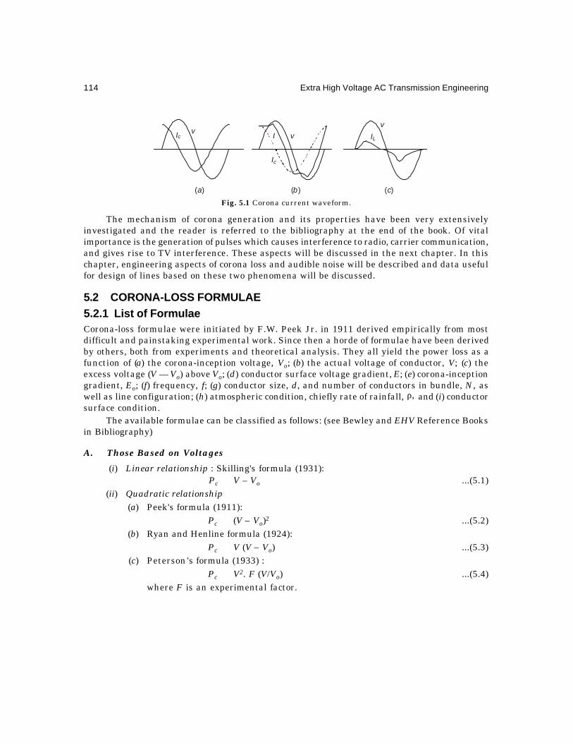
114 Extra High Voltage AC Transmission Engineering
Fig. 5.1 Corona current waveform.
The mechanism of corona generation and its properties have been very extensivelyinvestigated and the reader is referred to the bibliography at the end of the book. Of vitalimportance is the generation of pulses which causes interference to radio, carrier communication,and gives rise to TV interference. These aspects will be discussed in the next chapter. In thischapter, engineering aspects of corona loss and audible noise will be described and data usefulfor design of lines based on these two phenomena will be discussed.
5.2 CORONA-LOSS FORMULAE5.2.1 List of FormulaeCorona-loss formulae were initiated by F.W. Peek Jr. in 1911 derived empirically from mostdifficult and painstaking experimental work. Since then a horde of formulae have been derivedby others, both from experiments and theoretical analysis. They all yield the power loss as afunction of (a) the corona-inception voltage, Vo; (b) the actual voltage of conductor, V; (c) theexcess voltage (V — Vo) above Vo; (d) conductor surface voltage gradient, E; (e) corona-inceptiongradient, Eo; (f) frequency, f; (g) conductor size, d, and number of conductors in bundle, N, aswell as line configuration; (h) atmospheric condition, chiefly rate of rainfall, ,ρ and (i) conductorsurface condition.
The available formulae can be classified as follows: (see Bewley and EHV Reference Booksin Bibliography)
A. Those Based on Voltages
(i) Linear relationship : Skilling's formula (1931):Pc ∝ V – Vo ...(5.1)
(ii) Quadratic relationship(a) Peek's formula (1911):
Pc ∝ (V – Vo)2 ...(5.2)(b) Ryan and Henline formula (1924):
Pc ∝ V (V – Vo) ...(5.3)(c) Peterson's formula (1933) :
Pc ∝ V2. F (V/Vo) ...(5.4)where F is an experimental factor.
Ic v
( )a
Ic
I v
( )b
IL
v
( )c

Corona Effects-I: Power Loss and Audible Noise 115
(iii) Cubic Relationship(a) Foust and Menger formula (1928):
Pc ∝ V3 ...(5.5)(b) Prinz's formula (1940):
Pc ∝ V2 (V – Vo) ...(5.6)
B. Those Based on Voltage Gradients
(a) Nigol and Cassan formula (1961):Pc ∝ E2 In (E/Eo) ...(5.7)
(b) Project EHV formula (1966):Pc ∝ V. Em, m = 5 ...(5.8)
In order to obtain corona-loss figures from e.h.v. conductor configurations, outdoorexperimental projects are established in countries where such lines will be strung. The resultingmeasured values pertain to individual cases which depend on local climatic conditions existingat the projects. It is therefore difficult to make a general statement concerning which formulaor loss figures fit coronal losses universally. In addition to equations (5.1) to (5.8), the reader isreferred to the work carried out in Germany at the Rheinau 400 kV Research Project, inFrance at the Les Renardieres Laboratory, in Russia published in the CIGRE Proceedings from1956–1966, in Japan at the CRIEPI, in Sweden at Uppsala, and in Canada by the IREQ andOntario Hydro.
We will here quote some formulas useful for evaluating 3-phase corona loss in kW/km,which are particularly adopted for e.h.v. lines, and some which are classic but cannot be usedfor e.h.v. lines since they apply only to single conductors and not to bundles. There is noconvincing evidence that the total corona loss of a bundled conductor with N conductors is Ntimes that of a single conductor.(1) Nigol and Cassan Formula (Ontario Hydro, Canada).
Pc = K.f.r3. θ .E2. ln (E/E0), kW/km, 3-ph ...(5.9)
where f = frequency in Hz, r = conductor radius in cm.,
θ = angular portion in radians of conductor surface where the voltagegradient exceeds the critical corona-inception gradient,
E = effective surface gradient at operating voltage V, kV/cm, r.m.s.E0 = corona-inception gradient for given weather and conductor surface
condition, kV/cm, r.m.s.and K = a constant which depends upon weather and conductor surface
condition.Many factors are not taken into account in this formula such as the number of sub-
conductors in bundle, etc.(2) Anderson, Baretsky, McCarthy Formula (Project EHV, USA)An equation for corona loss in rain giving the excess loss above the fair-weather loss in kW/3-phase km is:
Pc = PFW + 0.3606 K.V.r2.ln (1 + 10 ρ ). ∑N
E3
1
5...(5.10)

116 Extra High Voltage AC Transmission Engineering
Here, PFW = total fair-weather loss in kW/km,= 1 to 5 kW/km for 500 kV, and 3 to 20 kW/km for 700 kV,
K = 5.35 × 10⁻¹⁰ for 500 to 700 kV lines,= 7.04 × 10⁻¹⁰ for 400 kV lines (based on Rheinau results),
V = conductor voltage in kV, line-line, r.m.s.,E = surface voltage gradient on the underside of the conductor, kV/cm,
peak,ρ = rain rate in mm/hour,
r = conductor radius in cm,and N = number of conductors in bundle of each phase [The factor 0.3606 =
1/1.609 3 ].Formulae are not available for (a) snow, and (b) hoar frost which are typical of Canadian
and Russian latitudes. The EHV Project suggests K = 1.27 × 10⁻⁹ for snow, but this is a highlyvariable weather condition ranging from heavy to light snow. Also, the conductor temperaturegoverns in a large measure the condition immediately local to it and it will be vastly differentfrom ground-level observation of snow.
The value of ρ to convert snowfall into equivalent rainfall rate is given as follows :Heavy snow : ρ = 10% of snowfall rate;
Medium snow : ρ = 2.5% of snowfall rate;
Light snow : ρ = 0.5% of snowfall rate.
The chief disadvantage in using formulae based upon voltage gradients is the lack ofdifinition by the authors of the formulae regarding the type of gradient to be used. As pointedout in Chapter 4, there are several types of voltage gradients on conductor surfaces in a bundle,such as nominal smooth-conductor gradient present on a conductor of the same outer radius asthe line conductor but with a smooth surface, or the gradient with surface roughness takeninto account, or the average gradient, or the average maximum gradient, and so on. It istherefore evident that for Indian conditions, an outdoor e.h.v. project is the only way of obtainingmeaningful formulae or corona-loss figures applicable to local conditions.
Later on in Section 5.3, we will derive a formula based upon charge voltage relationsduring the presence of a corona discharge.
5.2.2 The Corona CurrentThe corona loss Pc is expressed as
Pc = 3 × line-to-ground voltage × in-phase component of current.From the previously mentioned expressions for Pc, we observe that different investigators
have different formulas for the corona current. But in reality the current is generated by themovement of charge carriers inside the envelope of partial discharge around the conductor. Itshould therefore be very surprising to a discerning reader that the basic mechanism, being thesame all over the world, has not been unified into one formula for this phenomenon. We canobserve the expressions for current according to different investigators below.
1. Peek's Law. F.W. Peek, Jr., was the forerunner in setting an example for others tofollow by giving an empirical formula relating the loss in watts per unit length of conductor

Corona Effects-I: Power Loss and Audible Noise 117
with nearly all variables affecting the loss. For a conductor of radius r at a height H aboveground,
Pc = kW/km,)/1(2/1016.5 223 VVVHrf o−× − ...(5.11)
where V, Vo are in kV, r.m.s., and r and H are in metres. The voltage gradients are, at an airdensity of ,δ for a smooth conductor,
E = V/r ln (2H/r) and Eo = 21.4 )/0301.01( δ+δ r ...(5.12)
Example 5.1. For r = 1 cm, H = 5m, f = 50 Hz, calculate corona loss Pc according toPeek's formula when E = 1.1 Eo, and δ = 1.
Solution. E0 = r.ms.kV/cm,84.27)01.0/0301.01(4.21 =+
∴ E = 0316.02/.kV/cm624.301.1 0 == HrE
V = 30.624 ln (10/0.01) = 211.4 kV. (line-to-line voltage
= 211.4 3 = 366 kV)
Pc = 5.16 × 10–3 × 50 × 0.0316 × 211.42(1 – 1/1.1)2 = 2.954 kW/km≅ 3 kW/km.
The expression for the corona-loss current is
ic = Pc/V = 5.16 × 10⁻² f Hr 2/ V(1 – Vo/V )2, Amp/km ...(5.13)
For this example, ic = 3000 watts/211.4 kV = 14 mA/km.2. Ryan-Henline Formula
Pc = 4 fCV(V – V0).106, kW/km ...(5.14)Here C = capacitance of conductor to ground, Farad/m
= 02 eπ /ln (2H/r)
and V, V0 are in kV, r.ms.We can observe that the quantity (CV) is the charge of conductor per unit length. The
corona-loss current isic = 4 fC(V – V0). 106, Amp/km ...(5.15)
Example 5.2. For the previous example 5.1, compute the corona loss Pc and current icusing Ryan-Henline formulae, equations (5.14) and (5.15).
Solution. Pc = 4 × 50 × 211.42 (1 – 1/1.1) × 10–3/18 ln(1000)= 6.47 kW/km
ic = 6.47/211.4 = 3.06 × 10⁻² Amp/km = 30.6 mA/km3. Project EHV Formula. Equation (5.10).
Example 5.3. The following data for a 750 kV line are given. Calculate the corona lossper kilometre and the corona loss current.
Rate of rainfall ρ = 5 mm/hr. K = 5.35 × 10⁻¹⁰, PFW = 5 kW/km
V = 750 kV, line-to-line. H = 18 m, S = 15 m phase spacing

118 Extra High Voltage AC Transmission Engineering
N = 4 sub-conductors each of r = 0.0175 m with bundle spacing
B = 0.4572 m. (Bundle radius R = B/ 2 = 0.3182 m). Use surface voltagegradient on centre phase for calculation.
Solution. From Mangoldt Formula, the gradient on the centre phase conductor will be
E = V.[1 + (N – 1) r/R]/[N.r. ln 2H/req 1)/2( 2 +SH ]
where req = R (N.r/R)1/N. Using the values given,
E = 18.1 kV/cm, r.m.s., = 18.1 2 peak = 25.456Pc = 5 + 0.3606 × 5.35 × 10–10 × 750 × 0.1752 × ln(1 + 50) × 12 × (25.456)5
= 5 + 229 = 234 kW/km, 3-phaseThe current is
ic = A/km54.03750/2343/ ==VPc .
Note that the increase in loss under rain is nearly 46 times that under fair weather.Comparing with Table on page 127 the corona loss is much higher than the I2R heating loss.
5.3 CHARGE-VOLTAGE (q – V ) DIAGRAM AND CORONA LOSS
5.3.1 Increase in Effective Radius of Conductor and Coupling FactorsThe partial discharge of air around a line conductor is the process of creation and movement ofcharged particles and ions in the vicinity of a conductor under the applied voltage and field. Weshall consider a simplified picture for conditions occurring when first the voltage is passingthrough the negative half-cycle and next the positive half-cycle, as shown in Figure 5.2.
Fig. 5.2 Space-charge distribution in corona and increase in effective radius of conductor
In Figure 5.2(a), free electrons near the negative conductor when repelled can acquiresufficient energy to form an electron avalanche. The positive ions (a neutral molecule whichhas lost an electron) are attracted towards the negative conductor while the electrons drift intolower fields to attach themselves to neutral atoms or molecules of Nitrogen and Oxygen toform negative ions. Some recombination could also take place. The energy imparted for causinginitial ionization by collision is supplied by the electric field. During the positive half cycle, thenegative ions are attracted towards the conductor, but because of local conditions not all ionsdrift back to the conductor. A space charge is left behind and the hysteresis effect gives rise tothe energy loss. Furthermore, because of the presence of charged particles, the effective charge
–
–
–+
( )b
r
r0
E0
( )c
EquivalentCorona Envelope
( )a
–
–
––
+++

Corona Effects-I: Power Loss and Audible Noise 119
of the conductor ground electrode system is increased giving rise to an increase in effectivecapacitance. This can be interpreted in an alternative manner by assuming that the conductordiameter is effectively increased by the conducting channel up to a certain extent where theelectric field intensity decreases to a value equal to that required for further ionization, namely,the corona-inception gradient, Figure 5.2(c).
Example 5.4. A single smooth conductor 1 cm in radius is strung 5 metres above ground;using Peek's formula for corona-inception gradient, find
(a) the corona-inception voltage,(b) the equivalent radius of conductor to the outside of the corona envelope at 20%
overvoltage. Take .1=δSolution.
(a) E0 = m./kV2784cm/kV84.27)/0301.01(4.21 ==+ r
∴ V0 = 01.0/10ln(01.02784)/2(ln..0 ××=rHrE )= 192.3 kV, r.m.s.
(b) Let r0 = effective radius of the corona envelope
Then, E0c = )/)0301.01(2140 0r+ , and
1.2 × 192.3 = E0c.ro.ln (2H/ro) giving
230.8 = 2140 (1 + 0.0301/ )./10(ln.). 000 rrrA trial solution yields r0 = 0.0126 m = 1.26 cm.So far we have considered power-frequency excitation and worked with effective or r.m.s.
values of voltage and voltage gradient. There are two other very important types of volltage,namely the lightning impulse and switching surge, which give rise to intense corona on theconductors. The resulting energy loss helps to attenuate the voltage magnitudes during travelfrom a source point to other points far away along the overhead line. The resulting attenuationor decrease in amplitude, and the distortion or waveshape will be discussed in detail in the nextsection. We mention here that at power frequency, the corona-inception gradient and voltageare usually higher by 10 to 30% of the operating voltage in fair weather so that a line is notnormally designed to generate corona. However, local conditions such as dirt particles etc., dogive rise to some corona. On the other hand, under a lightning stroke or a switching operation,the voltage exceeds twice the peak value of corona-inception voltage. Corona plumes have beenphotographed from actual lines which extend up to 1.2 metres from the surface of the conductor.Therefore, there is evidence of a very large increase in effective diameter of a conductor underthese conditions.
Corona-inception gradients on conductors under impulse conditions on cylindricalconductors above a ground plane are equal to those under power frequency but crest valueshave to be used in Peek's formula. The increase in effective radius will in turn change thecapacitance of the conductor which has an influence on the voltage coupled to the other phase-conductors located on the same tower. The increased coupling factor on mutually-coupledtravelling waves was recognized in the 1930's and 40's under lightning conditions. At present,switching surges are of great concern in determining insulation clearance between conductorand ground, and conductor to conductor. We will consider the increase in diameter and theresulting coupling factors under both types of impulses.

120 Extra High Voltage AC Transmission Engineering
Example 5.5. A single conductor 2.5 inch in diameter of a 525-kV line (line-to-line voltage)is strung 13 m above ground. Calculate (a) the corona-inception voltage and (b) the effectiveradius of conductor at an overvoltage of 2.5 p.u. Consider a stranding factor m = 1.25 forroughness. (c) Calculate the capacitance of conductor to ground with and without corona. (d) Ifa second conductor is strung 10 m away at the same height, calculate the coupling factors inthe two cases. Take .1=δ
Solution. r = 0.03176 m, H = 13.(a) E0r = 2140 × 0.8 (1 + 03176.0/0301.0 )
= 2001 kV/m = 20 kV/cm.V0 = E0.r. ln (2H/r) = 532.73 kV r.m.s., line-to-ground,
= 753.4 kV peak.At 525 kV, r.m.s., line-to-line, there is no corona present.
(b) 2.5 p.u. voltage = 3/25255.2 × = 1071.65 kV, crest.
Therefore, corona is present since the corona-onset voltage is 753.4 kV, crest.When considering the effective radius, we assume a smooth surface for the envelopeso that
1071.65 = 3000 )./26(ln.)./0301.01( 000 rrr+
A trial and error solution yields r0 = 0.05 metre. This is an increase
in radius of 0.05 – 0.03176 = 0.01824 metre or 57.43%.
(c) C = )./2(ln/2 0 rHeπ
Without corona, C = 8.282 nF/km;
With corona, C = 8.88 nF/km,
(d) The potential coefficient matrix is
[P] = ∆
−
−==
− 1,
,][][and
,
,
1121
12221
2221
1211
PPPP
PMPPPP
where ∆ = |[P]|, the determinant.The self-capacitance is ∆π /2 110 Pe while the mutual capacitance is – ./2 12 ∆π Peo The
coupling factor is K12 = – P12/P11.
Without corona K12 = – ln )03176.0/26(ln/)10/1026( 22 +
= – 1.0245/6.7076 = – 0.15274With corona, K12 = – 1.0245/ ln (26/.05) = – 0.1638.
This is an increase of 7.135%.
For bundled conductors, coupling factors between 15% to 25% are found in practice. Notethat with a switching surge of 1000 kV crest, the second conductor experiences a voltage ofnearly 152 kV crest to ground so that the voltage between the conductors could reach 850 kVcrest.

Corona Effects-I: Power Loss and Audible Noise 121
5.3.2 Charge-Voltage Diagram with CoronaWhen corona is absent the capacitance of a conductor is based on the physical radius of themetallic conductor. The charge-voltage relation is a straight line OA as shown in Figure 5.3and C = q0/V0, where V0 = the corona-inception voltage and q0 the corresponding charge. However,beyond this voltage there is an increase in charge which is more rapid than given by the slopeC of the straight-line q0 — V0 relation. This is shown as the portion AB which is nearly straight.When the voltage is decreased after reaching a maximum Vm there is a hysteresis effect andthe q – V relation follows the path BD. The slope of BD almost equals C showing that the space-charge cloud near the conductor has been absorbed into the conductor and charges far enoughaway from the conductor are not entirely pulled back. The essential properties of the q –Vdiagram for one half-cycle of an ac voltage or the unipolar lightning and switching impulses canbe obtained from the trapezoidal area OABD which represents the energy loss.
Fig. 5.3 Charge-Voltage diagram of corona.
Let the slope of AB equal (1 + K) C where K is an experimental factor which lies between0.6 and 0.8 having an average value of 0.7. The maximum charge correspondihg to Vm is denoted
as qm. The area of OABD equals )(21 2
02 VVKC m − as shown below:
Area OABD = (Area DOFB) – (Area OAG) – Area (GAHF) – Area (AHB)
= (Area DOFB) – )()(21
)(21
000000 VVqqVVqVq mmm −−−−−
= Area DOFB – )(21
00 VVqVq mmm −+ ...(5.16)
Now, BH = ,/)()1( 0000 VVVqKqq mm −+=−
JH = ,/)( 000 VVVq m −
and BF = ,/)()1( 0000 VVVqKqq mm −++=
∴ DO = BJ = BH – JH = ./)( 000 VVVKq m − ...(5.17)
Area DOFB = 02
0000 /21
/)()(21
VVqVVVVKqVBFDO mmmm +−=+ ...(5.18)
Area OAG = ).(Area;21
0000 VVqAGFHVq m −=
Area AHB = 02
0002
02
000 /)(21
/)(21
))((21
VVVKqVVVqVVqq mmmm −+−=−− ...(5.19)
qm
q0
V0 Vm
B
J
H
FG
A
C
O
D
(1 + )K C

122 Extra High Voltage AC Transmission Engineering
∴ Areas (OAG + AGFH + AHB) = ],)()[/(21 2
02
00 VVKVVq mm −+ ...(5.20)
Finally, Area OABD = 0000 /))((.21
VVVVVqK mm +−
= )(21 2
02 VVKC m − ...(5.21)
For a unipolar waveform of voltage the energy loss is equal to equation (5.21). For an acvoltage for one cycle, the energy loss is twice this value.
∴ Wac = 20
2( VVKC m − ) ...(5.22)
The corresponding power loss will be
Pc = f Wac = )( 20
2 VVfKC m − ...(5.23)
If the maximum voltage is very close to the corona-inception voltage V0, we can write
),(2)()( 00020
2 VVVVVVVVV mmmmm −=−+=− so that
Pc = )(2 0VVKCVf mm − ...(5.24)
where all voltages are crest values. When effective values for Vm and V0 are used.Pc = )(4 0VVVKCf − ...(5.25)
This is very close to the Ryan-Henline formula, equation (5.14) with K = 1. For lightning
and switching impulses the energy loss is equation (5.21) which is W = )(21 2
02 VVKC m − where all
voltages are crest values.Example 5.6. An overhead conductor of 1.6 cm radius is 10 m above ground. The normal
voltage is 133 kV r.m.s. to ground (230 kV, line-to-line). The switching surge experienced is 3.5p.u. Taking K = 0.7, calculate the energy loss per km of line. Assume smooth conductor.
Solution. C = )/2(ln/2 0 rHeπ = 7.79 nF/km
E0 = )016.0/0301.01(30 + = 37.14 kV/cm, crest
∴ V0 = E0.r. ln (2H/r) = 423.8 kV, crest
Vm = 21335.3 × = 658.3 kV, crest
∴ W = 0.5 × 0.7 × 7.79 × 10–9 (658.32 – 423.82) × 106 Joule/km= 0.7 kJ/km.
This property will be used in deriving attenuation of travelling waves caused by lightningand switching in Chapter 8.
5.4 ATTENUATION OF TRAVELLING WAVES DUE TO CORONA LOSSA voltage wave incident on a transmission line at an initial point x = 0 will travel with a velocityv such that at a later time t the voltage reaches a point x = vt from the point of incidence, asshown in Figure 5.4 In so doing if the crest value of voltage is higher than the corona-disruptivevoltage for the conductor, it loses energy while it travels and its amplitude decreasescorresponding to the lower energy content. In addition to the attenuation or decrease inamplitude, the waveshape also shows distortion. In this section, we will discuss only attenuation
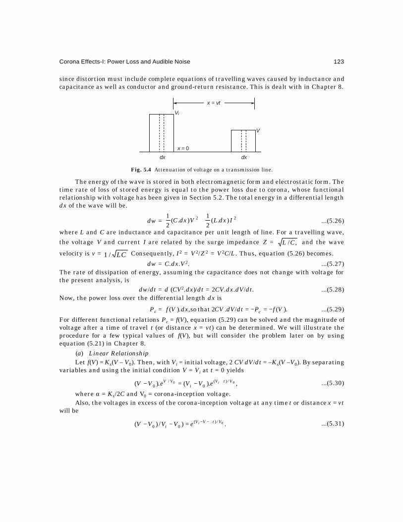
Corona Effects-I: Power Loss and Audible Noise 123
since distortion must include complete equations of travelling waves caused by inductance andcapacitance as well as conductor and ground-return resistance. This is dealt with in Chapter 8.
Fig. 5.4 Attenuation of voltage on a transmission line.
The energy of the wave is stored in both electromagnetic form and electrostatic form. Thetime rate of loss of stored energy is equal to the power loss due to corona, whose functionalrelationship with voltage has been given in Section 5.2. The total energy in a differential lengthdx of the wave will be.
dw = 22 ).(21
).(21
IdxLVdxC + ...(5.26)
where L and C are inductance and capacitance per unit length of line. For a travelling wave,
the voltage V and current I are related by the surge impedance Z = ,/CL and the wave
velocity is v = LC/1 Consequently, I2 = V2/Z2 = V2C/L. Thus, equation (5.26) becomes.
dw = C.dx.V2. ...(5.27)The rate of dissipation of energy, assuming the capacitance does not change with voltage forthe present analysis, is
dw/dt = d (CV2.dx)/dt = 2CV.dx.dV/dt. ...(5.28)Now, the power loss over the differential length dx is
Pc = ).(/.2thatso,).( VfPdtdVCVdxVf c −=−= ...(5.29)
For different functional relations Pc = f(V), equation (5.29) can be solved and the magnitude ofvoltage after a time of travel t (or distance x = vt) can be determined. We will illustrate theprocedure for a few typical values of f(V), but will consider the problem later on by usingequation (5.21) in Chapter 8.
(a) Linear RelationshipLet f(V) = Ks(V – V0). Then, with Vi = initial voltage, 2 CV dV/dt = –Ks(V –V0). By separating
variables and using the initial condition V = Vi at t = 0 yields
,).().( 00 /)(0
/0
VtVi
VV ieVVeVV ∝−=− ...(5.30)
where α = Ks/2C and V0 = corona-inception voltage.Also, the voltages in excess of the corona-inception voltage at any time t or distance x = vt
will be
.)/)( 0/)(00
VtVVi
ieVVVV ∝−−=−− ...(5.31)
x = vt
Vi
x = 0
dx dx
V

124 Extra High Voltage AC Transmission Engineering
This expression yields an indirect method of determining α = Ks /2C by experiment, ifdistortion is not too great. It requires measuring the incident wave magnitude Vi and themagnitude V after a time lapse of t or distance x = vt at a different point on the line, whosecorona-inception voltage V0 is known. When C is also known, the constant Ks is calculated.
Example 5.7. A voltage with magnitude of 500 kV crest is incident on a conductor whosecorona-inception voltage is 100 kV crest, and capacitance C = 10 nF/km. After a lapse of 120 sµ
(36 km of travel at light velocity) the measured amplitude is 110 kV. Calculate α and Ks.Solution. Vi/V0 = .400,10,5 00 =−=− VVVV i
V0 = volts10kV100 5=
∴ 10/400 = )10/10120(exp]100/)110500([exp 56 a××−− −
This gives 19 secvolt10325.62/ −−×==α CKs .
∴ Ks = 5.126101010325.62 99 =×××× − watts/km-volt or Amp/km.
(b) Quadratic Formula(i) Let the loss be assumed to vary as
f(V) = KR V(V –V0) ...(5.32)So that
2CV (dV/dt) = – KR V(V – V0).With V = Vi at t = 0, integration gives
])2/([exp0
0 tCKVVVV
Ri
−=−−
...(5.33)
The voltage in excess of corona-inception value behaves as if it is attenuated by a resistanceof R per unit length as given by the formula
])2/([exp).()( 00 tLRVVVV i −−=−
∴ KR = .// 2ZRLRC =For the previous example.
KR = .105.6110
400ln.
10120
102 66
9−
−
−×=
××
The units are watts/km-volt2.(ii) If the loos is assumed to vary as
f(V) = )( 20
2 VVKQ − ...(5.34)
then 2CV (dV/dt) = .0with)( 20
2 ==−− tatVVVVK iQ
∴ 20
20
2
2
V
V
V
V
i −
− = exp [– (KQ /C)t]
For the previous example,
KQ = .10395100
100
110
500ln.
10120
1010 62
2
2
2
6
9−
−
−×=
−−
××

Corona Effects-I: Power Loss and Audible Noise 125
(iii) Let .)()( 20VVKVf P −= Then,
.0atwith)()/.(2 20 ==−−= tVVVVKdtdVCV iP
This gives
tCKVVVV
VVVVVVV
Pi
ii )2/())((
)(ln
00
0
0
0 =−−
−+
−−
...(5.35)
For 90 1010,kV110,kV500,kV100 −×==== CVVV i F/km, and
610120 −×=t sec, there results Kp = 224 × 10–6.
(c) Cubic Relation
If f(V) = 33 )/(2,. VKdtdVCVVK cc −=giving Vi /V = .)2/(1 tVCK ic+ ...(5.36)For the previous example, Kc = 1.182 × 10⁻⁹ watts/km-volt3.
5.5 AUDIBLE NOISE: GENERATION AND CHARACTERISTICSWhen corona is present on the conductors, e.h.v. lines generate audible noise which is especiallyhigh during foul weather. The noise is broadband, which extends from very low frequency toabout 20 kHz. Corona discharges generate positive and negative ions which are alternatelyattracted and repelled by the periodic reversal of polarity of the ac excitation. Their movementgives rise to sound-pressure waves at frequencies of twice the power frequency and its multiples,in addition to the broadband spectrum which is the result of random motions of the ions, asshown in Figure 5.5. The noise has a pure tone superimposed on the broadband noise. Due todifferences in ionic motion between ac and dc excitations, dc lines exhibit only a broadbandnoise, and furthermore, unlike for ac lines, the noise generated from a dc line is nearly equalin both fair and foul weather conditions. Since audible noise (AN) is man-made, it is measuredin the same manner as other types of man-made noise such as aircraft noise, automobileignition noise, transformer hum, etc. We will describe meters used and methods of ANmeasurements in a subsequent section 5.7.
Fig. 5.5 Audible Noise frequency spectra from ac and dc transmission lines.
Audible noise can become a serious problem from 'psycho-acoustics' point of view, leadingto insanity due to loss of sleep at night to inhabitants residing close to an e.h.v. line. This
0 100 200
AN ANdB dB
f
AC Line
f
DC Line
126 Extra High Voltage AC Transmission Engineering
problem came into focus in the 1960's with the energization of 500 kV lines in the USA.Regulatory bodies have not as yet fixed limits to AN from power transmission lines since suchregulations do not exist for other man-made sources of noise. The problem is left as a social onewhich has to be settled by public opinion. The proposed limits for AN are discussed in the nextsection.
5.6 LIMITS FOR AUDIBLE NOISESince no legislation exists setting limits for AN for man-made sources, power companies andenvironmentalists have fixed limits from public-relations point of view which power companieshave accepted from a moral point of view. In doing so, like other kinds of interference, humanbeings must be subjected to listening tests. Such objective tests are performed by every civic-minded power utility organization. The first such series of tests performed from a 500-kV lineof the Bonneville Power Administration in the U.S.A. is known as Perry Criterion. The ANlimits are as follows:
No complaints : Less than 52.5 dB (A),Few complaints : 52.5 dB (A) to 59 dB (A),Many complaints : Greater than 59 dB (A),The reference level for audible noise and the dB relation will be explained later. The
notation (A) denotes that the noise is measured on a meter on a filter designated as A-weightingnetwork. There are several such networks in a meter.
Design of line dimensions at e.h.v. levels is now governed more by the need to limit ANlevels to the above values. The selection of width of line corridor or right-of-way (R-O-W),where the nearest house can be permitted to be located, if fixed from AN limit of 52.5 dB(A),will be found adequate from other points of view at 1000 to 1200 kV levels. The design aspectwill be considered in Section 5.8. The audible noise generated by a line is a function of thefollowing factors:
(a) the surface voltage gradient on conductors,
(b) the number of sub-conductors in the bundle,
(c) conductor diameter,
(d) atmospheric conditions, and
(e) the lateral distance (or aerial distance) from the line conductors to the point wherenoise is to be evaluated.
The entire phenomenon is statistical in nature, as in all problems related to e.h.v. linedesigns, because of atmospheric conditions.
While the Perry criterion is based upon actual listening experiences on test groups ofhuman beings, and guidelines are given for limits for AN from an e.h.v. line at the location ofinhabited places, other man-made sources of noise do not follow such limits. A second criterionfor setting limits and which evaluates the nuisance value from man-made sources of AN iscalled the 'Day-Night Equivalent' level of noise. This is based not only upon the variation of ANwith atmospheric conditions but also with the hours of the day and night during a 24-hourperiod. The reason is that a certain noise level which can be tolerated during the waking hoursof the day, when ambient noise is high, cannot be tolerated during sleeping hours of the nightwhen little or no ambient noises are present. This will be elaborated upon in Section 5.9.According to the Day-Night Criterion, a noise level of 55 dB(A) can be taken as the limit instead

Corona Effects-I: Power Loss and Audible Noise 127
of 52.5 dB(A) according to the Perry Criterion. From a statistical point of view, these levels areconsidered to exist for 50% of the time during precipitation hours. These are designated as L50levels.
5.7 AN MEASUREMENT AND METERS
5.7.1 Decibel Values in AN and Addition of SourcesAudible noise is caused by changes in air pressure or other transmission medium so that it isdescribed by Sound Pressure Level (SPL). Alexander Graham Bell established the basic unitfor SPL as 20 × 10–6 Newton/m2 or 20 micro Pascals [2 × 10⁻⁵ micro bar]. All decibel values arereferred to this basic unit. In telephone work there is a flow of current in a set of head-phonesor receiver. Here the basic units are 1 milliwatt across 600 ohms yielding a voltage of 775 mVand a current of 1.29 mA. For any other SPL, the decibel value is
SPL(dB) = 10 Log10 (SPL/20 × 10–6) Pascals ...(5.37)This is also termed the 'Acoustic Power Level', denoted by PWL, or simply the audible
noise level, AN.
Example 5.8. The AN level of one phase of a 3-phase transmission line at a point is 50dB. Calculate (a) the SPL in Pascals; (b) if a second source of noise contributes 48dB at thesame location, calculate the combined AN level due to the two sources.
Solution.
(a) 10 Log10 (SPL1/2 × 10–5) = 50, which gives
SPL1 = 2 × 10–5 × 1050/10 = 2 Pascals
(b) Similarly, SPL2 = 2 × 10–5 × 10 48/10 = 1.262 Pascals
∴ Total SPL = SPL1 + SPL2 = 3.262 Pascals.The decibel value will be
AN = 10 Log10 (SPL/2 ×10–5) = 52.125 dB.Consider N sources whose decibel values, at a given point where AN level is to be evaluated,
are AN1, AN2,...., ANN. In order to add these sources and evaluate the resultant SPL and dBvalues, the procedure is as follows:
The individual sound pressure levels are
SPL1 =10/AN6
210/AN6 21 101020SPL,101020 ××=×× −− etc.
∴ The total SPL = SPL1 + SPL2 + . . . = 2 × 10⁻⁵ ∑=
N
i
i
1
10/AN10 ...(5.38)
The decibel value of the combined sound pressure level is
AN = 10 Log10 (SPL/2 × 10–5) = 10 Log10 ∑=
N
i
i
1
AN1.010 ...(5.39)
Example 5.9. A 3-phase line yields AN levels from individual phases to be 55 dB, 52 dB,and 48 dB. Find the resulting AN level of the line.
Solution. 58.42.55.5AN1.0AN1.0AN1.0 10382.5101010101010 321 ×=++=++
∴ AN = .dB31.57)10382.5(Log10 510 =×

128 Extra High Voltage AC Transmission Engineering
5.7.2 MicrophonesInstruments for measurement of audible noise are very simple in construction in so far as theirprinciples are concerned. They would conform to standard specifications of each country, as forexample, ANSI, ISI or I.E.C., etc. The input end of the AN measuring system consists of amicrophone as shown in the block diagram, Figure 5.6. There are three types of microphonesused in AN measurement from e.h.v. lines and equipment. They are (i) air-condenser type;(ii) ceramic; and (iii) electret microphones. Air condenser microphones are very stable andexhibit highest frequency response. Ceramic ones are the most rugged of the three types.Since AN is primarily a foul-weather phenomenon, adequate protection of microphone fromweather is necessary. In addition, the electret microphone requires a polarization voltage sothat a power supply (usually battery) will also be exposed to rain and must be protected suitably.
Fig. 5.6 Block diagram of AN Measuring Circuit.
Some of the microphones used in AN measurement from e.h.v. lines are General RadioType 1560-P, or 1971-9601, or Bruel and Kjor type 4145 or 4165, and so on. The GR type has aweather protection. Since AN level form a transmission line is much lower than, say, aircraft
or ignition noise, 1" (2.54 cm) diameter microphones are used although some have used "21
ones, since these have more sensitivity than 1" microphones. Therefore, size is not thedetermining factor.
The most important characteristic of a microphone is its frequency response. In makingAN measurements, it is evident that the angle between the microphone and the source is notalways 90° so that the grazing angle determines the frequency response. Some typicalcharacteristics are as shown in Figure 5.7.
Fig. 5.7 Response of microphone for grazing and perpendicular incidence.
MIKE
Pre-Amp II Amp A B C
WeightingNetworks
Output Amp. Meter
Output Amp.
OutputJack
Gain ControlCalibration
Grazing
Perpendicular
Ideal
4
0
5
dB
102 103 104
Frequency, Hz104103102
0
Mike DirectedTowards Cond.
Mike Vertical
IdealNon-Directional
Frequency, Hz

Corona Effects-I: Power Loss and Audible Noise 129
AN levels are statistical in nature and long-term measurements are carried out byprotecting the microphone from rain, wind, animals, and birds. Some types of shelters usewind-screens with a coating of silicone grease. Foam rubber wind-covers have also been usedwhich have negligible attenuation effect on the sound, particularly on the A-weighted networkwhich will be described below. Every wind-cover must also be calibrated and manufacturerssupply this data. Foam-rubber soaks up rain and must be squeezed out periodically and siliconegrease applied.
5.7.3 Weighting NetworksThere are 5 weighting networks designated as A to E in Sound Pressure Level Meters. The 'A'weighted network has been designed particularly to have nearly the same response as thehuman ear, while the 'C' weighted network has a flat response up to 16 kHz. The 'A' networkis also least susceptible to wind gusts. It is also preferred by Labour Relations Departments forassessing the adversity of noise-created psychological and physiological effects in noisyenvironments such as factories, power stations, etc.
Typical frequency response of the A, B, C weighting networks are sketched in Figure5.8(a) while 5.8(b) compares the responses of A, D networks. The A-weighting network is widelyused for relatively nondirectional sources. From these curves it is seen that the C-networkprovides essentially flat response from 20 Hz to 10 kHz. The human ear exhibits such flatresponse for sound pressure levels up to 85 dB or more. At lower SPL, the human ear does nothave a flat response with frequency and the A and B networks are preferred. The A network isused for SPL up to 40 dB and the B for SPL up to 70 dB. Sometimes, the A-weighted network isknown as the 40 dB network. It is also used for transformer noise measurements.
Fig. 5.8 Frequency responses of (a) A, B, C weighting networks, (b) A, D weighting networks.
5.7.4 Octave Band and Third Octave BandIt was mentioned earlier that in addition to the broadband noise generated by corona, puretones at double the power frequency and its multiples exist. These discrete-frequency componentsor line spectra are measured on octave bands by selective filters. Figure 5.9 shows a schematicdiagram of the switching arrangement for use with a 50-Hz line.
A
B
C
A
B,C
10 10
0 10
– 10 – 10
– 20 – 20
– 30 – 30
– 40 – 40
dB dB
102 102103 103104 104
Frequency, Hz Frequency, Hz
A
D
D
A
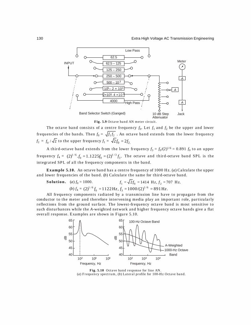
130 Extra High Voltage AC Transmission Engineering
Fig. 5.9 Octave band AN meter circuit.
The octave band consists of a centre frequency f0. Let f1 and f2 be the upper and lower
frequencies of the bands. Then f0 = 21 ff . An octave band extends from the lower frequency
f2 = 2/0f to the upper frequency f1 = .20 22 ff =
A third-octave band extends from the lower frequency f3 = f0/(2)1/6 = 0.891 f0 to an upper
frequency f4 = .)2(1225.1.)2( 33/1
006/1 fff == The octave and third-octave band SPL is the
integrated SPL of all the frequency components in the band.
Example 5.10. An octave band has a centre frequency of 1000 Hz. (a) Calculate the upperand lower frequencies of the band. (b) Calculate the same for third-octave band.
Solution. (a) f0 = 1000. ∴ .Hz707,H14142 201 === fzff
(b) f4 = .H891)2/(1000,H1122)2( 6/130
6/1 zfzf ===All frequency components radiated by a transmission line have to propagate from the
conductor to the meter and therefore intervening media play an important role, particularlyreflections from the ground surface. The lowest-frequency octave band is most sensitive tosuch disturbances while the A-weighted network and higher frequency octave bands give a flatoverall response. Examples are shown in Figure 5.10.
Fig. 5.10 Octave band response for line AN.(a) Frequency spectrum, (b) Lateral profile for 100-Hz Octave band.
High Pass
A
A
A
Meter
Jack10 dB StepAttenuator
Band Selector Switch (Ganged)
INPUT
Low Pass
62.5
4000
62.5 – 125
125 – 250
250 – 500
500 – 10 3
10 – 2 × 1033
2×10– 4 ×10 33
65
60
55
50
45
40
dB
102 103 104
Frequency, Hz
65
60
55
50
45
40
dB
102 103 104
Frequency, Hz
100-Hz Octave Band
A-Weighted1000-Hz Octave
Band

Corona Effects-I: Power Loss and Audible Noise 131
Thus, displacing the microphone even a few metres can give erroneous results on a 100-Hz octave band. The curve is caused by standing waves and reflections from the ground surface.
5.8 FORMULAE FOR AUDIBLE NOISE AND USE IN DESIGNAudible noise from a line is subject to variation with atmospheric condition. This means thatthere is no one quantity or AN level that can be considered as the audible noise level of a line.All designers accept two levels–the L50 level and the L5 level. These are defined as follows:L50 Level: This is the AN level as measured on the A-weighted network which is exceeded 50%of the time during periods of rain, usually extending over an entire year.L5 Level: Similar to L50, but exceeded only 5% of the total time.
The L5 level is used for describing the noise levels in heavy rain which are generated inartificial rain tests. These are carried out in 'cage tests' where artificial rain apparatus is used,as well as from short outdoor experimental lines equipped with such apparatus. Many empiricalformulas exist for calculating the AN level of an e.h.v. line [see IEEE Task Force paper, October1982]. However, we will discuss the use of the formula developed by the B.P.A. of the USA. Itis applicable for the following conditions:
(a) All line geometries with bundles having up to 16 sub-conductors.
(b) Sub-conductor diameters in the range 2 cm to 6.5 cm.
(c) The AN calculated is the L50 level in rain.
(d) Transmission voltages are 230 kV to 1500 kV, 3-phase ac.Referring to Figure 5.11, the AN level of each phase at the measuring point M is, with
i = 1, 2, 3,AN (i) = 120 log10 Eam (i) + 55 log10 d – 11.4 log10 D(i) – 115.4, dB(A) (5.40)
Fig. 5.11 Calculation of AN level of line by B.P.A. Formula.
It applies for N < 3 sub-conductors in the bundles. For N ≥ 3, the formula becomesAN(i) = 120 log10 Eam(i) + 55 log10 d – 11.4 log10 D(i)
+ 26.4 log10 N – 128.4, dB(A) ...(5.41)Here, Eam(i) = average maximum surface voltage gradient on bundle belonging to
phase i in kV/cm, r.m.s.d = diameter of sub-conductor in cm.,N = number of sub-conductors in bundle,
and D(i) = aerial distance from phase i to the location of the microphone in metres.
1
2
3
D1
D2 D3
M

132 Extra High Voltage AC Transmission Engineering
When all dimensions are in metre units, the above giveN < 3 : AN(i) = 120 log Em(i) + 55 log dm – 11.4 log D(i) + 234.6, dB(A) ...(5.42)
N ≥ 3 : AN(i) = 120 log Em(i) + 55 log dm – 11.4 log D(i)+ 26.4 log N + 221.6, dB(A) ...(5.43)
Having calculated the AN level of each phase, the rule for addition of the three levelsfollows equation (5.39),
AN = )(dB,10log103
1
)(1.010 A
i
iAN∑=
...(5.44)
For a double-circuit line, the value of i extends from 1 to 6.We observe that the AN level depends on the following four quantities:(i) the surface voltage gradient on conductor,
Fig. 5.14 AN level of 1150 kV line (calculated).
(ii) the conductor diameter,
(iii) the number of sub-conductors in bundle, and
Fig. 5.12 AN level of 400 kV line (calculated). Fig. 5.13 AN level of 735 kV line (calculated).
56
54
52
50
480 1 2 3
dB(A
)
400 kV
L-Type
Horizontal
X/H0
48
50
52
54
56
58
60
1 2 3
dB(A
)
4 × 0.0302
735 kVHydro-Quebec
Line
X/H
4 × 0.0403
50
49
48
47
46
45
44
dB(A
)
B.P.A. 1150 kV Line
0 1 2 3
X
44 = 26H
X/H
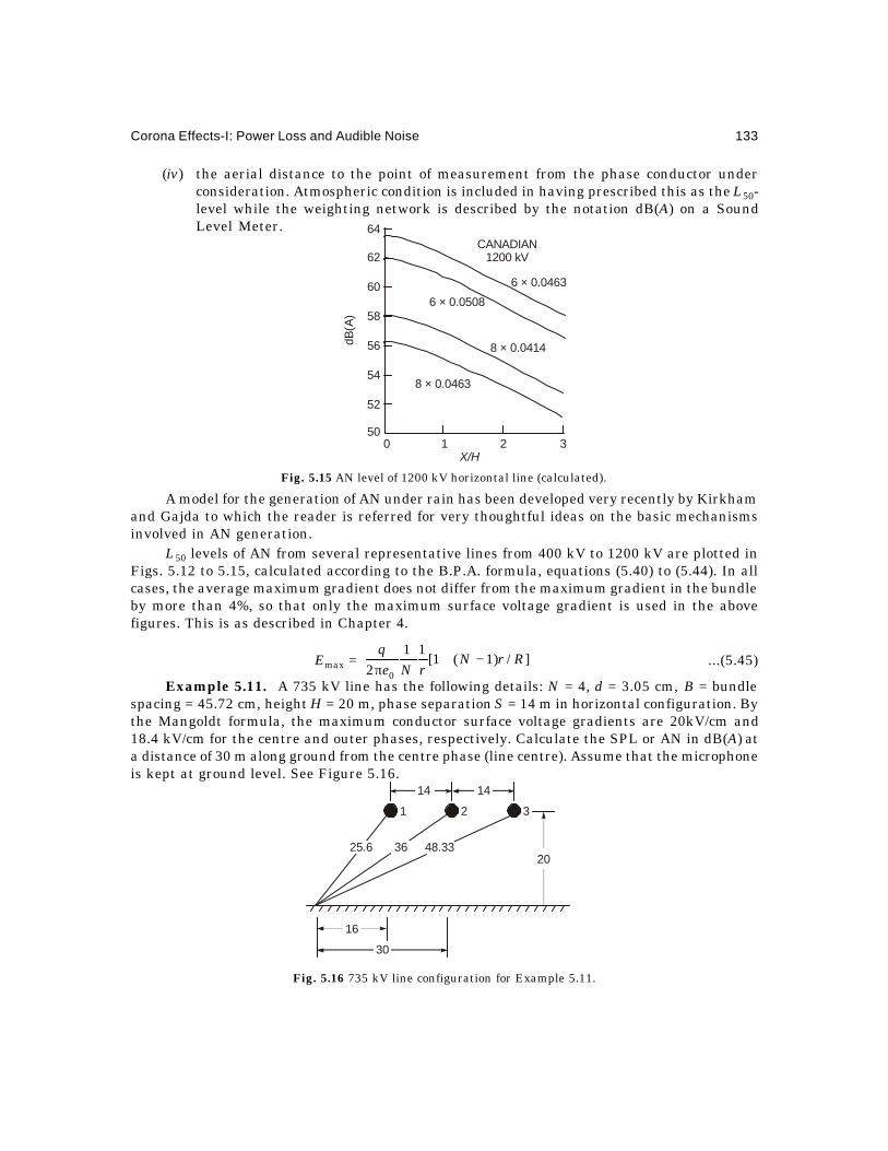
Corona Effects-I: Power Loss and Audible Noise 133
(iv) the aerial distance to the point of measurement from the phase conductor underconsideration. Atmospheric condition is included in having prescribed this as the L50-level while the weighting network is described by the notation dB(A) on a SoundLevel Meter.
Fig. 5.15 AN level of 1200 kV horizontal line (calculated).
A model for the generation of AN under rain has been developed very recently by Kirkhamand Gajda to which the reader is referred for very thoughtful ideas on the basic mechanismsinvolved in AN generation.
L50 levels of AN from several representative lines from 400 kV to 1200 kV are plotted inFigs. 5.12 to 5.15, calculated according to the B.P.A. formula, equations (5.40) to (5.44). In allcases, the average maximum gradient does not differ from the maximum gradient in the bundleby more than 4%, so that only the maximum surface voltage gradient is used in the abovefigures. This is as described in Chapter 4.
Emax = ]/)1(1[11
2 0
RrNrNe
q−+
π...(5.45)
Example 5.11. A 735 kV line has the following details: N = 4, d = 3.05 cm, B = bundlespacing = 45.72 cm, height H = 20 m, phase separation S = 14 m in horizontal configuration. Bythe Mangoldt formula, the maximum conductor surface voltage gradients are 20kV/cm and18.4 kV/cm for the centre and outer phases, respectively. Calculate the SPL or AN in dB(A) ata distance of 30 m along ground from the centre phase (line centre). Assume that the microphoneis kept at ground level. See Figure 5.16.
Fig. 5.16 735 kV line configuration for Example 5.11.
0 1 2 3
64
62
60
58
56
54
52
50
CANADIAN1200 kV
6 × 0.0463
6 × 0.0508
8 × 0.0414
8 × 0.0463
X/H
dB(A
)
30
16
25.6 36 48.33
14 14
1 2 3
20
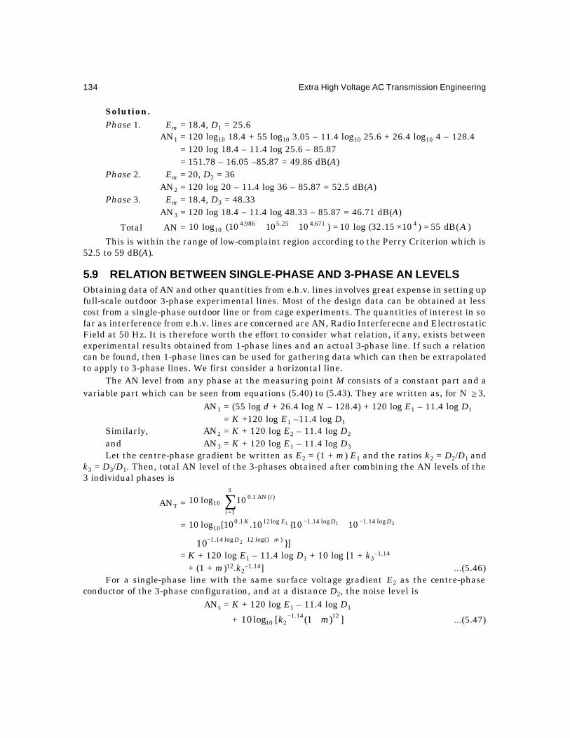
134 Extra High Voltage AC Transmission Engineering
Solution.
Phase 1. Em = 18.4, D1 = 25.6AN1 = 120 log10 18.4 + 55 log10 3.05 – 11.4 log10 25.6 + 26.4 log10 4 – 128.4
= 120 log 18.4 – 11.4 log 25.6 – 85.87= 151.78 – 16.05 –85.87 = 49.86 dB(A)
Phase 2. Em = 20, D2 = 36AN2 = 120 log 20 – 11.4 log 36 – 85.87 = 52.5 dB(A)
Phase 3. Em = 18.4, D3 = 48.33AN3 = 120 log 18.4 – 11.4 log 48.33 – 85.87 = 46.71 dB(A)
∴ Total AN = )(dB55)1015.32(log10)101010(log10 4671.425.5986.410 A=×=++
This is within the range of low-complaint region according to the Perry Criterion which is52.5 to 59 dB(A).
5.9 RELATION BETWEEN SINGLE-PHASE AND 3-PHASE AN LEVELSObtaining data of AN and other quantities from e.h.v. lines involves great expense in setting upfull-scale outdoor 3-phase experimental lines. Most of the design data can be obtained at lesscost from a single-phase outdoor line or from cage experiments. The quantities of interest in sofar as interference from e.h.v. lines are concerned are AN, Radio Interferecne and ElectrostaticField at 50 Hz. It is therefore worth the effort to consider what relation, if any, exists betweenexperimental results obtained from 1-phase lines and an actual 3-phase line. If such a relationcan be found, then 1-phase lines can be used for gathering data which can then be extrapolatedto apply to 3-phase lines. We first consider a horizontal line.
The AN level from any phase at the measuring point M consists of a constant part and avariable part which can be seen from equations (5.40) to (5.43). They are written as, for N ≥ 3,
AN1 = (55 log d + 26.4 log N – 128.4) + 120 log E1 – 11.4 log D1
= K +120 log E1 –11.4 log D1
Similarly, AN2 = K + 120 log E2 – 11.4 log D2
and AN3 = K + 120 log E1 – 11.4 log D3
Let the centre-phase gradient be written as E2 = (1 + m) E1 and the ratios k2 = D2/D1 andk3 = D3/D1. Then, total AN level of the 3-phases obtained after combining the AN levels of the3 individual phases is
ANT = ∑=
3
1
)(AN1.010 10log10
i
i
= 311 log14.1log14.1log121.010 101010.10[log10 DDEK −− +
]10 )1(log12log14.1 2 mD ++−+= K + 120 log E1 – 11.4 log D1 + 10 log [1 + k3
–1.14
+ (1 + m)12.k2–1.14] ...(5.46)
For a single-phase line with the same surface voltage gradient E2 as the centre-phaseconductor of the 3-phase configuration, and at a distance D2, the noise level is
ANs = K + 120 log E1 – 11.4 log D1
+ ])1([log10 1214.1210 mk +− ...(5.47)

Corona Effects-I: Power Loss and Audible Noise 135
Therefore, the difference in AN levels of equation (5.46) and (5.47) is
ANT – ANs = 1214.12
1214.12
14.13
10)1(
)1(1log10
mkmkk
++++
−
−−
...(5.48)
This is the decibel adder which will convert the single-phase AN level to that of a 3-phaseline.
Example 5.12. Using equation (5.46) compute ANT for the 735 kV line of example 5.11.Solution. K = – 85.87, 1 + m = 20/18.4 = 1.087.
11.4 log D1 = 16.05, 120 log E1 = 151.8, k2 = 36/25.6 = 1.406,k3 = 48.33/25.6 = 1.888
∴ 33.3)1(1 1214.12
14.13 =+++ −− mkk
ANT = – 85.87 + 151.8 – 16.05 + 10 log 3.33 = 55.1 dB(A).
Example 5.13. Using equation (5.48). compute the decibel adder to convert the single-phase AN level of the centre phase to the three-phase AN level of examples 5.11 and 5.12.
Solution.
8054.18444.133.3
)1(
)1(11214.1
2
1214.12
14.13 ==
++++
−
−−
mkmkk
∴ dB adder = 10 log 1.8054 = 2.566.The AN level of the centre phase was 52.5 dB(A) at 30 m from the conductor along ground.
This will be the level of a single-phase line with the same surface voltage gradient and distanceto the location of microphone.
∴ ANT = ANs + dB adder = 52.5 + 2.566 = 55.07 dB(A)
5.10 DAY-NIGHT EQUIVALENT NOISE LEVELIn previous discussions the AN level of a transmission line has been chosen as the L50 value orthe audible noise in decibels on the A-weighted network that is exceeded for 50% of the durationof precipitation. This has been assumed to give an indication of the nuisance value. However,another criterion which is actively followed and applied to man-made AN sources is called theDay-Night Equivalent Noise level. This has found acceptance to aircraft noise levels, heavyroad traffic noise, ignition noise, etc., which has led to litigation among many aggrieved partiesand the noise makers. According to this criterion, certain sound level might be acceptableduring day-time hours when ambient noises will be high. But during the night-time hours thesame noise level from a power line or other man-made sources could be found objectionablebecause of the absence of ambient noises. The equivalent annoyance during nights is estimatedby adding 10 dB(A) to the day-time AN level, or, in other words, by imposing a 10 dB (A)penalty.
Consider an L50 level of a power line to be AN and the day-time to last for D hours. Then,the actual annoyance level for the entire 24 hours is computed as a day-night equivalent levelas follows:
Ldn = )(dB,10).24(10.241
log10 )10AN(1.0AN1.010 ADD
−+ + ...(5.49)
This is under the assumption that the level AN is present throughout the 24 hours.

136 Extra High Voltage AC Transmission Engineering
Example 5.14. The L50 level of a line is 55 dB(A). The day-light hours are 15 and night-time is 9 hours in duration. Calculate the day-night equivalent and the decibel adder to the day-time AN level.
Solution. Ldn = )(dB4.61)1091015(241
Log10 5.65.510 A=
×+×
The decibel adder is 61.4 – 55 = 6.4 dB(A).An addition of 6.4 dB increases the SPL by 4.365 times [10 log 4.365 = 6.4]. The nuisance
value of the line has been increased by 6.4 dB(A) by adding 10 dB(A) penalty for night hours.If the day-night hours are different from 15 and 9, a different decibel adder will be necessary.
The 10 dB(A) penalty added to night time contributes 6 times the AN value as the day-timelevel, since.
.615/901015/109 5.55.6 ==××In evaluating the nuisance value of AN from an e.h.v. line, we are only concerned with
the duration of rainfall during a day and not the total day-night hours or 24 hours. If rain is notpresent over the entire 24 hours but only for a certain percentage of the day and night, thenthe day-night equivalent value of AN is calculated as shown below. Let it be assumed that
pd = % of duration of rainfall during the day time,and pn = % of duration of rainfall during the night.
Then, Ldn = )100/)(24(10).100/)(24/1[(10 AN1.010 nd pDDpLog −+
]10 )10AN(1.0 + ...(5.50)
Example 5.15. The following data are given for a line : L50 = 55 dB(A). D = 15, pd = 20, pn= 50. Calculate the day-night equivalent of AN and the dB-adder.
Solution. Duration of rain is 3 hours during the day and 4.5 hours during the night.
∴ Ldn = )]105.09102.015)(24/1[(Log10 5.65.510 ××+××
= 58 dB(A).
The decibel adder is 3 dB(A).
Now, the night-time contribution is 15 times that during the day time (4.5 × 106.5/3 × 105.5
= 45/3 = 15).In the above equation (5.50), it was assumed that the L50 levels for both day and night
were equal, or in other words, the precipitation characteristics were the same. If this is not thecase, then the proper values must be used which are obtained by keeping very careful record ofrainfall rates and AN levels. Such experiments are performed with short outdoor experimentallines strung over ground, or in 'cages'.
5.11 SOME EXAMPLES OF AN LEVELS FROM EHV LINESIt might prove informative to end this chapter with data on the performance of some e.h.v. linedesigns based upon AN limits from all over the world.
(1) The B.P.A. in the U.S.A. has fixed 50 dB(A) limit for the L50 noise level at 30 m fromthe line centre in rain for their 1150 kV line operating at 1200 kV.
(2) The A.E.P., U.H.V. Project of the E.P.R.I., and several other designs fall very closeto the above values.

Corona Effects-I: Power Loss and Audible Noise 137
(3) Operating 750 kV lines of the A.E.P. in U.S.A. gave 55.4 dB(A) at 760 kV. The samecompany performed experiments from short outdoor line at Apple Grove and obtained56.5 dB(A) at 775 kV, proving that short-line data can be relied upon to provide adequatedesign values.
(4) The Hydro-Quebec company of Canada has given the following calculated AN levelsat 30.5 m from the centres of their proposed line designs.
Voltage, kV 525 735Conductor size 2 × 1.602" 3 × 1.302" 4 × 1.382" 4 × 1.2"Bundle spacing 18" 18" 18" 18"Phase spacing 34' 34' 50' 45'AN Level, dB(A) 57 52 55 58.5
Review Questions and Problems
1. Describe the behaviour of space-charge effects inside a corona envelope and discusswhy load current cannot flow in a conductor inside this envelope even though it is aconducting zone.
2. Derive the expression )(21 2
02 VVKCP mc −= for the energy loss from the charge-voltage
diagram, Figure 5.3.3. It was theorized by E.W. Boehne, the famous electrical engineer and professor at
M.I.T., that the increase in effective radius of conductor and consequent increase incapacitance was partly responsible for attenuation of travelling waves on conductorsdue to lightning. From the material given in this chapter, discuss why this theory isvalid.
4. A 400 kV line supplies a load of 600 MW over a distance of 400 km. Its conductors are2×3.18 cm dia. with a resistance of 0.03 ohm/km per phase. It carries an average loadof 400 MW over the year (66.7% load factor).
(a) Calculate annual energy loss of the line.
(b) If the average corona loss is 20 kW/km for the 3-phases for 2 months of the year,calculate the annual energy loss due to corona.
(c) Calculate the % corona energy loss as compared to the I2R heating loss of theline.
5. Describe the difference between a line spectrum and band spectrum for noise. Whatis the difference between a pure tone and broad-band spectrum?
6. For the 735-kV line of problem 2 in Chapter 4, calculate the AN level at a distance of15 metres along ground from the outer phase.
7. Using this as the AN level of the line, calculate the day-night equivalent if daytime is15 hours and the penalty for night is 8 dB(A) instead of the suggested 10 dB(A) in thetext.

6.1 CORONA PULSES: THEIR GENERATION AND PROPERTIESThere are in general two types of corona discharge from transmission-line conductors: (i)Pulseless or Glow Corona; (ii) Pulse Type or Streamer Corona. Both these give rise to energyloss, but only the pulse-type of corona gives interference to radio broadcast in the range of 0.5MHz to 1.6 MHz. In addition to corona generated on line conductors, there are spark dischargesfrom chipped or broken insulators and loose guy wires which interfere with TV reception in the80–200 MHz range. Audible noise has already been discussed in Chapter 5 which is caused byrain drops and high humidity conditions. Corona on conductors also causes interference toCarrier Communication and Signalling in the frequency range 30 kHz to 500 kHz.
In the case of Radio and TV interference the problem is one of locating the receivers farenough from the line in a lateral direction such that noise generated by the line is low enoughat the receiver location in order to yield a satisfactory quality of reception. In the case ofcarrier interference, the problem is one of determining the transmitter and receiver powers tocombat line-generated noise power.
In this section we discuss the mechanism of generation and salient characteristics of onlypulse-type corona in so far as they affect radio reception. As in most gas discharge phenomenaunder high impressed electric fields, free electrons and charged particles (ions) are created inspace which contain very few initial electrons. We can therefore expect a build up of resultingcurrent in the conductor from a zero value to a maximum or peak caused by the avalanchemechanism and their motion towards the proper electrode. Once the peak value is reachedthere is a fall in current because of lowering of electric field due to the relatively heavy immobilespace charge cloud which lowers the velocity of ions. We can therefore expect pulses to begenerated with short crest times and relatively longer fall times. Measurements made of singlepulses by the author in co-axial cylindrical arrangement are shown in Figure 6.1 under dcexcitation. Similar pulses occur during the positive and negative half-cycles under ac excitation.The best equations that fit the observed wave shapes are also given on the figures. It will beassumed that positve corona pulses have the equation
i+ = )( ttp eeik β−α−
+ − ...(6.1)
while negative pulses can be best described by
i– =tt
p etik δ−γ−−−
/2/3 . ...(6.2)
6Corona Effects-II: Radio Interference

Corona Effects-II: Radio Interference 139
These equations have formed the basis for calculating the response of bandwidth-limited radioreceivers (noise meters), and for formulating mathematical models of the radio-noise problem.In addition to the waveshape of a single pulse, their repetition rate in a train of pulses is alsoimportant.
Fig. 6.1 Single positive and negative pulses
i+ =)/(5.1.);( tt
ptt
p etikieeik δ−γ−−−−
β−α−+ ⋅=−
Referring to Fig. 6.2, when a conductor is positive with respect to ground, an electronavalanche moves rapidly into the conductor leaving the heavy positive-ion charge cloud close tothe conductor which drifts away. The rapid movement of electrons and motion of positive-ionsgives the steep front of the pulse, while the further drift of the positive-ion cloud will form thetail of the pulse. It is clear that the presence of positive charges near the positive conductorlowers the field to an extent that the induced current in the conductor nearly vanishes. As soonas the positive-ions have drifted far enough due to wind or neutralized by other agencies suchas free electrons by recombination, the electric field in the vicinity of the conductor regainssufficiently high value for pulse formation to repeat itself. Thus, a train of pulses results froma point in corona on the conductor. The repetition rate of pulses is governed by factors local tothe conductor. It has been observed that only one pulse usually occurs during a positive halfcycle in fair weather and could increase to about 10 in rain where the water sprays resultingfrom breaking raindrops under the applied field control electrical conditions local to the conductor.
Fig. 6.2 Formation of pulse train from positive polarity conductor.
The situation when the conductor is negative with respect to ground is the reverse of thatdescribed above. The electron avalanche moves away from the conductor while the positive-ioncloud moves towards the negatively-charged conductor. However, since the heavy positive-ionsare moving into progressively higher electric fields, their motion is very rapid which gives riseto a much sharper pulse than a positive pulse. Similarly, the lighter electrons move rapidlyaway from the conductor and the electric field near the conductor regains its original value for
Positive Pulse
Negative Pulse
ip
ip
0 100 200 300
2.35 (i ep t–0.0105
– e– 0.03465 t)
ns
651 . . i tp –3/2 e– (34.86 + 0.01215)/t t
++
–
( )a ( )b ( )c
Pulse Train
( )d
Pulse Formation
+ ++ +

140 Extra High Voltage AC Transmission Engineering
the next pulse generation quicker than for the positive case. Therefore, negative pulses aresmaller in amplitude, have much smaller rise and fall times but much higher repetition ratesthan positive pulses. It must at once be evident that all the properties of positive and negativepulses are random in nature and can only be described through random variables.
Typical average values of pulse properties are as follows:
Type Time to Time to 50% Peak Value Repetition RateCrest on Tail of Current Pulses per Second
A.C. D.C.Positive 50 ns 200 ns 100 mA Power Freq. 1,000Negative 20 ns 50 ns 10 mA 100 × P.F. 10,000
Pulses are larger as the diameter of conductor increases because the reduction in electricfield strength as one moves away from the conductor is not as steep as for a smaller conductorso that conditions for longer pulse duration are more favourable. In very small wires, positivepulses can be absent and only a glow corona can result, although negative pulses are presentwhen they are known as Trichel Pulses named after the first discoverer of the pulse-typedischarge. Negative pulses are very rarely important from the point of view of radio interferenceas will be described under "Radio Noise Meter Response" to corona pulses in Section 6.2.Therefore, only positive polarity pulses are important because of their larger amplitudes eventhough their repetition rate is lower than negative pulses.
6.1.1 Frequency SpectrumThe frequency spectrum of radio noise measured from long lines usually corresponds to theFourier Amplitude Spectrum (Bode Amplitude Plot) of single pulses. These are shown inFigure 6.3. The Fourier integral for a single double-exponential pulse is
F (jw) = ∫ ∫∞
∞−
−β−α−− −=to
jwtttp
jwt dteeeKidtetf0
.).(.).(
= )]/(1)/(1[ jwjwKip +β−+α
= ))(/()( jwjwKip +β+αα−β
Fig. 6.3 Bode frequency plot of positive and negative corona pulses.
The amplitude is
A (w) = ))((/).(. 2222 wwiK p +β+αα−β ...(6.4)
0
– 5
– 10
– 15
– 20
– 250 2 4 6 8 10
– Pulse
+ Pulse
Frequency, MHz
dB


142 Extra High Voltage AC Transmission Engineering
6.2 PROPERTIES OF PULSE TRAINS AND FILTER RESPONSERadio Interference (RI) level is governed not only by the amplitude and waveshape of a singlepulse but also by the repetitive nature of pulses in a train. On an ac transmission line, asmentioned earlier, positive pulses from one single point in corona occur once in a cycle or atthe most 2 or 3 pulses are generated near the peak of the voltage. In rain, the number of pulsesin one positive half cycle shows an increase. Therefore, the number of pulses per second on a50 Hz line from a single point in fair weather ranges from 50 to 150 and may reach 500 in rain.Since there exist a very large number of points in corona, and the pulses occur randomly intime without correlation, the frequency spectrum is band-type and not a line spectrum. It isalso found that in fair weather there exists a certain shielding effect when one source in coronadoes not permit another within about 20 to 50 cm. This is verified by photographs taken atnight when plumes of bluish discharges occur at discrete points. However, in rain, there is acontinuous luminous envelope around a conductor. It is therefore a matter of some difficulty inactually ascertaining the repetition rate of pulses as seen by the input end of a noise meter,which is either a rod antenna or a loop antenna. Fortunately, this is not as serious as it looks,since the integrated response of a standard noise-meter circuit is practically independent of thepulse repetition rate if the number of pulses per second (pps) is less than the bandwidth frequencyof the filter in the meter weighting circuit. This is discussed below for a simple case of rectangularpulses with periodic repetition. The analysis can be extended to include finally the actual caseof randomly-occurring pulse trains with double-exponential shape. But this is a highly advancedtopic suitable for experts involved in design of noise meters. [See Begamudre, Trans. Can. Eng.Inst., Oct. 1970].
Consider Figure 6.4 showing rectangular pulses of amplitude A and width τ having aperiodic time T and repetition frequency f = 1/T pulses per second. When this is an evenfunction the Fourier Series for this type of pulse train contains only cosine terms. The amplitudeof any harmonic is
F(k) = ∫τ τπ
π=π
0
2sin
24
2cos4
Tk
kAdtkftA
T ...(6.8)
Fig. 6.4 (a) Pulse train: Amplitude A, width ,τ period T.
(b) Ideal bandwidth-limited filter with centre frequency fo and bandwidth .f∆
∆ f
f0
FILTER
( )b
τ
T T T
PULSES
( )a
A

Corona Effects-II: Radio Interference 143
The Fourier Series is
F(w) = ∑∞
=
τπ
π1
cos2
sin24
k
kwtTk
kA
...(6.9)
Let such a signal be passed through an ideal filter with bandwidth f∆ and steep cut-off, asshown in Fig. 6.4(b). Then, the number of harmonics passed will be.
N = ../ Tfff ∆=∆ ...(6.10)
If the meter is tuned to a centre frequency f0 = nf, the output will contain harmonic terms
from .21
to21
+
−= NnNnk The output of the filter is then.
τ
+π
+π
τ
−π
−πf
Nn
NnA
fN
nNn
A2
2sin1
24
to2
2sin1
24
21
21
Certain approximations can be made to obtain a workable expression when we considerwhat happens in an actual situation in practice. The tuned frequency is about f0 = 1 MHz andthe repetition frequency f can be considered as f = 1000 pps. The meter bandwidth is 5 kHz forANSI meters and 9 kHz for CISPR meters of European design. Therefore.
n = .100010/10/ 360 ==ff
Since the bandwidth is 5 kHz and the harmonics of the pulse train are separated by 1000Hz, only 5 or 6 harmonic components will pass in the 5 kHz bandwidth. For f∆ = 9 kHz, about9 or 10 harmonic components will pass. Thus, (n – N/2) and (n + N/2) range from 997 to 1003and we can approximate both these with a value of 1000 which is f0/f. The output of the filterwill then be the sum of harmonic terms such as
τ
∆+πτ
∆−ππ 2
2sinto2
2sin24
000
ffffffA
where the pulse width τ is of the order of 100 ns = 10–7.
Now,
τ
∆π−τπ
222sin 0
ff = .
22sin.2cos
22cos.2sin 00 τ
∆πτπ−τ
∆πτπ
ff
ff ...(6.11)
Since ,1015710250022
2 57 −− ×=××π≈τ∆
πf
we can write cos .02
2sinand12
2 =τ∆
π=τ∆
πff
Then, the output of the filter will be nearly
tffNffA
000
2cos.2sin...24
πτππ ...(6.12)
where we have introduced the time function of equation (6.9). The final output can also bewritten as
tffffA
000
2cos.2sin.24
πτπ∆
π ...(6.13)
since ,fNf ∆= the bandwidth, according to (6.10).
144 Extra High Voltage AC Transmission Engineering
The output of the filter is a cosine wave at frequency f0, the tuned frequency (1 MHz, say),and is modulated by the amplitude
τπ∆
π 00
2sin..2
fffA
= τπτπ
∆τ=πττπ
τπ∆
π 0
0
0
0
22sin
).).((4)2(2
2sin..
2f
ffA
ff
fA
...(6.14)
For low tuned frequencies, the sigma factor τπ
τπ
0
0
22sinf
f is nearly 1. Thus, at low frequencies
f0, the response of the filter is nearly flat and rolls off at higher frequency. The following salientproperties can also be noted from equation (6.14).
(1) The response of the filter is directly proportional to =τ)(A area of the pulse.
(2) The response is proportional to =∆ )( f bandwidth, provided the number of harmonicspassed is very low.
(3) The response is proportional to the Si-factor.That the response of the filter is flat up to a certain repetition frequency of pulses is not
surprising since as the repetition frequency increases, the tuned frequency becomes a lowerorder harmonic of the fundamental frequency with resulting higher amplitude. But there is acorresponding reduction in the number of harmonics passed in the bandwidth of the filtergiving an output which is nearly equal to that obtained at a lower tuned frequency. Therefore,changes in repetition frequency of the pulses in a train affect the noise level only to a smalldegree.
Since the amplitude-duration product of the pulse determines the output, it is evidentthat a positive corona pulse yields much higher noise level than a negative corona pulse. Inpractice, we omit negative-corona generated radio interference.
6.3 LIMITS FOR RADIO INTERFERENCE FIELDSRadio Interference (RI) resulting from a transmission line is a man-made phenomenon and assuch its regulation should be similar to other man-made sources of noise as mentioned inChapter 5, such as audible noise, automobile ignition noise, aircraft noise, interference fromwelding equipment, r–f heating equipment etc. Some of these are governed by IS 6842.Legislation for fixing limits to all these noise sources is now gaining widespread publicity andawareness in public in order to protect the environment from all types of pollution, includingnoise. Interference to communication systems is described through Signal-to-Noise Ratiodesignated as S/N Ratio, with both quantities measured on the same weighting circuit of asuitable standard meter. However, it has been the practice to designate the signal from abroadcast station in terms of the average signal strength called the Field Intensity (FI) settingof the field-strength meter, while the interference signal to a radio receiver due to line noise ismeasured on the Quasi-Peak (QP) detector circuit. The difference in weighting circuits will bediscussed later on. There are proposals to change this custom and have both signal and noisemeasured on the same weighting circuit. This point is mentioned here in order that the readermay interpret S/N ratios given by public utility organizations in technical literature or elsewheresince interference problems result in expensive litigations between contesting parties.
As mentioned earlier, it is the duty or responsibility of a designer to keep noise level froma line below a limiting value at the edge of the right-of-way (R-O-W) of the line corridor. Thevalue to be used for this RI limit is causing considerable discussion and, we shall describe twopoints of view currently used in the world. Some countries, particularly in Europe, have set
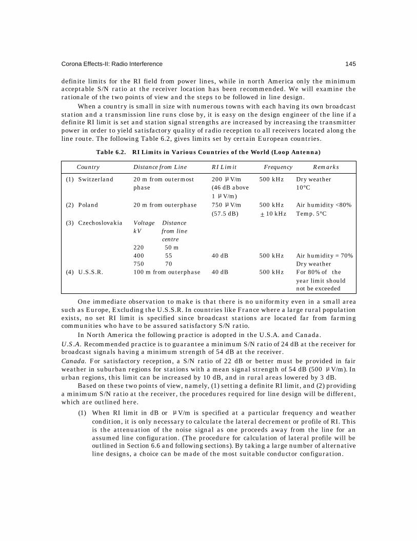
Corona Effects-II: Radio Interference 145
definite limits for the RI field from power lines, while in north America only the minimumacceptable S/N ratio at the receiver location has been recommended. We will examine therationale of the two points of view and the steps to be followed in line design.
When a country is small in size with numerous towns with each having its own broadcaststation and a transmission line runs close by, it is easy on the design engineer of the line if adefinite RI limit is set and station signal strengths are increased by increasing the transmitterpower in order to yield satisfactory quality of radio reception to all receivers located along theline route. The following Table 6.2, gives limits set by certain European countries.
Table 6.2. RI Limits in Various Countries of the World (Loop Antenna)
Country Distance from Line RI Limit Frequency Remarks
(1) Switzerland 20 m from outermost 200 µ V/m 500 kHz Dry weatherphase (46 dB above 10°C
1 µ V/m)(2) Poland 20 m from outerphase 750 µ V/m 500 kHz Air humidity <80%
(57.5 dB) ± 10 kHz Temp. 5°C(3) Czechoslovakia Voltage Distance
kV from line centre220 50 m400 55 40 dB 500 kHz Air humidity = 70%750 70 Dry weather
(4) U.S.S.R. 100 m from outerphase 40 dB 500 kHz For 80% of theyear limit shouldnot be exceeded
One immediate observation to make is that there is no uniformity even in a small areasuch as Europe, Excluding the U.S.S.R. In countries like France where a large rural populationexists, no set RI limit is specified since broadcast stations are located far from farmingcommunities who have to be assured satisfactory S/N ratio.
In North America the following practice is adopted in the U.S.A. and Canada.U.S.A. Recommended practice is to guarantee a minimum S/N ratio of 24 dB at the receiver forbroadcast signals having a minimum strength of 54 dB at the receiver.Canada. For satisfactory reception, a S/N ratio of 22 dB or better must be provided in fairweather in suburban regions for stations with a mean signal strength of 54 dB (500 µ V/m). Inurban regions, this limit can be increased by 10 dB, and in rural areas lowered by 3 dB.
Based on these two points of view, namely, (1) setting a definite RI limit, and (2) providinga minimum S/N ratio at the receiver, the procedures required for line design will be different,which are outlined here.
(1) When RI limit in dB or µ V/m is specified at a particular frequency and weathercondition, it is only necessary to calculate the lateral decrement or profile of RI. Thisis the attenuation of the noise signal as one proceeds away from the line for anassumed line configuration. (The procedure for calculation of lateral profile will beoutlined in Section 6.6 and following sections). By taking a large number of alternativeline designs, a choice can be made of the most suitable conductor configuration.
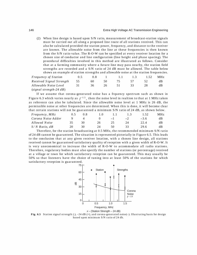
146 Extra High Voltage AC Transmission Engineering
(2) When line design is based upon S/N ratio, measurement of broadcast-station signalsmust be carried out all along a proposed line route of all stations received. This canalso be calculated provided the station power, frequency, and distance to the receiverare known. The allowable noise from the line at these frequencies is then knownfrom the S/N ratio value. The R-O-W can be specified at every receiver location for achosen size of conductor and line configuration (line height and phase spacing). Theprocedural difficulties involved in this method are illustrated as follows. Considerthat at a farming community where a future line may pass nearby, the station fieldstrengths are recorded and a S/N ratio of 24 dB must be allowed. The table belowshows an example of station strengths and allowable noise at the station frequencies.
Frequency of Station 0.5 0.8 1 1.1 1.3 1.52 MHzReceived Signal Strength 55 60 50 75 57 52 dBAllowable Noise Level 31 36 26 51 33 28 dB(signal strength-24 dB)
If we assume that corona-generated noise has a frquency spectrum such as shown inFigure 6.3 which varies nearly as ,5.1−f then the noise level in realtion to that at 1 MHz takenas reference can also be tabulated. Since the allowable noise level at 1 MHz is 26 dB, thepermissible noise at other frequencies are determined. When this is done, it will become clearthat certain stations will not be guaranteed a minimum S/N ratio of 24 dB, as shown below.
Frequency, MHz 0.5 0.8 1.0 1.1 1.3 1.52 MHzCorona Noise Adder 9 4 0 –1 –2 –3.6 dBAllowed Noise 35 30 26 25 24 22.4 dBS/N Ratio, dB 20 30 24 50 33 29.6 dB
Therefore, for the station broadcasting at 0.5 MHz, the recommended minimum S/N ratioof 24 dB cannot be guaranteed. The situation is represented pictorially in Figure 6.5. This leadsto the conclusion that at any given receiver location, with a chosen line design, all stationsreceived cannot be guaranteed satisfactory quality of reception with a given width of R-O-W. Itis very uneconomical to increase the width of R-O-W to accommodate all radio stations.Therefore, regulatory bodies must also specify the number of stations (or percentage) receivedat a village or town for which satisfactory reception can be guaranteed. This may usually be50% so that listeners have the choice of tuning into at least 50% of the stations for whichsatisfactory reception is guaranteed.
Fig. 6.5 Station signal strength (.), –24 dB (×), and corona-generated noise(–). Illustrating basis for designbased upon minimum S/N ratio of 24 db.
75
60
45
30
15
00 0.5 1.0 1.5
Station Strengths
CoronaNoise
∝f – 1.5
dB
Frequency, MHz
x – (Station Strength – 24 dB)

Corona Effects-II: Radio Interference 147
This process has to be repeated at all villages and towns or other locations such as militaryestablishments, etc., along the proposed line route and a best compromise for line designarrived at. Once a definite RI limit is set at a fixed lateral distance from the line as controlledby the S/N ratio, which in the above example was 26 dB at 1 MHz at the edge of R-O-W, the linedesign follows similar lines as for case (1) where the limit is specified to start with underlegislation of the country.
Referring to Fig 6.5, any X-mark falling below the corona-generated noise curve representsa station for which the minimum S/N ratio of 24 dB cannot be obtained. Therefore, quality ofreception for such a station at the receiver location will be unsatisfactory.
6.4 FREQUENCY SPECTRUM OF THE RI FIELD OF LINEThe frequency spectrum of radio noise refers to the variation of noise level in µV or µ V/m (ortheir dB values referred to 1 µ V or 1µ V/m) with frequency of measurement. The frequency-spectrum of a single corona pulse of double-exponential shape was found in Section 6.1 to be
A(w) = ))((/).(. 2222 wwiK p +β+αα−β ...(6.14)
On a long line, there exist a very large number of points in corona and a noise meterlocated in the vicinity of the line (usually at or near ground level) responds to a train of pulsesoriginating from them. The width of a single pulse is about 200 ns (0.2 µs) while the separationof pulses as seen by the input end of the meter could be 1 sµ or more. Therefore, it is unusualfor positive pulses to overlap and the noise is considered as impulsive. When pulses overlap,the noise is random. Measurements indicate that from a long line, the RI frequency spectrumfollows closely.
RI(w) ∝ f–1 to f–1.5 ...(6.15)Thus, at 0.5 MHz the noise is 6-9 dB higher than at 1 MHz, while at 2 MHz it is 6–9 dB
lower. In practice, these are the adders suggested to convert measured noise at any frequencyto 1 MHz level. The frequency spectrum is therefore very important in order to convert noiselevels measured at one frequency to another. This happens when powerful station signalinterferes with noise measurements from a line so that measurements have to be carried outat a frequency at which no broadcast station is radiating. The frequency spectrum from corona-generated line noise is nearly fixed in its characteristic so that any deviation from it as measuredon a noise meter is an indication of sources other than the line, which is termed "backgroundnoise". In case a strong source of noise is present nearby, which is usually a factory withmotors that are sparking or a broken insulator on the tower, this can be easily recognized sincethese usually yield high noise levels up to 30 MHz and their frequency spectrum is relativelyflat.
6.5 LATERAL PROFILE OF RI AND MODES OF PROPAGATIONThe most important aspect of line design from interference point of view is the choice of conductorsize, number of sub-conductors in bundle, line height, and phase spacing. Next in importance isthe fixing of the width of line corridor for purchase of land for the right-of-way. The lateraldecrement of radio noise measured at ground level as one moves away from the line has theprofile sketched in Fig. 6.6. It exhibits a characteristic double hump within the space betweenthe conductors and then decreases monotonically as the meter is moved away from the outer

148 Extra High Voltage AC Transmission Engineering
phase. For satisfactory radio reception, a limit RIi is determined as explained in the previoussection. No receiver should be located within the distance d0 from the outer phase or dc fromthe line centre. Therefore, it becomes essential to measure or to be able to calculate at designstages the lateral profile very accurately from a proposed line in order to advise regulatorybodies on the location of receivers. In practice, many complaints are heard from the public whoexperience interference to radio broadcasts if the line is located too close to their homesteadswhen the power company routes an e.h.v. line wrongly. In such cases, it is the engineer's dutyto recommend remedies and at times appear as witness in judicial courts to testify on the factsof a case.
Fig. 6.6 Lateral profile of RI at ground level for fixing width of right-of-way of line
We will discuss this lateral profile in great detail and dissect it into several componentswhich belong to different modes of propagation, as discussed in Chapter 3, for the radio-frequencyenergy on the multi-conductor line. This is the basis for determining the expected noise profilefrom a chosen conductor size and line configuration in un-transposed and fully-transposedcondition. We consider 6 preliminary cases of charge distribution on the line conductors afterwhich we will combine these suitably for evaluating the total noise level of a line. In all thesecases, the problem is to calculate the field strength at the location of a noise meter when ther-f charge distribution is known. Here, we consider the vertical component of ground-level fieldintensity which can be related to the horizontal component of magnetic field intensity by thecharacteristic impedance of free space. We restrict our attention to horizontal 3-phase line forthe present. In every case, only the magnitude is of concern.Case I: Single Conductor above Ground
Consider the simplest of all cases of a single conductor carrying a charge of q coulombs/metre at radio frequency above a perfectly-conducting ground surface at height H. Figure 6.7.As mentioned in Chapter 3, the effect of ground in all such problems is replaced by imagecharge-– q at depth H below the ground surface. It is desired to evaluate the vertical componentof electric field strength at point M at a lateral distance d from the conductor on the groundsurface.
Fig. 6.7 Single conductor: (a) Vertical component of ground-level electric field and (b) Lateral profile.
x x
RI
RI
dB
d0Sdc
Ground – Level RI Field
H θ
θd
+ qD
M
EE
– q EV
1
0 1 2 3d/H
(a) (b)

Corona Effects-II: Radio Interference 149
The vertical component due to +q and –q will be
Ev = 20
220 )/(1
12
2HdHe
q
dH
He
q
+π=
+π× ...(6.16)
The dimensionless quantity ])/(1/1[ 2Hd+ is given the name "Field Factor", F. It has a
value of 1 at d = 0 under the conductor and decreases to 0.1 at d = 3 H or d/H = 3, as shown inFig.6.7(b).
Case 2: 3-Phase AC Line–Charges (+q, + q, +q)On a perfectly-transposed line, the line-to-ground mode carries equal charges q of the
same polarity as described in Chapter 3, and shown in Figure 6.8(a). These are obtained fromthe eigen-values and eigen-vector and their properties. Following the procedure for case 1 of asingle conductor, the field factor for this case is
F1a = 22222 /)(1
1
)/(1
1
/)(1
1)//(
HsdHdHsdHeqE ov
−++
++
++=π ...(6.17)
where s = phase spacing and d = the distance to the noise meter or radioreceiver from the linecentre.
Fig. 6 8 Charge distributions at r-f on 3-phase line:(a) 1st or line-to-ground mode.
(b) 2nd or line-to-line mode of 1st kind. (c) 3rd or line-to-line mode of 2nd kind.
Case 3 : 3-Phase AC Line–Charges (+ q, 0, –q).From Fig. 6.8 (b), the field factor will be
F2a = 22220/)(1
1
/)(1
1)//(
HsdHsdHeqEv
++−
−+=π ...(6.18)
Case 4 : 3-Phase AC Line–Charges (+ q, –2q, + q)The field factor for this case from Fig. 6.8(c) is
F3a =)/(1
2
/)(1
1
/)(1
1)//(
222220HdHsdHsd
HeqEv+
−−+
+++
=π ...(6.19)
Case 5: Bipolar DC Line–Charges (+ q, + q)On a bipolar dc line, the two modes of propagation yield charge distributions (+ q, + q) and
(+ q, – q) on the two conductors in each mode, as will be explained later. Considering the firstor line-to-ground mode with charges (+ q, + q), as shown in Fig. 6.9(a). with pole spacing P, thefield factor is
F1d = 22220/)5.0(1
1
/)5.0(1
1)/(/
HPdHPdHeqEv
−++
++=π ...(6.20)
d d d
H
+ q + q + q + q + q– q + q
s s s sss
M
( )a ( )b ( )c
0 – 2q
M
H
M

150 Extra High Voltage AC Transmission Engineering
Case 6 : Bipolar DC Line–Charges (+ q, – q)If the polarity of one of the charges is reversed, the resulting field factor is, see Fig. 6.9(b).
F2d = 2222 /)5.0(1
1
/)5.0(1
1
HPdHPd ++−
−+...(6.21)
Fig.6.9 Charge distribution in the 2 modes of bipolar dc line:
(a) line-to-ground mode, (b) line-to-line mode.
We will plot these in order to observe their interesting and salient properties. Figure 6.10shows such plots of only the magnitudes of the field factors since a rod antenna of a noise meterpicks up these. For purposes of illustration we take s/H = P/H =1.
Fig. 6.10 Plot of field factors for charge distributions of Figures 6.7 to 6.9.
For cases 1,2 and 5 where the charges on the conductors are of the same polarity, thevertical component of electric field decreases from a maximum under the line centremonotonically as the meter is moved along the ground away from the line. For cases 3 and 6with charge distributions (+ q, 0, – q) and (+ q, – q), we observe that field is zero at the linecentre, reaches a maximum value and then decreases monotonically. A combination of fieldprofiles of cases 2 and 3 (or 5 and 6) yield the characteristic double hump of Figure 6.6. For case
1 2 3
2.00
1.75
1.50
1.25
1.00
0.75
0.50
0.25
q
+ qq – 2q q
q
q– q
q
0
q
q
– q
q
AC
AC
DC
AC
DC
2
5314
Fie
ldF
acto
rsE
/(q/
tH
π0
x = d/H0
+ q + q + q – q
P P
d d
M M
( )a ( )b
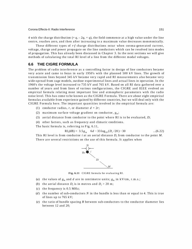
Corona Effects-II: Radio Interference 151
4 with the charge distribution (+ q, – 2q, + q), the field commence at a high value under the linecentre, reaches zero, and then after increasing to a maximum value decreases monotonically.
These different types of r-f charge distributions occur when corona-generated current,voltage, charge and power propagate on the line conductors which can be resolved into modesof propagation. This has already been discussed in Chapter 3. In the next sections we will givemethods of calculating the total RI level of a line from the different modal voltages.
6.6 THE CIGRE FORMULAThe problem of radio interference as a controlling factor in design of line conductors becamevery acute and came to focus in early 1950's with the planned 500 kV lines. The growth oftransmission lines beyond 345 kV became very rapid and RI measurements also became verywide-spread from cage models, outdoor experimental lines and actual lines in operation. In the1960's the voltage level increased to 735 kV and 765 kV. Based on all RI data gathered over anumber of years and from lines of various configurations, the CIGRE and IEEE evolved anempirical formula relating most important line and atmospheric parameters with the radionoise level. This has come to be known as the CIGRE Formula. There are about eight empiricalformulas available from experience gained by different countries, but we will deal only with theCIGRE Formula here. The important quantities involved in the empirical formula are:
(1) conductor radius, r, or diameter d = 2r;
(2) maximum surface voltage gradient on conductor, gm;
(3) aerial distance from conductor to the point where RI is to be evaluated, D;
(4) other factors, such as frequency and climatic conditions.The basic formula is, referring to Fig. 6.11,
RIi(dB) = 30)20/(log3365.3 10 −−+ im Ddg ...(6.22)This RI level is from conductor i at an aerial distance Di from conductor to the point M.There are several restrictions on the use of this formula. It applies when
Fig. 6.11 CIGRE formula for evaluating RI.
(a) the values of gm and d are in centimetre units; gm in kV/cm, r.m.s.;
(b) the aerial distance Di is in metres and Di > 20 m;
(c) the frequency is 0.5 MHz;
(d) the number of sub-conductors N in the bundle is less than or equal to 4. This is trueof lines up to 765 kV;
(e) the ratio of bundle spacing B between sub-conductors to the conductor diameter liesbetween 12 and 20;
2r
gm i
Di
M

152 Extra High Voltage AC Transmission Engineering
( f ) the weather condition is average fair weather;
( g ) the RI level has a dispersion of ± 6 dB.
Example 6.2. A 400-kV line has conductors in horizontal configuration at average heightH = 14 m and phase spacing S = 11 m, as shown in Figure 6.12. The conductors of each phaseare 2 × 0.0318 m diameter at B = 0.4572 m spacing. Calculate the RI level of each phase at adistance of 30 m from the outer phases at ground level at 0.5 MHz at 420 kV using the CIGREformula.
Fig. 6.12 Calculation of RI level of 400-kV line using CIGRE formula.
Solution. The first step is to calculate the maximum surface voltage gradient on thethree phases at 420 kV using the Mangoldt formula. Calculations give gmc = 17.3 kV/cm on thecentre phase and gm0 = 16.2 kV/cm on the two outer phases.
Aerial distances : D1 = 33 m, D2 = 43 m, D3 = 54 m.RI (1) = 3.5 × 16.2 + 6 × 3.18 – 30 – 33 log (33/20) = 38.6 dBRI (2) = 3.5 × 17.3 + 6 × 3.18 – 30 – 33 log (43/20) = 38.7 dBRI (3) = 3.5 × 16.2 + 6 × 3.18 – 30 – 33 log (54/20) = 31.6 dB.
6.6.1 Rules for Addition of RI Levels of 3-phases–S/C LineHaving calculated the RI level due to each phase at the measuring point, the rules for evaluatingthe total RI level of a 3-phase single-circuit line are as follows:
(a) If one of the RI levels is at least 3 dB higher than the rest, then this is the RI level ofthe line.
(b) Otherwise the RI level of line is
RI = (average of the two highest + 1.5) dB.
(c) At 1 MHz, the RI level is 6 dB lower.(d) For evaluating the RI level in rain, add 17 dB.
Example 6.3. In the previous example, calculate the RI level of the line at the measuringpoint at 0.5 MHz and 1 MHz in fair weather.
Solution. RI (3) is lower than the others by more than 3 dB.
∴ RIline = 21
(38.6 + 38.7) + 1.5 = 40.15 dB at 0.5 MHz and 34.15 dB at 1 MHz.
Example 6.4. In the above example, if the RI limit is given to be 40 dB at 1 MHz,calculate the width of right-of-way of the line corridor.
Solution. We observe that at 30 m from the outer phases, the RI level is 34.15 dB.Therefore, the value of 40 dB will be obtained at less than this distance. We will find the valueof d0 where RI = 40 dB at 1 MHz by trial and error.
33 43 54
1 2 3
30
14
11 11400 kV
M

Corona Effects-II: Radio Interference 153
For the outer phases, 3.5 × 16.2 + 6 × 3.18 – 30 = 45.78For the centre phase, 3.5 × 17.3 + 6 × 3.18 – 30 = 49.63.Assume d0 = 25, 20, 15 metres and calculate the RI level of line at 1 MHz.d0 D1 D2 D3 33 log 33 log 33 log RI(1) RI(2) RI(3)
(D1/20) (D2/20) (D3/20)25 28.7 38.6 49 5.15 9.43 12.83 40.6 40.2 3320 24.4 34 44.3 2.85 7.605 11.4 42.9 42 34.415 20.5 29.5 39.6 0.354 5.58 9.97 45.4 44 36
The resulting RI levels are
d0 = 25, RI = 41.9 at 0.5 MHz, 35.9 dB at 1 MHzd0 = 20, RI = 44 at 0.5 MHz, 38 dB at 1 MHzd0 = 15, RI = 46.2 at 0.5 MHz, 40.2 dB at 1 MHz∴ d0 = 15 metres at the edge of R-O-W, and the width of line corridor required is 2(d +s)
= 52 m. Since the CIGRE formula has a dispersion of ± 6 dB, further calculation may not benecessary. With this dispersion, a width of R-O-W giving 46 dB at 1 MHz at the edge of the linecorridor may be acceptable.
6.6.2 Rules for Addition of RI Levels for a D/C LineE.H.V. lines are mostly single-circuit (S/C) lines, but with the number of lines on the increaseand availability of land for the corridor increasingly difficult, double-circuit (D/C) and four-circuit 400-kV lines have been designed and commissioned. We will now discuss rules thatapply for adding RI levels of phase conductors in a D/C line only. The reader is recommendedfor advanced design papers and reports for 4-circuit RI problems since this depends entirely onthe possible combinations for the disposition of phases on the 4-circuit tower. (See SujathaSubhash, Ref. 18, under "Other Journals" in the Bibliography).
The first point to remember is to convert the RI levels in dB calculated by the CIGREFormula to microvolt/metre (µ V/m) by the relation.
).20/RI(/
dB10RI =µ mV ...(6.23)
On a D/C line, there are two phase-conductors belonging to each phase. Let RIA1 and RIA2be the RI values in µ V/m at any point M (measuring point) on ground (or at any convenientheight above it) due to phase A which can be evaluated individually by the CIGRE Formula indB and converted to µ V/m according to equation (6.23). Then the resulting RI value in µ V/mdue to the two conductors of phase A is give as the quadratic addition.
RIA = V/m,)RIRI( 2/122
21 µ+ AA ...(6.24a)
Similarly, RIB = .)RIRI(RIand)RIRI( 2/122
21
2/122
21 CCcBB +=+ ...(6.24b)
These are re-converted to dB values by the relation, RIdB = 20 log10 (RI), and are treatedas the contributions from the three phases. The rules for adding them to obtain the total RIlevel of line at the measuring point M will follow the rules as for a S/C line given before inSection 6.6.1.
The reason for quadratic addition is based upon the property that the pulses causing thenoise from any one phase are time-correlated from its two conductors so that energies orpowers are added arithmetically in the noise meter circuitry. It has been established fromsuitable experiments that if there are N identical noise sources which are correlated in time,

154 Extra High Voltage AC Transmission Engineering
that is, they occur on the same conductor or different conductors energized by the same voltage,then the resulting meter reading in mV /µ is for N non-identical but time-correlated sources,since this represents a quantity that is proportional to the energy or power (in a unit bandwidth).
RI(N) = ×N (RI due to each source acting individually).
∴ [RI(N)]2 = N × (RI)2, if all sources are identical.
or, = ),RI...RIRIRI( 223
22
21 N++++ ...(6.25)
Example 6.5. A D/C 400-kV line has the three conductors of one circuit at heights 13 m,23 m, and 33 m above ground, see Fig. 7.9. The horizontal spacings between conductors on thetower are 14 m , 16 m and 14 m between phases A1 – C2, B1 – B2, and C1 – A2, respectively. Thetwo-conductor bundles of each phase have conductors with diameters 3.18 cm each at a bundlespacing of 45.72 cm. At a point on ground 15 metres away from the line centre, evaluate thetotal RI level at 1 MHz in fair weather at 420 kV. (See p.181).
Solution. The Maxwell's Potential Coefficient matrix and its inverse for untransposedconfiguration are as follows.
[P] =
1 1 1 2 2 2
1
1
2
2
2
A B C A B C
BC
ABC
6.652, 1.718, 0.833, 0.678, 1.168, 1.573 A1
1.718, 6.290, 1.276, 0.772, 1.113, 1.168
0.833, 1.276, 5.720, 0.746, 0.772, 0.678
0.678, 0.772, 0.746, 5.720, 1.276, 0.833
1.168, 1.113, 0.772, 1.276, 6.290, 1.718
1.573, 1.168, 0.678, 0.833, 1.718, 6.652
[M] = [P]–1 =
170.9, – 36, – 10.7, – 6.56, – 15, – 28.3– 36, 181.7, – 30, – 10.7, – 15.5, – 15
–10.7, – 30, 187.4, – 15.8, – 10.7, – 6.56
– 6.56, – 10.7, – 15.8, 187.4, – 30, – 10.7
– 15, – 15.5, – 10.7, – 30, 181.7, – 36
– 28.3, – 15, – 6.56, – 10.7, – 36, 170.9
× 10–3
The voltage matrix is, with .kV3/420V =
[V] = ],120,120,0,120,120,0/[ °∠°−∠°∠°∠°−∠°∠ VVVVVVThe resulting bundle-charges cazn be expressed as
]2/[ 0eq π = ]][[ VM .
∴ =π 01 2/ eqA +°∠+°−∠+°∠ 120.120.0.[ 131211 VMVMVM
]120.120.0. 161514 °∠+°−∠+°∠ VMVMVM
= +°−∠++°∠+ 120).(0).[ 15121411 VMMVMM
].120).( 1613 °∠+ VMM

Corona Effects-II: Radio Interference 155
According to equation (4.38), its maximum value will be
01 2/ eqA π = 21613
21512
21411 )()()[( MMMMMMV +++++
))(())(( 1613151215121411 MMMMMMMM ++−++−2/1
14111613 )])(( MMMM ++−
= +−−+−× − 223 )1536()56.69.170[(103
420
)51)(56.69.170()3.287.10( 2 −−−−−2/1]34.164).39()39)(51( −−−−−
= .827.50∴ EA1 = (50.827/0.0318) (1 +0.0159/0.2286) = 1710 kV/m
= 17.1 kV/cm = EC2.Similar calculations yield
01 2/ eqB π = .42.512/ 02 =πeqB
giving EB1 = ,cm/kV3.17m/kV173006955.1)0318.0/42.51(2 ==×=BE
and EC1 = .kV/cm52.172 =AE
The aerial distances to the point on ground at 15 m from line centre are:
DA1 = ;m26.15)138(;m66.39)3322( 2/1222
2/122 =+==+ AD
DB1 = ;m24)237(;m53.32)2323( 2/1222
2/122 =+==+ BD
DC1 = ;m34)338(;m6.25)1322( 2/1222
2/122 =+==+ CDBy applying the CIGRE formula, the following dB values result which are converted to
mV/µ :
RA1 = ;m/36.90dB12.39)20/66.39(Log333018.361.175.3 Vµ==−−×+×RA2 = ;m/13.331dB4.503008.1952.175.3 Vµ=−−+×
ARI∴ = MHz.5.0atdB,71.50m/343)13.33136.90( 2/122 =µ=+ VSimilarly, RIB1 = ,m/8.135dB66.42 Vµ=and RIB2 = .m/4.224dB47 Vµ=
BRI∴ = .dB44.48m/22.264 =µV
RIC1 = ./m7.116dB34.41RIand,/m3.220dB86.46 2 VV C µ==µ=
CRI∴ = .dB48/m3.249 =µV
Finally, the total RI level of line is
RIT = average of the two highest + 1.5, dB
=21
(50.71 +48.44 +3) = 51.07 dB at 0.5 MHz
= 45.07 dB at 1 MHz.The same concept can be extended to any number of circuits on a tower.
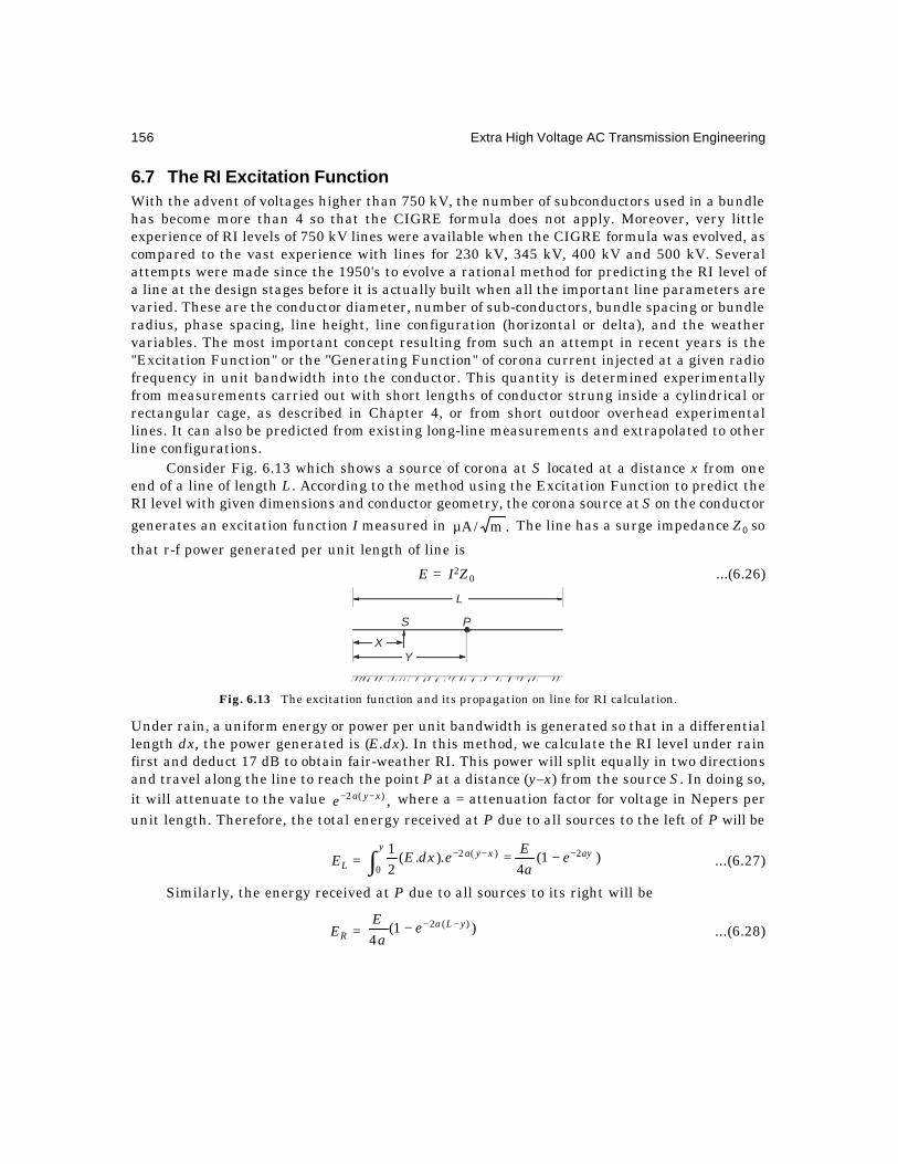
156 Extra High Voltage AC Transmission Engineering
6.7 The RI Excitation FunctionWith the advent of voltages higher than 750 kV, the number of subconductors used in a bundlehas become more than 4 so that the CIGRE formula does not apply. Moreover, very littleexperience of RI levels of 750 kV lines were available when the CIGRE formula was evolved, ascompared to the vast experience with lines for 230 kV, 345 kV, 400 kV and 500 kV. Severalattempts were made since the 1950's to evolve a rational method for predicting the RI level ofa line at the design stages before it is actually built when all the important line parameters arevaried. These are the conductor diameter, number of sub-conductors, bundle spacing or bundleradius, phase spacing, line height, line configuration (horizontal or delta), and the weathervariables. The most important concept resulting from such an attempt in recent years is the"Excitation Function" or the "Generating Function" of corona current injected at a given radiofrequency in unit bandwidth into the conductor. This quantity is determined experimentallyfrom measurements carried out with short lengths of conductor strung inside a cylindrical orrectangular cage, as described in Chapter 4, or from short outdoor overhead experimentallines. It can also be predicted from existing long-line measurements and extrapolated to otherline configurations.
Consider Fig. 6.13 which shows a source of corona at S located at a distance x from oneend of a line of length L. According to the method using the Excitation Function to predict theRI level with given dimensions and conductor geometry, the corona source at S on the conductor
generates an excitation function I measured in .m/Aµ The line has a surge impedance Z0 so
that r-f power generated per unit length of line is
E = I2Z0 ...(6.26)
Fig. 6.13 The excitation function and its propagation on line for RI calculation.
Under rain, a uniform energy or power per unit bandwidth is generated so that in a differentiallength dx, the power generated is (E.dx). In this method, we calculate the RI level under rainfirst and deduct 17 dB to obtain fair-weather RI. This power will split equally in two directionsand travel along the line to reach the point P at a distance (y–x) from the source S. In doing so,it will attenuate to the value ,)(2 xyae −− where a = attenuation factor for voltage in Nepers perunit length. Therefore, the total energy received at P due to all sources to the left of P will be
EL = ∫ −−− −=y
ayxya ea
EedxE0
2)(2 )1(4
)..(21
...(6.27)
Similarly, the energy received at P due to all sources to its right will be
ER = )1(4
)(2 yLaea
E −−− ...(6.28)
L
XY
S P

Corona Effects-II: Radio Interference 157
For a line of finite length, repeated reflections occur from the ends, but for a very longline these are not of consequence. Also, unless the point P is located very close to the ends, theexponential terms can be neglected. Therefore, the total r-f energy received at P will be
Ep = E/2a ...(6.29)which shows that all points on a long line receive the same r-f energy when the corona
generation is uniform.
Example 6.6. For attenuation factors of 6, 1 and 0.17 dB/km, calculate the energyreceived at point P in terms of energy generated per unit length.
Solution. The conversion factor from dB to Nepers is 8.7. Thus, a = 0.69 N/km for 6 dB/km, 0.115 N/km for 1 dB/km, and 0.019 N/km for 0.17 dB/km.
PE∴ = E/2a = 0.7246 × energy generated per km for a = 6 dB/km
EP = 4.348 × energy generated per km for a = 1 dB/kmand EP = 25.575 × energy generated per km for a = 0.17 dB/km.Associated with the current injected into the conductor per unit length, there is a voltage
to ground which is known as the Radio Influence Voltage (RIV). Then,EP = E/2a = (RIV)2/Z0 ...(6.30)
But E = I2Z0 so that (RIV) = aIZ 2/0 ...(6.31)
The ground level field depends upon the conductor charge per unit length and the fieldfactor, as shown in Section 6.5. If the capacitance of line per unit length is C, the charge is
q = C(RIV) = aICZ 2/0 ...(6.32)
However, for an overhead line, the velocity of propagation, capacitance, and surgeimpedance are related by
v = 1/C Z0 ...(6.33)
∴ q = avI 2/ ...(6.34)
Since the charge is found in terms of the excitation function, velocity, and attenuationfactor, the resulting RI level of line is
RI = ]2/[FactorField 00
aHveIFHe
qπ=×
π ...(6.35)
Thus, the quantities involved in estimating the RI level of a line at a specific distance dfrom the line centre (or a corresponding distance from the outer phase) are the following:
(a) the field factor F which is a function of the line geometry (H,s,d);
(b) the line height H;
(c) the velocity of propagation v;
(d) the attenuation factor, a; and
(e) the injected current or the excitation function, I.The velocity and attenuation factors are known either by performing suitable experiments
on existing lines, or calculated if possible. The field factor is also calculated. However, theexcitation function I can only be determined for the conductor under consideration from small-scale experiments using artificial rain apparatus and cages or outdoor overhead lines.
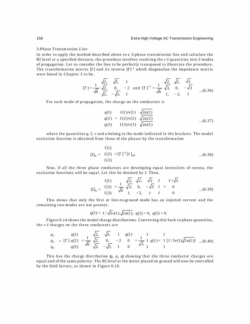
158 Extra High Voltage AC Transmission Engineering
3-Phase Transmission LineIn order to apply the method described above to a 3-phase transmission line and calculate theRI level at a specified distance, the procedure involves resolving the r-f quantities into 3 modesof progagation. Let us consider the line to be perfectly transposed to illustrate the procedure.The transformation matrix [T] and its inverse [T]–1 which diagonalize the impedance matrixwere found in Chapter 3 to be.
−−=
−−= −
1,2,1
3,0,3
2,2,2
6
1][and
1,3,2
2,0,2
1,3,2
6
1][ 1TT
...(6.36)
For each mode of propagation, the charge on the conductors is
=
)3(2)3(/)3(
)2(2)2(/)2(
)1(2)1(/)1(
)3(
)2(
)1(
avIavIavI
qqq
...(6.37)
where the quantities q, I, v and a belong to the mode indicated in the brackets. The modalexcitation function is obtained from those of the phases by the transformation
[I]m = phITIII
][][
)3(
)2(
)1(1−=
...(6.38)
Now, if all the three phase conductors are developing equal intensities of corona, theexcitation functions will be equal. Let this be denoted by I. Then.
[I]m =
=
−−=
0
0
3/
1,2,1
3,0,3
2,2,2
6
1
)3(
)2(
)1( I
III
III
...(6.39)
This shows that only the first or line-to-ground mode has an injected current and theremaining two modes are not present.
∴ q(1) = .0)3(,0)2(,)1(2).1(3/ == qqavI
Figure 6.14 shows the modal charge distributions. Converting this back to phase quantities,the r-f charges on the three conductors are
3
2
1
qqq
= ])1(2)1(3/[
1
1
1
)1(
1
1
1
3
1
0
0
)1(
1,3,2
2,0,2
1,3,2
6
1
)3(
)2(
)1(
][ avIqq
qqq
T
=
=
−−=
...(6.40)
This has the charge distribution (q, q, q) showing that the three conductor charges areequal and of the same polarity. The RI level at the meter placed on ground will now be controlledby the field factors, as shown in Figure 6.10.

Corona Effects-II: Radio Interference 159
Fig. 6.14 Modal charge distributions on a fully-transposed 3-phase ac line.
Thus, RI1 = 22 /)(1
1
HsdHeq
o −+π
RI2 = 20 )/(1
1
HdHeq
+π ...(6.41)
and RI3 = 220 /)(1
1
HsdHeq
++π
The addition rule according to the CIGRE formula can now be applied to these three RIlevels and the RI level of the line calculated. The quantities to be ascertained are I, v and afrom measurements. The velocity and attenuation factor pertain to this mode of excitationwhile the excitation function applies to the conductor usually performed in a cage arrangementin single-phase configuration at the correct surface voltage gradient that exists on the overheadline.Bipolar DC Line
It is interesting to observe the properties of modal excitation functions on a bipolar dc lineand compare these with a perfectly transposed 3-phase ac line.
In Sections 6.1 and 6.2 it was mentioned that radio noise is almost entirely caused bypositive corona pulses so that on a bipolar dc line, only the positive-polarity conductor developsmeasurable r-f energy. Thus, the excitation functions will be .]0,[][ tp II += The transformation
matrix and its inverse used for diagonalizing the impedance of a bipolar dc line are
[T] =
−
=−
1,1
1,1
2
1][ 1T ...(6.42)
The excitation function in the two modes will be
)2(
)1(
II
= )2/(1
1][][ 1
+−
= IIT p ...(6.43)
This shows that both modes contain equal amounts of injected current, while we observedthat on a perfectly-transposed 3-phase ac line there was no energy or excitation in two of themodes. All the energy was retained in the first or line-to-ground or the homopolar mode ofpropagation. This is the essential difference between the two lines.
The corresponding charge distributions in the two modes are
[q]m =
=
=
)2().2(
)1().1(
)2(2)2(/)2(
)1(2)1(/)1()2(
)1(
IKIK
avI
avIqq
… (6.44)
q(1) q(1) q(1)
Ist Mode IInd Mode IIIrd Mode
q(3) = 0q(2) = 0q v(1) = I / 3 (I) 2 (I)a

160 Extra High Voltage AC Transmission Engineering
Figure 6.15 depicts the modal charge distributions. Converting this back to the chargesresiding on the poles by multiplying [q]m by [T], there results.
Fig. 6.15 Modal charge distributions on a bipolar dc line.
[q] = mqTqq
]][[=
−
+
=
−++
)2()1(
)2()1(
2 KKKKI
...(6.45)
We observe that even though the negative pole is not developing any r-f energy it has acharge due to mutual coupling from the positive pole. The RI level at ground level can becalculated at two representative points M1, M2 at the same lateral distance d from the linecentre with M1 closer to the positive pole and M2 nearer the negative pole, Fig. 6.16.
Fig. 6.16 Conductor r-f charge distribution on bipolar dc line after transforming modal charges by [T].
At M1
Due to positive conductor,
)(RI 1M+ = 220
220 /)2/(1
)2()1(2/)2/(1
1
HPd
KKHe
I
HPdHeq
−+
+π
=−+π
++...(6.46)
Due to the negative conductor
)(RI 1M− = 220 /)2/(1
)2()1(2 HPd
KKHe
I
++
−π
+...(6.47)
Similarly at M2
)(RI 2M+ = 220 /)2/(1
)2()1(2 HPd
KKHe
I
++
+π
+...(6.48)
)(RI 2M− = 220 /)2/(1
)2()1(2 HPd
KKHe
I
−+
−π
+...(6.49)
q(1) = I/ 2 (1) 2 (1)v a+ q I v(2) = / 2 (2) 2 (2)a+
q(1) q(1) q(2) q(2)
q+ q–
M1 M2
P
d d
H

Corona Effects-II: Radio Interference 161
where )1(K = )2(2)2(/1)2(and)1(2)1(/1 avKav = ...(6.50)
In general, the velocities in the two modes will be different with v (1) being about 80%light velocity since it involves ground return and v(2) equal to light velocity. The attenuationfactors a(1) and a(2) will also be different with a(1) equal to about 6 dB/km (0.69 Neper/km) anda(2) equal to about 1 dB/km (0.115 Neper/km).
Procedure for Obtaining Excitation Function from CIGRE FormulaSince the procedure for calculating RI level from the excitation function parallels the empiricalformula given by the CIGRE, we will now examine the relation between the expressions givenin equations (6.40) for the charge and the resulting RI with (6.22). For the charge given in(6.40), the RI level at ground will be
RI = 220 /1
11
23 HdHeav
I
+π ...(6.51)
The corresponding decibel value is
RIdB = ]/)[(Log20)23(Log20)/(Log20 2221010010 HHdaHveI +−π− ...(6.52)
The first term aHveIg 0/= has dimension volt/metre and therefore corresponds to thevoltage gradient in the CIGRE formula.
===
×××
metreVolt
metre-FaradCoulomb
metre-FaradSec-Amp
mm
NepermF
sm
)m/Amp(
The other quantities in equation (6.52) are dimensionless.
∴ RIdB = )/(log405.22Log20 221010 HHdg +−− ...(6.53)
The CIGRE formula is
RIdB = )20/(Log3330125.3 22 Hdrgm +−−− ...(6.54)
By calculating the RI level for a given conductor using the CIGRE formula and equating itto equation (6.53), the value of g can be determined and thereby the excitation function I, asshown by an example.
Example 6.7 In example 6.2, the RI level at 30 m from outer phase due to the centrephase was calculated as 38.7 dB when H = 14 m, r = 1.59 cm, gm = 17.3 kV/cm and d = 41m. (a)Calculate the value of g in equation (6.53) by equating (6.54) with it. (b) Takingv = 2.5 × 10⁸ m/s and a =0.69 × 10⁻³ Neper/m, calculate the excitation function and its dB
value above 1 .m/Aµ
Solution. 38.7 = 1.42)(Log2014/1441Log405.22)(Log20 22 −=
+−− gg
(a) ∴ g = antilog 4.04 = 1.0965 ×10⁴ volt/metre = 10.965 kV/m
(b) I = .m/A984.81069.01410842.8105.2100965.1 312840 µ=×××××××= −−aHgve
IdB = .m/A1abovedB07.19984.8Log20 10 µ=Thus, the RI level is 19.63 dB higher than the dB value of the excitation function. The
decibel adder to convert the excitation function to the RI level is therefore 19.63 dB for thisexample.
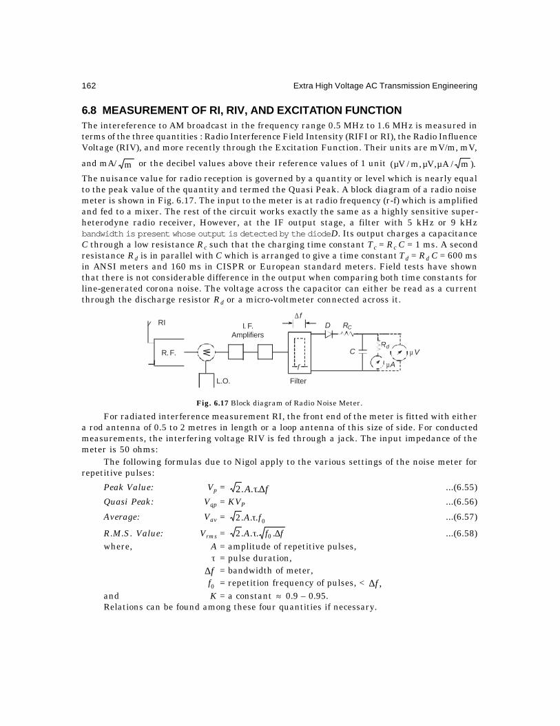
162 Extra High Voltage AC Transmission Engineering
6.8 MEASUREMENT OF RI, RIV, AND EXCITATION FUNCTIONThe intereference to AM broadcast in the frequency range 0.5 MHz to 1.6 MHz is measured interms of the three quantities : Radio Interference Field Intensity (RIFI or RI), the Radio InfluenceVoltage (RIV), and more recently through the Excitation Function. Their units are mV/m, mV,
and mA/ m or the decibel values above their reference values of 1 unit ).m/A,V,m/V( µµµ
The nuisance value for radio reception is governed by a quantity or level which is nearly equalto the peak value of the quantity and termed the Quasi Peak. A block diagram of a radio noisemeter is shown in Fig. 6.17. The input to the meter is at radio frequency (r-f) which is amplifiedand fed to a mixer. The rest of the circuit works exactly the same as a highly sensitive super-heterodyne radio receiver, However, at the IF output stage, a filter with 5 kHz or 9 kHzbandwidth is present whose output is detected by the diode D. Its output charges a capacitanceC through a low resistance Rc such that the charging time constant Tc = Rc C = 1 ms. A secondresistance Rd is in parallel with C which is arranged to give a time constant Td = Rd C = 600 msin ANSI meters and 160 ms in CISPR or European standard meters. Field tests have shownthat there is not considerable difference in the output when comparing both time constants forline-generated corona noise. The voltage across the capacitor can either be read as a currentthrough the discharge resistor Rd or a micro-voltmeter connected across it.
Fig. 6.17 Block diagram of Radio Noise Meter.
For radiated interference measurement RI, the front end of the meter is fitted with eithera rod antenna of 0.5 to 2 metres in length or a loop antenna of this size of side. For conductedmeasurements, the interfering voltage RIV is fed through a jack. The input impedance of themeter is 50 ohms:
The following formulas due to Nigol apply to the various settings of the noise meter forrepetitive pulses:
Peak Value: Vp = fA ∆τ...2 ...(6.55)
Quasi Peak: Vqp = KVP ...(6.56)
Average: Vav = 0...2 fA τ ...(6.57)
R.M.S. Value: Vrms = ffA ∆τ ....2 0 ...(6.58)where, A = amplitude of repetitive pulses,
τ = pulse duration,f∆ = bandwidth of meter,
0f = repetition frequency of pulses, < ,f∆and K = a constant ≈ 0.9 – 0.95.Relations can be found among these four quantities if necessary.
R. F.
∆ f
µA
µ V
D RC
RdC
I. F.Amplifiers
RI
L.O. Filter
f
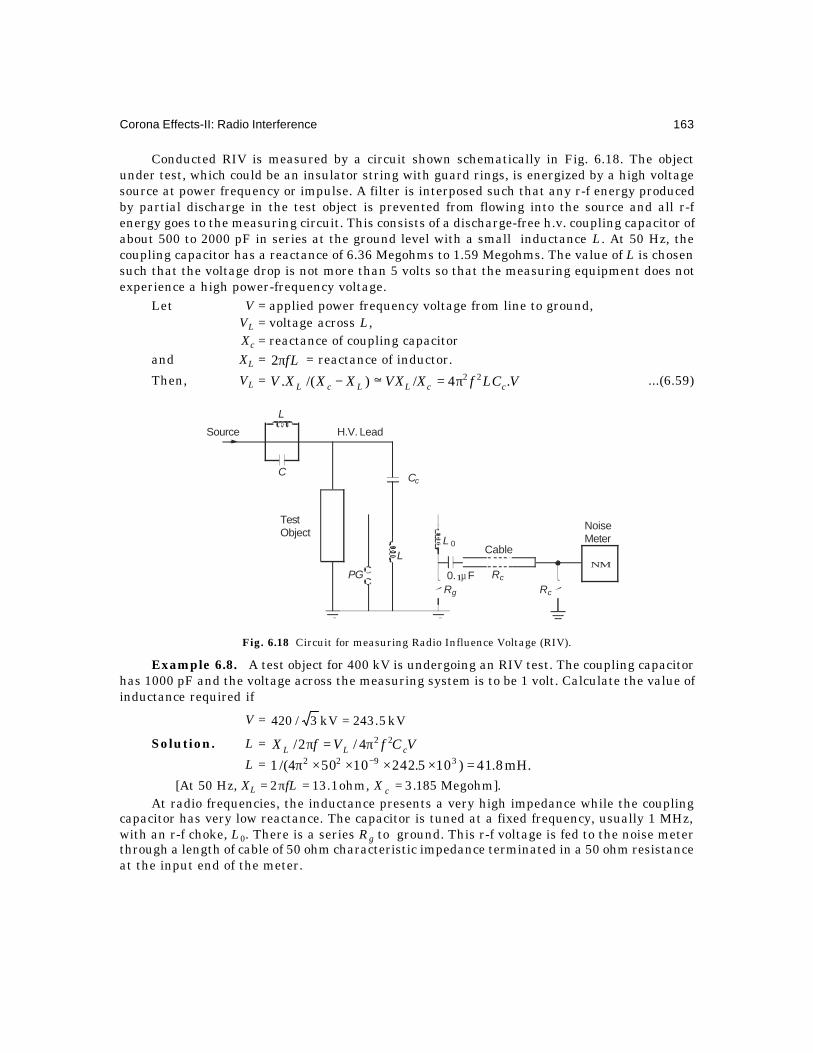
Corona Effects-II: Radio Interference 163
Conducted RIV is measured by a circuit shown schematically in Fig. 6.18. The objectunder test, which could be an insulator string with guard rings, is energized by a high voltagesource at power frequency or impulse. A filter is interposed such that any r-f energy producedby partial discharge in the test object is prevented from flowing into the source and all r-fenergy goes to the measuring circuit. This consists of a discharge-free h.v. coupling capacitor ofabout 500 to 2000 pF in series at the ground level with a small inductance L. At 50 Hz, thecoupling capacitor has a reactance of 6.36 Megohms to 1.59 Megohms. The value of L is chosensuch that the voltage drop is not more than 5 volts so that the measuring equipment does notexperience a high power-frequency voltage.
Let V = applied power frequency voltage from line to ground,VL = voltage across L,Xc = reactance of coupling capacitor
and XL = fLπ2 = reactance of inductor.
Then, VL = VLCfXVXXXXV ccLLcL .4/~)/(. 22π=−− ...(6.59)
Fig. 6.18 Circuit for measuring Radio Influence Voltage (RIV).
Example 6.8. A test object for 400 kV is undergoing an RIV test. The coupling capacitorhas 1000 pF and the voltage across the measuring system is to be 1 volt. Calculate the value ofinductance required if
V = kV5.243kV3/420 =
Solution. L = VCfVfX cLL224/2/ π=π
L = .mH8.41)105.24210504/(1 3922 =××××π −
[At 50 Hz, XL = ].Megohm185.3,ohm1.132 ==π cXfLAt radio frequencies, the inductance presents a very high impedance while the coupling
capacitor has very low reactance. The capacitor is tuned at a fixed frequency, usually 1 MHz,with an r-f choke, L0. There is a series Rg to ground. This r-f voltage is fed to the noise meterthrough a length of cable of 50 ohm characteristic impedance terminated in a 50 ohm resistanceat the input end of the meter.
Source
L
C
H.V. Lead
NoiseMeter
Cable
RcPG
TestObject
RcRg
Cc
L 0
L
0. F1µNM

164 Extra High Voltage AC Transmission Engineering
The value of L0 is obtained from the equation.
f = cc CfLCL 2200 4/1or2/1 π=π ...(6.60)
where f = measuring frequency.
Example 6.9. In the above example with Cc = 1000 pF, calculate(a) the value of L0 to tune the circuit to 1 MHz,
(b) the reactance of L = 41.8 mH at 1 MHz and(c) that of the coupling capacitor Cc. Check with reactance of L0.Solution.
(a) L0 = .H33.2510104/1 9122 µ=××π −
(b) XL = .kilohms64.262108.41102 36 =×××π −
(c) Xc = .ohms15910102/1 96 =××π −
XL0 = .ohms1591033.25102 66 =×××π −
The r-f voltage developed across Rg is fed to the noise meter. Since transmission lineshave a characteristic impedance in the range 300 to 600 ohms, standard specifications stipulatedthat the r-f voltage must be measured across 600 ohms. Thus, Rg is in the neighbourhood of 600ohms. However, it was obvious that this could not be done since the presence of cable willlower the impedance to ground. In earlier days of RIV measurement at lower voltages (230 kVequipment) the noise meter was directly connected across Rg and its input end was open. Theoperator sat right underneath the pedestal supporting the coupling capacitor in order to readthe meter or used a pair of binoculars from a distance. But with increase in test voltage, theneed for maintaining a safe distance necessitates a cable of 10m to 20m. With its surgeimpedance Rc conected across Rg, which has a higher value, the combined parallel impedanceis lower than Rc. No coaxial cables are manufactured for high surge impedance, so that standardspecifications allow RIV to be measured across 150 ohm resistance made up of Rg and Rc inparallel. It is clear that the measuring cable must have Rc greater than 150 ohms. The highestimpedance cable has Rc = 175 ohms on the market. The value of Rg can be selected such that
)/( gcgc RRRR + = 150 ohms
giving Rg = 150 Rc/(Rc –150) ...(6.61)For Rc = 175 ohms, Rg = 6 Rc = 1050 ohms.The meter reading is then multiplied by a factor of 4 in order to give the RIV measured
across 600 ohms, or by a factor of 2 for 300 ohms surge impedance.
6.9 MEASUREMENT OF EXCITATION FUNCTIONThe corona generating function or the excitation function caused by injected current at radiofrequencies from a corona discharge is measured on short lengths of conductor strung inside"cages" as discussed earlier. The design of cages has been covered in great detail in Chapter 4,Some examples of measuring radio noise and injected current are shown in Fig. 6.19. In everycase the measured quantity is RIV at a fixed frequency and the excitation function calculated asdescribed later. The filter provides an attenuation of at least 25 dB so that the RI current issolely due to corona on conductor. The conductor is terminated in a capacitance Cc at one endin series with resistances R1 and Rc, while the other end is left open. The conductor is strungwith strain insulator at both ends which can be considered to offer a very high impedance at 1

Corona Effects-II: Radio Interference 165
MHz so that there is an open-termination. But this must be checked experimentally in situ.The coupling capacitor has negligible reactance at r-f so that the termination at the measuringend is nearly equal to (R1 + Rc), where Rc = surge impedance of the cable to the noise meter.The resistance Rc is also equal to the input impedance of the noise meter.
Fig. 6.19 Cage setups for measuring excitation function with measuring circuit.
The excitation function is calculated as follows:
Let J = RI current injected in ,m/Aµ
C = capacitance of conductor in cage, Farad/metre,
R = outer radius of cage,req = equivalent radius of bundle.
Then, the excitation function is
I = m/A,/.2 0 µπ CJe ...(6.62)
The injected current in terms of measured RIV is
J = GRRRR mcmc /)RIV)((2 + ...(6.63)
where =+ )/( mcmc RRRR resistance of Rc and meter in parallel,
RIV = measured noise reading on meter in ,Vµ
and G = an amplification factor caused by addition of the uniformly distributedr-f currents generated on the conductor.
The test is normally carried out under rain conditions from artificial rain apparatus sothat corona is generated uniformly along the conductor. For a line terminated at one end in itssurge impedance with the other end open, the amplification factor is, for a conductor length L.
G =
ππ
+=
π∫ vfL
fvLdxx
vfL 4
sin82
.2
cos0
2...(6.64)
where v = velocity of propagationand f = frequency of measurement.Since Rc = Rm, there results
I = .m/A),RIV.(42 0 µ
πGRC
e
c...(6.65)
CONDUCTOR
CAGE
Source
NM
Cc
R
( )a
F
NMCoax Cable
Source
Filter
CONDUCTORL
CAGE
Cc
R1
Rc
( )b

166 Extra High Voltage AC Transmission Engineering
This value of excitation function has been used in Section 6.7 for evaluating the RI level ofa long line.
6.10 DESIGN OF FILTERWhen corona is generated on the bundle-conductor inside the cage or on a test object duringRIV measurements, the energy in the pulses will be divided between the measuring circuit andthe source transformer. The transformer can be assumed to offer a pure capacitive reactanceconsisting of the h.v. bushing and the winding inductance at the frequency of r-f measurement,usually 1 MHz. Fig. 6.20 shows a simple R-L filter, for which the attenuation factor is
A = |Vi/V0| = 2/122222 ])1[( tftf CRwCLw +− ...(6.66)
This is obtained by simple voltage division which is
Vi /V0 = )]1/(/[)]1/()[( 22ttttttff CLwjwLCLwjwLLjwR −−++ ...(6.67)
where =π= tCfw ,2 transformer capacitance, L t = transformer inductance, andRf, Lf = filter resistance and inductance.
Let the upper and lower frequencies of measurement be f2 and f1, and the desiredattenuations A2 and A1. The decibel values are
D2 = .log20andlog20 1101210 ADA =Then the following equations hold from which we can calculate the products
.and tftf CRYCLX == When the transformer capacitance is known, the values of filter elementsare fixed.
22
222
222 )1( AYwXw =+− ...(6.68)
21
221
221 )1( AYwXw =+− ...(6.69)
Then, 21
21
22
22
221
22 /)1(/)1()( wAwAXww −−−=− ...(6.70)
Fig. 6.20 Line filter for blocking corona energy from entering source transformer.
and 22
222
22
2 /])1([ wXwAY −−= ...(6.71a)
or, 21
221
21
2 /])1([ wXwAY −−= ...(6.71b)
The Q of the filter at any frequency is,
./2/2 YfXRLfQ ff π=π= ...(6.72)
V0
CORONA ONCONDUCTOR
MC V0CtLt
Lf Rf

Corona Effects-II: Radio Interference 167
Example 6.10. Design a filter to give 40 dB attenuation at 1 MHz and 25 dB at 0.4 MHz.Calculate Q of filter at 1 MHz.
Solution. Let w2 = ,100,104.02,102 26
16 =××π=×π Aw
A1 = .78.1710 25.1 =12221222222122 1016.04/)178.17(104/)1100()4.01(104 ××π−−×π−=−×π∴ X
This gives X = 121076.5 −×=tfCL
Then, Y2 = 1222121222 104/])1076.51041(100[ ×π×××π−− −
giving Y = .101.16 6tfCR=× −
Q = .MHz1at248.2/2/2 =π=π YXfRLf ff
Example 6.11. The limiting frequencies for AM broadcast are 0.5 MHz and 1.6 MHz.Design filter elements Lf and Rf and find Q at 1 MHz for giving 40 dB at 1.6 MHz and 25 dB at0.5 MHz.
Solution. Using equations (6.68) to (6.71), there result
X = 612 10222.5and10852.0 −− ×==×= tftf CRYCL
Q = .MHz1at025.1
If the transformer capacitance is 1000 pF = 10–9 Farad, the values are Lf = 0.852 mH andRf = 5.222 kilohms.
The most important point to observe is that even though the filter elements are in serieswith the source transformer and conductor in the cage at the high voltage, they must bedesigned for the full working voltage. This is a very expensive item in the experimental set-up.
6.11 TELEVISION INTERFERENCE (TVI)Television (TV) and Frequency Modulation (FM) broadcast and reception normally coverfrequencies in the range 25 to 100 MHz. The audio portion of TV is frequency modulated and isgenerally insensitive to noise generated by power lines, equipment and hardware at high voltagegradients, and sparks. This is also true of video synchronizing circuits. The only part sensitiveto noise is the AM carrier-signal processing circuit which is disturbed during the sweep of theelectron beam across the TV picture-tube screen. We will briefly discuss the effects this has onthe quality of TV reception and the types of noise which affect it. No effort is made to describetechnical aspects of TV transmission and reception here and the reader should consult literatureof excellent quality and vast extent existing on TV engineering.
Interference to TV reception from e.h.v. power lines came into focus in late 1960's andearly 1970's with the energization of 500 kV lines, in a manner similar to audible noise. At thattime the primary cause of TVI was recognized as corona discharges from water drops on thesingle and bundled conductors, the former yielding higher disturbance than the latter. Thedisturbance on the TV screen was observed as bands or streaks drifting across it. Prior to thisobservation, residential dwellings were located at least 60 metres from the centre of a powerline which was based on RI limitations, but resulted in TVI during heavy rain conditions. Thenoise level was 3 µV/m (9.54 dB) at 75 MHz in fair weather but increased to 30 µV/m (29.54 dB)in foul weather when at the same time the RI level was measured as 1800 µV/m (65.1 dB).

168 Extra High Voltage AC Transmission Engineering
Wet-snow conditions gave maximum TVI. These observations prompted serious attention to begiven to TVI and the nature of discharges emanating from e.h.v. power lines causing thisinterference. The problem of interference to B & W and colour TV had, of course, been alreadyunder investigation from man-made sources since a long time prior to this.
It was soon recognized that allowable noise should be set 5 µV/m(14 dB) where the TVsignal had a strength of 40 dB higher (100 : 1 ratio for signal to noise). For satisfactory reception,the signal strength is specified as a minimum of 225 µV/m(47 dB) which is permitted in ruralareas and much higher in urban areas close to TV transmitters. In foul weather, measurednoise at 75 MHz can be 5 µV/m(14 dB) even at 150 metres from the line which is consideredsatisfactory for TV reception in rural areas where the signal strength can be as low as 225 µV/m. At 60 metres from the line, the noise is about 30 µV/m (29.54 dB) which would then require69.54 dB (3000 µV/m). A measured value of 2500 µV/m(68 dB) was seen to give tolerably goodreception. In fair weather, these limits exist and line noise is observed not to disturb TVreception even under the line,. Thus TVI is of great concern only in foul weather from a line,but as will be explained later, micro-discharges from line hardware can be a nuisance even infair weather. These must be located and corrected by proper maintenance if complaints are notto be forthcoming. We shall now briefly enumerate the types of discharges from an e.h.v. linethat cause TVI and the types of possible TVI observed in practice. With the enormous popularitythat TV has achieved in recent years even in rural India, the problem of TVI is as important asin other countries where TV has been used in farming communities not only for entertainmentbut also for gathering information for their everyday life, so that TVI should be treated seriouslyby regulating bodies and environmentalists.
There are three types of noise sources from an e.h.v. power transmission line which areof concern. These are:
(a) Ultra corona on thin wires or slivers or sharp edges and points;
(b) Corona on conductors;(c) Sparking from cracked insulators, and across small gaps such as loose connections
between line hardware components, which are especially troublesome during windconditions.
Ultra corona is a phenomenon that is recognized to occur at voltage gradients much inexcess of normal corona inception and is a variety of glow corona. Normally, glow corona of theluminous type does not exhibit pulse-type property but as the voltage gradient exceeds22 kV/cm, r.m.s., pulse-type discharge commences during the negative half-cycle of power-frequency excitation. The resulting noise is very similar to that generated by corona on a wetconductor during the negative half-cycle. It was mentioned in Sections 6.1 and 6.2 that this wasnot of concern for Radio Interference because these amplitudes and time durations of negativepulses when processed through the 5 kHz bandwidth of the Quasi-Peak circuit of a Radio Noisemeter resulted in insignificant level of noise as compared to positive corona noise. However,the frequency spectrum of negative pulses exhibits a more constant or flat type than that ofpositive pulses and this is serious from TVI point of view. Figure 6.21 shows relative amplitudeplots of the frequency spectra of four types of discharges from lines, where it can be observedthat positive corona noise decreases at the rate of 35 dB per decade increase in frequency whilenegative noise shows a decrease of only 20 dB decrease per decade. The gap-type noise is nearlyflat upto 100 MHz which is of concern for TVI.
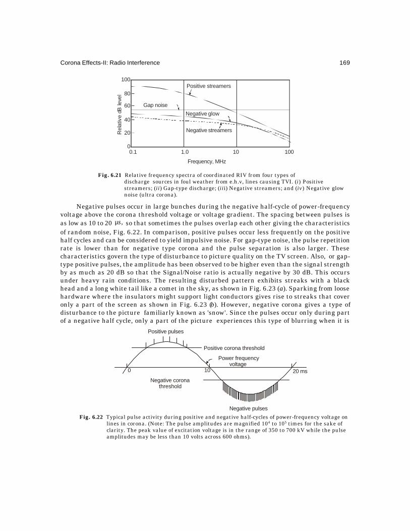
Corona Effects-II: Radio Interference 169
Fig. 6.21 Relative frequency spectra of coordinated RIV from four types of discharge sources in foul weather from e.h.v, lines causing TVI. (i) Positive streamers; (ii) Gap-type discharge; (iii) Negative streamers; and (iv) Negative glow noise (ultra corona).
Negative pulses occur in large bunches during the negative half-cycle of power-frequencyvoltage above the corona threshold voltage or voltage gradient. The spacing between pulses isas low as 10 to 20 ,sµ so that sometimes the pulses overlap each other giving the characteristicsof random noise, Fig. 6.22. In comparison, positive pulses occur less frequently on the positivehalf cycles and can be considered to yield impulsive noise. For gap-type noise, the pulse repetitionrate is lower than for negative type corona and the pulse separation is also larger. Thesecharacteristics govern the type of disturbance to picture quality on the TV screen. Also, or gap-type positive pulses, the amplitude has been observed to be higher even than the signal strengthby as much as 20 dB so that the Signal/Noise ratio is actually negative by 30 dB. This occursunder heavy rain conditions. The resulting disturbed pattern exhibits streaks with a blackhead and a long white tail like a comet in the sky, as shown in Fig. 6.23 (a). Sparking from loosehardware where the insulators might support light conductors gives rise to streaks that coveronly a part of the screen as shown in Fig. 6.23 (b). However, negative corona gives a type ofdisturbance to the picture familiarly known as 'snow'. Since the pulses occur only during partof a negative half cycle, only a part of the picture experiences this type of blurring when it is
Fig. 6.22 Typical pulse activity during positive and negative half-cycles of power-frequency voltage onlines in corona. (Note: The pulse amplitudes are magnified 104 to 105 times for the sake ofclarity. The peak value of excitation voltage is in the range of 350 to 700 kV while the pulseamplitudes may be less than 10 volts across 600 ohms).
Positive pulses
Positive corona threshold
Power frequencyvoltage
Negative coronathreshold
Negative pulses
20 ms0 10
0.1 1.0 10 100
100
80
60
40
20
0
Rel
ativ
edB
leve
l
Frequency, MHz
Negative streamers
Negative glow
Positive streamers
Gap noise

170 Extra High Voltage AC Transmission Engineering
Fig. 6.23 Typical patterns of Television Interference (TVI),(a) Due to positive gap-type noise. Noise level is higher than carrier signal strength
by about 20 dB.(b) Due to sparking at loose hardware.
realized that a normal TV screen has 525 lines sweeping across it in two frames at nearly 50times a second. This corresponds nearly to power-frequency voltage also. Therefore, negativepulses occurring during only a part of a power-frequency cycle will cause blurring at the middleof the screen from a single phase and nearly completely from the three phases. Observationsmade by G.W. Juette at the E.H.V. Project have revealed the following types of behaviour forTVI, (Ref. 115, IEEE in Bibliography):
(a) When S/N ratio is 0 dB, about 50% of screen has dense white bands from a single-phase noise source;
(b) If the S/N ratio is more favourable, at 20 dB, the band separates into balck and whitespots;
(c) At S/N ratio of 20 dB, the spots become smaller and show a larger separation;
(d) At 30 dB S/N ratio, the separation is even more and main picture assumes morebrightness but is not yet clear;
(e) At 40 dB, very few spots are visible and there is no snow. This appears to be thethreshold for noise nuisance;
( f ) At 50 dB, the picture is very clear and noise effect is not visible.Works of Giao Trinh and Jordan, and recently by the team of Arai, Miguchi and
Janischewskyj have emphasized the need for careful investigation into the frequency spectrumof different modes of corona and transition from streamer to spark discharges in order toassess their effect on TV interference so that remedial measures may be taken. (See References114 and 119, IEEE in Bibliography).
Review Questions and Problems
1. Describe the mechanism of formation of a positive corona pulse train.2. The positive and negative corona pulses can be assumed to be square pulses of
amplitudes 100 mA and 10 mA respectively. Their widths are 200 ns and 100 nsrespectively. Their repetition rates are 1000 pps and 10,000 pps. The bandwidth of afilter is 5 kHz. Using equation (6.15) calculate the ratio of output of the filter for thetwo pulse trains at a tuned frequency f0 = 1 MHz.
( )a ( )b

Corona Effects-II: Radio Interference 171
3. At a town near which a proposed e.h.v. line will run, the measured radio-station fieldstrengths are as follows:
Frequency ofStation 0.5 0.75 0.9 1.0 1.1 1.2 1.3 1.4 1.5 MHz
Received SignalStrength 50 60 75 70 65 52 80 75 60 dB
Take the corona noise from a line to vary as f–1.5, and the minimum S/N ratio to be 22dB. If the station at 1 MHz is to be received with this quality of reception, determinewhich of the stations will have a S/N ratio lower than the minimum allowable S/Nratio of 22 dB.
4. Calculate and plot the field factors for the 3 modes of propagation for a line with H =15 m, S = 12 m as the distance from the line centre is varied from 0 to 3 H.
5. The heights of conductors of a bipolar dc line are H = 18 m and the pole spacing P =12 m. Calculate and plot the field factors for this line for the two modes of propagationas the distance d from line centre is varied from 0 to 3 H.
6. A 750-kV line in horizontal configuration has H = 18 m and phase spacing S = 15 m.The conductors are 4 × 0.03 metre diameter with bundle spacing of 0.4572 metre.Using Mangoldt's Formula and the CIGRE formula, compute the RI level at 15 metresat ground level from the outer phase at 1 MHz in average fair weather. Is the widthof corridor of 60 metres sufficient from the RI point of view ?
7. Design a filter with series R-L elements for a cage measurement to give an attenuationof 40 dB at 1 MHz and 30 dB at 0.5 MHz. (a) If the transformer bushing has a capacitanceCt = 500 pF, calculate the values of Rf and Lf required. (b) What are attenuationsoffered by this filter at 1.5 MHz and 0.8 MHz ?
8. Why does line-generated corona noise not interfere with TV reception or FM radioreception ? What causes interference at these frequencies ?
9. (a) Verify the frequency spectrum for positive and negative pulses of Table 6.1 underthe assumption that both have double-exponential waveshape with α and β valuesgiven there. Assume equal amplitudes for both. (b) Plot the values as shown in Fig.6.3, but taking (log f) as the abscissa and the dB values as ordinate. (c) Repeat whenthe peak values are in the ratio 10/1.
7.1 ELECTRIC SHOCK AND THRESHOLD CURRENTSElectrostatic effects from overhead e.h.v. lines are caused by the extremely high voltage whileelectromagnetic effects are due to line loading current and short-circuit currents. Hazardsexist due to both causes of various degree. These are, for example, potential drop in the earth'ssurface due to high fault currents, direct flashover from line conductors to human beings oranimals. Electrostatic fields cause damage to human life, plants, animals, and metallic objectssuch as fences and buried pipe lines. Under certain adverse circumstances these give rise toshock currents of various intensities.
Shock currents can be classified as follows:(a) Primary Shock Currents. These cause direct physiological harm when the current
exceeds about 6-10 mA. The normal resistance of the human body is about 2-3 kilohms so thatabout 25 volts may be necessary to produce primary shock currents. The danger here arisesdue to ventricular fibrillation which affects the main pumping chambers of the heart. Thisresults in immediate arrest of blood circulation. Loss of life may be due to (a) arrest of bloodcirculation when current flows through the heart, (b) permanent respiratory arrest when currentflows in the brain, and (c) asphyxia due to flow of current across the chest preventing musclecontraction.
The 'electrocution equation' is i2t = K2, where K = 165 for a body weight of 50 kg, i is inmA and t is in seconds. On a probability basis death due to fibrillation condition occurs in 0.5%of cases. The primary shock current required varies directly as the body weight. For i = 10 mA,the current must flow for a time interval of 272 seconds before death occurs in a 50 kg humanbeing.
(b) Secondary Shock Currents. These cannot cause direct physiological harm but mayproduce adverse reactions. They can be steady state 50 Hz or its harmonics or transient innature. The latter occur when a human being comes into contact with a capacitively chargedbody such as a parked vehicle under a line. Steady state currents up to 1 mA cause a slighttingle on the fingers. Currents from 1 to 6 mA are classed as, 'let go' currents. At this level, ahuman being has control of muscles to let the conductor go as soon as a tingling sensationoccurs. For a 50% probability that the let-to current may increase to primary shock current,the limit for men is 16 mA and for women 10 mA. At 0.5% probability, the currents are 9 mA formen, 6 mA for women, and 4.5 mA for children.
7Electrostatic and Magnetic Fields
of EHV Lines

Electrostatic and Magnetic Fields of EHV Lines 173
A human body has an average capacitance of 250 pF when standing on an insulated platformof 0.3 m above ground (1 ft.). In order to reach the let-go current value, this will require 1000 to2000 volts. Human beings touching parked vehicles under the line may experience these transientcurrents, the larger the vehicle the more charge it will acquire and greater is the danger.
Construction crews are subject to hazards of electrostatic induction when erecting newlines adjacent to energized lines. An ungrounded conductor of about 100 metres in length canproduce shock currents when a man touches it. But grounding both ends of the conductorbrings the hazard of large current flow. A movable ground mat is generally necessary to protectmen and machines. When stringing one circuit on a double-circuit tower which already has anenergized circuit is another hazard and the men must use a proper ground. Accidents occurwhen placing or removing grounds and gloves must be worn. Hot-line techniques are notdiscussed here.
7.2 CAPACITANCE OF LONG OBJECTElectrostatic induction to adjacent lines such as telephone lines can be determined by Maxwell'sPotential Coefficients and their inverses. If ground resistance and inductance are to beconsidered, Carson's formulas given in Chapter 3 are used. However, for a long object such asa lorry or vehicle parked parallel to a line under it, an empirical formula for its
Fig. 7.1 Calculation of capacitance of long object located near an e.h.v. line.
capacitance due to Comsa and René is given here. The object is replaced by an equivalentcylinder of diameter D and height h above ground as shown below. Figure 7.1 gives the actualdimensions of the object where a = length of object, b = width, v = height, t = height of tyres.Then, h = t + v – 0.5 b, and D = b. Other dimensions of line are shown on the figure. Thecapacitance of the vehicle, including end effects, is
C = 21. CCa + ...(7.1)
where C1 = m/pF,)/ln(4
ln.4
ln)/(ln2 0
+
π AI
Dh
dHAIe ...(7.2)
and C2 = 31.b, pF due to end effects. ...(7.3)
Object
d b
Line
Ground
HI
Aa
t
v
L

174 Extra High Voltage AC Transmission Engineering
Example 7.1. The following details of a truck parked parallel to a line are given. Find itscapacitance. Length a = 8 m, height of body v = 3m, width b = 3m, t = 1.5 m. Height of lineconductor H = 13m, dia. of conductor = 0.0406m, distance of parking L = 6m.
Solution. h = ,66.11,1.17,3,35.0 =====−+ AIbDbvt
∴ C1 =
+×
−
66.111.17
ln3
12ln
0406.52
ln)66.11/1.17ln(18
10 9
= 2.065 pF/metre length of truck.C2 = 31 b = 93 pF.
∴ C = 8 × 2.065 + 93 =109.5 pF.Note that the edge effect is considerable.
7.3 CALCULATION OF ELECTROSTATIC FIELD OF A.C. LINES
7.3.1 Power-Frequency Charge of ConductorsIn Chapter 4, we described the method of calculating the electrostatic charges on the phaseconductors from line dimensions and voltage. For n phases, this is, see Fig. 7.2, with q = totalbundle charge and V = line to ground voltage.
][2
1
0
qeπ = ]][[][][ 1 VMVP =− ...(7.4)
where [q] = tnqqqq ],...,,,[ 321 ...(7.5)
[V] = tnVVVV ],...,,,[ 321
[P] = n × n matrix of Maxwell's Potential coefficients with
Pii = jiAIPrH ijijijeqt ≠= ),/ln(and)/2ln( ...(7.6)
Fig. 7.2 n-phase line configuration for charge calculation.
N
R
12
3
2r
HjHi
HiHj
Iij
Aij
i
jI

Electrostatic and Magnetic Fields of EHV Lines 175
Here, Hi = height of conductor i above ground = ,sag13+minH
Iij = distance between conductor i above ground and the image of conductorj below ground, ,ji ≠
Aij = aerial distance between conductors i and ,, jij ≠
eqr = =NRrNR /1)/.( equivalent bundle radius,
R = bundle radius ),/(sin2/ NB π=N = number of sub-conductors in bundle,
r = radius of each sub-conductor,
and i, j = 1, 2, 3,..., n.Since the line voltages are sinusoidally varying with time at power frequency, the bundle
charges q1 to qn will also vary sinusoidally. Consequently, the induced electrostatic field in thevicinity of the line also varies at power frequency and phasor algebra can be used to combineseveral components in order to yield the amplitude of the required field, namely, the horizontal,vertical or total vectors.
7.3.2 Electrostatic Field of Single-Circuit 3-Phase LineLet us consider first a 3-phase line with 3 bundles on a tower and excited by the voltages.
[V] = ])120(sin),120(sin),[sin( °+ϕ+°−ϕ+ϕ+ wtwtwtVm ...(7.7)Select an origin O for a coordinate system at any convenient location. In general, this
may be located on ground under the middle phase in a
Fig. 7.3 Calculation of e.s. field components near the line.
symmetrical arrangement. The coordinates of the line conductors are ),( ii yx . A point ),( yxAis shown where the horizontal, vertical, and total e.s. field components are required to beevaluated, as shown in Fig. 7.3. The field vector at A due to the charge of the aerial conductoris with
2iD = ,)()( 22
ii yyxx −+−
cE = )/1)(2/( 0 ii Deq π ...(7.8)
Y
X
xxi
yi
qi
Di
iDi
E'ci E'vi
E'hi
EhiEvi
EciA x, y( )
– qi
θ'
θ

176 Extra High Voltage AC Transmission Engineering
Its horizontal and vertical components are
hE = 20 /))(2/(cos iiic DxxeqE −π=θ ...(7.9)
and vE = 20 /))(2/(sin iiic DyyeqE −π=θ ...(7.10)
Similarly, due to image charge of conductor'cE = )/1)(2/( 0
'ii Deq π
where 2)( 'iD = ,)()( 22
ii yyxx ++−'hE = 2
0 )/())(2/( 'iii Dxxeq −π
'vE = 2
0 )/())(2/( 'iii Dyyeq +π ...(7.11)
We observe that the field components of cE and 'Ec are in opposite directions. Therefore,the total horizontal and vertical components at A due to both charges are
hiE = ])/(1/1)[)(2/( 220
'iiii DDxxeq −−π ...(7.12)
viE = ])/()(/))[(2/( 220
'iiiii DyyDyyeq +−−π ...(7.13)
Consequently, due to all n phases, the sum of horizontal and vertical components of e.s.field at the point ),( yxA will be
hnE = ∑∑==
=n
ivivn
n
ihi EEE
11
and, ...(7.14)
The total electric field at A is
inE = 2/122 )( vnhn EE + ...(7.15)
We can write these out explicitly for a 3-phase line.
Let Ji = ])/(1/1[)( 22 'iii DDxx −− ...(7.16)
and Ki =22 )/()(/)( '
iiii DyyDyy +−− ...(7.17)The bundle charges are calculated from equations (7.4), (7.5), and (7.6), so that from
equations (7.12), (7.13), (7.16) and (7.17) there results.
1hE = )120(sin)(sin[.)2/( 12111101 °−ϕ++ϕ+=π wtMwtMJVJeq m
+ )]120(sin13 °+ϕ+wtM
2hE = )120(sin)(sin[.)2/( 22212202 °−ϕ++ϕ+=π wtMwtMJVJeq m
)]120(sin23 °+ϕ++ wtM
3hE = )]120(sin)(sin[.)2/( 32313303 °−ϕ++ϕ+=π wtMwtMJVJeq m
)]120(sin33 °+ϕ++ wtM
∴ The total horizontal component is, adding vertically,
hnE = )(sin)...[( 313212111 ϕ+++ wtMJMJMJVm
)120(sin)...( 323222121 °−ϕ++++ wtMJMJMJ
)]120(sin)...( 333232131 °+ϕ++++ wtMJMJMJ

Electrostatic and Magnetic Fields of EHV Lines 177
= )120(sin.)(sin.[ 21 °−ϕ++ϕ+ wtJwtJV hhm
)]120(sin3 °+ϕ++ wtJh
and in phasor form,
hnE = ]120120[ 30
21 °+ϕ∠+−ϕ∠+ϕ∠ hhhm JJJV ...(7.18)
This is a simple addition of three phasors of amplitudes 321 ,, hhh JJJ inclined at 120° toeach other. Resolving them into horizontal and vertical components (real and j parts with ϕ =0), we obtain
real part = 321 5.05.0 hhh JJJ −−
and imaginary part = 32 866.0866.00 hh JJ +− ...(7.19)
Consequently, the amplitude of electric field is
hnE = mhhhhh VJJJJJ 2/1223
2321 ])(75.0)5.05.0[( −+−−
= mhhhhhhhhh CJJJJJJJJJ .)( 2/1133221
23
22
21 −−−++
= .. mh VJ
The r.m.s. value of the total horizontal component at A (x, y) due to all 3 phases will be
hnE = VJE hhn .2/ˆ = ...(7.20)
where V = r.m.s. value of line to ground voltage.
In a similar manner, the r.m.s. value of toal vertical component of field at A due to all 3phases is
vnE = 2/1133221
23
22
21 )(. vvvvvvvvvv KKKKKKKKKVVK −−−++= ...(7.21)
where 1vK = 313212111 ... MKMKMK ++
2vK = 323222121 ... MKMKMK ++ ...(7.22)
and 3vK = 333232131 ... MKMKMK ++
where the values of 321 ,, KKK are obtained from equation (7.17) for Ki with i = 1, 2, 3.
Example 7.2. Compute the r.m.s. values of ground-level electrostatic field of a 400-kVline at its maximum operating voltage of 420 kV (line-to-line) given the following details. Singlecircuit horizontal configuration. H = 13 m, S = 12 m, conductor 2 × 3.18 cm diameter, B = 45.72cm. Vary the horizontal distance along ground from the line centre from 0 to 3 H. See Fig. 7.4.
Solution. At the ground level, the horizontal component of e.s. field is zero everywheresince the ground surface is assumed to be an equipotential. Also, for every point on ground, thedistances from aerial conductor and its image are such that iD and '
iD are equal.
Step 1. iiP = Neqijijijeq RrNRrAIPrH /1)/.(),/ln(),/2ln( ==
N = 2, R = B/2.Then the [P] and [M] matrices are
[P] = and
64.5,87.0,39.0
87.0,64.5,87.0
39.0,87.0,64.5

178 Extra High Voltage AC Transmission Engineering
1][][ −= PM = 310
8.172,6.25,8
6.25,2.176,6.25
8,6.25,8.172−
−−−−
−−
Step 2. Coordinates of conductors with origin placed on ground under the centre-phase,see Fig. 7.4, are 0.13,12,0,12 321321 ====+==−= yyyyxxx on ground.
Step 3. At a point A(x, 0) along ground, from equation (7.17),
K1 = ])13()12/[(13])13()12/[(13 2222 +++−−++− xx= ].169)12/[(26 2 ++− x
Fig. 7.4 Details of 400 kV line for evaluation of ground-level e.s. field at point A.
Similarly, 2K = – ].169)12/[(26and)169/(26 23
2 +−−=+ xKx
Step 4. 1vK = 313212111 MKMKMK ++
=169)12(
208.0
169
666.0
169)12(
493.4222 +−
++
+++
−
xxx
2vK = 323222121 MKMKMK ++
=169)12(
666.0
169
58.4
169)12(
666.0222 +−
++
−++ xxx
3vK = 333232131 MKMKMK ++
=169)12(
493.4
169
666.0
169)12(
208.0222 +−
−+
+++ xxx
Step 5. vK = 2/1133221
23
22
21 )( vvvvvvvvv KKKKKKKKK −−−++
Step 6. vE = .metre/kV3/420.vK
A computer programme written for x varying from 0 to 3 H = 39 m from the line centrehas given the following results, which are also plotted in Fig. 7.5.
12 12
13
1 2 3
Y
X
A x( , 0)

Electrostatic and Magnetic Fields of EHV Lines 179
Fig. 7.5 Profile of E.S. field of 400 kV line at ground level.
Hx / 0 0.1 0.2 0.3 0.4 0.5 0.6 0.7m/kV,vE 3.214 3.182 3.11 3.06 3.11 3.29 3.60 3.96
Hx / 0.8 0.9 1.0 1.1 1.2 1.3 1.4 1.5
vE 4.3 4.55 4.69 4.694 4.576 4.136 4.08 3.76Hx / 1.6 1.7 1.8 1.9 2.0 2.2 2.6 3.0
vE 3.42 3.1 2.78 2.494 2.23 1.785 1.16 0.783
Fig. 7.6 E.S. field profile of 750 kV line (calculated).
We observe that the maximum value of ground-level field does not occur at the linecentre but at ).m3.14(1.1/ == xHx There is a double hump in the graph. Further examplesfor 750 kV, 1000 kV and 1200 kV lines are shown in Figs. 7.6 to 7.8 using typical dimensions. Inall cases, the presence of overhead ground wires has been neglected. In a digital computer
3 2 1 0 1 2 3
H = 13 m
H = 15 m
N = 2S = 12d = 3.18 cmB = 45.72 cm
kV/my = 0
y = 0
400 kVHorizontal
5
4
3
2
1
x/H
3 2 1 0 1 2 3x/H
8
7
6
5
4
3
2
1
kV/m
y = 4y = 4
y = 0 y = 0
765 kV Line 735 kV Line
H = 18 H = 18 m
S = 15 m
d = 3 cm
B = 45.72 cm
N = 4
S = 15d = 3.5 cmB = 45.72 cmN = 4
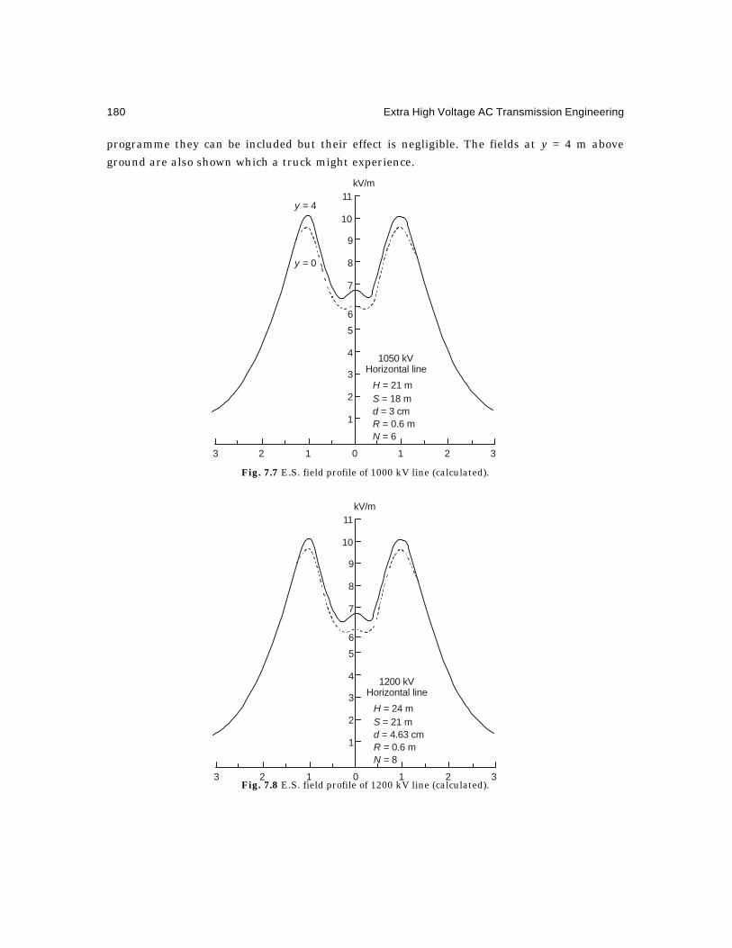
180 Extra High Voltage AC Transmission Engineering
programme they can be included but their effect is negligible. The fields at y = 4 m above
ground are also shown which a truck might experience.
Fig. 7.7 E.S. field profile of 1000 kV line (calculated).
Fig. 7.8 E.S. field profile of 1200 kV line (calculated).
3 2 1 0 1 2 3
1
2
3
4
5
6
7
8
9
10
11
1050 kVHorizontal line
H = 21 mS = 18 md = 3 cmR = 0.6 mN = 6
y = 0
y = 4
kV/m
3 2 1 0 1 2 3
1
2
3
4
5
6
7
8
9
10
11
1200 kVHorizontal line
H = 24 mS = 21 md = 4.63 cmR = 0.6 mN = 8
kV/m

Electrostatic and Magnetic Fields of EHV Lines 181
7.3.3 Electrostatic Field of Double-Circuit 3-phase A.C. LineOn a D/C line there are 6 conductors on a tower, neglecting ground wires above the lineconductors. [Some proposals for using shielding wires under the line conductors are made, butsuch problems will not be discussed in this book]. The e.s. field will depend on the phaseconfiguration of the two circuits and for illustrating the procedure, the arrangement shown inFig. 7.9 will be used. The positions occupied by the phases are numbered 1 to 6 and it is evidentthat (a) conductors 1 and 4 have the voltage ),(sin ϕ+wtVm (b) conductors 2 and 5 have voltages
)120(sin °−ϕ+wtVm and (c) conductors 3 and 6 have voltages ).120(sin °+ϕ+wtVm
Fig.7.9 Configuration of a double-circuit (D/C) line.
Consequently, the horizontal and vertical components of e.s. field will consist of 6 quantitiesas follows:
1hE = )()(sin)[(.2 1512141111
0
1 MMwtMMJVJe
qm ++ϕ++=
π
)]120(sin)()120(sin 1613 °+ϕ+++°−ϕ+ wtMMwt ...(7.23)
M
6hE = )()(sin)[(.2 6562646166
0
6 MMwtMMJVJe
qm ++ϕ++=
π)]120(sin)()120(sin 6663 °+ϕ+++°−ϕ+ wtMMwt ...(7.24)
where the Maxwell's Potential coefficient matrix [P] and its inverse [M] are now of order 6 × 6,and the Ji values are given from equation (7.16) by using i = 1, 2, ..., 6 in turn. Once again, the
total horizontal component of e.s. field at ),( yxA is of the form
Eht = Vm [Jh1 sin )120(sin)( 2 °−ϕ++ϕ+ wtJwt h )]120sin(.3 °+ϕ++ wtJh and in phasor form
htE = )120120( 321 °+ϕ∠+°−ϕ∠+ϕ∠ hhhm JJJV ...(7.25)
The quantities ,,, 321 hhh JJJ are obtained by adding equations (7.23) to (7.24) vertically
and collecting the coefficients of sin ).120(sinand)120(sin),( °+ϕ+°−ϕ+ϕ+ wtwtwt This is of
the same form as equation (7.19).
Similarly, the total vertical component of e.s. field can be obtained by using equation(7.17) for calculating K1 to K6. Then,
vtE = VKv .
1
2
3 4
5
6
A
B
C A'
B'
C'
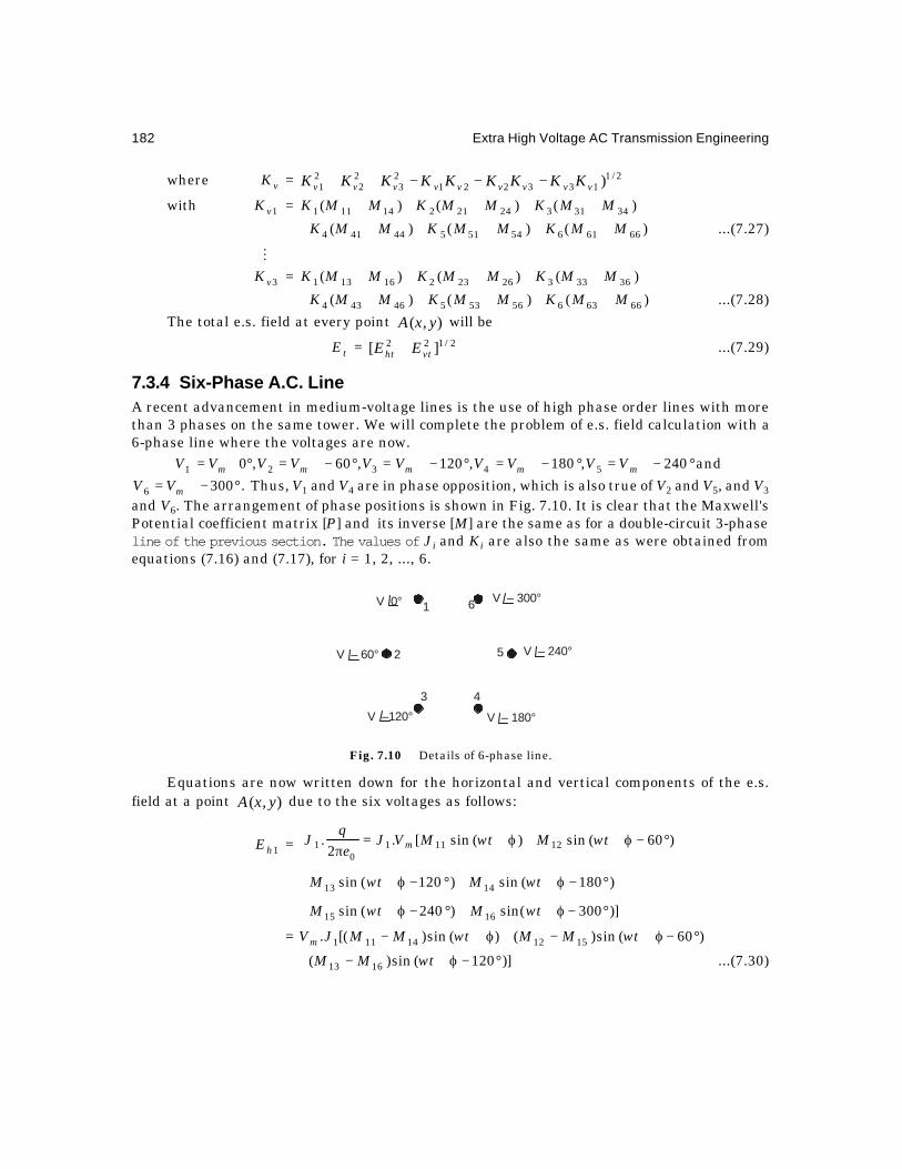
182 Extra High Voltage AC Transmission Engineering
where vK = 2/1133221
23
22
21 )vvvvvvvvv KKKKKKKKK −−−++
with 1vK = )()()( 343132421214111 MMKMMKMMK +++++
)()()( 666165451544414 MMKMMKMMK ++++++ ...(7.27)
M3vK = )()()( 363332623216131 MMKMMKMMK +++++
)()()( 666365653546434 MMKMMKMMK ++++++ ...(7.28)
The total e.s. field at every point ),( yxA will be
tE = 2/122 ][ vtht EE + ...(7.29)
7.3.4 Six-Phase A.C. LineA recent advancement in medium-voltage lines is the use of high phase order lines with morethan 3 phases on the same tower. We will complete the problem of e.s. field calculation with a6-phase line where the voltages are now.
and240,180,120,60,0 54321 °−∠=°−∠=°−∠=°−∠=°∠= mmmmm VVVVVVVVVV.3006 °−∠= mVV Thus, V1 and V4 are in phase opposition, which is also true of V2 and V5, and V3
and V6. The arrangement of phase positions is shown in Fig. 7.10. It is clear that the Maxwell'sPotential coefficient matrix [P] and its inverse [M] are the same as for a double-circuit 3-phaseline of the previous section. The values of Ji and Ki are also the same as were obtained fromequations (7.16) and (7.17), for i = 1, 2, ..., 6.
Fig. 7.10 Details of 6-phase line.
Equations are now written down for the horizontal and vertical components of the e.s.field at a point ),( yxA due to the six voltages as follows:
1hE = )60(sin)(sin[.2
. 121110
1 °−ϕ++ϕ+=π
wtMwtMVJe
qJ m
)180(sin)120(sin 1413 °−ϕ++°−ϕ++ wtMwtM
)]300sin()240(sin 1615 °−ϕ++°−ϕ++ wtMwtM
= )60(sin)()(sin)[(. 151214111 °−ϕ+−+ϕ+− wtMMwtMMJVm
)]120(sin)( 1613 °−ϕ+−+ wtMM ...(7.30)
1
2
3 4
5
6V 0°
V – 60°
V –120° V – 180°
V – 240°
V – 300°
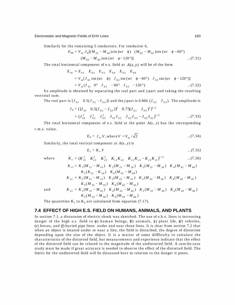
Electrostatic and Magnetic Fields of EHV Lines 183
Similarly for the remaining 5 conductors. For conductor 6,Eh6 = )60(sin)()(sin)[(. 656264616 °−ϕ+−+ϕ+− wtMMwtMMJVm
)]120(sin)( 6663 °−φ+−+ wtMM ...(7.31)
The total horizontal component of e.s. field at ),( yxA will be of the form
htE = 654321 hhhhhh EEEEEE +++++
= )]120(sin)60(sin)(sin[ 321 °−ϕ++°−ϕ++ϕ+ wtJwtJwtJV hhhm
= )120600( 321 °−∠+°−∠+°∠ hhhm JJJV ...(7.32)
Its amplitude is obtained by separating the real part and j-part and taking the resultingvectroial sum.
The real part is )](5.0[ 321 hhh JJJ −+ and the j-part is 0.866 ).( 32 hh JJ + The amplitude is
Jh =2/12
322
321 ])(75.0)(5.0[ hhhhh JJJJJ ++−+
= 2/1133221
23
22
21 )( hhhhhhhhh JJJJJJJJJ −++++ ...(7.33)
The total horizontal component of e.s. field at the point A(x, y) has the corresponding
r.m.s. value.
Eh = 2/where,. mh VVVJ = ...(7.34)
Similarly, the total vertical component at A(x, y) is
Ev = Kv.V ...(7.35)
where vK = 2/1133221
23
22
21 )( vvvvvvvvv KKKKKKKKK −++++ ...(7.36)
1vK = )()()()( 44414343132421214111 MMKMMKMMKMMK −+−+−+−
)()( 6461654515 MMKKKK −+−+
2vK = )()()()( 45424363232522215121 MMKMMKMMKMMK −+−+−+−
)()( 6562655525 MMKMMK −+−+and 3vK = )()()()( 46434363332623216131 MMKMMKMMKMMK −+−+−+−
)()( 6663656535 MMKMMK −+−+The quantities K1 to K6 are calculated from equation (7.17).
7.4 EFFECT OF HIGH E.S. FIELD ON HUMANS, ANIMALS, AND PLANTSIn section 7.1, a discussion of electric shock was sketched. The use of e.h.v. lines is increasingdanger of the high e.s. field to (a) human beings, (b) animals, (c) plant life, (d) vehicles,(e) fences, and (f) buried pipe lines under and near these lines. It is clear from section 7.2 thatwhen an object is located under or near a line, the field is disturbed, the degree of distortiondepending upon the size of the object. It is a matter of some diffficulty to calculate thecharacteristics of the distorted field, but measurements and experience indicate that the effectof the distorted field can be related to the magnitude of the undistorted field. A case-by-casestudy must be made if great accuracy is needed to observe the effect of the distorted field. Thelimits for the undistorted field will be discussed here in relation to the danger it poses.
184 Extra High Voltage AC Transmission Engineering
(a) Human BeingsThe effect of high e.s. field on human beings has been studied to a much greater extent
than on any other animals or objects because of its grave and shocking effects which hasresulted in loss of life. A farmer ploughing his field by a tractor and having an umbrella over hishead for shade will be charged by corona resulting from pointed spikes. The vehicle is alsocharged when it is stopped under a transmission line traversing his field. When he gets off thevehicle and touches a grounded object, he will discharge himself through his body which is apure resistance of about 2000 ohms. The discharge current when more than the let-go currentcan cause a shock and damage to brain.
It has been ascertained experimentally that the limit for the undisturbed field is 15 kV/m,r.m.s., for human beings to experience possible shock. An e.h.v. or u.h.v. line must be designedsuch that this limit is not exceeded. The minimum clearance of a line is the most importantgoverning factor. As an example, the B.P.A. of the U.S.A. have selected the maximum e.s. fieldgradient to be 9 kV/m at 1200 kV for their 1150 kV line and in order to do so used a minimumclearance at midspan of 23.2 m whereas they could have selected 17.2 m based on clearancerequired for switching-surge insulation recommended by the National Electrical Safety Council.
(b) AnimalsExperiments carried out in cages under e.h.v. lines have shown that pigeons and hens are
affected by high e.s. field at about 30 kV/m. They are unable to pick up grain because of chatteringof their beaks which will affect their growth. Other animals get a charge on their bodies andwhen they proceed to a water trough to drink water, a spark usually jumps from their nose tothe grounded pipe or trough.
(c) Plant LifePlants such as wheat, rice, sugarcane, etc., suffer the following types of damage. At a field
strength of 20 kV/m (r.m.s.), the sharp edges of the stalk give corona discharges so that damageoccurs to the upper portion of the grain-bearing parts. However, the entire plant does notsuffer dam age. At 30 kV/m , the by-products of corona, nam ely ozone and N 2O become intense.The resistance heating due to increased current prevents full growth of the plant and grain.Thus, 20 kV/m can be considered as the limit and again the safe value for a human beinggoverns line design.
(d) VehiclesVehicles parked under a line or driving through acquire electrostatic charge if their tyres
are made of insulating material. If parking lots are located under a line, the minimumrecommended safe clearance is 17 m for 345 kV and 20 m for 400 kV lines. Trucks and lorrieswill require an extra 3 m clearance. The danger lies in a human being attempting to open thedoor and getting a shock thereby.
(e) OthersFences, buried cables, and pipe lines are important pieces of equipment to require careful
layout. Metallic fences parallel to a line must be grounded preferably every 75 m. Pipelineslonger than 3 km and larger than 15 cm in diameter are recommended to be buried at least 30m laterally from the line centre to avoid dangerous eddy currents that could cause corrosion.Sail boats, rain gutters and insulated walls of nearby houses are also subjects of potentialdanger. The danger of ozone emanation and harm done to sensitive tissues of a human being athigh electric fields can also be included in the category of damage to human beings living neare.h.v. lines.

Electrostatic and Magnetic Fields of EHV Lines 185
7.5 METERS AND MEASUREMENT OF ELECTROSTATIC FIELDSThe principle on which a meter for measuring the e.s. field of an e.h.v. line is based is verysimple. It consists of two conducting plates insulated from each other which will experience apotential difference when placed in the field. This can be measured on a voltmeter or an ammeterthrough a current flow. There exist 3 configurations for the electrodes in meters used in practice:(1) Dipole, (2) Spherical Dipole, and (3) Parallel Plates. The dimensions and other details aregiven in the following tabular form. Also see Fig. 7.11.
Fig. 7.11 Measurement of E.S. field. (a) Dipole. (b) Spherical dipole. (c) Parallel plates.
Table 7.1 Meters for E.S. Field Measurement
(1) Electrode Shape Dipole Spherical Dipole Parallel Plates
(2) Major Dimensions Effective length, l Radius, r Distance, d,
Surface area, A
(3) Open-circuit Voltage E.l. – E.d
(as voltage source)
(4) Short-circuit Current Ewer 023π AEwe0
(as current source) – )3( 20reC π= )/( 0 dAeC =
The formula for the spherical dipole, which consists of two hemispheres insulated fromeach other, is very accurate and has been recommended as a standard. The two insulatedhemispheres are connected by a micro-ammeter whose scale is calibrated in terms of kV/m ofthe electric field. On the other hand, the parallel plate meter is very easy to fabricate. A smalldigital voltmeter can be used by attaching a copper-clad printed-circuit board with its insulatedside placed on top of the casing. The input to the meter is taken from the top copper-clad sideand the casing.
The procedure for measurement consists of attaching the meter to a long (2 m) insulatedrod and placing it in the field at the desired height. The insertion of the meter and rod as wellas the human-body should not distort the field.
The meters must be first calibrated in a high voltage laboratory. One procedure is tosuspend two horizontal plane parallel electrodes with constant separation. A suggested type is6 m × 6 m wire mesh electrodes separated by 1 m. These will be accurate to within 5%. Themeter is placed in the centre of this parallel-plate arrangement and a known voltage is graduallyapplied until about 100 kV/m is reached. The following application rules may be followed:
1. The instrument should be capable of measuring at least the vertical component ofelectric field. Up to a height of 3 or 4 m above ground, the horizontal component isvery small and the total 50 Hz field is nearly the same as its vertical component.
µA
r
(b)
SPHERICAL DIPOLE
A
d
(c)
PARALLEL PLATES
(a)
DIPOLE
l

186 Extra High Voltage AC Transmission Engineering
2. If the instrument is not held in hand, it should be mounted at about 2 m aboveground.
3. It should be battery powered in case a power supply for the electronic circuitry isnecessary.
4. The r.m.s. value is preferably measured by a full-wave rectifier circuit and suitablycalibrated.
5. Analogue indication may be preferable to digital representation as it disturbs thefield.
6. The instrument may have full-scale readings of 3, 10, 30, and 100 kV/m or othersuitable ranges for legible reading.
7. It should be designed for outdoor use and portable. A pole at least 2 m long must gowith the instrument if hand-held.
7.6 ELECTROSTATIC INDUCTION ON UNENERGIZED CIRCUIT OF A D/CLINE
We shall end this chapter with some discussion of electrostatic and electromagnetic inductionfrom energized lines into other circuits. This is a very specialized topic useful for line crew,telephone line interference etc. and cannot be discussed at very great length. EHV lines mustbe provided with wide enough right-of-way so that other low-voltage lines are located far enough,or when they cross the crossing must be at right angles.
Consider Fig. 7.12 in which a double-circuit line configuration is shown with 3 conductors
energized by a three-phase system of voltages )120sin(,sin 21 °−== wtVVwtVV mm and
V3 ).120(sin °+= wtVm The other circuit consisting of conductors 4, 5 and 6 is not energized.
We will calculate the voltage on these conductors due to electrostatic induction which a line-man may experience. Now,
4V = )/(ln2
)/(ln2
)/(ln2 3434
0
32424
0
21414
0
1 AIe
qAI
eq
AIe
qπ
+π
+π ...(7.37)
= 340
324
0
214
0
1
222P
eq
Pe
qP
eq
π+
π+
π
Fig. 7.12 D/C line: One line energized and the other unenergized to illustrate induction.
1
2
3 6
5
4
V wtm sin
V wt m sin ( – 120°)
V wt m sin ( + 120°)
V4
V5
V6
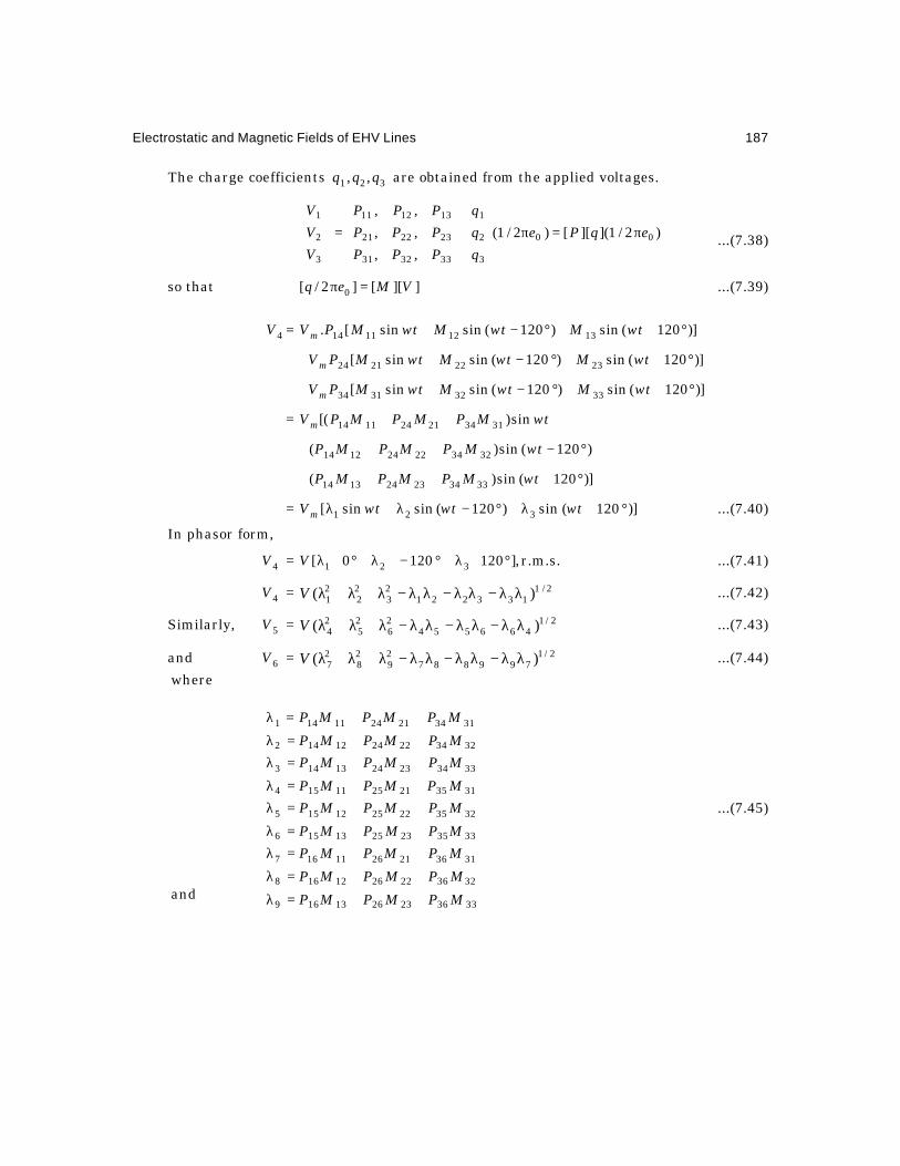
Electrostatic and Magnetic Fields of EHV Lines 187
The charge coefficients 321 ,, qqq are obtained from the applied voltages.
)2/1](][[)2/1(
,,
,,
,,
00
3
2
1
333231
232221
131211
3
2
1
eqPeqqq
PPPPPPPPP
VVV
π=π
=
...(7.38)
so that ]][[]2/[ 0 VMeq =π ...(7.39)
4V = )]120(sin)120(sinsin[. 13121114 °++°−+ wtMwtMwtMPVm
)]120(sin)120(sinsin[ 23222124 °++°−++ wtMwtMwtMPVm
)]120(sin)120(sinsin[ 33323134 °++°−++ wtMwtMwtMPVm
= wtMPMPMPVm sin)[( 313421241114 ++
)120(sin)( 323422241214 °−+++ wtMPMPMP
)]120(sin)( 333423241314 °++++ wtMPMPMP
= )]120(sin)120(sinsin[ 321 °+λ+°−λ+λ wtwtwtVm ...(7.40)
In phasor form,
4V = r.m.s.],1201200[ 321 °∠λ+°−∠λ+°∠λV ...(7.41)
4V = 2/1133221
23
22
21 )( λλ−λλ−λλ−λ+λ+λV ...(7.42)
Similarly, 5V = 2/1466554
26
25
24 )( λλ−λλ−λλ−λ+λ+λV ...(7.43)
and 6V = 2/1799887
29
28
27 )( λλ−λλ−λλ−λ+λ+λV ...(7.44)
++=λ
++=λ
++=λ++=λ
++=λ++=λ
++=λ++=λ
++=λ
3336232613169
3236222612168
3136212611167
3335232513156
3235222512155
3135212511154
3334232413143
3234222412142
3134212411141
MPMPMP
MPMPMP
MPMPMPMPMPMP
MPMPMPMPMPMP
MPMPMPMPMPMP
MPMPMP
...(7.45)
where
and

188 Extra High Voltage AC Transmission Engineering
Example 7.3. A 230-kV D/C line has the dimensions shown in Figure 7.13. The phaseconductor is a single Drake 1.108 inch (0.028 m) diameter. Calulate the voltages induced inconductors of circuit 2 when circuit 1 is energized assuming (a) no transposition, and (b) fulltransposition.
Fig. 7.13 D/C 230-kV line dimensions.
Solution. The Maxwell's Potential coefficients for the energized circuit are as follows:P11 = ln (36/0.014) = 7.852, P22 = ln (28/0.014) = 7.6,P33 = ln (20/0.014) = 7.264P12 = ln (32.02/4.19) = 2.0335, P13 = ln (28/8) =1.253,P23 = ln (24.03/4.19) = 1.747.
∴ [P]u = ;
264.7,747.1,253.1
747.1,6.7,0335.2
,253.1,0335.2,852.7
[M]ut =
−−−−−−
=−
14755.,0297.,0159.
0297.,1474.,0334.
0159.,0334.,1385.0
][ 1utP
P14 = ln (36.77/7.5) =1.59, P24 = ln (33.175/9.62) = 1.238,P34 = ln (29/10.97) = 0.972P15 = P24 = 1.238, P25 = ln (29.73/10) = 1.09,P35 = ln (25.55/9.62) = 0.9765P16 = P34 = 0.972, P26 = P35 = 0.9765,P36 = ln(21.36/7.5) = 1.0466.
These values give, from equations (7.42) to (7.45), with ,3/230=V
1λ = 0.1634, 2λ = 0.1005, 3λ = 0.0813, ∴ V4 = 9.76 kV.
4λ = 0.1196, 5λ = 0.09035, 6λ = 0.092, ∴ V5 = 3.9 kV.
7λ = 0.0854, 8λ = 0.0804, 9λ = 0.11, ∴ V6 = 3.65 kV.For the completely transposed line, the induced voltage is the average of these three
voltages which amounts to .kV77.5)65.39.376.9(31 =++
1
2
3 6
5
4
7.5
10
10
7.5
4
4

Electrostatic and Magnetic Fields of EHV Lines 189
7.7 INDUCED VOLTAGE IN INSULATED GROUND WIRESNormally, in all high voltage and e.h.v. lines which use overhead ground wires for lightningprotection, it is usual to tie them firmly to the tower top so that they are grounded directly andare at ground potential which is considered as zero. Consequently, only the phase conductorsexperience a voltage with respect to ground. However, in recent years, the shield wires strungabove the phase conductors are being insulated from the tower structure in order to utilizethem for the following purposes:
(a) To serve as conducting wires for carrier communication and protection. This is alsobeing taken over by fibre-optic links.
(b) To tap power at power frequency at a voltage lower than the power-frequencytransmission voltage in order to feed rural loads along the line route.
In order also to serve the primary purpose of shielding against lightning, the insulatorson which the "ground" wires are mounted should be provided with a spark gap which flashesover at the high lightning voltage. We will now discuss this problem of induced voltage oninsulated ground wires due to the power-frequency voltage carried by the phase conductors,assuming that the voltages of the shield wires are floating. The shield wires are made fromACSR instead of galvanized steel in order to reduce both the series resistance and inductance.
At first, the bundle charge on the three phase conductors (for a S/C line) are calculated atpower frequency in the usual manner from equation (7.4) or (7.38). Then, by using equations(7.37) to (7.42) and designating the insulated shield wires as 4,5,..., the voltage induced in themcan be calculated. For example, in a 400-kV line with two insulated shield wires, calculationyields an induced voltage of about 8.6% of the line-to-ground voltage of the phase condutorswhich amounts to roughly 21 kV, r.m.s., at 420 kV exccitation of the three phases, or about 20kV for 400 kV. This is shown in the following example.
Example 7.4. A 400-kV horizontal configuration S/C line of the UPSEB type has thedetails given in Example 4.16 in Chapter 4. The salient dimensions are as follows:
Phase conductors: Average height — 9.81 metres;Phase spacings — 11.3 metres;Conductor — 2 × 3.18 cm diameter at bundle
spacing of 45.72 cm.Ground wires: Height above ground — 20.875 metres. Neglect sag.
Horizontal spacing — 16 metres. Two numbers.Calculate the voltage induced in the insulated ground wires as a percentage of power-
frequency voltage of the phase conductors using the line-to-ground value.
Solution. The equivalent bundle radius is .m0815.0).( 2/1 == Brreq The Maxwell's
Potential Coefficients are as follows:
Self — P11 = P22 = P33 = ln (2 ×9.81/0.0815) = 5.44;Mutual—Outer to inner: P12 = P23 = 0.695;Outer to outer: P13 = 0.285.By inverting matrix [P] and evaluating the charge coefficients, there result for the phase
conductors, with V = phase-to-ground voltage,
01 2/ eq π = °∠×−°−∠×−°∠× −−− 120109.61201023010187 333 VVV
02 2/ eq π = °∠×−°−∠×+°∠×− −−− 1201023120107.18901023 333 VVV
03 2/ eq π = °∠×+°−∠×−°∠×− −−− 1201018712010230109.6 333 VVV

190 Extra High Voltage AC Transmission Engineering
Since the ground wires insulated from the tower are located symmetrically with respectto the phase conductors, the voltages induced in both will be equal. Designating any one ofthem as No. 4, the mutal potential coefficients between this wire and the three phase conductorsare calculated as follows:
Image distances: Aerial distances:
I14 = 2/122 ]3.3)81.9875.20[( ++ A14 = .5466.11]065.113.3[ 2/122 =+
= 30.864 metres;
I24 = ;m71.31]8685.30[ 2/122 =+ A24 = ;654.13]065.118[ 2/122 =+
I34 = ;m25.36]3.19685.30[ 2/122 =+ A34 = .m247.22]065.113.19[ 2/122 =+
∴ P14 = .4822.0:8426.0;9832.0)5466.11/864.30(ln 3424 === PP
Then, V4 = 340324021401 ).2/().2/().2/( PeqPeqPeq π+π+π= V]120065.0120126.001638.0[ °∠+°−∠+°∠
∴ V4/V = 126.01638.0065.0126.01638.0( 222 ×−++2/1)1638.0065.0065.0126.0 ×−×−
= %.634.808634.0)039476.0046931.0( 2/1 ==−
At V = 420 kV, line-to-line = ,kV3/420 line-to-ground,
V4 = 0.08634 × 242.49 = 20.94 kV to ground ≈ 21 kV, r.m.s.At 400 kV, V4 = 20 kV to groundThe insulator supporting the overhead shield wires must be rated for this voltage class.
7.8 MAGNETIC FIELD EFFECTSAn overhead line generates an electrostatic field in its vicinity because of the voltage at whichit is energized and the charge in its conductors trapped in its capacitance network. In addition,the line generates a magnetic field in its vicinity due to the load current flowing in the conductors.The intensity of the magnetic field is proportional to the currents so that it varies with the loadcondition. However, in e.h.v. lines, the load factor seldom if ever is lower than 75% so that theload current stays above 75% rated value most of the time. In calculating the magnetic field, wewill assume that the current flowing is the rated full-load current. The following Table givesthe values of rated current for e.h.v. lines based upon the details of Table 2 in Chapter II.
Nominal kV Reactance Length Load, MW 3ph Cond. Current, Amps.
400 0.327 400 km 612 883ohm/km 600 408 588at 50 Hz 800 306 441
500 0.3 400 1040 1200600 695 800800 520 600
750 0.272 600 1720 1327800 1290 9951000 1032 796
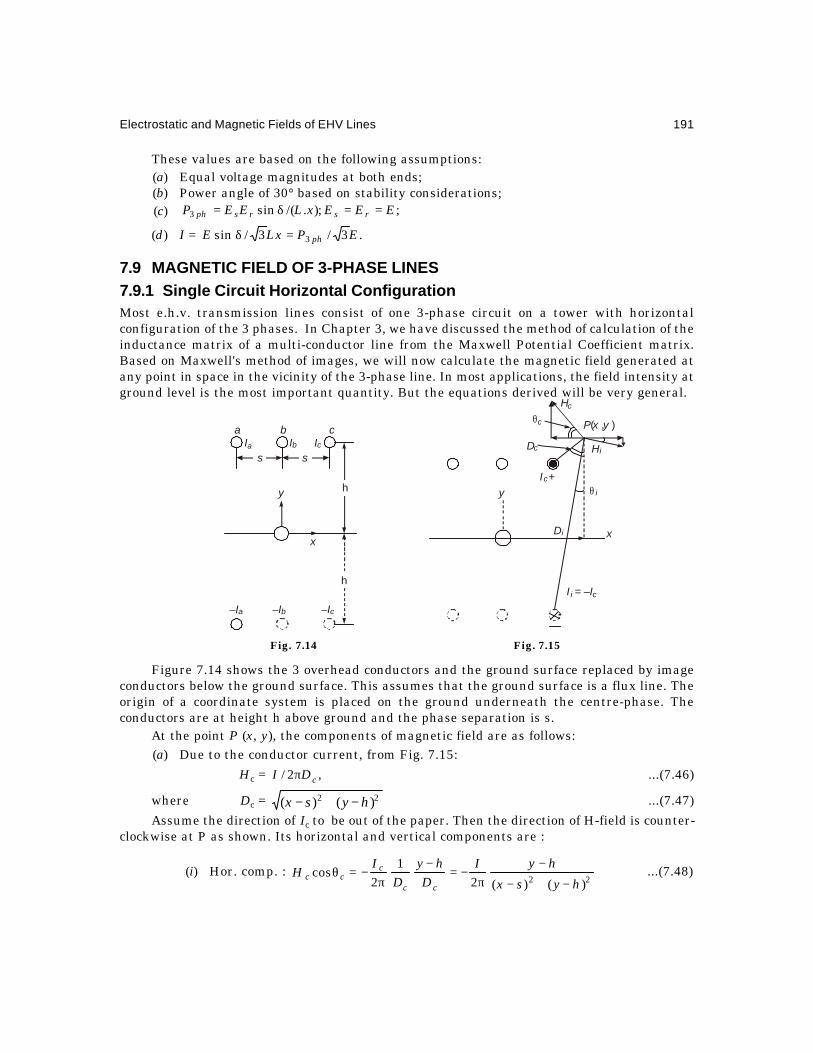
Electrostatic and Magnetic Fields of EHV Lines 191
These values are based on the following assumptions:(a) Equal voltage magnitudes at both ends;(b) Power angle of 30° based on stability considerations;(c) ;);./(sin3 EEExLEEP rsrsph ==δ=
(d) I = .3/3/sin 3 EPLxE ph=δ
7.9 MAGNETIC FIELD OF 3-PHASE LINES7.9.1 Single Circuit Horizontal ConfigurationMost e.h.v. transmission lines consist of one 3-phase circuit on a tower with horizontalconfiguration of the 3 phases. In Chapter 3, we have discussed the method of calculation of theinductance matrix of a multi-conductor line from the Maxwell Potential Coefficient matrix.Based on Maxwell's method of images, we will now calculate the magnetic field generated atany point in space in the vicinity of the 3-phase line. In most applications, the field intensity atground level is the most important quantity. But the equations derived will be very general.
Fig. 7.14 Fig. 7.15
Figure 7.14 shows the 3 overhead conductors and the ground surface replaced by imageconductors below the ground surface. This assumes that the ground surface is a flux line. Theorigin of a coordinate system is placed on the ground underneath the centre-phase. Theconductors are at height h above ground and the phase separation is s.
At the point P (x, y), the components of magnetic field are as follows:(a) Due to the conductor current, from Fig. 7.15:
Hc = ,2/ cDI π ...(7.46)
where Dc = 22 )()( hysx −+− ...(7.47)
Assume the direction of Ic to be out of the paper. Then the direction of H-field is counter-clockwise at P as shown. Its horizontal and vertical components are :
(i) Hor. comp. : 22 )()(2
12
coshysx
hyID
hyD
IH
cc
ccc
−+−
−π
−=−
π−=θ ...(7.48)
a b c
s
y
x
Ia
–Ia –Ib –Ic
Ib Ic
h
h
s
I i = –Ic
θc
θ i
Dc
Di
I +c
Hc
Hi
y
x
P x y( , )

192 Extra High Voltage AC Transmission Engineering
(ii) Vert. comp.: 22 )()(2
12
sinhysx
sxID
sxD
IH
cc
ccc
−+−
−π
=−
π=θ ...(7.49)
(b) Due to the image current:
Hi =22 )()(where,
12
hysxDD
Ii
i
c ++−=π ...(7.50)
This is directed in the clockwise sense as shown in Figure 7.15, since the current in theimage conductor is assumed to flow into the paper, opposite to the direction of current in theactual overhead conductor. The horizontal and vertical components of this magnetic field willbe:
(iii) Hor. comp.:22 )()(2
12
coshysx
hyID
hyD
IH c
ii
cii
++−
+π
=+
π=θ ...(7.51)
(iv) Vert. comp.:22 )()(2
12
sinhysx
sxID
sxD
IH c
ii
cii
++−
−π
−=−
π−=θ ...(7.52)
From the figure we observe that the horizontal and vertical components of Hc are directedin the opposite sense to those due to Hi. Therefore, the total horizontal and vertical componentsof the H-field at point P(x, y) due to the conductor current Ic and image current
Ii =– Ic will be readily seen to be:
Hh =
++−−−
++−+
π=θ+θ
2222 )()()()(2coscos
hysxhy
hysxhyIHH c
iicc Amp/metre. ...(7.53)
Hv =
++−−−
−+−−
π=θ+θ
2222 )()()()(2sinsin
hysxsx
hysxsxIHH c
iicc Amp/metre. ...(7.54)
The corresponding flux densities are:
Bh = ,,and, 00 TeslaHBH vvh µ=µ ...(7.55)
where 0µ = 7104 −×π Henry/metre.Following the above procedure, we can extend the equations to calculate the magnetic
field at P(x, y) due to the combined effect of all 3 conductor-currents. Let the three currents be:
Ia = Amps.120and,120,0 °+∠=°−∠=°∠ IIIII cb
Then: Hht =
−++−−
++++
π 2222 )()()()(2 hysxhy
hysxhyI a
−+−−
+++
π+
2222 )()(2 hyxhy
hyxhyIb
−+−−−
++−+
π+
2222 )()()()(2 hysxhy
hysxhyI c
, Amp/metre. ...(7.56)
Hvt =
++++−
−+++
π 2222 )()()()(2 hysxsx
hysxsxI a
Electrostatic and Magnetic Fields of EHV Lines 193
++−
−+π+
2222 )()(2 hyxx
hyxxIb
++−−−
−+−−
π+
2222 )()()()(2 hysxsx
hysxsxI c
, Amp/metre. ...(7.57)
In particular, on the ground surface where animals and human beings live, the magnetic-field components at a distance x from the line centre will be, with y = 0:
Hht = 222222 )(
22
22)(
22 hsx
hI
hx
hI
hsx
hI cba
+−π+
+π+
++π ...(7.58)
Hvt = .002
02)()(2 2222
=×π
+×π
+
+++−
+++
πcba II
hsxsx
hsxsxI
...(7.59)
Since we have assumed the ground surface to be a flux line, the vertical component of Hdue to any phase-current is zero, and the magnetic field at the ground surface is entirely in thehorizontal direction.
Magnitudes of Hht and Hvt. In equations (7.56) and (7.57), the three phase-currents Ia, Iband Ic are phasors with generally equal magnitudes I and having a phase difference of 120° withrespect to each other. They can be written as:
Ia = and);866.05.0(120);01(0 jIIIjII b −−=°−∠=+=°∠
Ic = ).866.05.0(120 jII +−=°+∠
It is convenient to abbreviate the six geometric factors from equations (7.56) and (7.57),thus:
Horizontal components:
Ka = 2222 )()()()( hysx
hy
hysx
hy
−++
−−
+++
+...(7.60)
Kb = 2222 )()( hyx
hy
hyx
hy
−+
−−
++
+...(7.61)
Kc = 2222 )()()()( hysx
hy
hysx
hy
−+−
−−
++−
+...(7.62)
Vertical components:
Ja = 2222 )()()()( hysx
sx
hysx
sx
+++
+−
−++
+...(7.63)
Jb = 2222 )()( hyx
x
hyx
x
++−
−+ ...(7.64)
Jc = 2222 )()()()( hysx
sx
hysx
sx
++−
−−
−+−
−...(7.65)
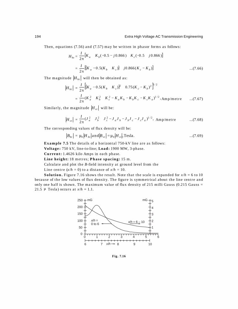
194 Extra High Voltage AC Transmission Engineering
Then, equations (7.56) and (7.57) may be written in phasor forms as follows:
Hht = [ ])866.05.0()866.05.0(2
jKjKKIcba +−+−−+
π
= [ ])(866.0)(5.02 bccba KKjKKKI −++−
π...(7.66)
The magnitude htH will then be obtained as:
htH = [ ] 2/122 )(75.0)(5.02 bccba KKKKKI −++−
π
= ,)(2
2/1222accbbacba KKKKKKKKKI −−−++
π Amp/metre ...(7.67)
Similarly, the magnitude vtH will be:
vtH = ,)(2
2/1222accbbacba JJJJJJJJJI −−−++
π Amp/metre ...(7.68)
The corresponding values of flux density will be:
htB = .Tesla,and 00 vtvtht HBH µ=µ ...(7.69)
Example 7.5 The details of a horizontal 750-kV line are as follows:Voltage: 750 kV, line-to-line; Load: 1900 MW, 3-phase.Current: 1.4626 kilo Amps in each phase.Line height: 18 metres; Phase spacing: 15 m.Calculate and plot the B-field intensity at ground level from theLine centre (x/h = 0) to a distance of x/h = 10.Solution. Figure 7.16 shows the result. Note that the scale is expanded for x/h = 6 to 10
because of the low values of flux density. The figure is symmetrical about the line centre andonly one half is shown. The maximum value of flux density of 215 milli Gauss (0.215 Gauss =21.5 µ Tesla) occurs at x/h = 1.1.
Fig. 7.16
6 7 8 9 10
0 1 2 3 4 5 6
x h/
x h/ = 0 to 6
x h/ = 6 – 10
1
2
3
4
5
0
50
100
150
200
250 mG mG
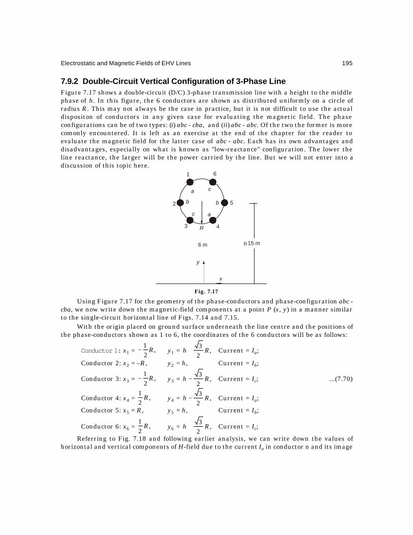
Electrostatic and Magnetic Fields of EHV Lines 195
7.9.2 Double-Circuit Vertical Configuration of 3-Phase LineFigure 7.17 shows a double-circuit (D/C) 3-phase transmission line with a height to the middlephase of h. In this figure, the 6 conductors are shown as distributed uniformly on a circle ofradius R. This may not always be the case in practice, but it is not difficult to use the actualdispositon of conductors in any given case for evaluating the magnetic field. The phaseconfigurations can be of two types: (i) abc - cba, and (ii) abc - abc. Of the two the former is morecomonly encountered. It is left as an exercise at the end of the chapter for the reader toevaluate the magnetic field for the latter case of abc - abc. Each has its own advantages anddisadvantages, especially on what is known as "low-reactance" configuration. The lower theline reactance, the larger will be the power carried by the line. But we will not enter into adiscussion of this topic here.
Fig. 7.17
Using Figure 7.17 for the geometry of the phase-conductors and phase-configuration abc -cba, we now write down the magnetic-field components at a point P (x, y) in a manner similarto the single-circuit horizontal line of Figs. 7.14 and 7.15.
With the origin placed on ground surface underneath the line centre and the positions ofthe phase-conductors shown as 1 to 6, the coordinates of the 6 conductors will be as follows:
Conductor 1: x1 = ,21
R− y1 = ,23
Rh + Current = Ia;
Conductor 2: x2 = –R, y2 = h, Current = Ib;
Conductor 3: x3 = ,21
R− y3 = ,23
Rh − Current = Ic; ...(7.70)
Conductor 4: x4 = ,21
R y4 = ,23
Rh − Current = Ia;
Conductor 5: x5 = R, y5 = h, Current = Ib;
Conductor 6: x6 = ,21
R y6 = ,23
Rh + Current = Ic;
Referring to Fig. 7.18 and following earlier analysis, we can write down the values ofhorizontal and vertical components of H-field due to the current In in conductor n and its image
1
2
6
3 4
5
a
b
c a
b
c
R
x
6 m
y
15 mh

196 Extra High Voltage AC Transmission Engineering
current –In. The values of n range from 1 to 6 for the indicated positions of the phase conductors.Conductor n has the coordinates ).,( nn yxC
Fig. 7.18
Magnetic Fields: See Fig. 7.18.
Due to the conductor current, Hc =c
n
DI 12π
...(7.71)
where 2cD = .)()( 22
nn yyxx −+− ...(7.72)
Its horizontal component is ccH θ− sin = 22 c
nn
DyyI −
π− ...(7.73)
The vertical component is + ccH θcos = 22 c
nn
DxxI −
π ...(7.74)
Due to the image current, Hi =i
n
DI 12π ...(7.75)
where 2iD = .)()( 22
nn yyxx ++− ...(7.76)
Its horizontal component is iiH θ+ cos = 22 i
nn
DyyI +
π ...(7.77)
The vertical component is iiH θ− sin = – 22 i
nn
DxxI −
π...(7.78)
The total horizontal component will be: hH =
−−
+π 222 c
n
i
nn
D
yy
D
yyI...(7.79)
Hc
Hiθi
Di
In
– In
yn
yn
ycnDc
θc
(xn,yn)
P x y( , )
x

Electrostatic and Magnetic Fields of EHV Lines 197
and total vertical component is vH =
−−
−π 222 i
n
c
nn
D
xx
D
xxI...(7.80)
Combining the effect of all 6 conductors, we can write down:
Hht =
−+−
−−
−++
+π 2
12
1
12
12
1
1
)()()()(2 yyxx
yy
xxyy
yyI a
−+−
−−
−++
++
24
24
42
42
4
4
)()()()( yyxx
yy
xxyy
yy
+ ( )
−+−
−−
++−
+π 2
22
2
22
22
2
2
)()()(2 yyxx
yy
yyxx
yyIb
−+−
−−
++−
++
25
25
52
52
5
5
)()()()( yyxx
yy
yyxx
yy
+
−+−
−−
++−
+π 2
32
3
32
32
3
3
)()()()(2 yyxx
yy
yyxx
yyIc
−+−
−−
++−
++
26
26
62
62
6
6
)()()()( yyxx
yy
yyxx
yy...(7.81)
= )(2
)(2
)(2 635241 KKIKKIKKI cba +
π++
π++
π ...(7.82)
= .222 c
cb
ba
a KIKIKIπ
+π
+π ...(7.83)
∴ htH =2/1222 )(
2 accbbacba KKKKKKKKKI −−−++π ...(7.84)
Similarly, the total vertical component of the H-field will be:
vtH =
++−
−−
−+−
−π 2
12
1
12
12
1
1
)()()()(2 yyxx
xx
yyxx
xxI a
++−
−−
−+−
−+
24
24
42
42
4
4
)()()()( yyxx
xx
yyxx
xx
+
++−
−−
−+−
−π 2
22
2
22
22
2
2
)()()()(2 yyxx
xx
yyxx
xxIb
++−
−−
−+−
−+
25
25
52
52
5
5
)()()()( yyxx
xx
yyxx
xx

198 Extra High Voltage AC Transmission Engineering
+
++−
−−
−+−
−π 2
32
3
32
32
3
3
)()()()(2 yyxx
xx
yyxx
xxIc
++−
−−
−+−
−+
26
26
62
62
6
6
)()()()( yyxx
xx
yyxx
xx...(7.85)
= )(2
)(2
)(2 635241 JJIJJIJJI cba +
π++
π++
π ...(7.86)
= cc
bb
aa JIJIJI
π+
π+
π 222...(7.87)
∴ vtH =2/1222 )(
2 accbbacba JJJJJJJJJI −−−++π ...(7.88)
Ground-level Field: Y = 0. Dc = Di.For this case, equations (7.81) and (7.85) are as follows:
Ka = 24
24
421
21
1
)(
2
)(
2
yxxy
yxxy
+−+
+− ...(7.89)
Kb = 25
25
522
22
2
)(
2
)(
2
yxxy
yxxy
+−+
+− ...(7.90)
Kc = 26
26
623
23
3
)(
2
)(
2
yxxy
yxxy
+−+
+− ...(7.91)
Ja = .beforeas0.0 =∴== vtcb HJJ
We notice that Ka, Kb, Kc as well as Ja, Jb, Jc in equations (7.82), (7.83), (7.86) and (7.87)have been written as the sum of two terms:
Ka = ;,, 635241 KKKKKKKK cb +=+=+ ...(7.92)
Ja = .,, 635241 JJJJJJJJ cb +=+=+ ...(7.93)One advantage in writing like this is that later on when we evaluate the magnetic field of
a 6-phase line, there will be 6 conductors. Their currents will be diplaced by 60° and it willprove easy to evaluate the resulting field. The values of x1 to x6 and y1 to y6 are given inequation (7.70).
Example 7.6. Figure 7.17 shows the details of a D/C 3-phase line. The line height to themiddle phases is 15 metres while the 6 conductors are distributed uniformly on a circle ofradius 6 m. The total 3-phase load is 240 MW at 230 kV, line-to-line, giving a current of 300Amps in each conductor.
Calculate and plot the magnitude of flux density near the line along the ground surfaceonly, as the distance from line centre is varied from x = 0 to x = 5 h = 75 metres.
Solution. At ground level, vtH = vtB = 0. Only the horizontal component survives.
The values of x1 to x6 and y1 to y6 are given in equations (7.70), where h = 15 m and R = 6 m.

Electrostatic and Magnetic Fields of EHV Lines 199
Figure 7.19 Shows the results of computation of the ground-level flux density. It has amaximum (r.m.s.) value of B = 40 mG at x/h = 0.4 and decreases or attenuates rapidly to nearlyzero at x/h = 4, or, x = 60 m from line centre.
Fig. 7.19
7.10 MAGNETIC FIELD OF A 6-PHASE LINEIn Fig. 7.17, let it be assumed that the currents in conductors 1 to 6 are as follows:
I1 = ),866.05.0(60,0 2 jIIII −=°−∠=°∠I3 = ,180),866.05.0(120 14 IIIIjII −=−=°−∠=−−=°−∠
I5 = ,)866.05.0(240 2IjII −=+−=°−∠ ...(7.94)
I6 = .)866.05.0(60300 3IjIII −=+=°∠=°−∠
Then, it is easy to observe that
htH = 66
55
44
33
22
11
222222KIKIKIKIKIKI
π+
π+
π+
π+
π+
π ...(7.95)
= [ 4321 )866.05.0()866.05.0(2
KjKjKKI −−−+−+π
])866.05.0()866.05.0( 65 jKjK +++−+ ...(7.96)
= [ ])(866.0)(5.02 6532653241 KKKKjKKKKKKI ++−−++−−+−
π...(7.97)
The magnitude of the horizontal component is
htH = [ 2653241 )(5.0
2KKKKKKI +−−+−
π
] ,)(75.02/12
6532 KKKK −−++ Amp/metre. ...(7.98)
The values of K1 to K6 can be obtained from equation (7.81).
Similarly, the magnitude of the vertical component of magnetic field is:
vtH = [ 2653241 )(5.0
2JJJJJJI +−−+−
π
] ,)(75.02/12
6532 JJJJ −−++ Amp/metre ...(7.99)
0 1 2 3 4
x h/
mG50
0

200 Extra High Voltage AC Transmission Engineering
where the values of J1 to J6 are obtained from equation (7.85).The corresponding flux densities are:
htB = ,and, 00 vtvtht HBH µ=µ Tesla. ...(7.100)
Example 7.7. Assume that a 138-kV 6-phase line with conductor-conductor voltage (andconductor-tower) voltage being equal to 138 kV. The conductors occupy the same positions asfor the 3-phase D/C line considered in Example 7.6 earlier. The load is also nearly equal and theconductor-current is 300 Amperes.
Calculate and plot the horizontal component of htB at ground level only.
Fig. 7.20
Solution. Figure 7.20 shows the result of calculating htB from equation (7.98) and (7.100)
at ground level, y = 0.
We observe that the maximum value of htB at ground level is 92 mG which is higher
than for an equivalent 3-phase D/C line shown in Fig. 7.19.
7.11 EFFECT OF POWER-FREQUENCY MAGNETIC FIELDS ON HUMANHEALTH
Magnetic fields are basically energy reservoirs with an energy density of e = ,/Joules,2/ 30
2 mB µwhere B is in Tesla and 7
0 104 −×π=µ Henry/metre. This energy is known to influence tissuesin the human body in everyday activities. Some of the effects are known to be beneficial such asbeing used medically for healing broken bones, but most are harmful and pose health hazardsamong which have been counted cancer of many types. These cancers are: leukemia or bloodcancer, lymphoma which weakens the immune system of the body to cancerous conditions,nervous disorders leading to brain damage such as altzheimer disease, breast cancer in bothfemale and male species, and several other dangerous conditions too numerous to enumerate
100
50
0
mG
0 1 2 3 4 5
x h/
Electrostatic and Magnetic Fields of EHV Lines 201
here. The magnetic radiation at low frequency emanating from Video Display Terminals suchas are used by secretaries in banks, offices and so on is suspected to cause not only skin rash,eye problems, tissue cancer but more importantly are known to give rise to spontaneous abortionsin pregnant women operators thereby forcing an end to pregnancy. The study of health hazardsassociated with power-frequency (50 and 60 Hz) magnetic fields has gained world-wide importancein medical, biological, physics and engineering fields and is the subject of intensive study,including the magnetic-field radiation from e.h.v. lines and distribution lines. We will onlydescribe and discuss a few basic facts and mechanisms that give rise to health hazards associatedwith magnetic fields.
It is also believed but not proved with certainty that the power-frequency magnetic fieldinduces a voltage in the tissue which in turn yields a current flow due to the electricalconductivity of the tissue (about 0.1 to 0.2 Siemen/metre). Some workers discount this theorybecause the cell walls are made from proteins which act as insulation barriers to the currentflow. Moreover, the energy fed by this mechanism is considered too low, below even the thermalor Johnson noise of the ions in the cell at the body temperature (37°C or 310°K). Therefore,other mechanisms are sought for to explain the influence of magnetic fields on cancer-producingconditions.
Some international organizations such as the World Health Organization (WHO),International Radiation Protection Association (IRPA) as also other national organizations ofdifferent countries have given guidelines for limiting the magnetic field in homes or in occupationssuch as line workers. In homes where children and adults live and the electrical wiring carriespower-frequency current, the resulting magnetic field experienced continuously has beensuspected to cause cancerous conditions in the occupants. This observation was published inmedical, biological and electrical literature for the first time in North America in 1979 by twoscientists in Denver City, Colorado State, U.S.A. Their names are Nancy Wertheimer andEdward Leeper, the former a psychiatrist with the Denver Department of Public Health andthe latter a physicist. Prior to that date in 1966, two Russian scientists had published theirreport on their findings that electricians working with electrical distribution lines — bothmales and females — experienced breast cancer. They suspected the magnetic field of thecurrent-carrying lines to be the primary cause and advised the government to limit the exposureof workers to the magnetic field. The resulting Russian guidelines are as follows.
Exposure Hours 1 2 3 4 5 6 7 8B-Field, Gauss 754 616 503 402 314 251 201 176(The reader should convert the Gauss values given above to Ampere/metre).
Since then many international and national organizations have suggested the same limits.This is known as an "occupational hazard".
For the general public the exposure is about 1 to 2 hourse per day in public places wherenearby distribution lines can give rise to exposure to magnetic fields. Also, in many countries,schools and shopping centres are located near high-voltage transmission lines and have beensuspected as causing cancerous conditions in the school-children and shop-workers. There aremany such instances of magnetic fields at power frequency being associated, along with othercauses, with cancer-producing circumstances.
According to the WHO and IRPA Guidelines, any cancerous or other internal health defectsinside the body can only be diagonozed by observing conditions on the surface of the body or by

202 Extra High Voltage AC Transmission Engineering
other diagnostic examinations. Based on experience gained all over the world, they have relatedthe measured current density on the surface of the body or organ with the following healthhazards:
Surface CurrentDensity, mA/m2 Health Effects<1 Absence of any established effects.1 –10 Minor biological effects reported.10 –100 Well-established effects:
(a) Visual defects (called Magneto-Phosphene effect);(b) Possible nervous-system defects.
100 – 1000 Changes in central nervous-system excitability(onset of brain damage) established; Stimulations thresholds;Possible health hazards.
> 1000 Extra systoles; Ventricular fibrillation (heart condition); Definitehealth hazards.
(Note: 2mA/m10( = ).1ììA/c
2
The surface current density measured on a cylindrical organ of radius r and electricalconductivity σ is related to the flux density at a frequency f as follows:
Jrms =2
rms Amp/m,rBfσπ ...(7.101)
where Jrms = rms value of current density,
Brms = rms value of flux density in Tesla,
f = frequency, Hz,
σ = electrical conductivity of the tissue, Siemens/metre,and r = radius of the cylinder, metre.This is derived as follows:
The flux density is .2where,sin2)( ftBtB rms π=ωω= It induces a voltage in the cylinder
of radius r equal to ,22/dB rms222 Bfrdtrv π=π= volts. On the surface, the resulting voltage
gradient is .22/ rmsfrBrve π=π= This gives an rms value of surface current density equal to
.Amp/m, 2rmsrmsrms rBfeJ σπ=σ=
Example 7.8. For a current density of 1 mA/m2 = 10–4 A/m2, with f = 50 Hz and σ = 0.2 S/m,calculate the values of Brms required to establish this current density on cylinders with r = 10inches (Torso), 5 inches (heart and head), 2.5 inches (arm), 1.0 inch, 0.5 inch and 0.25 inch(fingers).
Solution. From equation ,1
.)/(),101.7( rmsrms rfJB σπ= Tesla. (1 Tesla = 10,000 Gauss =
104 Gauss).
r, inches 10 5 2.5 1.0 0.5 0.25
Brms, Gauss 1.25 2.5 5 12.5 25 50

Electrostatic and Magnetic Fields of EHV Lines 203
The WHO and IRPA Guidelines recommend that for electrical workers a current densityof 5 mA/m2 should not be exceeded on the surface of the torso with a radius of 10 inches = 25cm. For the general public, the limit of current density on the torso is 1 mA/m2. At 1mA/m2,there is no onset of any visible health defect, while at 5 mA/m2 there is just a chance of somedefect but the workers are in general protected by a suitable uniform. Thus, the flux-densitylimits are about 5 Gauss for electrical workers and 1 Gauss for the general public.
There are considerations governing the limiting value of flux desnsity other than surfacecurrent density as proposed by the WHO and IRPA Guidelines. But these are highly specializedtopics and will not be discussed here.
Review Questions and Problems
1. What is the effect of high electrostatic fields on human beings under a line? Why doesa normal human being not experience a shock when walking underneath a line? Whydo birds survive even though they come into contact with e.h.v. lines ?
2. Describe the difference between primary shock current and secondary shock current.What is the meaning of 'let-go' current?
3. A 400-kV horizontal line has 2 conductors of 3.18 cm diameter in a bundle with B =0.4572 metre spacing. The line height and phase spacing are H = 15 m and S = 12 m.A D/C 230-kV line runs parallel to it with its centre 25 metres from the centre of the400 kV line. The heights of the conductors are 18, 14, and 10 metres with equalhorizontal spacings of 10 metres between conductors. Calculate the voltages inducedin the 3 conductors closest to the 400-kV line if the voltage is 420 kV, line-to-line.Assume both lines to be fully transposed.
4. A 1150 kV ∆ line has conductors at heights 26 m and 44 m with 24 m spacing betweenthe lowest conductors. Each phase is equipped with 8 × 46 mm diameter conductor ona circle of 1.2 metre diameter. At 1200 kV, calculate the e.s. field at ground level atdistances from the line centre d =0, 13, 26, 39, and 52 metres.
5. A double-circuit 400–kV line has conductors displaced 8 m from line centre. Theheights of conductors are 13, 23, 33 m above ground. A neighbouring D/C 220-kV linehas one circuit at 10 m horizontal separation from the nearest circuit of the 400-kVline. Its conductors are 10, 14, 18 m above ground. The conductors of the 400–kV lineare 2 × 3.18 cm dia with 45.72 cm spacing. Calculate: (a) The voltage induced in the 3conductors of one 400–kV circuit when the other circuit is energized at 420–kV. [28.4,9.85, 7.23 kV]. (b) The voltage induced in the conductors of the nearest 220–kV circuitwhen only one of the (closest) 400–kV circuits is energized at 420–kV, [12,77, 13.72,14.25 kV]. (c) Repeat (b) when both 400–kV circuits are energized at 420–kV. Assumephase voltages (a, b, c; c, b, a) for the two circuits for the top, middle, and bottomconductors. (The Maxwell's Potential coefficient Matrix for 400–kV line is now 6 ×6).
[21.5, 15.2, 14.74 kV].
(d) Compare cases (a), (b), and (c), and give your comments on the voltages experiencedby a lineman.

204 Extra High Voltage AC Transmission Engineering
6. Repeat worked example 7.5 for the 750-kV horizontal line when 50% seriescompensation is used and plot the lateral profile of the magnetic field on Fig. 7.16.
7. Repeat worked example 7.6 when the phase configuration is abc – abc. Compare theintensity of resulting magnetic field and superimpose on it the result of Example 7.6,Fig. 7.19. Which configuration results in more favourable circumstances as far aslower magnetic field near the line?
8. A 3–phase 230 kV D/C line has the dimensions shown, with all dimensions in metres.The phase configuration is abc – cba with currents as follows: °∠== 030061 IIAmps; .120300;120300 4352 °+∠==°−∠== IIII The origin of coordinate systemis at ground level under the line centre as shown. Evaluate the following:
Fig. 7.21
(a) Write down the coordinates of the 6 conductors : ).,(to),( 6611 yxyx
(b) Calculate and plot the intensity of the B-field along ground for x = 0 to x = 5 h,where h = 10 metres.
(c) Give the value of x at which the maximum B-field occurs.
9. A 6-phase transmission line has the same dimensions as the 3-phase 230 kV D/C lineof problem 8. Its conductors carry the same current of 300 Amps. Assume the currentsto be: I1 = 300∠0° Amps; I2 = 300∠ – 60°; I3 = 300∠ – 120°;
I4 = 300∠ – 180°; I5 = 300∠ – 240°; and I6 = 300∠ – 300°.
Calculate the intensity of the B-field along ground only for x/h = 0 to 5. Take theorigin of the coordinate system on ground under the line centre. Plot the values onthe same figure as in Problem 8 of the 230–kV D/C line.
10. Convert the B-values given in the table in Section 7.11 to H-values.
x
y
Pr-δGr.
h = 10 m
4 25
41
36
4
7.5
10
7.5

Electrostatic and Magnetic Fields of EHV Lines 205
11. (a) Using a limiting energy value of S = 5 x 10⁻³ Joule/kg per year of continuousexposure to a magnetic field, calculate the r.m.s. value of the B-field at 50 Hz that
should not be exceeded. Take tissue density of ./kg2000/gm23mcc ==δ
(b) Derive the formula µδ= ,/./2823.0rms fSB Tesla, where δ = tissue density inkg/m3, and f = frequency.
[Hint : Let ;sin2)( rms tBtB ω= Energy density ,2/2oBe µ= Joule/m3; If tissue
volume = V and weight = W, then the energy/kg = );/)(2/( 2 WVB oµ Average energy
per cycle ).2/(2rms δµ= oB Then calculate energy in 1 year which should be equated to
S Joule/kg.]
8.1 TRAVELLING WAVES AND STANDING WAVES AT POWERFREQUENCY
On an electrical transmission line, the voltages, currents, power and energy flow from thesource to a load located at a distance L, propagating as electro-magnetic waves with a finitevelocity. Hence, it takes a short time for the load to receive the power. This gives rise to theconcept of a wave travelling on the line which has distributed line parameters r, l, g, c per unitlength. The current flow is governed mainly by the load impedance, the line-charging currentat power frequency and the voltage. If the load impedance is not matched with the lineimpedance, which will be explained later on, some of the energy transmitted by the source isnot absorbed by the load and is reflected back to the source which is a wasteful procedure.However, since the load can vary from no load (infinite impedance) to rated value, the loadimpedance is not equal to the line impedance always; therefore, there always exist transmittedwaves from the source and reflected waves from the load end. At every point on the interveningline, these two waves are present and the resulting voltage or current is equal to the sum ofthe transmitted and reflected quantities. The polarity of voltage is the same for both but thedirections of current are opposite so that the ratio of voltage to current will be positive for thetransmitted wave and negative for the reflected wave. These can be explained mathematicallyand have great significance for determining the characteristics of load flow along a distributed-parameter line.
The same phenomenon can be visualized through standing waves. For example, consideran open-ended line on which the voltage must exist with maximum amplitude at the open endwhile it must equal the source voltage at the sending end which may have a different amplitudeand phase. For 50 Hz, at light velocity of 300 × 103 km/sec, the wavelength is 6000 km, so thata line of length L corresponds to an angle of (L × 360°/6000). With a load current present, anadditional voltage caused by the voltage drop in the characteristic impedance is also presentwhich will stand on the line. These concepts will be explained in detail by first considering aloss-less line (r = g = 0) and then for a general case of a line with losses present.
8Theory of Travelling Waves and Standing
Waves

Theory of Travelling Waves and Standing Waves 207
8.1.1 Differential Equations and Their SolutionsConsider a section of line ∆x in length situated at a distance x from the load end. The linelength is L and has distributed series inductance l and shunt capacitance c per unit length,which are calculated as discussed in Chapter 3. The inductance is ( xl ∆. ) and capacitance ( xc ∆. )of the differential length x∆ . The voltages on the two sides of l are )( xx VV ∆+ and Vx, whilethe currents on the two sides of c are (Ix + ∆Ix) and Ix. From Figure 8.1 the following equationscan be written down:
Fig. 8.1 Transmission line with distributed inductance and capacitance.
xxx VVV −∆+ )( = xx IxjwlV ).( ∆=∆ ...(8.1)
and xxx III −∆+ )( = xx VxjwcI ).( ∆=∆ ...(8.2)By making x∆ infinitesimal, the changes in voltage and current along the line are expressed
as differential equations thus:
dxdVx / = z. Ix and dIx/dx = y. Vx ...(8.3)
where z = jwl and y = jwc, the series impedance and shunt capacitive admittance at powerfrequency. Since all quantities are varying sinusoidally in time at frequency f = w/2π, the time-dependence is not written, but is implicit.
By differentiating (8.3) with respect to x and substituting the expressions for dVx /dx anddIx/dx, we obtain independent differential equations for Vx and Ix as follows:
22 /dxVd x = z. y. Vx = p2Vx ...(8.4)
and 22 /dxId x = xx IpIyz 2.. = ...(8.5)
where yzp .= = λπ== /2/ jvjwlcjw ...(8.6)
which is the propagation constant, v = velocity of propagation, and λ = wavelength.Equation (8.4) and (8.5) are wave equations with solutions
Vx =pxpx eBeA −+ ...(8.7)
and Ix = ).(/)/1( pxpxx eBeA
zp
dxdVz −−
=
= )( pxpx eBeAzy −− ...(8.8)
Ix
VRIR
∆x
∆x
∆x x
l.
c .
(a)
V Vx x + ∆
l ∆x.Ix Ix + ∆Ix
∆ Ix
∆x
Ix
Vx Vx
(b) (c)
c .

208 Extra High Voltage AC Transmission Engineering
The two constants A and B are not functions of x but could be possible functions of t sinceall voltages and currents are varying sinusoidally in time. Two boundary conditions are nownecessary to determine A and B. We will assume that at x = 0, the voltage and current are VR
and IR. Then, A + B = VR and A – B = Z0IR, where Z0 = clyz // = = the characteristicimpedance of the line.
Then, Vx =λπ−λπ −++ /2
0/2
0 )(21
)(21 xj
RRxj
RR eIZVeIZV ...(8.9)
and Ix =λπ−λπ −−+ /2
0/2
0 )/(21
)/(21 xj
RRxj
RR eIZVeIZV ...(8.10)
We can also write them as
Vx = )/2sin()/2cos(. 0 λπ+λπ xIjZxV RR ...(8.11)
and Ix = )/2sin()./()/2cos(. 0 λπ+λπ xZVjxI RR ...(8.12)
Now, both VR and IR are phasors at power frequency and can be written as VR = )(. φ+jwtR eV ,
and )][(exp. LRR jwtII φ−φ+= where φL = internal angle of the load impedance ZL∠φL.
We can interpret the above equations (8.11) and (8.12) in terms of standing waves asfollows:
(1) The voltage Vx at any point x on the line from the load end consists of two parts: VR
cos )/2( λπx and jZ0 IR sin )/2( λπx . The term )/2cos( λπxVR has the value VR at x = 0(the load end), and stands on the line as a cosine wave of decreasing amplitude as xincreases towards the sending or source end. At x = L, it has the value )/2cos(. λπLVR .
This is also equal to the no-load voltage when IR = 0. Figure 8.2(a) shows thesevoltages. The second term in equation (8.11) is a voltage contributed by the load
current which is zero at x = 0 and Z0 IR sin )/2( λπL at the source end x = L, and addsvectorially at right angles to IR as shown in Figure 8.2 (c).
Fig. 8.2. Standing waves of (a) voltage, and (b) current at power frequency.
V LR cos 2 /λπ I LR cos 2 /λπ
jZ L0 sin 2 /λIR π
VR π cos 2 /L λ
VRIR
VR IR
L
L L
L θL
Z0I LR sin 2 /π λ VR Ζ 0
sin 2 /π λLVR Ζ 0
sin 2 /π λLj
2 πλLIR cos IR
VR
( )a ( )b ( )c

Theory of Travelling Waves and Standing Waves 209
(2) The current in equation (8.12) also consists of two parts. IR cos )/2( λπx and
)/2sin()/( 0 λπxZVj R . At no load, IR = 0 and the current supplied by the source is)/( 0ZVj R sin )/2( λπL which is a pure charging current leading VR by 90°. These are
shown in Fig. 8.2(b) and the vector diagram of 8.2(c).A second interpretation of equations (8.9) and (8.10) which are equivalent to (8.11) and (8.12)
is through the travelling wave concept. The first term in (8.9) is )/(0 )(
21 vxtjw
RR eIZV ++ after
introducing the time variation. At x = 0, the voltage is (VR + Z0 IR)/2 which increases as x does,
i.e., as we move towards the source. The phase of the wave is )/( vxtjwe + . For a constant value of(t + x/v), the velocity is dx/dt = – v. This is a wave that travels from the source to the load and
therefore is called the forward travelling wave. The second term is 21
)/(0 )( vxtjw
RR eIZV −− with
the phase velocity dx/dt = + v, which is a forward wave from the load to the source or a backwardwave from the source to the load.
The current also consists of forward and backward travelling components. However, forthe backward waves, the ratio of voltage component and current component is (–Z0) is seen bythe equations (8.9) and (8.10) in which the backward current has a negative sign before it.
8.2 DIFFERENTIAL EQUATIONS AND SOLUTIONS FOR GENERAL CASEIn Section 8.1, the behaviour of electrical quantities at power frequencies on a distributed-parameter line was described through travelling-wave and standing-wave concepts. The timevariation of all voltages and currents was sinusoidal at a fixed frequency. In the remainingportions of this chapter, the properties and behaviour of transmission lines under any type ofexcitation will be discussed. These can be applied specifically for lightning impulses and switchingsurges. Also, different types of lines will be analyzed which are all categorized by the fourfundamental distributed parameters, namely, series resistance, series inductance, shuntcapacitance and shunt conductance. Depending upon the nature of the transmitting medium(line and ground) and the nature of the engineering results required, some of these fourparameters can be used in different combinations with due regard to their importance for theproblem at hand. For example, for an overhead line, omission of shunt conductance g ispermissible when corona losses are neglected. We shall develop the general differential equationsfor voltage and current by first considering all four quantities (r, l, g, c) through the method ofLaplace Transforms, studying the solution and interpreting them for different cases when oneor the other parameter out of the four loses its significance. As with all differential equationsand their solutions, boundary conditions in space and initial or final conditions in time play avital role.
8.2.1 General Method of Laplace TransformsAccording to the method of Laplace Transform, the general series impedance operator per unitlength of line is z(s) = r + ls, and the shunt admittance operator per unit length is y(s) = g + cs,where s = the Laplace-Transform operator.
Consider a line of length L energized by a source whose time function is e(t) and LaplaceTransform E(s), as shown in Fig. 8.3. Let the line be terminated in a general impedance Zt(s).

210 Extra High Voltage AC Transmission Engineering
We will neglect any lumped series impedance of the source for the present but include it lateron. Also, x = 0 at the terminal end as in Section 8.1.2. Let the Laplace Transforms of voltageand current at any point x be V(x, s) and I(x, s).
Fig. 8.3 Distributed-parameter transmission line with source E(s) and terminating impedance Zt(s).
Then, the following two basic differential equations will hold as for the steady-stateexcitation discussed earlier:
xsxV ∂∂ /),( = ),().(./),(and),().( sxVsyxsxIsxIsz =∂∂ ...(8.13)
For simplicity in writing, we may omit s in all terms but only remember that we arediscussing the properties of the Laplace-Transforms of all quantities. The solutions for voltageand current in equation (8.13) will be
V(x) = pxpx eBeA −+ .. ...(8.14)
and I(x) = )).(/( pxpx BeAezp −− ...(8.15)
where again, p = the propagation constant = yz. ...(8.16)
Also, 0/)/( Yzyzp == and 0/)/( Zyzpz == , the characteristic or surge impedance.
For this problem, the boundary conditions are:(1) At x = L, V(L) = source voltage = E(s); and(2) At x = 0, V(0) = Zt. I(0). Using them in (8.14) and (8.15) yields
A = ])()/[()()( 000pL
tpL
tt eZZeZZsEZZ −−+++ ...(8.17)
and B = )/()( 00 ZZAZZ tt +− ...(8.18)
∴ V(x) = )(sinh)/(coshsinh)/(cosh
0
0 sEpLZZpLpxZZpx
t
t
++
...(8.19)
and I(x) = )(sinh)/(coshcosh)/(sinh
.1
0
0 sEpLZZpLpxZZpx
zy
xV
z t
t
++
=∂∂
...(8.20)
These are the general equations for voltage V and current I at any point x on the line inoperational forms which can be applied to particular cases as discussed below.
Line TerminationsFor three important cases of termination of an open-circuit, a short circuit and Zt = Z0,
the special expressions of equations (8.19) and (8.20) can be written.Case 1. Open Circuit. Zt = ∞
=
=
pLsEpxzysxI
pLsEpxsxV
oc
oc
cosh/)(.sinh./),(
cosh/)(.cosh),(...(8.21)
Vx V0
L0Ixe t( ) ZtE s( )
Lx
S r, l, g, c

Theory of Travelling Waves and Standing Waves 211
Case 2. Short-Circuit . Zt = 0
=
=
pLsEpxzysxI
pLsEpxsxV
sc
sc
sinh/)(.cosh/),(
sinh/)(.sinh),(...(8.22)
Case 3. Matched Line. Zt = Z0
++=
++=
)sinh/(cosh)().sinh(cosh/),(
)sinh/(cosh)().sinh(cosh),(
pLpLsEpxpxzysxI
pLpLsEpxpxsxV
m
m...(8.23)
The ratio of voltage to current at every point on the line is
Z0 = yz / .
0/[ Yzy = = .]/1)/()( 0Zlsrcsg =++Source of ExcitationThe time-domain solution of all these operational expressions are obtained through their
Inverse Laplace Transforms. This is possible only if the nature of source of excitation and itsLaplace Transform are known. Three types of excitation are important:
(1) Step Function. e(t) =V ; E(s) = V/s, where V = magnitude of step(2) Double-Exponential Function. Standard waveshapes of lightning impulse and switching
impulse used for testing line and equipment have a shape which is the difference between twoexponentials. Thus e(t) = E0 )( tt ee β−α− − where E0, α and β depend on the timings of importantquantities of the wave and the peak or crest value. The Laplace Transform is
E(s) = ))(/()(0 β+α+α−β ssE ...(8.24)
(3) Sinusoidal Excitation. When a source at power frequency suddenly energises atransmission line through a circuit breaker, considering only a single-phase at present, at anypoint on the voltage wave, the time function is e(t) = Vm sin )( φ+wt , where fw π= 2 , f = thepower frequency, and φ = angle from a zero of the wave at which the circuit breaker closes onthe positively-growing portion of the sine wave. Its Laplace Transform is
E(s) = )/()sin.cos.( 22 wsswVm +φ+φ ...(8.25)
Propagation Factor. For the general case, the propagation factor is
p = ))((. csglsryz ++= ...(8.16)
In the sections to follow, we will consider particular cases for the value of p, by omittingone or the other of the four quantities, or considering all four of them.
Voltage at Open-End. Before taking up a detailed discussion of the theory and propertiesof the voltage and current, we might remark here that for the voltage at the open end, equation(8.21) gives
V(0, s) = )/()(.2cosh/)( pLpL eesEpLsE −+== ...))((2 53 −+− −−− pLpLpL eeesE ...(8.26)
Under a proper choice of p this turns out to be a train of travelling waves reflecting fromthe open end and the source, as will be discussed later. Equation (8.26) also gives standingwaves consisting of an infinite number of terms of fundamental frequency and all its harmonics.
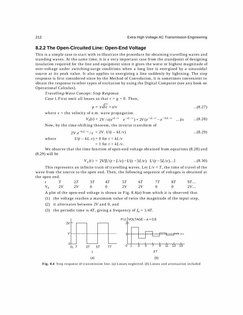
212 Extra High Voltage AC Transmission Engineering
8.2.2 The Open-Circuited Line: Open-End VoltageThis is a simple case to start with to illustrate the procedure for obtaining travelling waves andstanding waves. At the same time, it is a very important case from the standpoint of designinginsulation required for the line and equipment since it gives the worst or highest magnitude ofover-voltage under switching-surge conditions when a long line is energized by a sinusoidalsource at its peak value. It also applies to energizing a line suddenly by lightning. The stepresponse is first considered since by the Method of Convolution, it is sometimes convenient toobtain the response to other types of excitation by using the Digital Computer (see any book onOperational Calculus).
Travelling-Wave Concept: Step ResponseCase 1.First omit all losses so that r = g = 0. Then,
p = vslcs /= ...(8.27)
where v = the velocity of e.m. wave propagation.
∴ V0(s) = seeVeesV vsLvsLvsLvsL /...)(2)(/2 /3/// +−=+ −−− ...(8.28)
Now, by the time-shifting theorem, the inverse transform of
seV vksL /.2 /− = 2V. U(t – kL/v) ...(8.29)
where U(t – kL.v) = 0 for t < kL/v= 1 for t > kL/v.
We observe that the time function of open-end voltage obtained from equations (8.28) and(8.29) will be
)(0 tV = )/5()/3()/([2 vLtUvLtUvLtUV −+−−− ...] ...(8.30)
This represents an infinite train of travelling waves. Let L/v = T, the time of travel of thewave from the source to the open end. Then, the following sequence of voltages is obtained atthe open end.
t T 2T 3T 4T 5T 6T 7T 8T 9T...V0 2V 2V 0 0 2V 2V 0 0 2V...
A plot of the open-end voltage is shown in Fig. 8.4(a) from which it is observed that(1) the voltage reaches a maximum value of twice the magnitude of the input step,
(2) it alternates between 2V and 0, and
(3) the periodic time is 4T, giving a frequency of f0 = 1/4T.
Fig. 8.4 Step response of transmission line. (a) Losses neglected. (b) Losses and attenuation included
2V
V
001 T 3T 5T 7T
t
( )a
2
1
0 1 3 5 7 9 11 13 15
t T/
( )b
P.U. VOLTAGE – = 0.8a
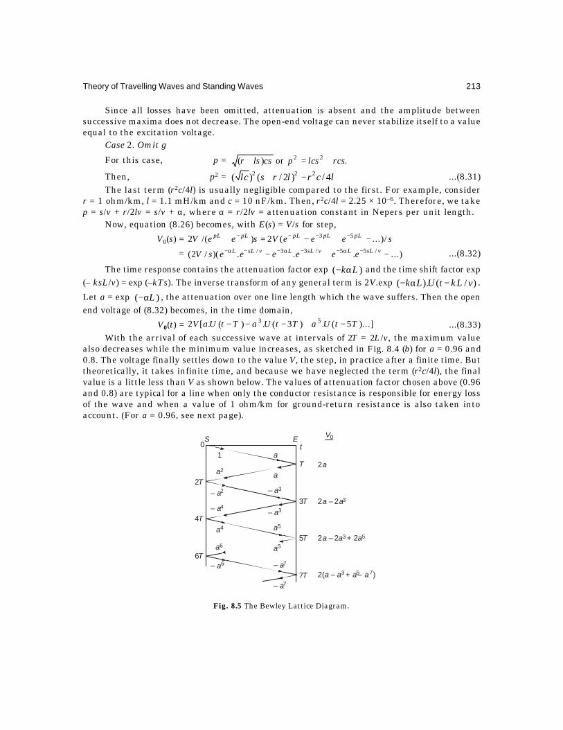
Theory of Travelling Waves and Standing Waves 213
Since all losses have been omitted, attenuation is absent and the amplitude betweensuccessive maxima does not decrease. The open-end voltage can never stabilize itself to a valueequal to the excitation voltage.
Case 2. Omit g
For this case, p = .or)( 22 rcslcspcslsr +=+
Then, p2 = lcrlrslc 4/)2/()( 222 −+ ...(8.31)The last term (r2c/4l) is usually negligible compared to the first. For example, consider
r = 1 ohm/km, l = 1.1 mH/km and c = 10 nF/km. Then, r2c/4l = 2.25 × 10⁻⁶. Therefore, we takep = s/v + r/2lv = s/v + α, where α = r/2lv = attenuation constant in Nepers per unit length.
Now, equation (8.26) becomes, with E(s) = V/s for step,
V0(s) = seeeVseeV pLpLpLpLpL /...)(2)/(2 53 −+−=+ −−−−
= ...)...)(/2( /55/33/ −+− −α−−α−−α− vsLLvsLLvsLL eeeeeesV ...(8.32)
The time response contains the attenuation factor exp )( Lkα− and the time shift factor exp(– ksL/v) = exp (–kTs). The inverse transform of any general term is 2V.exp )/().( vkLtULk −α− .
Let a = exp )( Lα− , the attenuation over one line length which the wave suffers. Then the openend voltage of (8.32) becomes, in the time domain,
V0(t) = )...]5(.)3(.)(.[2 53 TtUaTtUaTtUaV −+−−− ...(8.33)With the arrival of each successive wave at intervals of 2T = 2L/v, the maximum value
also decreases while the minimum value increases, as sketched in Fig. 8.4 (b) for a = 0.96 and0.8. The voltage finally settles down to the value V, the step, in practice after a finite time. Buttheoretically, it takes infinite time, and because we have neglected the term (r2c/4l), the finalvalue is a little less than V as shown below. The values of attenuation factor chosen above (0.96and 0.8) are typical for a line when only the conductor resistance is responsible for energy lossof the wave and when a value of 1 ohm/km for ground-return resistance is also taken intoaccount. (For a = 0.96, see next page).
Fig. 8.5 The Bewley Lattice Diagram.
S E0
2T
T
tV0
4T
3T
6T
5T
7T
1 a
aa2
– a2 – a3
– a3– a4
a4 a5
a5a6
– a6 – a7
– a7
2a
2a – a2 3
2 2a – a + a3 52
2(a – a + a– a3 5 7)

214 Extra High Voltage AC Transmission Engineering
The following tabular form gives a convenient way of keeping track of the open-end voltageand Fig. 8.5 shows a graphical sketch which is due to Bewley. It is known as the Bewley LatticeDiagram. Note the systematic method employed in finding the voltage after any number ofreflections.
Time t/T V0 (t) a = 0.96 a = 08
1 V1 = 2V.a 1.92 V 1.6 V2 V2 = 2V.a3 V3 = 2V(a – a3) = V1 – a2V1 0.15 V 0.576 V4 V4 = V3
5 V5 = 2V(a – a3 + a5) = V1 – a2V3 1.78 V 1.23 V6 V6 = V5
7 V7 = 2V(a – a3 + a5 – a7) = V1 – a2V5 0.28 V 0.81 V8 V8 = V7
9 V9 = 2V(a – a3 + a5 – a7 + a9) = V1 – a2V7 1.66 V 1.08 V10 V10 = V9
N VN = V1 – a2VN – 2
N + 1 VN +1 = VN
According to this procedure, the final value is
∞V = )1/(2...)1(2 2642 aVaaaaVa +=+−+− ...(8.34)
Example 8.1. For a = 0.96 and 0.8, find the final value of open-end voltage and the %error caused by omitting the term (r2c/4l) in equation (8.31)
Solution. (a) a = 0.96, ∞V = 0.9992 V, error = 0.08%.
(b) a = 0.8, ∞V = 0.9756 V, error = 2.44%.
8.2.3 The Bewley Lattice DiagramBefore we consider another form for p, let us discuss the Lattice Diagram for keeping accountof the infinite number of reflections on a line when suddenly energized by a source. A horizontalline is drawn to represent the line and two vertical lines at the ends on which equal intervals oftime T are marked as shown. The diagram begins at the top left corner at the source andproceeds along the line OT. The attenuation a is also shown for one travel. At the open end, thewave reflects completely as a. To the right is marked 2a which is the voltage at the open endafter one travel time. Arrows show the progress of the wave. At T, the wave reflects andreaches the source at time 2T with an amplitude a2, and since the source voltage has to remainconstant at + 1, the wave arriving at the source is reflected negatively and shown as – a2. Whenthis reaches the open end at time 3T, it has the value (– a3). Again, at the end, this wavedoubles and a reflection (– a3) travels back to the source. The total voltage at the open end isnow (a + a – a3 – a3) = 2(a – a3) which is the sum of all voltages marked on the inclined lines upto time 3T. Proceeding in this manner, we observe that in order to keep the source voltage at+ 1, continued reflections have to take place with negative signs at the source and positivesigns at the open end.
Theory of Travelling Waves and Standing Waves 215
8.2.4 r/l = g/c = ββIf the above condition is satisfied, then
p = vscgslrslccsglsr /)()]/)(/[())(( 2/1 β+=++=++
= s/v + r/lv. ...(8.35)
The step response is the same as before in Section 8.2.2 and Fig. 8.4(b), but the attenuationfactor is now b = exp (–βL/v) = exp (– 2αL/v) = a2. The voltage attenuates more rapidly thanwhen g = 0.
Example 8.2. For a = 0.96 and 0.8, find the resulting attenuation factor when r/l = g/c,assuming line length L to be equal in both cases. Also calculate the maximum values of thesurge in the two cases in p.u.
Solution. (1) a = Le α− = 0.96 ∴ b = a2 = 0.9216
Maximum value of surge is the first peak = 1.8432 p.u.(2) a = e–αL = 0.8. ∴ b = a2 = 0.64.
∴ First peak = 1.28 p.u.The relation r/l = g/c is also known as the distortionless condition in which any waveshape
of voltage applied at one end will travel without distortion of waveshape but will be attenuated.The relation is very useful in telephone and telegraph work where artificial loading coils areused to increase the value of inductance in cable transmission for which g and c are high whilel is low.
The case of including all four parameters (r, l, g, c) in the propagation constant p leads tocomplicated expressions for the Inverse Laplace Transform involving Bessel Functions but, aswill be shown in the next section, will yield easier solutions when the standing wave concept isresorted to.
8.3 STANDING WAVES AND NATURAL FREQUENCIESIn this method, the inverse Laplace Transform is evaluated by the Method of Residues andinstead of an infinite number of reflections caused by both ends, we obtain the solution as thesum of an infinite number of frequencies which consist of a fundamental frequency and itsharmonics. The infinite series of terms can be truncated after any suitable number of harmonicsto yield engineering results. We will first show that the method yields the same result as thetravelling-wave concept for a simple case, and then proceed with the Standing-wave Method for
more complicated cases for p = .))(( csglsr ++
8.3.1 Case 1–Losses Neglected r = g = 0The Laplace Transform of the open-end voltage, equation (8.26), can be written as (with r = g =0), for a step input,
V0 = V/s. cosh pL = V/s. cosh (s Llc ) ...(8.36)
The locations of the poles of the expression where the denominator becomes zero are firstdetermined. Then the residues at these poles are evaluated as described below, and the timeresponse of the open-end voltage is the sum of residues at all the poles.

216 Extra High Voltage AC Transmission Engineering
Location of Poles. The denominator is zero whenever s = 0 and 0cosh =Llcs . Now,cosh jθ = cos θ which is zero whenever 0,2/)12( =π+±=θ nn , 1, 2,... Thus, there are an infinite
number of poles where )cosh( Llcs becomes zero. They are located at
Lslc = 2/)12( π+± nj .
∴ s = 2/)12(and2/)12( π+±=±=π+± njpLjwcLlnj n ...(8.37)
where wn = TnLvncLln 2/)12(2/)12(2/)12( π+=π+=π+ ...(8.38)
upon using the property that lcv /1= and T = L/v. We also observe that (lL) and (cL) arethe total inductance and capacitance of the line of length L, and 024/22/ fTT π=π=π , with f0 =fundamental frequency. This was the same as was obtained in the travelling-wave concept.
ResiduesIn order to calculate the residue at a simple pole, we remove the pole from the denominator,
multiply by est and evaluate the value of the resulting expression at the value of s given at thepole.
(1) At s = 0:
Residue = VLslc
eV
s
st
==0)cosh(
., the input step.
(2) At the infinite number of poles, the procedure is to take the derivative of (cosh pL)with respect to s and evaluate the value of the resulting expression at each value of s at whichcosh pL = 0. Thus, the residues at the poles of (cosh pL) are found by the operation
)( +nV =
2/)12(
)(coshπ+=
=njpL
jws
st
npL
dsd
esV
...(8.39)
Now, dsd
cosh pLLlcLslcLlcLslc sinh.).sinh(.. == . But at ,2/)12( π+= njpLnjnjpL )1(2/)12sin(sinh −=π+= .
∴ V(n+) = π+−−=−
)12/()(exp2..)1(..)1(
)exp(. ntjwV
Llcj
tjwjwV
nn
nn
n...(8.40)
upon using equation (8.38).Similarly, at s = – jwn, the residue will be the complex conjugate of equation (8.40). Now
using θ=+ θ−θ cos2jj ee , the sum of all residues and therefore the time response is
)(0 tV =
π+π+
−− ∑∞
=0
.2
)12(cos.
)12(4
.)1(1n
n tlcL
nn
V ...(8.41)
Theory of Travelling Waves and Standing Waves 217
The first or fundamental frequency for n = 0 is f0 = 1/4L lc = 1/4T and its amplitude is
)/4( π . Let lcLt 2/π=θ . Then equation (8.41) can be written as
V0(t) =
−θ+θ−θπ
− ...5cos51
3cos31
cos4
1V ...(8.42)
Now, the Fourier series of a rectangular wave of amplitude V is
−θ+θ−θ
π...5cos
51
3cos31
cos4V
.
Therefore, the open-end voltage response for a step input when line losses are neglectedis the sum of the step input and a rectangular wave of amplitude V and fundamental frequencyf0 = 1/4T. This is the same as equation (8.30) and Fig. 8.4(a). Therefore, the travelling-waveconcept and standing-wave method yield the same result.
8.3.2 General Case (r, l, g, c)Instead of deriving the open-end voltage response for every combination of (r, l, g, c), we willdevelop equations when all four parameters are considered in the propagation constant, andthen apply the resulting equation for particular cases. Now,
p = ))(( csglsr ++
The poles of (cosh pL) are located as before when pL = ± j(2n + 1)π/2, n = 0, 1, 2, ..., ∞ . Thevalues of s at these poles will be obtained by solving the quadratic equation
(r + ls) (g + cs)L2 = – (2n + 1)2π2/4 ...(8.43)
This gives s =2
2
22
41
4)12(
21
+−π++±
+−
cg
lr
lcLn
lcrgj
cg
lr
...(8.44)
or s = – a ± jwn
where a = )//(21
cglr + ...(8.45)
and 2nw = lcLncglrlcrg 2222 4/)12()//(
41
/ π+++− ...(8.46)
Now pLdsd
cosh = L. sinh (pL). (dp/ds)
where sinh pL = j (– 1)n at the pole, and
dsdp
=njwas
csglsrglrclcs
+−=++
++))((
)(221
= Lnjglrcjwalc n
2/)12().()(2
21
π++++−
...(8.47)
∴njwas
pLdsd
+−=
cosh = j(– 1)n. 2L2lc wn/(2n + 1)π ...(8.48)

218 Extra High Voltage AC Transmission Engineering
Thus, the residues at the poles s = 0, s = – a + jwn, s = – a – jwn are found to be
(1) At s = rgLVcsglsrL
VeVs
st
cosh/))((cosh
.00
0 =++
==
...(8.49)
(2) At s = – a + jwn.
V(n + ) = Vjaw
e
lcwL
nedspLds
eV
n
tjw
n
atn
jwas
st n
n
+π+−−
=−
+−=2
2
)12(.)1()/cosh.(
....(8.50)
(3) At s = – a – jwn.
V(n – ) = Vjaw
ewlcL
ne
n
tjw
n
atn n
..2
)12()1(2 −
π+−− −−
...(8.51)
The sum of all residues and therefore the open-end voltage for step input will be, with
tan φ = a/wn,
V0(t) =
φ−
+
π+−− ∑
∞
=
−
0222
)cos(....
.)12()1(
cosh
1
nn
nn
atn
twwawlcL
en
rgLV ...(8.52)
Particular cases
(1) When r = g = 0, the lossless condition, a = 0, φ = 0, cosh 1=rgL , and
4/)12(/ 2222 π+= ncwL n . The resulting open-end voltage reduces to equation (8.41).
(2) When g = 0, a = r/2l, wn = 2/12222 ])2/(4/)12[( lrlcLn −π+ .
cosh lcLnwargL n 2/)12(.1 22 π+=+∴=
(3) When r/l = g/c, the distortionless condition, r/l = g/c = b.
a = lcLnwcglrlcrglrcglr n 2/)12(,0)//(41
/,/)//(21 2 π+==+−=+ .
The natural frequency becomes equal to that when losses are omitted, equations (8.38).All harmonics have same attenuation.
At the velocity of light, for different lengths of line L, the following values of fundamentalfrequencies and travel time are found from the expressions T = L/300 ms, with L in km and f0= 1/4T.
L, km 100 200 300 400 500 750 1000T, ms 0.333 0.667 1.0 1.333 1.667 2.5 3.333f0, Hz 750 375 250 187.5 150 100 75
These frequencies are important for calculating ground-return resistance and inductanceaccording to Carson's Formulae.

Theory of Travelling Waves and Standing Waves 219
8.4 OPEN-ENDED LINE: DOUBLE-EXPONENTIAL RESPONSEThe response of an open-ended line when energized by a step input was described in Section 8.3where the Laplace Transform of the step was E(s) = V/s. In considering lightning and switchingsurges, the excitation function is double exponential with the equation, as shown in Fig. 8.6(a),
e(t) = )(0tt eeE β−α− − ...(8.53)
Its Laplace Transform is
E(s) = ))(/()()](/1)/(1[ 00 β+α+α−β=β+−α+ ssEssE ...(8.54)
Now, the operational expression of the open-end voltage isV0(s) = pLssEpLsE cosh))(/()(cosh/)( 0 β+α+α−β= ...(8.55)
where p = ,))(( csglsr ++ as before,
The poles of (8.55) are located at s = njwa ±−β−α− and,, , where by equations (8.45) and
(8.46),
a = ./4/)12(and)//(21 2222 alcrglcLnwcglr n −+π+=+
Fig. 8.6 (a) Double-exponential wave: e(t) = E0(e–αt – e–βt)
(b) Sine wave of excitation switched at any point on the wave.
Residues
(1) At s =))((cosh).(
)()(. 0
α−α−α−β
α−β=α−α−
α−
cglrL
eEV
t
...(8.56)
(2) At s =))((cosh)(
)()(. 0
β−β−β−α
α−β=β−β−
β−
cglrL
eEV
t
...(8.57)
(3) At s = – a + jwn.
njwaspLdsd
+−=|cosh = π+− )12/(2.)1( 2 nlcwLj nn ...(8.58)
∴ V(n + ) =nnn
tjwa
lcwLjjwajwaneE n
.2))((
)12.().(2
)(0
+−β+−απ+α−β +−
...(8.59)
dt
Vpv = E e e0 – – ( – )t tβα
t
( )a
φ
π/2 3π/2π
v V wt = cos ( + )m φVm
t = 0
( )b

220 Extra High Voltage AC Transmission Engineering
(4) At s = – a – jwn. V(n – ) = complex conjugate of V(n + ).The sum of all residues will become
V0(t) = ))((cosh))((cosh00
β−β−−
α−α−
β−α−
cglrL
eE
cglrL
eE tt
)cos(1)12)(()1(
220
20 nn
nnn n
atn
twBAwlcL
enE φ+
+
π+α−β−− ∑
∞
=
−
...(8.60)
where An = nnn waBwaa )2(,))(( 2 −β+α=−−β−α ...(8.61)
and nφtan = nn BA / .
Equation (8.60) can be written out explicitly for various combinations of r, l, g, c such asdiscussed before. These are:
(1) Lossless line : r = g = 0.
(2) Neglect g. g = 0.
(3) Distortionless line. r/l = g/c.
(4) All four parameters considered. Equation (8.60).
8.5 OPEN-ENDED LINE: RESPONSE TO SINUSOIDAL EXCITATIONWhen a sine-wave of excitation source is suddenly switched on to an open-ended line, at anangle φ after a positive peak, its time function is e(t) = Vm cos )( φ+wt , where w = 2πf and f =power frequency. Its Laplace-Transform is
E(s) = )(/)sin.cos.( 22 wswsVm +φ−φ ...(8.62)
The resulting open-end voltage becomes
V0(s) = pLwswsVm cosh)./()sin.cos.( 22 +φ−φ ...(8.63)
The poles are now located at njwajws ±−±= , , with a and wn obtained from equations(8.45) and (8.46). The residue at each pole is evaluated as before and the resulting open-endvoltage is as follows:
Let J =222 )(,)( LlgrcwKLlcwrg +=−
a = 2/12222 ]//)12[(),//(21
alcrglcLnwcglr n −+π+=+
p1 =5.022
15.022
)(5.0,)(5.0 JKJqJKJ −+=++
F = ,/tan,sin.sinh,cos.cosh 1111 FGqpGqp =θ=
p2 =222nwwa −+ .

Theory of Travelling Waves and Standing Waves 221
Then, V0(t) = ∑∞
=
−
+
π+−+
+
ψ−φ+
0222
222/122
)4(
)12()1(
][
)cos(.
n nn
atn
mm
waplcwL
enV
GF
wtV
sin)2(cos)2([cos 22
22 twwpatwapw nnnn +−−φ×
)]sin.2cos..(sin 2 twawtwpw nnn −φ+ ...(8.64)It consists of a steady-state response term, and the transient response with an infinite
number of frequency components which decay with the time constant a/1=τ .
8.6 LINE ENERGIZATION WITH TRAPPED-CHARGE VOLTAGEHitherto, we have been considering a line with no initial voltage trapped in it at the time ofperforming the switching or excitation operation with a voltage source such as the step, double-exponential or sinusoidal. When some equipment is connected between line and ground, suchas a shunt-compensating reactor or a power transformer or an inductive potential transformeror during rain, the trapped charge is drained to ground in about half-cycle (10 ms on 50 Hzbase). Therefore, when a switching operation is performed, the line is "dead". But there aremany situations where the line is re-energized after a de-energization operation with a voltagetrapped in it. This voltage in a 3-phase line has a value equal to the peak value of voltage withsinusoidal excitation or very near the peak. The resulting open-end voltage is higher thanwhen trapped charge is neglected. The response or behaviour of the open-end voltage whenthere is an initial voltage Vt will now be discussed.
The basic differential equations for the line, Fig. 8.7, are
xVx ∂∂ / = xxx VtcgxIItlr )/.(/and,)/.( ∂∂+=∂∂∂∂+ ...(8.65)
As before, let z = r + ls and y = g + cs. Then taking the Laplace
Fig. 8.7 Distributed-parameter line with all four parameters (r, l, g, c).
Transforms with the conditions that at t = 0, i = 0 and v = Vt, the trapped voltage, thereresults for the Laplace-Transform of voltage at any point x,
txx zcVsVpxsV +−∂∂ )(/)( 222 = 0 ...(8.66)
The complimentary function is obtained with Vt = 0 which is pxpxxc BeAeV −+= . The
particular integral will be (cVt/y), and the complete solution is
Vx(s) = ycVBeAe tpxpx /++ − ...(8.67)
This can be verified by substituting in equation (8.66).
r l
g c
i, vx x

222 Extra High Voltage AC Transmission Engineering
The boundary conditions are (1) at x = L, VL = E(s) and (2) at x = 0, 00 IZV t= . Then, A and
B have the values, with pzyzZ //0 == , the characteristic impedance,
A = DZZpLZycVDsEZZ ttt /))exp()(/(/)()( 000 −−−++ ...(8.68)
and B = DZZpLZycVDsEZZ ttt /))exp()(/(/)()( 000 −+−−− ...(8.69)
with D = )(exp)()(exp)( 00 pLZZpLZZ tt −−++ ...(8.70)
When Vt = 0, these equations reduce to equations (8.17) and (8.18). The current,even with trapped charge, is
Ix = ))(exp)(exp.(/)./1( 0 pxBpxAYxVz x −−=∂∂ ...(8.71)
which is the same as equation (8.15).Combining equations (8.68), (8.69) and (8.67), since A and B also contain the trapped-
voltage term,
Vx = ycV
pLZZpLpxZZpx
sE t
t
t −++
sinh)/(coshsinh)/(cosh
).(0
0
pLZZpLpxZZpLpx
t
t
sinh)/(coshsinh)/))((exp1(cosh
0
0
+−−+
...(8.72)
For an open-ended line, 0/0 =tZZ , and the voltage at any point x on the line from the
open end isVx0 = E(s).cosh px/cosh pL – (Vt c/y) cosh px/cosh pL ...(8.73)
In particular, at the open end,
V0 = pLcgsVpLsE t cosh)//(cosh/)( +− ...(8.74)
When Vt = 0 this reduces to equation (8.26) which we have been dealing with in previoussections. The inverse transforms of the first term E(s)/cosh pL in equation (8.74) have alreadybeen obtained for step, double-exponential and sinusoidal excitations, which are equations(8.52), (8.60) and (8.64). To these will be added the response due to the trapped charge, thesecond term in (8.74).
The poles are now at s = – g/c, and s = – a ± jwn, with a and wn given by equations (8.45) and(8.46).
(1) At the simple pole s = – g/c, the residue is
V1 = ])/(exp[.|))((cosh/. / tcgVcsglsrLeV tcgsst
t −=++ −= ...(8.75)
(2) The residue at s = – a + jwn is
V(n + ) = )/()(exp
.2
)12).((exp)1(2 cgajw
tjwwlcL
natV
n
n
n
tn
−+π+−−−
...(8.76)
(3) At the pole s = – a – jwn, the residue is equal to the complex conjugate of V(n + ), thusV(n – ) = [V(n + )]*.

Theory of Travelling Waves and Standing Waves 223
The sum of all residues and the resulting contribution to the open-end voltage due to thetrapped voltage finally becomes
∑∞
=
ψ−−+
π+−−−−
02/1222
)cos()/(..
)12).((exp.)1(])/(exp[.
nn
nn
ntt tw
cgawwlcL
natVtcgV ...(8.77)
where tan ψ = nwcga /)/( − ...(8.78)
Both terms decay with their own time constants. Note that when g = 0, the trapped-charge voltage is always present in the open-end voltage in spite of a line resistance r beingpresent.
8.7 CORONA LOSS AND EFFECTIVE SHUNT CONDUCTANCEWhen surges propagate on transmission lines they suffer attenuation or decrease in amplitudedue to energy lost in the conductor resistance, ground resistance, and corona. This is particularlybeneficial in the case of lightning and switching surges. In the previous discussions, a shuntconductance g has been included which represents the corona loss element. We will now derivean approximate expression for this quantity assuming the voltage to be of the double-exponentialform. It was shown in Chapter 5 that for unidirectional surges the corona loss in Joules perunit length is given by the expression
We = )(21 2
02 VVKC m − ...(8.79)
where C = capacitance of conductor per unit length, K = the increase in capacitance whencorona is present, Vm = peak value of voltage attained and V0 = corona-inception voltage, peakvalue.
This was obtained from the q-V relation approximated to a trapezoidal form, Fig. 5.3.Let the waveshape of the double-exponential be
e(t) = )(0tt eeE β−α− − ...(8.80)
where E0, α and β depend on the timings of front and 50% value on tail, and the crest
voltage. Typical values of 0,, Eβα are given below:
α β mVE /0
Lightning Impulse 1.2/50 µs 14.5 × 10³ 2.45 × 10⁶ 1.035Switching Surge 250/2500 µs 320 12 × 103 1.13Denoting by ge "effective conductance" per unit length the differential energy loss is (ge.e2.dt)
per unit length, and the total energy loss in the full wave is *
We = ∫ ∫∞ ∞
β−α−
αβα−β
=−=0 0
20
220
2 .2
)(... EgdteeEgdteg ett
ee ...(8.81)
* In practice the limits of integration are not 0 and ∞ but the times when the voltage equals corona-inception and extinction values. These depend on the peak of surge. This can be worked out on a case-by-case basis.

224 Extra High Voltage AC Transmission Engineering
Equating this to )(21 2
02 VVKC m − , the effective conductance per unit length is
ge =20
20
2 /).()/( EVVKC m −α−βαβ ...(8.82)
In practice, the crest value of voltage Vm for both lightning and switching surges is 2.5 to3 times the crest value of corona-inception voltage V0, and E0 is approximately equal to Vm.Therefore the factor 2
02
02 /)( EVVm − is nearly unity. An approximation for ge will then be
CgKCg ee /and)/( α−βαβ≈ = )/( α−βαβ K ...(8.83)
The value of K is about 0.7.
Example 8.3. A 400 kV line has C = 10 nF/km. For lightning and switching surge type ofvoltage, calculate the effective conductance per unit length assuming 1/)( 2
02
02 =− EVVm .
Solution.
(a) For lightning : ge = )/( α−βαβKC
= 14.5 × 2.45 × 0.7 × 10–5/2.436 = 102 µ mho/km(b) For switching : ge = (320 × 12 × 0.7/11.68) 10–8 = 2.3 µ mho/km
Example 8.4. A 300 km line is to be represented by a model consisting of 12 π sections forthe above 400-kV line. Find the values of resistances to be connected in shunt for each section.
Solution. Let line length be L and number of π sections be N. Then each π-section isequivalent to a length of line of (L/N) km. The total conductance is Ge = ge L/N mhos and thecorresponding resistance is Re = N/ge L.
(a) For lightning-impulse : Re = 12/(102 × 10–6 × 300) = 392 ohms
(b) For switching-surge: Re = 12/(2.3 × 10–6 × 300) = 17.4 kilohms
Note that because of the lower resistance to be connected in shunt for the lightning case,the voltage loses energy faster than for the switching surge and the wave attenuation is higher.In general, lightning surges attenuate to 50% value of the incident surge in only 10 km whereasit may only be 80% for switching surges after a travel of even as far as 400 km.
8.8 THE METHOD OF FOURIER TRANSFORMSThe method of Fourier Transforms when applied to propagation characteristics of lightningand switching surges is comparatively of recent origin and because of the availability of powerfulDigital Computers offers a very useful tool for evaluating transient performance of systems,especially when distributed parameter lines occur in combination with lumped system elements.These are in the form of series source impedance, resistors in circuit breakers, shunt reactorsfor line compensation, transformers, bus bars, bushing capacitances, and entire sub-stations atthe receiving end.
In previous sections, a solution for voltage at the open end of a line was derived in closedform by both the travelling-wave and standing-wave methods using the time-shifting theoremand residues by using the Laplace Transform. The Fourier Transform parallels the LaplaceTransform with (1) the substitution of s = a + jw in all quantities in their operational form,(2) separating real and j-parts in the resulting expression for a voltage or current underinvestigation, and (3) finally calculating the Inverse Fourier Transform (IFT) by performing an

Theory of Travelling Waves and Standing Waves 225
indicated numerical integration, preferably using the Digital Computer. We will illustrate themethod for obtaining the open-end voltage considered before and then extend it to includeother types of line termination and series and shunt impedances. Specific cases useful fordesign of insulation of lines will be taken up in chapter 10 on Switching Surges.
The open-end voltage was found to be, equation (8.26),V0(s) = E(s)/cosh pL where p = f(r, l, g, c)
For a step input, E(s) = V/s, and in general p = .))(( csglsr ++ Substitute s = a + jw.Then,
)(0 jwaV + = )()(cosh)./( jwacgjwalrLjwaV +++++ ...(8.84)
We can separate the real and j-parts easily. Let cosh pL be written as the complex number(M + jN). Then,
V0 = )()/())(/( wMaNjwNaMVjNMjwaV ++−=++
= jQPwMaNwNaM
wMaNjwNaMV +=
++−
+−−22 )()(
)()(. ...(8.85)
The real and j-parts of the required open-end voltage are
P = DwMaNVQDwNaMV /)(and,/)( +−=− ...(8.86)
where D = 22 )()( wMaNwNaM ++− , the denominator ...(8.87)
The inverse transform is then given by the integral
V0(t) = ∫∞
− σπ
=+0
01 ,..cos..
2)]([ dwwtePjwaVF f
at ...(8.88)
where fσ is called the "sigma factor" which helps in convergence of the integral. In a
practical situation, because of the upper limits being 0 and ∞ , division by zero occurs. In orderto obviate this, a lower limit for w = Wi is assumed (could be a value of 10) and the integrationis terminated at a final value w = WF. The sigma factor is then written as
fσ = )//()/sin( FF WwWw ππ ...(8.89)
and the desired integral becomes
V0(t) = ∫ ππ
π
F
i
W
W F
Fat
dwWw
WwwtPe.
)/()/sin(
.cos.2
...(8.90)
The j-part could also be used and is then written as
V0(t) = ∫ ππ
π−
F
i
W
W F
Fat dwWw
WwwtQe .)/(
)/sin(.sin.
2...(8.91)
226 Extra High Voltage AC Transmission Engineering
The numerical integration can be carried out by utilizing any of the several methodsavailable in books on Numerical Methods, such as (a) the trapezoidal rule, (b) Simpson's Rule,(c) Gauss's method, and finally by the application of (d) the Fast-Fourier Transform. These areconsidered beyond the scope of this book.
There are several factors which are now discussed on the choice of values for severalquantities such as a, Wi and WF, which are very critical from the point of view of application ofthis method. First, the values of M and N are found as follows:
Let
pL = jnmjwacgjwalrL +=++++ )()( ...(8.92)
Then, 2)( jnm + = J + jK where ...(8.93)
and
+++=
−++=
)()(
))((2
22
lwcagcwlarLK
wlccaglarLJ...(8.94)
∴ m2 – n2 = J and 2 mn = K with K > 0 ...(8.95)∴ Solving for m and n in terms of J and K, there are
m =2/1
222/1
22 (21
)(21
−+=
++ JKJnandJKJ ...(8.96)
Then, cosh (m + jn) = cosh m. cos n + j sinh m sin n = M + jN orM = cosh m.cos n and N = sinh m.sin n ...(8.97)
The use of the Fourier-Transform Method for very fast-rising input voltages such as thestep function is very important and any choice of values for a, Wi and WF used for this type ofexcitation will hold for other types. From experience, the following rules are formulated whichshould be tried out for each case and the final values chosen:
(1) The choice of the converging factor "a" which is the real part of the Fourier-Transformoperator s = (a + jw) is very crucial. If Tf = final value of time up to which the responseis to be evaluated, then a rule is to choose (a Tf) = 1 to 4. For example, for a switching-surge study carried out to one cycle on 50 Hz base, that is 20 ms, the value of a = 50to 200. If the calculation is to proceed up to 40 ms, two cycles, then choose a = 50 to200 for the first 20 ms, and 25 to 100 for the next 20 ms.
(2) The choice of final value of w = WF at which the integration of (8.90) or (8.91) is to betruncated is governed by the rise time of the phenomenon. The shortest rise timeoccurs for a step function (theoretically zero) and WF may be as large as 106, but forother wave-shapes it may be 105.
(3) The choice of interval ( w∆ ) depends on the accuracy required. The number of ordinateschosen for integration is wWWN iF ∆−= /)(0 . This can be 500 to 1000 so that thechoice of WF will determine the frequency step to be used.
Chapter 10 will describe some calculations using this method.
Theory of Travelling Waves and Standing Waves 227
8.9 REFLECTION AND REFRACTION OF TRAVELLING WAVESThe methods described earlier can be very usefully applied to simple but important systemconfigurations and the Fourier Transform method can handle entire systems given sufficientcomputer time. In may situations, several components are connected in series and a wavetravelling on one of these propagates in a different component with a different value. This iscaused by the discontinuity at the junction which gives rise to reflected and refracted (ortransmitted) waves. They are described by reflection and refraction factors which are derivedas follows:
The voltage and current at any point on a line was found to be, equations (8.19) and (8.20),and Fig. 8.3,
V = )(sinh)/(coshsinh)/(cosh
0
0 sEplZZpLpxZZpx
t
t
++
...(8.19)
I = )(sinh)/(coshcosh)/(sinh1
0
0
0
sEpLZZpLpxZZpx
Z t
t
++
...(8.20)
These resulted from the general solutions, equations (8.14) and (8.15),
V(x) = )(1
)(and0
pxpxpxpx BeAeZ
xIBeAe −− −=+
The voltage and current consist of two parts:
V(x) = 20
10
212111
)(and, VZ
VZ
IIxIVV −=+=+ ...(8.98)
We counted x = 0 from the terminal, Fig. 8.3, (at the impedance Zt) while x = L at thesource end. The term epx increases as we move from Zt to the source which is an unnaturalcondition. But the concept of a wave decreasing in magnitude as one moves from the sourceend into the line is a natural behaviour of any phenomenon in nature. Consequently, this is aforward travelling wave from the source. When losses are neglected, vlcp /1== where v =
velocity of e.m. propagation. The current also consists of two parts: (1) 0101 // ZVZAeI px ==which is the forward-travelling component. The ratio of voltage to current is + Z0, thecharacteristic impedance of line. (2) 0202 // ZVZBeI px −=−= − , which is the backward-travellingcomponent from the terminal end to the source. The ratio of voltage to current is (– Z0).
Let us re-write the expression in (8.19) as
V = )()/1()/1(
)/1()/1(
00
00 sEZZeZZeZZeZZe
tpL
tpL
tpx
tpx
−++−++
−
−
...(8.99)
At x = 0, the surge is incident on Zt where the incident voltage has the magnitude(1 + Z0/Zt) E(s)/D, where D = the denominator of equation (8.99).
The total voltage across Zt isV = ri VV +
where Vi = the incident voltage and Vr = reflected voltage. The voltage V is also called therefracted voltage or transmitted voltage. At the junction of line and Zt, from equation (8.99), wehave the relation

228 Extra High Voltage AC Transmission Engineering
Kr =
=
+−
=+−
=tCoefficien
Reflection
/1/1
Voltage IncidentVoltage Reflected
0
0
0
0
ZZZZ
ZZZZ
t
t
t
t...(8.100)
The refraction or transmission coefficient is defined as
Kt = junction at Voltage Incidentjunction at Voltage Total
= )/(2/1
)/1()/Z(10
0
00 ZZZZZ
ZZZtt
t
tt +=+
−++...(8.101)
We also note thatKt = rK+1 ...(8.102)
Similarly, for the current. The total current can be written at x = 0, or at the junction ofline and Zt, as
ripLt
pLt
tt IIsEeZZeZZ
ZZZZZ
I +=−++
−++=−
)()/1()/1(
)1/()/1(1
00
00
0...(8.103)
The ratio of reflected component of current to the incident current at the junction, or thereflection coefficient, is
irr IIJ /= = )1//()1/( 00 +− tt ZZZZ
= rtt KZZZZ −=+−− )/()( 00 ...(8.104)
while the transmission coefficient is
it IIJ /= = ttttt KZZZZZZZZZ )/()/(2)/1/()/2( 00000 =+=+ ...(8.105)
The reflection coefficients for voltage and current, Kr and Jr, are of opposite sign sincethey are backward travelling components. The refraction coefficients for voltage and currentare of the same sign.
These coefficients are usually derived in a simpler manner (without proving the relationsbetween incident, reflected and refracted waves) as follows:
Consider the equations
where
−===
+=+=
rriittt
ritrit
IZVIZVIZV
IIIVVV
00 and,,
and...(8.106)
Then, ttIZ = 000 /giving ZIZIIIZIZ ttriri =−− ...(8.107)
Since ri II + = It, we obtain
2Ii = ittittt IJZZIZIIZZ =+=+ )/2giving)/1( 000 ...(8.108)
and 2Ir = trttirtt IJZZZZIIIZZ =+−=− )/()(giving)/1( 000 ...(8.109)
Similarly, tt ZV / = .and)/(or/)( 00 trittriri VVVVZZVVZVV =+=−−
These yield Vt = ititt VKVZZZ =+ )]/(2[ 0 ...(8.110)

Theory of Travelling Waves and Standing Waves 229
and Vr = irttiitit VKZZZZVVKVV =+−=−=− )/()()1( 00 ...(8.111)
These coefficients can be used very effectively in order to find junction voltages in simplecases which are experienced in practice. Let us consider certain special cases.
Case Zt Kt Kr Jt Jr
(1) Open circuit ∞ + 2 + 1 0 – 1
(2) Short circuit 0 0 – 1 + 2 + 1
(3) Matched Z0 + 1 0 + 1 0
(4) Two outgoing lines Z0/2 + 2/3 – 1/3 + 4/3 + 1/3
(5) n outgoing lines Z0/n 2/(n + 1) )1(
)1(
+−−
n
n
)1(
2
+n
n
)1(
)1(
+−
n
n
Example 8.5. An overhead line with Z0 = 400 ohms continues into a cable with Zc = 100ohms. A surge with a crest value of 1000 kV is coming towards the junction from the overheadline. Calculate the voltage in the cable.
Solution. Kt = 2Zc/(Zc + Z0) = 200/500 = 0.4.Therefore, cable voltage = 400 kV, crest.
Example 8.6. In the above example, the end of the cable is connected to a transformerwhose impedance is practically infinite to a surge, when the bushing capacitance is omitted.Calculate the transformer voltage.
Solution. When the 400 kV voltage reaches the junction of cable and transformer, itreflects positively with Kr = + 1 and Kt = + 2.
ThereforeTransformer voltage = 800 kV.
Example 8.7. A 750-kV transmission line has a surge impedance of 275 ohms and thetransformer to be connected to it has a surge impedance of 1100 ohms for its h.v. winding. Thelength of winding is 5 km and its far end is connected to a zero resistance ground. A surge of2400 kV is coming in the line which is to be limited to 1725 kV at the transformer bushing byusing a short cable. (a) Calculate the surge impedance and voltage rating of the cable to beinterposed between line and transformer. (b) Calculate the voltage at the h.v. terminal of thewinding as soon as the first reflection arrives from the grounded end. See Fig. 8.8.
Fig. 8.8 Circuit diagram for Example 8.7.
Solution. If Vi = incident voltage from line, Vc = voltage at junction of line and cable, andVt voltage of transformer h.v. winding at the junction of cable and transformer, then:
Vc = )275/(24002)/(2. 1 +×=+ cccci ZZZZZV .
36 Ohms = 2.25∈r
275 Ohms 1 0 Ohms01
Jcl Jct 5 km
1km, 5 sµ

230 Extra High Voltage AC Transmission Engineering
Similarly,
Vt = )1100/(2200)/(2. cccttc ZVZZZV +=+
Thus we obtain with all surge impedances in kilohms.
1725 = )]1.1)(275.0/[(24004.4 ccc ZZZ ++×
giving 2cZ – 4.74674 Zc + 0.3025 = 0.
This yields the more reasonable value of Zc = 64.6 ohms. (The other value is 4682 ohms).With this cable, the voltages at the two ends of the cable are Vc = 913 kV at the junction of lineand 1725 kV at the junction of transformer. Therefore, the impulse voltage level of cable will bechosen as 1725 kV, the same as the transformer.
(b) The reflection at zero-resistance ground of the transformer winding is total and negative.Therefore, the transformer terminal voltage should drop suddenly from 1725 kV to zero, butbecause of the cable the junction voltage falls by (2Zc/(Zc + Zt)) × (– 1725) = – 191.4 kV. Therefore,the junction voltage is (1725 – 191.4) = 1533.6 kV.
8.10 TRANSIENT RESPONSE OF SYSTEMS WITH SERIES AND SHUNT LUMPED PARAMETERS AND DISTRIBUTED LINES
Up to Section 8.8 we considered the equations and solutions of a transmission line only whenenergized by the different types of sources. In practice, lumped elements are connected tolines. In this section we will consider the development of equations suitable for solution basedon transform methods or finite difference methods using the Digital Computer. The actualprocedure for solution is left to Chapter 10 where some examples will be given.
Fig. 8.9 Transmission system with source, series impedance, shunt impedance,distributed-parameter line, and terminating impedance.
Figure 8.9 shows a general single-line diagram of a source E(s) energizing the line withdistributed-parameters (r, l, g, c per unit length). There is an impedance Zs in between thesource and line which normally is composed of the transient reactance x' of the synchronousmachine and any resistance that can be included in the circuit breaker during the switchingoperation. A shunt impedance Zsh is also in the circuit which can represent the shunt-compensating reactor. The line is terminated with an impedance Zt which consists of atransformer, shunt reactor, or an entire substation. For the present, only single-phaserepresentation is used which we can extend to a complete 3-phase system as will be done inChapter 10.
Let z = r + ls and y = g + cs as before ...(8.112)
s Is Ie
I0
Zt( )sZsh Ve V0E s( )e t( )
I r, l, g, c
Theory of Travelling Waves and Standing Waves 231
Then, at any point x from the termination Zt, the equations are
xV ∂∂ / = yVxIzI =∂∂ /and ...(8.113)
−=
+=−
−
))(/(and
solutionswithpxpx
pxpx
eBeAzpI
eBeAV...(8.114)
The boundary conditions are : (1) at x = L, V = Ve, the voltage at the line entrance, and (2)at x = 0, V(0) = I(0).Zt. Using
Z0 = ,// pzyz =
we obtained the solutions, equations (8.19) and (8.20) for the voltage and current at anypoint on the line as follows;
V(x) = et
t VpLZZpLpxZZpx
.sinh)/(coshsinh)/(cosh
0
0
++
...(8.115)
and I(x) = et
t VpLZZpLpxZZpx
Z.
sinh)/(coshcosh)/(sinh
.1
0
0
0 ++
...(8.116)
At the end of the line, x = 0, the voltage and current are
V(0) = ]sinh)/(/[cosh 0 pLZZpLV te + ...(8.117)
and I(0) = V(0)/Zt ...(8.118)At the entrance to the line, x = L, they are
V(L) = et
te V
pLZZpLpLZZpL
ZLIV .
sinh)/(coshcosh)/(sinh
.1
)(and0
0
0 ++
= ...(8.119)
Therefore, if the voltage Ve is found in terms of the known excitation voltage of source(step, double exponential, or sinusoidal) then all quantities in equations (8.115) to (8.119) aredetermined in operational form. By using the Fourier Transform method, the time variationcan be realized.
Referring to Fig. 8.9, the following equations can be written down:
Ish = sseshsshe IZsEVLIIIZV −=+= )(),(,/ ...(8.120)
∴ Ve = E(s) – Zs (Ish + I(L))
= et
tse
sh
s VpLZZpLpLZZpL
ZZ
VZZ
sEsinh)/(coshcosh)/(sinh
)(0
0
0 ++
−− ...(8.121)
Solving for Ve, the voltage at the line entrance, we obtain
Ve = pLZZpLpLZZZZZZZZpLZZZZ
sEt
stshsttsshs
sinh)/(coshsinh)///(cosh)//1(
)(0
000
++++++
...(8.122)When Zs = 0 and Zsh = ∞ , the entrance voltage equals the source voltage E(s).

232 Extra High Voltage AC Transmission Engineering
8.11 PRINCIPLES OF TRAVELLING-WAVE PROTECTION OF E.H.V. LINESIn keeping with the progress achieved in all fields with the use of the Digital Computer, theMicroprocessor, fibre-optical links, and high-speed communication, and advances made in circuitbreakers which could operate in one cycle instead of two and half cycles in e.h.v. system protectionduring single-pole and three-pole clearing, relaying speeds have also been increased in order tomake the breakers operate very quickly in order to preserve or improve system stability. Onesuch scheme that has been developed since 1978 is the relaying and protection of EHV/UHVlines based on the principle of travelling waves which are generated by the fault itself andwhich travel to the relaying points at the speed of e.m. wave propagation. There are severalingenuous schemes which utilize these waves and the reader is referred to the vast amount oftechnical papers for the details of software and hardware. (See references 98–110 under IEEEand 51–53 under "Other Journals" for important ideas). We shall only set forth the principles oftravelling waves, especially the wave solutions of D'Alembert and those of Bergeron.
Figure 8.10 shows a source connected to a distributed-parameter line with inductance lper unit length and capacitance c per unit length. We neglect any line resistance and shuntconductance for the present. Taking x = 0 at the source, at any distance x and time t, thefollowing equations can be written down:
∂∂
+− dxxv
vv . =tv
cdxxi
iit
dxl i
∂∂
=
∂∂
+−∂∂
..and.. ...(8.123)
giving xv
∂∂− = t
vcxi
til
∂∂=
∂∂−
∂∂
.and,. ...(8.124)
From these two equations, by defining g = lc/1 , we obtain the wave equation for voltageto be
2
22
xvg
∂∂
= 2
2
tv
∂∂
...(8.125)
Fig. 8.10 Distributed-parameter line for derivation of governingequations for voltage and current.
The solution to this equations as given by D'Alembert is
v(x, t) = )()( 21 gtxFgtxF ++− ...(8.126)
The reader can verify that this solution satisfies equation (8.125).
Similarly, i(x, t) = )()( 21 gtxGgtxG ++− ...(8.127)
i dx
l. dx
V + dx∂vx∂V V
i i + dx∂vx∂
c.dx
x
Es
Theory of Travelling Waves and Standing Waves 233
In equations (8.126) and (8.127), the functions F1 to G2 are quite arbitrary whose valuescan be determined from given boundary and initial conditions. The functions F1(x – gt) andG1(x – gt) represent waves travelling in the forward direction from the source, since for anygiven constant values of these functions, as time is increased, that constant value will be foundat a farther distance, i.e., the wave is travelling away from the source. On the other hand, thefunctions F2(x + gt) and G2(x + gt) are travelling towards the source or in the backward direction.The velocities in the two cases are (+ g) for the forward wave and (– g) for the backward wave.
Reverting back to equation (8.124), letting
)(1 gtxF' − = )()(
)(and)()( 111 gtxG
gtxdd
gtxGgtxFgtxd
d ' −−
=−−− ,
we obtain
)(1 gtxF' − = )(.)().( 101 gtxGZgtxGgl '' −=− ...(8.128)
where Z0 = 2/1)/( cl = surge impedance of line ...(8.129)
∴ It is clear that )(1 gtxG − = )()/1( 10 gtxFZ − ...(8.130)
The ratio of voltage to current in the forward-travelling waves is (+ Z0). In a similarmanner, the ratio of voltage to current in the backward-travelling waves is (– Z0), since
)(2 gtxF' + = ),().( 2 gtxGgl ' +− from equation (8.124).
Therefore, we can write the expressions for the voltage and current as
+−−=+−−=
++−=
)()(.,or
),()/()()/(and
)()(
210
22/1
12/1
21
gtxFgtxFiZgtxFlcgtxFlci
gtxFgtxFv
...(8.131)
These are the D'Alembert solutions for the wave equations. Now, in order to separate theforward and backward travelling components, which is extremely important for relaying andprotection purposes, we use Bergeron's technique, namely,
and
−=+
+=−
.wave backwardthe)],,(.),([21
)(
,wave forward the)],,(.),([21
)(
02
01
txiZtxvgtxF
txiZtxvgtxF
...(8.132)
When a fault occurs on the line, as shown in Fig. 8.11, there result changes in voltage andcurrent at the faulted point and waves are initiated which travel and are superimposed on thepower-frequency components of voltage and current existing prior to occurrence of fault. Forexample, if the fault is a single-phase-to-ground fault and the fault impedance is zero, theentire power-frequency voltage collapses at this point and a wave with a magnitude equal andopposite to the power-frequency voltage at the instant of fault occurrence travels towards thetwo ends of line which constitute forward waves from the faulted point. Thus equation (8.132)for F1(x – gt) will be used which will be sensed at the relaying points as a voltage through apotential transformer (either inductive p.t. or a c.v.t.) and a current transformer. The twooutputs can be suitably combined by multiplying or amplifying the current by Z0 and the relaycan be made to generate a pulse to initiate the trip-coil mechanism of the circuit breaker. This

234 Extra High Voltage AC Transmission Engineering
Fig. 8.11 Line-to-ground fault on a system with multiple generation toillustrate initiation of travelling waves.
is shown schematically in Fig. 8.12. The entire phenomenon of occurrence of fault, sensing thetravelling wave and feeding the trip-coil current pulse for the circuit breaker can be made to becompleted within half-cycle, i.e., within 10 ms for 50 Hz and 8.33 ms for 60-Hz systems. If thebreaker operating mechanism takes another half-cycle, the fault is then cleared in one cycle.
Fig. 8.12 Fault voltage and current sensing system for travelling-wave protection.RF = fault resistance. F1, G1: Fault-initiated travelling waves of voltage and current.
(Forward-travelling components).
Certain difficulties arise in this simple scheme because of the presence of the generatingstation being the relaying point while the short-circuit current contains a dc offset. These mustbe eliminated by filtering and only the high-frequency components of the travelling wave mustbe used. Since this represents a type of noise signal, some schemes use correlation techniquesand Fourier Transforms, incorporated in software in a computer or microprocessor at thesensing point. Most differences between different protection schemes are based on directionalsensing of the fault in order to ascertain that the relay operates only for faults in the protectedzone and not for a fault beyond its zone. For details of design and operation of protectiveschemes based on travelling waves, see the excellent papers listed in bibliography.
Review Questions and Problems
1. A transmission line is 300 km long and open at the far end. The attenuation of surgeis 0.9 over one length of travel at light velocity. It is energized by (a) a step of 1000kV, and (b) a sine wave of 325 kV peak when the wave is passing through its peak.Calculate and plot the open-end voltage up to 20 ms.
2. For the step input in problem 1, draw the Bewley Lattice Diagram. Calculate thefinal value of open-end voltage.
xg1 xg2
Gen-1 Gen-2
G
F
xg1 xg2
Gen.1 Gen.2
P.T. P.T.G x – gt1 ( )
F x – gt ( )1
RF
C.T.

Theory of Travelling Waves and Standing Waves 235
3. A transmission line has l = 1 mH/km and c = 11.11 nF/km. The conductor plus groundresistance amounts to 0.4 ohm/km. Taking only a single-phase representation,calculate (a) the velocity of propagation, (b) the surge impedance, (c) the attenuationfactor for 400 km in Nepers and dB, (d) the maximum value of open-end voltage.
4. The above line is terminated in a load of 500 ohms resistance. Calculate the reflectionand refraction factors at the load.
5. Derive equations (8.19) through (8.23).
6. Verify that (8.67) is a solution (8.66).
7. A transformer whose winding has a surge impedance of 1000 ohms is to be connectedto an overhead line with Z0 = 400 ohms. The lightning surge has a peak value of 1500kV coming in the line while the transformer voltage is to be limited to 800 kV, peak.
Suggest an alternative to a lightning arrester by using a cable to connect the line tothe transformer. Determine its surge impedance and voltage rating.

9.1 LIGHTNING STROKES TO LINESLightning is a major source of danger and damage to e.h.v. transmission lines, resulting in lossof transmission up to a few hours to complete destruction of a line. This entails a lot of expenseto power utilities and consumers. Lightning-protection methods are based on sound scientificand engineering principles and practice; however, extensive damages do occur in power systemsin spite of this. Thus, no transmission line design can be considered lightning-proof, nor dodesigners aim for this goal. Line outages, or a line being taken out of service for a short time,and line designs against these are based on statistical procedures. An acceptable design is toallow a certain number Nt outages per year per 100 km of line, or other time durations andother line lengths. The possibility of an outage depends on so many factors which are statisticalin nature that a worstcase design is neither practical nor economical.
It is evident that the number of strokes contacting a tower or ground wire along the spancan only depend on the number of thunderstorm days in a year called the 'keraunic level' oralso called 'isokeraunic level', and denoted by Ikl. On the basis of a vast amount of experiencefrom all over the world, it is estimated that the number of lightning strokes occurring over 1sq. km. per year at any location is fairly well given by
ns = strokes to earth/km2 – year = (0.15 to 0.2)Ikl ...(9.1)The actual factor must therefore be determined from observational data in any given
region. Also, from experience, the area intercepted by a line with its metallic structures istaken to be proportional to
(a) (height of tower, ht + 2 × height of ground wire at mid span, hg) and(b) the distance sg between ground wires if there is more than 1 ground wire on the
tower. Combining all these factors, it is estimated that the number of strokesintercepted by 100 km of line per year is given by
Ns = (0.15 to 0.2) Ikl 0.0133 (ht + 2 hg) + 0.1 sg ...(9.2)with hg, hg and sg in metres.Example 9.1. A region has 100 thunderstorm days in a year. A line with a single ground
wire has tower height ht = 30m with ground line height at midspan hg = 24m. Calculate theprobable number of strokes contacting 100 km of line per year anywhere on the line.
Solution. sg = 0 for 1 ground wire.Therefore Ns = (0.15 to 0.2) × 100 × 0.0133 (30 + 48)
= 15.6 to 20.8
9Lightning and Lightning Protection

Lightning and Lightning Protection 237
Example 9.2. If the above line is protected by 2 ground wires with sg = 12m, and otherdimensions remain same, calculate Ns.
Solution. Ns = (0.15 to 0.2) 100 0.0133 × 78 + 1.2 = 33.6 to 44.8.We observe that providing 2 ground wires has nearly doubled the number of strokes
contacting the line. A larger area of the line is taking part in attracting strokes to the linehardware which otherwise would have contacted ground. However, the better shielding providedby 2 ground wires will generally keep the risk of line outage lower than with only 1 ground wireby reducing the possibility of a line conductor being hit by lightning. It is the job of the linedesigner to see that proper shielding procedure is adopted such that all strokes contact thetower and ground wire, and none to the line conductors. This is based on probabilistic aspects.
For lines with longer spans, the number of strokes contacting the ground wires betweentowers is higher than a line with shorter spans. Since e.h.v. lines have higher tower heights,higher ground wire heights at midspan, larger separation between ground wires and in additionlonger spans than lower voltage lines, the mechanism of an overvoltage being developed whenground wires are hit assumes more prominence. It is therefore essential to have a knowledgeof the number of strokes out of Ns which will contact the tower and the rest to the groundwires. This is necessary because at the tower, the lightning stroke is grounded immediatelythrough a low resistance and the insulator voltage is consequently lower as compared to astroke hitting the ground wire away from the tower. This makes the insulator voltage risenearly to (stroke current × ground wire surge impedance).
Before we take up a discussion of the problem of design requirements of line insulationbased upon lightning voltage and current, we shall briefly examine the mechanism of a lightningstroke when it reaches the vicinity of the transmission line with its metallic towers, groundwires, and phase conductors.
9.2 LIGHTNING-STROKE MECHANISMAs transmission voltages increased in 1950 after the second world war to 345 kV and higher,tower height and bulk increased which was reflected in more flashovers than were experiencedby the earlier 132 kV and 230 kV lines. The old outage formulas developed for these lowervoltage lines were found to yield lower outages than experience indicated. This necessitated acritical examination of the lightning mechanism as it pertains to conditions when contactingthe line. In addition to the tower height, the width and breadth also increased because of widerphase spacing and increased weight of hardware the tower had to support as well as the tension.Back flashover mechanism became important in which the tower top potential at the locationof outer phases increased to such a high value as to cause an insulator flashover due to highpredischarge currents induced by high fields at the pointed tip of the cross-arm. Due to travelling-wave effects inside the long framework of the tower itself, the tower-top potential is high and ittakes time for all reflections to die down sufficiently to consider the tower as acquiring groundpotential even though it is grounded well at the tower footing.
Prior to these very serious observations, all description of lightning mechanism beganand ended with understanding the formation of cloud-charge centres, the physics of propagationof leaders and streamers from the cloud down to earth and the return stroke. This is of limiteduse for e.h.v. line designs although the physics of these mechanisms might find their ownacademic or other uses. But the advent of tall towers changed this emphasis and we willcommence the discussion with the more important phenomenon of pre-discharge currentscaused by the ground plane being elevated to the metallic parts of the transmission line at the
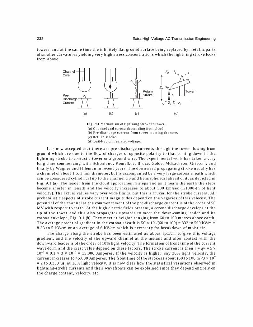
238 Extra High Voltage AC Transmission Engineering
towers, and at the same time the infinitely flat ground surface being replaced by metallic partsof smaller curvatures yielding very high stress concentrations which the lightning stroke looksfrom above.
Fig. 9.1 Mechanism of lightning stroke to tower.(a) Channel and corona descending from cloud.(b) Pre-discharge current from tower meeting the core.(c) Return stroke.(d) Build-up of insulator voltage.
It is now accepted that there are pre-discharge currents through the tower flowing fromground which are due to the flow of charges of opposite polarity to that coming down in thelightning stroke to contact a tower or a ground wire. The experimental work has taken a verylong time commencing with Schonland, Komelkov, Bruce, Golde, McEachron, Griscom, andfinally by Wagner and Hileman in recent years. The downward propagating stroke usually hasa channel of about 1 to 3 mm diameter, but is accompanied by a very large corona sheath whichcan be considered cylindrical up to the channel tip and hemispherical ahead of it, as depicted inFig. 9.1 (a). The leader from the cloud approaches in steps and as it nears the earth the stepsbecome shorter in length and the velocity increases to about 300 km/sec (1/1000-th of lightvelocity). The actual values vary over wide limits, but this is crucial for the stroke current. Allprobabilistic aspects of stroke current magnitudes depend on the vagaries of this velocity. Thepotential of the channel at the commencement of the pre-discharge current is of the order of 50MV with respect to earth. At the high electric fields present, a corona discharge develops at thetip of the tower and this also propagates upwards to meet the down-coming leader and itscorona envelope, Fig. 9.1 (b). They meet at heights ranging from 60 to 100 metres above earth.The average potential gradient in the corona sheath is 50 × 103/(60 to 100) = 833 to 500 kV/m =8.33 to 5 kV/cm or an average of 6 kV/cm which is necessary for breakdown of moist air.
The charge along the stroke has been estimated as about 5µC/cm to give this voltagegradient, and the velocity of the upward channel at the instant and after contact with thedownward leader is of the order of 10% light velocity. The formation of front time of the currentwave-form and the crest value depend on these factors. The stroke current is then i = qv = 5 ×10–6 × 0.1 × 3 × 1010 = 15,000 Amperes. If the velocity is higher, say 30% light velocity, thecurrent increases to 45,000 Amperes. The front time of the stroke is about (60 to 100 m)/3 × 107
= 2 to 3.333 µs, at 10% light velocity. It is now clear how the statistical variations observed inlightning-stroke currents and their wavefronts can be explained since they depend entirely onthe charge content, velocity, etc.
Zm
Zg
eg
ei
ic ec ic Zc
ig ig
TowerReturnStroke
( )a ( )b ( )d( )c
ChannelCore
Pre-DischargeCurrent

Lightning and Lightning Protection 239
When a stroke contacts a tower, the voltage stress experienced by the insulator is foundas follows: If Zc and Zg, Figure 9.1(d), are the surge impedances of the line conductor andground wire, and Zm the mutual impedance between them, then the ground wire and line-conductor potentials are
eg = ccgmccmgg iZiZeiZiZ +=+ and ...(9.3)where ig and ic are currents flowing from each side in the two conductors. The conductor
voltage is then
ec = cmfcgfcgmcggm iZKZeKiZZZeZZ )(.)/()/( 2 −+=−+
= cccmfgf iZZZKeK )/1(. −+ ...(9.4)where Kf = coupling factor between ground wire and conductor for a voltage applied to the
ground wire.If the surge impedances are equal, Zg = Zc, then
ec = ccfgf iZKeK )1( 2−+
The voltage across the insulator string is
ei = cccmfgfcg iZZZKeKee )/.1()1( −−−=− ...(9.5)The second term is caused by the presence of pre-discharge current contributed by the
line conductor, and if this can be artificially increased, the insulator voltage is lowered. Weobserve that ic = 0.5 ipd, where ipd = the pre-discharge current flowing in the conductor. Thesecond term gives an effective impedance of
Ze = )/1(21
cmfc ZZKZ − ...(9.6)
The reduction in insulator voltage in some designs by providing long pipes along theconductor up to 4 metres on each side has been estimated to lower the insulator voltage by15%, and the pre-discharge current measured from laboratory experiments is about 1000Amperes.
Stroke Contacting Midspan, Fig. 9.2 (a).In this case,
eg = ccgmccmgg iZiZeiZiZ +=+ and, ...(9.7)
Also, cg ii + = ,21
sI where Is = stroke current ...(9.8)
∴ Is = )/()2(2)/()(2 mgcmgcmgcg ZZiZZZZZee −−++−− ...(9.9)
Example 9.3. Taking an insulator voltage of 8000 kV, surge impedances Zg = 500, Zc =300, and Zm = 150 ohms, and the pre-discharge current ic = 15000 Amperes, calculate the strokecurrent.
Solution. Is = 2 × 8 × 106/350 + 2 × 15000× 500/350 = 46,000 + 21,400 = 67,400 Amperes
We observe that the pre-discharge current has been responsible for contributing almost33% to the intense stroke current. Photographs taken in laboratories on conductor-to-conductorgaps and on outdoor lines have shown the intense sheath of corona existing between theconductors inside which streamers are observed to propagate giving rise to such highpredischarge currents, as shown in Fig. 9.2 (b).
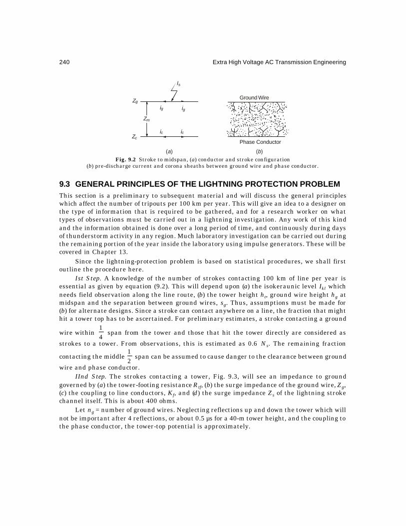
240 Extra High Voltage AC Transmission Engineering
Fig. 9.2 Stroke to midspan, (a) conductor and stroke configuration(b) pre-discharge current and corona sheaths between ground wire and phase conductor.
9.3 GENERAL PRINCIPLES OF THE LIGHTNING PROTECTION PROBLEMThis section is a preliminary to subsequent material and will discuss the general principleswhich affect the number of tripouts per 100 km per year. This will give an idea to a designer onthe type of information that is required to be gathered, and for a research worker on whattypes of observations must be carried out in a lightning investigation. Any work of this kindand the information obtained is done over a long period of time, and continuously during daysof thunderstorm activity in any region. Much laboratory investigation can be carried out duringthe remaining portion of the year inside the laboratory using impulse generators. These will becovered in Chapter 13.
Since the lightning-protection problem is based on statistical procedures, we shall firstoutline the procedure here.
Ist Step. A knowledge of the number of strokes contacting 100 km of line per year isessential as given by equation (9.2). This will depend upon (a) the isokeraunic level Ikl whichneeds field observation along the line route, (b) the tower height ht, ground wire height hg atmidspan and the separation between ground wires, sg. Thus, assumptions must be made for(b) for alternate designs. Since a stroke can contact anywhere on a line, the fraction that mighthit a tower top has to be ascertained. For preliminary estimates, a stroke contacting a ground
wire within 41
span from the tower and those that hit the tower directly are considered as
strokes to a tower. From observations, this is estimated as 0.6 Ns. The remaining fraction
contacting the middle 21
span can be assumed to cause danger to the clearance between ground
wire and phase conductor.IInd Step. The strokes contacting a tower, Fig. 9.3, will see an impedance to ground
governed by (a) the tower-footing resistance Rtf, (b) the surge impedance of the ground wire, Zg,(c) the coupling to line conductors, Kf, and (d) the surge impedance Zs of the lightning strokechannel itself. This is about 400 ohms.
Let ng = number of ground wires. Neglecting reflections up and down the tower which willnot be important after 4 reflections, or about 0.5 µs for a 40-m tower height, and the coupling tothe phase conductor, the tower-top potential is approximately.
Zm
Zg
Is
ig ig
ic icZc
( )a
Ground Wire
Phase Conductor
( )b

Lightning and Lightning Protection 241
Vt = )/1/2/1/( sggifs ZZnRI ++ ...(9.10)where the denominator is the total admittance, and Is = stroke current delivered to a
zero-impedance ground.
Fig. 9.3 Impedance presented to lightning stroke at tower.
Example 9.4. A tower has a 40-ohm footing resistance and two ground wires each with Zg
= 500 ohms. The lightning stroke surge impedance is Zs = 400 ohm. For Is = 50 kA, crest,calculate the tower top potential (a) considering all impedances, (b) neglecting the ground wireand stroke surge impedances, and (c) considering only one ground wire and stroke surgeimpedance.
Solution.
(a) Ze = 1/(1/Rtf + 4/Zg + 1/Zs) = 28.2 ohmsTherefore tower top potential Vt = 28.2 × 50 = 1410 kV, crest.
(b) Ze = Rtf = 40 ohms,∴ Vt = 2000 kV, crest(c) Ze = 1/(1/Rtf + 2/Zg + 1/Zs) = 31.75 ohms
Therefore Vt = 31.75 × 50 = 1587.3 kV, crest.
IIIrd Step. A knowledge of tower-footing resistance is therefore essential and methods forcalculation of this quantity for various types of footing arrangements such as driven rods,horizontally buried wires called counterpoises, etc., will be given in a later section.
IVth Step. When the tower-top experiences the above voltage, the insulator stringssupporting the conductors will experience a maximum voltage of
Vi = mft EKV +− )1( ...(9.11)
where Em = crest value of line-to-ground power-frequency voltage,
and Kf = coupling factor between ground wire(s) and the phase conductor.The coupling factor can be calculated from the capacitance matrix of the multi-conductor
system as shown in chapter 5, even when corona is present. The capacitance matrix is calculated
from Maxwell's Potential coefficient matrix, [c] = 10 ][2 −π Pe as shown in chapter 3. A value for
Kf = 0.2 to 0.3 is an average. Equation (9.11) is based on worst case and one must evaluate theprobability that at the instant the stroke hits the tower top the power-frequency voltage ispassing through its peak value but of opposite sign to the polarity of the lightning voltage attower top. The trip-out rate will depend on this observed probability, which is again a fieldinvestigation on an energized line in the region under consideration.
Rtf
ZgZg
ngZs
Is
242 Extra High Voltage AC Transmission Engineering
Example 9.5. A 735-kV line 3/2735( = 600 kV, crest, line-to-ground) has a couplingfactor between line and ground conductors Kf = 0.2. The tower-footing resistance is 40 ohms.Using Vt = 2000 kV crest for 50 kA lightning-stroke current, find the voltage experienced by theinsulator string.
Solution. Vi = 2000 (1 – 0.2) + 600 = 1600 + 600 = 2200 kV. We observe that the powerfrequency voltage is 600/2200 = 0.2727 or 27.27% of the insulator voltage for this example. Ifthe stroke current had been 100 kA, the reduction due to coupling to the phase conductor willbe 800 kV whereas the power-frequency voltage increases the insulator voltage to an extent of600 kV, crest. Thus, there always exist counter-balancing effects in such a game.
Vth Step. When the voltage Vi across the insulator has been estimated, we now enquire ifthis will exceed the flashover voltage of the string. For no flashover, Vi must equal the withstandvoltage of the string. Therefore, flashover and withstand voltages of insulator strings whensubjected to lightning impulses must be available from laboratory studies under all types ofatmospheric conditions. Until reflections arrive from the low towerfooting resistances at adjacenttowers to the tower hit by lightning, the insulator will be subjected to the full lightning voltage.For span length of 300 metres, a reflection arrives after 2 µs. Thus, it is essential to have the2-µs flashover data.
For standard 0143
5 ′′×" (14.6 cm × 25.4 cm) discs the average 2 µs 50% flashover values
are 125 kV per disc under dry conditions and 80 kV under rain. It is evident that the lightningvoltage must be kept below the impulse withstand voltage by a suitable margin, usually 10%.
VIth Step. The voltage experienced by the insulator is a function of the crest value oflightning-stroke current feeding into a zero-resistance ground. Therefore, the probability thatthis crest value of current will be achieved in the region where the transmission line will runmust be known in order to calculate the number of trip-outs. This is a very extensive investigationand some examples of stroke currents and their statistical occurrence will be discussed in alater section. From a large amount of data available in published literature, the author hasfound that the following expression is valid for crest currents from 25 to 70 kA with Ic inkiloamperes;
pi = 1.175 – 0.015 Ic ...(9.12)where pi = probability (fraction) of strokes having a current of crest value Ic kiloamperes.
This will also depend upon the isokeraunik level Ikl, so that a designer and research workermust obtain all the data for their region.
VIIth Step. We can now calculate the number of times in a year per 100 km of line whichwill give a voltage in excess of the flashover voltage of the insulator. This is
Nt = pi.pt.NS ...(9.13)where pi = probability that the crest value of lightning stroke current yielding the flashover
voltage of insulator will be found,pt = the fraction of strokes NS which will contact the tower.
NS = number of strokes contacting the line per year per 100 km length,
and Nt = probable number of tripouts for those strokes contacting the tower.To this must be added the number of strokes among NS that cause midspan flashover.

Lightning and Lightning Protection 243
Example 9.6. A 400-kV horizontal line has 22 discs in the insulator and two ground wiresspaced 15 metres apart at 20 m height at mid-span and 26 m at the tower. The tower-footingresistance is 40 ohms. The surge impedances are: Ground wire: 500 ohms, stroke: 400 ohms.
Assume 60% of strokes to contact within 41
span of line from the tower and at the tower top.
The coupling factor between ground and phase conductor is 0.2 and the factor in NS is 0.2. Theisokeraunik level is 60 thunderstorm days per year. Calculate the number of tripouts per yearper 100 km of line. See Fig. 9.3.
Solution.
(1) From equation (9.2),
NS = 0.2 × 60 0.0133 (26 + 2 × 20) + 0.1 × 15
= 29.6 strokes/100 km-year.
(2) From equation (9.10),
Vt = Is/(1/Rtf + 4/Zg + 1/Zs) = 28.2 Is, kV, with the stroke current Is in kA.(3) From equation (9.11),
Vi = (1 – 0.2) Vt + 400 3/2 = 22.56 Is + 326, kV, crest
(4) Flashover voltage of 22 discs = 22 × 125 = 2750 kV in fair weather. In rain, flashovervoltage = 1760 kV.
(5) Therefore 2750 = 22.56 Is + 326, which gives the stroke current to beIs = (2750 – 326)/22.56 = 107.4 kA.
In rainy weather , Is = (1760 – 326)/22.56 = 63.6 kA.(6) The probability of reaching these crest currents are:
In rain : pi = 1.175 – 0.015 × 63.6 = 0.221.In fair weather: The value of 107.4 kA is beyond the range of equation (9.12). Butfrom Fig. 9.5, it is pi = 0.04.
(7) Using values under rainy conditions, the number of probable tripouts is, from equation(9.13),
Nt = 0.22 × 0.6 × 29.6 = 3.925 per 100 km/yearUsing dry-weather values,
Nt = 0.04 × 0.6 × 29.6 = 0.7 per 100 km/yearWe shall now discuss all the factors involved in the estimation of tripouts in some detail in
the following sections.
9.4 TOWER-FOOTING RESISTANCEThe tower-footing resistance Rtf will depend on (a) the type of electrode configuration employed,and (b) the soil resistivity. The most common types of electrode shapes are (1) the hemisphere,(2) long slender rods of about 2 to 5 cm diameter and 10 to 15 metres in length driven verticallydown into the soil and connected to tower legs, and (3) buried horizontal wires called the'counterpoise' of 50 to 150 metres in length in soil where vertical rods cannot be driven. In allcases, sufficient area must be exposed between the electrode and soil in order for the current tospread over a large area.

244 Extra High Voltage AC Transmission Engineering
Soil resistivities, sρ , have the following ranges:
Sea Water Moist Soil Loose Soil and Clay Rock100 101 102 > 103 ohm-metre
The electrode shapes and their dimensions are shown in Fig. 9.4 and the formulae forresistances of various types of electrodes are given in the following table.
Electrode Shape Resistance
(1) Hemisphere, R Rs πρ 2/
(2) Vertical driven rod
−
πρ
πρ
14
ln2
,or),/2ln(2 a
ll
all
ss
(radius a, length 2l) (Rudenberg) = )Dwight()/472.1ln(2
all
s
πρ
.
(3) Horizontal wire.
+
πρ
)/2ln()/ln(
1)./2ln(2 al
ylal
ls
(radius a, length 2l, depth y) )/2ln()2/( 2 aylls πρ=
Fig. 9.4 Tower-footing electrodes. Hemisphere, driven rod and buried counterpoise.
Example 9.7. It is necessary to obtain a tower-footing resistance of 20 ohms in a soil ofresistivity sρ = 100 ohm-m using the three different types of electrodes shown above. Take a =1.25 cm for rods and counterpoises and a depth y = 0.5 m for the counterpoise. Calculate therequired dimensions.
Solution.
(1) Hemisphere. R = metre8.0202/1002/ =×π=πρ tfs R(2) Vertical Driven Rod. The equation to be solved for l is
ln (2l/0.0125) = 2πl × 20/100 = 0.4πl.Trial and error gives l = 5.4 metres.
(3) Horizontal Counterpoise. The equation isln (2l2/0.0125 × 0.5) = ln (320l2) = 0.4πl.This gives l = 8 metres.
In the case of driven rods and counterpoises, the resistance is distributed along theirlengths and the current entering them will exhibit travelling-wave effect with the result that
Rρs
Hemisphere
ρs
2a
Vertical Driven Rod
2l
ρs
2l
y
2a
HorizontalBuried WireCounterpoise

Lightning and Lightning Protection 245
initially the surge current will see the surge impedance but after a few reflections the resistanceassumes the values given above. Usually 4 reflections are sufficient to change the resistancefrom the surge impedance to the steady value.
9.5 INSULATOR FLASHOVER AND WITHSTAND VOLTAGES
Under positive polarity lightning impulses, a standard "" 1043
5 × disc (14.6 cm × 25.4 cm) shows
a highly linear characteristic between spark-over voltage and number of discs. In fair or dryweather conditions, they can be expressed by the following values:
Time to Breakdown, µs 0.5 1.0 2.0 3.0 4.0 6.0 8.0kV/disc, crest 188 150 125 110 105 97.5 92.51.20/50 µs wave, kV/disc = 87.5 kV crestPower Frequency. In fair weather the flashover voltage is 75 kV/disc, crest value, or 53
kV/disc, r.m.s. value. A standard disc has leakage distance of 31.8 cm (12.5 inches) over itssurface. The usual creepage strength used is 1 kV/cm of leakage distance, r.m.s. value.
Strings in Parallel. When lightning hits a line, many insulators are stressed in parallel. Ithas been found in practice from outdoor experiments that under lightning-type of voltage withextremely small wave-front (1 – 2µs), this point is not important as it definitely is under longersurges such as the switching surge. Therefore, single-string values for voltage can be used forflashover and withstand strength.
Conductor-conductor Flashover. Under positive lightning wave the following empiricalrelation based upon experimental work can be taken:
Flashover voltage Vcc = 590 kV/metre, crest
9.6 PROBABILITY OF OCCURRENCE OF LIGHTNING STROKE CURRENTS
The probability or the fraction of strokes reaching the ground whose magnitude is above a givenanticipated value must be ascertained for the region in which the line will be run. Such experimentsuse 'magnetic links' connected near tower tops and conductors whose magnetization intensitywill depend upon the crest value of current. A typical probability curve is presented in Fig. 9.5.
Fig. 9.5 Probability of occurrence of stroke-current magnitudes.
00 20 40 60 80 100 120 140 kA
0.2
0.4
0.6
0.8
1.0
Peak Impulse Current
Probability

246 Extra High Voltage AC Transmission Engineering
9.7 LIGHTNING ARRESTERS AND PROTECTIVE CHARACTERISTICSLightning arresters, also called 'surge absorbers' because they are also meant for switching-surge protection, protect primarily major equipment such as transformers, rotating machines,shunt reactors, and even entire substations. Less expensive protective devices such as rod gapscan be used for protection of transformer and circuit-breaker bushings and open contacts.When substations have to be protected, they are located at the entrance of the incoming andoutgoing lines. Modern surge absorbers for e.h.v. levels are designed to offer protection toequipment and lines for both lightning overvoltages and currents as well as switching surgeover-voltages where the energy involved is much higher. Their characteristics will be describedlater. Arresters are of three important types and classified according to their internal structure.They are
(1) Gap type arrester without current-limiting functions;(2) Gap type arrester with current-limiting capability; and(3) Gapless metal oxide varistors.The first is commonly known by trade names such as Thyrite, Magnavalve, Autovalve,
Miurite, etc., each one being associated with its manufacturer. The non-linear resistance materialis usually sintered Silicon-Carbide (SiC) and is designed to dissipate the energy in short durationlightning-stroke current and the current at power frequency that will follow this current whenthe series gap conducts. The current is finally interrupted at a power-frequency zero. Thesecond, or the current-limiting gap type, is of North-American and European design in which amagnetic action on the arc between the gap creates a lengthening of the arc with consequentlarge resistance capable of limiting the current. In such a design, the power-frequency currentcan be extinguished prior to reaching a current zero. Such an arrester can perform switching-surge duty also. The non-linear resistance is still SiC. The last one, the gapless MOV, is ofrecent origin, having been patented only in 1968 by a Japanese firm for low-voltage low-currentelectronic circuitary but now is sufficiently well developed to handle e.h.v. requirements.
Protective Ratio . The most important property of a surge absorber is the 'protective ratio'which is defined as
Np = value R.M.S. Voltage,frequency -PowerArrester RatedEquipment Protected of Level Insulation ImpulsePeak
Typical examples of lightning arrester protective ratios are given in Table 9.1.The selection of an arrester with a specified voltage rating is governed by the value of
'earthing coefficient' or the 'earth-fault factor'. These are defined as follows and are based on asingle line to ground fault conditon.
EC = locationarrester at voltage line-to-Linelocationarrester at voltage phasehealthy of Value RMS
...(9.14)
The earth-fault factor, EFF = EC×3 ...(9.15)and uses the line-to-ground voltage in the denominator of equation (9.14). The Indian standardsand the I.E.C. use the EFF but arresters are still known by the earthing coefficient value.Thus, on a 400-kV line with a maximum operating voltage of 420 kV, an 80% arrester has a
rating of 336 kV, r.m.s. with EC = 0.8 and EFF = 38.0 .
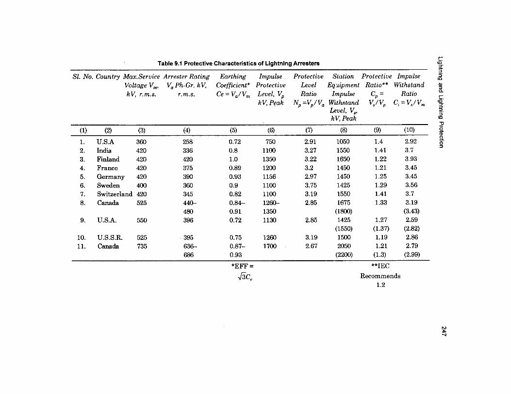

248 Extra High Voltage AC Transmission Engineering
Under a single line to ground fault, the voltage of the faulted phase is zero at the faultwhile the voltages of the remaining two healthy phases will rise above normal working voltage.The lightning arrester must withstand this higher voltage without sparkover of the series gapnor conduct current in a gapless arrester. The calculation of earthing coefficient is discussed insection 9.8. In Table 9.1, column 5 shows values of EC used in various countries which haveranged from a low value of 0.72 in the U.S.A. with solidly-earthed neutrals of equipment to ahigh of 1.0 in Finland using isolated-neutral system (tuned coil).
Discharge Current. The second important quantity for the arrester selection is the lightning-type impulse current which the arrester material has to discharge without damage to itself.Representative values of standard 8/20 µs surge currents taken from IS 3070 (Part I)— 1974are given below:
Crest 8/20 µs current, Amps 5000 10000 15000 20000System voltage, kV up to 230 345–400 500 750 (735–765)Protective Level. The third important characteristic of an arrester is the protective level
offered by it to the connected equipment. Having selected the arrester rating based on thesystem earthing coefficient for a bus fault, the manufacturer of the arresters can provide aresistance material which has a specified I-V characteristic. In ideal cases, the voltage acrossthe arrester material should be constant for all current values which flow through it. In a gap-type arrester there is the additional quantity, the sparkover voltage. When the gap sparksover, the lightning current is drained to ground through the arrester material. This will holdan IR-voltage which depends on the non-linear resistance characteristic of the SiC material.The protective level offered by a lightning arrester is the higher of the following two voltagevalues:
(1) Sparkover voltage of the series gap under a standard 1.2/50 µs impulse; or
(2) Residual voltage (the IR-drop) when discharging the specified test impulse current of8/20µs waveshape. For gapless arresters only item (2) applies.
With the constant improvements taking place in arrester material and voltage-control(grading) circuits incorporated in the arrester chamber, the above two values are made nearlyequal. Table 9.2 gives representative values. In older types (before 1970) the 250/2500 µsswitching-surge spark-over voltage was taken as 83% of the short-duration steep-front lightning-impulse breakdown. But in modern arresters, the two are made nearly equal by proper voltagecontrol circuitry.
Table 9.2 Lightning Arrester Sparkover–Discharge Voltage Characteristics
System Maximum Arrester Rating, 1.2/50µs Discharge Switching SurgeContinuous Oper- kV, RMS Sparkover Voltage, kV. Sparkover kV,ating Voltage, kV kV, crest 8/20µs, kA crest
362 258 (72%) 625 585 610276 (76%) 670 625 10 650312 (86%) 770 705 735
550 372 (68%) 895 905 870396 (72%) 955 965 15 925420 (76%) 1010 1020 980
800 540 (67.5%) 1300 1390 1200576 (72%) 1400 1500 20 1285612 (76%) 1465 1580 1370

Lightning and Lightning Protection 249
When current-limiting gap-type arresters were not used, the power-follow current flowingdue to 50 Hz voltage when the gap has sparked over had to wait until a current zero, in orderthat the current through the arrester resistor material could be interrupted, as it does in acircuit breaker. However, in modern current-limiting arresters, the arc can be elongated toany desired extent in a suitably-designed arcing chamber to interrupt the current very quicklywithout waiting for a current zero. This reduces the energy dissipated by the SiC material andthe performance is improved considerably even under switching-surge conditions when theenergy discharged by a long transmission line could be considerable.
The lower the protective level offered by the arrester, it is evident that lower can be theinsulation level of the equipment it protects. This will bring down the cost of major equipmentsuch as transformers. Examples are already provided in Table 9.1. According to IS 2026 : PartIII (1981) examples of equipment insulation levels are given in Table 9.3 below:
Table 9.3 Lightning Arrester Protective Levels and Equipment Insulation(Transformers)
Nominal Highest Rated Switching Rated Lightning L.A.System Equipment Impulse withstand Impulse Withstand Protective
kV, RMS Voltage, kV (Phase-Neutral) Voltage, kV crest Level,RMS kV, crest kV, crest
275 300 750 850 and 950850 950 and 1050
345 362 850 950 and 1050 625-770950 1050 and 1175
400 420 950 1050 and 11751050 1175, 1300 and 1425
500 525 1050 1175, 1300 and 1425 895-10101175 1425 and 1550 1010
750 765 1425 1550 and 1800 1300-14651550 1800 and 1950
The ideas discussed above can be represented pictorially as shown in Figure 9.6.
Fig. 9.6 Pictorial representation of arrester voltage rating, earthing coefficient Ce overvoltageunder lightning and switching impulses, protective level of arrester, and margins.
P.U.
0
1
2
3
4 1.2/50 sµ
250/2500 sµ Withstand
V = Ce Va m3V , L – Nm
System Voltages
Lightning
Switching Margins
Vp
Vq
Arrester Characteristics
VCV
aem
= Arrester Rating = Earthing Coefficient = Rated Peak
Vp = Protective Level
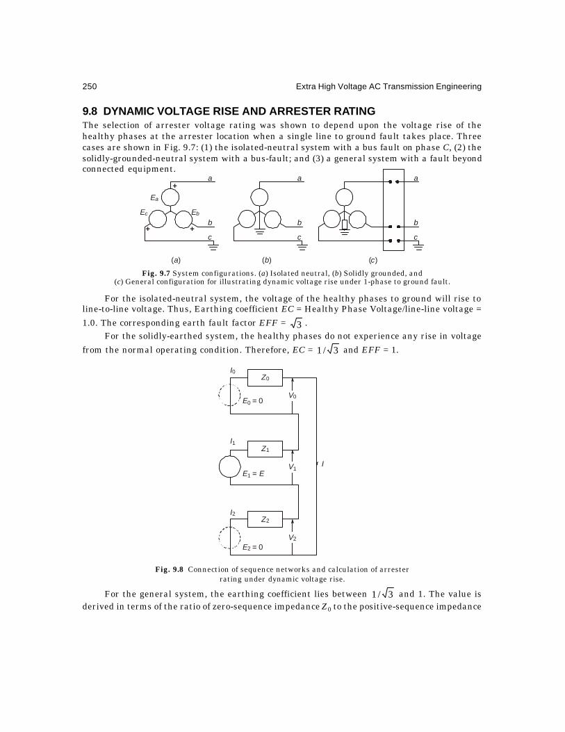
250 Extra High Voltage AC Transmission Engineering
9.8 DYNAMIC VOLTAGE RISE AND ARRESTER RATINGThe selection of arrester voltage rating was shown to depend upon the voltage rise of thehealthy phases at the arrester location when a single line to ground fault takes place. Threecases are shown in Fig. 9.7: (1) the isolated-neutral system with a bus fault on phase C, (2) thesolidly-grounded-neutral system with a bus-fault; and (3) a general system with a fault beyondconnected equipment.
Fig. 9.7 System configurations. (a) Isolated neutral, (b) Solidly grounded, and(c) General configuration for illustrating dynamic voltage rise under 1-phase to ground fault.
For the isolated-neutral system, the voltage of the healthy phases to ground will rise toline-to-line voltage. Thus, Earthing coefficient EC = Healthy Phase Voltage/line-line voltage =
1.0. The corresponding earth fault factor EFF = 3 .For the solidly-earthed system, the healthy phases do not experience any rise in voltage
from the normal operating condition. Therefore, EC = 3/1 and EFF = 1.
Fig. 9.8 Connection of sequence networks and calculation of arresterrating under dynamic voltage rise.
For the general system, the earthing coefficient lies between 3/1 and 1. The value isderived in terms of the ratio of zero-sequence impedance Z0 to the positive-sequence impedance
V0
V1
V2
E0 = 0
E E1 =
E2 = 0
I0
I1
I2
I
Z0
Z1
Z2
a a a
b b b
c c c
+
+ +
Ea
Ec Eb
( )a ( )b ( )c

Lightning and Lightning Protection 251
Z1 up to the fault. When single line to ground fault occurs, according to symmetrical-componenttheory, the three sequence networks are connected in series, as shown in Fig. 9.8. Only thepositive-sequence network contains a driving voltage E. The current is
I = )(/ 210 ZZZE ++ ...(9.16)
∴ The three sequence voltages at the fault are
V0 = )//1/( 020100 ZZZZEIZE ++−=− ...(9.17)
V1 = )//1/( 121011 ZZZZEEIZE ++−=− ...(9.18)
and V2 = )//1/( 212022 ZZZZEIZE ++−=− ...(9.19)
For static equipment such as lines and transformers, Z1 = Z2. Let, up to the fault,m = Z0/Z1 = zero-sequence impedance/positive-sequence impedance.
Then, V0/E = )2/()1(/),2/( 1 ++=+− mmEVmm
and V2/E = –1/(m + 2) ...(9.20)The healthy phase voltage such as Vb is with a = °∠1201 ,
EVb =
EaVVaV ++ 1
20
=2
)866.05.()1)(866.05.0(+
+−−+−−+−m
jmjm
and its p.u. value is
EVb =
21
32
+++
mmm
, when m is real quantity. ...(9.21)
This will apply when R0 /x0 = R1/x1, where R and x are the resistance and reactancecomponents of Z. The earthing coefficient is therefore
EC = ,0,2
1
3
2
≠+
++= mm
mm
E
Vb
When m varies from 1 to ∞ , the earthing coefficient and earth fault factors have thefollowing values.
m = Z0/Z1 1 2 2.5 3 3.5 4 5 7.5 10 ∞EC 0.578 0.66 0.7 0.721 0.744 0.764 0.795 0.849 0.88 1
EFF 1 1.14 1.20 1.25 1.29 1.323 1.38 1.47 1.52 3
9.9 OPERATING CHARACTERISTICS OF LIGHTNING ARRESTERSIn this section we will describe the three types of arresters used in e.h.v. systems in detail.These are (1) the gap-type SiC arrester, (2) the current-limiting gap-type SiC arrester, and (3)the gapless metal oxide varistor or the zinc-oxide (ZnO) arrester.

252 Extra High Voltage AC Transmission Engineering
9.9.1 Gap Type SiC ArrestersIn both the non current-limiting and current-limiting types, the material is sintered SiliconCarbide which is made for a voltage rating of 6 kV, r.m.s., per disc. As many discs as arenecessary for the arrester rated voltage are stacked in series and provided with voltage-gradingcircuits. These may consist of high voltage resistors, capacitors, or a combination of both. TheI-V characteristics of both types are shown in Fig. 9.9. They function in two stages: (a) Uponoccurrence of an overvoltage, the gaps sparkover and provide a low-impedance path to ground.(b) The series resistor reduces power-frequency follow current so that the arc across the gap isable to re-seal either before or at the following voltage and current zero. In the magnetically-blown-out surge arrester, Fig. 9.9(b), the arc is lengthened so that the resulting back e.m.f.helps to reduce the power follow current. The energy loading is about 7 kJ/kV during limitingswitching surges with a protection level of 2.2 p.u. being attained.
Fig. 9.9 I-V characteristics of (a) gap-type non current-limiting type, (b) gap-type current-limiting type,arresters. (c) Time lag of breakdown of series gap with voltage-grading circuits.
The resistance of a valve element is non-linear with 8.5 kV crest )26( for 1250 Amperesand only 12 kV crest for 10,000 Amperes surge current. These values give an I-V relations.
V = 2604 I0.166 (or 6VI ∝ ) ...(9.21)
where V and I are in volts and amperes. The resulting resistance is
R = 834.02604/ −= IIV ohms. ...(9.22)Ideally, if the material is to hold a constant value of voltage at all currents, the resistance
of the material must vary as 1. −= IKR idid . This is nearly fulfilled in Metal Oxide Varistors,but not in a SiC arrester.
In a non current-limiting arrester, the gap breaks down on the incidence of a lightningovervoltage, which is set at a power-frequency voltage of 1.5 to 2.0 p. u. and at a lightningvoltage equal to the protective level. In addition to the lightning current of standard wave-shape of 8/20 µs, the material conducts the power-follow current with a very large dissipation ofheat in the resistor. In addition, under a switching surge discharge, currents are high and theduration can be as much as 2000 µs. Therefore, lightning arresters are subjected to 3 types oftests:
(1) The power-frequency flashover of the gap. This should not take place for 1 minute atless than 1.5 p. u. voltage [With an earthing coefficient of 0.8 say, the arrester ratedvoltage is 0.8 3 = 1.3856 times the maximum line-to-neutral operating voltage].
V
VS
VN
INormal Gap
Type SiC( )a
V
VS
VN
ICurrent Limiting Gap
Type SiC( )b
Time to Sparkover
( )c
1 10 102 103 µs
2
V VA N/

Lightning and Lightning Protection 253
(2) An 8/20 µs standard lightning impulse current test. The resulting voltage must notexceed the protective level offered by the arrester at rated currents of 5, 10, 15 or 20kiloamperes, crest. The protective level is given in Table 9.3.
(3) A long-duration current test of 100-150 Amperes of 1000 µs duration. This simulatesswitching-surge duty when a line is energized from a source.
By using a suitably-designed grading network to control the distribution of voltage amongstthe series-connected gaps, the voltage-time characteristic of the arrester is controlled muchbetter than without them as shown in Figue 9.9(c).
9.9.2 The Gapless Metal Oxide ArresterRecent advances in solid-state physics in electronics have been applied to develop a materialwhich is ideal for surge arrester. SiC resistors have a characteristic I = KVα , with α = 4 to 6.This is not high enough for arresters without spark gaps. A ceramic material based on oxides ofZn, Bi, and Co has α > 20 and can handle a very large current range. The I-V characteristic isnearly ideal with a constant protective level from a few milliamperes to thousands of amperesover a 5 decade range. The base material is ZnO (n-material) grains sintered in a flux of variousinsulating oxides such as Bi2O3. Other constituents are CoO, MnO and Cr2O3. These changeenergy levels and hence the conduction and insulating properties. These oxides coat the high-conductivity ZnO grains with a thin insulating layer of 100-200
oA as shown in Fig. 9.10. The
resulting I-V characteristic is nearly 5035−∝ VI .
Example 9.8. Two arrester materials have the characteristics 6VI ∝ and 40VI ∝ . Forcurrent variations from 10 Amperes to 100,000 Amps., determine the ratio of voltages at thesecurrents.
Solution. (a) 10 = 62
561 10and KVKV =
∴ 645.410)10(/ 667.06/1412 ===VV
(b) 10 = 402
5401 10and KVKV =
∴ V2/V1 = (104)1/40 = 100.1 = 1.26.
Fig. 9.10 Internal structure and external I-V characteristics of ZnO gapless arrester.Comparison with SiC arrester.
Therefore, higher the index of V, the less is the rise in voltage and more it approaches theideal. A comparison of gap-type SiC arrester and gapless ZnO arrester is shown in Fig. 9.10(c).ZnO arresters are usually made in discs of 80 mm diameter and 32 mm thickness. At the
V
VpZnO
SiC
I( )c( ) Idealb( ) Reala
ZnO grain
Contacts
CurrentLoads
IntermediateInsulation Layer
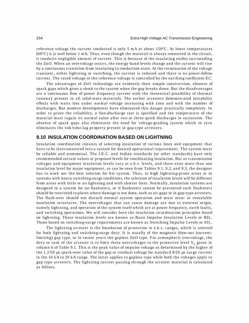
254 Extra High Voltage AC Transmission Engineering
reference voltage the current conducted is only 5 mA at about 150°C. At lower temperatures(60°C) it is well below 1 mA. Thus, even though the material is always connected in the circuit,it conducts negligible amount of current. This is because of the insulating oxides surroundingthe ZnO. When an overvoltage occurs, the energy band levels change and the current will riseby a continuous transition from insulating to conduction state. At the termination of the voltagetransient, either lightning or switching, the current is reduced and there is no power-followcurrent. The rated voltage or the reference voltage is controlled by the earthing coefficient EC.
The advantages of ZnO technology are evidently their simple construction, absence ofspark gaps which gives a shock to the system when the gap breaks down. But the disadvantagesare a continuous flow of power frequency current with the theoretical possibility of thermalrunaway present in all solid-state materials. The earlier arresters demonstrated instabilityeffects with watts loss under normal voltage increasing with time and with the number ofdischarges. But modern developments have eliminated this danger practically completely. Inorder to prove the reliability, a line-discharge test is specified and the temperature of thematerial must regain its normal value after two or three quick discharges in succession. Theabsence of spark gaps also eliminates the need for voltage-grading system which in turneliminates the volt/time-lag property present in gap-type arresters.
9.10 INSULATION COORDINATION BASED ON LIGHTNINGInsulation coordination consists of selecting insulation of various lines and equipment thathave to be interconnected into a system for desired operational requirement. The system mustbe reliable and economical. The I.E.C. and Indian standards (or other standards) have onlyrecommended certain values or proposed levels for coordinating insulation. But as transmissionvoltages and equipment insulation levels vary at e.h.v. levels, and there exist more than oneinsulation level for major equipment, as can be seen from Tables 9.1, 9.2, and 9.3, the designerhas to work out the best solution for his system. Thus, in high lightning-prone areas or insystems with heavy switching-surge conditions, the selection of insulation levels will be differentfrom areas with little or no lightning and with shorter lines. Normally, insulation systems aredesigned in a system for no flashovers, or if flashovers cannot be prevented such flashoversshould be restricted to places where damage is not done, such as air gaps or in gap-type arresters.The flash-over should not disturb normal system operation and must occur in resealableinsulation structures. The overvoltages that can cause damage are due to external origin,namely lightning, and operation of the system itself which are at power frequency, earth faults,and switching operations. We will consider here the insulation co-ordination principles basedon lightning. These insulation levels are known as Basic Impulse Insulation Levels or BIL.Those based on switching-surge requirements are known as Switching Impulse Levels or SIL.
The lightning arrester is the foundation of protection in e.h.v. ranges, which is selectedfor both lightning and switching-surge duty. It is usually of the magnetic blow-out (current-limiting) gap type, or in recent years the gapless ZnO type. For atmospheric overvoltage, theduty or task of the arrester is to limit these overvoltages to the protective level Vp given incolumn 6 of Table 9.1. This is the peak value of impulse voltage as determined by the higher ofthe 1.2/50 µs spark-over value of the gap or residual voltage for standard 8/20 µs surge currentin the 10 kA to 20 kA range. The latter applies to gapless type while both the voltages apply togap type arresters. The lightning current passing through the arrester material is calculatedas follows.

Lightning and Lightning Protection 255
Consider a travelling wave of voltage Vw, crest, which is accompanied by a current wave Iwon a line with surge impedance Z, Fig. 9.11. They strike an arrester whose duty is to hold thevoltage across it constant at the protective level Vp. Now, by using Thevenin's theorem, withthe arrester terminals open, the incident travelling wave will give a voltage 2Vw due to totalreflection. The Thevenin impedance looking through the open arrester terminals is equal tothe surge impedance Z of the line.
Fig. 9.11 Calculation of arrester current.
Fig. 9.12 Sphere-to-plane and rod-to-plane protective gaps for insulationcoordination of equipment.
Therefore, with the arrester connected, the current through it will beIa = (2Vw – Vp)/Z ...(9.23)
The maximum value the travelling-wave voltage Vw can reach is the flashover voltage ofthe line insulation. Also, it is assumed that Vp stays fairly constant at all current values dischargedby the arrester.
Example 9.9. For a 750 kV line, take Vw = 3000 kV, crest, travelling on the line and Vp =1700 kV. The line surge impedance is Z = 300 ohms. Calculate and discuss (a) the currentflowing in the line before reaching the arrester, (b) the current through the arrester, and(c) the value of arrester resistance for this condition and verify the reflection and refractioncoefficients giving rise to the voltage and current conditions.
Solution.
(a) Iw = ZVw / = 3000/300 = 10 kiloamperes.
(b) Ia = ZVV pw /)2( − = (6000 – 1700)/300 = 14.33 kA.
(c) The reflected current in the line is + 4.33 kA.This gives rise to a reflected voltage of – 4.33 × 300 = – 1300 kV. Under these conditions,
the arrester resistance isRa = Vp/Ia = 1700 kV/14.33 kA ≈ 120 ohms. (118.6 ohms).
VW, IWVp
Ia
Z
R
g

256 Extra High Voltage AC Transmission Engineering
With the line surge impedance Z = 300 ohms, the following reflection and refractioncoefficients are found.
(1) Voltage reflection factor : Kr = 73
300120300120
−=+−
=+−
ZRZR
a
a
∴ Reflected voltage Vr = Kr.Vw = – 3 × 3000/7 = – 1300 kV.(2) Voltage refraction factor : Kt = 2Ra/(Ra + Z) = 1 + Kr = +4/7.∴ Junction voltage at arrester, Vp = KtVw = 1700 kV.(3) Current reflection factor : Jr = (Z – Ra)/(Z + Ra) = – Kr = + 3/7.∴ Reflected current Ir = JrIw = + 4.33 kA(4) Current transmission factor : Jt = 2Z/(Z + Ra) = + 10/7∴ Arrester discharge current Ia = JtIw = 14.33 kA.This example shows that for such a 750 kV line an arrester rated for 15 kA would be
necessary. U sually a 750-kV line will be equipped with about 35 standard "" 1043
5 × insulator
discs whose withstand value is about 3000 kV.The protective ratio can be calculated if the rated voltage of the arrester is known from
the system conditions.
Example 9.10. For the above example , if an 80% arrester is used, calculate the protectiveratio Np = Vp/Va.
Solution. For rated line-to-line voltage of 750 kV, arrester rating isVa = 0.8 × 750 = 600 kV (R.M.S.).
∴ Protective ratio Np = 1700/600 = 2.83.Voltage Across Equipment Protected by ArresterIn the ideal case, the arrester must be located adjacent to the equipment which is usually
a large transformer or shunt reactor. In practice, however, there may be a length of the linebetween the two extending to 20 to 40 metres. This results in a slightly higher voltage acrossthe equipment due to repeated reflections. The high inductance of a transformer or reactorrepresents nearly an open-circuit to a surge. The excess voltage experienced is given by anempirical equation and depends on the line length and the rate of rise of the voltage, thus:
V∆ = (dVw /dt). (l/150)kV, ...(9.24)
where l = length of line in metresand dVw /dt = steepness of wave front in kV/µs of the incoming wave. This can be
taken as approximately 500 kV/µs for lines with overhead ground wiresand 1000 kV/µs when a line conductor is hit. (A line without earthwires).
Example 9.11. A transformer is connected by a length of 20 metres of line to an arrester.The rate of rise of voltage is 700 kV/µs. The arrester voltage is 1700 kV. Calculate the voltageacross the transformer.
Solution. V∆ = (700) × (20/150) = 93 kV.
∴ Transformer voltage = 1793 kV, impulse crest.

Lightning and Lightning Protection 257
Note that from Table 9.3, for 750 kV system voltage, the transformer lightning-impulsewithstand voltages have levels ranging from 1550 to 1950 kV.
The transformer insulation level is kept higher than the arrester protective level by asafe margin as shown by column 8 of Table 9.1. The I.E.C. suggests a value of 1.2 Vp as theequipment insulation level. This is the protective ratio Cp = Vs/Vp, where Vs = voltage level ofstation equipment insulation. It depends on the earthing coefficient, Ce, the impulse protectivelevel ratio of arrester, Cp, and the impulse protective ratio of equipment, Ci. Thus, the equipmentinsulation level is
Vs = Ce.Cp.Ci.Vwhere V = rated r.m.s. value of power-frequency line-line voltage of the system.
Example 9.12. For a 750-kV system with maximum operating voltage of 765 kV at thereceiving-end substation, the earthing coefficient is Ce = 0.84, the protective level ratio of thearrester is 2.83, and the equipment insulation level ratio is 1.3. Calculate the impulse withstandvoltage of the equipment insulation.
Solution. Vs = 0.84 × 2.83 × 1.3 V = 3.094 × 765= 2370 kV, crest.
[Note. I.E.C. suggests a 2400 kV level. But this has not yet found acceptance as a standard].
Example 9.13. For a 400-kV system (420 kV maximum) the impulse level of a transformeris 1425 kV, crest or peak. Calculate the ratio of impulse withstand level of transformer insulationto the maximum service voltage.
Solution. Ct = Ce.Cp.Ci = Vs/V = 1425/420 = 3.4Rod-Plane Spark GapThus far, the requirement and protection afforded by a lightning arrester were discussed.
For providing further safety to major equipment insulation in transformers, reactors and circuitbreakers as well as their bushings, rod-plane and rod-rod gaps will normally be used in parallel,which are variously known as protective gaps or spill gaps. These have a time lag of sparkoverranging from 2-10 µs depending upon the gap length between electrodes so that the protectedequipment must be capable of withstanding the flashover voltage of the gaps for this length oftime.
Average 50% flashover voltage values of rod-plane and rod-rod gaps are given by well-known formulas, which are on the average as follows, with d in metres:
Electrode Power Frequency Lightning ImpulseGeometry kV crest kV crestRod-Plane V50 = 652.d0.576 500 dRod-Rod V50 = 850 d0.576 650 d
The withstand value for these gaps is normally 85% of the 50% flashover voltage.Characteristics of 50% flashover and withstand voltages of long air gaps will be discussed inChapter 11.
Example 9.14. A 750 kV bushing is protected by gaps which withstand 2 p.u. power-frequency voltage. Determine their 50% flashover value under 50 Hz and lightning-impulsevoltages, if (a) rod-plane gap is used, and (b) rod-rod gap is used.

258 Extra High Voltage AC Transmission Engineering
Solution. The calculation will be based on the power-frequency voltage of 750 kV, r.m.s.,line-line. The 1 p.u. line-to-ground crest value is
3/2750 = 612 kV.∴ 2 p.u. = 1224 kV, which is the withstand voltage, Vw,The flashover value is taken to be V50 = Vw/0.85 = 1440 kV.
(a) For a rod-plane gap, d = 736.1576.0/150 2086.2)652/( =V
= 3.958 metres.For this gap length, the lightning-impulse 50% flashover value is V50 = 500 d = 1980 kV,
crest. The withstand voltage will be approximately 85% of this value, or Vwi = 0.85 × 1980 =1683 kV, crest.
(b) For a rod-rod gap d = (1440/850)1.736 = 2.5 metres. The 50% flashover under lightningimpulse voltage is
V50 = 650 d = 1625 kV, crestand the impulse withstand is Vwi = 0.85 × 1625 = 1381 kV, crest.For adequate protection and proper insulation coordination, the protective gap flashover
values must be higher than the lightning arrester protective voltage level and lower than thetransformer or bushing insulation levels.
Review Questions and Problems
1. A region has 75 thunderstorm days in a year. A 400-kV line has a tower height of 35m with two ground wires at 25 metre height at midspan and separated by 20 metres.What is the probable number of strokes contacting 400 km of line per year?
2. Describe with neat sketches the machanism of lightning stroke contacting (a) a tower,and (b) midspan.
3. A 750-kV horizontal line has 35 discs in the insulator. The two ground wires arespaced 30 m apart at heights of 30 metres at midspan and 40 metres at the tower. Thetower-footing resistance is 20 ohms. The coupling factor between a ground wire andphase conductor is 0.15 and the factor in NS is 0.2 for calculating number of strokescontacting the line per 100 km in a year. The isokeraunik level is 100 days per year.Assume 50% of strokes to contact the tower. Calculate the stroke current to flashoverthe insulator string if the surge impedance of stroke is 400 ohms, and groundwiresurge impedance is 500 ohms. Take the flashover value of one disc as 125 kV, peak,for lightning impulse.
4. Define the terms (a) earthing coefficient, (b) earth fault factor, (c) residual voltage, (d)arrester rating, and (e) insulation co-ordination.
5. Compare the performance characteristics of Silicon Carbide arrester with a Zinc Oxidearrester. What are the advantages and disadvantages of each?
6. A voltage wave of 2500 kV is travelling on a line of surge impedance 275 ohms. Thearrester connected to the line has a protective level of 1500 kV. Calculate (a) thecurrent in the wave, (b) the curent through the arrester, and (c) the arrester resistanceat this current.

10.1 ORIGIN OF OVERVOLTAGES AND THEIR TYPESOvervoltages due to the release of internally trapped electromagnetic and electrostatic energyin an e.h.v. system cause serious damages to equipment insulation. These could, under manycircumstances, be more severe than lightning damage which we considered in the previouschapter. Surge diverters and resistances included purposely while making switching operationsas well as other schemes reduce the danger to a considerable extent. This chapter will describeall these schemes and discuss the equations that indicate overvoltages and the background forsuggested remedies. Investigation of switching overvoltages has assumed very great importanceas transmission voltages are on the increase and line lengths and capacity of generating stationsare also increased. The short-circuit capacity of sources is responsible for a large amount ofdamage to insulation.
Overcurrents are generated by short circuits and lightning, but they do not form thesubject matter of this chapter. The problems of calculating short-circuit currents fromsymmetrical-component theory are well covered in a large number of treatises. Here, some ofthe overvoltage conditions caused by interruption of short-circuit currents will only be discussedwith due regard to the duty imposed on the circuit breaker through the restriking and recoveryvoltages. They bring in the concept of terminal fault, short-line fault, two-and four-parameterrepresentations of the recovery voltage. In addition, interruption by the circuit breaker of lowinductive currents such as dropping transformers and shunt reactors cause overvoltages becauseof sudden collapse of current described by the phenomenon of ‘current chopping’. Interruptionof small capacitive currents caused by dropping an unloaded line bring over-voltages because ofpossibility of re-striking in the arcing chamber of the breaker. Ferro-resonance conditionsexist when the circuit-breaker poles do not close simultaneously as is usually the case withpoorly-maintained circuit breakers. However, the most important operation caused by thecircuit breaker is to energize a long e.h.v. transmission line at desired intervals. The line maybe carrying no trapped voltage or it could be re-energized while a voltage is trapped in it. Theseenergizing and re-energizing transients will be discussed at great length and will form the bulkof the material of this chapter. Some of the methods of handling such problems have already
10Overvoltages in EHV Systems Caused by
Switching Operations

260 Extra High Voltage AC Transmission Engineering
been described in Chapter 8 where travelling-wave and standing-wave methods were explainedwhich result when a switching operation is performed. Line re-energization with trapped-chargevoltage was also considered.
10.2 SHORT-CIRCUIT CURRENT AND THE CIRCUIT BREAKERConsider a simple system with one generating station G connected through 2 lines and feedinga load, Fig. 10.1. If a short circuit occurs at the load bus necessitating breaker CB to open andisolate the faulted bus, the question is what stresses come on the breaker.
Fig. 10.1 (a) Short circuit across load bus in a system. (b) Short-circuit current components.Steady state ac component, transient dc component and total s-c current.
When all resistances are neglected, the a.c. component of short circuit current fed by thesource is
i = )5.0/( Ltg XXXV ++ ...(10.1)If there are other generating areas connected to the load, their currents add to i.In modern 2-cycle high-speed breakers, the contacts separate in about 30 milliseconds or
21
1 cycles on 50 Hz base after the initiation of the short circuit. This is governed by the
operating time of the protective system and the pneumatic or mechanical operating system.This time is equal to or longer than the subtransient time constant of large alternators. Thereforethe value of Xg to use is the transient reactance Xd' which is nearly 0.3 p.u. for 500 MVA setsand 0.3 to 0.45 p.u. for 1000 MVA sets. For smaller sets they may range from 0.15 to 0.2 p.u.
For transformers, Xt is approximately 0.1 to 0.15 p.u. For lines, approximate values are XL
= 0.32 ohm/km for 400 kV and 0.275 for 750 kV. In practice, 5.0' ≈+= td XXX p. u. so that for a
Isc
DC
O
Transient
( )b
A.C.
G T
L1
L2
CB
S. C LOAD
( )a
G
Xg Xt
XLCB
Isc
XL

Overvoltages in EHV Systems Caused by Switching Operations 261
bus fault not including lines, the short-circuit current is twice the rated current of the generatingstation. When the d-c component is also included, total short-circuit current with full offset will be
i = )]/exp().cos()[cos(2
22T'twt
XR
V −θ+ϕ−θ−ϕ−+
...(10.2)
where tan θ = X/R up to the fault and
T' = RX π2/ ...(10.3)
At t = 0, i = 0 and at t = ∞ , the current becomes the a.c. component. The angle ϕ denotes
the instant on the sinusoidal source voltage V2 sin )( ϕ+wt at which the short-circuit takesplace. The variation of i in equation (10.2) with full dc offset ( ϕ = 0) is shown in Fig. 10.1(b). The
I.E.C. recommends T' = 45 ms. From the figure, the maximum current occurs 21
cycle after
the initiation of the fault.
Example 10.1. A 400-kV system has a generation of 2000 MVA. Calculate (a) the normalcurrent, (b) the r.m.s. value of s-c current for a bus fault on the transformer h.v. winding if
td X'X + = 0.5 p.u. on generator base on the 400-kV side, (c) the maximum current which thecircuit breaker contacts have to carry, and (d) the maximum interrupting current of the breaker
if the contacts part after 21
1 cycles (f = 50 Hz).
Solution.
(a) Normal current I = 2000/400 3 = 2.9 kA.
(b) RMS value of s-c current Irms = 2 × 2.9 = 5.8 kA.
(c) Maximum current through breaker contacts at 10 ms is
Im = kA8.1428.1)1(2 rms45/10
rms ==+ − IeI .
(d) At 30 ms, (21
1 cycles after fault initiation) a peak value occurs.
∴ It = kA4.122513.1)1(2 rms45/30
rms ==+ − IeI
The final interruption of the circuit is at 2 cycles after fault initiation when the currentpasses through a zero if the decrement of the dc component is rapid.
In this example, the short-circuit current from one 2000 MVA source at 400 kV was 5.8kA, r.m.s. In a large interconnected system with several generating stations, the s-c currentlevel will be very high. Presently, airblast breakers are available for 80 kA and SF6 breakersfor 90 kA. This shows that a system engineer must keep s-c levels down to what currently-available circuit breakers can handle. In 400-kV networks the maximum specified is 40 kA.
It is evident that the d-c component must decay fast in order that interruption might takeplace at the first current zero after the contacts part. At 40 ms, the d.c. component has a valuee–40/45 = 0.41 of the a.c. component and usually a current zero can occur. The above discussionhas assumed a 3-phase bus fault.

262 Extra High Voltage AC Transmission Engineering
Single-Phase Short Circuit
Nearly 80% of all faults in a system involve only a single phase and the s-c current magnitudeis lower than for a 3-phase fault, which occurs only in 10% of cases. However, the most severeduty of a breaker occurs under a 3-phase fault and this governs the breaker design. As describedin Chapter 9, under a single phase to ground fault, the three sequence networks are connectedin series and the fault current is
I1ph = 3E/(Z0 + 2Z1) ...(10.4)But it is I3ph = E/Z1 under a 3-phase fault since only the positive-sequence network is
involved. Thus, the ratio of currents for these two types of fault isI1ph/I3ph = 3/(2 + Z0/Z1) = 3/(2 + X0/X1) ...(10.5)
when resistances are neglected. For a solidly-grounded neutral, 2/ 10 ≅XX so that thesingle-phase s-c current is 75% of that for a 3-phase bus fault.
Delayed Current Zero Condition
The attainment of a current zero depends on the rate of decay of the d-c component,which is governed by the resistance up to the fault. When faults occur very close to large powerstations of higher than 1000 MVA capacity and line reactance and resistance are not present, itis difficult for the current to pass through zero quickly. In such cases, the arc resistance of thecircuit breaker must be increased by providing multiple interrupters. For a low-voltage generatorbreakers the s-c current is even higher and in order to interrupt 100 kA, air-blast breakers arepreferred because of higher arc resistance than SF6 breakers in order to effect a current zero.
10.3 RECOVERY VOLTAGE AND THE CIRCUIT BREAKERWhen the contacts have separated and the arc has been finally quenched, the contacts have towithstand the recovery voltage. The final value of this voltage equals the source voltage whilethe initial value is equal to the low arc voltage which may be practically zero. Thus, an oscillatorycondition exists which may be of single frequency or contain multiple frequencies, dependingupon the connected network. For a single frequency it is
VR = KtwwtV ).cos.(cos2 0− ...(10.6)
where 0w = 02 fπ = the natural frequency, and
K = a constant which depends on the type of fault.
The rate of rise of this recovery voltage (RRRV) determines the ability of the quenchingmedium to interrupt the arc, since the rate of rise of dielectric strength must exceed the RRRV.For systems with low natural frequency, which occur when long lines are involved with theirhigh inductance and capacitance, oil circuit breakers were found adequate, although air blastand SF6 breakers can do as well. But in systems with high natural frequency, the rate of rise ofrecovery voltage is very high and air-blast and SF6 breakers are necessary.
These are complicated further when a short line of 1 or 2 km is interposed between thecircuit breaker and the fault location. Two types of fault are distinguished when the severity ofRRRV is assessed: (1) the terminal fault, TF, and (2) the short-line fault, SLF.

Overvoltages in EHV Systems Caused by Switching Operations 263
Terminal Faults (TF)Such faults involve maximum s-c currents. 3-phase terminal faults yield highest s-c currents
and result in most severe conditions for the recovery voltage. This is further enhanced whenone pole of the circuit breaker clears ahead of others. The first pole to clear experiences thehighest recovery voltage since the transient component is higher than when the second orsubsequent poles clear. This is between 1.5 to 2 times the phase voltage appearing after finalinterruption.
Short-Line Fault (SL)In this type of fault, reflections arriving on the line of 1 or 2 km length between the
breaker and fault are superimposed on the source voltage, as shown in Figure 10.2. These givethe highest rates of recovery voltage, and in many breakers the interrupting capability will begoverned by SLF rather than by TF. Time delays between contacts opening cannot be avoidedand in this type of fault the last pole to open experiences highest recovery voltage because ofinduction from the cleared phases.
These stresses can be reduced in circuit breakers by connecting resistances or capacitancesin parallel to absorb the shock of high-frequency transients under very high s-c currents.Resistances are preferred for air-blast breakers and capacitances for SF6 breakers since thedifference in arc resistance controls the effectiveness of these remedial measures.
Fig. 10.2 Transient recovery voltage across poles of circuit breaker under Short Line Fault.
Definition of Transient Component of Recovery Voltage
(a) 2-Parameter Definition
For single-frequency circuits, the recovery voltage is defined through two parameters: (1)the magnitude, V1, and (2) the rate of rise, V1/t1, Fig. 10.3.
(b) 4-Parameter Definition
With large interconnection in a system, the 2-parameter definition has been supersededby the 4-parameter definition because of the presence of multiple frequencies, as shown inFigure 10.3. These are V1, V2, t1, t2 (or V1/t1). The initial time t1 is clearly equal to twice the
Short Line Side
V Source Side
Total Transient
50 Hz Voltage
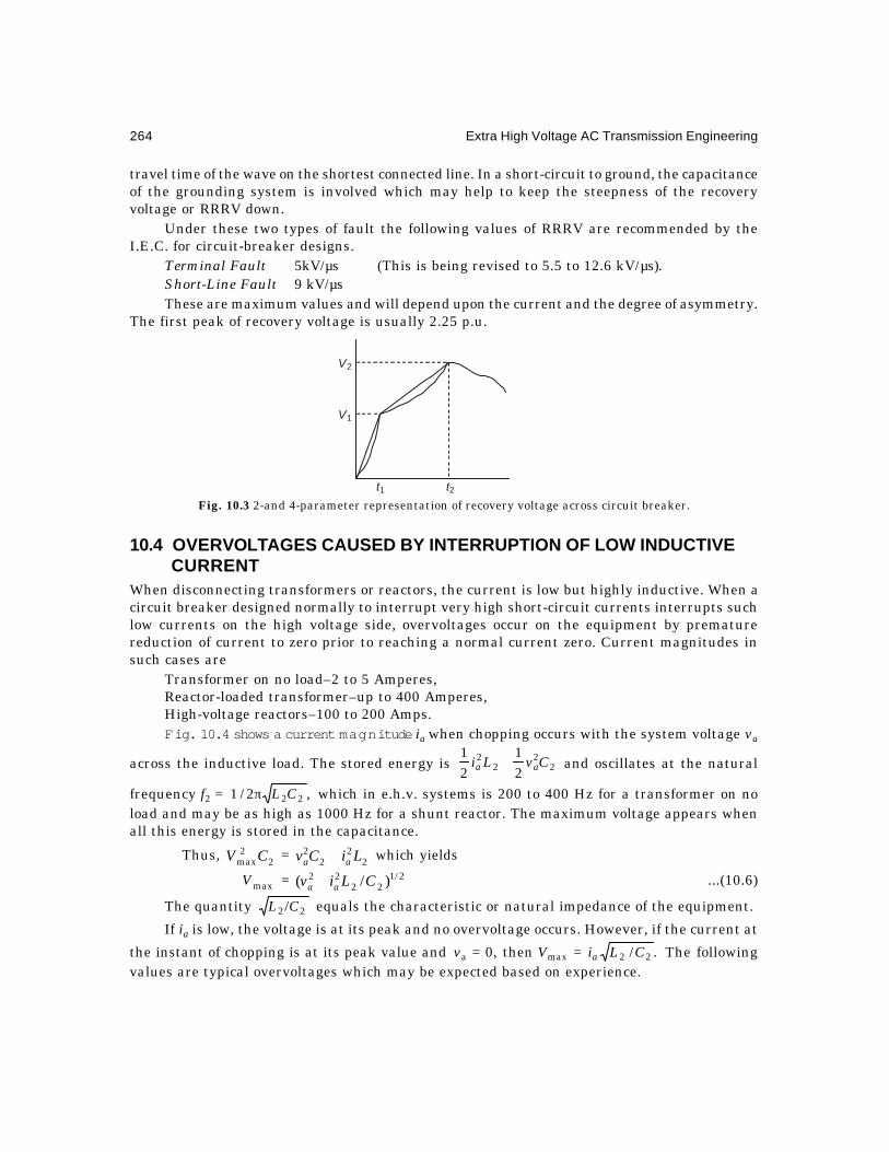
264 Extra High Voltage AC Transmission Engineering
travel time of the wave on the shortest connected line. In a short-circuit to ground, the capacitanceof the grounding system is involved which may help to keep the steepness of the recoveryvoltage or RRRV down.
Under these two types of fault the following values of RRRV are recommended by theI.E.C. for circuit-breaker designs.
Terminal Fault 5kV/µs (This is being revised to 5.5 to 12.6 kV/µs).Short-Line Fault 9 kV/µsThese are maximum values and will depend upon the current and the degree of asymmetry.
The first peak of recovery voltage is usually 2.25 p.u.
Fig. 10.3 2-and 4-parameter representation of recovery voltage across circuit breaker.
10.4 OVERVOLTAGES CAUSED BY INTERRUPTION OF LOW INDUCTIVECURRENT
When disconnecting transformers or reactors, the current is low but highly inductive. When acircuit breaker designed normally to interrupt very high short-circuit currents interrupts suchlow currents on the high voltage side, overvoltages occur on the equipment by prematurereduction of current to zero prior to reaching a normal current zero. Current magnitudes insuch cases are
Transformer on no load–2 to 5 Amperes,Reactor-loaded transformer–up to 400 Amperes,High-voltage reactors–100 to 200 Amps.Fig. 10.4 shows a current magnitude ia when chopping occurs with the system voltage va
across the inductive load. The stored energy is 22
22
21
21
CvLi aa + and oscillates at the natural
frequency f2 = ,2/1 22CLπ which in e.h.v. systems is 200 to 400 Hz for a transformer on noload and may be as high as 1000 Hz for a shunt reactor. The maximum voltage appears whenall this energy is stored in the capacitance.
Thus, 22
maxCV = 22
22 LiCv aa + which yields
maxV = 2/122
22 )/( CLiv aa + ...(10.6)
The quantity 22/CL equals the characteristic or natural impedance of the equipment.
If ia is low, the voltage is at its peak and no overvoltage occurs. However, if the current at
the instant of chopping is at its peak value and va = 0, then Vmax = ./ 22 CLia The followingvalues are typical overvoltages which may be expected based on experience.
V2
V1
t1 t2

Overvoltages in EHV Systems Caused by Switching Operations 265
220 kV – 2.5 p.u. 400 kV – 1.8 p.u. 750 kV– 1.2 p.u.This type of overvoltage can be reduced by surge arresters and series resistances used in
circuit breakers.
10.5 INTERRUPTION OF CAPACITIVE CURRENTSWhen transmission lines are dropped or de-energized or capacitor banks switched off,overvoltages are generated. Consider Fig. 10.4 where a line is represented by a lumpedcapacitance C2. Before interruption, V1 = V2.
Fig. 10.4 Conditions of voltage and current during 'current chopping' when interrupting low inductive currents.
After the current is interrupted C2 remains charged to 3/22 sVV = , which is the crestvalue of the source voltage at power frequency. However, the source voltage V1 changes polarity
and the breaker voltage is 3/2sb VV = (1 + K) where 1≈K , giving 3/22 sV . If the insulatingmedium in the breaker has not gained sufficient dielectric strength to withstand Vb, the arcmay restrike and connect the line to the source. A current flows which is 90° leading. When thecircuit is interrupted again at a current zero, the voltage is at its peak value and the line holdsa negative voltage. There may be repeated restrikes such as this and breaker failure mayoccur. See Fig. 10.5.
Therefore, restrike-free breakers are essential. Modern SF6 and airblast breakers meetthese requirements but in all cases proper maintenance is absolutely necessary. Lines equippedwith shunt reactors help to drain the trapped charge of the line and aid in proper interruption.Capacitor banks cause the same type of stresses on the circuit breaker.
V
Line CB i
L1
f1C1
LV1 f3
C2V2
f2L2
Va
ia
f3
Va
V2
f2
f1 V1

266 Extra High Voltage AC Transmission Engineering
Fig. 10.5 Voltages during re-striking of breaker when interrupting smallcapacitive currents (line dropping)
10.6 FERRO-RESONANCE OVERVOLTAGESPartial resonance conditions occur in power systems when unbalanced configuration occurs soas to place capacitances in series with inductances.
Fig. 10.6 Conditions leading to ferro-resonance during non-simultaneousoperation of circuit breaker poles.
When a transformer is connected to a long transmission line and both are switched together,such a condition might occur as shown in Fig. 10.6. Under normal operating conditions, theline capacitance to ground is energized by the phase voltage. However, suppose during aswitching operation, one pole opens or closes non-simultaneously with the others. The equivalentcircuit, Fig. 10.6(b), shows that the line capacitance is in series with the transformer inductancein the open phase. The condition when two poles are open may be seen in Fig. 10.6(b). The
i
V2
V1
V3
V1
Ec
LTEa
Sb
Sa Cr, l, c
CSb
Sc
LTN
LT
C
Sa
EaC
LTSb
EbC
LT
N
LTSc
C Ea
(a)
(b)

Overvoltages in EHV Systems Caused by Switching Operations 267
problem involves very difficult analysis and must take into account the distributed capacitanceof line and the non-linear magnetization curve of the transformer. This is a highly specializedtopic and will not be considered further. The problem is also very important in urban distributionwhere long cables are used underground and failures to both cable and transformer insulationshave resulted in great expense and inconvenience to consumers and power companies, especiallysince load-shedding and frequent switching has become common.
10.7 CALCULATION OF SWITCHING SURGES–SINGLE PHASEEQUIVALENTS
Switching operations in e.h.v. systems give rise to overvoltages due to the interaction betweenelectrostatic and electromagnetic energies trapped in the long lines which release in connectedequipment. Insulation designs are governed by these overvoltages and the remaining parts ofthis chapter will be devoted to the calculation of overvoltages and their reduction in practice.
We will commence the detailed discussion on formulating and solving equations controllingswitching surges with (a) lumped-parameter networks, then (b) distributed-parameter lines,and finally (c) a combination of both lumped-parameter elements connected to distributed-parameter lines. Some of these ideas have already been developed in Chapter 8 where thetheory was presented. A very good engineering idea of the magnitudes of switching surgesexperienced in system (c) can be obtained if systems (a) and (b) are first analyzed and theirresults interpreted.
10.7.1 Single-Frequency Lumped-Parameter CircuitConsider Figure 10.7 showing a series L-R-C circuit energized by a source e(t) by closing theswitch S. The capacitor has an initial trapped-charge voltage V0 with the polarity shown andthere is no initial current. The operational equation for the current using Laplace Transform is
sVsICsRLs /)()/1( 0+++ = E(s) ...(10.7)
giving I(s) =])[(
)(.20
20
wsLVsEs+α+
−...(10.8)
where α = 220 /1and2/ α−= LCwLR ...(10.9)
Fig. 10.7 (a) Lumped-parameter L-R-C circuit with initial voltage on capacitor.(b) Effect of increase of R on peak value of voltage across capacitor. (See Example 10.3)
e t( ) E S( )
S
Vc
L R
i
+V0
C
( )a
Vcp, P.U.3.0
2.0
1.0
10 40 100 632 103
R. ohms( )b
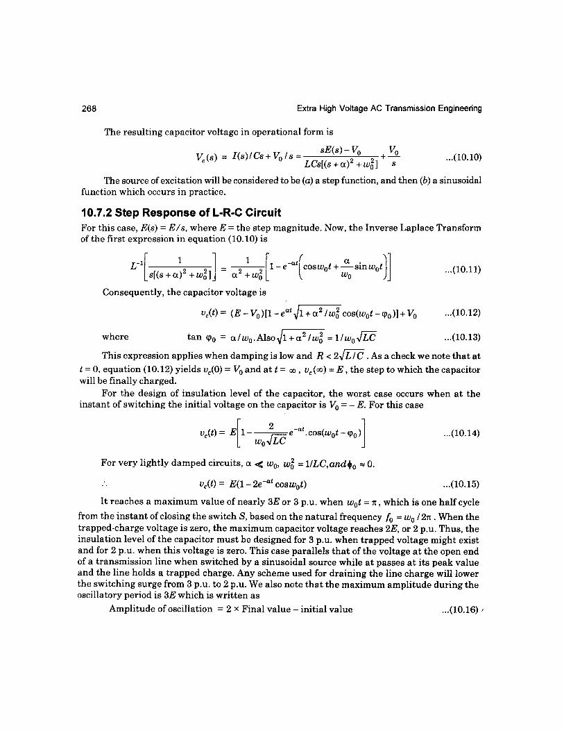
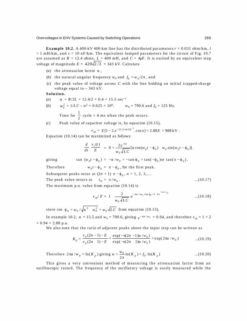
Overvoltages in EHV Systems Caused by Switching Operations 269
Example 10.2. A 400-kV 400-km line has the distributed parameters r = 0.031 ohm/km, l= 1 mH/km, and c = 10 nF/km. The equivalent lumped parameters for the circuit of Fig. 10.7are assumed as R = 12.4 ohms, L = 400 mH, and C = 4µF. It is excited by an equivalent stepvoltage of magnitude E = 3/2420 = 343 kV. Calculate
(a) the attenuation factor α ,
(b) the natural angular frequency w0 and π= 2/00 wf , and
(c) the peak value of voltage across C with the line holding an initial trapped-chargevoltage equal to – 343 kV.
Solution.(a) α = R/2L = 12.4/2 × 0.4 = 15.5 sec–1
(b) 20w = 1/LC – α2 = 0.625 × 10⁶. ∴ w0 = 790.6 and f0 = 125 Hz.
Time for 21
cycle = 4 ms when the peak occurs.
(c) Peak value of capacitor voltage is, by equation (10.15),
vcp = kV98888.2]cos..21[31045.15 ==π−
−××− EeE .Equation (10.14) can be maximized as follows:
E
tvdtd c )(
= )]sin()cos([2
0 000000
ϕ−+ϕ−α=α−
twwtwLCw
e t
.
giving tan )( 00 ϕ−tw = )tan(or)tan(tan/ 0000 ϕ−πϕ−=ϕ−=α− w .
Therefore 00 ϕ−tw = 0ϕ−π , for the first peak.
Subsequent peaks occur at (2n + 1) 0ϕ−π , n = 1, 2, 3,....The peak value occurs at tm = 0/wπ . ...(10.17)
The maximum p.u. value from equation (10.14) is
vcp/E =0/
00 21cos./
0
.2
1w
eweLCw
πα−+=ϕπα−+ ...(10.18)
since cos LCwww 020
200 / =+α=ϕ from equation (10.13).
In example 10.2, α = 15.5 and w0 = 790.6, giving 0/ we πα− = 0.94, and therefore vcp = 1 + 2
× 0.94 = 2.88 p.u.We also note that the ratio of adjacent peaks above the input step can be written as
Kp = )/2exp()/)12(exp(
)/)12(exp(
)12(
)12(0
0
0 wwnwn
Env
Env
p
p πα=α+π−α−π−
=−+
−−...(10.19)
Therefore )ln(.)ln(2
giving)ln(/2 00
0 ppp KfKwKw =π
=α=πα ...(10.20)
This gives a very convenient method of measuring the attenuation factor from anoscilloscopic record. The frequency of the oscillatory voltage is easily measured while the
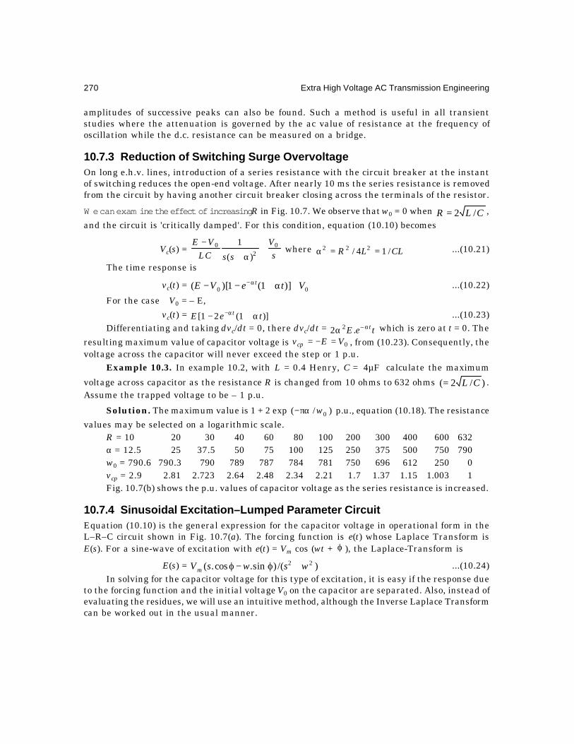
270 Extra High Voltage AC Transmission Engineering
amplitudes of successive peaks can also be found. Such a method is useful in all transientstudies where the attenuation is governed by the ac value of resistance at the frequency ofoscillation while the d.c. resistance can be measured on a bridge.
10.7.3 Reduction of Switching Surge OvervoltageOn long e.h.v. lines, introduction of a series resistance with the circuit breaker at the instantof switching reduces the open-end voltage. After nearly 10 ms the series resistance is removedfrom the circuit by having another circuit breaker closing across the terminals of the resistor.
W e can exam ine the effect of increasing R in Fig. 10.7. We observe that w0 = 0 when CLR /2= ,
and the circuit is 'critically damped'. For this condition, equation (10.10) becomes
Vc(s) =s
V
ssLCVE 0
20
)(
1+
α+
− where CLLR /14/ 222 ==α ...(10.21)
The time response is
vc(t) = 00 )]1(1)[( VteVE t +α+−− α− ...(10.22)
For the case V0 = – E,
vc(t) = )]1(21[ teE t α+− α− ...(10.23)Differentiating and taking dvc/dt = 0, there dvc/dt = teE tαα –2 .2 which is zero at t = 0. The
resulting maximum value of capacitor voltage is 0VEvcp =−= , from (10.23). Consequently, thevoltage across the capacitor will never exceed the step or 1 p.u.
Example 10.3. In example 10.2, with L = 0.4 Henry, C = F4µ calculate the maximum
voltage across capacitor as the resistance R is changed from 10 ohms to 632 ohms )/2( CL= .Assume the trapped voltage to be – 1 p.u.
Solution. The maximum value is 1 + 2 exp )/( 0wπα− p.u., equation (10.18). The resistance
values may be selected on a logarithmic scale.R = 10 20 30 40 60 80 100 200 300 400 600 632α = 12.5 25 37.5 50 75 100 125 250 375 500 750 790w0 = 790.6 790.3 790 789 787 784 781 750 696 612 250 0vcp = 2.9 2.81 2.723 2.64 2.48 2.34 2.21 1.7 1.37 1.15 1.003 1Fig. 10.7(b) shows the p.u. values of capacitor voltage as the series resistance is increased.
10.7.4 Sinusoidal Excitation–Lumped Parameter CircuitEquation (10.10) is the general expression for the capacitor voltage in operational form in theL–R–C circuit shown in Fig. 10.7(a). The forcing function is e(t) whose Laplace Transform isE(s). For a sine-wave of excitation with e(t) = Vm cos (wt + ϕ ), the Laplace-Transform is
E(s) = )/()sin.cos.( 22 wswsVm +ϕ−ϕ ...(10.24)In solving for the capacitor voltage for this type of excitation, it is easy if the response due
to the forcing function and the initial voltage V0 on the capacitor are separated. Also, instead ofevaluating the residues, we will use an intuitive method, although the Inverse Laplace Transformcan be worked out in the usual manner.

Overvoltages in EHV Systems Caused by Switching Operations 271
Response due to Initial Trapped Voltage V0
For this voltage, the operational expression for the capacitor voltage in equation (10.10) is
V0(s) =]).[(
1.
20
200
wssLCV
sV
+α+− ...(10.25)
The inverse transform is, using equation (10.11),
v0(t) = )]cos(./1.11[ 0020
20 ϕ−α+−− α− twweV t
= )cos(. 000
0 ϕ−α− tweLCw
V t...(10.26)
where the values of α , w0 and 0ϕ are taken from equations (10.9) and (10.13). The above
solution is valid for CLR /2< .
For the critically-damped case, R = 0,/2 0 =wCL , it becomes
v0(t) = )]1(1)/1(1[ 20 teLCV t α+−α− α−
= )]2/1(1)/4(1[ 20 LRteCRLV t +−− α− ...(10.27)
The quantity CL / can be called the natural impedance Z0 of the L-R-C circuit, giving
4L/R2C = 220 /4 RZ . Thus, the magnitude of the second quantity in (10.27) depends on the ratio
of characteristic impedance to the actual resistance included in the network. Also, CRL 2/4 =1 for the critically damped case.
Response due to Forcing Function e(t) = Vm cos (wt + ϕϕ)The transient resulting from sudden energization of the circuit will consist of two parts whichare (1) the steady state term or particular integral surviving when all transients have vanished,and (2) the exponentially decaying transient term or the complimentary function.
(1) Steady-State Term
Using phasor algebra, the circuit current phasor leads the applied voltage by the angle ψand the magnitude is Vm/Z. Thus, its value is
Iss = )cos( ψ+ϕ+wtZ
Vm ...(10.28)
−=ψ
−+=
]/)/1tan[(arcand
)/1(where 22
RwLwC
wLwCRZ...(10.29)
The capacitor voltage in the steady state lags 90° behind the current and has the value
Vcs = )sin(901 ψ+ϕ+=°−∠ wt
wCZVI
wCm
ss ...(10.30)
(2) Complimentary Function or Transient Term
The transient term will be of the same form as equation (10.11) and is written as
Vcc =tetwKtwK α−+ )sincos( 0201 , ...(10.31)

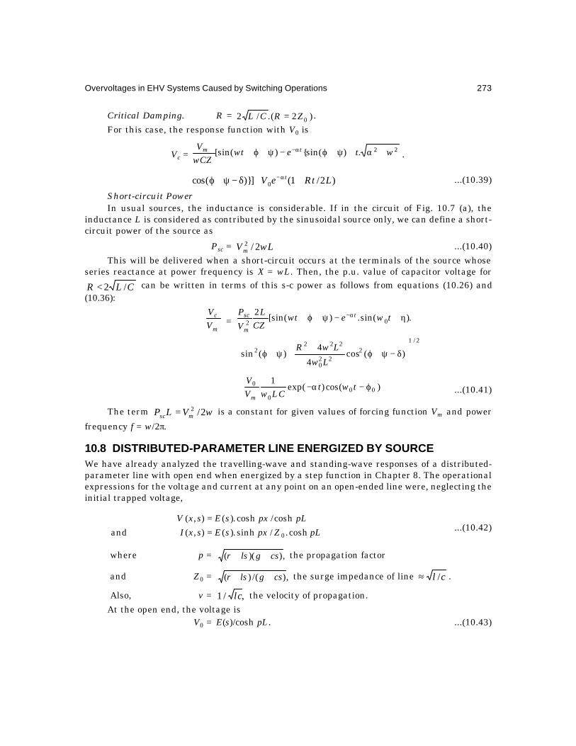
Overvoltages in EHV Systems Caused by Switching Operations 273
Critical Damping. R = )2.(/2 0ZRCL = .For this case, the response function with V0 is
Vc =22.)sin()[sin( wtewt
wCZV tm +α+ψ+ϕ−ψ+ϕ+ α−
.
)2/1()]cos( 0 LRteV t ++δ−ψ+ϕ α− ...(10.39)
Short-circuit PowerIn usual sources, the inductance is considerable. If in the circuit of Fig. 10.7 (a), the
inductance L is considered as contributed by the sinusoidal source only, we can define a short-circuit power of the source as
Psc = wLVm 2/2 ...(10.40)
This will be delivered when a short-circuit occurs at the terminals of the source whoseseries reactance at power frequency is X = wL. Then, the p.u. value of capacitor voltage for
CLR /2< can be written in terms of this s-c power as follows from equations (10.26) and(10.36):
m
c
VV
= ).sin(.)[sin(2
02η+−ψ+ϕ+ α− twewt
CZL
VP t
m
sc
δ−ψ+ϕ
++ψ+ϕ
2/1
222
0
2222 )(cos
4
4)(sin
Lw
LwR
)cos()exp(1
000
0 ϕ−α−+ twtLCwV
V
m...(10.41)
The term wVLP msc 2/2= is a constant for given values of forcing function Vm and power
frequency f = w/2π.
10.8 DISTRIBUTED-PARAMETER LINE ENERGIZED BY SOURCEWe have already analyzed the travelling-wave and standing-wave responses of a distributed-parameter line with open end when energized by a step function in Chapter 8. The operationalexpressions for the voltage and current at any point on an open-ended line were, neglecting theinitial trapped voltage,
==
pLZpxsEsxIpLpxsEsxV
cosh./sinh).(),(and
cosh/cosh).(),(
0...(10.42)
where p = ,))(( csglsr ++ the propagation factor
and Z0 = ,)/()( csglsr ++ the surge impedance of line cl /≈ .
Also, v = ,/1 lc the velocity of propagation.
At the open end, the voltage isV0 = E(s)/cosh pL. ...(10.43)

274 Extra High Voltage AC Transmission Engineering
Step Response. Denoting A0 = e–aL where 02/2/ Zrlvra == , the step response was obtainedas shown in Fig. 8.4 and the Bewley Lattice Diagram, Figure 8.5. The general expression forthe voltage at time t = NT, where T = time taken for travel of surge over one line length (T =
L/v) was ,2 )2(200 TNNT VAAV −−= N odd. The maximum voltage is 2A0 at the open end when
trapped charge is neglected. With a trapped voltage of 1 p.u., the open-end voltage reaches amaximum of (2A0 + 1) p.u. In usual transmission lines, the trapped voltage is 0.8 p.u. on areclosing operation. We may note here that the value of first peak is very nearly the same aswas obtained from the lumped-parameter network.
The attenuation factor must be properly calculated by considering the resistance of notonly the conductor but also the ground return which exceeds the conductor resistance by afactor of as much as 10. The following example shows the effect of ground-return inductance onthe velocity of propagation and the resistance on the attenuation.
Example 10.4. The 400-km 400-kV line considered in example 10.2 has the followingdetails:
Conductor resistance rc = 0.031 ohm/kmGround return resistance rg = 0.329 ohm/km at 125 HzSeries inductance of line ls = 1 mH/kmGround-return inductance lg = 0.5 mH/kmShunt capacitance c = 11.1 nF/kmCalculate(a) velocity of propagation v and travel time T;(b) surge impedance;(c) attenuation factor A0;(d) maximum p.u. value of open-end voltage without trapped voltage.Compare all these quantities by neglecting ground and considering the ground-return
parameters.Solution.
Neglecting rg and lg Considering rg and lgTotal resistance r 0.031 ohm/km 0.36 ohm/kmTotal inductance l 1 mH/km 1.5 mH/kmCapacitance c 11.1 nF/km 11.1 nF/km
Velocity v, km/sec 3 × 10⁵ 1.115.1/106 ×= 2.45 × 105 = 82% light velocity
Time for 1 travel, T, ms 1.33 1.633
Surge impedance 300 367101.11/5.1 3 =×Z0, ohmsAttenuation factor, A0 98.0800/4.12 =−e 822.0734/144 =−eMaximum open-end 1.96 p.u. 1.644 p.u.voltage, 2A0
We note that the effect of ground-return resistance and inductance on the switching surgeresponse (step response) is to
(a) decrease the velocity of propagation of the surge,(b) increase the time of travel,
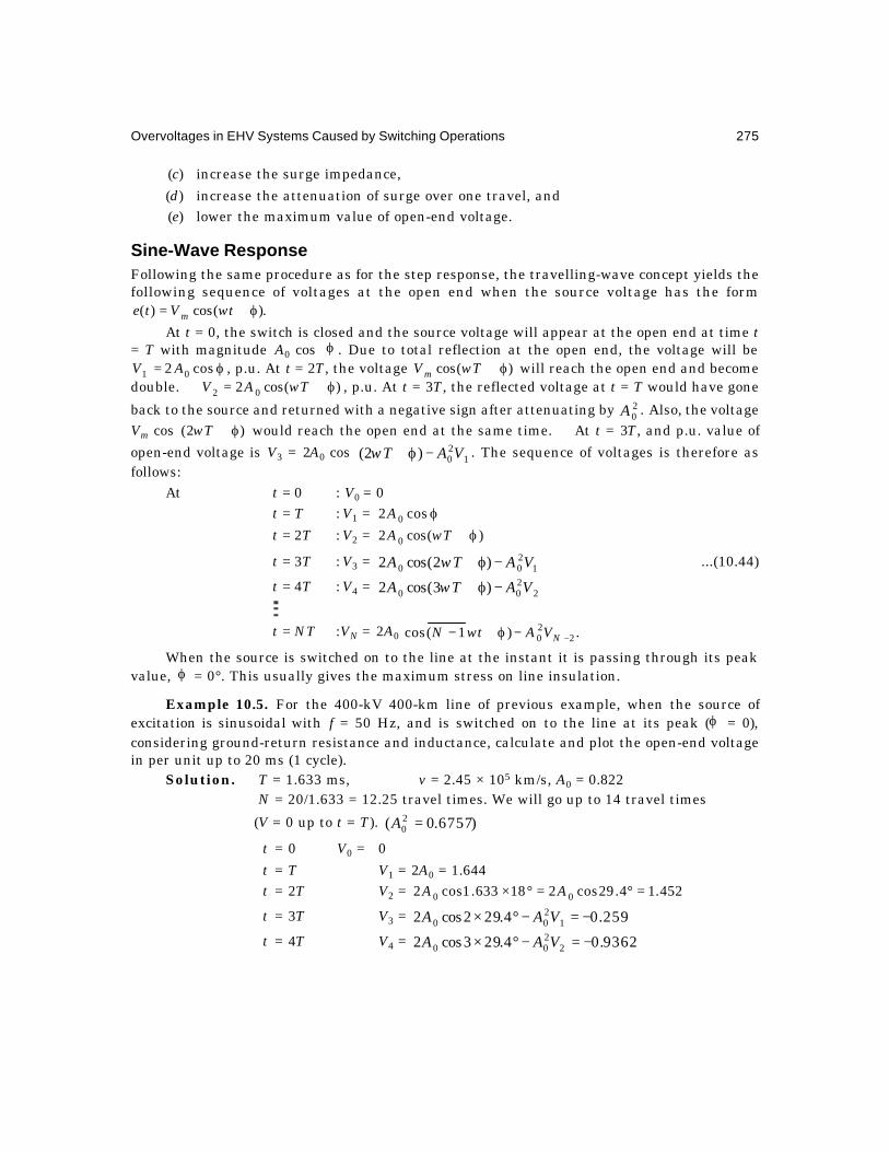
Overvoltages in EHV Systems Caused by Switching Operations 275
(c) increase the surge impedance,
(d) increase the attenuation of surge over one travel, and(e) lower the maximum value of open-end voltage.
Sine-Wave ResponseFollowing the same procedure as for the step response, the travelling-wave concept yields thefollowing sequence of voltages at the open end when the source voltage has the form
).cos()( ϕ+= wtVte m
At t = 0, the switch is closed and the source voltage will appear at the open end at time t= T with magnitude A0 cos ϕ . Due to total reflection at the open end, the voltage will be
ϕ= cos2 01 AV , p.u. At t = 2T, the voltage )cos( ϕ+wTVm will reach the open end and becomedouble. ∴ )cos(2 02 ϕ+= wTAV , p.u. At t = 3T, the reflected voltage at t = T would have gone
back to the source and returned with a negative sign after attenuating by 20A . Also, the voltage
Vm cos )2( ϕ+wT would reach the open end at the same time. ∴ At t = 3T, and p.u. value of
open-end voltage is V3 = 2A0 cos 120)2( VAwT −ϕ+ . The sequence of voltages is therefore as
follows:At t = 0 : V0 = 0
t = T : V1 = ϕcos2 0At = 2T : V2 = )cos(2 0 ϕ+wTA
t = 3T : V3 = 1200 )2cos(2 VAwTA −ϕ+ ...(10.44)
t = 4T : V4 = 2200 )3cos(2 VAwTA −ϕ+
t = NT :VN = 2A0 .)1(cos 220 −−ϕ+− NVAwtN
When the source is switched on to the line at the instant it is passing through its peakvalue, ϕ = 0°. This usually gives the maximum stress on line insulation.
Example 10.5. For the 400-kV 400-km line of previous example, when the source ofexcitation is sinusoidal with f = 50 Hz, and is switched on to the line at its peak (ϕ = 0),considering ground-return resistance and inductance, calculate and plot the open-end voltagein per unit up to 20 ms (1 cycle).
Solution. T = 1.633 ms, v = 2.45 × 10⁵ km/s, A0 = 0.822∴ N = 20/1.633 = 12.25 travel times. We will go up to 14 travel times
(V = 0 up to t = T). )6757.0( 20 =A
t = 0 V0 = 0
t = T V1 = 2A0 = 1.644t = 2T V2 = 452.14.29cos218633.1cos2 00 =°=°× AA
t = 3T V3 = 259.04.292cos2 1200 −=−°× VAA
t = 4T V4 = 9362.04.293cos2 2200 −=−°× VAA

276 Extra High Voltage AC Transmission Engineering
Continuing in this manner, we obtainV5 = – 0.587, V6 = – 0.746, V7 = – 1.244, V8 = – 0.976, V9 = – 0.098,
V10 = 0.5037, V11 = 0.735, V12 = 0.98, V13 = 1.134,
and V14 = 86.04.2913cos2 12200 =−°× VAA
The oscillations have nearly vanished and the open-end voltage follows the source voltageas shown in Fig. 10.8.
Fig. 10.8 Open-end voltage on a line excited by a sinusoidal source.
10.9 GENERALIZED EQUATIONS FOR SINGLE-PHASE REPRESENTATIONA more general case with series and shunt impedance lumped elements connected to distributed-parameter line was considered in chapter 8, section 8.10. It was shown that the voltage at theentrance to the line was, with a little re-writing of equation (8.122),
Ve =
pLZZ
ZZZZ
ZZ
pLZZ
ZZ
pLZZpLsE
s
tsh
s
tt
s
sh
s
t
sinhcosh1
sinh)/(cosh).(
0
00
0
+++
++
+...(10.45)
Having found Ve, all other voltages and curents can be obtained. In particular, the voltageat the far end or at the termination is
V0 =
+++
++ pL
ZZ
ZZZZ
ZZ
pLZZ
ZZ
sE s
tsh
s
tt
s
sh
s sinhcosh1)(0
00 ...(10.46)
These form the generalized equations for a single-phase representation of the system.These equations also yield the more complicated set of performance equations of a 3-phasesystem if all quantities are suitably replaced by matrices. This will be taken up in the nextsection. The matrices can be diagonalized to yield three mutually-decoupled single-phase systemsor modes of propagation for the surge. Obtaining the inverse transform to yield the correspondingtime variation in closed form is not easy for a general case and must be attempted through theFourier Transform or other methods suitable for the Digital Computer.
Particular Cases of the General EquationsEquations (10.45) and (10.46) for the entrance and termination voltages can be used for
particular cases which occur in practice. Some typical cases are shown in the tabular form. 7cases are considered which are shown in Fig. 10.9.
2.0
1.0
0
– 1.0
– 2.0
1 2
3
4 5 6 7 8
9
10 11 12 13 14
V0
t/T

Overvoltages in EHV Systems Caused by Switching Operations 277
S.No. System Impedances Open-end Voltage V0 Entrance Voltage Ve
Configuration
1. Figure 10.9 (a) ∞=
∞==
t
shs
ZZZ ,0 E(s)/cosh pL E(s)
2. Figure 10.9(b)
sht
shs
ZZZZ
== ,,0
pLZZpL
sE
sh
sinhcosh
)(
0+E(s)
3. Figure (10.9)(c)∞=
=
sh
ts
ZZZ ,0
pLZZpL
sE
t
sinhcosh
)(
0+E(s)
4. Figure 10.9(d)∞=
∞=
t
shs
ZZZ ,
pLZZpL
sE
s sinhcosh
)(
0
+pLV cosh.0
5. Figure 10.9(e)∞=t
shs
ZZZ ,
pLZZ
pLZZ
sE
s
sh
s sinhcosh1
)(
0+
+
pLV cosh.0
6. Figure 10.9( f )
sht
shs
ZZ
ZZ
=,,
pLZ
ZZZZ
ZZ
pLZZ
sE
sh
ss
sh
sh
s
sinh
cosh2
1
)(
20
0
0
++
+
+
+
pLZZ
pLV
sh
sinh
cosh
0
0
7. Figure 10.9(g)
t
shs
ZZZ ,, Equation 10.46 Equation 10.45
Line
E
E Zsh
Ve V0
Zt
Ve V0( )a
( )b
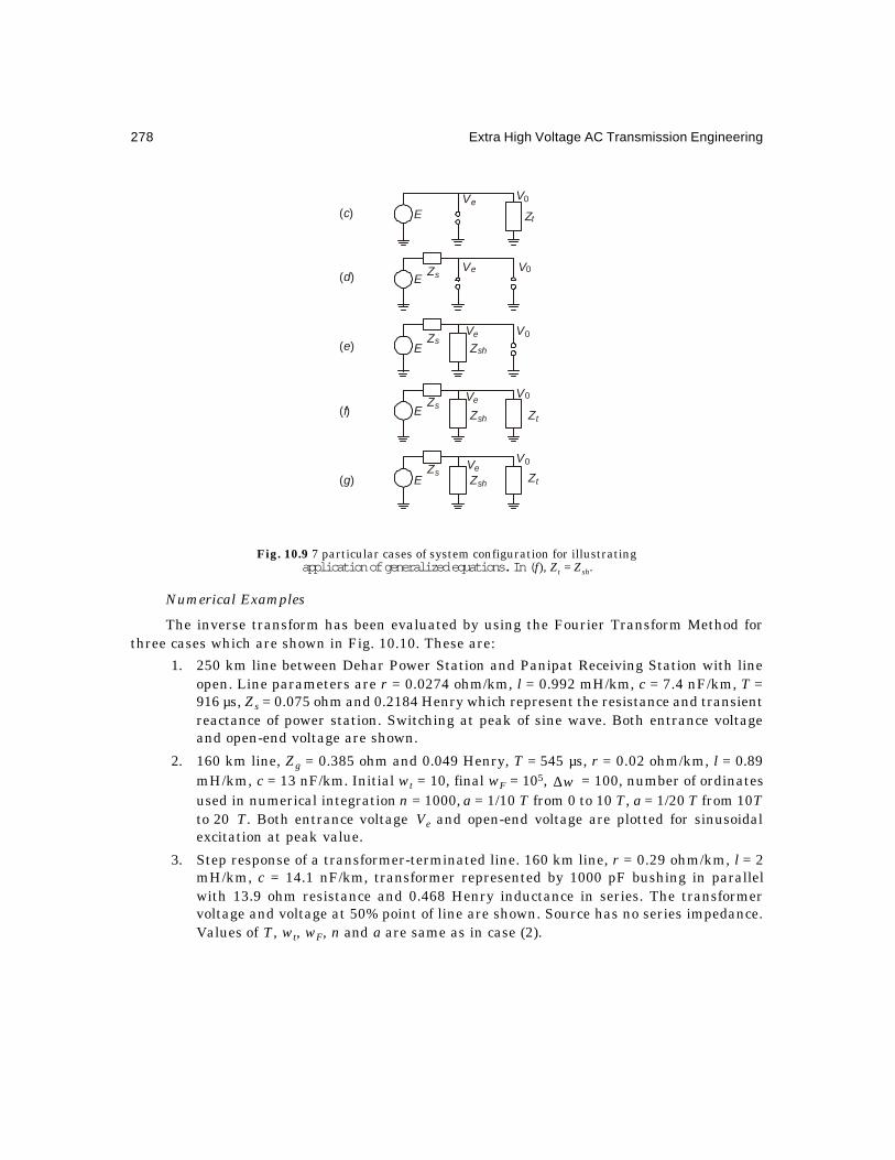
278 Extra High Voltage AC Transmission Engineering
Fig. 10.9 7 particular cases of system configuration for illustratingapplication of generalized equations. In (f), Zt = Zsh.
Numerical Examples
The inverse transform has been evaluated by using the Fourier Transform Method forthree cases which are shown in Fig. 10.10. These are:
1. 250 km line between Dehar Power Station and Panipat Receiving Station with lineopen. Line parameters are r = 0.0274 ohm/km, l = 0.992 mH/km, c = 7.4 nF/km, T =916 µs, Zs = 0.075 ohm and 0.2184 Henry which represent the resistance and transientreactance of power station. Switching at peak of sine wave. Both entrance voltageand open-end voltage are shown.
2. 160 km line, Zg = 0.385 ohm and 0.049 Henry, T = 545 µs, r = 0.02 ohm/km, l = 0.89mH/km, c = 13 nF/km. Initial wt = 10, final wF = 105, w∆ = 100, number of ordinatesused in numerical integration n = 1000, a = 1/10 T from 0 to 10 T, a = 1/20 T from 10Tto 20 T. Both entrance voltage Ve and open-end voltage are plotted for sinusoidalexcitation at peak value.
3. Step response of a transformer-terminated line. 160 km line, r = 0.29 ohm/km, l = 2mH/km, c = 14.1 nF/km, transformer represented by 1000 pF bushing in parallelwith 13.9 ohm resistance and 0.468 Henry inductance in series. The transformervoltage and voltage at 50% point of line are shown. Source has no series impedance.Values of T, wt, wF, n and a are same as in case (2).
E
E
E
E
E
Ve
Ve
Ve
Zsh
Zsh
Zsh
Zt
Zt
Ve
Ve
V0
V0
V0
Zs
Zs
Zs
Zs
V0
V0
Zt( )c
( )d
( )e
( )f
( )g

Overvoltages in EHV Systems Caused by Switching Operations 279
Fig. 10.10 Overvoltages during switching operations on systems calculated by Fourier Transforms.(a) 250 km line energized at peak of sine wave at generating station with series impedance. (b) 160 km lineenergized at peak of sine wave, with source having small inductance (sub-transient). (c) Step response of areceiving-station transformer termination. No source series impedance.
Ve V0Ve
V0
V
2.0
1.5
1.0
0.5
0 2T 4T 8T 12T 14T 16T
Tn = 545 s = 1000
µ.0488
160 km
Ve V0
V
.075250 km = 916 sT µ
.2184 H
Dehar
T 2T 3T 5T 6T 7T
1.0
( )a
( )b
( )c
0.5Ve
V0VDehar
Panipat
1.5
1.0
0.5
0T 2T 4T 6T 8T 12T 16T14T
V5V0STEP
S 160 km 1 nF
.468 H13.9 Ω
V5 V0

280 Extra High Voltage AC Transmission Engineering
10.10 GENERALIZED EQUATIONS FOR THREE-PHASE SYSTEMSThe generalized equations for switching-surge calculation on 3-phase systems is an extensionof the single-phase case of the previous section. Since the equations are quite lengthy, a step bystep procedure is given below. We will restrict the development to a fully transposed line.
Resistance of LineWith ground-return considered, the total resistance consists of conductor resistance rc
and ground-return resistance rg. The resulting matrix of resistance will be
[r] = ][][ DrUr gc + ...(10.47)
where [U] =
=
1,1,1
1,1,1
1,1,1
][and
1,0,0
0,1,0
0,01
D ...(10.48)
Inductance of Line: In a similar manner
[l] = ])[(])[( DllUll gmms ++− ...(10.49)where ls = self inductance, lm = mutual inductance between phases, and lg = ground-return
inductance per unit length.Capacitance of Line
[c] = ][])[( DcUcc mms +− ...(10.50)
Shunt Impedance at line entrance[Zsh] = Zsh[U] ...(10.51)
Series Impedance of source[Zs] = Zs[U] ...(10.52)
Terminating ImpedanceFor balanced condition
[Zt] = Zt[U] ...(10.53)For general unbalanced condition,
[Zt] =
3
2
1
,
t
t
t
ZZ
Z
...(10.54)
Source Voltage
[e(t)] =
ϕ+ϕ+ϕ+
)cos(
)cos(
)cos(
3
2
1
wtwtwt
Vm ...(10.55)
For synchronous closing.
2ϕ = °+ϕ=ϕ°−ϕ 120,120 131
The angles 321 ,, ϕϕϕ denote the points on the wave at which switching takes place fromthe positive peaks of the respective phase voltages.

Overvoltages in EHV Systems Caused by Switching Operations 281
Voltage EquationsCommencing with the output end, we have the following sequence of equations, as shown
from Fig. 10.11.[V0] = [Zt] [I0], [V0] = [F] [Ve] ...(10.56)
where [F] is a function which is to be determined from the differential equations. For asingle-phase representation, F is given by the ratio of equations (10.46) and (10.45), which is
]sinh)/([cosh 0 pLZZpL t+ . ]][[][ ee VGI = where [G] is another function still to be evaluated.
Refer to Chapter 8 for the single-phase case. A similar value in matrix form can be derived.
Fig. 10.11 General representation of a system.
[Is] = [Ie] + [Zsh]–1 [Ve] ...(10.57)[E] = Laplace transform of source voltages
= ][][]][[][]][[][ 1eshesesse VZIZVIZV −++=+
= ]][][]][[][[ 1eshs VZGZU −++ ...(10.58)
∴ The entrance voltage is
[Ve ] = [[U ] + [Zs ] [G] + [Zsh ]–1]–1 [E ] ...(10.59)
Having obtained the entrance voltage in terms of the source voltage [E], the output voltage[V0] and the currents can be obtained in operational form. The time-domain solutions have tobe evaluated by the Inverse Transform.
10.10.1 Resolution into Component Modes of PropagationIn equations (10.47) to (10.50), the line parameters involve the special matrix [D]. If this isdiagonalized, then the voltages and currents can all be resolved into components which willshow no mutual interaction. They are resolved into three 'modes of propagation.' At any desiredtime, they can be recombined to yield the phase quantities. This can be carried out by theDigital Computer after every calculation of the inverse transform.
It has been shown in Chapter 3 that the modified Clarke Transformation matrix willdiagonalize [D]. The matrices are
[T] =
−−=
−− −
12,1
30,3
2,2,2
6
1][and
1,3,2
2,0,2
1,3,2
6
1 1T ...(10.60)
[ ]Zs
[ ( )][Z ]E s sh
[ ]Is [ ]Ie [ ]I0
[ ]Zt [ ]V0[ ]Ve
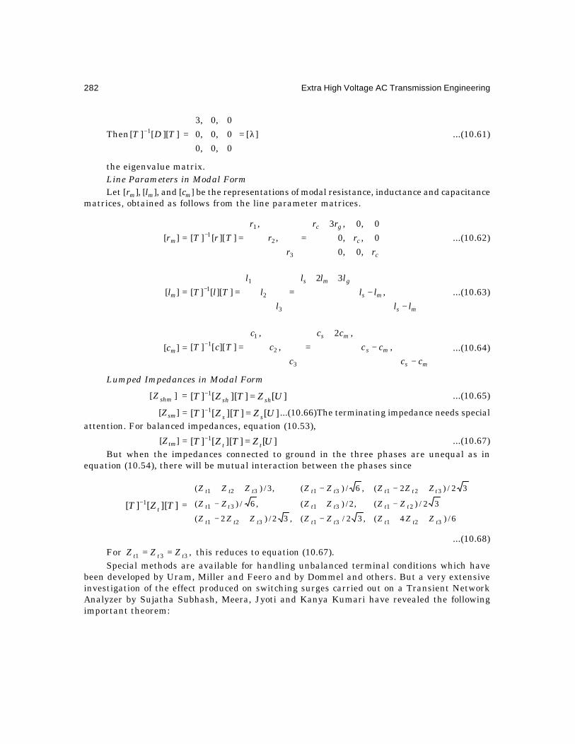
282 Extra High Voltage AC Transmission Engineering
Then ]][[][ 1 TDT − = ][
0,0,0
0,0,0
0,0,3
λ=
...(10.61)
the eigenvalue matrix.Line Parameters in Modal FormLet [rm], [lm], and [cm] be the representations of modal resistance, inductance and capacitance
matrices, obtained as follows from the line parameter matrices.
[rm] =
+=
=−
c
c
gc
rr
rr
rr
rTrT
,0,0
0,,0
0,0,3
,
,
]][[][
3
2
11 ...(10.62)
[lm] =
−−
++=
=−
ms
ms
gms
llll
lll
ll
lTlT ,
32
]][[][
3
2
11 ...(10.63)
[cm] =
−−
+=
=−
ms
ms
ms
cccc
cc
cc
cTcT ,
,2
,
,
]][[][
3
2
11 ...(10.64)
Lumped Impedances in Modal Form
][ shmZ = ][]][[][ 1 UZTZT shsh =− ...(10.65)
[Zsm] = ][]][[][ 1 UZTZT ss =− ...(10.66)The terminating impedance needs specialattention. For balanced impedances, equation (10.53),
[Ztm] = ][]][[][ 1 UZTZT tt =− ...(10.67)But when the impedances connected to ground in the three phases are unequal as in
equation (10.54), there will be mutual interaction between the phases since
]][[][ 1 TZT t− =
++−+−
−+−
+−−++
6/)4(,32/(,32/)2(
32/)(,2/)(,6/)(
32/)2(,6/)(,3/)(
32131321
213131
32131321
tttttttt
tttttt
tttttttt
ZZZZZZZZ
ZZZZZZ
ZZZZZZZZ
...(10.68)For ,331 ttt ZZZ == this reduces to equation (10.67).Special methods are available for handling unbalanced terminal conditions which have
been developed by Uram, Miller and Feero and by Dommel and others. But a very extensiveinvestigation of the effect produced on switching surges carried out on a Transient NetworkAnalyzer by Sujatha Subhash, Meera, Jyoti and Kanya Kumari have revealed the followingimportant theorem:

Overvoltages in EHV Systems Caused by Switching Operations 283
'When unbalanced terminal conditions exist, the system response to switching is nearlythe same as if the system consists of three balanced systems, each one having terminatingimpedances equal to those connected in the individual phases.' Using this property, the systemcan be analyzed three times by using balanced load of Zt1 in all phases and calculating theswitching-surge response in phase 1. Then replace a balanced load of Zt2 and determine theresponse of phase 2. Finally, replace a balanced load Zt3 in the system and the resulting responseof phase 3 will be the same as when the unbalanced load is used. We might also remark thatsince switching-surge calculations under unbalanced loads or when considering resistances inlines is very complicated and consumes a very long computer time, shorter methods, givingresults acceptable for engineering designs must be continuously devised. Hedman has foundthat the line resistance can be omitted in solving the travelling-wave equations but can beincluded as a lumped series resistance with the load. Similarly, the problems of frequency-dependence of ground-return parameters have also caused grave concern and form very advancedtopics which cannot be discussed in this introductory chapter to calculation of switching surges.The reader is referred to the extensive work listed in the bibliography.
Voltages and Currents in Modal Form: Differential Equations:Source Voltage
])][([][ 1 TteT − =
ϕ++ϕ+−ϕ+ϕ+−ϕ+
ϕ++ϕ++ϕ+
)cos()cos(2)cos(
)cos()cos(3
)cos()cos()cos(2
631
31
321
wtwtwtwtwt
wtwtwtVm
...(10.69)
The operational forms of these voltages can be evaluated suitably by using )][cos( ϕ+wtL
= )/()sin.cos.( 22 wsws +ϕ−ϕ .
The governing differential equations and their solutions for each of the three independentmodes can now be derived. The basic differential equation for the phase quantities are
dxVd x ][
= ][][][
and],[][][ xx
x VscdxIdIslr =+ ...(10.70)
These are resolved into modal form thus:
][][ 1xV
dxdT −
= ][][][
3
2
11
m
m
m
m
x Vdxd
VVV
dxd
VTdxd
=
=−
...(10.71)
But [T]–1 [r] + [l]s [T] [T]–1 [Ix] = [rm] + [lm]s [Im] ...(10.72)
∴ ][ mVdxd
= [rm] + [lm]s [Im] ...(10.73)
Similarly, ][ mIdxd
= [cm] s[Vm] (10.74)
These constitute 6 independent equations which are as follows by using equations (10.62)to (10.64):
−+=
−+=
++++=
mmscm
mmscm
mgmsgcm
IsllrdxdV
IsllrdxdV
IslllrrdxdV
33
22
11
)/
)(/
)32()3(/
...(10.75)

284 Extra High Voltage AC Transmission Engineering
−=−=
+=
mmsm
mmsm
mmsm
VsccdxdIVsccdxdI
VsccdxdI
33
22
11
.)(/
.)(/
.)2(/
...(10.75)
We observe that these are equivalent to the following 3 sets of equations, one for eachmode, as if each pertains to a single-phase quantity but in modal form,
d (Vkm)/dx = zkm.Ikm, and d(Ikm)/dx = ykm Vkm ...(10.76)where k = 1, 2, 3. Omitting the subscripts, for any one of the modes, the differential
equations are of the formdV/dx = zI, and dI/dx = yV ...(10.77)
−=
+=
−
−
)(1
and
aresolutionsTheir
0
pxpx
pxpx
BeAeZ
I
BeAeV
...(10.78)
We have encountered these before in Chapter 8. In these equations, the propagationfactor p and surge impedance Z0 belong to the mode under consideration, and their values areas follows:
Mode 1:
p1 = ])2()2()3[( sccslllrr msgmsgc +++++
+=
+=
scslrZ
scslr
11101
111
/)(
)(...(10.79)
Mode 2:
p2 = scslrZscslr 22202222 /)(,)( +=+ ...(10.80)
Mode 3:p3 = p2 and Z03 = Z02 ...(10.81)
The values of r1, r2, l1, l2, c1, c2 are given in equations (10.62) to (10.64). Equations (10.78)can be applied for each mode in turn which will yield expressions for the required voltages orcurrents in the system when the entrance voltage Ve to the line is found in terms of the sourcevoltage as shown in equations (10.45) and (10.46) for a single phase case.
After having calculated the inverse transform at every instant of time by a suitable methodon the Digital Computer, the modal voltages and currents can be re-converted to phase quantitiesby the inverse transformation to equations (10.71) to (10.74):
[Vph] = [T] [Vm] and [Iph] = [T] [Im] ...(10.82)For example,
3
2
1
ph
ph
ph
VVV
=
−−
m
m
m
VVV
3
2
1
1,3,2
2,0,2
1,3,2
6
1
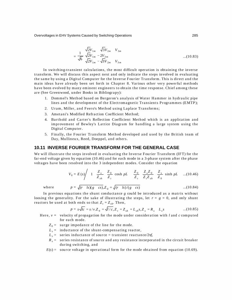
Overvoltages in EHV Systems Caused by Switching Operations 285
=
+−−
++
mmm
mm
mmm
VVVVV
VVV
321
31
321
32
22
32
6
1...(10.83)
In switching-transient calculations, the most difficult operation is obtaining the inversetransform. We will discuss this aspect next and only indicate the steps involved in evaluatingthe same by using a Digital Computer for the Inverse Fourier Transform. This is direct and themain ideas have already been set forth in Chapter 8. Various other very powerful methodshave been evolved by many eminent engineers to obtain the time response. Chief among theseare (See Greenwood, under Books in Bibliograpy):
1. Dommel's Method based on Bergeron's analysis of Water Hammer in hydraulic pipelines and the development of the Electromagnetic Transients Programmes (EMTP);
2. Uram, Miller, and Feero's Method using Laplace Transforms;
3. Ametani's Modified Refraction Coefficient Method;4. Barthold and Carter's Reflection Coefficient Method which is an application and
improvement of Bewley's Lattice Diagram for handling a large system using theDigital Computer.
5. Finally, the Fourier Transform Method developed and used by the British team ofDay, Mullineux, Reed, Doeppel, and others.
10.11 INVERSE FOURIER TRANSFORM FOR THE GENERAL CASEWe will illustrate the steps involved in evaluating the Inverse Fourier Transform (IFT) for thefar-end voltage given by equation (10.46) and for each mode in a 3-phase system after the phasevoltages have been resolved into the 3 independent modes. Consider the equation
V0 =
+++
++ pL
ZZ
ZZZZ
ZZ
pLZZ
ZZ
sE s
sht
s
ttsh
s sinhcosh1)(0
000 ...(10.46)
where p = )/()(,))(( 0 csglsrZcsglsr ++=++ ...(10.84)
In previous equations the shunt conductance g could be introduced as a matrix withoutloosing the generality. For the sake of illustrating the steps, let r = g = 0, and only shuntreactors be used at both ends so that Zt = Zsh. Then,
p = sLRZsLZZclZvslcs sssshsht +===== ,,/./ 0 ...(10.85)
Here, v = velocity of propagation for the mode under consideration with l and c computedfor each mode.
Z0 = surge impedance of the line for the mode.Ls = inductance of the shunt-compensating reactor,Ls = series inductance of source = transient reactance/2πf,Rs = series resistance of source and any resistance incorporated in the circuit breaker
during switching, andE(s) = source voltage in operational form for the mode obtained from equation (10.69).

286 Extra High Voltage AC Transmission Engineering
Then,
V0(s) =
+
+++ vsL
sLZsLR
sEsh
ss /cosh1)( 0
++
++ vsL
ZsLR
sL
ZsLRsL
Z ss
sh
ss
sh
/sinh)(
022
00...(10.86)
Next, we replace s = a + jw where a and w are as yet unspecified but they enter in theintegration as discussed in Chapter 8. When s = a + jw, the equation (10.86) will become afunction of complex numbers. We then proceed to separate the real and j-parts, designatingthem P and Q respectively. Now,
sh
s
sh
s
LL
sLZR
++
+1
1 0 =
)(
)(
)(
)(1
220
220
waL
wZRj
waL
aZRLL
sh
s
sh
s
sh
s
+
+−
+
+++
002
022
00 11Z
sLZR
sL
ZL
sL
ZRsL
Z ss
sh
s
sh
s
sh
++++ ...(10.87)
=
++
++
+
−+
+ 00222
0222
22
20
220
)( ZaL
ZR
wa
a
L
ZL
wa
wa
L
ZR
wa
aLZ ss
sh
s
sh
s
sh
–
−
++
++
+ 0222
02222
022
0
)()(
2
)( ZwL
waL
wZL
waL
awZR
waL
wZj s
sh
s
sh
s
sh
...(10.88)
cosh (sL/v) = cosh (aL/v). cos(wL/v) + j sinh (aL/v). sin (wL/v) ...(10.89)sinh (sL/v) = sinh (aL/v). cos (wL/v) + j cosh (aL/v). sin (wL/v) ...(10.90)
By multiplying equation (10.87) with (10.89), and (10.88) with (10.90), the denominator ofequation (10.86) can be written as a complex number
D = Dr + jDi ...(10.91)If the source of excitation e(t) is sinusoidal and the modal resolution has been carried out
according to equation (10.69) and its corresponding operational expression is evaluated withs = a + jw, it can be written as
E(s) = Nr + jNi ...(10.92)
∴ V0(a + jw) = )/()( irir jDDjNN ++
= 22
)()(
ir
irriiirr
DDDNDNjDNDN
+−++
...(10.93)
The real part is
P = )/()( 22iriirr DDDNDN ++ ...(10.94)
and the j-part is
Q = )/()( 22irirri DDDNDN +− ...(10.95)
The inverse transform of V0(a + jw) can be obtained by performing a numerical integration.
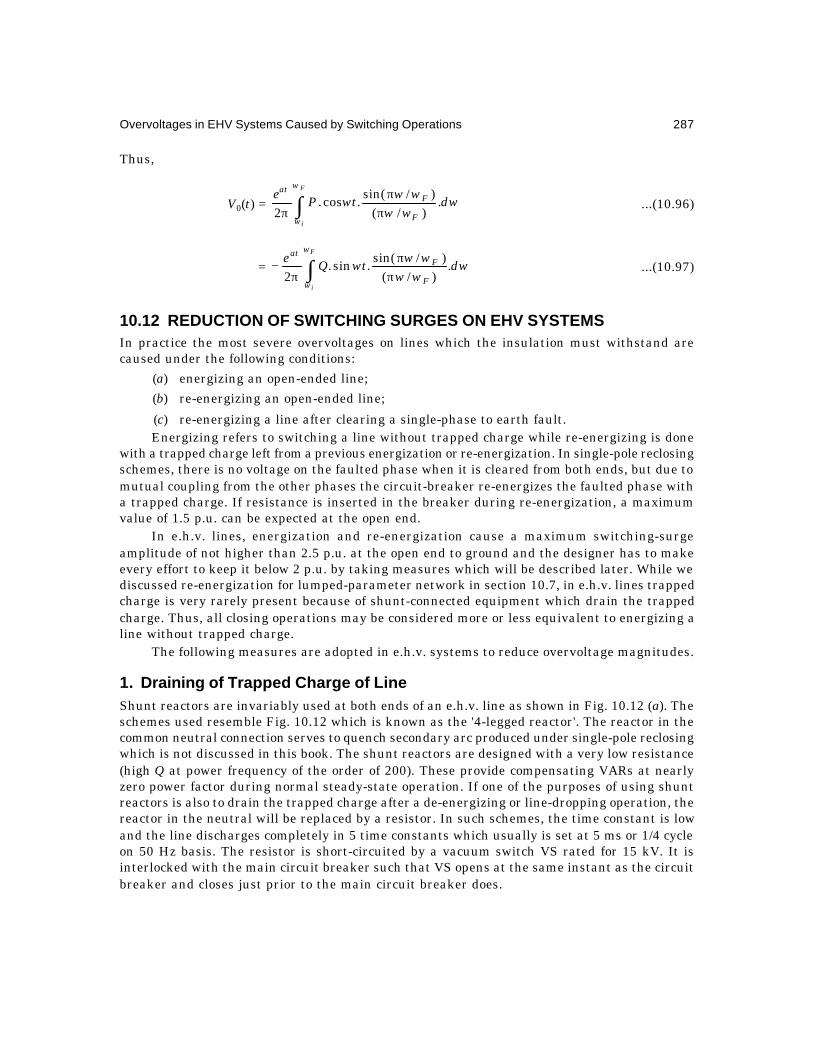
Overvoltages in EHV Systems Caused by Switching Operations 287
Thus,
V0(t) = ∫ ππ
π
F
i
w
w F
Fat
dwww
wwwtPe.
)/()/sin(
.cos.2
...(10.96)
= ∫ ππ
π−
F
i
w
w F
Fat
dwww
wwwtQe.
)/()/sin(
.sin.2
...(10.97)
10.12 REDUCTION OF SWITCHING SURGES ON EHV SYSTEMSIn practice the most severe overvoltages on lines which the insulation must withstand arecaused under the following conditions:
(a) energizing an open-ended line;
(b) re-energizing an open-ended line;
(c) re-energizing a line after clearing a single-phase to earth fault.Energizing refers to switching a line without trapped charge while re-energizing is done
with a trapped charge left from a previous energization or re-energization. In single-pole reclosingschemes, there is no voltage on the faulted phase when it is cleared from both ends, but due tomutual coupling from the other phases the circuit-breaker re-energizes the faulted phase witha trapped charge. If resistance is inserted in the breaker during re-energization, a maximumvalue of 1.5 p.u. can be expected at the open end.
In e.h.v. lines, energization and re-energization cause a maximum switching-surgeamplitude of not higher than 2.5 p.u. at the open end to ground and the designer has to makeevery effort to keep it below 2 p.u. by taking measures which will be described later. While wediscussed re-energization for lumped-parameter network in section 10.7, in e.h.v. lines trappedcharge is very rarely present because of shunt-connected equipment which drain the trappedcharge. Thus, all closing operations may be considered more or less equivalent to energizing aline without trapped charge.
The following measures are adopted in e.h.v. systems to reduce overvoltage magnitudes.
1. Draining of Trapped Charge of LineShunt reactors are invariably used at both ends of an e.h.v. line as shown in Fig. 10.12 (a). Theschemes used resemble Fig. 10.12 which is known as the '4-legged reactor'. The reactor in thecommon neutral connection serves to quench secondary arc produced under single-pole reclosingwhich is not discussed in this book. The shunt reactors are designed with a very low resistance(high Q at power frequency of the order of 200). These provide compensating VARs at nearlyzero power factor during normal steady-state operation. If one of the purposes of using shuntreactors is also to drain the trapped charge after a de-energizing or line-dropping operation, thereactor in the neutral will be replaced by a resistor. In such schemes, the time constant is lowand the line discharges completely in 5 time constants which usually is set at 5 ms or 1/4 cycleon 50 Hz basis. The resistor is short-circuited by a vacuum switch VS rated for 15 kV. It isinterlocked with the main circuit breaker such that VS opens at the same instant as the circuitbreaker and closes just prior to the main circuit breaker does.

288 Extra High Voltage AC Transmission Engineering
Instrument transformers such as the inductive type potential transformers (IPT) can alsodischarge the trapped line charge in contrast to capacitive voltage transformers (CVT). Powertransformers help to drain the trapped charge in about 20 ms or 1 cycle, if they are still leftconnected. But switching a transformer-terminated line is not looked with favour because ofthe possibility of ferro-resonance conditions. The Hydro-Quebec Company of Canada reliessolely on shunt rectors to keep the switching overvoltage to 2.1 p.u. on their 735 kV line andhave not equipped the circuit breakers with series resistances.
Fig. 10.12 (a) Four-legged reactor for draining trapped charge and quenching secondary arc during single-pole reclosing.
(b) Switching arrangement of series resistance in circuit breaker.MB–Main breaker. AB–Auxiliary breaker.
2. Series Resistance SwitchingFor lines of 400 kV and higher (or on some very long 220 kV lines also) reduction of switchingsurges to 2 p.u. or less can be attained by inserting a resistance R in series with the line. At thetime of energization, Fig. 10.12 (b), the main breaker is open while the auxiliary breaker
closes. The voltage impressed at the line entrance is thus Ve = )/().( 00 ZRZte + . If R = Z0, only50% of the source voltage is impressed on the line giving 1 p.u. at the open end due to totalreflection. Because the line is matched at the source end, the voltage settles down to thesource voltage very quickly. However, when re-energization with trapped charge occurs amaximum of 2 p.u. will be attained. Thus, with series-resistance switching the overvoltage isnever higher than 2 p.u. This has been verified by a large number of switching surge studiesusing the Transient Network Analyzer and Digital computer.
The value of resistance R in general depends on a large number of factors as follows:(a) The value of R is selected to achieve optimum results for the system.
(b) The surge impedance of connected lines when there is a single line or multiple lines.The lines switched might not all be of equal length so that complications arise due toreflections from the shorter lines getting into the longer ones and vice-versa.
(c) The insertion time of the resistance controls the overvoltage.
From a large number of studies, the following recommendations are made:
1. The insertion time is 8–10 ms or 21
cycle on 60 Hz or 50 Hz basis. After this time, the
resistance is shorted.
a b c
VS
( )a
MB
ABRs
V
( )b

Overvoltages in EHV Systems Caused by Switching Operations 289
2. The value of resistance is slightly higher than the surge impedance of a single linewhich is switched. In older designs a value of the order of 1000 ohms was used, butmodern practice is nearly 400 ohms.
3. The closing span of the circuit-breaker poles must be controlled within 60°.The last item is very important under 3-phase reclosing operations. Poorly-maintained
breakers can have a 180° lag between the first and last pole to close which result in highovervoltages since the last phase has a trapped voltage induced in it by the other phases whichhave already been energized. On the other hand, because of the non-synchronous or non-simultaneous closure of the poles with resulting unbalanced conditions, ground-return currentsare present which help to attenuate the surges. However, each case must be studied carefullyon models and the worst case guarded against.
3. Electronic Sensing of Voltage PolaritiesIn the resistance-insertion scheme the maximum overvoltage condition exists when the mainbreaker closes to short-circuit R in the auxiliary breaker, and at the same instant the polarityof line-side voltage is opposite to that of the source. Very sophisticated electronic circuitryusing sensors and logic elements to sense the polarities of the two voltages and to activate theclosing mechanism of the main circuit breaker exist. This connects the line directly to thesource while the polarities of voltages are the same. This applies when there is a trappedcharge on the line. In such schemes the overvoltage is brought down as low as 1.5 p.u. at theopen end. The scheme is improved further if the main breaker closes when the current in theline is zero when there are oscillations caused by the inductance and capacitance of the lineitself. Such a scheme has been developed and used successfully in the U.S.A. by the BonnevillePower Administration.
4. Limiting Value of Minimum Switching SurgeWhile a designer or user of such sophisticated and expensive equipment aims at lowering theovervoltages to 1.5 p.u. or less, it has been observed that there is not much advantage inlowering the overvoltage to less than 1.5 p.u. The main reason for this is that under a singleline to ground fault, the dynamic voltage rise is 1.5 p.u. or very near this value. For an 80%
arrester of the conventional type, the overvoltage under a fault reaches 4.138.0 = p.u.Therefore, there is not much advantage gained in lowering only the switching overvoltage.
However, with new gapless Metal Oxide arresters, the voltage rating of the arrester canbe as low as 60 to 65% of line-to-line voltage which permits a lowering of equipment insulationlevels. These arresters are meant for switching-surge duty so that e.h.v. insulation levels canbe brought down further.
10.13 EXPERIMENTAL AND CALCULATED RESULTS OFSWITCHING-SURGE STUDIES
We conclude this chapter with a discussion of switching-surge over-voltages as observed one.h.v. systems of typical configurations. These studies are carried out by three methods:
(a) Mathematical modelling using the Digital Computer,
(b) Physical modelling using the Transient Network Analyzer (TNA), and(c) Field Tests.

290 Extra High Voltage AC Transmission Engineering
Every designer involved in the selection of air-gap clearances or other types of insulationmust have exhaustive data on these two points:
(1) The expected maximum amplitudes of overvoltages at all points of all types in thesystem network, and
(2) The flashover or withstand voltages of the insulation structure to be selected whichwill insulate against the overvoltages.
Both these aspects are statistical in nature and involve application of probability theory.Some of these concerning insulation strength of long airgaps will be discussed in the nextchapter, Chapter 11.
The main factors to be investigated on a TNA or with a Digital Computer prior to linedesign are listed below. These vary with the system but the list covers the most importantitems used in e.h.v. systems.
1. Line Length L and Line Constants r, l, g, c: These quantities may not be trulyconstant because of the effect of frequency especially the ground-return parameters.In general, a frequency of f = 1/4T = v/4L can be used where v = velocity and T =travel time = L/v.
2. High Voltage Reactors: When these are depended upon to reduce the switching-surgemagnitudes by draining the trapped charge, the loss of one leg or as many legs as areanticipated must be studied. The loss of shunt reactor also raises the power-frequencyopen-end voltage due to Ferranti Effect. In lowering the switching-surge magnitudes,both the steady-state and transient components of voltage must be kept down.
3. Series Capacitors: The presence of series capacitors up to 50% line-inductancecompensation normally does not affect switching surges, but will affect the steady-state component in the total transient.
4. Short-Circuit Capacity of Source: This is reflected as the value of series reactance ofsource. In general, an infinite source (zero series impedance) yields higher switchingsurges at the open end of a line, but there are cases where this depends upon thelength of line switched as well as their number in parallel.
5. Damping Factor of Supply Network: The presence of ground currents on the switchingovervoltages plays an important role. The frequency-dependence of the zero-sequenceresistance and inductance must be properly taken into account in any study.
6. Presence of Transformers or Autotransformers: When a line is connected to a sourcethrough a transformer at the generating station, as is usual in unit-connected schemes,the line can be switched either on the high-voltage side or the low-voltage side. Ingeneral, when switched from the l.v. side the series-impedance of the transformerlowers the entrance voltage of the line and the switching over-voltage at the openend is lower than when switched from the h.v. side. The presence or absence oftertiaries has some effect on the switching surges.
7. Saturation of Transformers and Reactors: These give rise to harmonic oscillationswith the line capacitance.
8. Load Transmitted: A line-dropping operation followed by a fault due to the overvoltagegives very high surges if the circuit breakers at both ends do not open simultaneously.The power factor of load has considerable effect on the switching surges.

Overvoltages in EHV Systems Caused by Switching Operations 291
9. Single-Phase Reclosing: When a fault is cleared on a single line to ground fault byopening circuit breakers, due to mutual induction from the healthy phases, a currentof 20-30 Amperes keeps flowing in the arc at the fault on the grounded line. The deadtime, or the time interval between opening of the faulted line and its reclosure has tobe determined. With shunt reactors using 4-legged construction, the dead time is oforder of 5 seconds or 250-300 cycles.
10. Frequency of Source: This has only a secondary effect.11. Switching Resistors: These clearly have very important effect in reducing switching
overvoltages. The optimum values of resistance and the time of their insertion inseries with the circuit breaker has been the subject of intense study.
12. Order of Phases to Clear: Where circuit breaker poles have a time lag in closing oropening the switching-surge magnitude will have different value from simultaneousclosure called synchronous closing. The last phase to close has a higher overvoltagebecause of coupling of voltage from the other phases.
13. Restriking in Circuit Breaker: When breaker arcing chambers are unable to interruptproperly, there is a restrike which essentially connects a line to the source withtrapped charge on the line. This has been considered in section 10.5. Long linescause maximum trouble due to line dropping with restrike in circuit breaker causinglightning-arrester failures or circuit-breaker explosions due to frequent operation.
14. Lightning Arrester Sparkover Characteristics: These are normally set for 1.5 p.u.with gap type SiC arresters. If magnetic blowout or current-limiting gaps fail, thenthey cannot handle switching surge duty. Their effect on insulation levels must beinvestigated.
15. Line-to-line Voltages: In order to design conductor-to-conductor clearances, a knowledgeof phase-to-phase overvoltage magnitude is necessary. It is insufficient to obtain themaximum expected line-to-ground voltage on one phase and multiply by 3 . Themaximum is lower than this value because of the waveshapes not being sinusoidal.
Out of an enormous amount of studies carried out all over the world, the following typesof conditions leading to overvoltages are considered very important. Against each item, a list ofparameters which affect the overvoltage is given.
1. Interruption of Line at No Load : Length of line, line constants, shunt reactors, seriescapacitors, reactance of source, and switching resistors.
2. Load Shedding: All of the above factors and in addition saturation effects oftransformers and reactors, load characteristics and damping factors.
3. Load Shedding at End of Line Followed by Disconnection of Unloaded Line: All of theabove factors plus natural frequency of supply network as it affects the restriking inthe breaker.
4. Clearing a Short Circuit: All the above factors.5. Closing a Transformer-Terminated Line with Load: All the above factors plus order of
phases to close which causes possible ferro-resonance condition.
6. Energizing or Re-energizing an Unloaded Line: All the above factors minus thetransmitted load.
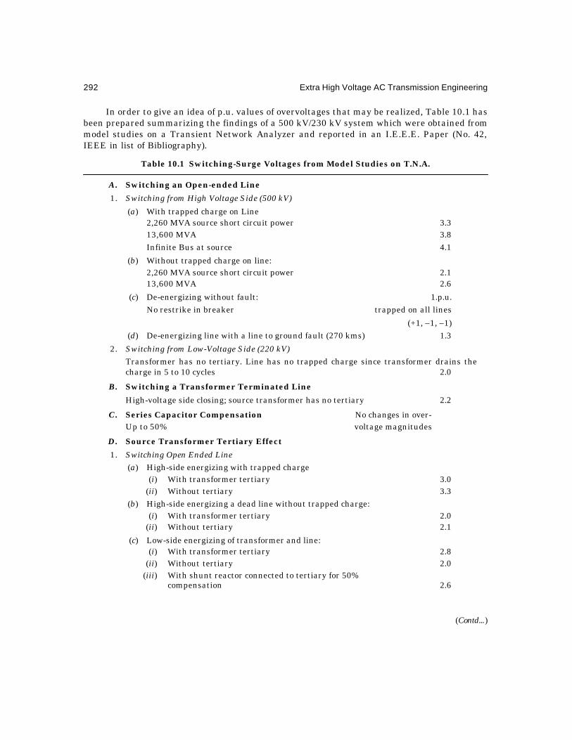
292 Extra High Voltage AC Transmission Engineering
In order to give an idea of p.u. values of overvoltages that may be realized, Table 10.1 hasbeen prepared summarizing the findings of a 500 kV/230 kV system which were obtained frommodel studies on a Transient Network Analyzer and reported in an I.E.E.E. Paper (No. 42,IEEE in list of Bibliography).
Table 10.1 Switching-Surge Voltages from Model Studies on T.N.A.
A. Switching an Open-ended Line
1. Switching from High Voltage Side (500 kV)
(a) With trapped charge on Line2,260 MVA source short circuit power 3.313,600 MVA 3.8Infinite Bus at source 4.1
(b) Without trapped charge on line:2,260 MVA source short circuit power 2.113,600 MVA 2.6
(c) De-energizing without fault: 1.p.u.No restrike in breaker trapped on all lines
(+1, –1, –1)(d) De-energizing line with a line to ground fault (270 kms) 1.3
2. Switching from Low-Voltage Side (220 kV)Transformer has no tertiary. Line has no trapped charge since transformer drains thecharge in 5 to 10 cycles 2.0
B. Switching a Transformer Terminated Line
High-voltage side closing; source transformer has no tertiary 2.2
C. Series Capacitor Compensation No changes in over-Up to 50% voltage magnitudes
D. Source Transformer Tertiary Effect
1. Switching Open Ended Line(a) High-side energizing with trapped charge
(i) With transformer tertiary 3.0(ii) Without tertiary 3.3
(b) High-side energizing a dead line without trapped charge:(i) With transformer tertiary 2.0
(ii) Without tertiary 2.1
(c) Low-side energizing of transformer and line:(i) With transformer tertiary 2.8
(ii) Without tertiary 2.0(iii) With shunt reactor connected to tertiary for 50%
compensation 2.6
(Contd...)

Overvoltages in EHV Systems Caused by Switching Operations 293
E. Lightning Arrester
Arrester at sending end set to spark at:(a) 2.0 p.u. 3.0(b) 1.5 p.u. 2.6
Arrester included at receiving end, and set to sparkat 1.5 p.u. 2.2
F. Surge Suppressing Resistor in Breaker
In all cases where overvoltages exceeded 2.3 p.u.,1200 ohms was included 2.0
G. High Speed Reclosing After Fault Clearing(with trapped charge) 3.6
H. Effect of Non-Synchronous Operation of Circuit Breaker Poles(a) Breaker poles close within 1/2 cycle 2.4(b) Breaker poles close on 1 cycle 3.5
Review Questions and Problems
1. A 750 kV system has a generation of 4000 MVA. The transient reactance of thesource is 0.25 p.u. on 750 kV 4000 MVA base and the unit-connected transformer hasa leakage reactance of 0.15 p.u. For a 3-phase bus fault on the high-voltage side of thetransformer, calculate the short-circuit current in kiloamperes and in p.u.
2. Explain the term s (a) sub-transient reactance, (b) transient reactance, (c) synchronousreactance of a source, and (d) a.c. component, (e) d.c. component, and (f) theinterrupting current capacity of a circuit breaker.
3. Explain the terms (a) terminal fault, (b) short-line fault, (c) 2-parameter definition ofrecovery voltage, and (d) 4-parameter definition of recovery voltage.
4. Explain clearly how overvoltages are generated when interrupting (a) low inductivecurrents and (b) low capacitive current. Draw a figure showing ferro-resonancecondition in a network when two poles of a circuit breaker are open and one pole isclosed.
5. A series L-R-C circuit has a L = 0.3 H, R = 9 ohm, and C = 3.3 µF. It is excited by astep input of magnitude 600 kV with the initial value of capacitor voltage equal to–600 kV, in Fig. 10.7. Calculate the following–
(a) attenuation factor LR 2/=α , (b) the natural frequency of oscillation w0 and f0.(c) the first peak of voltage across the capacitor, (d) the ratio of adjacent positivepeaks of voltage from zero value.
6. Repeat problem 5 if the resistance is increased to the value R = CL /2 . Only parts(a) and (c) apply.

294 Extra High Voltage AC Transmission Engineering
7. A 750 kV 500 km 50 Hz line has the following details;
Conductor resistance, rc = 0.03 ohm/km;Ground return resistance, rg = 0.27 ohm/km at 100 Hz;
Series line inductance, ls = 0.9 mH/km;
Ground return inductance, lg = 0.6 mH/km;
Shunt capacitance, c = 12.33 nF/km.
Working on single-phase basis, calculate the following with and without consideringground-return parameters:
(a) Velocity of propagation and travel time;
(b) Surge impedance Z0 and attenuation factor LReA T 2/,0 =αα−= .
(c) Plot the step response upto 20 ms when the voltage of 1 per unit is switched on tothe line suddenly. Neglect trapped charge.
(d) Plot the response upto 20 ms when the sinusoidal voltage of 3/750 kV to groundis switched on to the line at (i) positive peak, and (ii) 30° after the positive peak.Neglect trapped charge in both cases.

11.1 TYPES OF ELECTRODE GEOMETRIES USED IN EHV SYSTEMSIn e.h.v. transmission systems, other than the internal insulation of equipment such astransformers, circuit breakers, etc., all external insulation is air at atmospheric pressure andelectronegative gases such as SF6. Air gaps used for insulation have now reached enormouslengths—up to 20 metres and more—and will increase with further increase in transmissionvoltage. As of this date, the highest commercially-used voltage is 1200 kV, ac. But experimentalprojects at 1500 kV ac have been in progress since 1980. It is very important and vital to knowthe breakdown and withstand properties of such long gaps and in this chapter we will discussonly air gaps.
The insulation characteristics of long air gap lengths namely the flashover and withstandvoltages are governed mainly by the geometry of the electrodes insulated by the gap. The mostusual electrode geometries are shown in Figure 11.1. Representative air-gap lengths used inconductor-to-tower gaps are:
400 kV 500 kV 750 kV 1000 kV 1150-1200 kV2.134 m 2.59 m 5.6 m 7 m 8 m (U.S.A.)(84") (102") 10 m (U.S.S.R.)
These gaps are subjected to several types of voltage waveshapes so that breakdown andwithstand voltages have to be ascertained for all of them. These are:
(a) Power Frequency A.C.; (b) Lightning Impulses—positive and negative; (c) SwitchingSurges—positive and negative; (d) D.C.—positive and negative; and (e) A.C. with a D.C. offset.
In both indoor and outdoor high-voltage laboratories, experiments at great expense havebeen and are being conducted in order to determine the breakdown voltages of air-gap geometries.Along with these important experiments, a very large amount of theoretical work concerningthe basic mechanisms of breakdown have also been handed down in technical literature. Oncethese mechanisms are thoroughly understood, the breakdown characteristics of very long airgaps have been known to follow the same pattern as small gaps. An understanding of basicbreakdown mechanisms helps to reduce the expense involved in large-scale experiments andproper interpretation of such experimental results.
All breakdown phenomena depend on the electric field distribution in the gap which initiatesthe primary electron-avalanche mechanism, leading to secondary mechanisms, as these dependon the velocities or energies of the resulting ions. In very long gaps, especially under switching
11Insulation Characteristics of Long Air Gaps
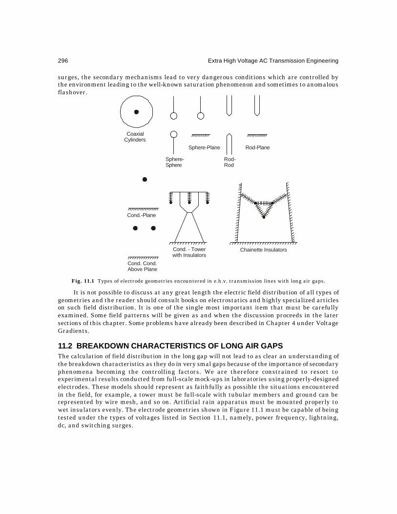
296 Extra High Voltage AC Transmission Engineering
surges, the secondary mechanisms lead to very dangerous conditions which are controlled bythe environment leading to the well-known saturation phenomenon and sometimes to anomalousflashover.
Fig. 11.1 Types of electrode geometries encountered in e.h.v. transmission lines with long air gaps.
It is not possible to discuss at any great length the electric field distribution of all types ofgeometries and the reader should consult books on electrostatics and highly specialized articleson such field distribution. It is one of the single most important item that must be carefullyexamined. Some field patterns will be given as and when the discussion proceeds in the latersections of this chapter. Some problems have already been described in Chapter 4 under VoltageGradients.
11.2 BREAKDOWN CHARACTERISTICS OF LONG AIR GAPSThe calculation of field distribution in the long gap will not lead to as clear an understanding ofthe breakdown characteristics as they do in very smal gaps because of the importance of secondaryphenomena becoming the controlling factors. We are therefore constrained to resort toexperimental results conducted from full-scale mock-ups in laboratories using properly-designedelectrodes. These models should represent as faithfully as possible the situations encounteredin the field, for example, a tower must be full-scale with tubular members and ground can berepresented by wire mesh, and so on. Artificial rain apparatus must be mounted properly towet insulators evenly. The electrode geometries shown in Figure 11.1 must be capable of beingtested under the types of voltages listed in Section 11.1, namely, power frequency, lightning,dc, and switching surges.
CoaxialCylinders
Sphere-Sphere
Cond.-Plane
Rod-Rod
Sphere-Plane Rod-Plane
Chainette InsulatorsCond. - Towerwith Insulators
Cond. Cond.Above Plane

Insulation Characteristics of Long Air Gaps 297
The most important factors by which engineers describe the breakdown voltage are thewithstand voltage and critical flashover voltage or 50% flashover voltage which is the voltagethat yields flashover in 50% of the number of shots given to the air gap. The withstand voltageis based on probability basis and will be explained later on. The following empirical relationsbetween the CFO (50% flashover voltage) and gap length are valid for design purposes forpositive-polarity voltages, except for ac excitation. All voltages are peak values of voltage,including power frequency. Negative polarity flashover, except under rain under switchingsurges, will always be higher than positive polarity or become equal to it. Under exceptionalcircumstances, such as in heavy rain under switching surges, it may be lower than positive-polarity flashover.
Switching SurgeLightning D.C. Power Frequency (120/4000 sµ )Rod-Plane: Gap Length in metres, V50 in kV crest1.2/50 µs–550d 500d 652d0.576 535.5d0.552(3<d<9)
1/50 - 667d 500d0.6
Rod-Rod
1.2/50µs–580d 555d 500d 872d0.429
687d0.6
For positive-rod negative-plane electrodes, the following additional formulas are also inuse.
Feser's FormulasStatic voltage: 500d + 12, kV (d in metres) ...(11.1)Power Frequency: 455d + 25 ...(11.2)1.2/50 sµ Lightning: 540d ...(11.3)Switching Surge: 250150100 −+d ...(11.4)
Leroy and Gallet Formula
Switching Surge 3400/(1 + 8/d) ...(11.5)
Paris et al. Switching surge – 500d0.6 or 535d0.552 ...(11.6)All the above formulas, are based on experimental results and are compared in Figure
11.2. There are however, many attempts made from time to time to derive a theoretical expressionfor the sparkover voltage
Fig. 11.2 Comparison of flashover characteristics of long air gaps under lightning impulse ),50/2.1( sµdc, power frequency (PF), and positive switching surges.
6000
4000
2000
00 2 4 6 8 10 17
V s, k
V
1.2/50 sµ DC
PF
S.S. (+)
d, metres

298 Extra High Voltage AC Transmission Engineering
in terms of the basic physical processes that might be occurring in long gaps. They arebased on the following broad assumptions:
(1) Prior to breakdown, there exists an intense corona envelope on the highly-stressedelectrode. This is particulary prominent on the positive rod in a rod-plane arrangementand on both rods in a rod-rod air gap. This spherical corona envelope is assumed tohave a diameter ranging from 20 cm to 1 metre.
(2) The corona gives rise to leader channels of about 1-3 mm in diameter such that theradial electric field is 20 kV/cm with a charge of about 0.5 to 1 .cm/cµ These leadersfork out in all directions but one that eventually causes the sparkover propagatesalong the axis of the gap and is preceeded by a leader-corona at its tip. The axialelectric field in the leader column is about 5 kV/cm.
(3) When the leader corona has reached a length of 4.5 to 5 metres in a 7 m gap, or about65–70% length, the influence of the plane cathode is so intense that there results ajump-phase where the acceleration of the leader corona is high enough to bridge theremaining portion of the gap. In a rod-rod gap, a negative-leader propagates from thenegative rod also to meet the positive leader and sparkover occurs.
Without going through the derivation of the following equations which are based on differingassum ptions, three expressions are given for the 50% sparkover voltage, Vs, for positive switchingsurges in terms of the gap length, d.
I. Lemke's Model. (d < 10 m)
Vs = kV)],ln(ln33.11[450 dd −+ ...(11.7)
II. Waters' Model
Vs = kV,350)102.3105.1( 5.056 −×+× d ...(11.8)
III. Alexandrov's Model, )m9.0( =r
Vs = kV,/1tanh.)/1(1260 15.0 drdrr −− − ...(11.9)All of the above three models yield nearly the same value of Vs for gap length up to 20 m.
It is therefore very surprising how widely differing assumptions made by the three investigatorscan lead to close results. They also correspond very closely to the empirical formulas of Leroyand Gallet, and Paris et al. Results of comparison of these models are shown in Figure 11.3.
Fig. 11.3 Comparison of CFO vs gap length according to the models of Lemke (LK), Waters (WT),and Alexandrov (AL).
ALWTLK
3000
2000
1000
00 4 8 12 16 20
V s, k
V
d, metres

Insulation Characteristics of Long Air Gaps 299
11.3 BREAKDOWN MECHANISMS OF SHORT AND LONG AIR GAPSLiterature describing the physical mechanism of sparkover of gaps is immense and varied. Wewill only give the broad outline here of several basic and important theories which have beenput forward by eminent physicists and engineers to give the design engineer an indication ofsome of the physical processes in uinderstandable terms. It is recognized by all that acomprehension of these basic mechanisms of sparkover will help to design experiments ofbreakdown involving less expense and time.
We limit ourselves to the mechanism of gaps near atmospheric pressure. The two classictheories of breakdown of small gaps with uniform fields are the well-known: (1) Townsend andRaether mechanisms called the avalanche theory, and (2) the streamer theory of Loeb andMeek. After discussing these two theories, we will briefly outline the several theories or modelsof breakdown of long gaps put forward by many workers to explain the dependence of the 50%breakdown voltage with change in gap length, which in one way or another are based on theavalanche and streamer theories of uniform field gap breakdown.
11.3.1 Townsend's Theory and Criterion of SparkoverFigure 11.4(a) shows a uniform-field gap between an anode and a cathode with E = V/d. Aninitial free electron in the gap acquires sufficient energy to release further electrons from theintervening gas molecules to cause an electron avalanche. It is evident that if the electric fieldis high the electrons cause increased ionization within limits while with increase in gas pressure,p, the number of molecules or density of gas is increased so that the free path of an electron isdecreased before another collision can occur. This results in an electron acquiring low velocityand kinetic energy between collisions, and the probability that it will release another electronfrom a gas molecule is reduced. The effect of electric field intensity E and the gas pressure p onthe probability of creating new electrons by an incident electron on gas molecules is thereforeproportional to E and 1/p. This is expressed through Townsend's first ionization coefficient, .α
Fig. 11.4 (a) Theory of avalanche breakdown of uniform-field gap (Townsend and Raether)(b) Theory of streamer breakdown (Loeb and Meek).
Thus,α = mean number of collisions taking place in 1 cm of drift by 1 electron. ...(11.10)The value of α is determined experimentally and has the following characteristics in
Nitrogen, where n = number density of molecules at the given temperature and pressure[n = 2.69 × 10¹⁹/cm3 at 0°C and 760 mm].
Vd
Ep
Anode +
Cathode –
–
++
( )a ( )b
++++++
–
++
Anode +
V
V
p
E
E3
E2
E1
Cathode –

300 Extra High Voltage AC Transmission Engineering
E/n 100 200 300 400 500 600n/α 10–19 4 × 10–18 1.5 × 10⁻¹⁷ 3 × 10–17 4.5 × 10⁻¹⁷ 5 ×10–17.
The best fit for this variation (carried out by the author) gives a formula of the type
)/(log10 nα = ]1)//(74.16/[82.15 −nE ...(11.11)
The ion density can be converted to pressure of gas by the relation.
n = )/273).(760/(1069.2 19 TpT× ...(11.12.)
where pT = pressure of gas in mm Hg at temperature T °K. Then, at 20°C (T = 293 °K),n = 3.295 ×10¹⁶ p20. This gives
α = θ10.5 .20p ...(11.13)
where θ = )10516.5//(108725.0 1720
19 ×−× pE ...(11.14)
This shows that α = p.f1 (E/p) where f1 (E/p) is a function of (E/p) only.A single avalanche is attracted by the positive electrode because of the intense negative
charge at its head, at a velocity of about 107 cm/sec, whereas the drift velocity of positive ionsleft behind and travelling towards the cathode is about 105 cm/sec since they are much heavierthan electrons. Thus, the cloud of positive ions is almost stationary as compared to the drift ofthe electron avalanche. The positive ions, however, disturb the electric field due to the spacecharge.
The single electron avalanche reaching the anode does not constitute sparkover since thegap is not completely bridged by electrons to constitute a heavy enough current flow. Thebreakdown or sparkover of the gap occurs due to a succession of avalanches generated bysecondary mechanisms caused by the primary-avalanche electrons. These are (a) thermionicemission from the cathode due to the high energy acquired by the positive ions or unstableneutral molecules; (b) excited molecules emitting photons on returning to the ground statewhich will cause photo-emission of electrons; (c) the potential of the positive-ion space chargenear the cathode being sufficient to eject electrons upon striking the cathode. In whatevermanner these are released, the number of electrons now increases due to secondary mechanismsand is described by Townsend's second ionization coefficient .γ Once again (like α) γ is a functionof (E/p). From available experimental results, the author has found that the functionalrelationship between γ and (E/p) is of the type
γ = 66.13466.16 )/(10782.5)/(1052.1 pEnE −− ×=× ...(11.15)
The current intensification due both to the primary and secondary mechanisms is, whenthe avalanches cross the gap distance d,
α-process only: I = deI α.0 ...(11.16)
γ-process also: I = )]1(1/[.0 −γ− αα dd eeI ...(11.17)
The Townsend criterion for spark breakdown is taken as ,∞→I or when the denominatorof equation (11.17) becomes zero, that is,
)1( −γ αde = 1 ...(11.18)
Since the functional relationship of α and γ with gas pressure p and electric field intensityE is known, the value of (E/p) is calculated by trial and error from equation (11.18). In the

Insulation Characteristics of Long Air Gaps 301
uniform field, E = Vs /d so that the value of (Vs /pd) is found, and the sparkover for given valuesof p and d can be calculated.
11.3.2 Paschen's LawUsing )/( and)/(. 21 pdVfpdVfp =γ=α for a uniform-field gap, the Townsend breakdown criterionof equation (11.18) can be re-written as
1]1)./().[exp/( 12 =−pdpdVfpdVf ss ...(11.19)
Thus, the sparkover voltage Vs is a function of (pd), which is Paschen's Law. In air, theformula for sparkover voltage is found to be
Vs = kV,760
.273
2027308.6
760.
27320273
.22.24pd
tpd
t +++
++
= kV,/775.3/34.9 TpdTpd + ...(11.20)
where p is in mm Hg, d in cm, and t in °C.
The above relation holds even for gases with electron attachment such as SF6, whoserelative electric strength compared to air is 2.5/1.
At standard temperature and pressure, equation (11.20) gives the uniform-field sparkoverfor 1 cm gap as 30.3 kV.
In non-uniform fields such as co-axial cylindrical geometry and cylinder-cylinder (conductor-conductor on a transmission line) gaps, F.W. Peek, Jr., has determined the following expressionsfor onset of partial discharge (corona) in the highly divergent field distribution for air-densityfactors close to unity.
Concentric Cylinders. E0 = peakcm,/),/308.01(31 kVrδ+δ ...(11.21)
Parallel Cylinders. E0 = peakkV/cm,),/301.01(30 δ+δ r ...(11.22)
Here, r = radius of inner cylinder or conductor in cm,
and δ = air-density factor ,/3856.0760
.273
20273 Tppt
=+
+= ...(11.23)
with p = pressure in mm Hg.
The pressure varies with temperature and altitude as described in Chapter 4. See Problem4 at end of Chapter 4.
11.3.3 Streamer Breakdown Theory of Loeb and MeekIn the Townsend mechanism, the time lag of breakdown, which is the time interval betweenapplication of potential and the breakdown of the gap, is equal to the transit time of the electronavalanche. However, it has been observed with long air gaps in uniform fields, in practice, thattime lags are shorter than those postulated by electron-transit times. This has led to theStreamer Theory of breakdown. It uses the property that a very high concentration of theelectric field occurs in front of the electron-avalanche head, as well as in the space between thepositive-charge cloud and the cathode. These two are directed in the same sense as the applied

302 Extra High Voltage AC Transmission Engineering
electric field as shown in Figure 11.4(b). In the space between the electron-avalanche head andthe positive space-charge cloud the field is lower than the applied uniform field. Thephotoelectrons emitted in the augmented field initiate auxiliary avalanches, which are intensealong the axis of the main avalanche, will be directed towards the anode to be absorbed there.The positive ions then form a self-progagating streamer extending from the anode to cathodeforming a conducting plasma. This constitutes the breakdown of the gap.
Loeb and Meek considered the transition from electron avalanche to streamer to occurwhen the field produced between the positive ions and the avalanche head is equal to theapplied field E = V/d. The breakdown criterion obtained by them, with a spherical avalanchehead, can be written as
Vs = pded d //).(1027.5 )(7 α− α× ...(11.24)
Since ),/(. 1 pdVfp s=α the sparkover voltage is once again a function of (pd). The equationcan be solved for Vs for given values of p and d by trial and error. The functional relationshipbetween α and (Vs /pd) is of the type of equation (11.13).
11.4 BREAKDOWN MODELS OF LONG GAPS WITH NON-UNIFORM FIELDSAs mentioned earlier, several models for explaining the observed characteristics of the 50%breakdown of long air gaps have been put forward from time to time. The main characteristicsof gap sparkover which need to be explained by any of the models are listed below:
(1) The functional relationship between sparkover voltage and gap length for a givenelectrode geometry. Most theories confine themselves to a rod-to-plane gap, and tryto evolve a factor called the "gap factor" to extend the equation to apply to other typesof gap geometries found in practical engineering situations, usually obtained as aresult of experimental observations.
(2) The volt-time characteristics which produce the time lag for breakdown afterapplication of the voltage to the gap.
(3) The relation between switching-surge front time and the sparkover voltage calledthe U-characteristic.
(4) The average electric field in the gap at the instant of breakdown.
(5) The charge in the leader column and its velocity of propagation, as well as the size ofcorona envelope around the highly-stressed electrode (rod).
(6) Some other characteristics which are governed by the convergent or divergent electricfields.
None of the models put forward so far in technical and scientific literature consider all theabove factors in one model nor the complete mechanism of distribution of the charge, thetemperature, the velocity, number density, column radius, leader-corona size, microscopicvoltage gradient, etc. Some theories or models use experimental data to obtain numericalestimates for the salient governing factors, as will be outlined below. We will first list thecommon factors to all theories and then point out where they differ, and yet in the final resultthey all show agreement among each other within limits.
The mechanism of breakdown depends on a leader or streamer propagating from the rodanode towards the plane cathode in a rod-plane gap with the rod positive. The onset of this
Insulation Characteristics of Long Air Gaps 303
"positive leader" is preceded by an initial corona discharge, and also accompanied by corona atthe leader tip. This leader carries a current of less than 1 Ampere and propagates at a velocityvarying from 1 to 10 cm/ .sµ When the leader corona approaches the plane-cathode, secondaryprocesses give rise to a streamer which meets the leader in most cases, that is, there is a"jump-phase" in which conditions are ripe for the latter portion of the leader to reach the anodeat velocities exceeding 100 cm/ .sµ Once the gap is bridged, a return current stroke from theplane cathode follows in the ionized channel whose velocity can reach 300 cm/ sµ *. The potentialgradient in the return stroke is of the order of 1 kV/cm or more.
Pre-breakdown streamer pulses in the corona are followed by break-down streamers. Thecharge in the leader channel varies from 0.5 C/cmµ to 4 C/cmµ depending on the resistanceconnected in series with the gap to the source, and the waveshape of the applied impulsevoltage. The corona envelope at the rod gives rise to 50 or more leader branches out of whichonly one causes the streamer breakdown. The rest give rise to leader-tip coronas which causephoto-ionization of the gap and help secondary processes. The temperature of the leader hasbeen known to exceed 5000 °K and the longitudinal electric field approaches 2–3 kV/cm. Thecorona envelope has been known to extend to diameters ranging from 20 cm to 2 metresdepending upon the overvoltage. For small gaps, the space charge in the corona envelopelowers the electric field in the gap to such an extent that large voltages for breakdown arerequired. This effect is less pronounced as the gap length increases so that breakdown voltagesless than suggested by a linear increase are indicated. The entire phenomenon is thereforenon-linear with the breakdown voltage showing a lower increase with gap spacing for switchingsurges ).( 6.05.0 −∝ dVs Since most of these conditions are governed by the waveshape of theapplied voltage, several factors governing the sparkover voltage have to be measured underactual conditions in the laboratory from smaller gaps in order to predict the breakdowncharacteristics of very long gaps.
We will now consider a few important models.
(a) Lemke's Model
The simplest and a very straight-forward model is due to Lemke, which is based on certaincontradictory assumptions as pointed out by Waters (see Meek and Craggs, (ed), ElectricalBreakdown of Gases, Chapter 5, 1978). It takes into account the properties of two componentsin the leader channel: (i) a leader length L1. and (ii) a leader-corona discharge tip of length Lt
with potential gradient Et. Sparkover condition is assumed to reach when ,1 dLL t =+ the gaplength. The sparkover voltage is
Vs = tt LELE .. 11 + ...(11.25)
It is the determination of the four controlling quantities that give rise to some problems.The potential drop along the leader turns out to be
V1 = )/1ln(... 010011 LLLELE += ...(11.26)
where E0 = 1.5 kV/cm chosen by Lemke which is felt low,and L0 = 1 m from photographs taken of the leader propagation in gaps up
to 2m.
*Velocity of light = 0.3 km/µs = 300 m/µs = 30,000 cm/µs.
304 Extra High Voltage AC Transmission Engineering
Turning to the leader-corona tip, the potential gradient Et in the streamers of the leader-7corona is assumed to be 4.5 kV/cm based on observations made with 1 m gap. The length ofthe streamers, Lt, is also obtained from measurements and is
Lt = 1 + ln d ...(11.27)Finally, the critical sparkover voltage comes out to be
Vs = cm,in)],ln(ln)./1(1[ 0 dddEEE tt −++
= 450 [1 +1.33 ln (d –ln d)], kV. ...(11.28)This formula yields values of Vs which agree with experimental results for switching-
surge flashovers up to gap lengths of 10 m, but lower values for larger lengths. Therefore, gapclearances required beyond 10 m will be larger than required when using this formula and willgive uneconomical designs. However, it is worthwhile mentioning at this stage that up to 1150kV transmission, external insulation using air gaps on towers are not in excess of 9 metres andthis simple model is adequate.
(b) Waters' and Jones' Mechanism
In this model, a critical length for the leader propagation is postulated which if attained, a largeincrease in current takes place and sparkover results. The calculation of the critical leaderlength is attempted. In a rod-plane gap, the average potential gradient in the leader channel isgoverned by the degree of ionization given by Saha's equation through the channel temperaturewhich is caused by i2 R heating. Because of this heat and increased ionization, the averagepotential gradient in the leader channel is increased from 3–4 kV/cm to a value of about10 kV/cm when the leader reaches 24 cm length in a 2-metre rod-plane gap. If the leaderpropagates beyond this length, due to still higher ionization (and possibly due to intensesecondary mechanisms) the average voltage gradient falls to 1–2 kV /cm very quickly andsparkover occurs.
The model does not give a specific relation between sparkover voltage and gap length, butgives the mean potential gradient in the leader during the decreasing gradient process to be
E1 = kV/cm),25.51.()(25.1 85/2/1 tei −− + ...(11.29)
where t is in .sµ The current i in most cases is equal to 0.75 A but is related to thetemperature.
(c) Alexandrov's Model
In this theory, three quantities are assumed to govern the breakdown: (1) the leader-tip potential,(2) electric field strength at the head of the developing discharge, and (3) radius of curvature ofthe tip. The relation among them is found by Alexandrov to be
Vt = drdrrE t /1tanh./1.. 1 −− − ...(11.30)
where Vt = leader-tip potential,Et = electric field gradient at the head of the developing discharge,
and r = radius of curvature of the tip = 0.9 metre.The value of Et was obtained experimentally, while r was calculated to be 0.91 m for a 2-
m gap and 0.98 for a 30-m gap. For sparkover condition, Et = 12.6 kV/cm =1260 kV/m. Therefore,

Insulation Characteristics of Long Air Gaps 305
equation (11.30) for the sparkover voltage becomes.
Vs = drdrr /1tanh./11260 1 −− − ...(11.31)
(d) Waters' ModelAnother model proposed by Waters assumes that the current flow in the positive leader column,i, depends upon the tip potential Vi in a parabolic manner, as derived by Townsend. The unbridgedgap between the leader tip and plane cathode is assumed to break down when the leader-tippotential is (0.5 V + 175) kV, where V = anode potential. From this, and other experimentalobservations that the leader length is 20 cm in a 2-m gap at 1000 kV, the sparkover voltagederived by Waters is
Vs = kV350]105.3105.1[ 2/156 −×+× d ...(11.32)
Another expression derived by Waters from certain observations made of the basicprocesses by the team from Electricite' de France is, with d in metres,
Vs = kV,.563 5.0d ...(11.33)
With all these models based on differing assumptions, it must be clear that a unifiedmodel can be attempted by a research worker even today.
11.5 POSITIVE SWITCHING-SURGE FLASHOVER—SATURATIONPROBLEM
In selecting the required air-gap insulation clearance for e.h.v. towers between the conductorand tower structure, its ability to withstand positive switching surges with condcutor positiveis of paramount importance. The shortest air gap occurs in the tower window and has been thesubject of intensive investigation. The problem is complicated since the critical flashover voltagedepends upon (a) the wave-front time of the switching surge, (b) the gap length, (c) the width ofthe tower structure, and (d) the presence of insulator and other hardware. Therefore, no twolaboratories agree on the CFO voltage of a given gap length in a conductor-to-tower insulationstructure. From a very large number of experimental results available, some importantobservations and properties are worth noting.
(1) The CFO voltage V50 of tower windows with insulator strings inside them varies withthe front-time of the switching surge. Typical flashover voltages are shown in Figure11.5 [Menemenlis and Harbec. See No. 56, IEEE, in Bibliography].
(2) The CFO voltage varies with the percentage of space filled by porcelain of the insulatorstring which has a higher permittivity than air.
(3) The CFO voltage depends upon the ratio of the shortest distance in air betweenconductor and tower (the "strike distance") to the length of the porcelain or glassinsulator string. A ratio between 0.85 and 1 is normally used in tower windows.
(4) The first switching-surge tests performed by J.W. Kalb, Jr., of the Ohio Brass Co.,U.S.A., established the important property that the minimum value of CFO occurredat a certain front time. His experiments for 525 kV towers with 24 insulators in thestring gave the minimum CFO at a wave-front time of 250 .sµ The CFO was higherat shorter and longer wave-front times than this value.
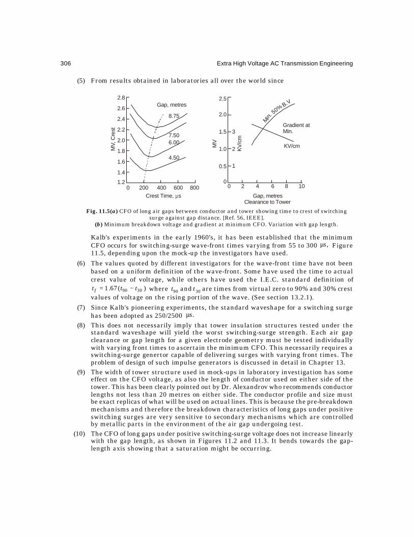
306 Extra High Voltage AC Transmission Engineering
(5) From results obtained in laboratories all over the world since
Fig. 11.5(a) CFO of long air gaps between conductor and tower showing time to crest of switchingsurge against gap distance. [Ref. 56, IEEE].
(b) Minimum breakdown voltage and gradient at minimum CFO. Variation with gap length.
Kalb's experiments in the early 1960's, it has been established that the minimumCFO occurs for switching-surge wave-front times varying from 55 to 300 ,sµ Figure11.5, depending upon the mock-up the investigators have used.
(6) The values quoted by different investigators for the wave-front time have not beenbased on a uniform definition of the wave-front. Some have used the time to actualcrest value of voltage, while others have used the I.E.C. standard definition of
)(67.1 3090 tttf −= where 3090 and tt are times from virtual zero to 90% and 30% crestvalues of voltage on the rising portion of the wave. (See section 13.2.1).
(7) Since Kalb's pioneering experiments, the standard waveshape for a switching surgehas been adopted as 250/2500 .sµ
(8) This does not necessarily imply that tower insulation structures tested under thestandard waveshape will yield the worst switching-surge strength. Each air gapclearance or gap length for a given electrode geometry must be tested individuallywith varying front times to ascertain the minimum CFO. This necessarily requires aswitching-surge genertor capable of delivering surges with varying front times. Theproblem of design of such impulse generators is discussed in detail in Chapter 13.
(9) The width of tower structure used in mock-ups in laboratory investigation has someeffect on the CFO voltage, as also the length of conductor used on either side of thetower. This has been clearly pointed out by Dr. Alexandrov who recommends conductorlengths not less than 20 metres on either side. The conductor profile and size mustbe exact replicas of what will be used on actual lines. This is because the pre-breakdownmechanisms and therefore the breakdown characteristics of long gaps under positiveswitching surges are very sensitive to secondary mechanisms which are controlledby metallic parts in the environment of the air gap undergoing test.
(10) The CFO of long gaps under positive switching-surge voltage does not increase linearlywith the gap length, as shown in Figures 11.2 and 11.3. It bends towards the gap-length axis showing that a saturation might be occurring.
2.8
2.6
2.4
2.2
2.0
1.8
1.6
1.4
1.20 200 400 600 800
8.75
7.506.00
4.50
Gap, metres
Crest Time, sµ
MV,
Cre
st
2.5
2.0
1.5 3
2
1
1.0
0.5
00 2 4 6 8 10
MV
KV
/cm
Min. 5
0% B.V
Gradient at Min.
KV/cm
Gap, metresClearance to Tower

Insulation Characteristics of Long Air Gaps 307
Possible Ceiling Voltage for AC Transmission
The most serious of the above listed problems is the non-linear breakdown characteristic withgap length and saturation. It shows that increase in gap length does not bring about acorresponding increase in insulation strength or CFO voltage. The group of engineers of E. deF. in France, while testing gaps up to 8 metres between rod and plane found that the CFO forpositive switching surge can be described by the equation
V50 = )metresin(kV),/81/(3400 dd+ ...(11.34)
This was interpreted at the Less Renardiéres Laboratory to imply that as the gap lengthd increased to very large values, the highest voltage that can be supported is 3400 kV, crest.Beyond this, no air gap length however large )( ∞=d can sustain a switching surge in excess of3400 kV. This might imply that there is a limit to the transmission voltage that can be used forac lines as shown below. This ceiling voltage has been variously taken to be 1850 kV, r.m.s.line-to-line, to 2800 kV. [see No. 50, IEEE, and Nos. 48, 49 under "Other Journals" in Bibliography].
Example 11.1. If the crest value of s.s. supported by an air gap has a ceiling of 3400 kV,using a safety factor of 1.5 and switching overvoltage of 1.5 p.u., calculate the maximumpermissible r.m.s. value of line-to-line voltage for ac transmission.
Solution. With a safety factor (withstand voltage = 2/3 × CFO voltage) of 1.5, the withstandvoltage is 3400/1.5 = 2267 kV crest. Since the p.u. value of s.s. is 1.5, the crest or peak value ofline-to-neutral voltage is 2267/1.5 = 1510 kV. The corresponding line-to-line r.m.s. value of
voltage will be .kV18502/31510 =×If the p.u. value of s.s. can be reduced or the safety factor decreased, the ceiling voltage
can be increased. The relation between the 50% flashover voltage (CFO voltage) and the withstandvoltage depends upon the statistical properties of breakdown which will be discussed in a latersection. The flashover probability of a given gap length with voltage follows a nearly Gaussianor normal distribution. The standard deviation σ has to be determined for each gap length.Then the accepted rule up to date is that
Withstand voltage = %50)31( ×σ− flashover voltage ...(11.35)The existence of a ceiling voltage for ac transmission is now being hotly debated.
Dr.Alexandrov working with very long gaps has come to the opinion that there is a slow butperceptible increase in CFO for very long air gaps and there is no such value as a celing voltagewhich an air gap can exhibit, i.e. there is no ultimate saturation. This can be compared to thebreakdown under lightning wave shapes on the basis of what we observe in nature. If there besuch a phenomenon as saturation, voltages of the order of 100 to 1000 MV observed in lightningmight not be present in order to cause breakdown of air gaps from 500 to 5000 metres fromcloud to ground. Alexandrov's equation (11.31) gives this slow rise.
Example 11.2. Using equation ,/1tanh./11260),31.11( 1 drdrrVs −−= − calculate Vs
for r = 0.9 and d = 25,50, and 100 metres.
Solution. Let .tanh/1Then./1tanh 1 xdrdrx =−−= −
,/1)/()( dreeee xxxx −=+−∴ −−
giving x = ./11
/11ln
21
dr
dr
−−
−+

308 Extra High Voltage AC Transmission Engineering
(a) For d = 34614.2)01816.0/98183.1ln(21
,25 ==x
∴ Vs = 1260 ×0.9 × 0.981835 × 2.34614 = 2612.2 kV, crest.
(b) d = 990959.0/1:50 =− dr
x = 6973.2990959.1990959.1
ln21 =
−+
∴ Vs = 1260 × 0.9 ×0.990959 ×2.6973 = 3031 kV, crest.
(c) d = 99549.0/1:100 =− dr
x = 046155.399549.199549.1
ln21 =
−+
∴ Vs = 1260 × 0.9 × 0.99549 × 3.046155 = 3438.8 kV, crest.The equation 3400/(1 + 8/d) gives the following values:
(a) .kV2576,25 == sVd
(b) ;kV2931,50 == sVd
(c) .kV3148,100 == VsdThese observations are meant to give the reader the idea that the investigation of basic
mechanisms leading to breakdown of very long gaps is still as necessary as when they werefirst attempted to explain the formation of charges in clouds, their propagation as leaders andstreamers, and the mechanism of induced pre-discharge currents from transmission-linestructures and ground plane. This must be investigated under differnet types of excitationvoltages. Such investigations are being undertaken at some expense of money, time, and effortin e.h.v. laboratories and by engineers dealing with e.h.v. transmission in conjunction withphysicists. Dr. K. Berger of the E.T.H. in Zurich, Switzerland, has pointed out in one of hisdiscussions that his studies and that of his students have revealed the fact that there is quite alot to understand about the basic characteristics of breakdown of a 60-cm gap and a 6-metre gapeven though they show similar external characteristics between Vs and d.
11.6 CFO AND WITHSTAND VOLTAGES OF LONG AIR GAPS—STATISTICAL PROCEDURE
Insulation design of e.h.v. lines based on the use of long air gaps tends towards a statisticalprocedure instead of deterministic methods based on worst-case situation. This is primarilybecause of the large number of variables involved in the problem each of which has its owncharacteristic probability of occurrence either alone or in conjunction with other variables. Forexample, the shortest gap between the tower structure and conductor supported from a verticalor I-string of insulators occurs under maximum conductor swing in high winds and largeoscillatory conditions. This distance must withstand the highest switching-surge voltage normallyencountered in the system under the worst-case design. However, the above is true only if theprobability of maximum conductor swing coincides with the probability that the maximumswitching surge will also occur at the same time. Such a probability of both events occurring

Insulation Characteristics of Long Air Gaps 309
simultaneously is very remote and a design based on worst case gives uneconomically largeair-gap lengths necessitating extremely heavy towers. In actual practice, the U.S.S.R. 1150 kVline does not consider both events to occur simultaneously during the life of the line, and thegap clearance is designed for withstanding the maximum switching surge with the insulatorvertical in an I-string or the conductor occupying its normal rest position for a double 90°-Vstring.
In adopting the probabilistic philosophy of design, it is also evident that even though theprobability of a flashover under worst condition is neglected, there exists always the dangerthat such a condition could occur. Therefore, a flashover once in so many switching operationsshould be allowed. This depends entirely on the experience of the designer acquired fromexisting lines, if data of such information have been properly logged. The most usual case is toallow 1 flashover in 100 switching operations and it is the determination of this probability thathas formed the entire basis for design of air gap insulation for switching surge and lightning-impulse voltages based on statistical considerations. Some designers use a 0.2% probability offlashover (1 in 500 operations). It has however been recognized that a flashover under thesetwo types of impulse voltages is not catastrophic on the system in that it is not any moreserious than initiation of a single line to ground fault or a phase-to-phase fault. Surge absorbersare also improved a lot to handle the severity imposed by switching-surge duty.
From what has been described before, it is evident that many probabilities have to bedetermined, chief among which are the following:
(a) Magnitude of switching surge experienced in the system during all possible types ofswitching operations and system conditions during switching.
(b) Environmental conditions such as rate of rainfall, humidity (relative and absolute).
(c) Wind conditions which give rise to aeolian vibrations, wake-induced oscillations, etc.,that determine the swing and clearances under service conditions.
(d) Snow, ice, and such other conditions which will affect the insulation strength.Although the task of correlating all these factors in order to evolve an economical or
optimal design is a formidable task and may sound impossible, in practice, digital computerprogrammes such as the METIFOR, attempt to include the simultaneity of the probability ofoccurrence of the above factors in helping to evolve a suitable design for the insulation structureof towers and conductors. Needless to say, costs can be brought down considerably when allfactors are determined to a high degree of confidence level.
As one example, we will quote one instance of a 735-kV line from Churchill Falls inLabrador (New Foundland) in Canada as designed by the Bechtel Corporation. With an air gapin the window of 15.4 feet (4.7 m) and 27 insulators, the cost per kilometre of line was $ 61,000(1970 price quoted by Mr. Price), while it could be brought down to $ 48,000/km by using 13.2feet (4.024 m) in the window, that is a reduction of 2.2 feet or 14.3%. The CFO voltages in thetwo cases are 1307 kV crest and 1062 kV crest. The phase spacing could be reduced from 50 feetto 45 feet (15.44 m to 13.72 m) with a grand saving of $ 5 million out of $ 65 million fortransmitting 5000 MW which costs $ 13/kW in transmission line towers and foundations.
The data necessary for line insulation design as it is practiced for the present are thereforethe following:
(a) The flashover voltage of an insulator string on a tower expressed through the 50%flashover level, V50. This is the relation between probability of flashover and thesurge amplitude.

310 Extra High Voltage AC Transmission Engineering
(b) The relation between flashover voltage and waveshape, the weather or atmosphericconditions.
(c) The standard deviation, ,fσ for flashover when using an assumed statistical variationfor the flashover voltage.
(d) The statistical distribution of amplitudes and waveshapes of the surges occurring onthe system during all possible switching conditions which can be defined through amean value µ and standard deviation .sσ
(e) The number, n, of insulator strings stressed simultaneously on the line.
(f ) The statistical relation between atmospheric conditions and the probability ofoccurrence of a certain level of the switching surges.
Items (a) to (c) are evaluated in outdoor and indoor e.h.v. and u.h.v. laboratories, whileitem (d) on evaluating the switching-surge magnitudes on electrical networks is carried outfrom model studies on a Transient Network Analyzer (TNA) or by field tests on existing linesor calculation on Digital Computers. Very extensive literature exists on case-by-case as well asgeneral studies on this topic and the reader is referred to the bibliography on this importanttopic.
Even though much stress has been laid on the V50 or CFO voltage, the designer is reallyinterested in the withstand voltage of an insulation structure at the design stages. This valuehas been pointed out to be the voltage at which 1 flashover in 500 or 1000 switching operationsresults, and cannot be determined from experiments with available time in a laboratory. Thus,the low probability region of flashover, 0.1% or 0.2%, must be obtained from flashoverprobabilities of higher values. Using a procedure paralleling insulation breakdown values ofsolid insulation structures used in transformers and cables, the time required to evaluate the0.1% or low probability of flashover is obtained by assuming the most popular and widely-usedNormal or Gaussian distribution of the type.
)(Vp = dxVxV
ff .2/)(exp)./1(2
1 2250∫ ∞−
σ−−σπ ...(11.36)
where )(Vp = probability of flashover at voltage V,
50V = 50% flashover voltage, or the mean,
and fσ = standard deviation as percentage of .50VThe type of relation in equation (11.36) is used chiefly for obtaining the standard deviation
fσ from a set of experimental results obtained in a laboratory. The probability of flashover p(V)
at a certain voltage level as well as the V50-level are determined, as shown in Example 11.3below:
Example 11.3. A flashover test on an insulation structure of a tower gave the followingresults.
No. of shots 24 25 24 24 25 20 20Voltage kV 1600 1620 1650 1690 1730 1770 1800No. of flashovers 4 5 8 12 15 16 18% flashover 16.67 20 33.3 50 60 80 90

Insulation Characteristics of Long Air Gaps 311
(a) Plot the % flashover against voltage on linear and probability graph papers.
(b) Give the value of 50% flashover, V50.
(c) Assuming the standard deviation fσ to be the difference between V50 and V16.7,
and V50 and V83.3, calculate the average standard deviation in kV.
(d) Determine 50/Vfσ in percentage.Solution.
(a) Figure 11.6 shows the two graphs.
(b) ,kV169050 =V crest, from the table of data given.
(c) kV90160016907.1650 =−=− VV
kV.9016901780503.83 =−=− VV
.kV90=σ∴ f
(d) %.3.51690/10090/% 50 =×=σ Vf
The following properties should be noted regarding the relation between flashoverprobability, 50% flashover voltage, and standard deviation when the distribution is Gaussian.
Fig. 11.6 Plot of number or % flashovers with voltage on (a) linear graph, (b) probability paper,to illustrate median (50%) flashover voltage, and standard deviation. Example 11.3.
(1) As we deviate from V50 by one standard deviation ,fσ either below or above it, theprobability of flashover changes by 33.3%, and nearly 67% of all flashovers lie withinone standard deviation.
(2) It can be shown that at fσ2 from V50, the flashover probabilities will be).2(at%98and)2(at%2 5050 ff VV σ+σ− Since we are interested in the low-probability
region of flashover, we only consider voltages less than the mean value V50.
90
80
70
60
50
40
30
20
10
01500 1600 1700 1800
% F
lash
over
s
Flashover, kV1500 1600 1700 1800
99.9
99
95908070605040302010
1
% F
lash
over
s
Flashover Voltage, kV
312 Extra High Voltage AC Transmission Engineering
(3) At 3 standard deviations from V50, the flashover probabilities will be 0.1% at)3( 50 fV σ− and 99.9% at )3( 50 fV σ− .
(4) We now have established the withstand voltage if this is taken to give 0.1% probabilityof flashover. For the present state of the art of design followed in most countries, thisis the accepted value for withstand voltage.
(5) However, some designers use )4( 50 fV σ− as the withstand voltage which gives a
probability of flashover of 0.0033% or 1 flashover in 30,000 switching operations.We can now appreciate the full significance of controlled experiments in the laboratory
which should yield accurate values for the V50 value and the standard deviation .fσ In a design,the withstand voltage must equal or exceed the highest crest value of anticipated switching
surge in the system. This also must be ascertained on a probability basis.
Example 11.4. The results of a large number of switching operations performed on asystem using models on a TNA gave the following results when pre-insertion resistors werenot used in the circuit breaker.
Mean value of switching surge p.u.325.2=µStandard deviation in s.s. overvoltage p.u.25.00 =σ
(a) Calculate ./% 0 µσ
(b) Assuming that the maximum switching surge is 4 standard deviations above themean, calculate the upper value of s.s. on this system studied on the TNA.
Solution. (a) %.8.10325.2/10025.0/% 0 =×=µσ
(b) Upper value p.u.325.31325.24 0 =+=σ+µ=
Example 11.5. The following test result under dry conditions were obtained on a 500-kV
tower for positive switching surges with 23 units of "10"43
5 × insulators in a tower window of 11
metres (5.5 metre clearance when string is vertical).(i) Single string. CFO = 1340 kV crest,
withstand voltage at .kV1100down3 =σ f
(ii) Double string. CFO = .kV1250down3,kV1390 =σ f
For the two cases, calculate
(a) ;CFO/% fσ (b) The maximum allowable p.u. switching surge based on operating
voltage of 525 kV.
Solution. 1 p.u. switching surge = ,kV66.4283/2525 = crest, line-to-ground.
(a) For single string. fσ = (1340 –1100)/3 = 80 kV.
∴ % σf /V50 = 80 ×100/1340 = 5.95%.
For double string fσ = (1390 –1250)/3 = 47 kV.
∴ % σf /V50 = 47 ×100/1390 = 3.4%.

Insulation Characteristics of Long Air Gaps 313
These are the percentage standard deviations.(b) Switching surge per-unit values:
Single string 1100/428.66 = 2.566 allowable
Double string 1250/428.66 = 2.916 allowable.
Example 11.6. In a test setup for a 1100-kV tower, the CFO was 1640 kV on an insulatorof 5 m length inside the window. The standard deviation obtained from a graph on normalprobability paper of all flashover data was %.2.6=σ f Calculate the maximum allowable p.u.value of switching surge on this insulation structure.
Solution. Withstand voltage will be taken as fσ3 down from CFO, which will be VW =
1640 (1 – 3 × 0.062) = 1330 kV. Peak value of line-to-ground voltage, 1p.u. kV.8983/21100 ==
∴ Allowable p.u. value of s.s. = 1330/898 = 1.481 p.u.
From the above examples, it should be evident that
(a) as the system voltage increases (from 500 kV to 1100 kV) the p.u. value of maximumswitching surge is decreased (from 2.5 – 3 to 1.5).
(b) Pre-insertion resistors are necessary in order to lower the s.s. amplitude in practice.Also, shunt-compensating reactors are used as the system voltage is increased.
(c) The standard deviation under dry conditions for air gaps in towers with insulators isin the neighbourhood of 5% CFO. With this value, the withstand voltage is 85% ofCFO voltage. The value of %5=σ f has been recommended by the I.E.E.E. eventhough actual test results may show variations.
Further Properties of CFO and fσ
In Section 11.5, mention was made of the properties of the Critical Flashover voltage ofinsulation structures encountered in e.h.v. transmission lines. We will consider some furtherproperties here, chiefly the variation of CFO with waveshape and atmospheric conditions. Itmust be emphasized beforehand that very little data is available to date regarding the exactwaveshape of switching surge obtained on actual systems during switching operations. It isalso evident that no two systems will encounter the same waveshape because of reflections inthe connected equipment of the system and the system layout. Therefore, a waveshape of 250/2500 sµ has been standardized for testing purposes. But this does not yield the critical orlowest value of CFO for all gap lengths as shown in Figure 11.5. With increasing gap length,the wavefront time at which minimum flashover occurs also increases. For example, for a 3-metre gap it is 150 sµ whereas for 15 metres and longer the minimum CFO occurs at wavefronttimes 500 sµ and longer. In e.h.v. transmission, gap lengths range between 3 m and 20 m fortransmission voltages from 400 kV to 1200 kV.
An additional property is that the standard deviation is also not constant. It is also afunction of time to crest of the applied impulse voltage. However, the minimum value of σf
generally occurs for waveshapes of switching surges having the critical wavefront.Atmospheric conditions play a large part in influencing the CFO of air gaps, as can be
expected. Standard atmospheric conditions are defined according to ANSI and I.E.C. specificationsas follows.

314 Extra High Voltage AC Transmission Engineering
Pressure Temperature Absolute Humidity Vapour PressureANSI 760 mm 25°C 15 Grams/m3 15.5 mm HgI.E.C. 760 mm 20°C 11 grams/m3 11.37 mm HgFor a particular set of weather conditions, the CFO is given by the equation
V50 = ... phrad KKK (CFO under standard conditions). (11.37)
The three correction factors are as follows:
Krad = correction for relative air density = (RAD)0.5–0.7,
Kh = correction for humidity ,656.082.0 pv+≈
vp = vapour pressure in mm Hg,
and Kp = correction for precipitation = 1 to 0.96 depending upon intensity of
precipitation.
Equation (11.37) gives a quantity defined as "relative insulation strength, " defined as
RIS = (V50/V50 under standard conditions) = Krad.Kh.Kp, (11.38)It has also been observed that for long wavefront times, breakdown occurs prior to the
crest time and for shorter than critical front, breakdown occurs after the crest value. The timeduration during which the surge remains higher than 90% crest value is also important forbreakdown.
11.7 CFO VOLTAGE OF LONG AIR GAPS—PARIS'S THEORYIn Section 11.3 all available formulae relating to the breakdown of air gaps were summarizedunder the usual four types of voltage waveshapes encountered in e.h.v. transmission and dc.Section 11.4 dealt with several mechanisms of breakdown and formulae were given for air-gapflashover voltages based on physical models of the processes. In most cases, the breakdown forpositive-polarity switching surges of the highly-stressed electrode region governs the insulationclearance, d, required. The CFO voltage varies approximately as d0.5–0.6. This relation wasfound from a very large amount of experimental data gathered all over the world, particularlyby Paris and his co-workers in Italy. The formulae are known as Paris's formulae after theprincipal investigator. Because of this work, it may generally be said that the design of insulationof e.h.v. systems using long air gaps has been placed on a scientific footing, but requiresinvestigations of a more accurate nature on a case-by-case basis. The design of insulationclearances will be taken up in Chapter 14.
Basically, the air-gap clearance required from a conductor to tower bears a relation to theclearance required for a rod-plane gap of the same length. The rod-plane geometry has thelowest CFO under positive polarity switching impulse of any gap geometry encountered inpractice. For the rod-plane gap, Paris's formula for V50 is, with d in metres,
)(50 prV − = 6.0.500 d , kV, crest ...(11.39)The flashover voltages of other gaps also vary as d0.6, but are different from the rod-plane
gap V50 by a factor called the "gap factor" and denoted by kg, which is greater than unity.Therefore, the general CFO voltage is given by
V50 = 500. kg.d0.6, kV. ...(11.40)The following table gives value of kg generally used.

Insulation Characteristics of Long Air Gaps 315
Values of Gap Factors, kg
kg Electrode Configuration1.00 Rod-Plane1.05 Rod-Tower Structure1.15 Conductor-Plane1.20 Conductor-Tower Window1.30 Rod-Rod1.55 Conductor-Cross Arm
In general, the above values of gap factors kg are valid when insulator strings are absent,and nearly valid when insulator strings exist in the tower window. They are not valid fornegative-polarity switching surges. Some experimental work carried out at the EHV-UHV Projectof E.P.R.I. by the General Electric Co., U.S.A., has indicated that the ratio (insulator height/shortest air-gap clearance to tower) (H/d ratio) has a bearing on the value of the gap factor. Alsoit is affected by the insulator string, being different for I-strings and V-strings. The exponent ofd in the presence of insulators is also higher than 0.6.
Application of Paris's Formula for DesignThe chief merit of Paris's formulae lies in its having been adopted in many countries for designof air gap clearance, as will be discussed below. The equation V50 = 3400/(1 + 8/d) kV obtainedby the Les Renardiéres Group of Electricité de France is also used for rod-plane gaps underpositive switching surges for gap lengths up to 10 metres and above 2 metres.
The steps used in design of air-gap clearances making use of gap factors are as follows:
1. From network studies using TNA or Digital Computer ascertain the expectedmaximum switching-surge magnitudes, and decide on the safety factors. For example,these were found to be between 2.5 p.u. to 1.5 p.u. for transmission voltages from400 kV to 1150 kV. [1 p.u. = crest line-ground power-frequency voltage at maximumoperating voltage. 362 kV for 345 kV system to 1200 kV for 1150 kV system]. Becauseof Ferranti effect 1 p.u. voltage is also based on the maximum expected power-frequency voltage where the equipment is connected in the system.
2. Assuming %5=σ f and allowing a further 5% to cover for differences betweenlaboratory measurements and field conditions, the withstand voltage is
Vw = .8095.005.1/85.005.1/)3( 505050 VVV f =×=σ− ...(11.41)
The factor fσ3 is suggested as adequate for most design purposes but some designersuse fσ4 below V50 as the withstand voltage.
3. The value of withstand voltage Vw is known since it is equal to the expected value ofswitching-surge voltage Vss.
4. The CFO is then, with fσ = 0.05 V50,
V50 = .235.18095.0/305.1 ssssfss VVV ==σ+ ...(11.42)
5. This must equal 500. kg.d0.6 ...(11.43)
∴ d = (1.235 Vss/500 kg)1/0.6 ...(11.44)

316 Extra High Voltage AC Transmission Engineering
Although the I.E.E.E. suggests %5=σ f of CFO, the I.E.C. recommends 6% which is
used in European designs.
6. Once the line-to-tower clearance is fixed from (11.44), the line-to-line clearance istaken to be 1.7d.
7. The line-to-ground clearance from switching-surge consideration is also fixed as h =4.3 + 1.4 d metres.
Example 11.7. A 400 kV line (420 kV maximum) has a 2.5 p.u. switching surge whenresistor switching is used and trapped charge is neglected. Design the clearance between(a) conductor to tower, (b) conductor to conductor, and (c) the conductor to ground. Assume afactor of safety of 1.2.
Solution. 1 p.u. crest voltage = 3/2420 = 343 kV.
∴ S.S. crest voltage Vss = 1.2 × 2.5 × 343 = 1029 kV = 3 p.u.The value of kg = 1.2 from the table of values of kg for conductor-window. Using equations
(11.42) to (11.44) we obtain:(a) d = (1.235 × 1029/1.2 × 500)1.667 = (2.118)1.667 = 3.493 metres.
(b) Then, line-to-line clearance = 1.7 d = 5.938 metres.
(c) The conductor-to-ground clearance is 1.4 d + 4.3 = 9.19 metres.[The minimum clearance to ground used for 400 kV lines in India is 8.9 metres and
conductor-to-tower is 84" = 2.134 metres].
Example 11.8. Using a conductor-to-tower clearance to be 84" (2.134 m) as per NESCrecommendations, determine the p.u. value of allowable switching surge level for the 400-kVline in Example 11.7. Neglect the safety factor.
Solution. d = 2.134. ∴ V50 = 1.2 × 500 × 2.1340.6 = 945.5 kV.
With fσ = 5% of V50 and VW = V50 – fσ3 = 0.85 V50,
Vss = VW = 0.85 × 945.5 = 803.7 kV.∴ p.u. switching surge allowed = 803.7/343 = 2.343.
Example 11.9. For a 735-kV line (maximum operating voltage 750 kV) the anticipatedswitching surge is 2.1 p.u. without resistors in the breakers but only shunt reactors drainingthe trapped charge during reclosing. Design the line-to-tower and line-to-line clearance on theassumption of (a) no safety factor, and (b) a safety factor of 1.1 on the anticipated switchingsurge (2.1 × 1.1 = 2.31 p.u.). Take fσ = 6% of CFO.
Solution. Crest line-to-ground voltage = 3/2750 = 612.5 kV.
(a) ∴ Vss = 2.1 × 612.5 = 1286 kV, crestVW = (1 – 3 × 0.06) V50 = 0.82 V50.
∴ V50 = VW /0.82 = 1286/0.82 = 1568.3 = 600.d0.6,and d = (1568.3/600)1.667 = 4.96 metres,∴ Line-to-line clearance = 1.7 × 4.96 = 8.432 metres.

Insulation Characteristics of Long Air Gaps 317
(b) Vss = 1286 × 1.1 = 1415 kV, crestV50 = 1415/0.82 = 1725.1 kV = 600.d0.6
∴ d = (1725.1/600)1.667 = 5.814 metres.Line-to-line clearance = 1.7d = 9.883 metres.
Review Questions and Problems
1. The 50% flashover voltage under positive switching surge are given by the threeformulae (1) Leroy and Gallet, (2) Paris, and (3) Feser. They are, respectively,
kV)5.2150(100and,500),/81/(3400 6.0 −++ ddd ,
with d in metres. On a 750 kV line, the switching surge expected is 2.1 p.u. which theair gap has to withstand. Take V50 = 1.15 VW. Calculate the gap lengths requiredaccording to the three formulae.
2. Describe the mechanisms of breakdown of a long air gap by (a) Lemke's model.(b) Waters' model, and (c) Alexandrov's model.
3. Explain the differences between Townsend's avalanche mechanism and the streamertheory of breakdown of short gaps in uniform fields.
4. Comparing the two formulae 3400/(1 + 8/d) and 500d0.6 for a rodplane gap breakdownvoltage, discuss why one team of investigators claims that there is a ceiling voltagefor ac transmission while the other does not indicate such a limit.
5. The withstand voltage of a gap is 2000 kV with a standard deviation of σ = 6%.Calculate the 50% flashover voltage and 83.3% flashover value if withstand voltage istaken to be 3σ lower than the 50% flashover value.

12.1 PROBLEMS AT POWER FREQUENCYPower-frequency voltage is impressed on a system continuously as compared to transientscaused by faults, lightning, and switching operations. Certain abnormal conditions arise whenovervoltages of a sustained nature can exist in systems which have to be guarded against.Insulation levels will be governed by these, and it is very important to know all the factorswhich contribute to such overvoltages. E.H.V. lines are longer than and their surge impedancelower than lines at 345 kV and lower voltages. Also, e.h.v. lines are used more for point-to-point transmission so that when load is dropped, a large portion of the system is unloaded andvoltage rise could be more severe than when there is a vast interconnected network. Due alsoto the high capacitance of e.h.v. lines possibility of self-excitation of generators is quite serious.Shunt reactors are employed to compensate the high charging current, which not only preventovervoltages during load dropping but also improve conditions for load flow, and the risk of self-excitation can also be counteracted. In order to improve conditions, variable static VAR systemscan also be employed as well as switched capacitors which introduce harmonics into the system.Finally, the use of series capacitors to increase line loading in long lines might bring about thedanger of subsynchronous resonance in which electrical conditions in generators can producetorques which correspond to the torsional frequencies of the shaft and result in mechanicaldamage.
The system at power frequency consists of lumped-parameter network elements connectedto distributed-parameter transmission lines, and the calculations are best handled throughgeneralized constants in matrix form.
12.2 GENERALIZED CONSTANTSWe have already derived equations for voltage and current at any point on a distributed-parameter line in Chapter 10 in terms of the voltage at the entrance to the line for any generalline termination impedance, Zt. They are, for a line of length L,
E(x) =pLZZpLpxZZpx
Et
te sinh)/(cosh
sinh)/(cosh
0
0
++
...(12.1)
12Power-Frequency Voltage Control and
Overvoltages
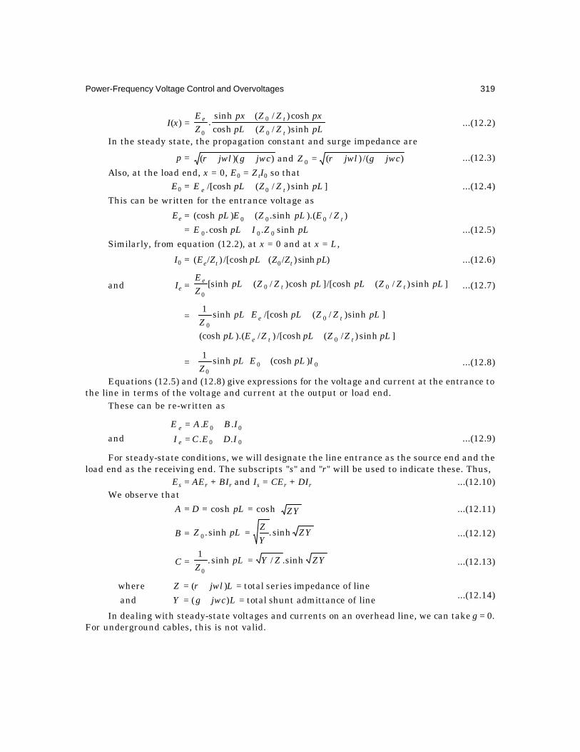
Power-Frequency Voltage Control and Overvoltages 319
I(x) =pLZZpLpxZZpx
ZE
t
te
sinh)/(coshcosh)/(sinh
.0
0
0 ++
...(12.2)
In the steady state, the propagation constant and surge impedance are
p = )/()(and))(( 0 jwcgjwlrZjwcgjwlr ++=++ ...(12.3)
Also, at the load end, x = 0, E0 = ZtI0 so thatE0 = ]sinh)/(/[cosh 0 pLZZpLE te + ...(12.4)
This can be written for the entrance voltage as
Ee = )/).(sinh.()(cosh 000 tZEpLZEpL += pLZIpLE sinh.cosh. 000 + ...(12.5)
Similarly, from equation (12.2), at x = 0 and at x = L,
I0 = )sinh)/(/[cosh)/( 0 pLZZpLZE tte + ...(12.6)
and Ie = ]sinh)/(/[cosh]cosh)/([sinh 000
pLZZpLpLZZpLZE
tte ++ ...(12.7)
= ]sinh)/(/[coshsinh1
00
pLZZpLEpLZ te +
]sinh)/(/[cosh)/).((cosh 0 pLZZpLZEpL tte ++
= 000
)(coshsinh1 IpLEpL
Z+
...(12.8)
Equations (12.5) and (12.8) give expressions for the voltage and current at the entrance tothe line in terms of the voltage and current at the output or load end.
These can be re-written as
and
+=
+=
00
00
..
..
IDECI
IBEAE
e
e
...(12.9)
For steady-state conditions, we will designate the line entrance as the source end and theload end as the receiving end. The subscripts "s" and "r" will be used to indicate these. Thus,
Es = AEr + BIr and Is = CEr + DIr ...(12.10)We observe that
A = D = cosh pL = cosh ZY ...(12.11)
B = ZYYZpLZ sinh.sinh.0 = ...(12.12)
C = ZYZYpLZ
sinh./sinh.1
0
= ...(12.13)
=+==+=
line of admittance shunt total)(and
line of impedance series total)(where
LjwcgYLjwlrZ
...(12.14)
In dealing with steady-state voltages and currents on an overhead line, we can take g = 0.For underground cables, this is not valid.


Power-Frequency Voltage Control and Overvoltages 321
The wavelength λ at 50 Hz is 6000 km based on light velocity of 300,000 km/sec. Therefore,for a line of 100 km, °=λπ 6/2 L . This usually indicates that on an uncompensated line at noload, and when line resistance is negligible, the phase difference between the source voltageand receiving end voltage is 6° for every 100 km of line length at 50 Hz.
12.3 NO-LOAD VOLTAGE CONDITIONS AND CHARGING CURRENTWhen there is no-load at the receiving end, Ir = 0, the control of voltage at line ends posescertain problems due to overvoltage conditions. Unlike dc lines, ac lines have the shunt chargingcurrent flowing through the series inductance of line causing a rise in the output voltage at thereceiving end. This is the well-known "Ferranti Effect." Consider a simple series L-C circuitwith lumped inductance and capacitance, as shown in Figure 12.1 (a) and the phasor diagram ofvoltages and currents in 12.1 (b). By proper voltage division, the source voltage will be
Es = rr ELCwjwcEjwLjwc )1()/1/()/1( 2−=+ ...(12.24)
This shows that Es is less than Er and in phase with it. The voltage drop in the inductivereactance due to the charging current of the capacitor, I = jwC Er, is substracting from the loadvoltage to give the source voltage.
In a distributed-parameter line, neglecting series resistance for understanding thephenomenon, equation (12.5) gives at no load,
Es = )/2cos(.)/cos(.)/(cosh 00 λπ== LEvwLEEvjwL rrr ...(12.25)Since cos 1/ 0 ≤vwL , the source voltage is lower than the receiving-end voltage. Normally,
the source voltage is held constant at the station bus so that the receiving-end bus voltage riseswith line length.
Example 12.1. Calculate the expected p.u. value of load-end voltage for various linelengths from 100 km to 1000 km at no load. Neglect line resistance and assume source-endvoltage to be held constant at 1 p.u.
Solution. The following table shows all values.
L, km 100 200 300 400 500 600 700 800 900 1000°λπ )/2( L 6° 12° 18° 24° 30° 36° 42° 48° 54° 60°
)/2cos( λπL 0.9945 0.978 0.951 0.9135 0.866 0.809 0.743 0.669 0.588 0.5
sr EE / 1.0055 1.022 1.05 1.095 1.155 1.236 1.346 1.494 1.7 2
If we continue this table, we soon find that the ratio Er/Es on a resistanceless line increasesto infinity for a line whose length is equal to one quarter wavelength or 1500 km, and then willdecrease.
Since the standard specifications state the maximum operating voltages for given nominalsystem voltages, some measures must be taken to control the voltage rise at no load at thereceiving end. This requires shunt inductive reactive vars to be provided. If the equipment isconnected only at one end, usually the load end, then a synchronous condenser can be usedoperating in the under-excited condition. However, shunt-compensating reactors either of thefixed type or variable type are used at both ends, and in recent years, static var systems of theswitchable type using high-speed thyristor switches are coming into practice.

322 Extra High Voltage AC Transmission Engineering
Example 12.2. Determine the limiting lengths for uncompensated lines if the voltages atthe two ends must be held at the following sets of values. Neglect resistance and assume no-load condition.
(a) Es = 400 kV, Er = 420 kV,
(b) Es = 380 kV, Er = 420 kV,
(c) Es = 750 kV, Er = 765 kV,(d) Es = 735 kV, Er = 750 kV,
(e) Es = 720 kV, Er = 750 kV,Note that in all cases, Es < Er.Solution. Since Es = )/2cos( λπLEr , the line length is
L = .km),/(cos6
100)]/()[cos2/( 11
rsrs EEEE −− =πλ
For the given data, the line lengths will be(a) 296 km, (b) 420 km, (c) 189 km, (d) 191 km, (e) 271 km.Note that the larger the difference between Es and Er, the longer will be the line length
allowed without shunt reactor compensation.
Charging Current and MVARThe current supplied by the source into the line at no load (Ir = 0) is, from equation (12.10)
Is = rr EpLZ
CE .sinh1
0
= . ...(12.26)
When resistance is neglected,
Z00 = λπ== /2/and/ 0 jvjwpcl .
∴ Is = )/2sin(..)./sin( 0 λπ= LlcjEEvwL
lcj rr ...(12.27)
It leads the receiving-end voltage by 90°. An effective capacitance for the distributed lineconnected across the receiving-end voltage Er and drawing the same current has the value
c0 = ),/2sin(1
00
λπLwZ
Farad. ...(12.28)
The corresponding charging reactive power supplied by the source per phase will be
Q0 = )/2sin(... 0 λπ= LlcEEIE rss . ...(12.29)
If Es and Er are line-to-line voltages in kV, r.m.s., then Q0 will be the 3-phase chargingMVAR. Also,
Q0 = )/2cos(/since),/2tan(..2 λπ=λπ LEELlcE srs ...(12.30)
Note that for a resistanceless line, when L = 2/λ , there is no charging current, andfurthermore, Er = – Es.
Power-Frequency Voltage Control and Overvoltages 323
Example 12.3. For a 400 kV line, l = 1 mH/km and c = 11.1 nF/km, and Es = 400 kV fromthe source, line-line, r.m.s. Calculate the charging MVAR for line lengths varying from 100 kmto 1000 km. Neglect resistance.
Solution. Z00 = cl / = 300 ohms.
L, km 100 200 300 400 500 600 700 800 900 1000
°
1006
tanL
.105 .213 .325 .445 .577 .727 .9 1.11 1.38 1.732
MVARQ ,0 56 113.4 173.3 237.5 308 387.5 480 592 734 924
Q0 /L .56 .567 .578 .594 .616 .646 .686 .74 .816 .924
For normally-encountered distances from 300 km to 600 km, the charging MVAR per 100km is 58 to 65 with an average of 60 MVAR for each 100 km length.
Example 12.4. Repeat example 12.3 for a 750 kV line with surge impedance of Z00 = 250ohms. Take line lengths from 400 km to 1000 km.
Solution. °== )100/6tan(2250.2250/ 0002 LQMWZEs .
L, km 400 500 600 700 800 900 1000Q0, MVAR 1001 1298 1635 2025 2500 3096 3897
For lines between 400 and 1000 km, the charging MVAR is 250 to 390 per 100 km (With anaverage value of 300 MVAR/100 km).
Example 12.5. For the 400-kV and 750-kV lines, calculate the surge-impedance loading,SIL.
Solution. The surge-impedance load is equal to the MVA delivered to a load equal to Z00.This is
SIL = 002/ZEs .
For 400 kV line, SIL = 4002/300 = 533.3 MVA.For 750 kV line, SIL = 7502/250 = 2250 MVA.
Example 12.6. For a 400 kV 400 km line, 50% of the line-charging MVAR is to becompensated by connecting shunt reactors. Calculate the approximate MVAR required in these.
Solution. From example 12.3, the charging MVAR supplied by the source is 237.5 MVAR.For 50% compensation, the shunt reactors have to provide approximately 120 MVAR. In practice,60 MVAR reactors will be connected at each end of line.
More accurate shunt reactor compensation will be calculated in later sections, includingline resistance.
12.4 THE POWER CIRCLE DIAGRAM AND ITS USEEquation (12.10) can also be written for Er and Ir in terms of Es and Is as follows, with AD – BC= 1, and A = D:
r
r
IE
=
−
−=
−
s
s
s
s
IE
DCBA
IE
DCBA
,
,
,
,1
...(12.31)

324 Extra High Voltage AC Transmission Engineering
Also, Ir = (Es – AEr)/B ...(12.32)All these quantities are complex numbers. The receiving-end power is
Wr =***** /)( BEAEEIEjQrP rsrrrr −==+ ...(12.33)
If we consider Er as reference giving °∠= 0rr EE , then the sending-end voltage Es = |Es| δ∠ ,where the angle δ is called the power angle. Also let A = |A| aθ∠ and B = |B| bθ∠ . Then
Wr = )||.|(||| ars
brrr AEE
BE
jQP θ−∠−δ−∠θ∠
=+
= )(||
||)(
|||| 2
abr
bsr
BAE
BEE
θ−θ∠−δ−θ∠ ...(12.34)
Separating the real and j-parts, there result
Pr = )cos(||
||)cos(
|||| 2
abr
bsr
BAE
BEE
θ−θ−δ−θ ...(12.35)
and Qr = )sin(||
||)sin(
|||| 2
abr
bsr
BAE
BEE
θ−θ−δ−θ ...(12.36)
These can be re-written as
δ−θ=θ−θ+
δ−θ=θ−θ+
)sin(||
||)sin(
||||
)cos(||
||)cos(
||||
2
2
bsr
abr
r
bsr
abr
r
BEE
BAE
Q
BEE
BAE
P
...(12.37)
Then, eliminating δ by squaring and adding the two equations, we obtain the locus of Pr
against Qr to be a circle with given values of A and B, and for assumed values of Er and |Es| asfollows:
2222
)sin(||
||)cos(
||
||
θ−θ++
θ−θ+ abr
rabr
rB
AEQ
B
AEP
=
2
||
||
BEE sr
...(12.38)
The coordinates of the centre of the receiving-end power-circle diagram are
θ−θ−=
θ−θ−=
MVAR.),sin(||
||
and,MW),cos(||
||
2
2
abr
c
abr
c
B
AEy
B
AEx
...(12.39)
The radius of the circle isR = MVA|,|/||. BEE sr . ...(12.40)

Power-Frequency Voltage Control and Overvoltages 325
Figure 12.2 shows the receiving-end circle diagram. If the receiving-end voltage is heldconstant, as is usually dictated by the load, the centre of the circle is fixed, but the radius willdepend on the value of the sending-end voltage, Es. Therefore, for a chosen variation in |Es|,a system of circles with centre at C and proper radius given by equation (12.40) can be drawn.The power-circle diagram and the geometrical relations resulting from it are extremely usefulto a design engineer and an operating engineer to determine the status of power flow, reactivepower flow, compensation requirements for voltage control and many properties concerningthe system. These will be illustrated through typical examples.
Referring to Figure 12.2, the angle ∠ OCPm = )( ab θ−θ and from equations (12.35) and(12.36), when Pr = 0, that is when the circle intersects the vertical axis at O'.
R cos )( 0δ−θb = |xc|, giving ∠ O'CPm = (θb – δ0) ...(12.41)
Fig. 12.2 Receiving-end circle diagram for calculating reactive compensation forvoltage control at buses.
It is therefore a simple matter to find the angle 0δ at no-load. For any other load, the loadline is drawn with given MW and MVAR along the horizontal and vertical axes shown as PL andQL. Let the circle intersect the load line at O". Then, δ−θ=∠ bmO"CP , from equation (12.35).Because of geometrical construction using instruments, there will be slight inherent errorinvolved in the results but will serve engineering purposes. However, with the aid of DigitalComputers, great accuracy can be achieved from the properties relating to the circle diagram.
Maximum PowerFor a given set of Er, Es, A and B, the maximum power that can be transmitted, Pm, is
Pmax = )(cos||
||||
||||
2
abrsr
c BAE
BEE
xR θ−θ−=− ...(12.42)
and the corresponding power angle is
maxδ = mb O'CP∠−θ ...(12.43)
Cx, y( )c c
θb a – θ
θb – δ
δ
E AB
r2 | || |
Es
Pm
R1
PL
QL
Pr
|Es1| < |E |s2
O
O'
O"Load line
Er
E EB
r s | || |
2R2 =
Qr

326 Extra High Voltage AC Transmission Engineering
For the case when resistance is neglected,
A = cosh pL = cos wL/v0, giving 0=θa , and
B = °=θ= 90giving,/sin.//sinh./ 00 bvwLcljvjwLcl .
∴ maxP = )/sin'/(||||/|| 000 vwLZEEBEE srsr = ...(12.44)From (12.35) and (12.36), with θa = 0 and θb = 90°,
||/sin.|| BEEP srr δ= , which is maximum when °=δ 90 and so Pmax = Er|Es|/|B|. Weobserve from equation (12.44) that |B| = Z00. sin wL/v0. Normally, resistances should not beneglected since the line losses for a given system status are one of the governing quantities insystem design and compensation calculations.
Example 12.7. The following details are given for a 750-kV 3-phase line: Resistance r =0.014 ohm/km, inductance l = 0.866 mH/km, reactance x = 0.272 ohm/km at 50 Hz, c = 12.82nF/km giving a susceptance of y = 4.0275 × 10⁻⁶ mho/km, velocity v0 = 3 × 10⁸ m/s = 3 × 10⁵ km/sec, line length = 500 km. Calculate items (a) and (b) below, and work parts (c) and (d). Giveproper units for all quantities.
(a) clZjwcLYjwlrLZ /,),( 00 ==+= .
(b) The generalized constants A, B, C, and D, in both polar and rectangular forms.
(c) For Er = 750 kV and |Es| = 0.98 Er, determine the coordinates of the centre of thereceiving-end power-circle diagram and the radius.
(d) Find the power angle δ for transmitting a load of 2000 MW at 750 kV at the receiving-end at unity power factor.
Solution.
(a) Z = 500(0.014 + j0.272) = 7 + j136 = 136.2∠ 87°, ohms.Y = j500 × 4.0275 × 10–6 = j 2.014 × 10–3 = 2.014 × 10⁻³ ∠ 90°, mho.
Z00 = 31082.12/866.0 × = 260 ohms.
(b) ZY = (136.2 × 2.014 × 10–3)1/2∠ 88.5° = 0.5237 ∠ 88.5°
= 0.0137 + j0.5235. (0.5235 radian = 30°)
YZ / = (136.2/2.014 × 10–3)1/2∠ –1.5°
= 260∠ –1.5° = 259.9 – j6.8 ohms.
∴ A = D = cosh ZY = cosh 0.0137. cos 0.5235 + jsinh 0.0137. sin 0.5235
= 0.86625 + j0.00685 = 0.8663 ∠ 0.45°[At no load, without compensation, for Er = 750 kV, Es = AVr = 650 kV, line-line].
C = ZYZY sinh/ = sinh (0.0137 + j 0.5235)/260 ∠ –1.5°
= (sinh 0.0137. cos 0.5235 + jcosh 0.0137. sin 0.5235)/260 °−∠ 5.1
= 0.50024 ∠ 88.64°/260 ∠ –1.5° = 1.924 × 10⁻³ ∠ 90.14°.= (–0.0047 + j1.923994) 10–3 mho.
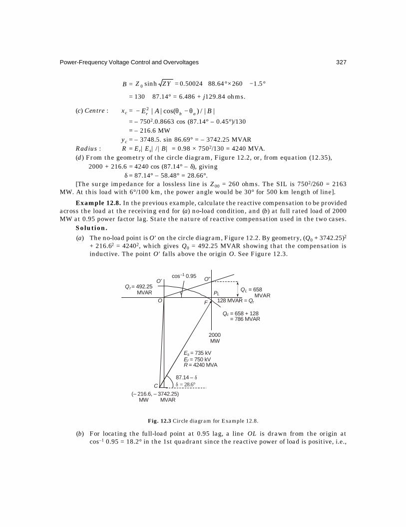
Power-Frequency Voltage Control and Overvoltages 327
B = °−∠×°∠= 5.126064.8850024.0sinh0 ZYZ
= 130∠ 87.14° = 6.486 + j129.84 ohms.
(c) Centre : xc = ||/)cos(||2 BAE abr θ−θ−= – 7502.0.8663 cos (87.14° – 0.45°)/130= – 216.6 MW
yc = – 3748.5. sin 86.69° = – 3742.25 MVARRadius : R = Er|Es|/|B| = 0.98 × 7502/130 = 4240 MVA.(d) From the geometry of the circle diagram, Figure 12.2, or, from equation (12.35),
2000 + 216.6 = 4240 cos (87.14° – δ), givingδ = 87.14° – 58.48° = 28.66°.
[The surge impedance for a lossless line is Z00 = 260 ohms. The SIL is 7502/260 = 2163MW. At this load with 6°/100 km, the power angle would be 30° for 500 km length of line].
Example 12.8. In the previous example, calculate the reactive compensation to be providedacross the load at the receiving end for (a) no-load condition, and (b) at full rated load of 2000MW at 0.95 power factor lag. State the nature of reactive compensation used in the two cases.
Solution.
(a) The no-load point is O' on the circle diagram, Figure 12.2. By geometry, (Q0 + 3742.25)2
+ 216.62 = 42402, which gives Q0 = 492.25 MVAR showing that the compensation isinductive. The point O' falls above the origin O. See Figure 12.3.
Fig. 12.3 Circle diagram for Example 12.8.
(b) For locating the full-load point at 0.95 lag, a line OL is drawn from the origin atcos–1 0.95 = 18.2° in the 1st quadrant since the reactive power of load is positive, i.e.,
(– 216.6, – 3742.25) MW MVAR
C87.14 – δδ = 28.6°
EER
sr
= 735 kV = 750 kV = 4240 MVA
Qc = 658 + 128 = 786 MVAR
QL = 658 MVAR
2000MW
128 MVAR = Qr
Qr = 492.25 MVAR
O'
O F
PL
O"cos 0.95–1

328 Extra High Voltage AC Transmission Engineering
inductive, equal to QL = 2000 tan 18.2° = 658 MVAR. From the circle diagram,22 |)|()|(| cLLc xPFPy ++− = R2
or, (3742.25 – PLF)2 + (2000 + 216.6)2 = 42402
giving PLF = 128 MVAR, capacitive, since the point F was taken below the horizontal orpower axis. This is the total reactive power required at the receiving end across the load for thegiven voltage and load conditions. To this must be added 658 MVAR of the load itself in order toobtain the rating of the compensating equipment, which not only has to override the 658 MVARinductive of the load but also provide 128 MVAR capacitive. Therefore, the rating of thecompensating equipment will be 658 + 128 = 786 MVAR, capacitive. From equation (12.35), thepower angle is δ = 28.66°, which can also be obtained from equation (12.36) by using Qr= – 128MVAR.
From the above example, it may be observed that at no load inductive compensation isnecessary amounting to 492.25 MVAR and at full load the compensation required is capacitiveamounting to 786 MVAR. The ratio of inductive to capacitive MVAR's is 492.25/786 = 0.626.
Example 12.9. If in the previous example, the sending-end voltage is raised to 750 kV,the same as Er, calculate the compensation to be provided (a) at no load, (b) at full load, and(c) the power angle δ in the two cases.
Solution. Since Er, A, and B are the same, the coordinates of the centre of the receiving-end circle diagram stay the same at (– 216.6 MW, – 3742.25 MVAR). But the new radius is R =7502/130 = 4327 MVA.
(a) At no load: (Q0 + 3742.25)2 + 216.62 = 43272 giving
Q0 = 580 MVAR, inductive.
(b) At full load: (3742.25 – PLF)2 + 2216.62 = 43272 givingPLF = 26 MVAR, capacitive. Therefore, adding 658 MVAR of the load, the compensating
equipment must provide a reactive power of 684 MVAR, capacitive. Since the load can varyfrom no-load to full-load, this will be in the nature of switched capacitors. The ratio of inductiveMVAR to capacitive MVAR = 580/684 = 0.848. Notice that power can flow in an ac system froma point at any voltage to another of equal voltage or even at higher voltage, provided the propertype and sufficient amount of reactive compensation is utilized. This is impossible in a dcsystem.
(c) The power angles are °=δ 00 and °=δ 5.28l .
12.5 VOLTAGE CONTROL USING SYNCHRONOUS CONDENSERSFrom the generalized constants (A, B, C, D) of a given input port and output port, the power-circle diagram or the corresponding geometrical relations can be utilized for deciding the propercompensating MVAR's to be provided at the receiving end when a set of magnitudes for Er andEs at the two ends of the line are specified. When the load has a lagging power factor or even aunity power factor, generally the control of voltage is achieved by providing leading powerfactor or capacitive compensation at the receiving end. This can take the form of switchedcapacitors, usually connected to the low-voltage tertiary of the substation transformer at theload end. At no-load, usually inductive reactive compensation is required if the sending-endvoltage is to be raised to stay within the standard specifications. This is provided by either theswitched type (regulated) or constant type (unregulated).

Power-Frequency Voltage Control and Overvoltages 329
The synchronous condenser provides both types of MVAR's, lagging or leading, that isinductive or capacitive. The synchronous motor runs without a shaft load and is enclosed in anexplosion-proof casing which is filled with hydrogen at above atmospheric pressure in order tominimize rotational losses, and to ensure that any leakage of gas will be from the inside toexternal air, thus preventing an explosive mixture to be formed. The reactive powers generatedby the motor are controlled by varying the dc field excitation of the rotor, under-excitationproviding inductive MVAR's and over-excitation yielding capacitive MVAR's. Because oflimitations imposed on excitation, the synchronous phase modifier can provide only 60 to 70%of its rated capacity at lagging power factor (under-excited condition) and full rated leadingreactive power (over-excited condition).
The design of the rating of the synchronous phase modifier (or condenser for short) andthe voltage conditions are illustrated below. The general equation satisfied by the real andreactive powers at the load end at any point on the circle is
(Pr + |xc|)2 + (Qr + |yc|)2 = R2 ...(12.45)At no load, the point O' in Figure 12.2, obviously Pr = 0. The reactive power is
Q0 = ||22cc yxR −− ...(12.46)
At full load, point O" in Figure 12.2 or 12.3,(PL + |xc|)2 + (|yc| – Qr)2 = R2 ...(12.47)
∴ The total reactive power required at the receiving end is
Qr = |yc|22
|)|( cL xPR +−− ..(12.48)
The capacitive MVAR required in the synchronous condenser is then
Qc =22 |)|(|| cLcLrL xPRyQQQ +−−+=+ ...(12.49)
If we use the relation )1(,0 <= mmQQ c , then the equation to be satisfied by the radius of
the circle, which is the only quantity involving the sending-end voltage Es will be, when valuesfor Er, A, B, PL, QL are specified,
2222 |)|( ccL xRxPRm −++− = Lc mQym ++ ||)1( ...(12.50)
When all quantities except R are specified, equation (12.50) will yield the value ofBEER sr |/||= |, from which the sending-end voltage is determined. This is shown by the
following example.
Example 12.10. For Example 12.9, taking Er = 750 kV and m = 0.7 for the synchronouscondenser, determine (a) the sending-end voltage, and (b) the proper rating of the synchronouscondenser.
Solution. The data given are
Er = 750, A = 0.8663 ∠ 0.45°, B = 130 ∠ 87.14°, xc = – 216.6,yc = – 3742.25, PL = 2000 MW, QL = 658 MVAR inductive, and m = 0.7.
(a) Solving equation (12.50) for R there resultsR = 4272 = 750 × Es/130.
∴ The sending-end voltage has the magnitudeEs = 4272 × 130/750 = 740 kV, line-line.

330 Extra High Voltage AC Transmission Engineering
(b) The synchronous-condenser rating is Qc = QL + Qr, from equation (12.49).
Qr = 3742.25 – 22 )6.2162000(4272 +− , from equation (12.48)
= 90 MVAR, capacitive at full load.∴ Qc = 90 + 658 = 748 MVAR, over-excited.As a check, the under-excited reactive power required at no load is given by equation
(12.46) as
Q0 = 22 6.2164272 − – 3742.25 = 519 MVAR, inductive.
The ratio of under-excited to over-excited MVAR's isQ0/Qc = 519/748 = 0.694 ≈ 0.7.
The rating of the synchronous condenser would be about 750 MVAR when deliveringcapacitive reactive power at over-excited condition of operation.
In order to use the circle diagram, a series of circles should be drawn with several chosenvalues of magnitude of Es and picking values of compensation required at no load and full load.The value yielding a ratio of m = Q0/Qc = 0.7 will be the magnitude of the sending-end voltage, Es.
12.6 CASCADE CONNECTION OF COMPONENTS–SHUNT AND SERIESCOMPENSATION
In the previous sections, the (A, B, C, D) constants of only the line were considered. It becomesevident that through the example of the 750 kV line parameters, it is impossible to control thevoltages within limits specified by IS and IEC by providing compensation at one end only bysynchronous condensers, or by switched capacitors if the voltages are to vary over wider limitsthan discussed. In practice, shunt-compensating reactors are provided for no-load conditionswhich are controlled by the line-charging current entirely, and by switched capacitors for full-load conditions when the load has a lagging power factor.
Generalized EquationsFor no-load conditions, Zt = ∞ , and the equations for sending-end and receiving-end voltagesare, Figure 12.4,
Er = Es/[cosh pL + (Z0/Zsh)sinh pL] ...(12.51)For simplicity, let r = 0. Then,
p = ,,/,/2/ 0000 shsh jXZclZZjvjw ===λπ=
so that Es/Er = ./2sin)/(/2cos 00 λπ+λπ LXZL sh ...(12.52)
When the ratio Es/Er is given for a system, the value of Xsh is easily determined. Inparticular, when Es = Er,
Zsh = )/2cot/2cosec/(00 λπ−λπ LLZ . ...(12.53)
Example 12.11. For the 750-kV line of previous examples, L = 500 km, λ = 6000 km at 50Hz and Z00 = 260 ohms. Assuming Es = Er = 750 kV, calculate the reactance and 3-phase MVARrequired at load end in the shunt-compensating reactor. Neglect line resistance.
Solution. 2πL/λ = 30° at 6° per 100 km of length of line.∴ Xsh = 260/(cosec 30° – cot 30°) = 3.73 × 260 = 970 ohms.
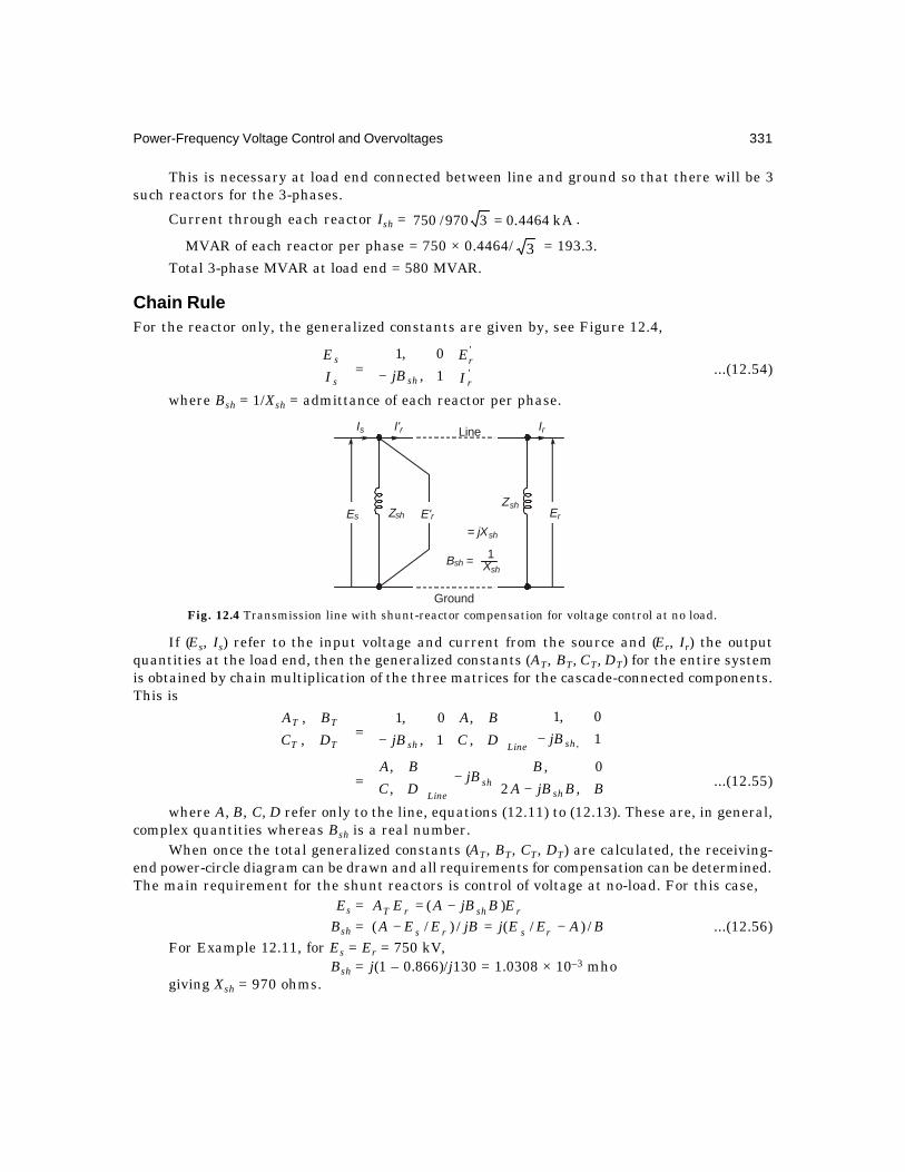
Power-Frequency Voltage Control and Overvoltages 331
This is necessary at load end connected between line and ground so that there will be 3such reactors for the 3-phases.
Current through each reactor Ish = kA4464.03970/750 = .
∴ MVAR of each reactor per phase = 750 × 0.4464/ 3 = 193.3.
Total 3-phase MVAR at load end = 580 MVAR.
Chain RuleFor the reactor only, the generalized constants are given by, see Figure 12.4,
s
s
IE
=
− '
r
'r
sh I
EjB 1,
0,1...(12.54)
where Bsh = 1/Xsh = admittance of each reactor per phase.
Fig. 12.4 Transmission line with shunt-reactor compensation for voltage control at no load.
If (Es, Is) refer to the input voltage and current from the source and (Er, Ir) the outputquantities at the load end, then the generalized constants (AT, BT, CT, DT) for the entire systemis obtained by chain multiplication of the three matrices for the cascade-connected components.This is
TT
TT
DCBA
,
, =
−
− 1
0,1
,
,
1,
0,1
,shLinesh jBDCBA
jB
=
−
−
BBjBA
BjB
DCBA
shsh
Line ,2
0,
,
,...(12.55)
where A, B, C, D refer only to the line, equations (12.11) to (12.13). These are, in general,complex quantities whereas Bsh is a real number.
When once the total generalized constants (AT, BT, CT, DT) are calculated, the receiving-end power-circle diagram can be drawn and all requirements for compensation can be determined.The main requirement for the shunt reactors is control of voltage at no-load. For this case,
Es = rshrT EBjBAEA )( −=∴ Bsh = BAEEjjBEEA rsrs /)/(/)/( −=− ...(12.56)For Example 12.11, for Es = Er = 750 kV,
Bsh = j(1 – 0.866)/j130 = 1.0308 × 10⁻³ mhogiving Xsh = 970 ohms.
ErEs E'rZshZsh
= jXsh
1Xsh
Bsh =
Is I'r Line
Ground
Ir
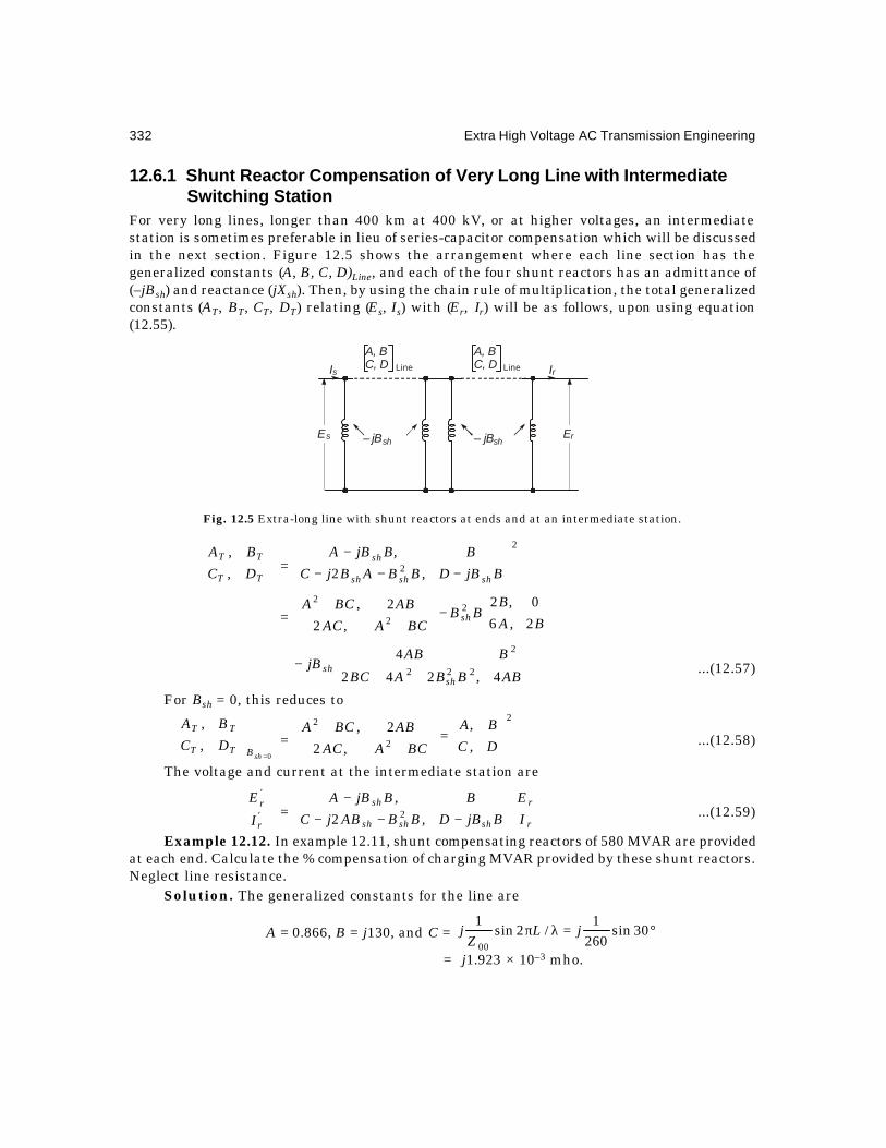
332 Extra High Voltage AC Transmission Engineering
12.6.1 Shunt Reactor Compensation of Very Long Line with Intermediate Switching Station
For very long lines, longer than 400 km at 400 kV, or at higher voltages, an intermediatestation is sometimes preferable in lieu of series-capacitor compensation which will be discussedin the next section. Figure 12.5 shows the arrangement where each line section has thegeneralized constants (A, B, C, D)Line, and each of the four shunt reactors has an admittance of(–jBsh) and reactance (jXsh). Then, by using the chain rule of multiplication, the total generalizedconstants (AT, BT, CT, DT) relating (Es, Is) with (Er, Ir) will be as follows, upon using equation(12.55).
Fig. 12.5 Extra-long line with shunt reactors at ends and at an intermediate station.
TT
TT
DCBA
,
, =
2
2 ,2
,
−−−
−BjBDBBABjC
BBjBA
shshsh
sh
=
−
++
BAB
BBBCAAC
ABBCAsh 2,6
0,2
,2
2, 22
2
++−
ABBBABC
BABjB
shsh
4,242
4222
2
...(12.57)
For Bsh = 0, this reduces to
0,
,
=
shBTT
TT
DCBA
=
2
2
2
,
,
,2
2,
=
++
DCBA
BCAACABBCA
...(12.58)
The voltage and current at the intermediate station are
'r
'r
I
E =
−−−
−
r
r
shshsh
sh
IE
BjBDBBABjCBBjBA
,2
,2 ...(12.59)
Example 12.12. In example 12.11, shunt compensating reactors of 580 MVAR are providedat each end. Calculate the % compensation of charging MVAR provided by these shunt reactors.Neglect line resistance.
Solution. The generalized constants for the line are
A = 0.866, B = j130, and C = °=λπ 30sin2601
/2sin1
00
jLZ
j
= j1.923 × 10–3 mho.
Es
Is Ir
Er– jBsh – jBsh
A, BC, D Line
A, BC, D Line

Power-Frequency Voltage Control and Overvoltages 333
∴ Charging MVAR of line without shunt reactors is
Q0 =2sCE = j1.923 × 10–3 × 7502 = 1082 MVAR.
With shunt reactors, with Bsh = 1.0308 × 10⁻³ mho, from equation (12.55),
CT = 010)138.07854.1923.1(2 32 ≈−−=−− −jBBBAjC shsh .
∴ % compensation is total or 100%.
Example 12.13. For the examples 12.11 and 12.12, instead of 580 MVAR, allow 60% shuntreactor compensation to maintain Es = 750 kV. Calculate the MVAR of the shunt reactors ateach end, and the voltage at the receiving end at no-load.
Solution. % compensation = 100 (C – CT)/C, givingCT = (1 – 0.6) C = 0.4 C = j0.4 × 1.923 × 10–3 mho
= j0.7692 × 10–3 mho.
But CT = ,2 2 BBBAjC shsh −−
or j0.7692 × 10–3 = j1.923 × 10–3 – j2 × 0.866 × Bsh – j130 2shB .
Solving the quadratic equation for Bsh resultsBsh = 0.6358 × 10⁻³ mho.
∴ 3-phase MVAR of each shunt-reactor bank at 750 kV will be
Qsh =2sshEB = 0.6358 × 10–3 × 7502 = 358 MVAR.
[Note that this may be approximately 60% of 580 MVAR which was required for 100%compensation.]
With these reactors connected, the receiving-end voltage will not be 750 kV. It is calculatedas follows:
AT = A – jBsh B = 0.866 + 0.6358 × 10–3 × 130 = 0.9486.∴ Er = Es/AT = 790.6 kV.The compensation is a bit low since the bus voltage at the receiving end is higher than 765
kV, which is specified by IS and IEC. If Er is to be held at 765 kV, then Es must be lowered. SinceAT = 0.9486, Es = 0.9486 × 765 = 726 kV. Then, the shunt-reactor rating will be
Qshs = 7262 × 0.6358 × 10–3 = 335 MVAR at the sending end,and Qshr = 7652 × 0.6358 × 10–3 = 372 MVAR at the receiving end.
A compromise of 350 MVAR would be selected and the voltages at the two ends adjusted.
Example 12.14. A 400-kV line is 800 km long. Its inductance and capacitance per km arel = 1 mH/km and c = 11.1 nF/km (Z00 = 300 ohms). The voltages at the two ends are to be heldat 400 kV at no load. Neglect resistance. Calculate
(a) MVAR of shunt-reactors to be provided at the two ends and at an intermediate stationmidway with all four reactors having equal reactance.
(b) The A, B, C, D constants for the entire line with the shunt reactors connected.
(c) The voltage at the intermediate station. (Use 6°/100 km).Solution. Refer to Figure 12.5 and equations (12.57) and (12.59). For one 400-km section:(a) A = D = cos 24° = 0.9135, B = j300 sin 24° = j122 ohm and
C = (sin 24°)/300 = j1.356 × 10–3 mho.
334 Extra High Voltage AC Transmission Engineering
The total AT from end to end for 800 km is
AT = shsh ABBjBBBCA 42 222 −−+
= 2768,298.445669.0 shsh BB ++ .
But since Es = Er, the value of AT = 1.
By using this value of AT and solving for Bsh yields Bsh = 0.709 × 10⁻³ mho. The MVAR ofeach of the reactors at the two ends will be
Qe = 4002 × 0.709 × 10–3 = 113.4 MVAR, 3-phase unit.(b) The A, B, C, D constants for the entire line are found as follows:From equation (12.55), for each 400-km section,
BjBA sh− = 0.9135 + 0.709 × 10–3 × 122 = 1
)2( BjBAjBC shsh −− = )122.709.0827.1(10709.010356.1 33 ×+××−× −− jj
= 0.
∴
TT
TT
DCBA
,
, =
=
1,0
244,1
1,0
122,12 jj
(c) At the intermediate station, kV400.1 == s'r EE .
12.6.2 Series-Capacitor Compensation at Line CentreIn order to increase the power-handling capacity of a line, the magnitude of B must be reduced,as shown in equations (12.35) and (12.44). In normal practice, °≈θ 90b and 0≈θa for very low
series line resistance. Therefore, P = ErEs.sin B/δ . We also observe that the value of B is verynearly equal to the series inductive reactance of the line so that by employing capacitors connectedin series with the line, the power-handling capacity of a line can be increased for chosen valuesof Es, Er and δ . All these three quantities are limited from considerations of highest equipmentvoltages and stability limits. Usually, the series capacitor is located at the line centre when onecapacitor only is used, or at the one-third points if two installations are used. On a very longline with intermediate station, the series capacitor can be located here. In this section we willonly consider the generalized constants when a series capacitor is located at the line centrewithout intermediate shunt-reactor compensation. Thus, the system considered consists ofequal shunt reactor admittances Bsh at the two ends and a capacitor with reactance xc at theline centre, as shown in Figure 12.7.
For each half of the line section of length L/2,
A' = ,4/sinh,4/cosh 0 ZYZB'ZYD' ==
C' = 4/sinh1
0
ZYZ ...(12.60)
where Z and Y refer to the total line of length L. The surge impedance is not altered eventhough the line length is halved.

Power-Frequency Voltage Control and Overvoltages 335
For the series capacitor, Figure 12.6(b), the voltages and currents on the two sides arerelated by
Fig. 12.6 Transmission line with series-capacitor compensation in middle of line.
's
's
I
E =
−'r
'rc
I
Ejx1,0
,1...(12.61)
Thus, for the two half-sections of line with the capacitor separating them, the totalgeneralized constants will be, by the chain rule of multiplication, (Figure 12.6a),
TT
TT
DCBA
,
, = ×
−
1,0
,14/cosh,4/sinh
14/sinh,4/cosh
0
0cjx
ZYZYZ
ZYZZY
=
ZYZYZ
ZYZZY
ZYZYZ
ZYZZY
cosh,sinh1
sinh,cosh
4/cosh,4/sinh1
4/sinh,4/cosh
0
0
0
0
−
+−
ZYZYZ
ZYZZY
Zx
j c
sinh),1(cosh1
)1(cosh,sinh
20
0
0...(12.62)
=
−
+−
pLpL
Z
pLZpL
Zx
jDCBA c
sinh),1(cosh1
)1(cosh,sinh
2,
,
0
0
0Line...(12.63)
With no series capacitor, xc = 0, equation (12.63) reduces to the generalized constants ofthe line.
Shunt Reactors at Both Ends and Series Capacitor in Middle of LineIf shunt-compensating reactors of admittance Bsh are located at both ends of line, the totalgeneralized constants with series capacitor located in the line centre can be obtained in theusual way by using the chain rule, from Figure 12.7. It is left to the reader to verify the result.
Es Er E's E'r
Is – jXc – jXcIr
I's I'rL/2 L/2
( )a ( )b

336 Extra High Voltage AC Transmission Engineering
Fig. 12.7 Transmission line with series capacitor in middle and shunt reactors at ends.
TT
TT
DCBA
,
, =
−−
BBjBA
BjB
DC
BA
shsh
,2
0,
,
,
Line
−
+− pLpL
Z
pLZpL
Z
xj c
sinh),1(cosh1
)1(cosh,sinh
0
0
0
++−
+− 1cosh),1(coshsinh
20,1cosh
20
pLpLjBpLZ
pLBxsh
shc...(12.64)
W e must point out that all quantities except xc and Bsh are complex numbers with amagnitude and phase angle.
If shunt reactors are not used, Bsh = 0, then equation (12.64) reduces to (12.63). If no seriescapacitor is used, equation (12.55) results.
The value of capacitance is chosen such that its reactance amounts to a chosen percentageof the series inductive reactance of the line. For example, if 50% series capacitance is to beprovided for a 800 km 400 kV line having a series inductive reactance of j 244 ohms, thecapacitive reactance is – j 122 ohms. The required capacitance will be C = 1/wxc = 26 µF at 50Hz. The power-handling capacity of a line with 50% series compensation will increase to doublethat without series capacitor.
While the power-handling capacity can be increased, series capacitor compensation resultsin certain harmful properties in the system, chief among them are:
(a) Increased short-circuit current. Note that for a short-circuit beyond the capacitorlocation, the reactance is very low. At the load-side terminal of the capacitor, a short-circuit will result in infinite current for 50% compensation.
(b) Sub-harmonic or sub-synchronous resonance conditions during load changes and short-circuits. This has resulted in unexpected failures to long shafts used in steam-turbine-driven alternators and exciters when one or more of the resulting sub-harmoniccurrents due to series compensation can produce shaft torques that correspond toone of the several resonance frequencies of the shaft, called torsional modes ofoscillation or critical speeds. This aspect will be discussed in some detail and countermeasures used against possible failure will be described in the next section.
Es Er
Is
– jXc
Ir
L/2
– jBsh
L/2
– jBsh

Power-Frequency Voltage Control and Overvoltages 337
12.7 SUB-SYNCHRONOUS RESONANCE IN SERIES-CAPACITORCOMPENSATED LINES
12.7.1 Natural Frequency and Short-Circuit CurrentWith series compensation used, the power-handling capacity of a single circuit is approximately
P = ssr XEE /sin. δ ...(12.65)
where sX = )1( mXXX LcL −=− ...(12.66)with m = Xc/XL = degree of compensation, and the reactances are at power frequency f0.
The approximation occurs because we have considered the series inductive reactance XL to belumped. At any other frequency f,
)( fX L = LfLπ2 = total inductive series reactance of line
and )( fX c = fCπ2/1 = series capacitive reactance of capacitor.
∴ The resonance frequency occurs when )()( eceL fXfX = giving
LeLfπ2 = Cfeπ2/1 ...(12.67)We can introduce the power frequency f0 by re-writing equation (12.67)
as )/)(2( 00 ffLf eLπ = )]/.(2/[1 00 ffCf eπ at resonance.
Consequently,2
0 )/( ffe = mXXCfLf LcL ==ππ /)2).(2/(1 00 . ...(12.68)
Thus, the electrical resonance frequency is mffe 0= ...(12.69)The reduction of series reactance also reflects as decrease in effective length to
LmLe )1( −= .For f0 = 50 Hz and 60 Hz, and for various degrees of series compensation, the following
table gives the resonant frequencies and effective length which are also plotted in Figure 12.8.
m = Lc XX / 0.1 0.2 0.3 0.4 0.5 0.6 0.7 0.8 0.9 1.0% compensation 10 20 30 40 50 60 70 80 90 100
0/ffe 0.3162 0.447 0.548 0.632 0.707 0.775 0.837 0.894 0.949 1fe for 50Hz 15.8 22.4 27.4 31.6 35.36 38.7 41.8 44.7 47.4 50fe for 60Hz 18.97 26.8 32.9 37.95 42.4 46.5 50.2 53.7 56.9 60Le /L = 1 – m 0.9 0.8 0.7 0.6 0.5 0.4 0.3 0.2 0.1 0
Fig. 12.8 Variation of resonance frequency fe and effective length Le of line with degree of seriescompensation (XC/XL).
1.0
0.8
0.6
0.4
0.2
00 .2 .4 .6 .8 1.0
L L1/
f fe/ 0
m X X= /c L

338 Extra High Voltage AC Transmission Engineering
For a single line with series compensation between 40% and 70%, the line can resonate atfrequencies between 63.25% and 83.7% of the power frequencies. Any disturbance in the linegiving rise to currents at these frequencies will increase the voltage across the series capacitorand therefore the line drop to extremely high values which are limited only by the line resistance.The voltage across the capacitor during normal operation is IXV cc = , where I = currentflowing in line.
Example 12.15. A 50-Hz 750 kV line with l = 0.866 mH/km is 500 km long. It is providedwith 50% series compensation connected in the middle of line. The power delivered at 750 kVis 2000 MW 3-phase per circuit at unity power factor. Neglect shunt capacitance and lineresistance and assume the line inductance to be lumped. Calculate
(a) the reactance and capacitance of series capacitor,
(b) the voltage drop across it at full load,
(c) the current flowing through it and the voltage across it during a sustained short-circuit occurring(i) on the source-side terminal of the capacitor,
(ii) on the load-side terminal of the capacitor, and
(iii) across the load.
(d) the same as in (c) without the series capacitor.
Fig. 12.9. Illustrating dangers of increased short-circuit currents with series-capacitor compensationfor faults at various important locations.
Assume that no other generating area is supplying the load. See Figure 12.9.Solution. Total series reactance of 250 km of line at 50 Hz is
314 × 0.866 × 10–3 × 250 = 68 ohms.(a) For 50% compensation, Xc = 68 ohms and C = 46.8 µF.
(b) At full load, I = 2000/750 3 = 1.54 kA = 1540 Amps.
∴ Voltage across capacitor Vc = 68 × 1.54 = 104.7 kV.
(c) (i) For a short-circuit to ground occurring at point A, the capacitor will dischargethrough the fault and its voltage will become zero. There will be an oscillatorystage consisting of a circuit with the capacitor, line reactance of j68 ohms and theload impedance.
7503
A B C
Load
j68 – j68 j68
Source

Power-Frequency Voltage Control and Overvoltages 339
(ii) For a short-circuit at point B, we observe that the steady-state component ofcurrent is infinity and dangerously high voltage will exist across the capacitor.Under such a condition, arrangements must be made to bypass the capacitor bya gap that will flashover at a preset overvoltage value. This is normally set at 2.2p.u. where 1 p.u. voltage = voltage across capacitor during normal operationwhich was calculated as 104.7 kV. These protective schemes will be describedlater on.
(iii) When a short-circuit occurs at point C, the sustained r.m.s. value of current is
Isc = 750/68 3 = 6.368 kA = 4.135 × full-load current.
The voltage across the capacitor will be Vc = kV4333/750 = . This is the lowestvalue of voltage across the capacitor for a short-circuit occurring at any place on theline between points B and C.
(d) Without the series capacitor, the currents during short circuit at points A or B and Cwill be 6.368 kA and 3.184 kA respectively. Consequently, using a series capacitorhas increased the short-circuit level of the system.
Protective Schemes for Series CapacitorSome of the methods used in practice for protecting series capacitors from damage due toovervoltages and overcurrents are described below and shown in Figure 12.10. In some schemes,the capacitor banks are protected by a sparkover gap that will either short-circuit the capacitoror otherwise use a voltage-limiting surge arrester of the gap-SiC type or gapless ZnO type.When the short-circuit in the system is cleared, the capacitor is re-inserted in order to preservethe stability of the system. The re-insertion transient can be very high and cause gap flashover.This is prevented by either parallel resistor or SiC and ZnO arresters. The sparkover voltage ofthe gap G is between 2.2 and 3.5 p.u. of normal capacitor voltage at full rated current.
Fig. 12.10 Protective schemes for series capacitors during abnormal conditions.
Line Line
Gap
Arrester
S L
C
SiC
Line Line
Arrester
S L
C
ZnO
Line LineC
Arrester
G
VoltageDivider
Power Gap
Bypass Switch

340 Extra High Voltage AC Transmission Engineering
12.7.2 Sub-Synchronous Resonance Problem and Counter MeasuresAs pointed out before, electrical resonance frequencies lower than synchronous frequency f0exist when series-capacitor compensation is used. The frequency f0 corresponds to the steady-state speed of the rotor in large power stations. With steam-turbine-driven generating units(designated T.G. units), the shaft or shaft portions connecting the HP, IP, LP stages of theturbine and the generator-exciter are very long, with their own characteristic torsionalmechanical resonant frequencies. When the electrical system operates in such a manner thatthe rotating fields in the generator due to sub-synchronous currents produce torques of thesame frequency as one of the mechanical torsional frequencies of the shaft and of the correctphase, torques up to 10 times the break away or ultimate strength of the shaft can be reachedresulting in shaft damage. This phenomenon of electromechanical interaction between electricalresonant circuits of the transmission system and the torsional natural frequencies of the T-Grotor is known as "Sub-Synchronous Resonance", and designated SSR.
The phenomenon of SSR has been studied very extensively since 1970 when a majortransmission network in the U.S. experienced shaft failure to its T-G unit with seriescompensation in the 500 kV lines. This has now gone into technical literature as a classicproblem and known as Project Navajo. The phenomenon, however, had been known to existfor a few years according to many experts who predicted such a phenomenon in series-compensated lines connected to T-G units. As a result of extensive study of Project Navajo,countermeasures to combat the SSR problem have been designed and are operating successfully.The SSR failure must therefore be considered as one of the governing factors in design ofseries-compensated lines when they are used for evacuating power from large thermal powerstations. The combined cost of series-capacitor installation and the countermeasures is lowerthan the cost of additional transmission lines required when no series-compensation is used.We shall briefly describe the SSR problem and the countermeasures, since torque interactionsin the generator belong to the realm of synchronous-machine theory which is outside the scopeof this book.
Figure 12.11 (a) shows the torque and speed conditions in the generator which causefailure of the shaft, while conditions when countermeasures are taken to suppress the breakingtorque are shown in Figure 12.11(b). Three distinct problems have been identified in SSRproblem which are called
1. Induction Generator Effect,
2. Torsional Interaction, and
3. Transient Torque Problem.The first two are known as steady-state problems while the last one occurs when system
conditions change due to short-circuits and switching operations.
12.7.2.1 Induction Generator Effect
The electrical resonance frequencies, fe, produce sinusoidal perturbations in the generatorwhich are superimposed on the synchronously-rotating field at f0. The resulting torque variationproduced on the rotor is also sinusoidal and occurs at the same speed as the perturbing field.When the frequency of perturbation is ,0 em fff −= the torque perturbation is in phase with thespeed perturbation. This phenomenon is called "negative damping" and is the main cause ofSSR oscillations. During the SSR condition, a large current flows in the stator circuit givingrise to large torques.

Power-Frequency Voltage Control and Overvoltages 341
Thus, at sub-synchronous frequencies causing resonance, the reactance of the systemviewed from the generator terminals is zero and the resistance may be negative. This conditiongives rise to self excitation of the oscillatory currents at this natural frequency and dangerousconditions will build up progressively. The shaft mechanical life is usually represented in graphicalform as shown in Figure 12.11(c). If the magnitude of torque is below the level shown as ∞ , nodamage to the shaft occurs and its life can be counted as infinity. However, if the torqueoscillation exceeds the level marked 0, the fatigue life of the shaft becomes zero which indicatesthat the shaft will fail. This is also known as the "Once-in-a-Lifetime Torque Limit."
Normally, the long shaft of a T-G set consists of sections with varying dimensions, resultingin different values of stiffness and damping giving rise to several modes of torsional resonancefrequencies. An example of the Navajo Project electrical and mechanical torsional frequenciesare given in the table below.
Fig. 12.11 Sub-synchronous Resonance condition.(a) Variation of torque and angular velocity without counter measures.(b) Same, with countermeasures.(c) Life-strength of shafts of T-G units.
Electrical SystemNatural Frequencies, fe 44.5 43.5 30.7 28.3 25.5 10.5 10Torsional Frequencies 44.2 39.8 34 26.7 6.8Mode Number 1 2 3 4 5
∆T
∆W
∆T
∆W
t
t
( ) No control – SSRa ( ) With Countermeasuresb
H.P. I.P. L.P.I L.P. IIGen.
Ex. ∞
Life Remaining
OscillatoryTorque
0
( )c

342 Extra High Voltage AC Transmission Engineering
Remedy for Countering Induction Generator EffectThe principles on which counter measures to combat the self-excitation problem and the resultinginduction-generator effect are based on the following ideas:
1. Addition of pole-face or amortisseur windings to reduce the rotor resistance of generatorat the sub-synchronous frequencies, which help to produce a net damping (positiveresistance) at the slip frequencies. They are used in salient-pole generators to preventhunting but are not normally used in cylindrical-rotor turbo-generators. But the SSRproblem has shown the need for incorporating them in round-rotor generators also.
2. Addition of series reactance in stator circuit. This will help to detune the resonantnetwork as viewed from the generator terminals. The leakage inductance oftransformer can also be increased. However, the drawback of increased seriesreactance is the reduction of stability margin, and it is also not easy to design thelarge reactors required for the high load currents they have to carry.
3. System switching and unit tripping. During potentially dangerous SSR conditions,system switching can take the form of shorting the series capacitors as described inthe previous section, or isolating the generator from the system by switching it to anuncompensated line if this is available in order that power flow is not interrupted.But this requires that the system must be designed for such a scheme, and withstandingthe transients resulting from switching operations.
4. Armature-current relay protection. This relay senses the sub-synchronous-frequencyarmature currents in the range of 25% to 75% of power frequency at a level of 5% ofrated current, when these frequencies are known to cause SSR danger. The relaywill trip the generator under sustained sub-synchronous oscillations. There must bea further discrimination for current level or torque changes that take place underlow magnitude sustained conditions and high level changes under fault conditions.These may vary from 1% of rated current under sustained conditions to 300% underfaults.
12.7.2.2 Torsional Interaction
Dangerous conditions for a shaft exist when an electrical resonance frequency or minimumreactance occurs very near one of the natural torsional modes of the T-G shaft. These frequenciesare the eigenvalues of the spring-mass-damping model of the electro-mechanical systemequations. The analysis of this problem is considered beyond the scope of this book, since themechanical damping inherent in the turbine increases when loaded and therefore the problemis non-linear. Torsional interaction takes place at an electrical resonance frequency which isnear the complement of a torsional resonant frequency, that is, complement frequency =synchronous frequency f0 – torsional resonance frequency fm. When this condition exists, evena small voltage generated by the oscillating rotor can give rise to large SS current in the statorresulting in large undamped torques which keep growing.
Solution to Problem
1. Dynamic Stabilizer. This is a shunt reactor controlled by thyristors whose value ismodulated by the oscillatory currents in the stator, or the rotor velocity deviations.The reactor introduces enough current in the armature at the critical sub-synchronousfrequency so as to cancel the current resulting from the transmission system with itsseries capacitor.

Power-Frequency Voltage Control and Overvoltages 343
2. Reduction in Series-Capacitor Compensation or Complete Removal. The flashing ofgaps across the series-compensation capacitor prevents the dangerous condition.
3. Filters. Filters in series with the generator increase the effective circuit resistance.These are known as Line Filters. They have to carry the full load current.
However, static blocking filter connected at the neutral end of the h.v. winding of thegenerator-transformer offers a better solution. The scheme is shown in Figure 12.12. The Nseparate filters in series are each tuned in parallel resonance to block current at the offendingfrequency giving rise to the torsional modes. The resistances of the filters are in the range 200to 600 ohms and have high Q.
Fig. 12.12 Filters used at transformer neutral for blocking sub-synchronous currents.
This can also be augmented by a device known as Excitation Damping Control which actson the Automatic Voltage Regulator by injecting a sinusoidal signal of proper phase which isobtained from a rotor-motion sensor.
4. Other Remedies. Except for pole-face amortisseur windings, all countermeasures usedfor eliminating the induction generator effect also help to reduce the torsional-interaction problem. In addition, a torsional-motion relay is used to detect excessivemechanical stresses in the shaft. This picks up signals from toothed wheels andproximity magnetic pick-ups at each end of the shaft. Filters are used to convertthese signals proportional to the modal oscillations. It acts as a back-up protection as
Trans. Neutral
CurrentLimitingReactor
Filter forMode 1
Mode 2
Mode N

344 Extra High Voltage AC Transmission Engineering
it is too slow in action. Its main function is to trip the generator in the event ofexcessive sustained torques.
12.7.2.3 Transient Torque ProblemDangerous transient torques are obtained during faults in the system or when making switchingoperations to change system configuration. Two types of fault conditions must be consideredfor their relative severity, as shown in Figure 12.13.
Fig. 12.13 Sub-synchronous conditions during faults on a system giving rise totransient torques of large amplitude.
In Figure 12.13(a) a fault occurs on the generator side of the transmission line. In thiscase the series capacitor will be charged to high voltage by the infinite bus. Before the faultoccurs the natural frequency fe is determined by Lgt XX , and cX of the generator-transformer,line, and the capacitor. This could be a com plem ent to a rotor torsional m ode frequency fn, thatis ,or 00 enne ffffff −==+ where f0 = average synchronous frequency (50 or 60 Hz). When thefault is cleared, the capacitor will discharge partly through the generator at frequency fe toproduce an amplified torque.
On the other hand, referring to Figure 12.13 (b), if a fault occurs at F2 on the infinite-busside, sub-synchronous current will flow into the fault and until the fault is cleared, torqueamplification occurs. This case is worse than the previous case of fault at F1. Nearly 10 timesthe once-in-a-lifetime torque level (0 life-time in Figure 12.11 (c)) may be reached. In general,transient torques are large-amplitude problems and very sudden.
Remedy for Transient Torque ProblemTransient torques can be controlled by some of the schemes described before. These are:
(a) Static Blocking Filter; (b) Series Line Filter; (c) Tripping the Generator or Unit Tripping
Xgt XL
Xf1
XF1
Xc
∞ Bus
( )a
G
Xgt XL
XF2
Xc
Xf2
∞ Bus
( )b
G

Power-Frequency Voltage Control and Overvoltages 345
Scheme; (d) Increased Series Reactance; and (e) Flashing the Series Capacitor which will alsodecrease the short-circuit current magnitude.
12.7.2.4 Summary of SSR Problem and CountermeasuresIn series-capacitor compensated systems, electrical resonant frequencies below the synchronousfrequency exist which lie in the range of torsional frequencies of the T-G shaft. These causeelectro-mechanical sub-synchronous frequency oscillation leading to shaft failure in one of theseveral modes of excitation. Three types of SSR problems exist: (1) Induction Generator Effectcaused by self-excitation and negative damping; (2) Torsional Interaction when the electricalresonant frequency is the complement of one of the torsional frequencies; (3) Transient Torqueproblems occurring during system faults and switching operations.
The remedies or countermeasures utilized in removing the shaft-failure problem mayconsist of the following five categories:
(1) Filtering and Damping: These utilize
(a) Static Blocking Filter, (b) Line Filter, (c) Bypass Damping Filter, (d) DynamicFilter, (e) Dynamic Stabilizer, (f) Excitation System Damper.
(2) Relaying and Detecting: These are
(a) Torsional Motion Relay, (b) Armature Current Relay, (c) Torsional Monitor.
(3) System Switching and Unit Tripping.(4) Modification to Generator and System: These include
(a) T-G modifications for new units altering stiffness, inertia and damping of rotors,(b) Generator Series Reactance, (c) Pole-Face Amortisseur Winding.
(5) Removal or Short-Circuiting the Series CapacitorThis is already provided in the system during normal course for limiting short-circuit
currents in the system.
12.8 STATIC REACTIVE COMPENSATING SYSTEMS (STATIC VAR)In the previous section, one type of reactor compensation for countering SSR was mentioned asa Dynamic Filter which uses thyristors to modulate the current through a parallel-connectedreactor in response to rotor speed variation. The advent of high-speed high-current switchingmade possible by thyristors (silicon-controlled-rectifiers) has brought a new concept in providingreactive compensation for optimum system performance. Improvements obtained by the use ofthese static var compensators (SVC) or generators (SVG) or simply static var systems (SVS) arenumerous, some of which are listed below:
1. When used at intermediate buses on long lines, the steady-state power-handlingcapacity is improved.
2. Transient stability is improved.
3. Due to increased damping provided, dynamic system stability is improved.
4. Steady-state and temporary voltages can be controlled.
5. Load power factor can be improved thereby increasing efficiency of transmission andlowering of line losses.
6. Damping is provided for SSR oscillations.
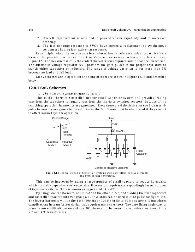
346 Extra High Voltage AC Transmission Engineering
7. Overall improvement is obtained in power-transfer capability and in increasedeconomy.
8. The fast dynamic response of SVC's have offered a replacement to synchronouscondensers having fast excitation response.
In principle, when the voltage at a bus reduces from a reference value, capacitive Varshave to be provided, whereas inductive Vars are necessary to lower the bus voltage.Figure 12.14 shows schematically the control characteristics required and the connection scheme.The automatic voltage regulator AVR provides the gate pulses to the proper thyristors toswitch either capacitors or inductors. The range of voltage variation is not more than 5%between no load and full load.
Many schemes are in operation and some of them are shown in Figure 12.15 and describedbelow.
12.8.1 SVC Schemes1. The TCR-FC System (Figure 12.15 (a)).
This is the Thyristor Controlled Reactor-Fixed Capacitor system and provides leadingvars from the capacitors to lagging vars from the thyristor-switched reactors. Because of theswitching operation, harmonics are generated. Since there are 6 thyristors for the 3-phases, 6-pulse harmonics are generated in addition to the 3rd. These must be eliminated if they are notto affect normal system operation.
Fig. 12.14 General circuit of Static Var Systems with controlled reactive elementsand control range exercised.
This can be improved by using a large number of small reactors to reduce harmonicswhich normally depend on the reactor size. However, it requires correspondingly larger numberof thyristor switches. This is known as segmented TCR-FC.
By using two transformers, one in Y/∆ and the other in Y/Y, and dividing the fixed capacitorsand controlled reactors into two groups, 12 thyristors can be used in a 12-pulse configuration.The lowest harmonic will be the 12th (600 Hz or 720 Hz in 50 or 60 Hz system). It introducescomplications in transformer design, and requires more thyristors. The gate-firing angle controlis made more difficult because of the 30° phase shift between the secondary voltages of theY/∆ and Y/Y transformers.
Control Range
VREF
BusVoltage
CapacitiveMVAR
InductiveMVAR
x CB
Line
TRANS
Fixed Capacitor
AVR
Controlled Reactive Elements
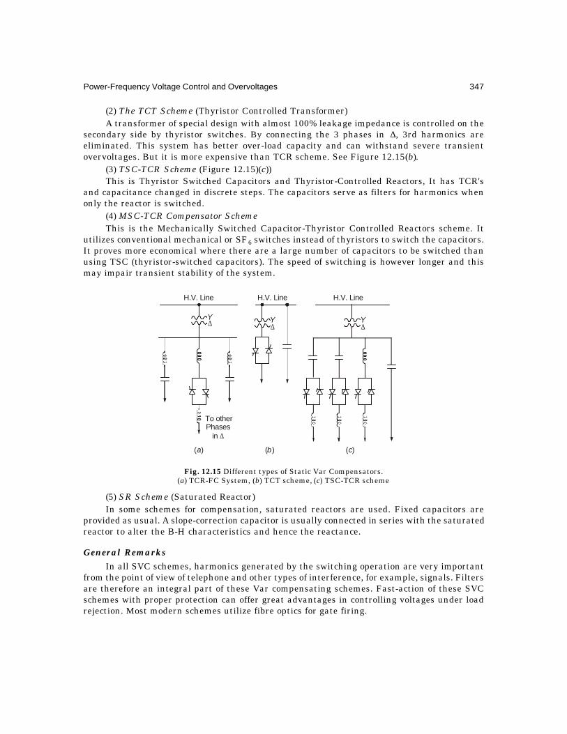
Power-Frequency Voltage Control and Overvoltages 347
(2) The TCT Scheme (Thyristor Controlled Transformer)A transformer of special design with almost 100% leakage impedance is controlled on the
secondary side by thyristor switches. By connecting the 3 phases in ∆, 3rd harmonics areeliminated. This system has better over-load capacity and can withstand severe transientovervoltages. But it is more expensive than TCR scheme. See Figure 12.15(b).
(3) TSC-TCR Scheme (Figure 12.15)(c))This is Thyristor Switched Capacitors and Thyristor-Controlled Reactors, It has TCR's
and capacitance changed in discrete steps. The capacitors serve as filters for harmonics whenonly the reactor is switched.
(4) MSC-TCR Compensator SchemeThis is the Mechanically Switched Capacitor-Thyristor Controlled Reactors scheme. It
utilizes conventional mechanical or SF6 switches instead of thyristors to switch the capacitors.It proves more economical where there are a large number of capacitors to be switched thanusing TSC (thyristor-switched capacitors). The speed of switching is however longer and thismay impair transient stability of the system.
Fig. 12.15 Different types of Static Var Compensators.(a) TCR-FC System, (b) TCT scheme, (c) TSC-TCR scheme
(5) SR Scheme (Saturated Reactor)In some schemes for compensation, saturated reactors are used. Fixed capacitors are
provided as usual. A slope-correction capacitor is usually connected in series with the saturatedreactor to alter the B-H characteristics and hence the reactance.
General Remarks
In all SVC schemes, harmonics generated by the switching operation are very importantfrom the point of view of telephone and other types of interference, for example, signals. Filtersare therefore an integral part of these Var compensating schemes. Fast-action of these SVCschemes with proper protection can offer great advantages in controlling voltages under loadrejection. Most modern schemes utilize fibre optics for gate firing.
H.V. Line H.V. Line H.V. Line
To otherPhases
in ∆
∆ ∆ ∆Y Y Y
( )a ( )b ( )c

348 Extra High Voltage AC Transmission Engineering
The current-voltage relationships as a function of firing angle are shown in Figure 12.16(a)and (b) for switched reactors and capacitors respectively.
A complete 3-phase bank of switched reactor or capacitor connected in ∆ is schematicallyshown in Figure 12.16, which eliminates triplen harmonics.
Fig. 12.16. Voltage-current relationships in switched reactor and capacitorwith variation in firing angle α.
12.8.2 Harmonics Injected into Network by TCRFigure 12.17 shows filter capacitors and the TCR's connected to the low-voltage winding of astep-down transformer. This may be a 2-winding or in most cases a 3-winding transformerhaving primary, secondary and low-voltage tertiary. We will analyse the problem of harmonicgeneration, filter design and the resulting harmonic injection into the system through thetransformer windings. When the TCR's are connected in ∆, the 3rd harmonic and its multiplesare eliminated. The low-voltage winding feeding the TCR's may be connected either in ∆ or Yas shown in Figure 12.18. The harmonics present are therefore of orders 5, 7, 11, 13, etc., thatis (2n ± 1) times the fundamental where n = 3k, k = 1, 2, 3,... This gives rise to both positive-sequence and negative-sequence currents.
The amplitude of a harmonic depends entirely on the firing angle of the thyristors, denotedby α. Since the current is purely inductive, it will lag behind the transformer voltage by 90° inso far as the fundamental is concerned. For full conduction, α = 90° from a voltage zero.Figure 12.19 shows the relation between voltage and current for α = 90° and for α > 90°. Whenα = 90°, no harmonics are generated, obviously. For a general value of α, the fundamentalcomponent of current is
I1 = ∫α−π
α
α−π−α−π
π=θθθ
π)(2sin
212
sin.sin2
IdI ...(12.70)
When II =π=α 1,2/ in equation (12.70) so that the value I can be considered as the
amplitude of the fundamental when the reactors are conducting fully over the entire cycle.
V
L
I
V
C
I
V
I
α = 90°120°90°
V
Iα = 90°120°
(a)
(b)

Power-Frequency Voltage Control and Overvoltages 349
When α changes, the amplitude of fundamental also changes, which is as shown in the followingtable and calculated from equation (12.70):
α = 90° 105° 120° 135° 150° 165° 180°I1/I = 1 0.674 0.391 0.182 0.058 0.0075 0
Fig. 12.17 Harmonic injection by TCR into a high-voltage system through 2-windingand 3-winding transformers.
Fig. 12.18 Connection of TCR to ∆ and Y-connected transformer windings.
Fig. 12.19 Voltage waveform and current waveforms for α = 90° (full conduction of TCR) and α > 90°, forcalculation of harmonics. (I90 = current under full conduction of thyristor and no harmonics).
H.V. Line
P P SS T
TCR TCR
H.V. Line M.V. Line
Trans TCR Trans TCR
α90°
180°–α
V
I = I90
Iα
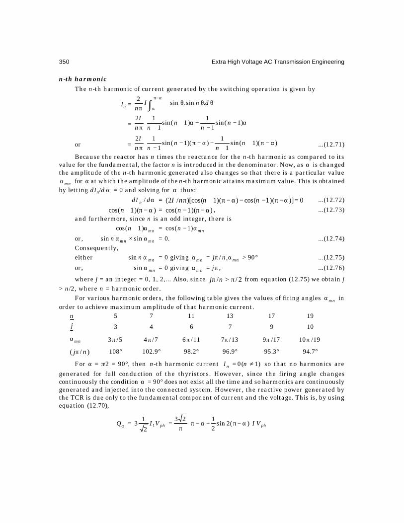
350 Extra High Voltage AC Transmission Engineering
n-th harmonic
The n-th harmonic of current generated by the switching operation is given by
In = ∫α−π
αθθθ
πdnI
n.sin.sin
2
=
α−
−−α+
+π)1sin(
11
)1sin(1
12n
nn
nnI
or =
α−π+
+−α−π−
−π))(1sin(
11
))(1sin(1
12n
nn
nnI
...(12.71)
Because the reactor has n times the reactance for the n-th harmonic as compared to itsvalue for the fundamental, the factor n is introduced in the denominator. Now, as α is changedthe amplitude of the n-th harmonic generated also changes so that there is a particular value
mnα for α at which the amplitude of the n-th harmonic attains maximum value. This is obtainedby letting dIn/d α = 0 and solving for α thus:
αddI n / = 0)])(1cos())(1)[cos(/2( =α−π−−α−π+π nnnI ...(12.72)
∴ ))(1cos( α−π+n = ))(1cos( α−π−n , ...(12.73)and furthermore, since n is an odd integer, there is
mnn α+ )1cos( = mnn α− )1cos(
or, mnmnn α×α sinsin = 0. ...(12.74)Consequently,either mnn αsin = 0 giving °>απ=α 90,/ mnmn nj ...(12.75)
or, mnαsin = 0 giving π=α jmn , ...(12.76)
where j = an integer = 0, 1, 2,... Also, since 2// π>π nj from equation (12.75) we obtain j> n/2, where n = harmonic order.
For various harmonic orders, the following table gives the values of firing angles mnα inorder to achieve maximum amplitude of that harmonic current.
n 5 7 11 13 17 19
j 3 4 6 7 9 10
mnα 5/3π 7/4π 11/6π 13/7π 17/9π 19/10π
)/( njπ 108° 102.9° 98.2° 96.9° 95.3° 94.7°
For α = π/2 = 90°, then n-th harmonic current )1(0 ≠= nIn so that no harmonics are
generated for full conduction of the thyristors. However, since the firing angle changescontinuously the condition α = 90° does not exist all the time and so harmonics are continuouslygenerated and injected into the connected system. However, the reactive power generated bythe TCR is due only to the fundamental component of current and the voltage. This is, by usingequation (12.70),
αQ = phph VIVI
α−π−α−π
π= )(2sin
2123
2
13 1
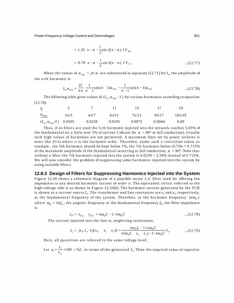
Power-Frequency Voltage Control and Overvoltages 351
= phVI
α−π−α−π )(2sin
21
35.1
= llVI −
α−π−α−π )(2sin
21
78.0 ...(12.77)
When the values of njmn /π=α are substituted in equation (12.71) for In, the amplitude of
the n-th harmonic is
In,αmn =
α−
−−α+
+π mnmn nn
nnn
I)1sin(
11
)1sin(1
12...(12.78)
The following table gives values of )/,( II mnn α for various harmonics according to equation
(12.78):n 5 7 11 13 17 19
mnα 5/3π 7/4π 11/6π 31/7π 71/9π 91/10π
)/,( II mnn α 0.0505 0.0259 0.0105 0.0075 0.0044 0.00
Thus, if no filters are used the 5-th harmonic injected into the network reaches 5.05% ofthe fundamental (or a little over 5% of current I obtain for α = 90° or full conduction). Usuallysuch high values of harmonics are not permitted. A maximum limit set by power utilities ismore like (5/n) where n is the harmonic order. Therefore, under such a restriction taken asexample , the 5th harmonic should be kept below 1%, the 7th harmonic below (5/7)% = 0.715%of the maximum amplitude of the fundamental occurring at full conduction, α = 90°. Note thatwithout a filter the 7th harmonic injected into the system is 0.0259 = 2.59% instead of 0.715%.We will now consider the problem of suppressing some harmonics injected into the system byusing suitable filters.
12.8.3 Design of Filters for Suppressing Harmonics Injected into the SystemFigure 12.20 shows a schematic diagram of a possible series L-C filter used for offering lowimpedance to any desired harmonic current of order n. The equivalent circuit referred to thehigh-voltage side is as shown in Figure 12.20(b). The harmonic current generated by the TCRis shown as a current source In. The transformer and line reactances are xt and xl, respectively,at the fundamental frequency of the system. Therefore, at the harmonic frequency )( 0ωnwhere 00 2 fπ=ω , the angular frequency at the fundamental frequency f0, the filter impedanceis
xF = CnLnxx FCFL 00 /1 ω−ω=+ ...(12.78)
∴ The current injected into the line is, neglecting resistances,
I1 = nlt
ltFnF ICnxxLn
CnLnxxxjIjx
00
00
/1)(/1
)](/[ω−++ω
ω−ω=++ ...(12.79)
Here, all quantities are referred to the same voltage level.
Let ln
l III
%100 =×=η in terms of the generated In. Then the required value of capacitor

352 Extra High Voltage AC Transmission Engineering
can be found out for a set limiting value η for the harmonic. In the previous section this limitwas taken to be (5/n)%. If a = turns ratio of the transformer, then
100η
=FltF
FF
CnaxxaLnaCnLn
022
0
200
/)(
)/1(
ω−++ωω−ω
...(12.80)
where LF, CF = actual values of filter inductance and capacitance connected to the low-voltage winding of the step-down transformer, and xt, xl are actual values of transformer andline reactances referred to the high-voltage side at the fundamental frequency f0 or angularfrequency ω0. Examples will make clear the design and operation of the filter for a given simplesystem.
Fig. 12.20 Arrangement of TCR and filter for suppression of harmonics.(a) Actual connection to transformer secondary.(b) Inductive and capacitive reactances referred
to primary by turns ratio a.
Example 12.16. A 100 MVA 230 kV 50 Hz transformer has xt = 12% and is connected to aline 200 km long which has an inductance of 1 mH/km. The filter, connected to the l.v. 33 kVside of the transformer, is required to suppress the 5-th harmonic generated by the TCR to 1%of In. Calculate the value of filter capacitor if the filter inductance used is 2 mH.
Solution. The given data are:xt = 0.12 × 2302/100 = 63.48 ohmsxl = 314 × 0.2 = 62.8 ohmsa = 230/33 = 6.97
FL0ω = 314 × 2 × 10–3 = 0.628 ohm at 50 Hz.
η = 1% = 0.01.n = 5-th harmonic = 5.
∴ From equation (12.80)
0.01 =F
F
CC
1570/97.6)8.6248.6397.6628.0(5
97.6)1570/1628.05(22
2
−++×−×
H.V. Bus
PS Ratio, a
Turns
LFTCR
CF
H.V.
a w C2 0/ F
a w L20 F
( )b
( )a
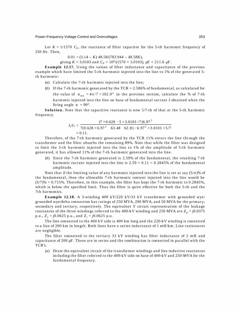
Power-Frequency Voltage Control and Overvoltages 353
Let K = 1/1570 CF, the reactance of filter capacitor for the 5-th harmonic frequency of250 Hz. Then,
0.01 = (3.14 – K) 48.58/(783.944 – 48.58K),giving K = 3.0103 and CF = 106/(1570 × 3.0103), µF = 211.6 µF.
Example 12.17. Using the values of filter inductance and capacitance of the previousexample which have limited the 5-th harmonic injected into the line to 1% of the generated 5-th harmonic:
(a) Calculate the 7-th harmonic injected into the line;
(b) If the 7-th harmonic generated by the TCR = 2.586% of fundamental, as calculated for
the value of °=π=α 9.1027/4mn in the previous section, calculate the % of 7-th
harmonic injected into the line on base of fundamental current I obtained when thefiring angle α = 90°.
Solution. Note that the capacitive reactance is now 5/7-th of that at the 5-th harmonicfrequency.
Il/I7 = 7/50103.397.6)8.6248.6397.6628.0(7
97.6)7/0103.35628.07(22
2
××−++×
×−×
= 0.11.Therefore, of the 7-th harmonic generated by the TCR 11% enters the line through the
transformer and the filter absorbs the remaining 89%. Note that while the filter was designedto limit the 5-th harmonic injected into the line to 1% of the amplitude of 5-th harmonicgenerated, it has allowed 11% of the 7-th harmonic generated into the line.
(b) Since the 7-th harmonic generated is 2.59% of the fundamental, the resulting 7-thharmonic current injected into the line is 2.59 × 0.11 = 0.2845% of the fundamentalamplitude.
Note that if the limiting value of any harmonic injected into the line is set at say (5/n)% ofthe fundamental, then the allowable 7-th harmonic content injected into the line would be(5/7)% = 0.715%. Therefore, in this example, the filter has kept the 7-th harmonic to 0.2845%,which is below the specified limit. Thus the filter is quite effective for both the 5-th and the7th harmonics.
Example 12.18. A 3-winding 400 kV/220 kV/33 kV transformer with grounded wye/grounded wye/delta connection has ratings of 250 MVA, 200 MVA, and 50 MVA for the primary,secondary and tertiary, respectively. The equivalent Y circuit representation of the leakagereactances of the three windings referred to the 400-kV winding and 250 MVA are Zp = j0.0375p.u., Zs = j0.0625 p.u., and Zt = j0.0625 p.u.
The line connected to the 400 kV side is 400 km long and the 220-kV winding is connectedto a line of 200 km in length. Both lines have a series inductance of 1 mH/km. Line resistancesare negligible.
The filter connected to the tertiary 33 kV winding has filter inductance of 2 mH andcapacitance of 200 µF. These are in series and the combination is connected in parallel with theTCR's.
(a) Draw the equivalent circuit of the transformer windings and line inductive reactancesincluding the filter referred to the 400-kV side on base of 400-kV and 250-MVA for thefundamental frequency.
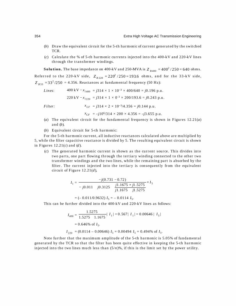
354 Extra High Voltage AC Transmission Engineering
(b) Draw the equivalent circuit for the 5-th harmonic of current generated by the switchedTCR.
(c) Calculate the % of 5-th harmonic currents injected into the 400-kV and 220-kV linesthrough the transformer windings.
Solution. The base impedance on 400-kV and 250-MVA is 640250/4002400 ==BZ ohms.
Referred to the 220-kV side, 6.193250/2202220 ==BZ ohms, and for the 33-kV side,
250/33233 =BZ = 4.356. Reactances at fundamental frequency (50 Hz):
Lines: 400kV400 lx− = j314 × 1 × 10–3 × 400/640 = j0.196 p.u.
220kV220 lx− = j314 × 1 × 0–3 × 200/193.6 = j0.243 p.u.
Filter: LFx = j314 × 2 × 10–3/4.356 = j0.144 p.u.
CFx = –j106/314 × 200 × 4.356 = –j3.655 p.u.
(a) The equivalent circuit for the fundamental frequency is shown in Figures 12.21(a)and (b).
(b) Equivalent circuit for 5-th harmonic:For the 5-th harmonic current, all inductive reactances calculated above are multiplied by
5, while the filter capacitive reactance is divided by 5. The resulting equivalent circuit is shownin Figures 12.21(c) and (d).
(c) The generated harmonic current is shown as the current source. This divides intotwo parts, one part flowing through the tertiary winding connected to the other twotransformer windings and the two lines, while the remaining part is absorbed by thefilter. The current injected into the tertiary is consequently from the equivalentcircuit of Figure 12.21(d),
I1 = 5
5275.11675.15275.11675.1
3125.0011.0
)72.0731.0(I
jjjjjj
j×
+×++−
−−
= (– 0.011/0.9632) I5 = – 0.0114 I5.
This can be further divided into the 400-kV and 220-kV lines as follows:
I400 = ||00646.0||567.0||1675.15275.1
5275.1511 III ==
+
= 0.646% of I5.
220I = (0.0114 – 0.00646) I5 = 0.00494 I5 = 0.494% of I5.
Note further that the maximum amplitude of the 5-th harmonic is 5.05% of fundamentalgenerated by the TCR so that the filter has been quite effective in keeping the 5-th harmonicinjected into the two lines much less than (5/n)%, if this is the limit set by the power utility.
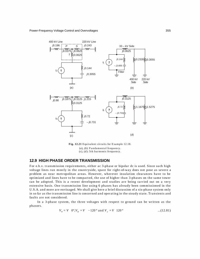
Power-Frequency Voltage Control and Overvoltages 355
Fig. 12.21 Equivalent circuits for Example 12.18.
(a), (b): Fundamental frequency.(c), (d): 5th harmonic frequency.
12.9 HIGH PHASE ORDER TRANSMISSIONFor e.h.v. transmission requirements, either ac 3-phase or bipolar dc is used. Since such highvoltage lines run mostly in the countryside, space for right-of-way does not pose as severe aproblem as near metropolitan areas. However, wherever insulation clearances have to beoptimized and lines have to be compacted, the use of higher than 3-phases on the same towercan be adopted. This is a recent development and studies are being carried out on a veryextensive basis. One transmission line using 6 phases has already been commissioned in theU.S.A. and more are envisaged. We shall give here a brief discussion of a six-phase system onlyin so far as the transmission line is concerned and operating in the steady state. Transients andfaults are not considered.
In a 3-phase system, the three voltages with respect to ground can be written as thephasors.
Va = °∠=°−∠=°∠ 120and120,0 VVVVV cb ...(12.81)
j0.196
j0.0375 j0.0625
j0.0625
j0.144
j0.3055I1
j0.243400 kV Line 220 kV Line
P S
T
( )a
j0.98 j0.1875 j0.3125 j1.215
j0.3125
j0.72
– j0.731I5
( )c
I5
j0.3125
j1.5275j1.1675
( )d
j0.72
– j0.731
I1
Filter
33 – kV Side
j0.0625
j0.3055j0.2335
400 kVSide
220 kVSide
( )b
j0.144
– j3.655

356 Extra High Voltage AC Transmission Engineering
The magnitude of line-to-line voltages are also equal so that
|Vab| = |Vbc| = |Vca| = V3 .When a double-circuit configuration is used, as shown in Figure 12.22(a), we observe that
the insulation clearance between the conductors are nearly
ac'D = ,, hDDDDDDD a'b'b'c'bcabca'bb' ======
Dac = hDa'c' 2= , and so on.On the other hand, the magnitude of voltages are
ac'V = ;3VVVVVV a'b'b'c'bcabca' =====
aa'V = 0== cc'bb' VV and so on.Comparing the insulation clearances with the voltages (neglecting the tower width) we
observe that they bear no relation to each other. Thus, spatial distribution of insulationclearances do not match the voltages experienced by them. Therefore, the line is not optimizedto this extent.
Fig. 12.22 Double-circuit 3-phase ac line and single-circuit 6-phase line.
Now consider the situation when the six conductors are energized by a 6-phase system ofvoltages, Figure 12.22(b). These are
Also
−=−=−=°−∠=°−∠=°−∠=
°−∠=°−∠=°∠=
362514
654
321
,,
300,240,180
,120,60,0
VVVVVVVVVVVV
VVVVVV
...(12.82)
These are voltages to ground. The corresponding magnitudes of voltages between conductorsare as follows:
===
======
======
.2
3
362514
625146352413
615645342312
VVVV
VVVVVVV
VVVVVVV
...(12.83)
From Figure 12.22(b) it may be observed that the distances between the pairs of conductorsdenoted by the subscripts in equation (12.82) in the voltages are also equal to the correspondingvoltage magnitudes. Thus, the spatial distribution of conductors corresponds to the distribution
1
2
3 4
5
6
D
D'
D
h
h
a a'
b b'
c c'
(a) (b)
D/C 3-Phase S/C 6-Phase

Power-Frequency Voltage Control and Overvoltages 357
of system voltages. Insulation clearances are optimized to a high degree and the lines can becompacted better than in a double-circuit 3-phase line.
For system voltages (line-to-ground) ranging from 80 kV to 442 kV, the voltages betweenadjacent phases in a 3-phase system and a 6-phase system are compared in the following table.
Phase-Ground Voltage, kV 80 133 199 230 289 442Phase-Phase Voltage, kV 3-phase 138 230 345 400 500 765(Between adjacent 6-phase 80 133 199 230 289 442Conductors)
We observe that it is better to define the phase-to-ground voltage as the system voltagesince this is a common factor for both 3-phase and 6-phase system. The voltage between conductorsis in the ratio 3:1 for the 6-phase and 3-phase systems and insulation clearances are smallerfor the 6-phase system. This results in a great reduction in overall dimensions of the towers.
Fig. 12.23 Several alternative configurations for high phase order 6-phase line on tower.
Some of the proposed conductor configurations for 6-phase systems are depicted inFigure 12.23.
Comparison of Power-Handling CapacityFor the sake of comparison, we assume that a double-circuit 3-phase system and a 6-
phase system have the same conductor size and line-to-ground voltages. Therefore, the currentper conductor is assumed the same for both systems. Then, the following power relations hold:
××=−
××=−
CLGph
CLGph
IVPSystemCSPhase
IVPSystemCDPhase
6/6
6/3
6
3...(12.84)
Therefore, cost for cost, there is no difference between the two systems as long as theline-to-ground voltages are equal and the current-carrying capacities of the conductors are alsoequal.
D
D
D
D
DD
D
D

358 Extra High Voltage AC Transmission Engineering
Other FactorsFor medium-voltage lines up to 138 kV, 3-phase, (80 kV line-to-ground) and 6-phase 80 kV lines,with 1 metre clearance between adjacent conductors in the 6-phase system, the clearancebetween conductors in the 3-phase system will be 1.73 metres. As an example, with both havingconductors of 2.3 cm diameter, the maximum surface voltage gradients on the conductors are:
3-phase system – 12 kV/cm (r.m.s.)6-phase system – 10.5 kV/cm (r.m.s.)
Ground-level electrostatic fields (See Chapter 7) with 11-metre height of lowest conductorabove ground are both less than 1 kV/m so that this is not a point of much concern.
Review Questions and Problems
1. Derive equations (12.1) and (12.2) for the voltage and current at any point on atransmission line in terms of the voltage at entrance to the line.
2. A 750 kV line has the distributed line constants r = 0.025 ohm/km, l = 0.9 mH/km,and c = 12.3 nF/km. At 50 Hz, calculate the following if the line is 600 km in length.
(a) A, B, C, D constants.
(b) The charging current and MVAR at a receiving end voltage of 750 kV, line-line,on no load.
(c) The coordinates of the centre of the receiving end power-circle diagram.
(d) The surge-impedance loading.
3. In Example 12.13, the shunt reactor compensation for maintainingEs = 726 kV and Er = 765 kV, for a 750 kV
line, reactors had 3-phase ratings of 335 MVAR and 372 MVAR. With the sending-endvoltage held constant at 726 kV, there is a total loss of reactor at the receiving enddue to a fault. Calculate the receiving-end voltage resulting from taking the reactorout of service.
4. Repeat problem 3 if the reactors at both ends are taken out of service. Calculate thevoltage at the receiving end with Es = 726 kV.
5. Derive equations (12.63) and (12.64).
6. A very long line has series capacitance amounting to 50% of the series reactance.Calculate the natural electrical frequency.
7. List the dangers resulting from series capacitor compensation on long lines, and theremedies taken to counteract them.
8. What is the reason for the existence of SSR in the steady state and transient conditionsin series-capacitor compensated lines?
9. List 3 dangerous conditions which give rise to SSR and all the countermeasurestaken to guard against them. Use a tabular form.

13.1 STANDARD SPECIFICATIONSAll e.h.v. equipment voltage levels are governed by Standard Specifications adopted in eachcountry. Equipment manufacturers produce goods not only for domestic use but also for exportso that a design or testing engineer must be familiar with these specifications from all over theworld. Some of the major specifications are I.E.C., I.S.I., V.D.E., S.A.E., A.N.S.I., B.S.S., C.S.A.,U.S.S.R., Japan and others. In this chapter we shall discuss some of the requirements of e.h.v.insulation levels conforming to Indian Standards which parallel the I.E.C, specifications formost types of equipment and lines.
Standard VoltagesAt and above 220 kV, the voltage levels that must not be exceeded in any part of the system arestipulated by IS 2026: Specifications for Power Transformer–Part III: Insulation Levels andDielectric Tests. Some typical values are quoted on next page.
Certain broad outlines can be discussed here regarding the voltages levels. With increasingthickness used for solid insulation structures in transformers immersed in oil, the danger ofvoids forming in the insulation is increased. For lower-voltage transformers, a test at twice therated maximum voltage at double the power frequency for 60 seconds was specified without theneed for partial-discharge measurement. However, at higher voltages the test voltage is 150%of maximum equipment voltage and the duration of voltage is increased to 30 minutes with theneed for detection of partial discharges. From volt-time experiments carried out on such insulationstructures, it has been ascertained that a transformer which does not show a failure underthese test conditions can be expected to have reasonably long life if maintenance is excellentduring service.
We also observe several levels of P.F., switching, and lightning-impulse withstand testvoltages. These are necessary in view of the severity or otherwise of these voltages occurringin practice. For example, a transformer located in regions of high isokeraunik level should betested at the higher test voltage level.
13EHV Testing and Laboratory Equipment

360 Extra High Voltage AC Transmission Engineering
1. Nominal System 220 275 345 400 500 750kV, RMS (l – l)
2. Highest Equipment 245 300 362 420 525 765kV, RMS
3. Short Duration P.F. 325 395,460 460,510 570,630 790 1150Withstand Voltage 360kV, RMS 395
4. Rated Switching 750,850 850,950 950,1050 1050,1175 1425,1550Impulse WithstandVoltage, kV crest
5. Rated Lightning 750 850,950 950,1050 1050,1175 1175,1425 1550,1800Impulse Withstand 850 950,1050 1050,1175 1175,1300 1300,1550 1800,1950Voltage, kV crest 950 1425 1425
Note that there are several levels of P.F. voltages, lightning-impulse voltages andswitching-surge withstand voltages.
Typical values of interest are as follows:
Arrester Withstand Voltage Impulse Sparkover kV, crestVoltage up to 10 kA (1.2/50 µs), kV, Crest Residual VoltageRating Arresters
kV, RMS 10 kA Front of the wave,kV/ µs
150 288 500/577 at 1080 500174 334 570/660 1160 570186 356 610/702 1180 610198 380 649/746 1200 649
>198 1.9 × RatedArrester Voltage
To 225 3.28/3.78 1200 3.28 × Rated VoltageRated Voltage
To 396 3.26/3.76 1200 3.26 × Rated VoltageRated Voltage
>396 No values are 1200 No values areagreed upon specified
Lightning ArrestersGapless type arresters are new and standard specifications are still being formulated. But forgap-type non-linear resistor type arresters, typical test values are given in IS 3070-Part I (1974),revised in 1982.
Three important items specified are
1. Voltage withstand of the series gap;
2. Maximum impulse sparkover of the gap;
3. Maximum residual voltage of the resistor block.

EHV Testing and Laboratory Equipment 361
The standard lightning-impulse waveshapes are (a) 1.2/50 µs for voltage, (b) 8/20 µs forcurrent. These timings and their definitions will be described later.
In addition, a long-duration impulse current test is also required at 150 Ampere peakcurrent for 2000 µs duration (of the peak) for 10 kA class of arresters. This simulates switchingsurges on lines.
A high-voltage laboratory should consist of sources or generators to provide the necessarytest voltages, and in addition, be adequate to carry out research and development work. Theremaining parts of this chapter will be devoted to description and design of these testingequipments.
13.2 STANDARD WAVESHAPES FOR TESTINGThe transient voltages impinging on equipment when connected in a system show a widevariation in magnitude and waveshape. It is only the power-frequency voltage which has adefinite sinusoidal shape and is symmetric in both half cycles. However, from a vast experienceand amount of experimental data collected, it has been ascertained that the severity of stresson the equipment insulation is properly represented during testing if these voltages and currentsare standardized regarding their magnitudes and waveshapes. The magnitudes have alreadybeen given through examples from standard specifications. The waveshapes are discussed below.Their generation in a laboratory will be described later on.
13.2.1 Voltage Waveshapes
(1) Lightning Impulse
For testing all types of equipment including transformers under lightning impulses, thefollowing definition for voltage will be used as per I.E.C. and Indian Standard Specifications asshown in Figure 13.1. In this waveform Vp = crest value, V0 = over-shoot, tm = time to crest, tt= time to 50% value on tail, t1 = time to 90% value of crest, t2 = time to 30% value of crest, 0 =actual zero, 0' = virtual zero. All timings are measured from the virtual zero 0', which isdefined below.
Fig. 13.1 Details of lightning-impulse voltage waveshape.
The solid curve represents the actual desired waveshape generated without oscillationson the front, and without the overshoot shown by broken line. The wave can be expressed asthe difference between two exponentials with equation.
e(t) = )( tt eeE β−α− − ...(13.1)
tmt1
t2
Overshoot
Vp
0.9Vp
0.5Vp
0.3Vp
0'
0
tt

362 Extra High Voltage AC Transmission Engineering
There is an initial curvature at the wavetoe, followed by a nearly linear rise, then a verygradual rise to peak value, and finally a fall to zero value on the 'tail'. The important timingsare:
(1) the time interval between 90% and 30% crest value, t1 – t2,(2) the virtual zero of time (point 0') obtained by joining the 90% and 30% voltages and
extending it backwards to intersect the time axis (zero voltage),
(3) the tim e tm from virtual zero to crest value,
(4) the time tt from 0' to 50% crest value on the tail,
(5) the time interval t3 during which the voltage remains above 90% crest value.On the same figure is shown an oscillatory portion with an overshoot V0 since the presence
of inductance in a two-element energy storage circuit with small damping gives rise to oscillationsat the peak value.
The standard waveshape defined above has the following specifications for the timingsand overshoot:
Front time: tf = 1.67 (t1 – t2) = 1.2 µs ± 30% tolerance= 0.84 µs to 1.56 µs.
Tail time: tt = 50 µs ± 20% tolerance = 40 µs to 60 µs.Overshoot : Not over 5% of crest value.In normal laboratory-generated waves, the virtual zero occurs in less than 0.2 µs from the
actual zero 0. The time to actual crest from zero, tm, is in general twice the front time tf.However, the actual value will depend on the waveshape timings with their tolerance and willbe discussed later on.
(2) Switching Surge for Testing Line EquipmentFor testing all equipment other than transformer under switching surge voltages, the
front and tail timings for the double-exponential waveshape of Figure 13.1 have the followingvalues and tolerances:
Front Time: tf = sstt µ=±µ=− 325to175%30250)(67.1 21
Tail Time: tt = ss µ=±µ 3000to2000%202500 .
For crest values longer than 100 ,sµ certain standard specifications permit the front timeof 250 sµ to equal the time to actual crest value of voltage. The test engineer must consult thestandards for such variations allowed in definitions.
(3) Switching Surge for Transformer Testing
On account of the large inductance which an unloaded transformer presents to a high-voltage generator, oscillations result on the wavetail. For this reason, standards specify thefollowing definitions for a switching surge for transformer testing: As per Indian Standards, thewavefront should be at least 20 ,sµ the length of surge from first zero to the occurrence of nextzero must be at least 500 ,sµ and the magnitude of the surge must be in excess of 90% of crestvalue for at least 200 .sµ When core saturation occurs the length of the surge may be shorter
than 500 ,sµ but this is usually corrected by injecting a dc of proper polarity in special tests.

EHV Testing and Laboratory Equipment 363
Fig. 13.2 Details of lightning-current waveshape.
13.2.2 Current WaveshapesFor type testing lightning arresters, the lightning current impulse wave-shapes have the followingspecifications, as shown in Figure 13.2:
(1) Short – Duration Impulse. Time to crest = 8 ,sµ on a straight line joining 10% and90% crest values. Time to 50% value on tail = 20 .sµ
(2) Long – Duration Impulse. Time duration of crest value is 1000 sµ to 2000 sµ dependingupon the crest value of current. For 150 Amps, the duration is 2000 sµ and for light-duty arresters for 100 Amps, it is 1000 .sµ
Most of the voltage and current waveshapes of double-exponential types are generated byusing capacitors, resistors, cascade-connected testing transformers. But the long-duration currentwave is generated by a set of inductors and capacitors which represent a transmission line typeof circuit.
13.3 PROPERTIES OF DOUBLE–EXPONENTIAL WAVESHAPESA double exponential voltage waveshape can be generated in principle by charging a capacitorand discharging it through properly-connected set of resistors and a load capacitance. Thecircuit description and design of such generators based on the principle of the Marx circuit willbe discussed in the next section. Here, we shall describe the properties of a double exponentialwaveshape which form the basis for designing the generator or modifying them in order toobtain suitable waveshapes for standard test as well as for research and development purposes.
The waveshape and its important properties are shown in Figure 13.The equation is
e(t) = )( tt eeE β−α− − ...(13.1)
Ip0.9Ip
0.5Ip
0.1Ip0
0'
20 sµ
8
1000 to2000 sµ
Ip
t0

364 Extra High Voltage AC Transmission Engineering
The required properties are(a) the crest value Vp,(b) the front time
tf = )(67.1)(6.0
1309021 tttt −=− ...(13.2)
(c) the tail time tt.
The value of E in equation (13.1) in relation to the crest Vp will depend on the requiredtimings for the voltage. The standard timings are
(a) for lightning, tf = sts t µ±=µ± 1050,36.02.1 .
(b) for switching, tf = sts t µ±=µ± 5002500,75250 .
The values of α and β will be controlled by these timings, and vice versa.
Example 13.1. Examine the double-exponential waveshape for tf tt , , and Vp given that E= 1.035, α = 14.5 × 10³, and β = 2.45 × 10⁶.
Solution. Normally, since t is in microseconds, we modify the values of α and β suitably.The given equation can be re-written as )(035.1)( 45.20145.0 tt eete −− −= with t in µs.
For examining the wavefront, let t range from 0 to 1 µs. Then the following values areobtained.
t = 0.1 0.15 0.2 0.4 0.6 0.8 0.85 0.9 1.0e = 0.2234 0.316 0.398 0.64 0.788 0.877 0.893 0.9074 0.9315
At t = 0.141, e = 0.3, and at t = 0.87, e = 0.9.∴ The front time is
tf = 1.67 (0.87 – 0.141) = 1.215 µs.
At t = 50 µs, the voltage is e = 0.501. Therefore, the given values of E, α and β satisfy therequirements for a standard 1.2/50 µs waveshape. The peak value Vp = 1 is obtained at t = 2.22 µs.
Example 13.2. Given E = 1.13, α = 326, and β = 11 × 103, examine the waveshape
e = )(13.131011326 tt ee ×−×− − for a switching impulse.
Solution. At t = 3.0sec,102929 6 =×=µ − esAt t = 9.0sec,10172172 6 =×=µ − es∴ tf = 1.67 (172 – 29) = 238 µs.At t = 2500 µs, e = 0.5.These fall within the required tolerances. The wave reaches a peak value of 0.985 at 360 µs.
13.3.1 Lightning Impulses: Values of E, αα , ββFor design purposes, Figure 13.3 (a), (b), (c) provide information about the three parameters inequation (13.1) for timings. The method of calculating these is quite lengthy and will be outlinedin section 13.4 next. It requires the solution of a set of non-linear equations and has beencarried out by an iteration procedure using the Digital Computer. Simplified methods yieldingquick results for engineering purposes will also be discussed later.
tf = 1.2 ± 30% and tt = 50 ± 20% µs

EHV Testing and Laboratory Equipment 365
Fig. 13.3 Variation of E, α, β of a double-exponential voltage wave of lightning type with front tfThe tail time tt is used as parameter.
13.3.2 Switching Impulses: Values of E, α, βα, βFor tf = 125 to 500 µs and tt = 2000 to 5000 µs,
the range of variation of E, α and β is shown in Figure 13.4.
Fig. 13.4 Variation of E, α, β for switching-impulse type of voltage wave with front time tf.
Fig. 13.5 Variation of time to crest tm of a double-exponential waveform with front and tail timings.
1.000
1.025
1.050
1.075
EV/
p
t sf,µ40
5060
0.8 1.0 1.2 1.4 1.6t sf, µ
t st,µ19
1817
1615
14
1312
11
40
45
50
60
0.8 1.0 1.2 1.4 1.6
× 103
t sf, µ
α
0.8 1.0 1.2 1.4 1.8
4.0
3.5
3.0
2.5
2.0
1.5
× 106
t st, µ
t sf, µ
5040
β
1.4
1.3
1.2
1.1
1.0100 300 500
t st, µ
t s, µ
2000
1500300040005000
t st, µ
t s, µ
600
500
400
300
200
100100 300 500
2000
25003000
40005000
t st, µ
t s, µ
3
2
1
0100 300 500
× 104
5000
2000
3
2
1
00.8 1.2 1.6
Cre
st T
ime
(),
t
sm
µ
Cre
st T
ime
(),
s
t mµ
t st, µ
t sf, µ t sf, µ
t st, µ4050
700
600
500
400
300
200
100100 300 500
5000400025002000
( )a ( )b

366 Extra High Voltage AC Transmission Engineering
In certain testing procedures, laboratories in various parts of the world have not maintaineduniformity in reporting insulating properties as related to the waveshape timings. Some reportthe waveshape used in terms of the standard wavefront/wavetail timings while others usewavecrest/wavetail timings. In order to correlate the wavefront time tf as per standardspecifications with the wavecrest time tm, Figure 13.5 (a) and (b) are provided for both lightningimpulse and switching surges. Of these, the latter is more important.
For switching-surge testing of insulation structures and to understand breakdownphenomena, one important parameter or time of the voltage is the duration during which themagnitude remains in excess of 90% crest. This depends on both the wavefront time and thetime to 50% on the tail, tf and tt. Figure 13.6 provides this information. The following range ofvalues are typical as observed from this figure.
Front Time tf t3 = t1t – t1f (for tt from 2000 to 5000 µs)150 µs 420 to 930 µs (2.8 tf to 6.2 tf)250 470 to 980 µs (1.88 tf to 3.92 tf)500 590 to 1120 µs (1.18 tf to 2.24 tf).
Fig. 13.6 Variation of time duration t3 in which magnitude is in excess of 90% crestwith front and tail timings of a double-exponential wave.
13.4 PROCEDURES FOR CALCULATING α, β ,α , β , EThe three quantities for a double-exponential wave are α, β, E which will completely specify thewave as given in equation (13.1). These have to be determined from the three known quantitiesfor a surge, namely, (i) the crest value Vp, (ii) the front time tf as defined by the standardspecifications, and (iii) the time tt to 50% value on the tail. The values of α, β, and E thusdetermined from Vp, tf and tt will be used to calculate the waveshaping resistors used in agenerator as will be discussed later on. The complete waveshape is sketched in Figure 13.7along with important voltage magnitudes and timings, from which the following six propertiesor equations can be written down:
(1) At t = )(3.03.0, 222
ttpp eeEVVet β−α− −=∴= ...(13.3)
1.4
1.2
1.0
0.8
0.6
0.4100 300 500
t st, µ
t sf, µ
ts
3, µ
5
43.5
3
2.5
2

EHV Testing and Laboratory Equipment 367
Fig. 13.7 Double-exponential waveshape with important timings and magnitudes.
(2) At t = )(9.09.0, 111
ttpp eeEVVet β−α− −=∴= ...(13.4)
(3) At t = )(5.05.0, tt ttppt eeEVVet β−α− −=∴= ...(13.5)
(4) tf = 6.0/)( 21 tt − by definition ...(13.6)
(5) At t = )(, mm ttppm eeEVVet β−α− −=∴= ...(13.7)
(6) At t = mm ttm eedtdet β−α− β=α∴= 0/, ...(13.8)
Of these, only Vp, tf and tt are known. We define
x = mtm ttztty /and,/,/ 2 ==αβ ...(13.9)
Also, let p = 0.6 tf/tt, which is a known quantity. ...(13.10)Then, by manipulating the equations properly, the following equations for x, y, z are
determined, which are non-linear,
1)( −+ypzx = )1/().1(3
−− xpzxy xx ...(13.11)
)1(3 −zx = )1/()().1(5 −−− xyzxy xx ...(13.12)
3(x – 1) = )1/()1().1(10 −−−− xyxy xx ...(13.13)These have to be solved for x, y, z in terms of p, the only known quantity. In order to do
so, the following approximations are made to obtain one equation relating x to p, x to y, and xto z so that by solving for x in terms of p, the values of y and z are determined.
(1) In practice, x = αβ / is much larger than unity and x is also much greater than mtty /2= .
From examples shown previously, for the standard lightning impulse, (see Examples 13.1 and13.2)
x = .3/1/and,1169/ 2 xtty m <<≈=>>=αβFor switching impulse,
x = .25/1/and175.33/ 2 xtty m <<==>>=αβUsing these properties is equation (13.13) gives
3(x – 1) = )1/().1(10 −−− xxy xx ...(13.14)This gives the value of y in terms of x as
y = )ln(/)].310/(10[ln )1/(1 xx x −−− ...(13.15)
Vp
0.9 Vp
0.5 Vp
0.3 Vp
e t E e e() = ( – )– t – tβα
00' tttmt1t2
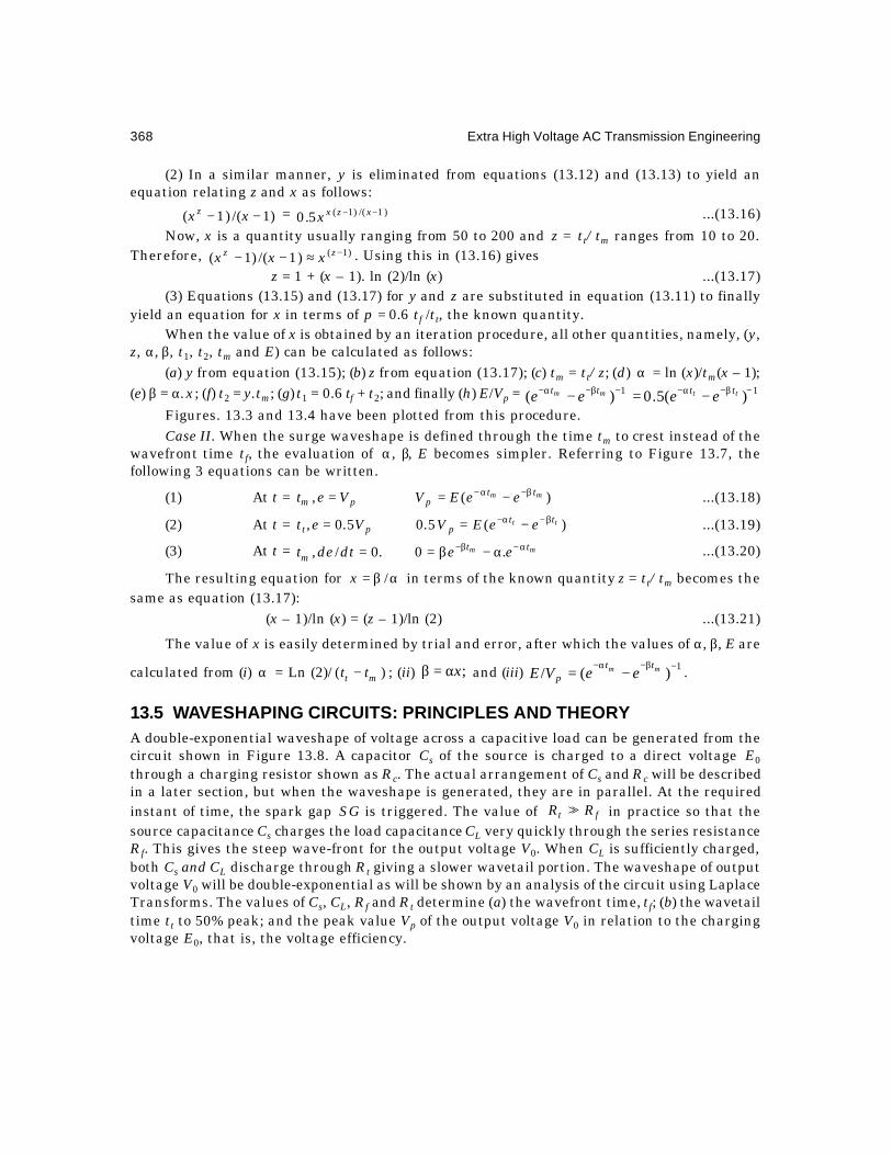
368 Extra High Voltage AC Transmission Engineering
(2) In a similar manner, y is eliminated from equations (13.12) and (13.13) to yield anequation relating z and x as follows:
)1/()1( −− xx z = )1/()1(5.0 −− xzxx ...(13.16)
Now, x is a quantity usually ranging from 50 to 200 and z = tt/tm ranges from 10 to 20.Therefore, )1()1/()1( −≈−− zz xxx . Using this in (13.16) gives
z = 1 + (x – 1). ln (2)/ln (x) ...(13.17)(3) Equations (13.15) and (13.17) for y and z are substituted in equation (13.11) to finally
yield an equation for x in terms of p = 0.6 tf /tt, the known quantity.When the value of x is obtained by an iteration procedure, all other quantities, namely, (y,
z, α, β, t1, t2, tm and E) can be calculated as follows:(a) y from equation (13.15); (b) z from equation (13.17); (c) tm = tt/z; (d) α = ln (x)/tm(x – 1);
(e) β = α. x ; (f) t2 = y.tm; (g) t1 = 0.6 tf + t2; and finally (h) E/Vp = 11 )(5.0)( −β−α−−β−α− −=− ttmm tttt eeeeFigures. 13.3 and 13.4 have been plotted from this procedure.Case II. When the surge waveshape is defined through the time tm to crest instead of the
wavefront time tf, the evaluation of α, β, E becomes simpler. Referring to Figure 13.7, thefollowing 3 equations can be written.
(1) At t = )(, mm ttppm eeEVVet β−α− −=∴= ...(13.18)
(2) At t = )(5.05.0, tt ttppt eeEVVet β−α− −=∴= ...(13.19)
(3) At t = mm ttm eedtdet α−β− α−β=∴= .0.0/, ...(13.20)
The resulting equation for αβ= /x in terms of the known quantity z = tt/tm becomes thesame as equation (13.17):
(x – 1)/ln (x) = (z – 1)/ln (2) ...(13.21)
The value of x is easily determined by trial and error, after which the values of α, β, E are
calculated from (i) α = Ln (2)/ )( mt tt − ; (ii) ;xα=β and (iii) 1)(/ −β−α−−= mm tt
p eeVE .
13.5 WAVESHAPING CIRCUITS: PRINCIPLES AND THEORYA double-exponential waveshape of voltage across a capacitive load can be generated from thecircuit shown in Figure 13.8. A capacitor Cs of the source is charged to a direct voltage E0
through a charging resistor shown as Rc. The actual arrangement of Cs and Rc will be describedin a later section, but when the waveshape is generated, they are in parallel. At the requiredinstant of time, the spark gap SG is triggered. The value of ft RR >> in practice so that thesource capacitance Cs charges the load capacitance CL very quickly through the series resistanceRf. This gives the steep wave-front for the output voltage V0. When CL is sufficiently charged,both Cs and CL discharge through Rt giving a slower wavetail portion. The waveshape of outputvoltage V0 will be double-exponential as will be shown by an analysis of the circuit using LaplaceTransforms. The values of Cs, CL, Rf and Rt determine (a) the wavefront time, tf; (b) the wavetailtime tt to 50% peak; and the peak value Vp of the output voltage V0 in relation to the chargingvoltage E0, that is, the voltage efficiency.

EHV Testing and Laboratory Equipment 369
Fig. 13.8 Equivalent circuit of an impulse voltage generator forcalculating waveshaping components.
The charging resistor Rc is extremely high and is in parallel with Cs so that its effect onthe waveshape of output voltage is negligible. However, we will retain Rc in deriving the equationsand then let ∞→cR . The operational form of the relation between the output voltage V0(s)and the charging voltage (E0/s) when the spark gap SG is conducting will be
V0(s) =
1
20 1111−
+++
++++
Lstfc
tfc
scLtLfsfLf CCRRR
RRRs
CRCRCRCRs
CRE
...(13.22)
Now, if the output voltage is )()(0tt eeEtV β−α− −= , its Laplace Transform is
V0(s) = ])(/[)( 2 αβ+β+α+α−β ssE ...(13.23)
Comparing (13.22) and (13.23), and equating coefficients of like powers of s, there resultthe required equations between the generator components and the values of α, β, E determinedfrom required timings as described in the previous section. These are:
scLtLfsf CRCRCRCR1111
+++ = β+α ...(13.24)
Lstfctfc CCRRRRRR /)( ++ = αβ ...(13.25)
and LfCR = α−β1
.0
EE
...(13.26)
There are 5 unknown parameters Rc, Rf, Rt, Cs, CL and only 3 equations. However, inpractice, the source capacitance and charging resistor are fixed when an impulse generator ispurchased and installed in a high-voltage laboratory. It is then necessary to choose propervalues of Rf and Rt for a given load capacitance CL. The values of E,,βα are taken from Figs.13.3 and 13.4 for the generation of required waveshapes for lightning and switching impulses.
When Rc is very large (> 1 Megohm), we obtain the following equations from (13.24) and(13.25):
LtLfsf CRCRCR111 ++ = αβ=β+α Lstf CCRR/1and, ...(13.27)
Solving these for Rf and Rt, there result
Rt =
β+α
+αβ−±
+αββ+α
2)(
)(411
)(2 L
Ls
Ls C
CCCC ...(13.28)
after whichRf = αβLst CCR/1 ...(13.29)
V0Rc Rt
Rf
CLCs
E0
SG
+
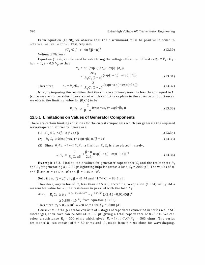
370 Extra High Voltage AC Transmission Engineering
From equation (13.28), we observe that the discriminant must be positive in order toobtain a real value for Rt. This requires
)/( sL CC ≥ 2)(4 α−βαβ ...(13.30)Voltage EfficiencyEquation (13.26) can be used for calculating the voltage efficiency defined as 0/ EVpv =η .
At t = tt, e = 0.5 Vp so thatVp = 2E (exp ))exp()( tt tt β−−α−
= ))exp()(exp()(
2 0tt
Lftt
CRE
β−−α−α−β ...(13.31)
Therefore, 0/EVpv =η = ))exp().(exp()(
2tt
Lf
ttCR
β−−α−α−β ...(13.32)
Now, by imposing the condition that the voltage efficiency must be less than or equal to 1,(since we are not considering overshoot which cannot take place in the absence of inductance),we obtain the limiting value for (RfCL) to be
LfCR ≥ ))exp()(exp(2
tt tt β−−α−α−β ...(13.33)
12.5.1 Limitations on Values of Generator ComponentsThere are certain limiting equations for the circuit components which can generate the requiredwaveshape and efficiency. These are
(1) αβα−β≤ 4/)(/ 2Ls CC ...(13.34)
(2) )/())exp()(exp(2 α−ββ−−α−≥ ttLf ttCR ...(13.35)
(3) Since tsLf RCCR αβ= /1 , a limit on Rt Cs is also placed, namely,
stCR =1))exp()(exp(
2
1 −β−−α−αβ
α−β≤
αβ ttLf
ttCR ...(13.36)
Example 13.3. Find suitable values for generator capacitance Cs and the resistances Rfand Rt for generating a 1.2/50 µs lightning impulse across a load CL = 2000 pF. The values of αand β are α = 14.5 × 10³ and β = 2.45 × 10⁶.
Solution. αβα−β 4/)( 2 = 41.74 and 41.74 CL = 83.5 nF.
Therefore, any value of Cs less than 83.5 nF, according to equation (13.34) will yield areasonable value for Rt, the resistance in parallel with the load CL.
Also, 65045.21050105.14 10)0145.045.2/()(263
−−≥ ×−×××− −eeCR Lf
,10398.0 6−×≥ from equation (13.35)
Therefore Rf 200102.0 3 =×≥ ohms for CL = 2000 pF.
Comments. If the generator consists of 6 stages of capacitors connected in series while SGdischarges, then each can be 500 nF = 0.5 µF giving a total capacitance of 83.3 nF. We canselect a resistance Rf = 300 ohms which gives fLst RCCR αβ= /1 = 563 ohms. The seriesresistance Rf can consist of 6 × 50 ohms and Rt made from 6 × 94 ohms for waveshaping.

EHV Testing and Laboratory Equipment 371
According to equation (13.32) the voltage efficiency falls to 66.3%. In order to increase theefficiency, a lower value of Rf can be used which will require a higher value for Rt. For example,with Rf = 250 ohms, the efficiency is increased to 83% and Rt = 680 ohms.
Example 13.4. The generator of previous example with Cs = 83.3 nF is required to generate
a switching impulse of approximately 250/2500 µs waveshape for which α = 365 and β = 11 ×103. Design the values of CL, Rf, Rt and find the efficiency.
Solution. 2)/(4 α−βαβ≥sLCC from equation (13.34). With given values, nF83.11≥LC .
We observe that the load capacitance is much higher for generating switching surge thanfor lightning impulse generation.
6105.75)/()exp(exp2 −×=α−ββ−−α−≥ ttLf ttCR
Therefore 6382≥fR ohms.Let CL = 12 nF and Rf = 6.4 kilohms. Then Rt = 39 k.
Voltage efficiency vη = 75.5 × 10⁻⁶/(6.4 × 103 × 12 × 10–9) = 98.3%.
13.5.2 Approximate Equations for Quick Estimation of Rf and Rt
The previous discussion used a rigorous method of determining the values of waveshapingresistors with given generator capacitance and required load capacitance. A quick butapproximate set of values for Rf and Rt can be obtained by the following procedure, on the linesof the following ideas.
(1) During the generation of the fast wavefront, the parallel resistance Rt has littleinfluence over charging the load capacitance CL from the generator capacitance Cg.
(2) Similarly, during the generation of the wavetail portion of the impulse, when bothcapacitances discharge through Rt, the series resistor exercises little influence.
Fig. 13.9 Equivalent circuits during formation of wavefront andwavetail for quick estimation of Rf and Rt.
These suggest the equivalent circuits Figure 13.9 (a) and (b) for the generation of wavefrontand wavetail.
For the circuit of 13.9 (a),
v0(t) = )/exp1(0f
Ls
s TtCC
CE−−
+ ...(13.37)
and for 13.9 (b),
)(0 tv = )/exp(.0t
Ls
s TtCC
CE−
+ ...(13.38)
V0
E0
Cs
Rf
CL
( )a
+
( )b
V0CLRtCs
E0+

372 Extra High Voltage AC Transmission Engineering
The two time constants Tf and Tt are, respectively,
Tf = fLsLsf RCCCCR =+ )/( × (Cs and CL in series) ...(13.39)and
Tt = ×=+ tLst RCCR )( (Cs and CL in parallel) ...(13.40)
When the front and tail timings tf and tt of the wave are specified, the values of Rf and Rtcan be calculated as shown below in terms of Cs and CL.
At t = t2, v0 = 0.3 giving 1 – exp (– t2/Tf) = 0.3, from Figure 13.7, andat t = t1, v0 = 0.9 giving 1 – exp (–t1/Tf) = 0.9.These yield t2 = 0.3567 Tf and t1 = 2.303 Tf.But by definition,
tf = 1.67 (t1 – t2) = )/(25.325.3 LsLsff CCCCRT += ...(13.41)
Therefore Rf = LsLsf CCCCt /).(3077.0 + . ...(13.42)
Again, from the definition of wavetail timing, exp (–tt/Tt) = 0.5 giving tt/Tt = ln 2 = 0.6931.Therefore Tt = tt/0.6931 = 1.4428 tt.
But, Rt = )/(4428.1)/( LstLst CCtCCT +=+ ...(13.43)Therefore, equations (13.42) and (13.43) give values for Rf and Rt very quickly when
fLs tCC ,, and tt are known and does not require a knowledge of α and β . However, theseresistance values are approximate and in a laboratory some adjustment will be necessary afterlooking at the actual waveform on an oscilloscope.
Example 13.5. With Cs = 83.3 nF, CL = 2nF for the lightning-impulse generator of example13.3 and tf = 1.2 µs, tt = 50 µs, calculate approximate values of Rf and Rt required and comparethem with the values in example 13.3.
Solution. From equation (13.42),Rf = 0.3077 × 1.2 × 10–6 × 85.3 × 10–9/166.6 × 10–18 = 189 ohms.
Note that Rf was calculated to have a minimum value of 200 ohms in the previous example.From equation (13.43)
Rt = 1.4428 × 50 × 10–6/85.3 × 10–9 = 846 ohms.From the exact expression Rt can be calculated for Rf = 200 ohms which will be
fLst RCCR αβ= /1 = 846 ohms. This is exactly the same value as obtained from the approximateequivalent circuit, Figure 13.9(b).
Example 13.6. Estimate the values of Rf and Rt quickly for the switching-surge generatorwith Cs = 83.3 nF, CL = 12 nF, tf = 250 µs, and tt = 2500 µs.
Solution. Rf = 0.3077 × 0.25 × 10–3 × 95.3 × 10–9/(83.3 × 12 × 10–18)= 7.33 kilohms.
The value obtained in example 13.4 was 6.4 kilohms.Rt = 1.4428 × 2.5 × 10–3/95.3 × 10–9
= 38 kilohms against 39 kilohms obtained before.From equation (13.37) and Figure 13.9 (a) we observe that Rf controls the wavefront time
and so is called the wavefront resistor. Similarly, Rt may be designated the wavetail resistor, asshown in equation (13.38) and Figure 13.9 (b).

EHV Testing and Laboratory Equipment 373
13.6 IMPULSE GENERATORS WITH INDUCTANCEIn section 13.5, the several inductances inherent in an impulse generator and the test circuitwere not considered. There exist inductances in the generator itself, the connecting leads, andmeasuring system which give rise to a deformation of the ideal double-exponential waveformon the front, peak, and tail. Thus, no waveshape generated in an impulse generator is trulydouble exponential . These inductances are
(a) inductance in the generator capacitance, resistors, and leads connecting theminternally;
(b) inductance in the high-voltage lead connecting the generator output terminal withthe voltage divider and the test object:
(c) inductance in the voltage divider column; and(d) inductance in the ground connection.
13.6.1 Inductance in GeneratorIn Figure 13.10(a) an inductance L is shown in series with Cs. In normal practical impulsegenerator circuits, the arrangement of Rf and Rt can change with the generator connection. Inthis circuit, Rt is shown on the source side but this does not alter the characteristics to anygreat extent from the previous section. The operational expression for the output voltage is
V0(s) =cbsassLCRR
RE
Ltf
t
++++ 2201
.)(
...(13.44)
+=
+++=
++=
Lstf
LstfstLtLf
LtfLtf
CLCRRc
CCLRRCRCRCRb
CLRRCRRLa
)/(1and
)/()(
,)/()(where
..(13.45)
Two cases arise for the roots of the denominator,s2 + as2 + bs + c = 0.
These are:
(1) All three roots are real. Let these be ),,( γ−β−α− . Then the time response of output
voltage will be
v0(t) = ])()()[())()((
1.
)(.0
ttt
Ltf
t eeeLCRR
RE γ−β−α− α−β+γ−α+β−γ
α−γγ−ββ−α+...(13.46)
(2) One real root α− , and a pair of complex conjugate roots γ±β− j . For this case, the
inverse transform of equation (13.44) is
v0(t) = )]sincos([)(0 tDtBeAeLCRR
RE tt
Ltf
t γ+γ++
β−α− ...(13.47)
αγαβ−γ+β−=
−=γ+α−β=
)/()(1and
,,)/(1where22
22
AD
ABA...(13.48)

374 Extra High Voltage AC Transmission Engineering
Fig. 13.10(a) Impulse generator with inductance. (b) Impulse voltage divider withresistance and inductance connected to impulse generator and load capacitance.
Example 13.7. For an impulse generator, take Cs = 20 nF, CL = 2 nF, Rf = 376 ohms, Rt
= 3120 ohms. For L = 40 µH and 100 µH, obtain the values of βα, and γ.Solution. Using Newton's method for finding the real root of a cubic equation, the following
values are obtained:
(a) L = .10688.6,1083.1,046,14:H40 66 ×=γ×=β=αµ
(b) L = .10363.1,10743.1,050,14:H100 66 ×=γ×=β=αµ
For the above generator, the behaviour of wavefront of the surge is calculated and shownin Figure 13.11 for the cases of L = 0, 40 µH, and 100 µH. The effect of increasing Rf to 550ohms is also shown on its lengthening of wavefront and reducing the voltage efficiency.
The inductance of e.h.v. impulse generators range from 3 to 4 µH per stage. A 12-stagegenerator has a total inductance of about 40 µH when all stages are connected in series duringdischarge.
Fig. 13.11 Effect of impulse-generator inductance onwavefront of lightning impulse.
V0CL
Rf
Rt
E0
Cs
L
( )a
+
V0
RfRd
Ld
Cd
Rt
E0
Cs
( )b
+
CL
314
1.0
0.8
0.6
0.4
0.2
0
2
VE
00
/
0 0.5 1.0 1.5 2.0 2.5t s, µ
1 = 0, = 376
2
L Rf = 40 H, = 376
3 = 100 H, = 376
4 = 40 H, = 550
L RL RL R
µµ
µ
f
f
f

EHV Testing and Laboratory Equipment 375
13.6.2 Inductance of Lead Connecting Generator and LoadThe physical sizes of extra high voltage equipment, laboratory dimensions and air gap clearancesare on the increase to that very long leads are necessary in order to interconnect variouscomponents during testing. These give rise to travelling-wave effects when the generatordischarges. For example, a lead length of 20 metres has a travel time for the impulse of 1/15thmicrosecond at light velocity. Repeated reflections from the generator and load give rise tooscillations which will appear on both the load and the measuring system. This affects thebuildup of the wavefront. This has been investigated intensively by manufacturers and testingengineers resulting in the invention of the Zaengel Voltage Divider measuring system. It usesa suitable value of resistor at the entrance to the voltage divider high-voltage terminal to dampthe oscillations.
13.6.3 Inductance of the Voltage DividerVoltage dividers are used for stepping down the high voltage to a value suitable for the low-voltage measuring equipment. These dividers may be of the pure resistive type, pure capacitivetype, or a combination of resistance and capacitance, the resistor used only to damp any naturaloscillation caused by the high-voltage capacitor and the inductance originating from the heightof the capacitor itself. For example, a capacitance of 1000 pF with an inductance of 2.5 µH
requires a resistance ddd CLR /2= = 100 ohms for critical damping of the oscillations. Theeffect of inductance Ld of the divider is to increase the rate of rise of wavefront so that themeasured waveform will have a shorter wavefront time than the actual voltage to which thetest object will be subjected.
The equivalent circuit of an impulse generator circuit considering the divider capacitance,inductance, and resistance is shown in Figure 13.10(b). The Laplace-Transform of the outputvoltage is
V0(s) =qpsnsmss
bassCR
E
Lf ++++++234
20 . ...(13.49)
++=
++++=
++++=
+++=
==
)/()(and
)/()(/)/1/1/1(
/1)/1/1/1)(/(/1
/1/1/1/
,/1,/where
22ddLstftfdst
ddLtffdddstsfLf
LstfstsfLfdddd
stsfLfdd
dddd
LCCCRRRRCCRq
LCCRRRRCLcRCRCRp
CCRRCRCRCRLRCLn
CRCRCRLRm
CLbLRa
...(13.50)
The inverse transform can be evaluated when numerical values for all circuit componentsare given. Figure 13.12 shown waveforms (with an expanded wavefront) for an impulse generatorwhose details are as follows:
Cs = 20.8 nF, CL = 1 nF, Rf = 276 ohms, Rt = 3120 ohms
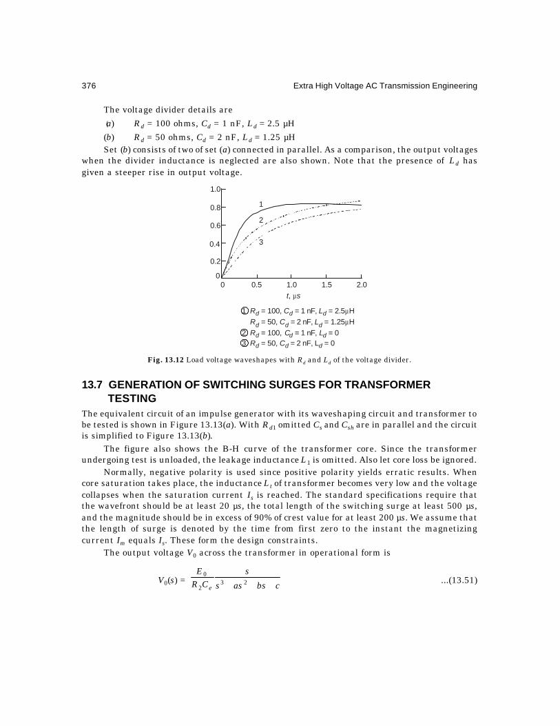
376 Extra High Voltage AC Transmission Engineering
The voltage divider details are
(a) Rd = 100 ohms, Cd = 1 nF, Ld = 2.5 µH
(b) Rd = 50 ohms, Cd = 2 nF, Ld = 1.25 µHSet (b) consists of two of set (a) connected in parallel. As a comparison, the output voltages
when the divider inductance is neglected are also shown. Note that the presence of Ld hasgiven a steeper rise in output voltage.
Fig. 13.12 Load voltage waveshapes with Rd and Ld of the voltage divider.
13.7 GENERATION OF SWITCHING SURGES FOR TRANSFORMERTESTING
The equivalent circuit of an impulse generator with its waveshaping circuit and transformer tobe tested is shown in Figure 13.13(a). With Rd1 omitted Cs and Csh are in parallel and the circuitis simplified to Figure 13.13(b).
The figure also shows the B-H curve of the transformer core. Since the transformerundergoing test is unloaded, the leakage inductance L1 is omitted. Also let core loss be ignored.
Normally, negative polarity is used since positive polarity yields erratic results. Whencore saturation takes place, the inductance Lt of transformer becomes very low and the voltagecollapses when the saturation current Is is reached. The standard specifications require thatthe wavefront should be at least 20 µs, the total length of the switching surge at least 500 µs,and the magnitude should be in excess of 90% of crest value for at least 200 µs. We assume thatthe length of surge is denoted by the time from first zero to the instant the magnetizingcurrent Im equals Is. These form the design constraints.
The output voltage V0 across the transformer in operational form is
V0(s) = cbsass
sCR
E
e +++ 232
0...(13.51)
1.0
0.8
0.6
0.4
0.2
00 0.5 1.0 1.5 2.0
t s, µ
1
2
3
1 = 100, = 1 nF, = 2.5 H
C Ld µRR C LR C LR C
d d
d d d
d d d
d d d
= 50, = 2 nF, = 1.25 H
2 = 100, = 1 nF, = 03 = 50, = 2 nF, L = 0
µ

EHV Testing and Laboratory Equipment 377
+=+=
++=
)/()(and
)/()(
)/()(where
2121
2121
21211
tes
tests
teseest
LCCRRRRcLCCRRLCRRb
LCCRRCRCRCRLa
...(13.52)
Fig. 13.13(a) Complete equivalent circuit of transformer undergoing switching impulse test.(b) Simplified equivalent circuit.(c) B-H curve of transformer core illustrating saturation current.
Let the roots of the polynomial (s3 + as2 + bs + c) = 0 be denoted as s = – p, – q + jr,– q – jr. Then, the time variation of the output voltage will be
V0(t) = )]cos(.[ .22
2
0 ϕ−++ −− rteCBAeCR
E qtpt
e...(13.53)
+−−+=
+−−=−=
])(/[)(
)/(where2222
22
rpqrpqrqC
rpqpBA...(13.54)
and tan ϕ = C/B.The current through the magnetizing inductance is
Im(s) = V0(s)/sLt ...(13.55)
( )a
Generator Wave-ShapingCircuit
Transformer
+E0
Cs
Rd1 Rd2 R1 L1 L1 R1
CteLtRtCshRc
S G
V0LtCe
R2
R1
E0
Cs
( )b
+Im
Is
V
( )c
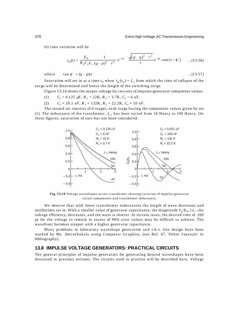
378 Extra High Voltage AC Transmission Engineering
Its time variation will be
im(t) =
ϕ−
+++
+−−− )cos(.
)(
)(
1 22
222
0 'rter
rqpe
rpqLCRE qtpt
te...(13.56)
where 'ϕtan = (q – p)/r ...(13.57)
Saturation will set in at a time t0 when Itim =)( 0 s, from which the time of collapse of thesurge will be determined and hence the length of the switching surge.
Figure 13.14 shows the output voltage for two sets of impulse-generator component values.
(1) Cs = 0.125 µF, R1 = 22K, R2 = 3.7K, Ce = 6 nF.
(2) Cs = 20.1 nF, R1 = 132K, R2 = 22.2K, Ce = 10 nF.The second set consists of 6 stages, each stage having the component values given by set
(1). The inductance of the transformer, Lt, has been varied from 10 Henry to 100 Henry. Onthese figures, saturation of core has not been considered.
Fig. 13.14 Voltage waveshapes across transformer showing variation of impulse-generatorcircuit components and transformer inductance.
We observe that with lower transformer inductances the length of wave decreases andoscillations set in. With a smaller value of generator capacitance, the magnitude Vp/E0, i.e., thevoltage efficiency, decreases, and the wave is shorter. In certain cases, the desired time of 200µs for the voltage to remain in excess of 90% crest values may be difficult to achieve. Thewavefront becomes steeper with a higher generator capacitance.
Many problems in laboratory waveshape generation and e.h.v. line design have beenworked by Ms. Amruthakala using Computer Graphics, (see Ref. 47, 'Other Journals' inbibliography).
13.8 IMPULSE VOLTAGE GENERATORS: PRACTICAL CIRCUITSThe general principles of impulse generators for generating desired waveshapes have beendiscussed in previous sections. The circuits used in practice will be described here. Voltage
– 0.4
– 0.2
0
0.2
0.4
0.6
0.8
1.0 1.0
0.8
0.6
0.4
0.2
0
– 0.2
– 0.4
121 23
10
5050
10
100100
3t, ms
LT, HenryLT, Henry
VE
00
/Cs = 0.021 FµCs = 0.125 FµCL = 100 nFCL = 6 nF
R1 = 132 KR1 = 22 K
R2 = 22.2 KR2 = 3.7 K
t, ms

EHV Testing and Laboratory Equipment 379
dividers used for measuring the high voltages as well as voltmeters, oscilloscopes, and otherequipment will be described in the next section.
The important components of an impulse generator are basically (a) the impulse capacitor,Cs; (b) the load capacitor CL; (c) the wavefront-shaping resistor, Rf; and (d) the wavetail-shapingresistor, Rt. In addition, other components are the charging transformer-rectifier, the chargingresistor, spark gaps and other auxiliaries. In some generators, the series resistor Rf is insertedbetween the high-voltage output terminal and the terminal common to the voltage divider andtest object. In other designs, it consists of several smaller resistors connected in series with theimpulse capacitors in each stage in order to damp out any oscillations occurring due to stageinductance. In principle, the generation of extremely high voltages up to 6000 kV or 6 MVrequires a very large number of stages of capacitors, each rated for about 200 kV, to be chargedin parallel from the low voltage, and discharged in series.
Figure 13.15 shows a complete schematic diagram of one type of Marx Circuit. Figure13.16 shows the overall equivalent circuit when discharging. Only 4 stages are shown for claritybut this could be extended to any number, say 30, built on the same principle.
Fig. 13.15 Practical 4-stage impulse generator circuit layout.
Referring to Figure 13.15, 50 Hz ac is supplied to the regulating transformer (1) throughan isolating transformer (not shown). The isolating transformer is usually a 3-phase transformerat power-frequency voltage with only two of the three windings used on the secondary side.Thus, line-to-line voltage is fed to the regulating winding (1). The diode (3) delivers a rectified
109
7
4321
6
8
5
Rc
Rc
Rc
Rp
Cg
Rs
Rse
TestObject
VoltageDividerH.V.Arm
L.V.Arm
SGD
ImpulseGround
A.C.50 Hz

380 Extra High Voltage AC Transmission Engineering
ac to charge the impulse-generator capacitance Cg. While the first or lowest stage is chargeddirectly, the second and subsequent-stage capacitances are charged through a combination ofRc, Rs, and Rp. The higher stages therefore acquire charges at slower rates but the final voltageof all stages will be the same. The spark gaps SG are set such that they do not sparkover at thevoltage used during charging.
Fig. 13.16 Equivalent circuit of generator when discharging.
After all the stages have acquired their final voltage, the test engineer can 'fire' theimpulse generator by applying a suitable potential to the lowest spark gap (7). If the stagevoltage is Es, then breakdown of the first gap places two capacitors in series, assuming thevalue of Rc to be very high, as shown in Figure 13.17. The voltage across the spark gap SG2 isnow high enough to cause it to breakdown. The successive sparkover of all gaps places theseveral stages of capacitors in series to that the output voltage at the high-voltage terminal toground is nearly nEs. The test object is now impulsed. The voltage divider is used for supplyinga suitable low voltage to the measuring system consisting of (a) a high-voltage high writing-speed oscilloscope, (b) a peak voltmeter, or (c) a digital reading device of the voltage.
Fig. 13.17 Conditions during firing of series spark gap.
An arrangement for initiating the triggering of the lowest gap is variously known as a 3-electrode arrangement or a trigatron. Figure 13.18 shows a simplified diagram of thearrangement. A low-voltage impulse generator discharges through a coupling capacitor to athird electrode called the Triggering Electrode which will place a voltage of opposite polarity to
SG
V.D.
Rf
CLRt
E0
Cs
Cg/n
+
Rc
Es
Rs
Rp
Cg
SG2
Es
+
+
34
RpRc
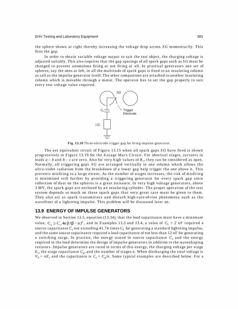
EHV Testing and Laboratory Equipment 381
the sphere shown at right thereby increasing the voltage drop across SG momentarily. Thisfires the gap.
In order to obtain variable voltage output to suit the test object, the charging voltage isadjusted suitably. This also requires that the gap spacings of all spark gaps such as SG must bechanged to prevent anomalous firing or not firing at all. In practical generators one set ofspheres, say the ones at left, in all the multitude of spark gaps is fixed to an insulating columnas tall as the impulse generator itself. The other companions are attached to another insulatingcolumn which is movable through a motor. The operator has to set the gap properly to suitevery test voltage value required.
Fig. 13.18 Three-electrode trigger gap for firing impulse generator.
The net equivalent circuit of Figure 13.15 when all spark gaps SG have fired is shownprogressively in Figure 13.19 for the 4-stage Marx Circuit. For identical stages, currents inleads a – b and b – c are zero. Also for very high values of Rc, they can be considered as open.Normally, all triggering gaps SG are arranged vertically in one column which allows theultra-violet radiation from the breakdown of a lower gap help trigger the one above it. Thisprevents misfiring to a large extent. As the number of stages increases, the risk of misfiringis minimized still further by providing a triggering generator for every spark gap sincecollection of dust on the spheres is a great nuisance. In very high voltage generators, above3 MV, the spark gaps are enclosed by an insulating cylinder. The proper operation of the testsystem depends so much on these spark gaps that very great care must be given to them.They also act as spark transmitters and disturb high-rate-of-rise phenomena such as thewavefront of a lightning impulse. This problem will be discussed later on.
13.9 ENERGY OF IMPULSE GENERATORSWe observed in Section 13.5, equation (13.34), that the load capacitance must have a minimumvalue, 2)/(4. α−βαβ≥ sL CC , and in Examples 13.3 and 13.4, a value of CL = 2 nF required asource capacitance Cs not exceeding 41.74 times CL for generating a standard lightning impulse,and the same source capacitance required a load capacitance of not less than 12 nF for generatinga switching surge. In practice, the energy stored in source capacitance Cs and the energyrequired in the load determine the design of impulse generators in addition to the waveshapingresistors. Impulse generators are rated in terms of this energy, the charging voltage per stageEs, the stage capacitance Cg, and the number of stages n. When discharging the total voltage isV0 = nEs and the capacitance is Cs = Cg/n. Some typical examples are described below. For a
SG
I.G.
Cs TriggerElectrode

382 Extra High Voltage AC Transmission Engineering
given stage capacitance Cg and charging voltage Es, the energy increases n times when thecapacitors are re-connected in n stages instead of 1 stage. For example, let the capacitance in 1stage equal 125 nF = 0.125 µF, and the charging voltage 200 kV. The energy stored is
250021 2 =cV J = 2.5 kJ. If the capacitors are connected in 4 stages in order to test an object at
higher voltage, the total capacitance reduces to 125/4 = 31.25 nF. But when all stages dischargein series and the charging voltage per stage is still 200 kV, the total energy delivered by the
generator is 239 )10800(1025.3121
×××× − = 10.0 kJ.
Fig. 13.19. Equivalent circuit for Fig. 13.15.
The choice of total energy in the generator, the stage capacitance and voltage will begoverned by the tests to be carried out and the characteristics of the test object. Impulsegenerators for testing line equipment only such as insulators, air-core transformers, etc., willneed low energies while those that test long cables and high-voltage transformers will needcorrespondingly higher energies. The following table gives typical energies and capacitance inn stages in series required when the stage voltages are taken to be 100 kV and 200 kV. Thecapacitances are given in nF.
Rse Rse Rse
Rp Rp Rp
Rp Rp Rp
Rp Rp Rp
Rp
Rse
RtnRp
E0
Cs
= Cg /n
Rp Rp
Rs Rs
Rs Rs
Rs RsRs
Rs
Rs
Rs
Cg
Cg Cg
Cg
Cg
Cg
Cg
Cg
Cg
Cg
Cg
Rc
RcRc
RcRc
Rc
SG
Cg
a b c
To Load
V0CL
( – 1)n Rs

EHV Testing and Laboratory Equipment 383
Table: Total Capacitance of Impulse Generators when Discharging (nF)
Total Stage Voltage 100 kV Stage Voltage 200 kVEnergy, KJ n = 1 n = 10 n = 1 n = 10
2.5 500 5 125 1.255 1000 10 250 2.5
10 2000 20 500 520 4000 40 1000 1030 6000 60 1500 15
The relation between energy, stage voltage, number of stages in series when dischargingand total capacitance of generator when discharging is given by
KJ = 62 10).(21 −×× ss EnC ...(13.58)
where Cs = capacitance of generator in nF and Es = stage voltage in kV.
Example 13.8. An impulse generator consists of 6 stages with each stage having acapacitance of 0.125 µF (125 nF). The charging voltage is 200 kV. Calculate (a) the energyoutput of generator when all stages are connected in series, and (b) the energy when the 6capacitors are reconnected in 3 stages and the charging voltage per stage is kept the same as200 kV.
Solution. The two circuits are shown in Figure 13.20.
(a) Total generator capacitance when discharging = 12561 × = 20.83 nF.
Total voltage when discharging = 6 × 200 = 1200 kV.
Therefore, energy = 629 1012001083.2021
×××× −
= 15,000 Joules = 15 kJ.(b) When the generator is reconnected in 3 stages, each stage consists of 2 capacitors in
parallel, Figure 13.20(b), with a total stage capacitance of 250 nF. When the 3 stages dischargein series, the total generator capacitance is 250/3 = 83.3 nF, and the output voltage is 600 kV.
Therefore, energy = 629 10600103.8321
×××× −
= 15,000 Joules = 15 kJ.Equation 13.58 can also be used for the two cases.The capacitances of typical loads on an impulse generator may be summarized as follows:
Type of Test Object Capacitance Range, CL
(1) Line Insulators 50 pF for each disc. Total capacitance ofstring does not exceed a few pF.
(2) Bushings of Apparatus 100 to 500 pF(3) Power Transformers 1000 pF up to 1000 kVA
1000–10,000 pF over 1000 kVA(4) Cables 150 to 300 pF per metre length.
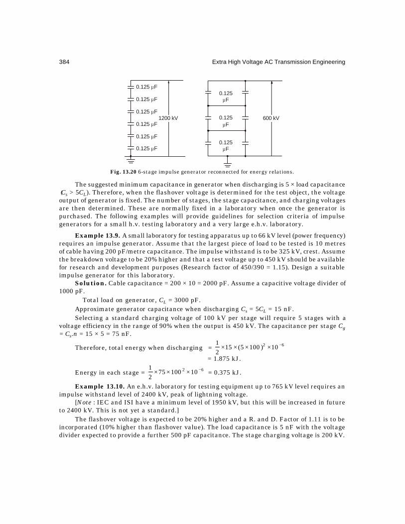
384 Extra High Voltage AC Transmission Engineering
Fig. 13.20 6-stage impulse generator reconnected for energy relations.
The suggested minimum capacitance in generator when discharging is 5 × load capacitance(Cs > 5CL). Therefore, when the flashover voltage is determined for the test object, the voltageoutput of generator is fixed. The number of stages, the stage capacitance, and charging voltagesare then determined. These are normally fixed in a laboratory when once the generator ispurchased. The following examples will provide guidelines for selection criteria of impulsegenerators for a small h.v. testing laboratory and a very large e.h.v. laboratory.
Example 13.9. A small laboratory for testing apparatus up to 66 kV level (power frequency)requires an impulse generator. Assume that the largest piece of load to be tested is 10 metresof cable having 200 pF/metre capacitance. The impulse withstand is to be 325 kV, crest. Assumethe breakdown voltage to be 20% higher and that a test voltage up to 450 kV should be availablefor research and development purposes (Research factor of 450/390 = 1.15). Design a suitableimpulse generator for this laboratory.
Solution. Cable capacitance = 200 × 10 = 2000 pF. Assume a capacitive voltage divider of1000 pF.
∴ Total load on generator, CL = 3000 pF.Approximate generator capacitance when discharging Cs = 5CL = 15 nF.Selecting a standard charging voltage of 100 kV per stage will require 5 stages with a
voltage efficiency in the range of 90% when the output is 450 kV. The capacitance per stage Cg= Cs.n = 15 × 5 = 75 nF.
Therefore, total energy when discharging = 62 10)1005(1521 −××××
= 1.875 kJ.
Energy in each stage = 62 101007521 −××× = 0.375 kJ.
Example 13.10. An e.h.v. laboratory for testing equipment up to 765 kV level requires animpulse withstand level of 2400 kV, peak of lightning voltage.
[Note : IEC and ISI have a minimum level of 1950 kV, but this will be increased in futureto 2400 kV. This is not yet a standard.]
The flashover voltage is expected to be 20% higher and a R. and D. Factor of 1.11 is to beincorporated (10% higher than flashover value). The load capacitance is 5 nF with the voltagedivider expected to provide a further 500 pF capacitance. The stage charging voltage is 200 kV.
0.125 Fµ
0.125 Fµ
0.125 Fµ
0.125 Fµ
0.125 Fµ
0.125 Fµ
1200 kV
0.125Fµ
0.125Fµ
0.125Fµ
600 kV

EHV Testing and Laboratory Equipment 385
Select the required stage capacitance, number of stages, and the energy of generatorwhen discharging.
Solution. The highest voltage required across the high voltage terminal of the generatoris 2400 × 1.2 × 1.11 = 3200 kV.
A voltage efficiency of 80% requires a total of 4000 kV in charging. Therefore, number ofstages = 4000/200 = 20. The load capacitance is CL = 5 + 0.5 = 5.5 nF. Hence, the generatorcapacitance when all 20 stages are discharging in series can be selected as Cs = 5CL = 27.5 nF.Therefore, the capacitance of each stage is Cg = 20 × 27.5 = 550 nF = 0.55 µF.
Energy = 62 10)20020(5.2721 −×××× = 220 kJ
Energy per stage = 62 1020055021 −××× = 11 kJ
[Note. For such large energies and high voltages, a manufacturer's catalogue must beconsulted for nearest standard size of capacitor, energy, and voltage efficiency.]
13.10 GENERATION OF IMPULSE CURRENTSLightning impulse currents up to 200,000 Amperes crest are generated by charging a set ofimpulse capacitors in parallel and discharging them the same way in a test object, which isusually a surge diverter or high rupturing-capacity fuse. The waveshape has a time to crest of8 µs, and 20 µs to 50% value on tail, as shown in Figure 13.2 before. Figure 13.21(a) shows theactual connection diagram and 13.21(b) the electrical equivalent circuit when the capacitorsare discharging through the test object.
Fig. 13.21 Impulse current generator:(a) Actual Schematic of Component Layout.(b) Equivalent Circuit.
A.C.50 Hz
CurrentShunt
ToScope
TestObject
( )a
C'1
C'1C'1
C'1
+ +
+
+
+
D TG
Va
IaIpE0
Ci
IG L R
( )b
8 20
+
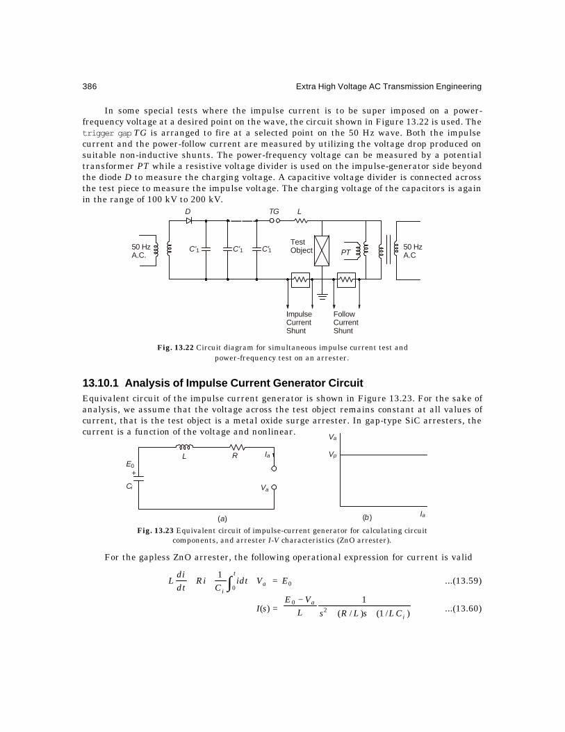
386 Extra High Voltage AC Transmission Engineering
In some special tests where the impulse current is to be super imposed on a power-frequency voltage at a desired point on the wave, the circuit shown in Figure 13.22 is used. Thetrigger gap TG is arranged to fire at a selected point on the 50 Hz wave. Both the impulsecurrent and the power-follow current are measured by utilizing the voltage drop produced onsuitable non-inductive shunts. The power-frequency voltage can be measured by a potentialtransformer PT while a resistive voltage divider is used on the impulse-generator side beyondthe diode D to measure the charging voltage. A capacitive voltage divider is connected acrossthe test piece to measure the impulse voltage. The charging voltage of the capacitors is againin the range of 100 kV to 200 kV.
Fig. 13.22 Circuit diagram for simultaneous impulse current test andpower-frequency test on an arrester.
13.10.1 Analysis of Impulse Current Generator CircuitEquivalent circuit of the impulse current generator is shown in Figure 13.23. For the sake ofanalysis, we assume that the voltage across the test object remains constant at all values ofcurrent, that is the test object is a metal oxide surge arrester. In gap-type SiC arresters, thecurrent is a function of the voltage and nonlinear.
Fig. 13.23 Equivalent circuit of impulse-current generator for calculating circuitcomponents, and arrester I-V characteristics (ZnO arrester).
For the gapless ZnO arrester, the following operational expression for current is valid
∫ +++t
ai
VidtC
Ridtdi
L0
1 = E0 ...(13.59)
I(s) = )/1()/(
12
0
i
a
CLsLRsLVE
++−
...(13.60)
C'1 C'1 C'1TestObject PT
50 HzA.C
50 HzA.C.
ImpulseCurrentShunt
FollowCurrentShunt
D LTG
E0
Ci Va
IaRL
+
( )a ( )b
Va
Vp
Ia

EHV Testing and Laboratory Equipment 387
The requirement of the generator is to develop a unidirectional current with a peak valueIp occurring at time tm and falling to 50% peak value at time tt. For the sake of preliminaryestimate, let us assume that the value of circuit resistance R can be adjusted to give criticaldamping of the circuit. Then,
R = iCL /2 . For this case,
I(s) = 20
)(
1
asLVE a
+
−...(13.61)
where a = R/2L. Also, R2/L2 = 4/LCi. ...(13.62)The, time variation of current through arrester is
i(t) = ata etL
VE −−..0 ...(13.63)
Its peak occurs when tm = 1/a = 2L/R. Therefore, atm = 1 ...(13.64)This is obtained by differentiating (13.63) with respect to t and letting di/dt = 0 to find tm.
Since tm = 8µs, there results R = 2L/tm ...(13.65)Therefore, the required value of R is obtained in terms of the circuit inductance L, and
known value of crest time tm.The peak value of current is
Ip = LCVEet
LVEet
LVE ia
maatm
ma .
73.2.... 0100 −=−=− −−
...(13.66)
At t = pt Itit 5.0)(, =
Therefore, tatt
a etL
VE −−..0 = a
tLaVE
ma 1
since,73.2
.5.0 0 =−...(13.67)
This gives a73.25.0
= tatt et −.
or tate = 2 atte ...(13.68)
This yields tat = )2ln( eatt ...(13.69)
or, with a = 1/tm,
)/ln(/ mtmt tttt − = 1.693 ...(13.70)
This equation determines the time tt to half value when crest time tm is known and for thecircuit critically damped.
Example 13.11. An R-L-C circuit is critically damped. It generates a current of the typei(t) = J.t. e–at with peak occurring at tm = 8 µs. (a) Calculate the time to 50% value on tail. (b) Ifthe circuit inductance is L = 40 µH, find the values of circuit resistance R and the capacitanceCi of the impulse capacitance when discharging.
Solution. (a) From equation (13.70), a trial and error solution givestt/tm = 2.68. ∴ tt = 2.68 × 8 = 21.44 µs.
This is nearly equal to the standard 20 µs. Therefore, the resistance is correct.

388 Extra High Voltage AC Transmission Engineering
(b) R = 2L/tm = 2 × 40 × 10–6/8 × 10–6 = 10 ohms.Ct = 4L/R2 = 1.6 µF.
If the damping is insufficient, the inverse transform of equation (13.60) should be workedout but with CLR /2> which gives two real roots for the polynomial in the denominator. Letthe waveshape be assumed a double exponential. Then
I(s) =
β+
−+α−β
−sasL
VE a 1110...(13.71)
−+=
−+=β
−−=
−−=α
ii
ii
LCaaCRLL
R
LCaaCRLL
R
22
22
/111/4112
and
/111/4112
where
...(13.72)
Also, α−β = ii LCaaCRLLR 22 /112/41 −=− ...(13.73)
Therefore
i(t) = ).()(]/41[
02/120 tttt
i
a eeIeeCRLR
VE β−α−β−α− −=−−
−...(13.74)
Referring to equation (13.21) in Section (13.4) where αβ= /x and mt ttz /= ,
(x – 1)/ln (x) = 2ln1)/(
)2ln(1
)/ln(1)/( −
=−
=αβ−αβ mt ttz
,
α = 10 )(/and,.),/()2ln( −β−α− −=α=β− mm tt
pmt eeIIxttThere are now sufficient equations for calculating R, Ct, and L when one of them is known.
Example 13.12. An impulse current generator consists of 10 impulse capacitors each of0.125 µF connected in parallel. The desired output waveshape has tm = 8 µs and tt = 20 µs.Calculate
(a) the approximate values of resistance and allowable inductance in the circuit to generatea double-exponential waveshape of current,
(b) the charging voltage to obtain peak value of Ip = 10 kA through an arrester whoseresidual voltage is 25 kV (3 p.u. on 6 kV, r.m.s, 8.486 kV, peak, base).
Solution. Let x = αβ / . Also, 5.28/20/ ==mt tt . Therefore
(x – 1)/ln (x) = (2.5 – 1)/ln 2 = 2.1642.A trial and error solution yields x = 4.
α = 410776.5)/(2ln ×=− mt tt , so that 4101.234 ×=α=β .
From equation (13.72)
5.776 × 104 = iLCaa 2/111( −−
and 23.1 × 104 = tLCaa 2/111( −+
This yields, a =R/2L = 14.44 × 10⁴, and LCi = 0.75 × 10⁻¹⁰.
EHV Testing and Laboratory Equipment 389
The given value of Ci = 10 × 0.125 µF = 1.25 × 10⁻⁶ Farad.Therefore L = 60 µH and hence R = 17.33 ohms.
From equation (13.74), I0 = kA.4.10
3486.8
/11
0
2
0 ×−=
−
− E
LCaR
VE
i
a
Therefore
Ip = )(4.10
47.25kA10
264 1081.2310810776.50 −− ××−×××− −−= eeE
giving E0 = 245.5 kV.The charging voltage is therefore about 250 kV. By increasing the source capacitance Ci
the charging voltage can be decreased. Note that in such high-current circuits, the voltageefficiency is not a factor of considerable importance.
13.11 GENERATION OF HIGH ALTERNATING TEST VOLTAGEPower frequency voltages up to 2000 kV, r.m.s., and 1A may be required for testing insulationstructures at e.h.v. levels. The short-duration test voltage required is 1.5 × highest equipmentvoltage (l – l) so that 1150 kV is required for 765 kV level. The flashover voltage is usually 20%higher and with a research and development factor of 1.1, there arises a need for a voltage of1520 kV in such a laboratory. For 1150 kV transmission equipment, based on a maximum of1200 kV, a power-frequency testing voltage of about 2000 kV may be required. Such highvoltages at low current levels are generated by cascade-connected units where more than 1transformer is connected in series. For example, at the IREQ laboratories in Canada, 4 units of600 kV are connected in series and the lower 2 units have two units in parallel making up atotal of 6 transformer. The need for the paralleling of the lower units arises for pollutiontesting of insulators to give a higher current (up to a voltage of 1200 kV) and lower leakagereactance. Normally, at these high voltages, except for insulator tests carried out under pollutedcondition, the load on a testing transformer is predominantly if not entirely capacitive. Thepower output of the transformer in MVA is
P = wC.V 2 × 10⁻⁶, MVA ...(13.75)where w = 2πf, C = load capacitance in µF, and V = test voltage at the high-voltage terminal
of transformer in kV, r.m.s.If the load capacitance is measured in pF, and the transformer power in kVA, then
P = wC V 2 × 10⁻⁹, kVA (C in pF, V in kV)When wet tests are carried out, there must be a reserve of power over that given above
because of leakage currents on the test piece. The load capacitance includes the capacitance ofthe test object, that of the transformer itself, and the large high-voltage shields and electrodesthat are necessary.
Typical ratings of single units might be as follows:
High Voltage Output Current Range (continuous) kVA Range
50 kV 40 mA to 400 mA 2 to 20100 100 mA to 500 mA 10 to 50200 0.5A to 2A 100 to 400350 0.5A to 2A 175 to 700600 1A to 3A 600 to 1800
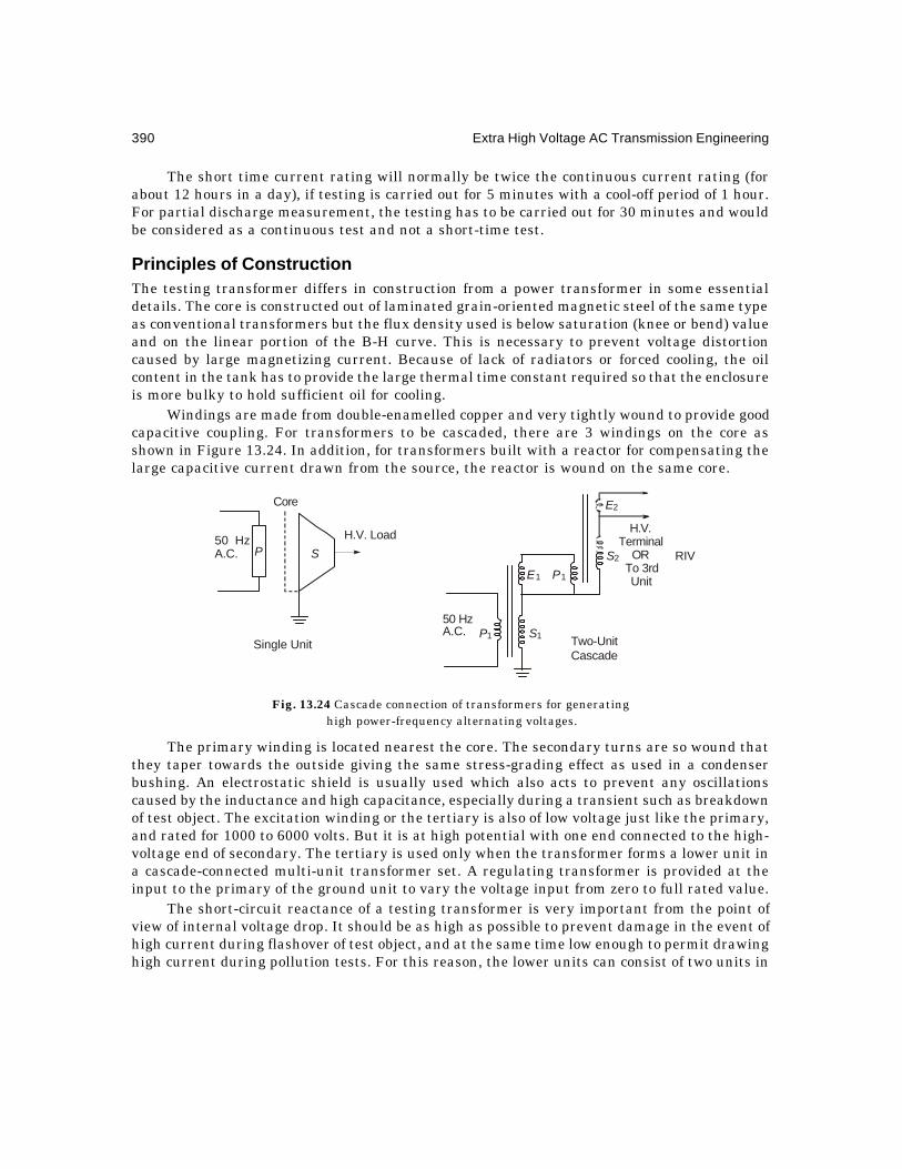
390 Extra High Voltage AC Transmission Engineering
The short time current rating will normally be twice the continuous current rating (forabout 12 hours in a day), if testing is carried out for 5 minutes with a cool-off period of 1 hour.For partial discharge measurement, the testing has to be carried out for 30 minutes and wouldbe considered as a continuous test and not a short-time test.
Principles of ConstructionThe testing transformer differs in construction from a power transformer in some essentialdetails. The core is constructed out of laminated grain-oriented magnetic steel of the same typeas conventional transformers but the flux density used is below saturation (knee or bend) valueand on the linear portion of the B-H curve. This is necessary to prevent voltage distortioncaused by large magnetizing current. Because of lack of radiators or forced cooling, the oilcontent in the tank has to provide the large thermal time constant required so that the enclosureis more bulky to hold sufficient oil for cooling.
Windings are made from double-enamelled copper and very tightly wound to provide goodcapacitive coupling. For transformers to be cascaded, there are 3 windings on the core asshown in Figure 13.24. In addition, for transformers built with a reactor for compensating thelarge capacitive current drawn from the source, the reactor is wound on the same core.
Fig. 13.24 Cascade connection of transformers for generating high power-frequency alternating voltages.
The primary winding is located nearest the core. The secondary turns are so wound thatthey taper towards the outside giving the same stress-grading effect as used in a condenserbushing. An electrostatic shield is usually used which also acts to prevent any oscillationscaused by the inductance and high capacitance, especially during a transient such as breakdownof test object. The excitation winding or the tertiary is also of low voltage just like the primary,and rated for 1000 to 6000 volts. But it is at high potential with one end connected to the high-voltage end of secondary. The tertiary is used only when the transformer forms a lower unit ina cascade-connected multi-unit transformer set. A regulating transformer is provided at theinput to the primary of the ground unit to vary the voltage input from zero to full rated value.
The short-circuit reactance of a testing transformer is very important from the point ofview of internal voltage drop. It should be as high as possible to prevent damage in the event ofhigh current during flashover of test object, and at the same time low enough to permit drawinghigh current during pollution tests. For this reason, the lower units can consist of two units in
E2
E1 P1
S1P1
S2
H.V.Terminal
ORTo 3rdUnit
RIV
Two-UnitCascade
50 HzA.C.
H.V. Load
S50 HzA.C.
Core
Single Unit
P

EHV Testing and Laboratory Equipment 391
parallel. Typical values of short-circuit voltage at rated current range from 1.5% to 40% ofrated value, the higher values applying for units in cascade. Single units may have up to about10% internal impedance but standard specifications must be consulted for the maximum allowed.When two units are paralleled, it drops to 5% for pollution tests.
Reactive CompensationWhen transformer windings, capacitors, and cables are tested, the load on the testing transformeris purely capacitive of a large magnitude. A testing transformer normally works at zero powerfactor leading in contrast to a power transformer whose power factor is almost always laggingand may be 0.9 or higher. Therefore, compensating reactors are necessary to minimize thetotal current drawn from the source in laboratories. The reactors can be externally connectedwith arrangements to switch them at predetermined levels of input current. This can only bedone in steps. An alternative is to build them on the same core as the transformer and connectthem in parallel with the primary windings in each unit. It is usual to provide a maximumcompensation at rated voltage amounting to 50% of the rated continuous power of the testingtransformer.
When the voltage of the transformer varies, the reactive power supplied by the built-inreactors also varies but as the square of the voltage in a parabolic manner. Figure 13.25 showsthe compensation provided as a function of voltage variation. Therefore, should extracompensation be necessary, external switched reactors have to be provided across the sourceto the ground unit. This is always single phase.
Fig. 13.25 Reactive compensation available with internally-built compensating reactors.
High Voltage Electrodes, Insulating Supports and EnclosuresBecause of the extremely high voltage used at the high voltage terminal, very large electrodesare necessary. The diameter of a nearly hemispherical electrode varies from 3 metres for a 300kV to 400 kV terminal to 5 metres for 2000 kV units. The minimum clearances required forsafety from the transformer range from 1.5 metres for 300 kV to almost 15 m for 2000 kV.Because of the large size of aluminium electrode required, it can be made in segments using anetwork of saucer-shaped electrodes each about 25 cm diameter. Such a construction has apatented name called POLYCON in Sweden.
100
75
50
25
012.5
%
Rated Power O
utput
Reactive Powerof Built-in Reactor
0 50 100

392 Extra High Voltage AC Transmission Engineering
Testing transformers have insulating cylinders made from reinforced fibre-glass or otherinsulating materials of high mechanical strength. The entire tank with oil, core, and windingsis placed inside this cylinder. This eliminates separate insulating pedestals necessary in cascade-connected transformers where the higher units must be insulated from ground for the voltageof the lower unit. There are several schemes for lowering this insulation requirement such asconnecting the high voltage secondary middle to the core, but these are details best discussedwith the manufacturers. However, a transformer using an insulated cylinder is only meant forindoor laboratory with a roof and walls to keep the elements out. For outdoor use, whicheliminates the need for a large building and its attendant costs, conventional steel tanks withporcelain bushings are necessary. Figure 13.26 shows the two constructions.
Fig. 13.26 Overall pictorial representation of cascade-connected transformers withinsulating cylinders and steel tanks.
A circuit diagram typical of a 2-unit cascade testing transformer installation is shown inFigure 13.27, together with source, regulating transformer, voltage divider and peak and r.m.s.voltmeters. One can also observe that with a 3-unit cascade-connected unit, it is possible to usethem as 3 separate single-phase units and perform experiments in 3-phase configuration at therated voltage of each unit. However, a suitable 3-phase source of supply is necessary for suchan eventuality. This facility is used when conducting high-voltage measurements on 3-phasetest lines to obtain corona loss values and such other properties as radio interference, electrostaticfields, and audible noise in 3-phase configuration, if single-phase test results are found inadequateto extrapolate to 3-phase results. Chapters 5 and 6 have covered the topic of conversion ofsingle-phase results to 3-phase lines and may be used in order to reduce the cost involved instringing a 3-phase line.
H.V. Electrode
BushingH.V.Load
TankIn
sula
ting
Col
umns
( )b( )a
50 HzSource
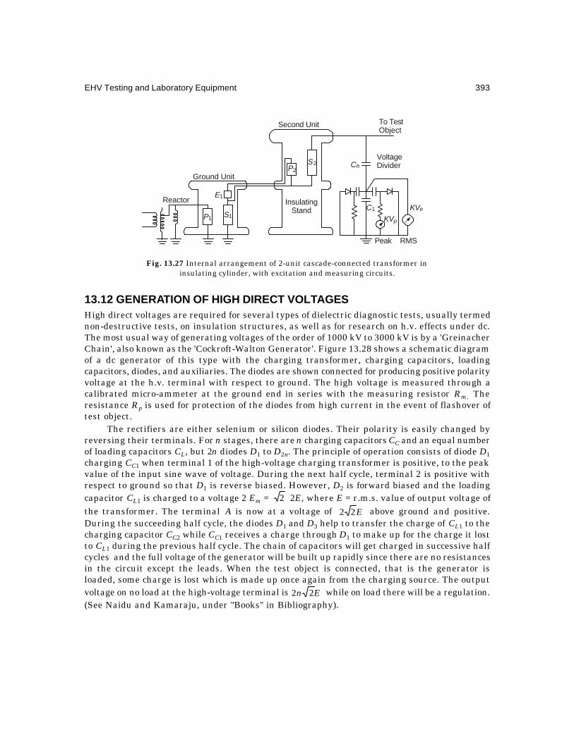
EHV Testing and Laboratory Equipment 393
Fig. 13.27 Internal arrangement of 2-unit cascade-connected transformer ininsulating cylinder, with excitation and measuring circuits.
13.12 GENERATION OF HIGH DIRECT VOLTAGESHigh direct voltages are required for several types of dielectric diagnostic tests, usually termednon-destructive tests, on insulation structures, as well as for research on h.v. effects under dc.The most usual way of generating voltages of the order of 1000 kV to 3000 kV is by a 'GreinacherChain', also known as the 'Cockroft-Walton Generator'. Figure 13.28 shows a schematic diagramof a dc generator of this type with the charging transformer, charging capacitors, loadingcapacitors, diodes, and auxiliaries. The diodes are shown connected for producing positive polarityvoltage at the h.v. terminal with respect to ground. The high voltage is measured through acalibrated micro-ammeter at the ground end in series with the measuring resistor Rm. Theresistance Rp is used for protection of the diodes from high current in the event of flashover oftest object.
The rectifiers are either selenium or silicon diodes. Their polarity is easily changed byreversing their terminals. For n stages, there are n charging capacitors CC and an equal numberof loading capacitors CL, but 2n diodes D1 to D2n. The principle of operation consists of diode D1charging CC1 when terminal 1 of the high-voltage charging transformer is positive, to the peakvalue of the input sine wave of voltage. During the next half cycle, terminal 2 is positive withrespect to ground so that D1 is reverse biased. However, D2 is forward biased and the loadingcapacitor CL1 is charged to a voltage 2 Em = 2 2E, where E = r.m.s. value of output voltage ofthe transformer. The terminal A is now at a voltage of E22 above ground and positive.During the succeeding half cycle, the diodes D1 and D3 help to transfer the charge of CL1 to thecharging capacitor CC2 while CC1 receives a charge through D1 to make up for the charge it lostto CL1 during the previous half cycle. The chain of capacitors will get charged in successive halfcycles and the full voltage of the generator will be built up rapidly since there are no resistancesin the circuit except the leads. When the test object is connected, that is the generator isloaded, some charge is lost which is made up once again from the charging source. The outputvoltage on no load at the high-voltage terminal is En 22 while on load there will be a regulation.(See Naidu and Kamaraju, under "Books" in Bibliography).
P1
E1
S1
P2Ground Unit
S2
InsulatingStand
Second Unit To TestObject
VoltageDivider
RMSPeak
Ch
C1 KVe
KVp
Reactor
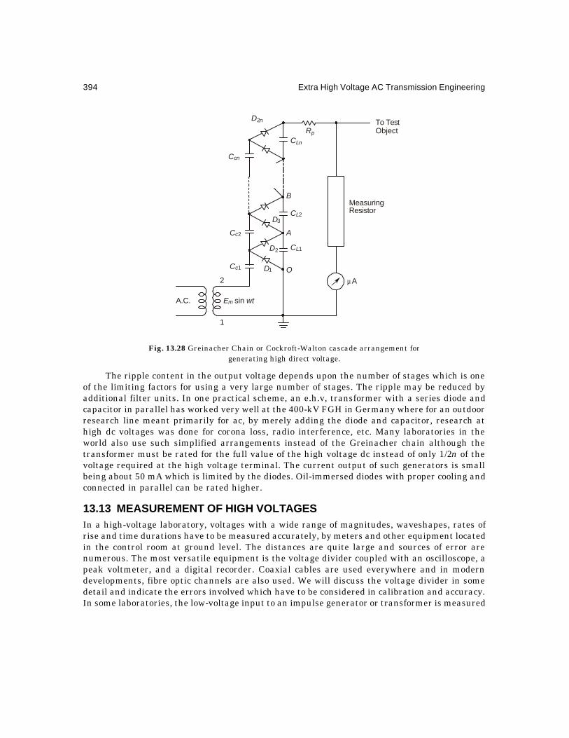
394 Extra High Voltage AC Transmission Engineering
Fig. 13.28 Greinacher Chain or Cockroft-Walton cascade arrangement forgenerating high direct voltage.
The ripple content in the output voltage depends upon the number of stages which is oneof the limiting factors for using a very large number of stages. The ripple may be reduced byadditional filter units. In one practical scheme, an e.h.v, transformer with a series diode andcapacitor in parallel has worked very well at the 400-kV FGH in Germany where for an outdoorresearch line meant primarily for ac, by merely adding the diode and capacitor, research athigh dc voltages was done for corona loss, radio interference, etc. Many laboratories in theworld also use such simplified arrangements instead of the Greinacher chain although thetransformer must be rated for the full value of the high voltage dc instead of only 1/2n of thevoltage required at the high voltage terminal. The current output of such generators is smallbeing about 50 mA which is limited by the diodes. Oil-immersed diodes with proper cooling andconnected in parallel can be rated higher.
13.13 MEASUREMENT OF HIGH VOLTAGESIn a high-voltage laboratory, voltages with a wide range of magnitudes, waveshapes, rates ofrise and time durations have to be measured accurately, by meters and other equipment locatedin the control room at ground level. The distances are quite large and sources of error arenumerous. The most versatile equipment is the voltage divider coupled with an oscilloscope, apeak voltmeter, and a digital recorder. Coaxial cables are used everywhere and in moderndevelopments, fibre optic channels are also used. We will discuss the voltage divider in somedetail and indicate the errors involved which have to be considered in calibration and accuracy.In some laboratories, the low-voltage input to an impulse generator or transformer is measured
To TestObject
D2n
RpCLn
CL2D3
D2
D1
CL1
Cc1
Cc2
Ccn
B
A
O
MeasuringResistor
1
2 µ A
E wtm sin A.C.

EHV Testing and Laboratory Equipment 395
instead of using a high-voltage divider, but this lacks accuracy. For routine testing of mass-produced equipment, such quick methods will be found quite adequate.
13.13.1 Voltage DividersThere are 3 types of dividers: (a) purely resistive divider; (b) a purely capacitive divider; and(c) resistance-capacitance divider. The former two are subject to serious limitations for e.h.v.work if precautions are not taken, which are overcome in the R-C divider.
Resistive Voltage Divider
Figure 13.29(a) shows a purely resistive divider consisting of a high-voltage arm Rh, a low-voltage arm R1 at the ground end, a cable with surge impedance Rc terminated at the oscilloscopeend by a resistance Rc equal to the surge impedance of the cable to prevent reflections from theopened end of the measuring cable. In high-voltage oscilloscopes, the vertical deflection circuitoffers almost infinite resistance and there is no resistance or capacitance at the input end as inconventional oscilloscopes. Standard co-axial cables available for measurement have Rc = 50ohms or 75 ohms.
The voltage ratio is
hv VVr /1= =cchh
c
cch
cc
RRRRRRRR
RRRRRRRRR
11
1
11
11
)/()/(
++=
+++
...(13.76)
Example 13.13. Calculate the divider ratio when a 20 kilohm high-voltage arm is connectedto a 100-ohm l.v. arm and the cable has Rc = 75 ohms.
Fig. 13.29 Resistive voltage divider. (a) Equivalent circuit. (b) Stray capacitances of divider.
Solution. The total l.v. arm resistance is 100 × 75/175 = 42.86 ohms.Therefore rv = 42.86/(20,000 + 42.86) = 1/467.6Also, 100 × 75/(20,000 × 175 + 100 × 75) = 1/467.6.At e.h.v. levels, the height of the high-voltage lead above the grounded floor of the laboratory
can be 20 metres so that inductances are present in the resistance. In addition, stray capacitancesare present which increase as the ground is neared. A realistic circuit of even a purely resistivedivider is depicted in Figure 13.29 (b). Screening of the resistor is therefore necessary to eliminatethese stray capacitances. An advantage of the resistive divider is the damping provided for
Vb
R1
Rh
Rc
RcV1
Cable
H.V. Load
ToScope
Rh
Ld
R1
Cd
( )b( )a
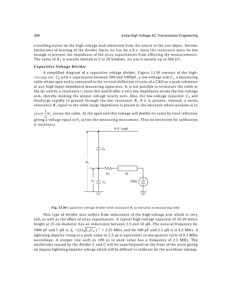
396 Extra High Voltage AC Transmission Engineering
travelling waves on the high-voltage lead connected from the source to the test object. Seriouslimitations of heating of the divider limits its use for e.h.v. since the resistance must be lowenough to prevent the impedance of the stray capacitances from affecting the measurements.The value of Rh is usually limited to 5 to 20 kilohms. Its use is mainly up to 500 kV.
Capacitive Voltage Divider
A simplified diagram of a capacitive voltage divider, Figure 13.30 consists of the high-voltage arm Ch with a capacitance between 300 and 1000pF, a low-voltage arm C1, a measuringcable whose open end is connected to the vertical deflection circuits of a CRO or a peak voltmeteror any high-input-impedance measuring apparatus. It is not possible to terminate the cable atthe far end by a resistance rc since this would offer a very low impedance across the low-voltagearm, thereby making the output voltage nearly zero. Also, the low-voltage capacitor C1 willdischarge rapidly to ground through the low resistance Rc if it is present. Instead, a seriesresistance Rc equal to the cable surge impedance is placed at the entrance whose purpose is to
place 121
V across the cable. At the open end this voltage will double its value by total reflection
giving a voltage equal to V1 across the measuring instrument. Thus no correction for calibrationis necessary.
Fig. 13.30 Capacitive voltage divider with resistance Rc at entrance to measuring cable
This type of divider also suffers from inductance of the high-voltage arm which is verytall, as well as the effect of stray capacitances. A typical high-voltage capacitor of 10-20 metreheight at 25 cm diameter has an inductance between 2.5 and 10 µH. The natural frequency for
1000 pF and 5 µH is 10 )2( −π= ddCLf = 2.25 MHz, and for 500 pF and 2.5 µH it is 4.5 MHz. A
lightning impulse rising to a peak value in 2.5 µs is equivalent to one-quarter cycle of 0.1 MHzwaveshape. A steeper rise such as 100 ns to peak value has a frequency of 2.5 MHz. Theoscillations caused by the divider L and C will be superimposed on the front of the wave givingan impure lightning-impulse voltage which will be difficult to calibrate for the wavefront timings.
H.V. Lead
Vh
Ch
Rc
C1 CROV1
Rc

EHV Testing and Laboratory Equipment 397
Another source of error with such tall slender equipment is that they might act as antennasto pick up r-f radiation from the numerous spark gaps in an impulse generator which formquite powerful spark transmitters. Another effect of these spark gaps in very large halls iscavity resonance. In most e.h.v. laboratories the radiation from these sparks is actually requiredin order to provide a deflection voltage without time delay to the horizontal deflection plates ofthe oscilloscope. The length of measuring cable connected to the vertical deflection plates thenacts as a delay line so that the vertical deflection voltage is impressed with some time delay toenable the full waveform to be viewed on the screen.
Example 13.14. Select the capacitance required in the l.v. arm of a capacitive divider toprovide a peak voltage of 500 volts at the oscilloscope when the high-voltage arm of the dividerhas Ch = 1000 pF and the voltage to be measured is 1200 kV, peak. Omit the cable surgeimpedance and Rc.
Solution. The required voltage ratio is
rv = ,2400
1
101200
500/1/1
/13
1
11 =×
=+
=hh CC
CVV
giving
C1/Ch = 2400 – 1 = 2399.Therefore C1 = 2399 × 10–9F = 2.399 hC2400F ≅µ .
Note that the low-voltage arm has higher capacitance which is almost equal to the high-voltage capacitance times the voltage ratio
C1 = (1/rv – 1) Ch.In order to reduce the inductance of the low voltage capacitor and its leads, the total
capacitance would be usually made up of several capacitors in parallel. In the above example, 6capacitors of 0.4 µF each might be soldered to heavy rings at both ends.
In section 13.5.1 and examples 13.3 and 13.4, it was shown how a switching-surge generatorrequires a higher loading capacitor CL in comparison to a lightning-impulse generator for thesame source capacitance Cs. The values were 12 nF instead of 2 nF for the two cases with Cs =83.3 nF. The capacitive voltage divider offers an advantage over a purely resistive divider byacting as an increased capacitive load and the same generator can deliver both a switchingsurge and a lightning impulse if a resistive divider is used for the latter. These can usually bearranged with a capacitor inside the insulating column surrounded by the high-voltage resistors.The low-voltage arm is provided with a switch which connects either a pure capacitance or aresistance. Proper switching of Rc must also be made for such cases.
Resistive-Capacitive Divider
Figure 13.31 shows the arrangement of resistances and capacitances in the high-voltagearm. The low-voltage arm could consist of a resistance and capacitance to match the high-voltage arm to provide the desired voltage division, but in most cases the very low value ofresistance required can be neglected and only a suitable value of low-voltage capacitor C1 issufficient.
The resistance serves a dual purpose. It helps to damp reflections in the high-voltage leadto the test object and critically damp the effect of series inductance in the divider column itself.Typical value of total resistance of a divider for 1200 kV is 100 ohms for a capacitance of 1000

398 Extra High Voltage AC Transmission Engineering
pF. This will critically damp any natural oscillation in the high-voltage arm having an inductance
of 2.5 µH )/2( ddd CLR = . The effect of Rd ddd LCR −− of the divider on the wavefront of a
lightning impulse has been fully analyzed in Section 13.6.3 and shown in Figure 13.12. Thepresence of Ld gives steeper rise of the front of the wave as compared to its absence.
Fig. 13.31 Resistance-capacitance voltage divider.
As mentioned earlier, the resistive or pure ohmic voltage divider cannot be normally usedfor measuring all types of voltage waveshapes because of the stray earth capacitance whoseeffect can be minimized if not eliminated by using screening electrodes or using a very lowvalue of resistance of the high-voltage arm. This will, in turn, have a limited thermal rating forthe very high voltages to be measured. In order to have a very low electrical time constant toreproduce the voltage faithfully, the product of resistance and effective stray capacitance mustbe low which again requires a low value of resistance. Furthermore, it cannot act as a load forgenerating composite waves (both lightning and switching) from the same generator.
For the purely capacitive divider, the stray capacitance to earth can be taken into accountin the overall response since it adds to the capacitance of the high-voltage arm. The purecapacitance, however, cannot damp oscillations caused by travelling waves or lead inductances.Therefore, a damped capacitive divider of the R-C type is found advantageous and has beenapplied for measuring voltage variations with as steep a rise to peak value as 100 ns = 0.1 µs,and for voltage magnitudes of several megavolts.
There are essentially two types of damped capacitive dividers: (1) the critically-dampeddivider; (2) the low-damped divider. Both these use series-connected sets of R-C elements. In
the critically-damped divider, the total resistance equals R = ed CL /2 , where Ld = inductance
H.V. Lead
R'
R'
R'
C'h
C'h
C'h
Ch
Rd
C1
Rc Rc
Cable
CRO


400 Extra High Voltage AC Transmission Engineering
In general the value of resistance required ranges from 400 to 1000 ohms for voltageshigher than 1 MV = 1000 kV. Ce is of the order of 50-150 pF and L is 5 to 10 µH.
(2) For a low-damped capacitive divider, the resistance is kept between 0.25 to 1.5 times
hh CL / , where now Lh = inductance of the entire loop of the high-voltage equipment andmeasuring system (which may be as much as 20 m × 20 m), and Ch = capacitance of the h.v. partof the divider only. In this case the h.v. lead has considerable inductance, and the resistanceused equals nearly its surge impedance. For a horizontal lead, the surge impedance is 120 ln(2H/r), where H = height of lead above a conducting plane and r = radius of lead. For a verticalrod, it is nearly 60 ln (2H/r) where H = height of the rod. Based upon these values, the timeconstant in the divider is kept below 100 ns for reproducing lightning impulses of 1.2/50 µs.This usually requires resistances in the range of 50 to 300 ohms for dividers meant for 1 MVand higher voltages.
Since the critically-damped divider requires a value of resistance higher than the surgeimpedance of the h.v. lead, it is connected at the h.v. terminal of the impulse generator. Thelow-damped divider, on the other hand, can be matched to the surge impedance of the lead andprovides a good compromise. When the impulse generator with the leads and divider is designedby the same manufacturer, optimum design can be achieved.
We now observe that the best compromise consists of the following scheme, Figure 13.33.In order to damp the oscillation occurring on the front of the impulse which is caused by thegenerator inductance, an internal series resistance in each stage amounting to a total of Rsi isnecessary. The wavetail-shaping resistor Rt is connected inside the generator in each stage. Apart of the wavefront-shaping resistor is connected as Rse at the head of the h.v. lead to thevoltage divider and test object located 15 to 20 m away. The voltage divider can be of low-damped or critically-damped type with an internal resistance Rd.
Fig. 13.33 Complete equivalent circuit of impulse generator with internal damping resistor Rsi,external series resistance Rse, wavetail-shaping-resistor Rt, damped R-C divider and test object.
13.13.2 The High-Speed OscilloscopeFor measuring lightning impulses and chopped waves, very high frequency response is necessaryin an oscilloscope. A 50 MHz oscilloscope is usually aimed at. For a full 1.2/50 µs wave, thehighest frequency component in a frequency spectrum goes to 1 MHz, and if the wave is choppedat 0.5 µs on the front the frequency required is 20 MHz. When used with voltage dividers, thefull-scale deflection of the oscilloscope ranges from 500 volts to 2000 volts so that impulseoscilloscopes must handle much higher voltages than conventional general purpose oscilloscopes.
E0
Cs
Rsi Rse
Rd
Cd
Ct ToScope
Rt
S G
+
LeadTo TestObject

EHV Testing and Laboratory Equipment 401
The horizontal deflection should be capable of being expanded to 2 µs full screen in order toview the wavefront properly.
Just as in all oscilloscopes used for viewing very fast phenomena, the vertical deflectionplates must get their voltage after a set time delay following the horizontal-axis deflectionvoltage. A delay line or circuit with very low attenuation is necessary. The delay provided by a
coaxial cable having dielectric of permittivity ε = 2.5 is Td = 98 1027.5103/5.2 −×=× sec =
5.27 ns per metre, since the velocity is proportional to the reciprocal of ε . Figure 13.34 showsthe T-arrangement required to match the cables to the two deflection plates with the incoming-cable surge impedance of Rc. When viewed from point P towards the oscilloscope, the impedance
must equal Rc so that cc RRRR =++ )(21
giving 3/cRR = . For 50-ohm cables, the resistance
to be connected in the T-junction is R = 32
16 ohms and for 75-ohm cables, the resistance to be
connected in the T-junction is R = 25 ohms.
Fig. 13.34 T-network for matching horizontal and vertical input cables tooscilloscope with cable from low-voltage arm of voltage divider.
When such matching T-networks are used, the vertical deflection requires a calibrationcorrection because the voltage drop in R is 33.3% of the voltage reaching the end of the lead atP. The deflection observed on the oscilloscope screen will be multiplied by 1.5 to obtain the truevoltage of the l.v. arm of the voltage divider.
This can be eliminated if the signal to the horizontal deflection plates is provided by othermeans. The scheme used is to pick up the radiated h-f energy from the large number of sparkgaps, which break down when the impulse generator is fired, by means of a rod antenna. Thisis connected to the horizontal deflection circuit of the oscilloscope through as short a length ofcoaxial cable as possible. The measuring cable from the l.v. arm of the voltage divider will thenact as a delay line or an artificial delay line can be provided for suitable time delay to thevertical deflection plates.
13.13.3 The Peak Voltmeter and the Sphere GapThe oscilloscope provides a picture of the waveshape of an impulse and offers a means ofchecking the timings and purity of the voltage as required by Standard Specification. Once this
Vert.Div
RcRc
R J
J
R
P
R
P
Rc Hor
R = Rc/3 23
Rc

402 Extra High Voltage AC Transmission Engineering
is verified and circuit constants adjusted suitably, it will only be necessary to have an indicationof the peak value of the voltage. For this purpose, a simpler instrument is used. Figure 13.35shows the schematic circuit diagram of a peak-measuring voltmeter. Here, the diode D willcharge the auxiliary capacitor Cm to the peak value of impulse which is obtained across the low-voltage arm of the voltage divider. This is indicated on a voltmeter PVM, or on a micro-ammeterconnected in series with the discharge resistor Rd. This resistance is necessary in order thatthe meter capacitance Cm can be ready for next impulse. A second diode can be used for theopposite polarity of the incoming signal.
Fig. 13.35 Circuit diagram of peak voltmeter.
Sphere gaps have been standard pieces of measuring equipment in a laboratory, but theyare now finding little or no use for e.h.v. needed for testing. The PVM and SG voltmeter cannotindicate the waveshape but only the peak values. In addition, a sphere gap can be adjusted tolimit the peak value of voltage across the test piece by suitably adjusting the gap length. Thesphere gap breakdown is very consistent and its accuracy is within 3%. Atmospheric correctionfactors are necessary where the breakdown voltage depends upon the air density factor
δ = ,1013
.273273
760.
273273 00 mmm b
ttp
tt
++=
++
...(13.80)
where t0 = 20°C, t = temperature in laboratory °C, pmm = barometric pressure in mm Hgand bm = barometric pressure in millibars. For lightning impulses, the breakdown voltage
varies directly with δ , while for switching surges it varies as 7.0δ . One may approximate thebarometric pressure to decrease by 7.5 mm or 10 millibars for every 100 metres increase inelevation. Temperature has very little effect on the pressure, but standard specifications mustbe consulted. According to Indian Standards, the temperature correction is
bm = 1013 (1 – 1.8 × 10⁻⁴t) ...(13.81)
13.13.4 The Digital RecorderA recent development in storing and displaying an impulse voltage waveform together with alltest details is the Digital Recorder, which uses the facility of fast sampling of µs-phenomenaand storing them. It is believed by those that have developed this instrument that it willeventually replace the high-speed oscilloscope, for impulse and other types of measurement inh.v. testing. [See No. 73, IEEE, in Bibliography].
Ch
ClCm Rd
D
e t( )
PVM
H.V. Lead
Vm
EHV Testing and Laboratory Equipment 403
A computer programmed to display all essential properties such as the peak value, timeto peak, front time, overshoot, time to 50% on tail, rate of rise in kV/µs, and any other desiredproperty facilitates analysis of the recorded waveform very easily. The waveform can be displayedon a computer graphic screen, stored on magnetic tape for future use, or a hard copy can beobtained for customer distribution or storage.
The waveform is sampled at a very high rate such as 10 ns/sample, and the use of 8-bitword length permits 28 = 256 discrete voltage levels to be recorded and stored. The only limitationfor high sampling rate is the band width of the digital recorders, which are however higherthan those of conventional oscilloscopes. Some high-frequency oscillation which is lost in anoscilloscope has been handled by the A/D converters in the Digital Recorder. Pre-triggeringphenomena, which occur before the waveform commences, can also be stored where necessary.
Because of the use of integrated circuits, which are influenced by the energy radiated bythe discharge of spark gaps in an impulse generator, these electronic circuits must be shieldedvery well, even though they may be installed in a Faraday cage enclosing the control desk andoperator. Ideally, the shield should be an entirely enclosed box made from thick sheet metalwith an extremely low resistivity. The currents induced in the metal will set up fields to counterthe external disturbing e.m. fields. Any obstruction to the flow of this current, such as holes orhigh-resistance welds and seams or doors with gaps, will reduce the effectiveness of the shieldedenclosure. Even the lead-in for cables will affect its performance. Research and development ofsuch Digital Recorders with display and storage is progressing rapidly and this is a very newtechnique.
13.13.5 Use of Fibre Optics in H.V. Measurements in Laboratories and Stations
Fibre optics and associated transmitter-receivers have now assumed very great importanceand wide use in high-frequency communication. Their insulating properties and freedom frome.m. interference make them excellent replacements for conventional coaxial cables for high-voltage measurements. Future measurements, control, and communication can be said tobelong to optical fibres. The sizes of e.h.v. switchyards and substations have become so largethat the length of control and communication cables are subject to interference due to ground-mat potential rise which could interfere even with proper relay operation. Furthermore, theuse of mini-computers and micro-processors are also subject to such potential rises andinterference. Optical technology can provide the electrical isolation required and freedom frominjected interfering noise. They also provide faster transmission or transfer of data thanconventional cables. Schemes are now under construction whereby carrier-type communicationand control can be carried out between generating and receiving stations by fibre optical links,since they can carry a very large number of channels. Microwave communication is impeded byhills and other obstructions which are eliminated with the use of fibre-optical links.
Optical fibres are also used in high-voltage laboratories for measurement of the extremelyhigh voltages. It has always been the practice to locate the low-voltage arm of the divider nearground in order to protect the measuring equipment and the operator from experiencing highvoltage. By the use of an optical-fibre link, the low-voltage arm can be placed at the highvoltage end of the divider thereby eliminating any stray capacitances caused by nearness to thelaboratory ground floor. An optical isolator is used to insulate the measuring equipment fromthe high voltage. This scheme uses a light-emitting diode (LED) which is energized from thevoltage developed across the low-voltage arm. The light intensity, modulated by the impulse or

404 Extra High Voltage AC Transmission Engineering
other waveform to be measured, can be made to fall on a photodiode or transistor which sendsthe signal through the optical fibre link to the measuring equipment. Optical isolators provideeffectively the insulating clearances.
13.13.6 Measurement of Partial DischargesLocalized electrical discharges inside high-voltage equipment are very important for their effecton insulation deterioration. They are the result of ionization in cavities or along the surfaces ofsolid dielectrics. Partial discharges give rise to corona-type pulses over a very wide frequencyrange, which are propagated from the source of partial discharge through circuit capacitancesin the windings of transformer and along the conductors. The measurement of these dischargesis recommended by IEC Publication No. 270, 1980 and in IS 2026: Power Transformers.
Fig. 13.36 Circuit for measurement of partial discharges
One example of the many schemes available is given in Figure 13.36. The measuringdevice M consists of an oscilloscope or a radio noise meter for displaying the q-V relationship asa Lissajous figure or the conducted noise in microvolts. In most transformers 1 pico coulombcorresponds to 1 µV on the noise meter, but this depends upon the capacitance of the windingfrom the source of p.d. to the high voltage terminal where the measuring system is located.
Voltage is applied to the object under test, E. The transformer must be free of partialdischarge up to the test voltage. A filter F is interposed between the transformer and testobject so that all energy in the partial discharge goes to the measuring system and none intothe source transformer which presents a low impedance to the h-f pulses. The p.d. pulses aretransmitted to the coupling capacitor and a damped tuned circuit consisting of the voltage-divider inductance and a resistor. The entire measuring system must also be free from partialdischarges. The coupling capacitor is filled with nitrogen at high pressure. The entire systemmust be enclosed in a Faraday cage and screened from external discharges. The design of aproperly shielded enclosure which prevents external e.m. disturbances from reaching the p.d.measuring equipment is a highly specialized topic and will not be discussed here. P.D.measurements are diagnostic tests and can give an indication of a fault that might developprogressively inside high voltage equipment such as transformers, cables and other equipmentusing very thick insulation.
Lf
Cf
50 HzA.C.
TestObject
C
L
R M

EHV Testing and Laboratory Equipment 405
13.14 GENERAL LAYOUT OF E.H.V. LABORATORIESWe end this chapter with some information on the design and layout of e.h.v. laboratories,chiefly of the indoor type. Outdoor laboratories for extremely high voltages are also used inorder to save the high cost of the building, but the equipment cost is higher. A combination ofindoor and outdoor laboratories also exists since some tests such as pollution and radiointerference require closed chambers. Outdoor equipment requires steel tanks and porcelaininsulator housing to guard against the elements. We shall give some examples of laboratorylayout. It is assumed that the highest voltages required in the testing equipment have beendecided by the designer based on the type of tests to be performed.
Clearances
The dimensions of laboratories will depend upon:
(a) the highest voltage for which the lab is designed,(b) the number of pieces of equipment required,
(c) the air gap clearances to be maintained, and
(d) the types of tests to be conducted and sizes of test objects.Over and above the requirement of a main hall, annexes have to be provided for research,
development and auxiliary equipment, as well as offices. The following recommended clearancescan be used as a guide for design.
(1) For Power Frequency TestsUp to 1000 kV a linearly increasing clearance of at least 4 metres will be necessary. The
50% flashover value of a rod-plane gap for power-frequency is given approximately by576.0
50 .652 dV = kV peak with d in metres. The following gap lengths are then necessary: 1000kV r.m.s. – 3.835 metres, 1500 kV – 7.754 metres, 2000 kV – 12.8 metres.
Example 13.15. An airgap clearance is to be designed for a withstand voltage of 1500 kV,r.m.s. The withstand voltage is 80% of 50% flashover voltage. For a rod-plane gap, calculate theminimum clearance required.
Solution. 50% flashover voltage = 8.0/21500 = 2651.65 kV, peak.Therefore, 2651.65 = 652.d0.576 giving d = 11.42 metres.(2) Lightning-Impulse ClearancesFor voltage up to the highest value used for lightning-impulse tests (6 to 7 MV) the required
clearance rises linearly with voltage, as has been discussed in Chapter 11. A clearance of 2metres for each 1000 kV is necessary. The impulse flashover formula is V50 = 500d for a rod-plane gap (V50 in kV and d in metres). The withstand voltage can be assumed to be 80% of V50,so that a 2-metre gap will withstand 800 kV, crest. For other types of gap, the same gap lengthcan withstand higher values of voltage.
(3) D.C.A clearance of 4 metres for every 1000 kV is recommended.(4) Switching SurgesA given electrode geometry exhibits the weakest electrical strength for positive-polarity
switching surge, as described in chapter 11. The recommended clearance is d = 4(MV)2, whichgives 4 metres for 1000 kV crest and 16 metres for 2000 kV, crest.

406 Extra High Voltage AC Transmission Engineering
The rod-plane CFO is V50 = 500.d0.6 kV crest according to Paris's formula. This yields d =3.2 m for 1000 kV and 10.1 metres for 2000 kV, crest. With the withstand voltage being 80% ofCFO, the clearances required are 4.6 m for 1000 kV withstand and 14.6 m for 2000 kV withstand.
General LayoutThe clearances given above will help to dimension the layout of equipment. In order to
reduce the size required for a hall, one might observe that there is no need for using all thesources of high voltage simultaneously. For example, very rarely if ever is a switching impulsetest carried out simultaneously with power-frequency test. This enables the transformer to bemoved out of its permanent location during tests, if it is mounted on wheels. Similarly, for theimpulse generator. When this philosophy is adopted, it is sufficient to construct the floor ofsteel and pave it with smooth cement. An arrangement for supplying a cushion of pressurizedair under the base of the heavy equipment will facilitate easy movement. The approximateweight of a 2000-kV power frequency transformer for indoor use of the insulating-cylinder typeis 100 Tonnes. An impulse generator for 6 MV and 30 kJ weighs 25 Tones approximately.
Large halls have a metallic screen in their walls to act as shield in order to prevent e.m.radiation from sources external to the building, such as ignition spark radiation etc., enteringthe hall thereby disturbing sensitive measurements such as partial discharges and radiointerference (RIV) in the µV range at 0.5 to 1.5 MHz. However, with the very large number ofspark gaps discharging the impulse generator, this metallic shield in the walls will reflect theenergy back into the hall and disturb not only RIV measurements but also the steep-risingfront of the lightning impulse itself. This effect is known as Cavity Resonance. A semiconductingcoating on the inside of all walls of the huge hall will prevent the re-radiation. Many laboratorieshave used chicken-wire mesh on the inside. An outdoor laboratory is free from cavity resonancebut it will be subject to e.m. interference from sources outside laboratory area such as passingvehicles (ignition radiation), welding equipment nearby, motors, etc. In every case, therefore,a compromise has to be effected such as constructing specially-shielded rooms for sensitivemeasurements and lead the high-voltage connection through a wall bushing from an outdoorgenerator. Such bushings are very heavy and long, requiring proper support.
Grounding grids in e.h.v. laboratories and earthing wells need very special care. It isconsidered beyond the scope of this book to deal with this problem.
Example 13.16. Design a possible layout of a laboratory to be equipped with the followinghigh-voltage equipment. Other specifications are also supplied.
(1) Lightning and Switching Impulse Generator4000 kV output voltage. Charging voltage per stage 200 kV, stage capacitance 1.5 µF,
energy 30 kJ, number of stages 20. Generator height 15 metres, electrode height 2m. Requiredclearances: Lightning 8m, switching 26 m. Generator base 3 m on side.
(2) Power Frequency Transformer3-unit cascade, 1500 kV, 1A. Insulated cylinder type. Approximate height to the top of the
high-voltage electrode –15 m. Required clearance is 8 m all round. Provide one more groundunit for higher current output connected in parallel with the first or base unit of 3-unit cascade.Clearance = 3m. Bases: 1500 kV – 5m on side. 500 kV – 3.5 m on side.
(3) D.C. Generator2000 kV, 10 mA. Height 10 m, base 2 m on side.(4) Voltage DividerSame height as impulse generator. Distance from generator = 20 m.

EHV Testing and Laboratory Equipment 407
(5) Space for Test Object10 m along the length of hall.(6) Control RoomAs annexe to the main hall. 15 m long, 6 m wide.Solution.Figure 13.37 shows a possible plan and elevation of the laboratory showing dimensions of
equipment and required clearances. No attempt has been made to move equipment from theirpermanent locations. The main points to note are the following: clearance from IG to walls – 26m for switching surge. Distance between IG and Voltage divider – 20 m. IG to DC set – 18 m.
Clearance from IG to test object – 18 m.Distance from 50 Hz transformer cascade to wall – 8 m; to voltage divider – 5 m.Compensating reactor are placed against walls.
Fig. 13.37 Plan and elevation of general layout of a e.h.v. laboratory for 4000 kV impulse,1500 kV power frequency and 2000 kV dc voltage.
Reactors
Control
15
6
10
18
26
26
26
57 m
43
67 m
67 m
50 HzTrans
TestArea
V.D.
I.G.
1217 17 15
50 HzV.DI.G
18

408 Extra High Voltage AC Transmission Engineering
Review Questions and Problems
1. What are the standard waveshapes used for the following types of surges? (a) Lightningvoltage, (b) Lightning Current, (c) Switching impulse for testing line material,(d) Switching impulse for transformer tests. Give neat sketches and indicate allmagnitudes and timings.
2. A double-exponential voltage rises to peak value in tm = 0.1 µs and falls to 50% valueon tail at tt = 0.3 µs. Determine its equation )()( tt eeEte β−α− −= by calculating E/VP,α and β . What type of voltage is this?
3. An impulse generator with source capacitance Cs = 125 nF and load capacitance 5 nFis required to generate a double-exponential voltage of 1.2 µs/50 µs. Calculateapproximately the values of front and tail resistances Rf and Rt.
4. What are the three places where inductance is present in an impulse generator?Discuss their effect on measured waveforms of voltage by a voltage divider.
5. What is a critically-damped divider and an under-damped divider? Where are theyused?
6. In problem 3, there are 12 capacitors with each stage having 125 nF capacitance andthe charging voltage per stage is 200 kV. Calculate its energy when (a) all stages areconnected in series, (b) the stages are re-connected with 2 capacitors in parallel in 6stages, (c) all 12 capacitors are connected in parallel into 1 stage.
7. An impulse current generator has 6 impulse capacitors each of 0.2 µF in parallel. Thedesired waveshape is tm = 8 µs and tt = 20 µs. Calculate (a) the approximate values ofresistance and inductance allowable in the circuit to generate double-exponentialcurrent waveform and (b) the charging voltage to obtain 15 kA through an arresterwhose residual voltage stays constant at 20 kV, peak.
8. Draw a neat diagram of an insulating cylinder type of cascade-connected transformerwith 3 stages showing power input, the windings with internal compensating reactorsand measuring circuits.
9. A pure capacitive divider has high-voltage arm of 495 pF rated for 2.4 MV. The dividerratio is 990/1. Calculate the value of capacitance of the low-voltage arm and its voltagerating.
10. Draw the circuit diagram of a peak voltmeter and explain the principle of operation.See D. Kind, under "Books" in Bibliography.
14.1 INTRODUCTIONThis chapter will be devoted to a discussion of the application of all the material of previouschapters to evolve methods of design of e.h.v. lines. Two important governing factors stressedhere are (1) steady-state operating limits, and (2) insulation design based upon transientovervoltages. Other problems usually associated with transmission lines are (a) transient anddynamic stability, and (b) short-circuit currents and voltages. These depend on the characteristicsof the connected generating stations and system inter-connection and cannot be discussedhere. But such a study has to be conducted after the line is designed and some factors mighthave to be modified.
High-voltage insulation problems can be generalized in sequential steps when the systemtransient studies are conducted and the air-gap insulation characteristics are understood tooffer a proper level of safe operation which is determined on a probability basis of allowing acertain level of line outages. But the steady-state compensation requirements depend upon thepower transmitted and line length. The different types of reactive-power compensation discussedin Chapter 12 can be divided into the following categories:
(1) Lines for which compensating equipment is provided at only the receiving-end of theline across the load. Such schemes use synchronouse condensers, switched capacitors,static Var systems and regulating transformers with on-load tap-changing facility.These lines are short.
(2) Those for which static shunt-reactor compensation is required at no load conditionsfor voltage control at the two ends. These are permanently connected and switchedcapacitors across the load take care of compensation required for load variation atthe receiving end. These lines can be termed medium length in so far as e.h.v.transmission is concerned.
(3) Conditions for which the load requirement necessitates series-capacitor compensationalong the line in addition to shunt-reactor compensation at the ends for voltage controlon no load. Switched capacitors will take care of load conditions for voltage control.These lines can be considered as long.
14Design of EHV Lines Based upon Steady State
Limits and Transient Overvoltages

410 Extra High Voltage AC Transmission Engineering
(4) Lines which necessitate an intermediate switching station where shunt reactors areprovided in addition to series capacitors in the two line sections along with shunt-compensating reactors for no-load conditions across the source and load. These areextra-long lines.
The theory and analysis of these types have been covered in Chapter 12. Air gap insulationcharacteristics have been dealt with in Chaper 11. We will discuss design procedures throughexamples of several types of lines based upon the principles set forth in all the earlier chapters.The governing criteria for line design are postulated below and discussed further.
14.2 DESIGN FACTORS UNDER STEADY STATEAll designs can be considered as synthesis of analytical procedures that are available and anenumeration of the limits and constraints under which line designs have to be carried out. Thesteady-state considerations are the following:
(a) Maximum allowable bus voltages and across equipment for a given voltage level.These are specified by Standards and given in Chapters 2 and 11.
(b) Current density in conductors which determine the cross sectional area, the resultingtemperature rise, etc. These were discussed in Chapter 3.
(c) Bundling, corona-inception gradient, and energy for these factors are important forfixing the conductor diameter and number of conductors in the bundle and have beendiscussed in Chapters 4 and 5.
(d) Electrostatic field under the line at 50 Hz covered in Chapter 7.
(e) Audible noise and radio interference discussed in Chapters 5 and 6.
( f ) Compensation requirements for voltage control as described in Chapter 12.
A summary of equations and constraints can be given here.(a) The limits for maximum operating voltages are as follows:
Nominal System kV 220 345 400 500 735–765 1000 1150
Maximuim Equipment kV 245 362 420 525 765 1050 1200
The power-handling capacity of a single circuit can be assumed for commencing the designto be P = 0.5 V 2/Lx, MW/circuit with V in kV, line-line, L = line length in km, and x = totalseries reactance per km per phase. The % power loss is P = 50 r/x, where r = line resistanceper km per phase. Based on the total power to be transmitted, the number of circuits can bedecided for a chosen voltage level. Several voltage levels should be selected and alternativedesigns worked out, since design requirements vary from location to location. It has beendiscussed earlier that one 1200–kV circuit can carry as much power as 3–750 kV lines and 12–400 lines for the same distance of transmission.
(b) Current density normally encountered lies between 0.75 A/mm2 to 1 A/mm2. At thelower values for carrying the same current (determined by power per circuit andchosen voltage level) conductors tend to be larger than at the higher value of currentdensity which reflect on the surface voltage gradient and corona effects.
(c) Charge of bundled conductors governs the electrostatic field in line vicinity, the surfacevoltage gradient on conductors and the resulting RI, AN, and corona loss. The chargeper unit length on the 3-phase conductors is ],][[2][ 0 VMeq π= where the voltage

Design of EHV Lines Based upon Steady State Limits and Transient Overvoltages 411
matrix is tVV ]1201,1201,01[][ °∠°−∠°∠= in the steady state with V = r.m.s. value ofline-to-neutral voltage in volts. The matrix ,][][ 1−= PM where [ P ] is the Maxwell'spotential-coefficient matrix with the elements .)/ln(),/2ln( jiAIPrHP ijijijeqiii ≠==Here Hi = height of conductor i above ground, Iij = distance between conductor i andthe image of conductor j, Aij = aerial distance between conductors i and j, and req =geometric mean radius or equivalent radius of bundle = =NRrNR N ,)/.( /1 numberof sub-conductors, r = sub-conductor radius, R = bundle radius, and i, j = 1, 2, 3.
The resulting inductance matrix is [L] = 0.2 [P] mH/km (or µ H/m), and the capacitance
matrix is ],[2][ 0 MeC π= Farad/m (the factor ,F/m1055.5518/102 1290
−− ×==πewhere .F/M)842.80 µµ=e
For the 3 phases,
°∠+°−∠+°∠=π°∠+°−∠+°∠=π
°∠+°−∠+°∠=π
]1201200[2/
]1201200[2/
]1201200[2/
33323103
23222102
13121101
MMMVeqMMMVeq
MMMVeq
...(14.1)
(d) Electrostatic FieldThe horizontal and vertical components of field are determined at a point A(x, y)where x and y are its coordinates with reference to a chosen origin. A convenientlocation is at ground under the centre phase. Then:
(i) Vertical component due to phase i will be
)(iEv = ])/()(/)).[(2/( 2'20 iiiii DyHDyHeq ++−π ...(14.2)
(ii) Horizontal component is
)(iE h = ])/(1/1)[)(2/( 2'20 iiii DDxxeq −−π ...(14.3)
where ix = horizontal coordinate of phase i,
2iD = 22 )()( ii Hyxx −+−
and 2' )( iD = 22 )()( ii Hyxx ++− ...(14.4)
(iii) The total field is
2iE = 22 )]([)]([ iEiE hv ∑+∑ ...(14.5)
(e) Conductor Surface Voltage GradientThe quantity qi calculated earlier is the charge of the entire bundle. The maximumsurface voltage gradient on any sub-conductor will be
Emax = ]/)1(1)[/1).(/1).(2/( 0 RrNrNeqi −+π ...(14.6)
For most practical calculation, the Mangoldt Formula (Markt-Mengele Formula) canbe used for horizontal configuration of the three phases (Chapter 4).

412 Extra High Voltage AC Transmission Engineering
( f ) Corona-Inception GradientFor a cylindrical conductor above a ground plane, Peek's formula for corona-inceptiongradient is
E0 = r.m.s.kV/m,)/0301.01(..2140 δ+δ rm ...(14.7)
where m = conductor surface roughness factor < 1
δ = air-density factor ttb
++=
273273
10130
r = conductor radius in metre,b = barometric pressure in millibars,t = temperature °C
t0 = reference temperature, 20°C presently used, but will become27°C when adopted in future.
The barometric pressure varies with elevation and temperature dropping by 10millibars for every 100 metre increase in elevation. The temperature correction isinsignificant. The value of m = 0.7 to 0.8 in fair weather and 0.55 to 0.65 in rain.
( g ) Radio Noise Level (Chapter 6)
For up to 4 conductors in bundle, the C.I.G.R.E. formula isRI(k) = 0.035 Em(k) + 1200 r – 33 log (D(k)/20)–30 dB ...(14.8)
where Em(k) = maximum surface voltage gradient on sub-conductor in kV/m, r.m.s.,D(k) = aerial distance from phase k to the point where RI is evaluated and k = 1, 2, 3.
Rules for adding RI due to all phases are given in Chapter 6. For 1 MHz level, deduct 6 dBfrom equation (14.8).
(h) Audible Noise (Chapter 5)For N < 3, AN(k) = 120 log Em(k) + 55 log (2r) – 11.4 log D(k)
– 245.4, dB (A) ...(14.9)For N ≥ 3, AN(k) = 120 log Em(k) + 55 log (2r) – 11.4 log D(k)
+ 26.4 log N – 258.4, dB (A) ...(14.10)The total AN level of the 3 phases is
AN = 10 log ∑=
3
1
)(1.0 dB(A),10k
kAN...(14.11)
(i) Corona Loss. (Ryan and Henline Formula, Chapter 5).WL = 4fC V(V – V0) MW/km, 3-phase. ...(14.12)
(j) Voltage Control at Power Frequency (Chapter 12).
(i) Line only:
s
s
IE
=
r
r
I
E
DC
BA
,
,...(14.13)
A = D = cosh pL = cosh ZY

Design of EHV Lines Based upon Steady State Limits and Transient Overvoltages 413
=−==
==
.1
sinh.//sinh
sinh./sinh
0
0
BCADZYZYZpLC
ZYYZpLZB
...(14.14)
Z = (r + jwl) L, Y = jwcL. ...(14.15)r,l,c = distributed resistance, inductance and capacitance per km
L = line length in kmw = fπ2
(ii) Shunt Reactor Compensation. Reactor admittance = BL.
−
−
=
BBjBAOB
jBDCBA
DCBA
LL
lineTT
TT
,2
,
,
,
,
,...(14.16)
(iii) Series Capacitor Located at Centre and Shunt Reactors at ends.
−
−
=
BBjBAOB
jBDCBA
DCBA
LL
lineTT
TT
,2
,
,
,
,
,
++−
+− pLpLjBpL
Z
OpLBX
LLc cosh1),cosh1(sinh
2,cosh1
21
0
–
+pLZpL
ZpLpLZ
jX c
sinh/)1–(cosh
/)1(cos,sinh
2 0
0
0...(14.17)
Limits. The following limiting values will govern the design of line and the width of linecorridor required.
( a) Electrostatic Field. Ground-level maximum value is 15 kV/m, r.m.s.
( b ) Radio Interference. 40 dB above 1 µ V/m at 1 MHz in fair weather at the edge ofR-O-W.
( c ) Audible Noise. 52.5 dB (A) at edge of R-O-W.(d ) Corona–Inception Gradient. Margin above maximum voltage gradient is at least
10% on centre phase or the phase with maximum voltage gradient.( e ) Corona Losses. With corona-inception gradient being above maximum voltage
gradient at the operating voltage, no corona loss is anticipated in fair weather.But check in rain.
( f ) Line Compensation. This must be designed to hold the bus voltage within limitsgiven by Standard Specification.
14.3 DESIGN EXAMPLES: STEADY-STATE LIMITSThe above criteria and equations for all quantities under steady state operating conditions ofline will be applied for design of the following lines.

414 Extra High Voltage AC Transmission Engineering
(1) 400 kV 200 km line to transmit 1000 MW using synchronous condenser at load end.
(2) 400 kV 400 km line to transmit 1000 MW using shunt-reactor compensation at bothends for no load condition and switched capacitors for load condition for voltage controlat buses.
(3) 400 kV 800 km line to transmit 1000 MW using 50% series capacitor compensation atline centre, shunt reactors at both ends for voltage control at no load, and switchedcapacitors across load.
(4) 750 kV 500 km line for transmitting 2000 MW with only shunt-reactors at ends forvoltage control at no load and switched capacitors under load.
14.4 DESIGN EXAMPLE—I (400 kV, 200 km, 1000 MW)(1) Number of CircuitsWith equal voltage magnitudes at both ends to commence the design and 30° phase
difference between them, the power-handling capacity per circuit is with x = 0.327 ohm/km,P = 0.5 × 4002/0.327 × 200 = 1223 MW, 3-phase.
Therefore, one circuit will be sufficient.
(2) Line Clearance and Phase SpacingNESC recommends a minimum clearance of 29 feet = 8.84 metres based on 17' for first
33 kV and 1' extra for each 33 kV above this or part thereof. The sag is expected to be 12 m.Therefore, average height for calculation of potential coefficients is H = 9 + 12/3 = 13 m
in horizontal configuration. The phase spacing required from switching surge considerations isexpected to be 12 m. At maximum swing of insulators it should be 7.5 m. Allow 4.3 metreheight for insulator string and 30° swing. This aspect will be taken up in Section 14.8 underDesign Based upon Transient Overvoltages.
(3) Conductor Size and Number in BundleThe twin conductor has become the accepted standard for 400 kV, although one line in
Germany (Rheinau) uses 4 conductors in bundle in 4-circuit configuration. We first try thedouble Morkulla or Moose with r = 0.0159 metre radius at bundle spacing of B = 0.4572 metre.This will be checked for (a) corona-inception gradient and (b) margin between this and themaximum surface voltage gradient. Using Mangoldt formula,
For the Centre Phase
Emc = ]4/2ln../[]/)1(1[ 22 SHrHSrNRrNV eq +−+ ...(14.18)
Here, V = kV3/420 at the maximum operating voltage,
N = 2, R = 0.2286, r = 0.0159, H = 13, S = 12
req = m.08526.0=rB
Therefore, Emc = 85.40159.0207.1
3
420××
= 1681.5 kV/m = 16.815 kV/cm

Design of EHV Lines Based upon Steady State Limits and Transient Overvoltages 415
For the Outer Phases
Emo = [ )/2/[ln(]/)1(1. eqrHRrNrN
V−+
++− 22222 /))(4(ln5.0 SSHSH ...(14.19)
= 1601.5 kV/m = 16.015 kV/cm.
Corona-Inception Gradient ( ).1=δat Take m = 0.75
Eor = kV/m198875.0)0159.0/0301.01(2140 =×+
Margin. For the centre phase, (1988 – 1681.5)/19.88 = 15.42%. For the outer phases, (1988
–1601.5)/19.88 = 19.44%. These are considered satisfactory.
(4) RI LevelAt 15 m from the outer phase at ground.
Emc = 16.82 kV/cm, Emo = 16.02 kV/cm.
D(1) = ,m302713)2(,m85.191513 2222 =+==+ D
D(3) = )m20)1(:(.m1.413913 22 ≈=+ DNoteTherefore,
RI(1) = 0.035 × 1602 + 1200 × 0.0159 – 30 = 45.15 dB
RI(2) = 0.035 × 1682 + 19.08 – 30 – 33 log (30/20) = 42.14 dB
RI(3) = 0.035 × 1602 + 19.08 – 30 – 33 log (41.1/20) = 34.83 dB.
Therefore, RI level of line = 45.15 dB at 0.5 MHz and 39.15 dB at 1 MHz. This is consideredsatisfactory since the limit is 40 dB at the edge of R-O-W. The line corridor can therefore bemade equal to 2(S + 15) = 54 metres.
(5) Audible NoiseAt 15 m from outer phase at ground.
AN(1) = 120 log 1602 + 55 log 0.0318 –11.4 log 19.85 – 245.4= 42 dB (A)
AN(2) = 120 log 1682 – 82.37 – 245.4 – 11.4 log 30 = 42.5AN(3) = 120 log 1602 – 82.37 – 245.4 – 11.4 log 41.1 = 38.4
Therefore,AN = 10 log (104.2 + 104.25 +103.84) = 46.08 dB (A)
This is less than the limiting value of 52.5 dB (A) and the line corridor governed by RI canbe considered as adequate.
(6) Electrostatic FieldThe Maxwell Potential coefficient matrix has the elements
Pii = ln (26/0.08526) = 5.716, Poc = ln and87.0)12/1226( 22 =+
416 Extra High Voltage AC Transmission Engineering
P00 = .39.0)24/2426ln( 22 =+
Therefore, [P] =
716.587.039.0
87.0716.587.0
39.087.0716.5
,
giving [M] =
−−−−−−
=−
1728.0026.0008.0
026.01772.0026.0
008.0026.01728.0
][ 1P
Then, at V = ,kV3/420
π
π
π
03
02
01
2/
2/
2/
eq
eq
eq
= 3
420
1201728.0120026.00008.0
120026.01201772.00026.0
120008.0120026.001728.0
°∠+°−∠−°∠−°∠−°−∠+°∠−
°∠−°−∠−°∠
At a distance d along ground from the line centre, the vertical component of e.s. fieldcomes out to be
Eu =
−++
+−
++ 222222 )(
116.26416.2
)(
94.4
3
420
SdHdHSdH
−++
+−
+++
222222 )(
472.4576.4
)(
398.0
SdHdHSdHj
The maximum value occurs at d = 1.05 H = 13.65 metres from line centre and is 4.7 kV/m. This is below the limit of 15 kV/m for safe let-go currents.
(7) Corona LossSince an ample margin is given between the corona-inception gradient and the maximum
surface voltage gradient on conductors, no corona loss is anticipated at the design stage in fairweather.
(8) Line Compensation RequirementsFrom the [P] and [M] matrices, the average values of positive-sequence inductance and
capacitances are calculated as follows:Ls = 0.2 Pii = 1.144 mH/km,
Lm = 0.2 (2 × 0.87 + 0.39)/3 =0.142 mH/kmTherefore,
L+ = )H/m(.mH/km1142.0144.1 µ≅−=− ms LL
X+ = ohm/km.314.02 =π +fL
Cs = 3/)1728.01772.01728.0(18
102
9
0 ++=π−
iiMe = 9.68 nF/km (pF/m).
Design of EHV Lines Based upon Steady State Limits and Transient Overvoltages 417
Cm = oeπ2 ( – 0.026 – 0.008 –0.026)/3 = – 1.11 nF/km
Therefore,
C+ = Cs –Cm = 9.68 + 1.11 = 10.79 nF/km
y = wC+ = 3.39 × 10⁻⁶ mho/km
r = 0.023 ohm/km
For L = 200 kmZ = 4.6 + j62.8 = 62.97 ∠ 85°.8 ohm. Y = j0.68 × 10–3 mho
Therefore,Z0 = ,1.23.304)/( 2/1 °−∠=YZ
ZY = 0.207 ∠ 87°.9 = 0.0076 + j0.2069
cosh ZY = 0.9787 + j0.00156 = 0.9788 ∠ 0.09°
sinh ZY = 0.0074 + j0.2055 = 0.2056 ∠ 87°.94.For the line, A = D = 0.9788 ∠ 0.09°, B =62.56 ∠ 85°.84,
C = 0.6756 ∠ 90° × 10–3.As a first assumption, let the receiving-end voltage Er = 420 kV. Then , centre of the
receiving–end circle diagram is at
xc = – | MW5.204)cos(|/2 −=θ−θ abr BAE
yc = – | MVAR2752)sin(|/2 −=θ−θ abr BAE
Radius R = | ./,2820.|/ rssr EEmwhereMVAmBEE ==The receiving-end circle diagram is drawn for several values of m ranging from 0.8 to 1.0.
The load line is drawn at 1000 MW at unity power factor. At no load, the reactive powerrequired is found as Qor which is inductive. At full load, the capacitive reactive power is alsodetermined as QLr. The value of m that gives Qor/QLr = 0.7 will give the required value of Eswhen a synchronous condenser is utilized for compensation. The two equations are from Figure14.1,
2222 2820|)|( mxyQ ccor =++ ...(14.20)
and 2222 2820)|(||)|1000( mQyx Lrcc =−++A value of m = 1.0162 gives the desired ratio Qor/QLr = 0.7 with inductive compensation of
Qor = 106.4 MVAR at no load and capacitive compensation of 151.8 MVAR at full load of 1000MW at unity power factor. The sending-end voltage will then be Es = 1.0162 × 420 = 426.8 kV.This is 6.8 kV higher than allowed by Standard Specification. Therefore, the receiving-endvoltage should be taken to be less than 420 kV and the compensation requirement re-worked.
A second trial could start at ER = 400 kV.xc = –185.5 MW, yc = – 2496.4 MVAR, R = 2557.5m MVA.
The equations for Qor and QLr are found to be
Qor = and,4.24965.185)5.2557( 22 −−m
QLr = 22 5.1185)5.2557(4.2496 −− m

418 Extra High Voltage AC Transmission Engineering
For m = 1.023 or Es = 409.2 kV, there result Qor = 113 MVAR inductive and QLr = 164MVAR capacitive giving a ratio Qor/QLr = 0.69. This is satisfactory. The synchronous condenserrating will be approximately 165 MVAR leading for over excitation and 115 MVAR lagging forunder-excited operation. The bus voltages are 400 kV at the receiving end and 409.2 kV at thesource end. These are within the limits specified by Standards.
Fig. 14.1 Compensation calculation for Design Example No.1.
The power angle at full-load operation is
δ = °=−=+
−−θ 84.216384.85
1000arctan
c
Lrcb x
Qy
The analytical equations for (Es, Is) in term of (Er, Ir) are given below:
s
s
IE
=
r
r
IE
DCBA
,
,...(14.21)
Now, Er = 400 kV ,0°∠ line-line.The total load at the receiving end is
Wr = Pr + jQr = 1000 = j 164 MVA, 3-phase.Therefore,
Ir = 4003/)1641000()*/( ×+= jEW rr
= 1.443 + j 0.237 kiloamperes per phase
= 1.462 ∠ 9.33° kA.Therefore,
Es = 33.9462.184.8556.623
40009.09788.0 °∠×°∠+×°∠
= 236.73 ∠ 22.73°, kV line-to-ground = 410 kV, 1–1
Qor
QLr
1000 MW
yc
R = 2820 m
CPL(–204.5, – 2752)

Design of EHV Lines Based upon Steady State Limits and Transient Overvoltages 419
Therefore, δ = 22.73 as compared to 21.84 from the circle diagram,
Is = kA,33.9462.109.09788.03
400106756.0 3 °∠×°∠+×× −j
= 1.4984 ∠ 28°.33 = 1.319 + j 0.711 kA.
The sending-end power is
Ws = 33.2873.224984.141033 * °−°∠××=ssIE
= 1059 – j 103.84 MVA
Therefore the line loss is P = 1059 – 1000 = 59 MW, 3-phase
The % line loss is P = 59 × 100/1059 = 5.57% and the efficiency of transmission inη = 1000 ×100/1059 = 94.43%
14.5 DESIGN EXAMPLE-II: 400 kV, 400 km, 1000 MW WITH SHUNTCOMPENSATION
Using P = 0.5 × 4002/400 × 0.327 = 640 MW, we find that 2 circuits may be necessary to handle1000 MW. Design will be based on 500 MW/Circuit.
The high-voltage effects will be the same as the example in Sec. 14.4 for the 200-km line.Only the compensation requirements will be different.
No-Load CompensationFor control of voltage at no load, shunt reactors of 50 MVAR each at both ends will be
used. This is a recommended practice in India. But the bus voltages should be checked forother reactive powers. As shown in chapter 12, the total generalized constants are
AT = ABjBBCCBBBjBAD LLTTLT 2,, 2 −−==−= ...(14.22)
where A, B, C, D pertain only to the line.
For 400 km, Z = 9.2 + j 124 ohm, Y = j 1.36 × 10⁻³ mho
Z0 = .88411.0,1.23.302 °∠=°−∠ ZY
Therefore,
cosh ZY = .1.884.0sinh,36.0917.0 °∠=°∠ ZY
For the line, A = D = 0.917 ∠ 0.36°, B = 120.77 ∠ 86° andC = 1.4 × 10⁻³ ∠ 87.8°
At 50 MVAR 3-phase and 400 kV, line-to-line, each shunt reactor has an admittance of BL= 0.312 × 10⁻³ mho. This gives AT = DT = 0.955.
Selecting a sending-end voltage Es = 400 kV, the load-end voltage will be Er = Es/AT =418.85 kV, which is below the maximum allowable 420 kV.
Now, BT = °∠×=−−=°∠= − 8610817.02and8677.120 32 jABjBBCCB LLT
Therefore, the percentage compensation afforded by the shunt reactors is (1.4 – 0.817)100/1.4 = 41.6%, which is considered satisfactory. Normal values lie between 40% and 60%.
420 Extra High Voltage AC Transmission Engineering
Receiving-End Power-Circle Diagram
Centre: xc = – MW8.96)(cos/2 −=θ−θ abTTr BAE
yc = – MVAR1384)(sin/2 −=θ−θ abTTr BAE
Radius : R = MVA.3.1387/ =Tsr BEE
For a load of 500 MW, the compensation required is222 3.1387)1384()8.96500( =−++ LrQ
giving QLr = 132 MVAR, capacitive. This will take the form of switched capacitors controlled
by an automatic voltage regulator at the receiving end.
The sending-end voltage and current are now calculated. The load at the receiving end is
Wr = 500 – j 132 MVA, 3-phase.
Therefore, Ir = .kA8.147125.0182.06892.085.4183
132500°∠=+=
×
+j
j
s
s
IE
=
°∠
°∠×
°∠−
8.147125.0
3/85.418955.08610817.0
8677.120,955.03
=
°∠
°∠9.287673.0
5.2186.230
This gives Es = 400 kV, line-to-line.
Therefore, sending-end power is Ws = *3 ssIE = 527 – j68.4 MVA. This gives a line loss of
27 MW and efficiency η = 500 × 100/527 = 94.88%.
14.6 DESIGN EXAMPLE—III:400 kV, 800 km, 500 MW/CIRCUIT, 50%SERIES-CAPACITOR COMPENSATION, AND SHUNT REACTORS ATBOTH ENDS
For 400 km: Z = ,8.856.2482484.18 °∠=+ j
Y = ,1.23.302,901072.2 03 °−∠=°∠× − Z
ZY = .765.16817.0cosh,88822.0 °∠=°∠ ZYsinh ZY = .5.88733.0 °∠
For the line only,A = ,37.865.221,765.16817.0 °∠=°∠= BDC = .6.9010424.2 3 °∠× −
For the series capacitor, Xc = 124 ohms.
The voltages selected are Er = 420 kV and Es = 400 kV.
Therefore, TA = .9524.0/ =rs EE

Design of EHV Lines Based upon Steady State Limits and Transient Overvoltages 421
Now, from Chapter 12,
AT = )cosh1(5.0sinh)2/( 0 ZYBXYZZXjBjBA LccL +−−−
or, 0.95242 = (0.83166 + 116.81 BL)2 + (0.021 – 15.33 BL)2.
This yields BL = 1.0333 × 10⁻³ mho and at 400 kV, the shunt reactors have a rating of 165
MVAR at each end. Using this value of BL gives AT = 0.9524 ∠ 0.313°. Then,
BT = ,5.828.117)cosh1(5.0 °∠=+− ZYXjB c
and
CT = )1)(cosh/(5.02 20
2 −−−− pLZXjABjBBC cLL
)1(cosh5.0sinh)/( 20 ++− pLBXjZYZBX LcLc
which yields CT = .7.8910802.0 3 °∠× −
% compensation provided by the shunt reactors is
(2.424 – 0.802) × 100/2.424 = 67%
which is quite a satisfactory figure.
Receiving-End Power-Circle DiagramCentre: xc = –193.5 MW, yc = – 1413 MVAR.Radius: R = 1426 MVA for Es = 400 kV and Er = 420 kV.The required switched capacitors at load and for 500 MW at unity power factor will be 167
MVAR which is nearly equal to the shunt reactor MVAR provided at load end.
14.7 DESIGN EXAMPLE–IV 750 kV, 500 km, 2000 MW (WITH ONLYSHUNT-REACTORS)
(Details of calculation are left as an exercise for the reader)Using an average value of x = 0.272 ohm/km, the power/circuit is P = 0.5 × 7502/500 ×
0.272 = 2080 MW. Therefore, one circuit can handle 2000 MW.Line clearance and phase spacing from NESC recommendations and switching-surge
insulation clearance will be taken as Hmin = 12 m and S = 15 m. The sag is expected to be 18 mso that the average height for calculations is H = 12 + 6 = 18 m.
A 4-conductor bundle is normally used for 750 kV. The conductor size is in the range 1.2"to 1.4" diameter (r = 0.015 to 0.0175 m). These will be checked for corona-inception voltage andmargin between this and the maximum surface voltage gradient. At a roughness factor m =0.75 and δ = 1, Peek's formula gives.
(a) Eor = kV/cm20kV/m200075.0)015.0/0301.01(2140 ==×+
(b) Eor = kV/cm7.19kV/m197075.0)0175.0/0301.01(2140 ==×+ for the twoconductor sizes.
422 Extra High Voltage AC Transmission Engineering
By Mangoldt's formulae, the maximum surface-voltage gradient for the 1.2" conductor inhorizontal configuration on the centre phase turns out to be 19.9 kV/cm. Therefore, there is nomargin between this and Eor. The conductor size is too small. But at r = 0.0175 m, the centre-phase gradient is calculated to be 1740 kV/m = 17.4 kV/cm. The margin is (1970 – 1740)/19.7 =11.7%. For the outer phases, it will be greater than this value. Therefore, the choice of conductorsize will fall on r = 0.0175 metre. Further design calculations will be based on this value.
RI Level. The three RI levels at 15 metres along ground from the outer phases areRI(1) = 46.5 dB, RI(2) = 43.9 dB, and RI(3) = 36 dB.
Therefore RI = )39.435.46(21
++
= 46.7 dB at 0.5 MHz and 40.7 dB at 1 MHz.This is considered adequate since there is a dispersion of ± 6 dB in the CIGRE formula.
Also, the value of 40 dB at 1 MHz is meant only for preliminary estimates. Other considerationsuch as S/N ratio will have to be considered in final decison. The width of R-O-W based on aline corridor extending to 15 m from outer phase is 2 (15 + 15) = 60 metres.
Audible Noise Level. At 15 m from the outer phase, AN(1) = 48, AN(2) = 49, and AN(3) =44.3 dB (A). The resulting AN level of line is AN = 10 log10 (104.8 + 104.9 + 104.43) = 52.3 dB (A).For no complaints according to the Perry criterion of Chapter 5, the limit is 52.5 dB (A).
Electrostatic Field. From a calculation of Maxwell's Potential Coefficient Matrix [P] andits inverse [M], and using the results of Chapter 7, the maximum ground-level e.s. field worksout to be 7.7 kV/m at x = 1.2 H from the line centre. This is below the safe limit of 15 kV/m.
Line Constants. These are, from [P] and [M] matrices. L+ = Ls – Lm = 0.866 mH/km, C+ = 13 nF/km
The conductor resistance is r = 0.0136 ohm/km.Therefore z = 0.0136 + j0.272 ohm/km, and y = j3.4 × 10–6 mho/km.Compensation Requirements (Neglect resistance)Several sets of sending-end and receiving-end voltages are selected. At no load,
compensation is provided by using shunt reactors at both ends.
Now, A = D = cosh ZY
= cosh 866.0500104.3)272.00136.0( 6 =××+ −jj
B = 129.2 ∠ 90°, and C = 1.945 × 10⁻³ ∠ 90°
Set 1. Try Er = Es = 750 kV. This gives BL = 1.037 × 10⁻³ mho for each reactor and at 750 kV,the MVAR = 585. % compensation comes to be 95%. This is considered too high. Avalue of 50–70% is aimed at.
Set 2. For 50% shunt–reactor compensation, or about 300 MVAR at each end, for Er = 750kV, Es works out to be 700 kV. The voltage can be improved by using some morecompensation.
Set 3. For 400 MVAR shunt-reactor capacity at each end, with Er = 750 kV, the sending-endvoltage works out to be Es = 720 kV. This is considered satisfacory. By drawing thecircle diagram or a geometrical method resulting out of it, for 2000 MW load at unitypower factor, capacitive compensation amounting to 500 MVAR in switched capacitorswill be required. This completes the design based on steady-state constraints andlimits of some examples of 400 kV and 750 kV lines.
Design of EHV Lines Based upon Steady State Limits and Transient Overvoltages 423
14.8 LINE INSULATION DESIGN BASED UPON TRANSIENTOVERVOLTAGES
The sections that conclude the chapter will discuss the important topic of selection of long air-gap clearances required between (a) conductor to tower window, (b) conductor to ground, and(c) conductor to conductor to withstand (i) switching surges, (ii) power-frequency voltage, and(iii) lightning. The theory and discussion presented in Chapter 11 will form the basis for air-gap-length selection, while the chapters on Lightning (Chapter 9), Switching Surges (Chapter10) and Power Frequency (Chapter 12) give indications of magnitudes of overvoltages for whichinsulation has to be provided. The magnitudes of over-voltages and the probability of theiroccurrence is an individual characteristic of a system so that no fixed designs can be given inthis discussion, but only the guiding principles can be illustrated through examples.
The principles upon which insulation levels are selected are only two: (1) A knowledge ofall relevant properties of overvoltages which a system might experience; and (2) A knowledgeof insulation characteristics for all types of voltages to which it will be subjected. A designevolved for a given tower-window can only be considered preliminary which will have to bechecked and modified suitably in an e.h.v. laboratory by conducting actual tests on a towermock-up.
14.8.1 Discussion of Rod-Plane Gap DesignThe basis for selection of air-gap clearance between any given type of electrode geometry canbest be understood by relating it or comparing it with the design of a rod-plane gap, whichshows the lowest flashover and withstand voltage of any type of electrode geometry. We illustratethe procedure by
(a) selecting a range of positive switching-surge magnitudes from 1.8 p.u. to 3 p.u. on a400 kV and a 750 kV system,
(b) then using two representative formulae to calculate the required rod-plane gap lengthd.
1 P.U. Value of Switching SurgeFor 400 kV lines, at the maximum operating voltage of 420 kV, 1 p.u. value of crest line-
to-ground voltage is 420 3/2 = 343 kV. At 750 kV, it is 750 3/2 = 612.4 kV.
Critical Flashover Voltage, Withstand Voltage and Standard Deviation
The assumption that long air-gap breakdown and withstand voltages follow a Gaussian orNormal distribution will be followed. Accordingly, the universally-accepted relation thatwithstand voltage = %50)31( ×σ− flashover voltage will also be considered, with the standarddeviation %5=σ of CFO. As discussed in Chapter 11, this value of σ is very erratic in behaviour,depending upon such factors as waveshape of switching surge, gap length, climatic conditions,etc.
With the above assumptions as the basis, we will work out the clearances required accordingto two formulae: (1) Electricité de France (Leroy and Gallet Formula), and (2) Paris's Formula.These are, V50 = 3400/(1 + 8/d) and V50 = 500. d0.6, with d in metres and V50 in kV, crest.

424 Extra High Voltage AC Transmission Engineering
Now, let the switching surge magnitude be Ks p.u. so that for a system voltage V, themagnitude of s.s. is .3/2.VKV sw = Then, the 50% flashover value is
V50 = σ−=
σ− 313/2
31VKV sw ...(14.22)
Therefore, according to the above formulae, the gap length will be
(1) d1 = )1/3400/(8 50 −V ...(14.23)
and (2) d2 =667.1
50 )500/(V ...(14.24)
Table 14.1 gives the calculated gap lengths for V = 420 kV and V = 750 kV, for .%5 50V=σThe values are plotted in Figure 14.2. In addition to the above formulae, Chapter 11 has
listed other formulae to which reference should be made.For the 400 kV line, an increase in switching surge magnitude from 1.8 to 3 p.u. requires
an increase of air gap clearance from 2.1 m to 4.27 m. The increase in s.s. is 66.7% while theair-gap clearance increases by 103.3% according to the Leroy and Gallet Formula. If Paris'sFormula is used the increase becomes 133.3% For the 750 kV line, the increase in air gap is176% for 66.7% increase in switching surge magnitude.
Table 14.1 Rod-Plane Gap Clearance Based on Switching Surges
P.U. 400-kV line 750-kV lineValue Withstand Vw =Ks Vw = V50 = d1 d2 612.4 KS V50 d1 d2
343 KS Vw/0.85
1.8 617.4 710 2.1 1.8 1102 1267 4.75 4.712.0 686 789 2.42 2.14 1225 1408 5.66 5.622.2 754.6 868 2.74 2.51 1347 1549 7 6.592.4 823.2 947 3.09 2.9 1470 1690 7.91 7.612.6 892 1026 3.455 3.31 1592 1831 9.34 8.72.8 960.4 1104 3.85 3.75 1715 1972 11.05 9.853.0 1029 1183 4.27 4.2 1837 2113 13.13 11.08
Fig. 14.2 Rod-plane gap clearance for 400 kV and 750 kV systems. Switching surge magnitudesranging from 1.8 to 3 p.u. (Table 14.1).
5
4
3
2
1
01.8 2.2 2.6 3.0
d, m
E. de. F.
Paris
P.U. Swit. Surge400-kV Line
10
8
6
4
2
01.8 2.2 2.6 3.0
d, m
E. de. F.
Paris
P.U. Swit. Surge750-kV Line

Design of EHV Lines Based upon Steady State Limits and Transient Overvoltages 425
14.8.2 Conductor-Tower, Conductor-Ground and Conductor-Conductor Clearances
The other geometries can be handled in the same manner. Paris's Formulae for these casesare used which are as follows:
Conductor-Tower. V50 = 1.3 × V50 for rod-plane = 650 d0.6 ...(14.25)For this case, the gap factor is 1.3Conductor-Ground. Having calculated the required conductor-tower clearance d for the
anticipated switching-surge magnitudes, the minimum clearance from conductor to groundwill be
H = 4.3 + 1.4d, metres ...(14.26)Phase-to-Phase Clearance. This is also described by a 'gap-factor' whose value is 1.8. Thus,
V50 = 900d0.6 ...(14.27)
However, in this case, the switching surge is between phases which is not equal to 3 ×phase-to-ground magnitude of switching surge. These must be determined by experimentscarried out on models or digital computer calculations.
We can now work out the conductor-tower and conductor-ground clearances for theswitching surge values ranging from 1.8 p.u. to 3 p.u. for the 400 kV and 750 kV lines. Theseare carried out according to the formulae:
Conductor-Tower. d = ,)650/( 667.150V metres ...(14.28)
where V50 = kV,85.0/)31/( ww VV =σ− ...(14.29)
and Vw = withstand voltage= Ks × (crest line-to-ground voltage of system)
The clearances are worked out in Table 14.2 and are plotted in Figure 14.3. We observefrom the table and the recommended clearance by the N.E.S.C., that a minimum clearance of9 metres for the 400 kV line can sustain switching-surge magnitudes of over 3 p.u. The minimumclearance for 750 kV line is 12 metres which can sustain a switching surge magnitude of about2.6 p.u.
The last clearance is the phase-to-phase gap. Table 14.3 shows the values for s.s. magnitudesranging from 2.5 to 3.5 p.u. where 1 p.u. voltage is 343 kV crest for the 400 kV line, and 612.4kV crest for the 750 kV line. The required gap length is d = ,)900/( 667.1
50V where 85.0/50 wVV =and 1×= sw KV p.u. voltage.
Fig. 14.3 Conductor-tower and Conductor-ground clearances required for Figure 14.2. (Table 14.2).
1.8 2.0 3.0
P.U. S.S. 400 kV Line( )a
d, m
10
8
6
4
2
0
Cond.-Ground
Cond.-Tower
1.8 2.0 3.0
P.U. S.S. 750 kV Line( )b
d, m
10
12
8
6
4
2
0
Cond.-Ground
Cond.-Tower

426 Extra High Voltage AC Transmission Engineering
Table 14.2 Conductor-Tower and Conductor-Ground Clearance
P.U.S.S. 400 kV Line 750 kV Line
Ks Vw V50 d = (V50/650)1.667 H Vw V50 d H = 4.3 + 1.4d
1.8 617.4 710 1.164 5.924 1102 1267 3.04 8.562.0 686 789 1.38 6.232 1225 1408 3.63 9.382.2 754.6 868 1.62 6.57 1347 1549 4.25 10.252.4 823 947 1.87 6.92 1470 1690 4.92 11.22.6 892 1026 2.14 7.3 1592 1831 5.62 12.172.8 960 1104 2.42 7.69 1715 1972 6.36 13.23.0 1029 1183 2.715 8.1 1837 2113 7.133 14.29
Table 14.3. Phase-Phase Clearance
P.U.S.S.Ks 2.5 2.7 2.9 3.1 3.3 3.5
400 kV LineVw = 343 Ks 857.5 926 995 1063 1132 1200V50 = Vw/0.85 986 1065 1144 1223 1302 1381d = (V50/900)1.667 1.164 1.324 1.492 1.67 1.85 2.04
750 kV LineVw = 612.4 Ks 1531 1653.5 1776 1898 2021 2143V50 1761 1902 2042 2183 2324 2465d 3.06 3.48 3.92 4.38 4.86 5.36
Fig. 14.4 Conductor-conductor clearance (Table 14.3),.
These are plotted in Figure 14.4The phase to phase clearance is gaining great importance since the advent of chainette
type of construction for e.h.v. lines, Figure 14.5, where the conductors are supported in aninverted ∆ configuration by means of strings of insulators. The tower structure is removed to
2.5 2.9 3.53.3
P.U. S.S. Ks
d, m
5
6
4
3
2
1
0
750-kV
400-kV
Phase-Phase

Design of EHV Lines Based upon Steady State Limits and Transient Overvoltages 427
the sides and except for the outer phases, the line-to-ground switching surge does not determinethe insulation clearance between phases.
Fig. 14.5 Chainette construction of e.h.v. and u.h.v. 3-phase lines with inverted delta configuration ofconductors.
14.8.3 Air Gap Clearance for Power Frequency and LightningThe equations for the strength of a long rod-plane air gap for power frequency and lightning areas follows:
Power Frequency: V50 = 652.d0.576, kV, crest (14.31)Lightning: V50 = 500.d, kV, crest (14.32)
We must note that the minimum clearance to tower occurs at maximum swing of theinsulator from vertical if an I-string is used whereas with a double—90° V-string, the swingmay not be present at the tower.The swing depends upon wind velocity and in violent stormscould be as much as 60°. During thunderstorms, clearances for insulation for lightning can bebased on a maximum swing of 30° as compared to power frequency which is on continuously.
Example 14.1. For 400 kV and 750 kV lines, calculate the required conductor-to-towerclearances given the followings data: Maximum p.u. value of lightning impulse is 2.8 p.u. forboth lines. The standard deviations are 5% for both power frequency and lightning. The gapfatcor for conductor-tower is 1.3.
(a) For Power Frequency400 kV line. Vw = 343 kV, crest. V50 = 343/0.85 = 403.5 kV.The 50% flashover voltage is 1.3 × 652 d0.576
Therefore d = (403.5/1.3 × 652) 1.7361 = 0.276 metre.750 kV Line. Vw = 612.4 kV, crest. V50 = 612.4/0.85 = 720.5 kV.Therefore d = (720.5/1.3 × 652)1.7361 = 0.754 metre.(b) For Lightning400 kV line. Vw = 2.8 × 343 = 960.4 kV, crest.
V50 = 960.4/0.85 = 1130 kV.Therefore d = (1130/1.3 × 500) = 1.74 metres.750 kV Line. Vw = 2.8 × 612.4 = 1714.7 kV, crest.Therefore V50 = 1714.7/0.85 = 2017.3 kV.
d = 2017.3/1.3 × 500 = 3.1 metres.

428 Extra High Voltage AC Transmission Engineering
Review Questions and Problems
1. In design Examples I-III for the 400 kV line, the margin between corona-inceptiongradient and maximum surface voltage gradient on the outer conductors at 420 kVis to be maintained at 30% Select a proper conductor size with roughness factorm = 0.75.
2. Then re-work the three examples using this conductor size.
3. Check the Design Example IV for the 750 kV line.

15.1 INTRODUCTIONOverhead line voltages for commercial use have increased to 1200 kV, a.c., with the bulk powertransmitted from large central stations to load centres far away upto the receiving stations. Inorder to interconnect transformers and other switchyard equipment, to feed distributionsubstations in over-congested metropolitan industrial and domestic areas, and for other specialsituations such as under-river or under-sea transmission, e.h.v. cables for these very highvoltages and powers are necessary. In this chapter the very important topic of e.h.v. cabletransmission will be described and discussed for a.c. voltages between 138 kV and 1200 kV.Cables are classified according to the material used for their major insulation. These are broadlyof four varieties:
(1) High Pressure Oil Filled (HPOF) Paper Insulated Cables;
(2) Cables with Extruded Insulation such as Cross-Linked Polyethylene (XLPE), EthylenePropylene Rubber (EPR), etc;
(3) Composite Laminated Insulation, having plastic films laminated with Kraft Paper in40–60% ratio, with names such as Polypropylene Laminated Paper (PPLP), etc; and
(4) High Pressure SF6 Gas-Insulated Cable or transmission line designated as GIL.
Typical insulation thicknesses for e.h.v. cables are as follows:HPOF: 138 kV—13mm; 275 kV—20 mm; 400–500 kV—25 mm; 1100 kV—35 mm.XLPE: 69 kV—16 mm; 275 kV—27 mm; 500 kV—32 to 35 mm;PPLP: 500 kV—25 mm; 765 kV—30.5 mm.SF6: 275 kV—125 to 160 mm clearance; 500 kV—200 mm; 750 kV—275 mm.
The relative permittivities of the dielectrics are:HPOF: 3.5; XLPE: 2.3; PPLP: 2.75; SF6:1.
15.1.2 Typical Construction and Cross-Sections of CablesFigure 15.1 shows cross-sectional views of ten e.h.v. cables of different types and voltage
levels used in practice. Details of their construction are given below.No. 1: 69 kV XLPE—Figure 15.1(a)
15Extra High Voltage Cable Transmission

430 Extra High Voltage AC Transmission Engineering
Part No. Description(1) 2000 kilo circular mil (MCM) 1013 mm2 concentric round Aluminium conductor.
Diameter: 36 mm = 1.413 inches.(2) Extruded XLPE semi-conducting shield (inner) 0.053" (1.33 mm) thickness.(3) Unifilled XLPE major insulation 0.625 inch (15.9 mm) thick.(4) Extruded XLPE semi-conducting outer shield 0.07" (1.8 mm) thickness. The inner
and outer shields are extruded along with the major insulation by a triple-extrusionprocess.
(5) Uncoated copper tapes. 2 of 1" × 0.005" (25.4 × 0.13 mm).(6) PVC jacket 0.14" (3.56 mm) thickness.
No. 2: 138 kV Oil-Filled. Figure 15.1 (b)(1) Spiral support core 0.69" × 0.79" (17.5 × 20 mm).(2) Concentric stranded copper conductor. 175 strands × 0.1195 "diameter (3.03 mm).
Overall diameter: 1.985" (50.5 mm).(3) Screen of carbon black paper tape to make conductor surface smooth.(4) Oil-impregnated paper insulation 0.505" (13 mm) thickness.(5) Shield of perforated metallized paper tape.(6) Lead sheath of 0.155" (3.95 mm) thickness reinforced by(7) Neoprene-fibre glass tapes, covered and protected by Polyethylene (PE) jacket of
0.125" (3.17 mm) thickness. Overall diameter of cable 3.82" (97 mm).
No. 3: 275—kV Oil-Filled Pipe Type Cable. Figure 15.1 (c)Each single-core cable of a 3-phase system immersed in cooling oil in a larger pipe consists
of:(1) Conductor: 1000 – 1400 mm2 four-segmented copper. Diameter 40 – 47 mm.(2) Binder: Stainless steel tape 0.15 mm thick and carbon black paper tapes 2 × 0.15 mm
thickness.(3) Major insulation: Paper 19.5 mm thickness along with shield of metallized paper
tape.(4) Anti-moisture layer: Metallized polyester tape, 0.2 mm.(5) Reinforcement: Two layers of stainless steel tape interlaced with polyester tape.(6) Skid or slide wires: 4 D-shaped stainless steel strips 2.5 mm high × 5 mm wide.
Approximate diameter of cables: 88 mm placed in pipe of 250 mm diameter.
No. 4: 275 kV XLPE Cable. Figure 15.1 (d)(1) Conductor: 7-segment Milliken type.(2) Extruded inner semi-conducting layer.(3) 27 mm XLPE major insulation.(4) Extruded outer semi-conducting layer.(5) Semi-conducting tape.(6) Corrugated Aluminium sheath.(7) Anti-corrosion PVC jacket.
Triple extrusion process.
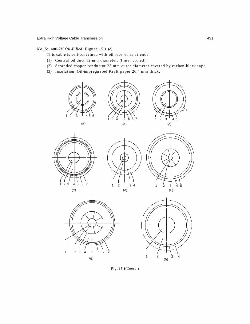
Extra High Voltage Cable Transmission 431
No. 5: 400-kV Oil-Filled. Figure 15.1 (e)This cable is self-contained with oil reservoirs at ends.(1) Central oil duct 12 mm diameter. (Inner cooled).(2) Stranded copper conductor 23 mm outer diameter covered by carbon-black tape.(3) Insulation: Oil-impregnated Kraft paper 26.4 mm thick.
Fig. 15.1(Contd.)
1 2 3 4( )e ( )f
1 2 3 4 5
1 2 3 4 5 6
( )a ( )b ( )c1 2 3 4 5 6 7
1 2 3 4 5 6 7
( )d
1 2 3 4 5
6
1 2 3 4 5 6 7 8
( )g ( )h1 2 3 4

432 Extra High Voltage AC Transmission Engineering
Fig.15.1 Cross-sectional views of typical e.h.v. cables.(a) 69 kV, XLPE;(b) 138 kV oil-filled, self-contained;(c) 275 kV oil-filled, pipe type; (d) 275 kV, XLPE;(e) 400 kV oil-filled, self-contained; (f) 525 kV, HPOF'(g) 500 kV oil-filled, with PPLP composite insulation;(h) 500 kV, XLPE; (i) 1100 kV oil-filled;(j), (k) SF6 gas-insulated line. All cross-sectional views are reasonably to
scale to show comparison of dimensions.
(4) Protection: Lead alloy sheath, metallic reinforcement and PVC jacket of total thickness14.5 mm.
Overall diameter of cable: 105 mm.Oil pressure 200 p.s.i.g. (1.38 MPa).
No. 6: 525 kV HPOF. Figure 15.1 (f)(1) Oil duct : 12 mm inside the conductor.(2) Conductor: 7-segment Milliken type stranded copper 5000 MCM (2500 mm2).(3) Insulation: Oil-impregnated Kraft cellulose paper. 33.8 mm thickness.(4) Sheath: Corrugated aluminium.(5) Jacket: High density polyethylene (HDPE).
No. 7: 500 kV OF Cable with Composite Insulation. Figure 15.1 (g).(1) Oil channel: Inside conductor 25 mm diameter and 1.5 mm thickness. (28 mm total).(2) Conductor: 7-segment Milliken type. Outer diameter 68 mm.(3) Conductor shield: Carbon paper 2 sheets and metallized paper 1 sheet. Total thickness
0.375 mm.(4) Insulation:
mm. 24.5:thicknessTotal
mm4200
mm7m220
mm8m170
mm5.5PPLPthickm120
−
−µ
−µ
−µ
1 2 3 4 5 6( )i
Enclosure EnclosureSF6
Epoxy Epoxy SupportsPost Star Cone
( )j ( )k

Extra High Voltage Cable Transmission 433
(5) Insulation shield: Carbon and metallized papers 0.375 mm.
(6) Copper wire woven with cloth tape 0.5 mm thickness.
(7) Aluminium sheath: 3 mm thickness
(8) Anti-corrosion PVC jacket 6 mm thickness. Overall diameter of cable: 153 mm.
No. 8: 500 kV XLPE. Figure 15.1 (h)(1) Conductor: 2000 mm2 stranded copper with extruded semi-conducting shield.
(2) Insulation: XLPE 35 mm thickness. (Reduced to 32 mm in later design by impregnationwith SF6 gas.)
(3) External shield: Extruded by triple extrusion process along with conductor shield andXLPE insulation.
(4) PVC jacket.
No. 9: 1100 kV Oil-Filled Cable. Figure 15.1 (i)(1) Inner oil duct 24 mm diameter.
(2) Conductor 2000 mm2 area, 57.3 mm outer diameter.
(3) Insulation: Medium density cellulose Kraft paper 35 mm thick.
(4) Lead alloy sheath 6 mm thick.
(5) Reinforcement tapes.
(6) PVC anti-corrosion jacket 6 mm thick.
Overall diameter of cable: 152 mm.Oil pressure: Inner cooled 1.3 MPa.
Outer cooling over jacket with water.
Power transmitted: 3000 MVA 3-phase with only inner cooling.
8000 MVA with both inner oil cooling of conductor and outer water cooling of sheath.
No. 10: Gas Insulated Lines. SF6 gas between 2 to 4 Atmospheres. Figures 15.1 (j) and (k)Maximum voltage, kV: 300 525 765Conductor dia. in mm: 150 250 250Enclosure dia. in mm: 400 600 700Insulation clearance, mm: 125 175 225Gas pressure, atmospheres: 2–4 3–4 3–4
15.1.3 Power Ratings and Environment of CableThe power rating (or, current-carrying capacity for a given voltage level) of a cable dependsvery much on the environment in which the cable is located which determines the heat-disssipation from the outer sheath and the inner conductor. A study carried out by the B.I.C.C.of the U.K. on oil-filled cables for 230 kV, 345 kV, and 525 kV has revealed the following detailsunder several types of environment of the cable. (C.A. Arkell, B. Gregory, G.J. Smee, Trans.IEEE, PAS. 1978, pp. 349-357).
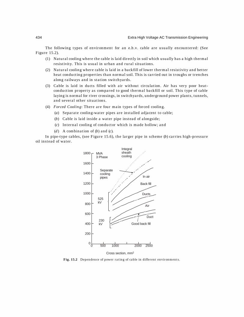
434 Extra High Voltage AC Transmission Engineering
The following types of environment for an e.h.v. cable are usually encountered: (SeeFigure 15.2).
(1) Natural cooling where the cable is laid directly in soil which usually has a high thermalresistivity. This is usual in urban and rural situations.
(2) Natural cooling where cable is laid in a backfill of lower thermal resistivity and betterheat conducting properties than normal soil. This is carried out in troughs or trenchesalong railways and in station switchyards.
(3) Cable is laid in ducts filled with air without circulation. Air has very poor heat-conduction property as compared to good thermal backfill or soil. This type of cablelaying is normal for river crossings, in switchyards, underground power plants, tunnels,and several other situations.
(4) Forced Cooling: There are four main types of forced cooling.
(a) Separate cooling-water pipes are installed adjacent to cable;
(b) Cable is laid inside a water pipe instead of alongside;
(c) Internal cooling of conductor which is made hollow; and
(d) A combination of (b) and (c).In pipe-type cables, (see Figure 15.6), the larger pipe in scheme (b) carries high-pressure
oil instead of water.
Fig. 15.2 Dependence of power rating of cable in different environments.
0 500 1000 2000 2500
Cross section, mm2
200
0
400
600
800
1000
1200
1400
1600
1800
Duct
Good back fill
Air
Ducts
Back fill
In air
Integralsheathcooling
MVA3 Phase
Separatecoolingpipes
525kV
230kV
Extra High Voltage Cable Transmission 435
It has been observed that for a 4000 MCM )mm2000( 2≈ conductor at 525 kV, the following3-phase ratings apply:
(1) With a central oil-duct of 50 mm in diameter—4000 MVA (2.2 A/mm2).
(2) Integral sheath cooling (schem e (b))—1700 MVA (0.935 A/mm2).
(3) Separate cooling pipes adjacent to cable—1500 MVA (0.825 A/mm2).
(4) Cable laid in air with circulation—1300 MVA (0.715 A/mm2).
(5) Cable laid direct in good backfill—1050 MVA (0.578 A/mm2).(6) Cable laid direct in soil of high thermal resistivity or in ducts without air circulation—
900 MVA (0.5 A/mm2).The temperature rise of the conductor is governed entirely by the heats produced in
conductor due to its resistance, the dielectric loss in the insulation, and any heat produced inthe metallic sheath and armouring due to the flow of eddy current. Referring to Figure 15.1, weobserve the following when the presence of armour is neglected:
Let I = current flowing in conductor,R = a.c. resistance of conductor per unit length, cm or m,
Wd = dielectric loss, see equation (15.22) later on, per unit length,λ = ratio of loss in sheath to the I 2R loss of conductor,
T1 = thermal resistance for flow of heat from conductor in the insulation,°C/W-cm or °C/W-m,
T2 = thermal resistance for flow of heat from insulation to sheath,T3 = thermal resistance for flow of heat from sheath to the surrounding
medium in which the cable is laid.Then IEC Standard No. 287 gives the temperature rise of conductor above the ambient,
when any armouring is neglected, to be
θ∆ = )()()( 32121
322
3212 TTTWTTRITTTRI d ++++λ+++ ...(15.1a)
Therefore, the current-carrying capacity of the cable is
I =
2/1
32221
32121
)]()[(
)(
+λ+++
++−θ∆
TTTTTR
TTTWd...(15.1b)
15.2 ELECTRICAL CHARACTERISTICS OF E.H.V. CABLESImportant electrical characteristics that govern the performance of an e.h.v. cable are broadlythe following:
(1) Conductor cross section and radius (or diameter), Ac, rc, or dc;(2) Insulation thickness, ti;(3) Radius (or diameter) to the inside of sheath or outside of insulation, rsh = rc + ti,
(dsh = dc + 2ti);
(4) The ratio ;// cshcsh rrdd =(5) The dielectric constant, or the relative permittivity of the insulation, ;rε
(6) Specific resistivity of insulation, ;iρ
436 Extra High Voltage AC Transmission Engineering
(7) Dielectric loss, Pi;
(8) Loss angle or tan ;iδ
(9) Electric stress in the insulation. Maximum stress Emax; average Eav; and minimumEmin.
(10) Working voltage V at power frequency;
(11) Maximum voltage Vmax at power frequency for the voltage class of cable;
(12) Maximum withstand voltage Vac during dielectric tests at power frequency;);)4to3(( maxac VV ≈
(13) Time duration of application of test voltage Vac, t;
(14) Life expectancy of cable t0, generally in years;
(15) Basic Impulse Level BIL of insulation for the voltage class;
(16) Impulse level of insulation, Vimp, which is used during factory impulse tests. Vimp >BIL by a factor ranging from 1.2 to 2;
(17) Number of shots given during impulse tests;
(18) Volt-tim e withstand or breakdown characteristics called the (V nt = constant) lawbased on probabilistic aspects governed by a Weibull type of distribution for withstandor breakdown voltage (or electric stress) for the insulation structure based onexperiments; (see Section 15.4);
(19) Capacitance per km;
(20) Charging current per km;
(21) Charging kVAR or MVAR per km; and
(22) Partial discharges from voids in dielectric material.As is usual with every type of electrical apparatus or equipment, mechanical and thermal
factors as well as economic factors and technical know-how influence the electrical characteristicsand manufacturing techniques of cables, which are very pronounced at e.h.v. levels. Thus, theconductor temperature, eddy-current loss in metallic parts including the conductor and sheaths,short-circuit current, environment, installation practice, type of cooling, length of cable, bendingand winding on reels and drums, joints and splices, and several other factors peculiar to thecable govern the choice of the most suitable cable for the particular application. We will considerseveral important examples of actual cables used in practice or which are in design anddevelopment stages to illustrate electrical characteristics of cables from an engineering pointof view. A brief description of manufacture of cables will be given in later sections as well asproperties of materials used for the dielectric, which is more a description of material scienceand chemical properties, based on the most advanced techniques to date.
15.2.2 Electrical Stresses in DielectricFigure 15.3 shows the cross-sectional view of a cable with cylindrical central conductor ofradius rc separated from a metallic sheath of radius rsh by a dielectric of thickness ti and relative
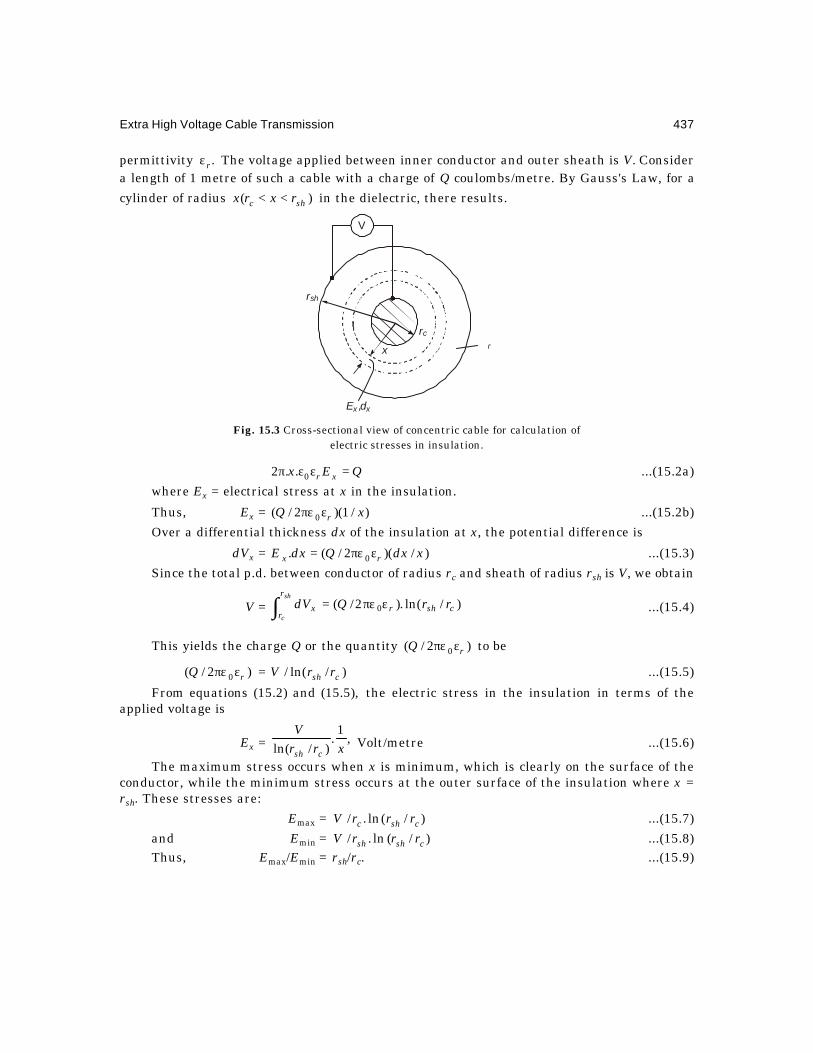
Extra High Voltage Cable Transmission 437
permittivity .rε The voltage applied between inner conductor and outer sheath is V. Considera length of 1 metre of such a cable with a charge of Q coulombs/metre. By Gauss's Law, for a
cylinder of radius )( shc rxrx << in the dielectric, there results.
Fig. 15.3 Cross-sectional view of concentric cable for calculation ofelectric stresses in insulation.
QEx xr =εεπ 0..2 ...(15.2a)
where Ex = electrical stress at x in the insulation.
Thus, Ex = )/1)(2/( 0 xQ rεπε ...(15.2b)
Over a differential thickness dx of the insulation at x, the potential difference is
dVx = )/)(2/(. 0 xdxQdxE rx επε= ...(15.3)
Since the total p.d. between conductor of radius rc and sheath of radius rsh is V, we obtain
V = )/ln().2/( 0 cshr
r
rx rrQdV
sh
c
επε=∫ ...(15.4)
This yields the charge Q or the quantity )2/( 0 rQ επε to be
)2/( 0 rQ επε = )/ln(/ csh rrV ...(15.5)
From equations (15.2) and (15.5), the electric stress in the insulation in terms of theapplied voltage is
Ex = ,1
.)/ln( xrr
V
csh Volt/metre ...(15.6)
The maximum stress occurs when x is minimum, which is clearly on the surface of theconductor, while the minimum stress occurs at the outer surface of the insulation where x =rsh. These stresses are:
Emax = )/(ln./ cshc rrrV ...(15.7)
and Emin = )/(ln./ cshsh rrrV ...(15.8)Thus, Emax/Emin = rsh/rc. ...(15.9)
V
rc
x
rsh
E dx x,
∈r
Fig. 15.3
438 Extra High Voltage AC Transmission Engineering
A large insulation thickness ti yields a large value of ),/1(/ cicsh rtrr += so that theinsulation is not used optimally because the stress eveywhere is not as uniform as it would bewhen rsh/rc is small. In some cable designs, as for example, No. 7 in Section 15.1.2, a materialwith higher withstand stress is used adjacent to the conductor such as thinner paper tape orcomposite insulation (KP or PPLP).
A quantity widely used in design of insulation thickness is the average stress defined byEav = V/ti. In terms of this quantity we obtain
Emax = )/(ln/)./.(av cshci rrrtE
and Emin = )/(ln/)/.(av cshshi rrrtE ...(15.10)
We will now examine numerical values of these electrical stresses for cables with varioustypes of dielectrics and for different e.h.v. levels in order to obtain an idea of average valuesused in practice. These can profitably be used for purposes of comparison before proceeding toother salient electrical characteristics, and to grasp some basic but important properties ofcable designs at e.h.v. levels used all over the world.
Referring back to equation (15.7), for a fixed sheath radius rsh, the maximum stress varieswith the ratio (rsh/rc). There exists a value for this ratio at which the maximum stress can beminimized as follows:
Emax = .)/(ln
1.
1)/(ln c
sh
cshshccsh rr
rrrV
rrrV
=
Let y = ).ln/).(/(thatso),/( max yyrVErr shcsh =
Then,dy
dE max = ,0)(ln
1ln. 2 =
−y
yrV
sh giving
y = rsh/rc = anti loge 1 = 2.7183. (15.11)
If this ratio for sheath radius to conductor radius is maintained by choosing a thicknessfor the dielectric ti = (e – 1) rc = 1.7183 rc, then the resulting electric stress in it at the surfaceof the conductor will be lower than at any other value for ti/rc. Designers aim for this ratio butin practice it cannot be attained in cables for all voltages and insulation thicknesses required.For example, a large conductor cross section in a cable for a given voltage would have a smallerratio for (rsh/rc) than one with a smaller cross section for conductor at the same voltage level.
15.2.3 Examples of Cable Dimensions and Electric StressesTable 15.1 below gives salient dimensions of cables for voltage levels from 69 kV to 1100 kVwith different types of dielectric manufactured in some parts of the world. The electric stressesare also worked out, which the reader should study carefully in order to obtain a good idea ofcable designs for e.h.v. levels, and work them out for herself or himself.

Extra High Voltage Cable Transmission 439
Table 15.1 Dimensions and Electrical Characteristics
Voltage Insulation Cond. Sheath rsh/rc ln ti Stresses* kV/mmClass Type Rad.rc Rad. rsh (rsh/rc) mm Emax Eav Emin
69 kV XLPE 19.3 mm 35.2 mm 1.82 0.6 15.9 3.43 2.5 1.88138 kV 0-F 25.25 38.5 1.525 0.42 16 7.86 5.2 5.15
150 kV EPRM** 13.2 37.5 2.844 1.045 24.3 6.3275 kV HPOF 20 40 2 0.693 19.5 12 8.5 5.36
HPOF 23.5 43 1.83 0.6 19.5
XLPE 20 47 2.35 0.854 27 9.7 6.14 4.13XLPE 23.5 50.5 2.15 0.765
400 kV HPOF 23 49.5 2.15 0.765 26.4 13.8 9.2 6.43500 kV HPOF 34 58.5 1.72 0.543 24.5 17.2 13 10
XLPE 21.1 53.1 2.52 0.923 32 16.3 9.9 6.5765 kV KP-OF 17.9 54.7 3.06 1.12 36.8 22 12 8
PPP-OF 17.9 48.4 2.7 0.995 30.5 24.8 14.5 9.21100 kV HPOF 29 64 2.23 0.8 35 29 19 13
Optimum 2.718 1
15.2.4 Capacitance, Insulation Resistance and Loss Factor tan iδ
From equations (15.4) and (15.5) the capacitance per metre length is, with 0ε = (1000/3π) × 10–12
Farad/metre,
C = F/km),/(ln18/)/(ln/2/ 0 µε=επε= cshrcshr rrrrVQ ...(15.12)
The charging current per phase at frequency f isI = fCVπ2 ...(15.13)
where V = line-to-neutral voltage. This gives a charging reactive power per phase of
Qc = )/(ln/42 0222
cshr rrfVfCVVI εεπ=π= ...(15.14)
We observe that an insulating material with higher relative permittivity rε yields a highercharging power than one with lower rε . It is for this reason that plastic materials XLPE, PPLPand so on are better than oil-filled Kraft paper insulation whose rε 's are on the average 2.3,2.75, and 3.5 respectively. Designers of cable insulation are consequently looking for materialswith low rε and high dielectric strength.
The insulation resistance of the dielectric per metre is
Ri = )/(ln)2/( cshi rrπρ ...(15.15)
*These stresses are calculated at the following maximum working voltages:69 kV 138 kV 275 kV 400 kV 500 kV 765 kV 1100 kV69 145 287 420 550 765 1100
**EPRM—Ethylene Propylene Rubber Moulded.

440 Extra High Voltage AC Transmission Engineering
where iρ = specific resistance in ohm-metre. This equation is derived below as also thefact that the insulation resistance decreases inversely with the length of cable. Thus, longerthe cable lower is its insulation resistance. Referring to Figure 15.4 we observe that the currentin the insulation flows from conductor to sheath since this is the direction of the applied voltageV. At radius x in the dielectric, the area for current flow is )2( xLπ for a cable of axial length L.Consider a cylinder with differential thickness dx at x along the direction of current flow. Itsresistance is
dRi = Lxdxi .2/. πρ ...(15.16)
Fig. 15.4 Calculation of insulation resistance of cable.
The total resistance of the insulation will then be
Ri = ∫ ∫ πρ
=πρ
=sh
c
sh
c
r
r
r
rcsh
iii rr
Lxdx
LdR )/(ln
22 ...(15.17)
showing that ./1 LRi ∝
From equations (15.12) and (15.15), the time constant for decay of any transient appliedbetween conductor and sheath (usually grounded) is
iτ = riiCR εερ= 0 ...(15.18)
Since C varies directly with length of cable L and Ri inversely with L the time constant iτis independent of L. However, the propagation delay of a transient such as lightning through acable depends on cable length.
The surge impedance of the cable is
Zc = 1/v C ...(15.19)
where v = velocity of propagation of surge
= ,/103/1 800 rr ε×=εεµ metres/second. ...(15.20)
∴ Zc =
εε
µπ
=επεεεµc
sh
rrcshr r
rrr ln21
2/)/(ln0
0000
= ./)/(ln60 rcsh rr ε ...(15.21)
rcx
rsh
dx
L
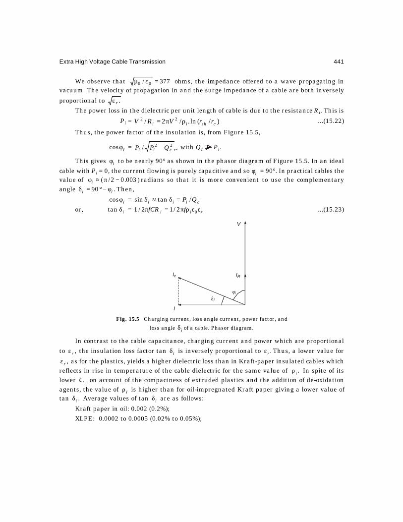
Extra High Voltage Cable Transmission 441
We observe that 377/ 00 =εµ ohms, the impedance offered to a wave propagating invacuum. The velocity of propagation in and the surge impedance of a cable are both inversely
proportional to .rεThe power loss in the dielectric per unit length of cable is due to the resistance Ri. This is
Pi = )/(ln./2/ 22cshii rrVRV ρπ= ...(15.22)
Thus, the power factor of the insulation is, from Figure 15.5,
iφcos = ,./ 22cii QPP + with Qc Pi.
This gives iφ to be nearly 90° as shown in the phasor diagram of Figure 15.5. In an ideal
cable with Pi = 0, the current flowing is purely capacitive and so iφ = 90°. In practical cables thevalue of )003.02/( −π≈φi radians so that it is more convenient to use the complementaryangle .90 ii φ−°=δ Then,
iφcos = ciii QP /tansin =δ≈δor, iδtan = rii ffCR εερπ=π 02/12/1 ...(15.23)
Fig. 15.5 Charging current, loss angle current, power factor, and
loss angle iδ of a cable. Phasor diagram.
In contrast to the cable capacitance, charging current and power which are proportional
to ,rε the insulation loss factor tan iδ is inversely proportional to .rε Thus, a lower value for
,rε as for the plastics, yields a higher dielectric loss than in Kraft-paper insulated cables whichreflects in rise in temperature of the cable dielectric for the same value of .iρ In spite of itslower ,rε on account of the compactness of extruded plastics and the addition of de-oxidationagents, the value of iρ is higher than for oil-impregnated Kraft paper giving a lower value oftan .iδ Average values of tan iδ are as follows:
Kraft paper in oil: 0.002 (0.2%);
XLPE: 0.0002 to 0.0005 (0.02% to 0.05%);
V
Ic
I
IR
δi
φi

442 Extra High Voltage AC Transmission Engineering
Composite PPLP: 0.0007 (0.07%);
SF6: 0.
Table 15.2 shows values of capacitance, charging current, and MVAR of some typicalcable designs used in practice.
Table 15.2. C, I, Qc of Some Typical Cable Designs
Qc
Type and Voltage In (rsh/rc) C, µ F/km I, A/km MVAR MVARkm-ph km-3-ph
Category I: HPOF C= 3.6/18 ln (rsh/rc)138 kV (145 kV Maximum) 0.422 0.46 12.12 1.015 3.045
275 kV (287 kV) 0.693 0.28 14.5 2.314 6.942500 kV (550 kV) 0.5427 0.358 35.74 11.35 341100 kV (1150 kV) 0.8 0.246 51.3 34 102
Category 2: XLPE C = 2.3/18 ln (rsh/rc)275 kV (287 kV) 0.854 0.15 7.89 1.29 3.87500 kV (550 kV) 0.923 0.1384 13.8 4.39 13.17Category 3: PPLP C = 2.7/18 ln (rsh/rc)
765 kV (765 kV) 0.995 0.1508 20.925 9.38 28.14
From the information provided in Tables 15.1 and 15.2, the reader might have observedmany of the salient properties of cables and their insulation as used in practice. A summary ofsalient points is worth noting in order to effect a comparison between O-F cables, XLPE cablesand PPLP (oil filled) cables, which now consist all e.h.v. cables manufactured with solid insulation.
275 kV 500 kV 765 kV 1100 kV rsh/rcHPOF ti = 19.5 mm 24.5 mm 35 mm 1.72–2.23PPLP ti = 30 mmXLPE ti = 27 mm 32-35 mm 2.15–2.52
(1) XLPE cables have higher (rsh/rc)-ratio than HPOF cables.
(2) XLPE cables have larger insulation thickness than HPOF cables.The difference is 7.5 to 10 mm in 275 kV and 500 kV cables.
(3) XLPE cable has a lower charging current than HPOF cable in the ratio of nearly 2 to1. (Table 15.2).
(4) Average electric stress (Eav = V/ti) in the insulation for power frequency is as followsat maximum working voltages:
275 kV (287 500 kV 765 kV 1100 kVkV maxm.) (550 kV) (1150 kV)
HPOF 8.5 kV/mm 13 14 19= MV/m
XLPE 6.1 10 — —

Extra High Voltage Cable Transmission 443
(5) Maximum values of electric stress Emax = Eav (ti/rc)/ ln (rsh/rc) for power frequency atmaximum working voltages are as follows:
275 kV 500 kV 765 kV 1100 kVHPOF 12 17.2 22–25 29XLPE 9.7 16.3 — —
Example 15.1 The oil pressure in a HPOF cable is 1 MPa (Mega Pascal). Calculate thepressure in (a) Lbs/in2; (b) Atmospheres; (c) Lbs/in2-gauge; (d) kg/cm2.
Solution.1 Pascal = 1 Newton/sq.m.
1 Newton = force required to accelerate 1 kg by 1 m/s2;1 Lb = force required to accelerate 1 Lb by 32.2 ft/s2
= 0.454 kg × 32.2/3.28 m/s2 = 0.454 × 9.81 = 4.457 N.(a) ∴ 1 MPa = 106/(4.457 × 39.362) = 144.83 Lbs/in2.(b) 1 Atmosphere = 14.7 Lbs/in2. ∴ 1 MPa = 9.8524 Atm.;(c) 1 MPa = 144.83 Lbs/in2 = 130.13 Lbs/in2 – gauge,(d) 1 kg/cm2 = 2.542/0.454 Lbs/in2 = 14.21 Lbs/in2 (≈ 1 Atm.)
∴ 1 MPa = 10.192 kg/cm2.Note : Normal oil pressure used in HPOF cables ranges from 100 to 250 Lbs/in2, or, 0.69
to 1.725 MPa.
Example 15.2. An XLPE cable for 275 kV work is rated as follows:(i) Maximum working voltage of 287 kV, line-to-ine;
(ii) 805 kV (line-to-neutral) withstand for 1 hour at ambient temperature (50 Hz voltage);
(iii) 735 kV (l-to-n) 50 Hz withstand for 1 hour at 90°C for conductor temperature; and
(iv) 1590 kV peak (l-to-n) lightning impulse voltage of 1.2/50 sµ double-exponential shape.Other details are: rε = 2.3 for XLPE; ti = 27 mm thickness for the insulation, conductor
radius rc = 23.5 mm f = 50 Hz.
Calculate the following quantities:(a) Average electric stress in the insulation at the maximum working voltage, test voltages
of 735 kV and 805 kV, and 1590 kV impulse.
(b) Emax and Emin in the insulation at 287 kV (l-to-l ) and 805 kV (l-to-n) at power frequency;
(c) Velocity of propagation of lightning surge in the cable;
(d) The surge impedance, Zc;
(e) Capacitance, charging current and MVAR at maximum working voltage per km ofcable in service;
(f) The transformer capacity for testing the cable at 805 kV;
(g) If tan iδ = 0.0005, calculate the dielectric loss and insulation resistance per km, andthe specific resistivity of the dielectric;
(h) Assume that the quantity V 2t = constant and V = 805 kV (l-to-n) for t = 1 hour.Calculate the life of the cable t0 in years when V = 287 kV (l-to-l);

444 Extra High Voltage AC Transmission Engineering
(i) Using 735 kV (l-to-n) and t = 1 hour at the elevated temperature of 90°C, determinethe life of the cable in years if it is operated continuously at this temperature insteadof at room temperature.
Solution.
(a) V = kV/mm.14.627/7.165.,kV3/287,kV287 av ==∴−=− Enlll
V = kV/mm.8.2927/805.,kV805 av ==∴− Enl
V = kV/mm.22.2727/735.,kV735 av ==∴− EnlV = kV/mm.9.5827/1590.,kV1590 av ==∴− Enl
Note that for power frequency the average stress at maximum value of voltage used inthe 1-hour test is 30 kV/mm while it is 60 kV/mm under impulse condition. This is for XLPEinsulation.
(b) Sheath radius rsh = 23.5 + 27 = 50.5 mm. ∴ ln (rsh/rc) = 0.765.At 287 kV, l–l = 165.7 kV, l–n, Emax = V/rc. ln (rsh/rc) = 9.22 kV/mm,
At 805 kV, l–n, Emax = 44.8 kV/mm ≈ 1.5 Eav.At 287 kV, l–l, Emin = Emax.rc/rsh = 4.29 kV/mm.
At 805 kV, l–n, Emin = 20.85 kV/mm.
(c) v = rεεµ 00/1 = 3.2/103 8× = 1.98 × 10⁸ m/s = 66% of light velocity.
(d) Zc = 6.2483.2/377 = ohms
(e) C = )/ln(/2 0 cshr rrεπε = 765.018/3.210 9 ××−
= 0.167 nF/m = 0.167 µF/km.
Charging current, I = 314 × 0.167 × 10–6 × 165.7 × 103 = 8.69 A/km. Qc = 8.69 × 165.7 = 1440kVAR/phase = 4.32 MVAR/3-phase per km.
(f) At 805 kV and 1 km of cable, charging current = 314 × 0.167 × 10–6 × 805 ×103 = 42.23Amp.
∴ Capacity of transformer should be at least 805 kV and 42.23 Amp. and 34 MVA. Suchlarge transformers for testing purposes are not normally available so that only shorterlengths of cable must be used during factory or laboratory tests. It is alo usual toprovide research factors of 1.3 for such transformers.
(g) Dielectric loss: Pi = Qc tan iδ = 4.32 × 103 × 0.0005 = 2.16 kW/km-3 phase.
tan .2/1/ icii fCRQP π==δ
∴ 14.38)0005.010167.0314/(1 6 =×××= −iR Megohms/km.
Also, tan .2/12/1 0 riii ffCR εερπ=π=δ
∴ ρi =ir
ir ff
δε×π×π=δεεπ
− tan10)36/1000(2
1)tan2/(1
120
= )0005.03.2100050/(1018 12 ××××= 1210313.0 × ohm-metre.

Extra High Voltage Cable Transmission 445
(h) Since V 9t = constant, at 805 kV for 1 hour test, there is
1)10805( 93 ×× = life.93 )107.165( t××
0life tt =∴ = years.172hours)7.165/805( 9 =
(i) At the elevated temperature, life of cable is
t0 = 7624365
17.165
7359
=×
×
years.
15.3 PROPERTIES OF CABLE-INSULATION MATERIALSMaterials used for insulation in e.h.v. cables are:
(1) Oil-impegnated Kraft cellulose paper. The oil used is either mineral or mostly syntheticof low viscosity;
(2) Extruded rubber or plastic, chiefly Ethylene Propylene Rubber (EPR), Polyolefin groupthe most important of which are Cross-Linked Polyethylene (XLPE) and Polypropylene(PP);
(3) Composite insulation consisting of paper and plastic films. These have the chemicalnames such as Kraft-XLPE, Kraft-PP also called PPLP, Polymethyl Penteen (PML),and non-polyolefin group consisting of Fluorinated Ethylene-Propylene copolymers(FEP/C) in which a Fluorine molecule replaces Hydrogen of Polyethylene (PE);
(4) Gas. This is mainly Sulphur Hexafluoride, SF6.
Each type offers certain advantages and disadvantages when used for e.h.v. applicationsfor cables. We shall enumerate the chemical, electrical, thermal and mechanical propertiesvery briefly of the above materials in so far as they concern cable insulation. The literature onthese materials is so extensive that the reader is strongly urged to follow it from other sources.
15.3.1 Oil-Filled Paper Insulated CablesThe OF cable has highest dielectric strength of all types of insulated cables. Voltages of OFcables have increased utp 1200 kV. There are three main types of OF cables; (1) The pipe-typeHPOF cable used mainly in the U.S.A.; (2) Flat-type or Mullehöj cable of Denmark and usedearlier; and (3) Low-pressure OF cable. There are several variations of these, the most importantbeing the self-contained HPOF variety.
The paper used is Kraft cellulose paper, de-ionized and water-washed during manufacture.Unimpregnated Kraft paper has a specific gravity of 1.5 and relative permittivity .5.5=ε r
These properties give rise to high dielectric loss, high capacitance, high charging current, andmoreover it is hygroscopic. But when impregnated with low-viscosity, low-density syntheticoils composed mainly of alkyl benzene and hydrogenated polybutene oil (DDB ) and some mineral
oils the permittivity falls to 4.3=ε r and a loss angle tan iδ =0.002 (0.2%). When plastic films
are used along with Kraft paper and with improvements taking place in oil properties, as of
1986, for 765 kV cables already manufactured, 7.2=ε r and tan %.07.0=δi The paper for such
application is made of low density which normally absorbs moisture easier than high densitypaper. But when impregnated with oil, it exhibits high impermeability to moisture.

446 Extra High Voltage AC Transmission Engineering
The chief disadvantage of this type of insulation is the differential expansion betweenpaper and metallic conductor so that during load cycling especially during cooling, voids arecreated. This is avoided by using high oil pressure (> 200 p.s.i. = 1.38 MPa). High pressure OFcables with both internal cooling of conductor and external cooling of sheath has resulted incables suitable upto 1100 kV, 8000 MVA, 3-phase.
The impulse strength of paper cables is a limiting factor in their design. Higher density ofpaper and higher viscosity of impregnant yield higher impulse strength. But this results inhigher rε which increases dielectric loss, capacitance and so gives rise to higher insulationtemperature and charging current. This shows that increasing the permittivity also increasesimpulse strength, but the increased temperature gives rise to thermal instability (run-awaycondition). These are minimized with laminated polypropylene film (PPLP) as will be discussedlater on.
Usual paper thickness is 5–6 mils (0.127–0.1524 mm), but 3-mil paper is used for innerlayers near the conductor. The thickness of paper is related to the dielectric strength; thethinner it is the higher the kV/mm it can stand. In cables operating at extremely high stresses0.75-mil paper has also been used. A paper with lower density gives lower power factor, lossesand lower charging current, but because of loose packing of molecules and fibres, allows gas topermeate easily which affects the electric strength. Thus, electric strength and dielectric lossact in opposite directions, lowering of dielectric loss is accompanied by weakness of dielectricproperties.
The cross section of a 3-phase pipe-type cable is shown in Figure 15.6. The high oil pressureused (1.5–1.7 MPa) not only is effective in removing heat but also prevents formation of voids inthe insulation and therefore partial discharges (coronas) as well as preventing moisture ingress.
Fig. 15.6 Cross section of typical 3-phase pipe-type oil-filled cable.
Self-Contained Oil-Filled CablesThe self-contained OF cable has no pipe in which the three single-core cables are laid but onlyan oil duct inside the conductor. This is preferred when the cable has to be laid in an inclined orvertical direction as in shafts. The advantages over pipe-type cables are as follows:
(a) Smaller conductor cross section due to better cooling since the 3 single-core cablescan be laid with any distance of separation unlike in a pipe. Sheath power losses canbe minimized by proper bonding of cables.
Pipe withPressure Oil

Extra High Voltage Cable Transmission 447
(b) Due to disturbances caused during laying, pipe-type cables require larger insulationthickness than self-contained OF cables.
(c) No pumps are necessary. Only oil tanks are sufficient.
(d) Obstacles can be jumped easier than with heavy pipes.
(e) Self-contained OF cables are cheaper than pipe-type cables.
(f) When a damage occurs to pipe-type cable, all 3-phases are removed out of service.
(g) In sites where laying conditions are severe, self-contained OF cables are preferred ashas been the experience in giant power stations, such as the Grand Coulee Dam inthe U.S.A.
A cross section of 400-kV self-contained OF cable is shown in Figure 15.1(e) having 8components (See p. 431):
(1) Oil duct 12 mm diameter; (2) 9-segment copper conductor 300 mm2 area; (3) Internalshielding; (4) Insulation 26.4 mm thick; (5) External shielding; (6) Lead-alloy sheath; (7) Bronzereinforcement; and (8) PVC jacket.
Many undersea dc cables in the world also use the self-contained OF system. Some examplesare:
(1) Gotland—Sweden Link— ± 100 kV, 20 MW;(2) France—England Link— ± 100 kV, 160 MW; ± 270 kV, 2000 MW;(3) Vancouver Island, Canada— ± 300 kV, 500 MW;(4) Skagerrak Strait— ± 250 kV, 500 MW.
Other dc cable installations exist in Italy–Sardinia, North and South Islands of New Zealand,and several other places.
Average electrical stresses used in HPOF cables have been given in Table 15.1 for powerfrequency at maximum voltages used at a specified voltage level. However, design stresses areusually higher than at working voltages when the cables are to be tested at the factory. Thesetest voltages are agreed between manufacturer and buyer so that they do not represent standardvalues.
Power Frequency Impulse
275 kV: ti = 19.5 mm 41 kV/mm (805 kV test) 81 kV/mm (1590 kV test)
400 kV: ti = 26.4 mm 31 kV/mm (830 kV) 56 kV/mm (1475 kV)500 kV: ti = 24.5 mm 44 kV/mm (1087 kV) 92 kV/mm (2250 kV)765 kv: ti = 30.5 mm 55.3 kV/mm (1150 kV) 144 kV/mm (3000 kV)
15.3.2 Cross-Linked Polyethylene Cables—XLPEThe search for an insulating material with low relative permittivity, low dielectric loss, highelectric strength, without the necessity for an oil or impregnating fluid, easy installation, betterfire-resistant property, and attack against chemicals has resulted in the design of cables withcross-linked polyethylene, XLPE, as insulation. As of now this material has been utilized upto500 kV in cables used extensively in Europe and Japan although they are used all over theworld to greater or less extent.
Polyethylene (PE) is a hydrocarbon thermoplastic material which by itself is a good insulant.It is obtained by using ethylene gas, a by-product of coal, and was invented by I.C.I. in the U.K

448 Extra High Voltage AC Transmission Engineering
prior to the 1939-45 war. Its molecular representation is .)|
|
|
|( 22 nCHCH −−− It has a softening
point of 70°C and melting point of 115°C, a specific gravity of 0.9–1.0, high breakdown strengthof 60 kV/mm, low tan iδ of 0.0002 to 0.0005, low dielectric constant of 2.2–2.5, high insulationresistivity, low thermal resistance of 30°C–cm/watt, and resists attack by chemicals, both acidsand alkalis. Normally the maximum operating temperature of conductor used in cables is 80°Cbut 90°C is allowed. The main disadvantage of PE is its vulnerability for being affected bypartial discharges in the presence of moisture.
The hydrogen molecule in PE gives undesirable properties such as easy attack from oxygenin moisture. In cross-linking, many bonds between C and H2 are removed, resulting in morebonds between carbon atoms. The resulting material is Cross-Linked Polyethylene, XLPE. Itsdensity increases to 0.94 to 0.96 because of removal of lighter hydrogen. Its other properties are
rε = 2.25 to 2.35, tan iδ = 0.05%. The molecular chain is represented as .)|
|
|
|
|
|( 22 nCH
C
C
C
CH −−−−
The amount of cross-linked carbon bonds usually varies between 7 and 10% of the total bonds,but this is sufficient to yield insulating properties superior to normal High Density Polyethylene(HDPE, 0.95 gm/cc) and Low Density Polyethylene (LDPE, 0.92 gm/cc). HDPE is used forprotective jackets over the cable in place of PVC. XLPE has an impulse breakdown strength of400 kV/mm at 90°C which falls to 200 kV/mm at 130°C due entirely to the loss of crystalstructure at the elevated temperature. At room temperature it increases to 450 kV/mm givingthe temperature coefficient
K1 = .125.1400450
temp.cond.maxm.atstressBreakdownetemperaturroomatstressBreakdown
==
This is an important factor in design of cable-insulation thickness. In comparison, LDPEof 0.92 gm/cc has an impulse breakdown strength of 400 kV/mm at 90°C and HDPE of 0.95 gm/cc gives 520 kV/mm. But as has been pointed out earlier, higher density gives higher dielectricloss and charging current while also being more stiff and less flexible to handle than XLPE.Lower density is more permeable to moisture. Thus, XLPE is a good compromise betweenHDPE and LDPE.
The reader should refer to literature on Polymer Science for details of manufacture ofthis material. A short description of the cross-linking process is given here. There are essentiallythree types of processes.
(1) Chemical Cross-Linking: Here, a compound of LDPE and some peroxide reagent ascatalyst are used. At about 250°C, the free ethylene radicals (CH2) react with eachother in the presence of the catalyst to form a vulcanized or cross-linked materialunder high temperature and pressure.
(2) Nuclear Irradiation: This is a very expensive process and is used for insulation inspecial applications such as in nuclear plants themselves. The plastic material is

Extra High Voltage Cable Transmission 449
bombarded in an atomic pile or nuclear reactor by thermal neutrons. A high-energybeam of electrons produced in an accelerator is also used commercially. This gives aproper doze of irradiation to the finished PE cable.
(3) Vulcanizing: The manufactured cable with extruded PE material on the metallicconductor is passed through a vulcanizing tube. In the old process (discontinued now)this was done under steam which introduced microvoids so that dry curing process isused at present in cable manufacture. The heating under high pressure is carried outin an atmosphere of Nitrogen or other insert gas. Other processes use Silicone oil,salt baths, or by imparting energy required for cross-linking through ultra-sonic waves.Some laser techniques are under development. The process of cross-linking wasintroduced by the General Electric Co. of U.S.A. in 1953, but XLPE cables have foundmore widespread use outside U.S.A.
The high quality of XLPE cables is a product of improved design and manufacturingtechniques and processes, chief among which are:
(a) Assuring uniformity in insulation;(b) Reduction of voids, contaminants and moisture content. Contaminants include metallic
particles, fibrous materials and other impurities;
(c) Improved adhesion and smotth surface at the interface between insulation and semi-conducting layer on the conductor as well as the inner surface of the sheath.
Fig. 15.7 Schematic diagram of cross-linking process of XLPE.
These have resulted from the following processes:
(i) The dry curing process which is shown schematically in Figure 15.7;(ii) Triple co-extrusion process where the semi-conducting layers and the resin making
up the XLPE insulation are extruded together in a specially-shaped nipple die; and
(iii) Selecting extra pure materials (resins) by strict quality control methods to excludecontaminants and voids, and using highly sophisticated methods of packing duringtransportation from resin manufacturer to the cable factory.
The ultimate aim is to reduce the insulation thickness which at present is 10 mm thickerthan in HPOF cables for the same voltage. As mentioned before, XLPE should not lose its
N gas out2 N gas in2 out inHeaters Water
Heating Zone Cooling ZonePre-cooling
Zone
PackingPacking
Cable

450 Extra High Voltage AC Transmission Engineering
crystalline structure and become amorphous if its impulse strength is to be preserved and notdegraded badly with rise in temperature. However, the ac breakdown strength is not affectedby the loss of crystallinity or change in density.
Fig. 15.8 Illustrating water-tree formation in XLPE,
The cause for breakdown of XLPE insulation is "water treeing" and "bow-tie treeing",reported first by Lawson and Vohlstrom in 1973. These are due to a combination of electricaland mechanical stresses, moisture ingress, and temperature as well as the presence ofcontaminants, voids and protrusions. The actual mechanism of water-tree initiation and growthare still improperly understood. There exist several theories the main one being related to theelectric charge accumulated in the XLPE. Figure 15.8 shows a picture of a water tree wherebubbles or voids are formed along the dielectric lines of force, which are radial in a concentriccylindrical electrode system. Water-tree resistant materials are used to combat this and areknown as "voltage stabilizers" or electrolytes. Such additives are compounds having names likeFerrocene, 8-Hydroxyquinoline and Siloxane oligomer. These are polymers of ethylene.Figure 15.9 shows an example of number of water trees in 5 mm thickness of insulation withdifferent lengths of trees in XLPE with and without these "stabilizers". No trees over 240
mµ (0.24 mm) are formed with additives. It is believed that water trees are initiated at theinterface of the shield, wrapped on the conductor, and the XLPE insulation. If this interface ismade perfectly smooth and cylindrical, water-tree formation due to any absorption of moistureis difficult to initiate. This is why the triple-extrusion process assumes great importance. Water-tree resistant XLPE is known as WTR-XLPE. Any method used for measuring the charge inthe insulation is a valid diagnostic procedure for predicting water-tree formation and consequentdeterioration of the insulation. A partial discharge level of 100 pC is generally considered theupper limit for good insulation.
Fig. 15.9 Typical illustration of number of water trees and their length in XLPE cableswith and without additives.
10
5
0 80 100 200 280
No.
of
tree
s in
5 m
m Without additives
WTR-XLPE with voltage stabilizer
Length of Trees, mµ

Extra High Voltage Cable Transmission 451
Due to constant improvements, the voltage of XLPE cables has reached 500 kV (550 kVmaximum), the continuous working electric stress has increased from 5 kV/mm for 66-kVcables to 10 kV/mm for 500 kV cables. Insulation thicknesses have increased from 10 mm at 66kV to 32-35 mm at 500 kV.
Bow-tie trees are generated from microvoids or contaminants in the insulation, and arepresent even in dry-cured (radiant curing process for cross-linking) XLPE cables if worked athigh temperature in a humid atmosphere or under water. Therefore, a water-impermeablemetal sheath is usually adopted or else a water-proof layer under the anti-corrosion PVC jacketis given. WTR-XLPE is also less susceptible to bow-tie tree formation. The water-proof layerusually consists of a thin lead or other metallaminated plastic tape applied over the insulationor below the PVC jacket. The number of trees is thereby decreased to below 1 per cc and theirlength does not exceed 0.15 mm. On the other hand, normal XLPE develops 100/mm3 and thelength can exceed 0.25 mm (250 m).µ
The following values of maximum electrical stresses are found in XLPE cables. (See alsoTable 15.1).
Voltage Insulation Power Frequency Impulse(Maximum) thickness, ti
275 kV (287 kV) 27 mm 30 kV/mm (805 kV) 59 kV/mm (1590 kV)
500 kV (550 kV) 32 mm 34 kV/mm (1087 kV) 70 kV/mm (2250 kV)
As compared to this, OF paper cable takes higher electrical stresse. For power frequencyit is higher by 10 kV/mm and for impulse by 20 kV/mm.
15.3.3 Composite Laminated InsulationDetails of a 500 kV and 765 kV OF cable with composite insulation were given in Section 15.1.1,and Figure 15.1(g). The insulation consisted of PPLP and PML (Polypropylene Laminated KraftPaper and Polymethyl Pentene Laminated Kraft Paper). XLPE-laminated paper is also used.Impregnated Kraft paper has rε = 3.5 while XLPE has rε = 2.3. A laminated Kraft paper andplastic film has rε = 2.7. tan iδ values are also intermediate between the two with 0.0007 to0.001. The plastic films are laminated with paper on both sides by chemical bonding or byextrusion. The ratio of plastic/paper governs kV/mm, ,rε and tan .iδ For lowering the dielectricloss, the plastic content is increased. Normal ratio of plastic/paper is 40/60%. For a 500 kVcable, 25 mm thickness for laminated insulation is sufficient which is the same as for paper-insulated cables whereas a thickness of 33 mm is necessary for XLPE insulation.
The electric stresses used during high-voltage tests on a 500-kV cable are as follows:Power Frequency—840 kV test, Eac = 45 kV/mm, maximum;Lightning Impulse—2360 kV test, Eimp = 130 kV/mm, peak.Some of the laminated papers and their details are shown below (See Figure 15.10 for
sketch):
Polyolefin Group(1) Kraft-XLPE: Density—0.94 to 0.96 gm/cc
Melting point—130°C

452 Extra High Voltage AC Transmission Engineering
Fig. 15.10 Laminated Kraft paper and plastic films for composite insulation in cables.
rε = 2.25 to 2.35 (for power frequency)
tan %05.0<δi
Lamination by extrusion.
formsheetinstressBreakdownkV/mm260:StressImp.
kV/mm120:StressAC
=
=
B
B
E
E
(2) Kraft-Polypropylene:
n
—CH—
—CH—CH—
3
2
Density—0.91 gm/ccMelting point—170°C
%03.0tan,25.2 <δ=ε ir
Laminated by extrusion
formsheetInkV/mm250:Stress Imp.
kV/mm135:StressAC
=
=
B
B
E
E
(3) Kraft-Polymethyl Penteen (TPX). Also PMLP:
—CH —2 CH—|CH|
2
–—CH—–|CH3
|CH3 n
Density–0.83 gm/ccMelting point—235°C
%03.0tan,1.2 <δ=ε ir
formsheetIn kV/mm245 :StressImp.
kV/mm116:StressAC
=
=
B
B
E
E
KP
KP
XLPEPP
TPX
Extra High Voltage Cable Transmission 453
PMLP has higher melting point than KP-XLPE and KP-PP so that it may be used adjacentto the conductor. In a 500-kV cable the 25 mm thickness is made up of 4 mm of PMLP adjacentto the conductor and 21 mm of PPLP on top of the PMLP.
For making the cable impervious to moisture, a metal such as Pb, Al, or Cu in foil form isused which is about 50 to 100 mµ (0.05 to 0.1 mm) thin. This is sandwiched between two layersof plastic films each of 100 mµ thickness. Such a composite tape is 250 to 300 mµ (0.25 to 0.3mm) thick. The water-impervious layer eliminates bow-tie tree formation in the cable nearlycompletely.
15.4 BREAKDOWN AND WITHSTAND ELECTRICAL STRESSES IN SOLIDINSULATION—STATISTICAL PROCEDURE
In Chapter 11, breakdown and withstand voltages of a long airgap with several electrodegeometries were discussed such as conductor-tower, rod-plane, etc. These were done fromstatistical considerations. For long airgaps, the 50% breakdown voltage was an important quantity.The problem was to ascertain the withstand voltage from experimental results of breakdownvoltages, and it was mentioned there that the accepted value of withstand voltage is %50)31( ×σ−Flashover Voltage or Critical Flashover Voltage (C.F.O.), where σ = standard deviation. Thisvalue of "withstand voltage" actually gives a probability of 0.2% breakdown when the probabilitydistribution of breakdown follows a Gaussian distribution. Ideas similar to these are applied tobreakdown and withstand voltages and electrical stress of solid insulations used in cables,transformers, etc. The problem is always the following: By performing a set of tests extendingover a short period of time (a few hours at most) in a laboratory and factory, can we predict thelong-duration (theoretically infinite time but 30 to 50 years in practice) performance of theinsulation structure? In this connection, we will encounter the Volt-Time (V–t) characteristicsof the insulation structure at a given voltage (or electric stress) following the Weibull distributioninstead of the Gaussian or Normal.
15.4.1 The Weibull Probability Function for Breakdown GradientFrom a vast experience gained with breakdown characteristics of solid insulation structures ofmany types and between electrodes of many geometries, it has been established that theprobability of breakdown at a certain level of voltage gradient or electric stress in the insulationis given very well by the following functional relationship :)1)(0 ≤≤ EP
P(E) = bL EEE /)(exp1 0−−− ...(15.24)*
where P(E) = fractional probability of breakdown of the insulation structure at agiven electric stress E,
E = electric stressEL = maximum withstand electric stress, or the least stress for
commencement of breakdown,E0 = a scale factor having units of electric stress,
and b = breakdown exponent.
* In the original paper of Weibull (Ref. 41 under Other Journals) the probability function is taken as F(x)= 1–exp–(x–x0)m/x0. With x0 and m constant, the expression is equivalent to (15.24).
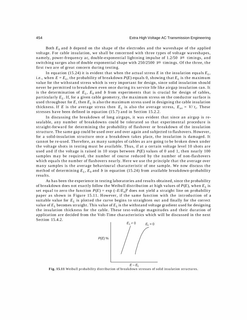
454 Extra High Voltage AC Transmission Engineering
Both E0 and b depend on the shape of the electrodes and the waveshape of the appliedvoltage. For cable insulation, we shall be concerned with three types of voltage waveshapes,namely, power-frequency ac, double-exponential lightning impulse of 1.2/50 sµ timings, andswitching surges also of double exponential shape with 250/2500 sµ timings. Of the three, thefirst two are of great concern during testing.
In equation (15.24) it is evident that when the actual stress E in the insulation equals EL,i.e., when E = EL, the probability of breakdown P(E) equals 0, showing that EL is the maximumvalue for the withstand stress which is very important for design, since solid insulation shouldnever be permitted to breakdown even once during its service life like airgap insulation can. Itis the determination of EL, E0 and b from experiments that is crucial for design of cables,particularly EL. If, for a given cable geometry, the maximum stress on the conductor surface isused throughout for E, then EL is also the maximum stress used in designing the cable insulationthickness. If E is the average stress then EL is also the average stress, Eav = V/ti. Thesestresses have been defined in equation (15.7) and in Section 15.2.2.
In discussing the breakdown of long airgaps, it was evident that since an airgap is re-sealable, any number of breakdowns could be tolerated so that experimental procedure isstraight-forward for determining the probability of flashover or breakdown of the insulationstructure. The same gap could be used over and over again and subjected to flashovers. However,for a solid-insulation structure once a breakdown takes place, the insulation is damaged. Itcannot be re-used. Therefore, as many samples of cables as are going to be broken down underthe voltage shots in testing must be available. Thus, if at a certain voltage level 10 shots areused and if the voltage is raised in 10 steps between P(E) values of 0 and 1, then nearly 100samples may be required, the number of course reduced by the number of non-flashoverswhich equals the number of flashovers nearly. Here we use the principle that the average overmany samples is the average behavioural characteristic of one sample. We now discuss themethod of determining EL, E0 and b in equation (15.24) from available breakdown-probabilityresults.
As has been the experience in testing laboratories and results obtained, since the probabilityof breakdown does not exactly follow the Weibull distribution at high values of P(E), when EL isset equal to zero the function P(E) = exp (–E/E0)b does not yield a straight line on probabilitypaper as shown in Figure 15.11. However, if the same function with the introduction of asuitable value for EL is plotted the curve begins to straighten out and finally for the correctvalue of EL becomes straight. This value of EL is the withstand voltage gradient used for designingthe insulation thickness for the cable. These test-voltage magnitudes and their duration ofapplication are decided from the Volt-Time characteristics which will be discussed in the nextSection 15.4.2.
Fig. 15.11 Weibull probability distribution of breakdown stresses of solid insulation structures.
EL = 0EL 0≠
P E( ) %
E – EL
Extra High Voltage Cable Transmission 455
Reverting to equation (15.24), we observe that there are three unknowns (EL, E0, and b) tobe determined from experimental values. Therefore, we require three sets of known values forP and E. We might also observe that.
]ln)([ln1
1lnln 0EEEb
P L −−=
− ...(15.25)
This shows that a straight line results on a probability paper where the ordinate is m = ln
− P11
ln and the abscissa is ln (E – EL). It is then easy to find the value of b graphically since
the slope of the straight line is b. We shall now set forth an analytical procedure in order to findEL, E0, and b. Let the probabilities of breakdown be P1, P2, P3 at voltage gradients E1, E2, and E3which are obtained from experiments. The gradients are of course calculated from the breakdownvoltages. Then we have:
and
−−=−=−−=−=
−−=−=
]ln)([ln)]1/(1[lnln
]ln)([ln)]1/(1[lnln
]ln)([ln)]1/(1[lnln
0333
0222
0111
EEEbPmEEEbPm
EEEbPm
L
L
L
...(15.26)
Eliminating b and E0, there results
)(ln)(ln)(ln)(ln
23
12
23
12
LL
LL
EEEEEEEE
mmmm
−−−−−−
=−−
...(15.27)
This equation can be solved by trial and error for EL, the electric gradient at initialbreakdown or the maximum value of withstand voltage. Having determined this, the values ofexponent b and scale factor E0 can be calculated from any two of the three equations in (15.26),thus:
b = )/()(ln)/()(ln 23
23
12
12
LLLL EEEEmm
EEEEmm
−−−
=−−
−...(15.28)
Then, from equation (15.25),
m = bbL EEE 0ln)(ln −− ...(15.29)
giving bE0ln = )]1/(1[lnln)(ln PEE bL −−−
= )1/(1ln
)(ln
PEE b
L
−−
or, E0 = .)]1/(1/[ln)( /1 bL PEE −− ...(15.30)
Therefore, using any one of the sets of values for P and E out of the three, the value of Eois finally determined. Some examples will not only make the procedure clear but also give thereader an incling of values for all parameters useful for cable designs in practice.
Example 15.3. A series of power-frequency tests conducted on samples of 187-kV XLPEcable gave the following breakdown probability figures and corresponding electric stresses: P1= 20% at E1 = 35.2 kV/mm; P2 = 50% at E2 = 38 kV/mm; and P3 = 90% at E3 = 43 kV/mm.

456 Extra High Voltage AC Transmission Engineering
Calculate EL for this type of XLPE cable insulation which will eventually form the basis fordesign of a 500-kV cable.
Solution. m1 = ;5.1)25.1(lnln)]1/(1[lnln 1 −==− PSimilarly, m2 = ln (ln 2 ) = – 0.366513,and m3 = ln (ln 10) = + 0.834
∴ )/()( 2312 mmmm −− = 0.9441,
and from equation (15.27),
0.9441 = ln (38 – EL)/(35.2 – EL)/ln (43 – EL)/(38 – EL).
A trial and error solution gives EL = 31 kV/mm.
Example 15.4. In the previous example, calculate the values of b and E0 of equation(15.24), and then write the Weibull breakdown probability function under ac stresses.
Solution. From equation (15.28)
b = .2274.2)3138/()3143(ln
)2(lnln)10(lnln=
−−−
Finally, from equation (15.30), E0 = (43 – 31)/(ln 10)1/2.2274 = 8.252 kV/mm.It is left as an exercise for the reader at the end of the chapter to check the values of b and
E0 by using a different set of values of E and P out of the data. The ac breakdown probabilityfunction is
Pac(E) = .252.8/)31(exp1 2274.2−−− E
Example 15.5. For the 187-kV XLPE considered before, when tested under 1.2/50 sµlightning impulse wave, the following three sets of E and P were obtained for breakdown:
.90,9.0and;85,5.0;kV/mm2.81,2.0 332211 ====== EPEPEP Calculate the values of EL,b, and E0 under impulse voltages, and write the Weibull breakdown probability function for thistype of voltage.
Solution. )/()( 2312 mmmm −− = 0.9441, as calculated earlier.
∴ 9441.0 = )]85/()90(/[ln)2.81/()85ln LLLL EEEE −−−−
and by trial and error, EL = 65 kV/mm.
Then, b = ,38.5)6585/()6590(ln)366513.0(834.0
=−−
−−
and E0 = kV/mm.41.21)10/(ln)6590( /1 =− b
Finally, the probability function for impulse breakdown is
Pimp(E) = .38.541.21/)65(exp1 −−− E
15.4.2 Volt-Time Characteristics of Solid InsulationThe breakdown voltage (or electric stress) of an insulation structure depends upon the time ofapplication of this voltage, when its magnitude exceeds a threshold value which causes thebreakdown in the first instance. A cable must work at the maximum operating voltage over its

Extra High Voltage Cable Transmission 457
projected lifetime without failure which may be 30 to 50 years, depending upon the design. Inorder to ascertain that this be so, suitable short-time tests in the factory must be performedwhich will adequately simulate the severity of electric stress over the cable's lifetime. Usuallypower-frequency tests are given for 15 minutes to one hour at elevated voltages, and in somecases as long as 24 hours. Needless to say, a design office must have data supplied from Researchand Development section of the factory about the results of tests performed for other timeintervals, namely, the Volt-Time characteristics with a high degree of confidence level so thatminimum safety factors may be applied.
As a result of a very large number of tests performed over a number of years on a largevariety of solid insulation structures at a very large number of cable and electric equipmentmanufactures' and other research laboratories all over the world, confident experience showsthat the voltage V and time t to breakdown are related by the equation
V n t = constant. ...(15.32)For a given electrode geometry, this also means that
En t = constant. ...(15.33)Here, n is an exponent which usually has a value between 9 and 12 for solid insulations
used in cables.
Example 15.6. A 3-phase 275 kV cable system consisting of 3 single-core cables is designedto operate at a maximum voltage of 287 kV, line-to-line. Its life is expected to be 30 years. Inthe factory, a 15-minute test is intended to be given. Taking n = 12, calculate the magnitude oftest voltage to be applied between conductor and sheath that will simulate service conditionsusing maximum continuous voltage as the basis for design.
Solution. The volt-time characteristic gives
12sV × 30 years = minutes1512 ×tV
where Vs = service voltage = kV.7.1653/287 =
and Vt = required test voltage.
156024365307.165 1212 ×=××××∴ tV
giving Vt = 3/2871755.3)42436530(7.165 12/1 ×=××××= 562 kV, line-to-ground.
The ratio K2 = voltageoperatingcontinuousmaximumtestminute15ainvoltagewithstandrequired −
= 3.1755 = (30 years/15 minutes) 1/12.
Thus, K2 = ,)/( /10
nwtt (15.34)
where t0 = expected life of cable.
tw = time-duration of withstand test,
and n = life exponent.
The coefficient K2 is known as the "deterioration coefficient of the insulation structureunder stress".
We note that for lightning impulse voltage this type of Volt-Time characteristic does notapply. However, experience indicates that with progress of time when the insulation structure

458 Extra High Voltage AC Transmission Engineering
deteriorates, it will withstand only 90% of the peak value of impulse voltage as it does whennewly manufactured. Therefore, the factor K2 under impulse conditions is usually chosen to be1.1 to 1.2. In other words, the test voltage in the factory on a new cable must be 10% to 20%higher than the normal impulse level or BIL due to deterioration of insulation after years ofservice.
There are factors other than K2 which are used for design of cable insulation, but thesewill be taken up for discussion in Sections 15.4.3, 15.4.4 and 15.5 under "Design of CableInsulation". Very briefly these are:
K1 = )C90(etemperaturconductormaximumatstrengthbreakdown)C2520(etemperaturroomatstrengthbreakdown
°°−
...(15.35)
and K3 = a factor of safety.Average values for these two factors are as follows:
K1 = 1.1 for power frequency, and 1.2 for impulse;K3 = 1.1 for both power frequency and impulse.
The choice of values for these factors as well as for K2 will, of course, depend upon theexperience of the designer.
Example 15.7. A 500-kV XLPE cable is to be tested in the factory under power frequencyand impulse voltages. The life of the cable is chosen by the designer as t0 = 30 years and the lifeexponent n = 12. The maximum operating voltage is 550 kV, line-to-line = 550 / 3 kV, line-to-neutral. The BIL for this voltage class is 1550 kV, peak, 1.2/50 sµ wave. The duration of power-frequency test is tw = 1 hour. Take K1= 1.1 for both types of voltages at 90°C conductortemperature, and K2 = 1.2 for impulse. The safety factor K3 = 1.1 for both types of voltages.
Calculate the test voltages to be used for this cable insulation in the factory. Solution.
(a) Power-Frequency Test Voltage: From equation (15.34), the deterioration coefficient is
K2 = ( .829.2)1/2436530 12/1 =××
acV∴ = 3/5501.1829.21.1... max321 ×××=VKKK
= 3.423 × 317.54 = 1087 kV, r.m.s., line-to-neutral.
(b) Impulse Test VoltageVimp = 1550452.115501.12.11.1BIL... 321 ×=×××=KKK
= 2250 kV, peak.This example shows the factors by which the test voltages are higher than the voltages
experienced in practice.Now, the volt-time relation is given by
V nt = constant, K', sayAlso E n.t = constant, K", say.∴ V n = K'/t, and En = K"/t, ...(15.36)or, n.log V = log K' – log t, and n. log E = log K" – log t
or, log V = tn
K"n
Etn
'Kn
log1
log1
logand,log.1
log.1 −=− ...(15.37)

Extra High Voltage Cable Transmission 459
This shows that when V and t (or E and t ) are plotted on log – log graph paper, straightlines result with slopes (–1/n) with intercept (1/n) log K' and (1/n) log K". If therefore testresults of breakdown voltages or stresses versus time obtained on cable samples are plotted onsuitable log-log paper a straight line should result or, the best fit straight line should be drawn.Such a graph is shown in Figure 15.12 for many samples of XLPE cables upto 275 kV subjectedto tests. In practice, the best-fit straight line is drawn by choosing several values for the life-exponent n.
Fig. 1512 Illustrating Volt-Time characteristics of solid insulation.
15.4.3 Effect of Temperature on Breakdown StressWhen the conductor temperature on load rises above the ambient temperature, somedeterioration of insulation occurs resulting in reduction of dielectric strength. Normally, factorytests on cables either on the finished product or during several stages of manufacture arecarried out at ambient temperatures of 20–25°C, or at the existing temperature of the test bedsunless the buyer of the cable specifies that the cable should be heated to maximum operatingtemperature by circulating a proper value of current prior to the application of test voltage.This heat run will take upto 48 hours before final temperature of the conductor is reached sothat this involves a lot of testing time and cost. In the design stage, the designer will have dataof breakdown voltages and stresses of a large number of samples which can only be obtained atroom temperature, with some spot checks on the stress degradation characteristics withtemperature from laboratory tests. Such a curve is shown in Figure 15.13 for power frequencyand impulse voltages. From such graphs there results the temperature degradation factormentioned before:
conductorofetemperaturelevatedatstrengthbreakdownetemperaturroomatstrengthbreakdown
1 =K ...(15.38)
In the case of XLPE, the change in morphology of the material where the polyethyleneloses some of its crystal structure is responsible for this temperature-deterioration of electricstrength.
Ele
ctric
Stre
eskV
/mm
100
5030
10
5
3
21
0.1 1 101 102 103 104 105
1 Year
Time to breakdown, hrs
En = const.tn = 9
n = 12

460 Extra High Voltage AC Transmission Engineering
Fig. 15.13 Temperature-deterioration characteristics of cable insulation underimpulse and power-frequency ac excitations.
15.4.4 Selection of Insulation ThicknessWe are now in a position to determine the required thickness of insulation in a cable for a givenvoltage level. The maximum or highest voltage which a cable is subjected to continuously isduring its normal service life. However, the test voltage exceeds this maximum by a factor
)..( 321 KKK as given in Section 15.4.2. The test voltage also yields the highest possible electricstress. This is the withstand stress EL discussed in Section 15.4.1 which is obtained from theWeibull Probability distribution.
The maximum voltages under power frequency and impulse can be written as
⋅⋅⋅=
⋅⋅⋅=
Level)Impulse(Basic
and
voltage)workingcontinuous(Maximum
321 imp
321ac
iii KKKV
KKKV
(15.39)
where K1,K1i = temperature deterioration coefficients of equation (15.38) for powerfrequency and impulse, respectively,
K2 =n
wtt /10 )/( for power frequency, equation (15.34),
K2i = deterioration coefficient for impulse
=cableoflifeofendatstrengthimpulse
newisinsulationwhenstrengthimpulse
≈ 1.2,K3,K3i = safety factors for power frequency and impulse, respectively ).1.1(≈
From a knowledge of these test voltages and the withstand stress EL, the required insulationthickness is determined.
Example 15.8. The following data apply to an XLPE cable: Nominal voltage = 500 kV,line-to-line, 550 kV maximum.
Duration of power-frequency test = 1 hour.From Examples 15.3 and 15.5 there resulted EL(ac) = 31 kV/mm,and EL(imp) = 65 kV/mm.
200
150
100
50
0
kV/mm
Impulse
50 Hz
25 50 90 125Temperature, °C

Extra High Voltage Cable Transmission 461
829.2,1.1.kV1550BIL 211 ==== KKK i from Example 15.7,
K2i = 1.2,K3 = K3i = 1.1
Determine the thickness of XLPE insulation required if the values of EL represent theaverage stress.
Solution. From example 15.7, the maximum voltages impressed on the cable insulationwere calculated to be
Vac = 1087 kV, r.m.s., between conductor and sheath,Vimp = 2250 kV peak.
∴ Thickness required for power frequency = 1087/31 = 35 mm and thickness required forimpulse = 2250/65 = 34.7 mm. The larger of the two, namely, ti = 35 mm, will be used for theinsulation thickness. Note that in this example, both thicknesses are nearly equal. As will bediscussed later, this is the result of selecting the duration of power-frequency test in such a waythat the two values of insulation thickness are equal.
15.5 DESIGN BASIS OF CABLE INSULATIONThe principles on which insulation thickness is selected have been illustrated through a fewexamples in Section 15.4. Details of design procedure are set forth in this section. They involvedecisions regarding the time duration and magnitude of voltage applied during a power-frequencytest in the factory when the cable is new, the maximum (or average) electric stress allowablefor the insulation. This immediately determines the insulation thickness required for powerfrequency. Then the impulse voltage level used during tests and permitted electric stress willgovern the insulation thickness required from impulse point of view. These voltage levels willdepend further on the choice of the four factors ii KKKK 2121 and,, of equations (15.34) and(15.38), and a safety factor K3 (and K3i). These will also require a decision on what the value ofthe life-exponent n and the expected life span of the cable are. The best design will be such thatthe insulation is used optimally by making the maximum electric stress in the insulation onthe conductor surface the least possible, and by making the thicknesses of insulation requiredunder power frequency and impulse to become equal. We will discuss these factors in detail,although they have been described before to some extent.
15.5.1 VoltagesAt power frequency and impulse conditions the following working voltages are used for nominalvoltages from 132 kV to 1100 kV.
Nominal kV 138132
230220
275 345 400 500 750 1100
Maximum kV 145 245 287 362 420 550 1150BIL, l-n, kV 650 950 1050 1175 1425 1550 1950 2400(Highest values)
15.5.2 Temperature Deterioration Coefficient, K1
An insulating material shows degradation in its dielectric properties when operated at hightemperature. Normally the conductor in a cable is at the highest temperature adjacent to the

462 Extra High Voltage AC Transmission Engineering
lower surface of insulation. This temperature in most cases is 90°C. Figure 15.13 shows thelowering of allowable electric stress as a function of temperature under power frequency andimpulse conditions of excitation. The important factor, namely, the temperature-deteriorationfactor or coefficient is defined in equations (15.35) and (15.38). For 90°C temperature it has avalue of 1.1 for usual insulating materials and rises to 1.3 at 130°C.
15.5.3 Life Expectancy Factor, K2, for Power FrequencyA cable must be capable of operating at its maximum continuous voltage over its expected lifespan which is usually selected to be 30 to 50 years, depending on the agreement betweenmanufacturer and buyer. It should also operate at rated full load (ampacity) either continuouslyor on a prescribed load cycle which determines the heating and cooling conditions. While theheating of conductor affects the dielectric strength of the insulation at elevated temperature,periodic cooling gives rise to differential expansion of conductor and insulation resulting in voidformation and thus giving rise to a lowering of dielectric strength.
In order to ascertain whether or not the insulation will function without a failure over 30to 50 years of its lifetime, a suitable test at the factory at a higher voltage than its maximumoperating voltage has to be given for a short duration. This is usually carried out at the ambienttemperature of the test bed but may be done in special cases at the elevated conductortemperature. From Volt-Time characteristics, first proposed by Kreuger, and subsequentlyused by all cable manufacturers, there results as mentioned earlier,
,.. 00 tVtV nw
nw = ...(15.40)
where Vw = voltage applied during short-time withstand test,V0 = maximum continuous cable voltage,tw = time duration of withstand test in factory,t0 = expected or projected life of cable during design,
Table 15.3. Values of K2 for Calculating Test Voltages Required at Power Frequency
Testing Minutes HoursTime 15 30 1 2 3 4 5 10 24
Life 30 n = 9 4.6674 4.3214 4 3.705 3.541 3.43 3.35 3.1 2.81Years n = 12 3.1755 2.997 2.83 2.67 2.58 2.52 2.47 2.335 2.17
40 n = 9 4.82 4.4 4.13 3.825 3.66 3.54 3.45 3.2 2.9n = 12 3.25 3.07 2.9 2.735 2.64 2.58 2.53 2.4 2.22
50 n = 9 4.94 4.574 4.235 3.92 3.75 3.63 3.54 3.28 3.0n = 12 3.313 3.13 2.95 2.79 2.69 2.63 2.58 2.44 2.26
and n = life-expectancy exponent = 9 to 12 usually, or other values dependingon the experience of the designer.
Thus, K2 =n
ww ttVV /100 )/(/ = ...(15.41)
2Log K∴ = )./(Log1
0 wttn ...(15.42)

Extra High Voltage Cable Transmission 463
Therefore, on a log-log graph, the variation of K2 with )/( 0 wtt is a straight line with theslope (1/n). Table 15.3 shows the value of K2 when the life expectancy is 30, 40, and 50 years,and the test duration from 15 minutes to 24 hours.
From these results and equation (15.41) it is clear that the shorter the selected test timethe higher should be the magnitude of test voltage for the same life expectancy of the cable.This will increase the thickness of dielectric. Also, for the same time duration used in thepower-frequency test, the longer the life expectancy becomes with a higher value for the test-voltage magnitude. Figure 15.14 shows values of K2 plotted according to equation (15.42).
Fig. 15.14 Values of K2, the deterioration coefficient, against testing time for lifeexpectancy of 30 to 50 years of cable.
15.5.4 Deterioration Factor under Impulse VoltagesDuring the lifetime of a cable, with lapse of time the impulse strength of insulation decreasesdue to chemical decomposition which affects the density of paper or extruded insulation, due toimperceptible formation of voids, loss of crystallinity, and other causes. In order to take care ofthis effect the voltage used during factory tests on the new insulation is higher than the BIL bya margin of 10–20%. Thus the factor K2 for impulse condition is taken to be 1.1 to 1.2.
15.5.5 Safety FactorsSince no insulation is ideal but contains some impurities and imperfections, however carefullymanufactured, a safety factor is used which has been denoted before as K3. Its value is 1.1under both power frequency and impulse excitation tests in the factory.
15.5.6 Voltages Used During Factory Tests and Design of CableThe final choice of test and design voltages is as follows:
Vac = 321wac .. KKKV = (Maximum operating voltage),
and Vimp = ... 321wimp iii KKKV = (Basic Impulse Level).
4
3
2
1
K25 = Deterioration Coefficient
Life,years
50
3050
30
Life-ExpectancyExponent
n = 9
n = 12
0.250.1 0.5 1 2 3 5 10 24
Testing duration, hours
40

464 Extra High Voltage AC Transmission Engineering
15.5.7 Withstand Electric StressesAs described in Section 15.4.1, from a Weibull Probability Distribution for the breakdown electricstresses, the highest value of withstand voltage gradients for power frequency and impulse areevaluated from results of tests obtained from cable samples at lower voltages which havealready been manufactured and tried, or at the same voltage on samples if possible, over a longtime. These are EL(ac) and EL(imp). Values of average electric stresses are as follows:
Power Frequency Impulse 1.2/50 sµ275 kV 500 kV 765 kV 275 kV 500 kV 765 kV
Oil FilledPaper Cables 40 45 70 80
kV/mm kV/mm kV/mm kV/mmXLPE 30 35 60 70
kV/mm kV/mm kV/mm kV/mmCompositePPLP—OF 45 55 130 140
kV/mm kV/mm kV/mm kV/mm
15.5.8 Choice of Test VoltagesThe final choice of power-frequency test voltage magnitude and duration of application on acable will in most cases be based on the criterion that it should yield the same thickness ofinsulation as is required for impulse voltages. This is shown by some examples which follow.There are other criteria which will be discussed in Section 15.6, which are based on theexperiences of cable manufacturers.
Example 15.9. A 275 kV XLPE cable has the following details:Maximum continuous power-frequency voltage—287 kV, line-to-line;Life of cable—40 years. Use n = 9 for the value of life-exponent;BIL = 1050 kV; EL (ac) = 30 kV/mm; EL(imp) = 60 kV/mm; (Average values)Temperature deterioration factors—K1(ac) = K1(imp) = 1.1;Duration of power-frequency test—15 minutes;Deterioration factor under impulse – K2i = 1.2;Safety factors—K3 = K3i = 1.1.Calculate the following:
(a) Test voltages required under power frequency and impulse;
(b) Thickness of insulation required under the two types of excitation voltages;(c) Thickness of insulation to be used if the power-frequency test is lengthened to 24
hours instead of 15 minutes.Solution.
(a) For impulse, Vw(imp) = 1.1 × 1.2 × 1.1 × 1050 = 1525 kV, peak.
For power frequency, from Table 15.3, the value of K2 = 4.819.
r.m.s.kV,9667.165831.53/2871.1819.41.1)( =×=×××=∴ acVw

Extra High Voltage Cable Transmission 465
(b) ti(imp) = 1525/60 = 25.4 mm;
ti(ac) = 966/30 = 32.2 mm.The insulation thickness incorporated in the cable should be the larger of the two,namely, 32.2 mm. Note that the thickness for impulse will then be too much and sois over-designed.
(c) For a 24-hour test the test voltage to be used at power frequency will be lower than inthe 15-minute test, i.e. 966 kV, r.m.s. From Table 15.3, if a 24-hour test is used, K2 =2.9 instead of 4.819. Therefore,
kV.5.5817.165509.37.1651.19.21.1)ac( =×=×××=wV
Then, ti = 581.5/30 = 19.4 mm.We now observe that the impulse voltage used governs the insulation thickness which is
25.4 mm. Thus, it is important to select the duration and magnitude of power-frequency testvoltage such that it yields the same insulation thickness as dictated by impulse conditionswhich cannot be altered, except by installing lightning arresters.
Example 15.10. Select the duration and magnitude of power-frequency voltage to be usedin a factory test in the previous example if ti(ac) 25.4 mm, the same as required for impulse.
Solution. Since ti(ac) = 25.4 mm and Eav(ac) = 30 kV/mm,Vw(ac) = 30 × 25.4 = 762 kV.
This yields .8.3giving,2003/287...762 22321 === KKKKK For a 40-year span of life,from Table 15.3 we observe that the time duration of test voltage should be nearly 2 hours forn = 9. Thus a balance must be struck between cost of insulation and cost of test. A shorterduration of application of power-frequency test voltage might reduce the cost of testing butmight eventually yield an increased thickness of insulation and hence the cost of cable. Suchfactors must be investigated case by case.
The exact duration of test voltage in this example is given by (40 × 365 × 24/tw)1/9 = 3.8which yields tw = (40 × 365 × 24)/3.89 = 2.12 hours.
Example 15.11. Repeat Examples 15.9 and 15.10 if the life expectancy of cable is 30 years,with all other details same.
Solution.
(a) For impulse the insulation thickness required is unaltered.mm.4.25)imp( =∴ it
For power frequency test of 15 minutes and t0 = 30 years, from Table 15.3, K2 =4.6674.
∴ ,,kV9363/2871.16674.41.1)ac( nlVw −=×××=giving ti(ac) 936/30 = 31.2 mm. Therefore, the thickness of insulation has to be 31.2mm, the higher of the two values.
(b) If the insulation thickness is to be preserved at 25.4 mm, then K2 = 762/(1.1 × 1.1 ×165.7) = 3.8, as calculated before. From Table 15.3, corresponding to n = 9, K2 = 3.8and t0 = 30 years, the duration of test voltage will be between 1 hour and 2 hours. Theexact value is t0 = (30 × 365 × 24)/3.89 = 1.59 hours = 1 hour and 36 min.The magnitude of test voltage is still 762 kV.

466 Extra High Voltage AC Transmission Engineering
15.6 FURTHER EXAMPLES OF CABLE DESIGNSThe design procedure for cable insulation described in previous sections depends very much onthe selection of magnitude and duration of test voltages used under power frequency and impulseexcitations. The Weibull Probability Distribution for initial breakdown of insulation obtainedfrom cables for lower voltages, along with the Volt-Time characteristics, formed the basis forselection of maximum value of withstand stress and the corresponding thicknesses of insulationrequired for these test voltages. These of course were also based on maximum operating voltageand Basic Impulse Level for that voltage class. It was clear that the power-frequency testvoltage and its duration can be matched to the impulse test voltage in order to yield the sameinsulation thickness. Som e cable designers use Eac and Eimp from the Weibull distributioncorresponding to 50% or even 63% probability of breakdown instead of the initial breakdown,based on their experience and the reader must examine these values with care.
Having selected timp for insulation thickness based on the relation
timp = ,)BIL.(../ imp321impimp EKKKEV iii= (15.43)
the selection of Vac and its duration tw will follow the steps indicated in Examples 15.10and 15.11. Other decisions to be made are the life t0 of the cable in years and the value for thelife-exponent, n. From Example 15.10 the following steps for design according to the above
procedure are evident:
Step 1. Select the test voltage for impulse:
Vimp = .kV152510501.12.11.1BIL... 321 =×××=iii KKK
Step 2. From the Weibull Probability Distribution Function, select the initial breakdownstress, Eimp. This was 60 kV/ mm for the average value.
Step 3. Then the required insulation thickness is
timp = mm.4.2560/1525/ impimp ==EV
Step 4. Again from the Weibull Probability Distribution Function for power frequency,ascertain the initial breakdown stress Eac. This was 30 kV/mm.
Step 5. Then the power-frequency test voltage will be
Vac = .r.m.s.kV.7624.2530. imp nltEV acw −=×==
Step 6. Decide on the life of cable t0 in years. This is between 30 and 50 years. This decisionis usually made between manufacturer and buyer.
Step 7. Decide on the life-exponent n. n = 9 to 12 and should be based on the experience ofthe designer from values of Volt-Time characteristics obtained in research laboratories.
Step 8. Decide on the values of K1 and K3, the temperature-degradation factor and safetyfactor, respectively. Normally, .1.1and1.1 31 =≈ KK
Step 9. Calculate the value of K2, the deterioration coefficient, from the relation
Vac = ... 321 KKK (Maximum line-neutral working voltage).
From Examples 15.10 and 15.11, the value of K2 was
K2 = .8.3)3/2871.11.1/(762 =××

Extra High Voltage Cable Transmission 467
Step 10. The time-duration of power-frequency test is then obtained from Table 15.3 orFigure 15.14 corresponding to the anticipated cable life t0 and the life-exponent, n. Itcan also be calculated from the relation
tw = ,)/..( 0310n
acVVKKt (15.44)
where V0 = maximum continuous operating voltage. For the Examples consideredearlier, tw = 2.12 hours for t0 = 40 years and n = 9.
From the discussion presented so far, we observe that several important factors werenot considered such as:(a) Conductor diameter or cross section;
(b) The ratio (sheath diameter)/(conductor diameter);
(c) Maximum value of electric stress permitted in the insulation on the conductorsurface;
(d) Allowable dielectric loss and tan ;iδ
(e) Charging current; and so on.Design procedures based on a combination of any of these parameters can be adopted, as
is the practice with some cable manufacturers who base their designs on the quantity7183.2)/( =csh rr as a governing criterion in order to obtain least value of maximum electric
stress in the insulation. When the cross-section of conductor and its diameter are small andvoltage is high necessitating large insulation thickness, a ratio of 7183.2)/( == err csh can beachieved; but with 3-phase cables having transmission capability of 1000 MVA or more and thenecessity for using a central oil duct inside the conductor, even at 500 kV and higher, whichrequire large insulation thicknesses, the insulation is still not thick enough to give a ratio
,)/( err csh = or nearly so. Therefore, e.h.v. cables are not always optimized for the insulationdielectric stresses, but based on the necessity for removal of heat,
Consider Figure 15.15 showing a general cable configuration. Here,
do = diameter of inner oil duct = 2 r0,dc = outside diameter of conductor = 2 rc,
di, dsh = diameter to outside surface of insulation or the inner surface of metallicsheath = 2 rsh.
Fig. 15.15 General cable cross section for design steps.
di
dc
do
Oil duct
Conductor
Insulation
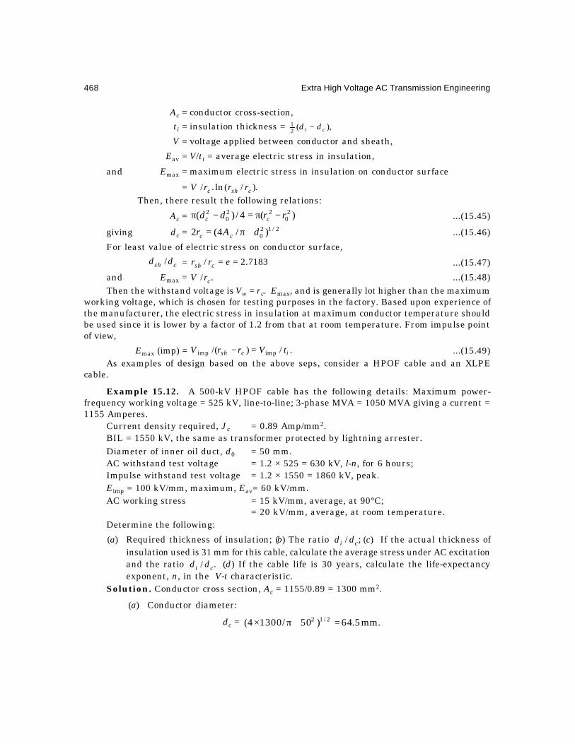
468 Extra High Voltage AC Transmission Engineering
Ac = conductor cross-section,
ti = insulation thickness = ),(21
ci dd −
V = voltage applied between conductor and sheath,
Eav = V/ti = average electric stress in insulation,
and Emax = maximum electric stress in insulation on conductor surface
= )./(ln./ cshc rrrVThen, there result the following relations:
Ac = )(4/)( 20
220
2 rrdd cc −π=−π ...(15.45)
giving dc =2/12
0 )/4(2 dAr cc +π= ...(15.46)
For least value of electric stress on conductor surface,
csh dd / = 7183.2/ == err csh ...(15.47)
and Emax = ./ crV ...(15.48)Then the withstand voltage is Vw = rc. Emax, and is generally lot higher than the maximum
working voltage, which is chosen for testing purposes in the factory. Based upon experience ofthe manufacturer, the electric stress in insulation at maximum conductor temperature shouldbe used since it is lower by a factor of 1.2 from that at room temperature. From impulse pointof view,
Emax (imp) = ./)/( impimp icsh tVrrV =− ...(15.49)As examples of design based on the above seps, consider a HPOF cable and an XLPE
cable.
Example 15.12. A 500-kV HPOF cable has the following details: Maximum power-frequency working voltage = 525 kV, line-to-line; 3-phase MVA = 1050 MVA giving a current =1155 Amperes.
Current density required, Jc = 0.89 Amp/mm2.BIL = 1550 kV, the same as transformer protected by lightning arrester.Diameter of inner oil duct, d0 = 50 mm.AC withstand test voltage = 1.2 × 525 = 630 kV, l-n, for 6 hours;Impulse withstand test voltage = 1.2 × 1550 = 1860 kV, peak.Eimp = 100 kV/mm, maximum, Eav= 60 kV/mm.AC working stress = 15 kV/mm, average, at 90°C;
= 20 kV/mm, average, at room temperature.Determine the following:
(a) Required thickness of insulation; (b) The ratio ;/ ci dd (c) If the actual thickness ofinsulation used is 31 mm for this cable, calculate the average stress under AC excitationand the ratio ./ ci dd (d) If the cable life is 30 years, calculate the life-expectancyexponent, n, in the V-t characteristic.
Solution. Conductor cross section, Ac = 1155/0.89 = 1300 mm2.
(a) Conductor diameter:
dc = mm.5.64)50/13004( 2/12 =+π×

Extra High Voltage Cable Transmission 469
Conductor thickness = mm.25.72/)( 0 =− ddc
If a ratio of )/( ci dd = e is assumed, then mm.2.1757183.2 == ci dd The correspondinginsulation thickness is
ti = mm.4.552/5.647183.12/)( =×=− ci dd
The maximum electric stress on the conductor surface is
Emax = kV/mm.53.19)5.645.0/(630/ =×=cw rV
and Eav = kV/mm.4.114.55/630 =
These are within the given values of 20 kV/mm and 15 kV/mm.
(b) Ratio )/( ci dd = 2.7183
(c) Since under impulse conditions the necessary thickness of insulation is 1860/60 = 31mm, the value given, the AC stresses are as follows:
Average stress during test = 630/31 = 20.3 kV/mm.
Average stress during operating life = )331/(525 × = 9.8 kV/mm, r.m.s.
ici tdd 2+= = mm.5.1263125.64 =×+∴ ci dd / = .25.64/5.126 ≈
(d) )2436530()3/525(6630 ×××=× nn
or (630/303.11)n = 30 × 365 × 4
giving .6.14)078.2log(
)436530log(=
××=n
Example 15.13. A 500 kV XLPE cable is required to be designed under the followingcontinuous working and testing conditions:
Maximum working voltage = 550 kV, r.m.s., line-to-line;Test voltages: Vac = 1100 kV, r.m.s., line-to-neutral;
Vimp = 2250 kV, peak, without lightning arresters;Average electric stresses:Eac = 30 kV/mm, Eimp = 65 kV/mm;Area of conductor, Ac = 2000 mm2. No central oil duct.
(a) Calculate di, the diameter to the outside of insulation, for least value of maximumstress and the magnitude of the stress on the conductor surface;
(b) If the actual value of ti is 35 mm based on impulse strength, calculate themaximum and average stresses in the insulation and compare with Eav(ac) of 30kV/mm;
(c) At a current density of 0.8 Amp/mm2, find the power tramsmitted at 550 kV.Solution.
(a) dc = mm.5.50)/20004()/4( 2/12/1 =π×=πcA
∴ di = mm.4.432/)5.503.137(andmm,3.1377183.2 =−== ic td
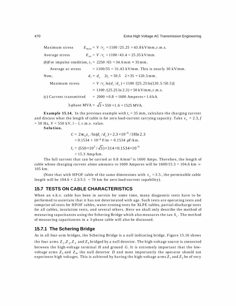
470 Extra High Voltage AC Transmission Engineering
Maximum stress Emax = .r.m.skV/mm,8.4325.25/1100/ ==crV
Average stress Eav = kV/mm.35.254.43/1100/ ==itV
(b)For impulse condition, ti = mm.35mm6.3465/2250 ≈=
∴ Average ac stress = 1100/35 = 31.43 kV/mm. This is nearly 30 kV/mm.
Now, di = mm.5.1203525.502 =×+=+ ic td
∴ Maximum stress = )]5.50/5.120ln(25.25/[1100)/ln(/ =cic ddrV
= r.m.s.kV/mm,50)3.2ln25.25/(1100 =
(c) Current transmitted = kA.6.1Amperes16008.02000 ==×
∴ 3-phase MVA = MVA.15256.15503 =××
Example 15.14. In the previous example with ti = 35 mm, calculate the charging currentand discuss what the length of cable is for zero load-current carrying capacity. Take rε = 2.3, f= 50 Hz, V = 550 kV, l – l, r.m.s. value.
Solution.
C = 3.2ln18/103.2)/ln(/2 90
−×=επε cir dd= 0.1534 × 10⁻⁹ F/m = 0.1534 µF/km.
Ic =63 101534.0314)3/10550( −××××
= 15.3 Amp/km.The full current that can be carried at 0.8 A/mm2 is 1600 Amps. Therefore, the length of
cable whose charging current alone amounts to 1600 Amperes will be 1600/15.3 = 104.6 km ≈105 km.
(Note that with HPOF cable of the same dimensions with 5.3=ε r , the permissible cablelength will be 104.6 × 2.3/3.5 = 70 km for zero load-current capability).
15.7 TESTS ON CABLE CHARACTERISTICSWhen an e.h.v. cable has been in service for some time, many diagnostic tests have to beperformed to ascertain that it has not deteriorated with age. Such tests are operating tests andcomprise oil tests for HPOF cables, water-treeing tests for XLPE cables, partial-discharge testsfor all cables, insulation tests, and several others. Here we shall only describe the method ofmeasuring capacitances using the Schering Bridge which also measures the tan iδ . The methodof measuring capacitances in a 3-phase cable will also be discussed.
15.7.1 The Schering BridgeAs in all four-arm bridges, the Schering Bridge is a null indicating bridge. Figure 15.16 shows
the four arms 321 ,, ZZZ and Z4 bridged by a null detector. The high-voltage source is connectedbetween the high-voltage terminal H and ground G. It is extremely important that the low-voltage arms Z3 and Z4, the null detector D and most importantly the operator should notexperience high voltages. This is achieved by having the high-voltage arms Z1 and Z2 be of very

Extra High Voltage Cable Transmission 471
Fig. 15.16 The high-voltage Schering Bridge.
high impedance as compared to the l.v. arms Z3 and Z4. Moreover, these are protected byparallel gas tubes which ground the points A and B in the event of a high voltage. It should beclear that the h.v. arms should never be permitted to breakdown so that their voltage ratingshould be very liberal as compared to the applied voltage.
The cable under test is used as arm Z1 which has its capacitance Cc in parallel with itsinsulation resistance Ri. These are denoted as C1 and R1, whose values are to be measured. Inthe commercial variety of the Schering Bridge, the capacitance and tan δ are calibrated directlyin arms Z3 and Z4. Arm Z2 is a lossless standard capacitor rated for the high voltage of thesupply. It is filled with Nitrogen or SF6 at very high pressure in order not to give partialdischarges. The source of a.c. supply, usually a high-voltage transformer, as well as all terminalsand leads should be free of discharges upto the voltage used in the test. As shown inFigure 15.16, the arm Z4 consists of a non-inductive resistor while arm Z3 is made up of acapacitor and resistor in parallel. Balancing is usually carried out, as in all a.c. bridges, in twostages, since two quantities have to be measured, namely C1 and R1 or tan δ . First, thereading of the null detector is brought to minimum value by adjusting C3 and then furtherminimized by changing R3. Most null detectors of today have built-in amplifier and are ofelectronic type so that very accurate balancing at extremely high sensitivities are possible.
The four impedances at frequency f and fπ=ω 2 are as follows:
Z1 = ;/1);1/(/1
122111
11
CjZCRjRCjR
ω=ω+=ω+
Z3 = )1/( 333 CRjR ω+ ; and Z4 = R4. Also, tan 11/1 CRω=δ .
When the bridge is balanced with zero current through the detector there results
4231 ZZZZ ⋅=⋅ Multiplying and collecting real and j-terms, there result the following relations:
231 CRRjω = .)](1[ 4231131312 RCRCRjCCRR +ω+ω− ...(15.50)
H
B
G
A
C1
Z1
R4
Z4C3
Z3
R3
Z2
C2
R1
V ω
D


Extra High Voltage Cable Transmission 473
At e.h.v. levels, there are very few 3-core designs but there are some designs where sucharrangement is preferred. In a single-core cable with metallic sheath there will exist someeddy-current loss which is eliminated in a 3-core cable. However, when three single-core cablesare laid together, by proper bonding of the metallic sheaths the sheath current is made nearlyzero. The following average values of sheath losses exist:
(a) 3 single-core cables: 132 kV–Total cable losses 100 watts/m broken down into conductorlosses 82 w, dielectric losses 7 w, and sheath eddy-current losses 11 w, per metrelength.
(b) Pipe-type cable–3-core cable. Loss in pipe amounts to nearly 20 to 30 watts/metre in765 kV system; 10% lower for 345 kV system.
In symmetrically manufactured 3-phase cables, such losses are normally not present.However, in every type of cable, the sheath must be made with a definite cross-section in orderto carry the short-circuit current in the event of a phase-to-ground fault. The design of metallicsheath and pipe is not considered here.
Referring to Figure 15.17, the 3-core cable represents an equivalent capacitive networkas shown in Figure 15.18 (a), where Cc = capacitance between any two cores, and Cg = capacitancebetween any conductor and sheath. It will be assumed that these are balanced so that all threeCc's are equal and all three Cg's are also equal. In order to measure Cc and Cg individually, twotests are given. In the first test, shown in Figure 15.18(b), two of the cores are connectedtogether and are both connected to the sheath. If the measured capacitance on a ScheringBridge is C1, then obviously,
C1 = 2Cc + Cg. ...(15.55)Next, as shown in Figure 15.18(c), all three cores are connected together and the
capacitance between these and the sheath is measured as C2. ThenC2 = 3Cg. ...(15.56)
From equations (15.55) and (15.56), the values of Cc and Cg are
Cg = C2/3, and Cc = 6/2/ 21 CC − . ...(15.57)
In this treatment, dielectric losses have been neglected.
Fig. 15.18 Capacitance network of 3-phase cable.
15.8 SURGE PERFORMANCE OF CABLE SYSTEMSE.H.V. cables nearly always have one end connected to an e.h.v. over-head line and the otherto the e.h.v. bushing and winding of a transformer of very large capacity. A lightning surge
Cg Cg
Cg
Cc Cc
Cc
( )a
Cg
Cc Cc
( )b
C C + C1 = 2 c g
Cg
Cg Cg
( )c
C C2 = 3 g

474 Extra High Voltage AC Transmission Engineering
originating in the overhead line is brought through the cable and strikes the transformer. Dueto the low surge impedance offered by the cable its voltage becomes low initially but by repeatedreflections, the voltage has a chance of building up to high values. Thus, each systemconfiguration has to be analyzed on a case by case basis in order that proper class of lightningarresters can be installed if necessary. Usually these arresters are provided for transformerprotection so that the BIL of the cable is made the same as that of the transformer. In thissection, an analysis of a typical case will be presented of the travelling wave voltages in a cable-connected system between an overhead line and a transformer. It will be assumed that thewinding shows a travelling wave pattern for the surge in presenting a surge impedance to avoltage wave. Details of voltage propagation properties in a winding cannot be dealt with heresince at the first incidence of the surge it behaves as a pure capacitive network so that thesurge reaches the far end (usually grounded) practically instantaneously. After the capacitivenetwork is fully charged, current commences to flow in the inductance of the winding so thatthe concept of surge impedance can be used. For the sake of illustrating the build up of voltagewe will use a surge-impedance model of the transformer and its value will be taken as 1000ohms.
Consider the three-component system of Figure 15.19, consisting of an overhead line ofsurge impedance Z0 connected to a cable of length L with a surge impedance Zc = 1/νC and adielectric with relative permittivity rε .
Fig. 15.19 Overhead line connected to transformer h.v. winding through e.h.v.cable for illustrating surge performance.
Thus, the velocity of propagation of surge in the cable is v = light velocity/ rε , with the
transit time vLtc /= . For instance, considering an XLPE cable with rε = 2.25, the velocity is
(2/3) × light velocity = 2 × 10⁵ km/sec. The time delay for 1 km length is 5 µs. The last componentis the transformer e.h.v. winding with a surge impedance Zt offering a travel time tt for thesurge from the bushing to the grounded end. A lightning surge of peak value Vw is assumed totravel on the line when it strikes the junction Jcl of the cable and line. For the sake of analysisthe step response will be discussed, and the line so long that reflections arriving from its farend will be neglected. Also, all attenuations will be neglected.
Referring to Figure 15.19, the reflection and refraction (transmission) factors are as follows:At junction Jcl :(a) For a wave coming from line:
Reflection coefficient, Kr = 0
0
ZZZZ
c
c
+−
Refraction coefficient, Kt = 0
2ZZ
Z
c
c
+
Line Trans.Cable
ZoZc, εr, V, tc, Zt, tt
Jcl Jct G

Extra High Voltage Cable Transmission 475
(b) For a wave coming from transformer:
Kr = c
tc
c
ZZZ
KZZZZ
+=
+−
0
0
0
0 2,
At junction Jct (between cable and transformer):(c) For a wave coming from cable:
Kr = 0
2,
ZZZ
KZZZZ
t
tt
ct
ct
+=
+−
(d) For a wave coming from transformer:
Kr = tc
ct
tc
tc
ZZZ
KZZZZ
+=
+− 2
,
At the grounded end of the transformer : Kr = – 1; Kt = 0.A few examples will make the Bewley Lattice Diagram clear for the build-up of voltage at
the two ends of the cable and the transformer terminal.
Example 15.16. A 500 kV overhead line with surge impedance Z0 = 275 ohms is connectedto an XLPE cable with v = 2 × 10⁵ km/sec and 1 km in length. From Table 15.2, its surgeimpedance is 36 ohms. The far end of the cable connects a transformer with Zt = 1000 ohmswhose other end is solidly grounded. The transit time of surge through the winding is also 5 µs,the same as for the cable. See Figure 15.20. A step voltage of 1 per unit is travelling on the line.
Fig. 15.20 Details of system for Example 15.16
(a) Calculate the ten reflection and refraction coefficients;(b) Draw the Bewley Lattice Diagram for the travel of surge in the cable and transformer
upto 50 µs;(c) On a volt-time diagram, sketch the voltages at the two ends of the cable upto 50 µs.
Solution.(a) At junction Jcl:For a wave coming from line:
Kr = (36 – 275)/(36 + 275) = – 0.7685∴ Kt = 1 + Kr = 0.2315 (= 72/311)For a wave coming from transformer end or junction Jct :
Kr = (275 – 36)/(275 + 36) = + 0.7685, and Kt = 1.7685.At junction Jct:For a wave coming from cable into transformer:
Kr = (1000 – 36)/(1000 + 36) = + 0.9305, and Kt = 1.9305For a wave coming from transformer into cable:
Kr = (36 – 1000)/(36 + 1000) = – 0.9305, and Kt = 0.0695.
275 ohms
Vw = 2400 kVStep
Vc
Zc
Cable Vt = 1725 kV
1100 ohms5 km
Trans.

476 Extra High Voltage AC Transmission Engineering
At ground end: Kr = – 1, and Kt = 0.These 10 coefficients are shown on Figure 15.21.(b) The Bewley Lattice Diagram can now be drawn. All salient values are shown on
Figure 15.21, and are explained below:
Fig. 15.21 Bewley Lattice Diagram for performance of surge in Example 15.16.
Since the travel time through both cable and transformer are equal to 5 µs, three verticallines are drawn with distances of separation equal. 5 µs intervals are marked vertically to somescale. The following sequence of events takes place: The incident surge of + 1 per unit entersthe cable from the line and has the value 0.2315 in the cable. This strikes the transformer after5 µs. The transmitted voltage into the winding is 1.9305 × 0.2315 = 0.447, while the reflected
Jcl Jct5 sµ 5 sµ1
1
– 11
1
11.7685
– .7685.2315
.9305
.0695– .9305
1.9305
0
G
.2315
+1
.6125
.885
.951
.893
.746
0,
10,
20,
30,
40,
50,
.447
.736
.868
.863
.755
.2315
.1655
.0946
.0248
– .025
– 0.64
– .083 – .023
– .863
– .033.027
– .868
.037.088
– .736
.123.154
– .447
.2154
– .06
– .060
– .051
– .031
.803
– .048
.055
.1826
.32
.808
.685
.416
.447
– .755
.755
.863
.868
.736
0
0
0
0
0
.7685

Extra High Voltage Cable Transmission 477
wave into the cable is 0.9305 × 0.2315 = 0.2154, still positive. The latter wave travels back tothe junction Jcl to the line where the reflected value is 0.2154 × 0.7685 = 0.1655. The furtherprogress of this voltage wave is indicated on the figure. In the meanwhile, the first wave ofamplitude 0.447 entering the transformer from the cable hits the grounded end and reflectstotally negative with – 0.447 p.u. This voltage strikes the cable at Junction Jct and reflects witha value (– 0.447 × 0.9305) = – 0.416 which travels back to the grounded end. The voltageentering the cable is (– 0.447 × 0.0695) = – 0.031 which now travels to junction Jcl of cable andline, and reflects with the value (– 0.031 × 0.7685) = – 0.0238.
At this instant, namely at 20 µs from the start, the total voltage of junction Jcl is (0.2315+ 0.2154 + 0.1655 + 0.123 + 0.0946) = 0.885. At 10 µs, its value was (0.2315 + 0.2154 + 0.1655) =0.6125. (Also, 0.885 = 0.6125 + 0.123 + 0.0946). Voltages at the transformer terminal are asfollows: At 5 µs, 0.447; At 15 µs, 0.447 – 0.447 + 0.3196 – 0.416 = – 0.0964.
A summary of voltages is given below:
Line–Cable Junction, Jctµs Cable–Transformer Junction,Per Unit Voltage Jctµs Per Unit Voltage
0 0.2315 5 0.44710 0.2315 + 0.2154 + 0.1655 = 0.6125 15 0.447 – 0.031 + 0.32 = 0.73620 0.6125 + 0.123 + 0.0946 = 0.885 25 0.736 – 0.051 + 0.183 = 0.86830 0.885 + 0.037 + 0.0284 = 0.951 35 0.868 – 0.06 + 0.055 = 0.863
(1.7585 × 0.037)40 0.951 + 1.785 × (– 0.033) = 0.893 45 0.863 – 0.06 – 0.048 = 0.75550 0.893 – 1.785 × 0.083 = 0.746
(c) The Volt-Time diagrams for the two junctions are shown in Figure 15.22.
Fig. 15.22 Volt-Time diagram for voltages at line—cable (Jcl) and cable—transformer(Jct) junctions in Example 15.16.
Example 15.17. Repeat Example 15.16 if the travel time in the transformer winding is10 µs instead of 5 µs.
Solution. As shown in Figure 15.23, the spacing between the three vertical lines areproportional to 5 and 10 µs. The progress of the voltage waves is given and the final voltages
00 10 20 30 40 50 60
1.0
0.5
.2315
.447
.6125
.736.868
.755
.746
.893.951
.885
P.u. voltage
Jcl
Jct
Voltages
µs

478 Extra High Voltage AC Transmission Engineering
are summarized below:t, µs Voltage at Jcl, P. U. t, µs Voltage at Jct, P.U.
0 0.2315 5 0.44710 0.2315 + 1.7685 × 0.2154 = 0.6125 15 0.447 + 0.32 = 0.76720 0.6125 + 1.7685 × 0.154 = 0.885 25 0.767 – 0.031 + 0.229 = 0.96730 0.885 + 1.7685 × 0.079 = 1.025 35 0.967 – 0.0222 + 0.1172 = 1.0640 1.025 – 1.7685 × 0.02 = 1.0853 45 1.06 – 0.045 + 0.051 = 1.06650 1.0853 – 1.7685 × 0.02 = 1.05 55 1.066 – 0.029 – 0.03 = 1.00660 1.05 – 1.7685 × 0.0436 = 0.972
The Volt-Time diagrams are shown in Figure 15.23.
Fig. 15.23 Bewley Lattice Diagram and Volt-Time diagram for Example 15.17.
15.9 GAS INSULATED E.H.V. LINES
15.9.1 GeneralE.H.V. lines insulated with SF6 gas are being used extensively all over the world for voltagesupto 1200 kV and for lengths upto 5 km. The longer lengths exist in oil fields. Gas insulatedlines (GIL) also known as Bus Ducts, are not flexible but they can be installed in tunnels orabove ground, in horizontal, vertical or inclined positions. Typical dimensions of inner cylindricalconductor and outer coaxial cylindrical enclosure are given in Table 15.4 as well as gas pressure,maximum electric stress on the conductor surface for single-phase lines, and the capacitanceand surge impedance values. They carry currents in the range 2,000 to 10,000 Amperes.
P.u. voltage
1.0
0.5
00 10 20 30 40 50 60
.2315
.447.6125
.787.885
.9651.0251.06 1.085 1.05
1.006.972
Voltages
µs
JclJct
.2315
.6125
.885
1.025
1.085
1.05
1.006.972
0,
10,
20,
30,
40,
50,
60,
.447
.767
.965
1.06
1.066
Jcl Jct
5 sµ 10 sµ
.447
.2315
.1655 .32
.1184 .645
.06.415
026 .651
– .016 .356
– .034
.2154
– .447
.154
– 0.32
.079
– .645
.034
– .415
– .02
– .651
– .356
–.044
G

Extra High Voltage Cable Transmission 479
Table 15.4 Typical Properties of E.H.V. GIL's
Voltage Rated, kV 220 275 345 500 750Maximum, kV 245 300 362 525 765 (Also 800)Conductor Diameter, cm 10 15 12 25 15 (25)Enclosure Diameter, cm 40 40 50 60 70 (70)Insulation Clearance, cm 15 12.5 19 17.5 27.5 (22.5)ln (Re/rc) 1.386 0.981 1.435 0.875 1.54 (1.03)
Emax = cmkVrRr
V
cec/,
)/ln(.3/max
10.2 11.8 12.14 13.86 19.1 (17.9)
Capacitance, nF/km 40 56.6 38.7 63.5 36 (53.9)C = 55.55/ln (Re/rc)Surge Impedance, Z0 83.3 59 86 52.5 92.6 (62)Gas Pressure, Atm. 2–4 2–4 3–4 3–4 3–4
Thus, the GIL has a capacitance of roughly five times that of an over-head line but 30% ofthat of a cable with solid insulation. Its surge impedance is nearly double that of cables. In aGIL, the inner tubular conductor is supported by epoxy resin spacers which may be of the post,disc, or cone types. These are shown in Figure 15.1 (j) and (k). The electric stress on thesespacers is kept below 30 kV/cm (3 kV/mm). The inner conductor and outer enclosure are madefrom Aluminium alloy. While these are mostly stiff, some designs for extremely high voltages(1200 kV) use flexible inner conductor. The maximum allowable temperature of the insulatorsis 90°C while the gas temperature is much lower.
15.9.2 Properties of SF6 GasTechnical literature on properties and uses of SF6 gas as an insultant in cables, switchgear andother electrical equipment is so extensive and voluminous that only a few salient points needbe given here for completeness. SF6 is five times heavier than air with a specific gravity (density)of about 6 grams/litre. It liquifies at – 40°C at 3.6 atmospheres pressure, and at – 10°C at about10 atmospheres. The pressure used in GIL's is between 2 to 4 atmospheres (1 kg/cm2 = 14.2Lbs/in2 = 0.966 Atm ≈ 1 Atm.). Thus, the gaseous phase exists at temperatures in excess of– 35°C at these pressures, and at ordinary temperatures SF6 is a gas. It is colourless, odourless,non-toxic, non-combustible, chemically extremely stable, and inert upto 500°C. SF6 is calledelectronegative as it captures free electrons to form heavy negative ions which are relativelyimmobile in the usual applied electric fields in GIL's which gives the gas a very stable insulatingproperty even in the event of small discharges. This property of capture of free electrons isextremely important in arcing chambers of circuit breakers, and during phase-to-ground (or,conductor-to-enclosure) faults in GIL's. The dielectric strength of SF6 is 2 to 3 times that of airat the same pressure. Table 15.5 gives the comparison between the electric strengths of air,insulating oil, and SF6 gas.
Table 15.5 Typical Dielectric Strengths of Air, Oil, and SF6
Pressure, Atm. 1 2 3 4 5 6
Air, kV/mm 1 1.3 1.6 1.9 2.2 2.5 (Linear)Oil, kV/mm 3 3 3 3 3 3 (Constant)SF6, kV/mm 2 2.9 3.68 4.5 5 5.4 (Nonlinear)
480 Extra High Voltage AC Transmission Engineering
Since the pressure used in GIL's is quite low but above atmospheric, seals are easy tomake and the leakage of gas, if any, is from the inside of the GIL into the external air.
For extremely large currents of the order of 10 kA, liquid cooling of the external housingis used by laying pipes alongside the housing. In some installations the SF6 gas is circulatedand cooled. Because of transportation limitations, bus ducts (GIL's) are made in short lengthsand there are numerous joints either of the welded or the bolted type or plug-in joints in a longlength, for both the internal conductor and the external housing or enclosure.
Review Questions and Problems
1. (a) Upto what e.h.v. levels are cables manufactured to date? List the voltage levelsused.
(b) Name the four classifications of cables according to the insulations used.(c) Give briefly the properties of these four dielectrics giving examples.(d) Expand the following abbreviations: O-F, HPOF, KP, MPa, XLPE, EPR, PP,
PMP, PPLP, PMPLP, GIL.(e) What are the possible causes of initiation of water trees in XLPE insulation?
What are the harmful effects of these? How are they suppressed or minimized?(f) What are the average values of εr, tan δ, and withstand kV/mm of the following?
(1) un-impregnated Kraft paper, (2) impregnated Kraft paper in cables, (3) PPLP,(4) XLPE, (5) SF6.
2. A GIL for 500 kV has a conductor diameter of 20 cm and enclosure diameter of 60 cm.Calculate the following:
(a) Insulation clearance;(b) Average electric stress at 525 kV, line-to-line;(c) Maximum electric stress at 525 kV, l-l;(d) Capacitance per 100 metres;(e) Charging MVAR for 1 km at 525 kV, l-l;(f) If the breakdown stress of SF6 at the pressure used is 4.5 kV/mm, what is the
factor of safety used?3. In a Schering Bridge experiment, a 10-metre specimen of 400-kV O-F cable with a
designed value of capacitance of 0.3 nF/m and tan δ = 0.2% is tested at full ratedvoltage of 400 kV, l-l (230 kV l-n). The values of components at 50 Hz in Figure 15.16are as follows at balance : C2 = 1 nF, R4 = 1 K, R3 = 3 K, and C3 = 2 nF. Calculate(a) the capacitance of the cable sample per metre,(b) tan ,δ(c) insulation resistance per metre, and(d) the voltage across the l.v. arm of bridge at 230 kV.
Derive the equations which you have used.
Extra High Voltage Cable Transmission 481
4. Describe the tests required to measure Cc and Cg of a 3-phase unbelted cable whereCc = inter-core capacitance and Cg = core-to-sheath capacitance. If the two measuredvalues are 1.2 µF and 0.9 µF, calculate Cc and Cg. (There are two sets of values).
5. (a) A sample of XLPE when tested at 50 Hz gave breakdown stresses of 40 kV/mmat 1 hour and 50 kV/mm at 6 minutes. Assuming En.t = constant, calculate thevalue of exponent n.
(b) Discuss the significance of this property in designing the insulation of a cablethat is to work satisfactorily for many years.
(c) If the test is given for 15 minutes what value of stress will cause breakdowninitially?
6. (a) In the worked examples 15.3, 15.4, and 15.5, check the values of exponent b andscale factor E0 by utilizing a different set of values for P and E out of the givendata.
(b) Derive all equations used in solving the design problems.(c) Discuss the significance of the breakdown-probability distribution of the Weibull
type on cable designs.7. In a large power station for which a 275-kV XLPE is required to be installed, the
following design specifications are used: Lifetime-30 years; AC test withstand duration-3 hours; V0 = maximum operating voltage = 1.05 × rated voltage. BIL = 1050 kV.Temperature deterioration coefficients: K1 (ac) = 1.1; K1 (imp) = 1.25. Maximumoperating temperature of conductor = 80°C. K2 (ac) = 3.54. K2 (imp) = 1.1. Safetyfactors K3 = 1.1 for both types of voltage. Calculate the following:
(a) Life exponent n;(b) Voltage to be used in impulse and ac tests;(c) If the ac test is conducted at the elevated temperature of 80°C, what would be
the value of test voltage used during the 3-hour test?8. A 400-kV overhead line with Z0 = 312 ohms is connected to a grounded-neutral
transformer winding with Zt = 1250 ohms and having a travel time of 7.5 µs for thesurge, through a 400 kV cable. The cable has the following details: conductor diameter
= 50 mm, sheath diameter = 100 mm, permittivity rε = 3.6. A surge of 1000 kV peak
is travelling on the line when it hits the junction of cable and line. Calculate or drawthe following:
(a) Surge impedance of cable;(b) Travel time of surge through cable if its length is 395 metres;(c) Draw the Bewley Lattice diagram upto 30 µs;(d) Draw the volt-time diagrams for voltages at the two ends of the cable and give
the maximum attained within the 30 µs duration;(e) If the transformer had been connected directly to the overhead line, what would
have been the voltage at the high-voltage terminal of the transformer?( f ) If the BIL of the transformer is 1425 kV and the protective ratio of lightning
arrester is 1.4, will the arrester discharge with the cable in and without thecable?

Books1. Alston, L.L.: High Voltage Technology. Oxford University Press, 1968. (Harwell Post-
Graduate Series).
2. Aseltine, J.A.: Transform Methods in Linear System Analysis . Mc-Graw-Hill, 1980.
3. Bewley, L.V.: Travelling Waves in Transmission Systems. John Wiley, (1933, 1951),Dover, 1963.
4. Bewley, L.V.: Two-Dimensional Fields in Electrical Engineering. (McMillan), Dover,1963.
5. Bowdler, G.W.: Measurements in High Voltage Test Circuits. Oxford, Pergamon Press,1973.
6. Considine, D.M.: Handbook of Energy Technology. McGraw-Hill Book Co., 1977.
7. Craggs, J.D., and Meek, J.M.: High Voltage Laboratory Technique. ButterworthScientific Publications. 1954.
8. Craggs, J.D., and Meek, J.M.: Electrical Breakdown of Gases. Oxford Clarendon Press.1953.
9. Craggs, J.D., and Meek, J.M.: Electrical Breakdown of Gases. (Ed.). Chichester, JohnWiley, 1978.
10. Edison Electric Institute : E.H.V. Transmission Reference Book. (General ElectricCo.), 1968.
11. Electrical Power Research Institute. (Palo Alto, Calif.): Transmission Line ReferenceBook Above 345 kV. 1975.
12. Greenwood, A.: Electrical Transients in Power Systems. Wiley-Interscience, 1971.13. Hayashi, Shigenori : Surges on Transmission Systems. Denki-Shoin, Kyoto, Japan.
1955.
14. Kind, Dieter : An Introduction to High-Voltage Experimental Technique. (Translatedby Y.Narayana Rao). Wiley Eastern, 1979.
15. Kuffel, E. and Abdullah, M.: High Voltage Engineering. Oxford Pergamon Press. 1970.
Bibliography
Bibliography 483
16. Kuffel, E. and Zaengel, W.S.: High Voltage Engineering Fundamentals. OxfordPergamon Press. 1984.
17. Lee, T.H.: Physics and Engineering of High Power Switching Devices. M.I.T. Press,Cambridge, Mass. 1975.
18. Lewis, W.W.: Protection of Transmission Systems Against Lightning. John Wileyand Sons, 1950.
19. Loeb, L.B.: Basic Processes of Gaseous Electronics. University of California Press,Berkeley, 1960.
20. Loeb, L.B.: Electrical Coronas, U. of Calif. Press, 1965.
21. V.N. Maller and M.S. Naidu : Advances in High Voltage Insulation and Arc Interruptionin SF6 and Vacuum. Pergamon Press, 1981.
22. McAllister, D. (Ed.) : Electric Cables Handbook. Granada Publishing Co., London. (8Grafton St., W1X 3LA), 1987.
23. Naidu, M.S. and Kamaraju, V.: High Voltage Engineering. Tata-McGraw-Hill PublishingCo., 1982.
24. Radzevig, D.K.: High Voltage Engineering. (Translated from Russian by M. Chaurasia).Khanna Publishers, New Delhi.
25. Ragaller, K. (Ed.): Surges in High-Voltage Networks. Plenum Press, New York andLondon, 1979.
26. Ragaller, K. (Ed. Brown Boveria Co.): Current Interruption in High-Voltage Networks.Plenum Press, 1977.
27. Rudenberg, R.: Transient Performance of Electric Power Systems. McGraw-Hill BookCo., 1950.
28. Rudenberg, R.: Electric Shock Waves in Power Systems. Harvard University Press,Cambridge, Mass. 1968.
29. Scott, E.J. : Transform Calculus. Harper and Row, New York. 1955.
30. Stevenson, W.D., Jr.: Elements of Power System Analysis . 2nd and 4th Editions.McGraw-Hill International Book Co., 1982.
31. T. Tanaka and A. Greenwood: Advanced Power Cable Technology.
Vol. 1: Basic Concepts and Testing, 1983.Vol. 2: Present and Future, 1983. C.R.C. Press, Florida.
32. Westinghouse Trans and Distribution Ref Book. IBH—Oxford. 1950.
33. Zahn, M: Electromagnetic Field Theory—A Problem-Solving Approach. John Wileyand Sons. 1979.
34. T.J. Gallagher and A.T. Piermain : High Voltage Measurement: Testing and Design.Chichester, Wiley. 1983.
35. N. Hylten-Cavallius: High Voltage Laboratory Planning. H.V. Test Systems (EmileHaefely).
36. EPRI: Wind-Induced Conductor Motion, 1979.
484 Extra High Voltage AC Transmission Engineering
Begamudre, Rakosh Das1 Successive refraction of travelling waves on multi-conductor transmission lines.
Journal, Institution of Engineers (India), April 1957.
2. Investigation of corona loss and RI from h.v. overhead dc transmission lines. WithR.M. Morris. Trans. IEEE, PAS, Jan., 1964, pp. 10–17.
3. Corona pulses and RI under h.v. dc. ibid, May 1964, pp. 483–491.
4. Radio noise levels of dc transmission lines. Bull. of the Radio and EE Div., NationalRes. Council of Canada, Ottawa. Sept. 1964.
5. Corona pulses and RN levels from a water drop under several types of excitation.Letter to Editor, Proceedings IEEE, 1967, p. 2164.
6. RI levels of transmission lines and corona pulse characteristics. Trans. CanadianEng. Inst., Oct., 1970, pp. 1–7.
7. The absolute method of pre-determination of RN levels of e.h.v. ac and dc Transmissionlines. Symposium on Selection of Next EHV Transmission Voltage for India. CentralBoard of Irrigation and Power, New Delhi. Publication No. 142, May 1980.
8. Voltage gradient calculation of 345 kV to 1500 kV transmission line conductors. ibid.
9. Next higher transmission voltage for India. C.B.I.P. Publication No. 162, Dec. 1980.10. Switching surge testing of transformers. Indian Transformer Manufacturers'
Association. Symposium, Dec. 1980.
11. Design of coils for representing long lines on a TNA. Part I : Theoretical considerations.Part II: Practical considerations. C.B.I.P. 49th Research Meeting Proceedings. Sept.1981.
12. Effect of line-coil representation in a TNA on switching transients of transmissionlines. (With S. Subhash, K.S. Meera, and M.Kanya Kumari). C.B.I.P. Publication No.170, 51st Research Meeting, Vadodara, 1984.
13. Impulse generators for lightning and switching surges. Design and performance.Technical Report No. 106, Central Power Research Institute, Box 1242, Bangalore—560 012.
14. Design of cages for corona studies. Technical Report No. 109, C.P.R.I., Bangalore.
15. Limits for interference fields from e.h.v. and u.h.v. power transmission lines: RI,AN, and E.S. fields. C.B.I.P. Publication No. 170, 1984. (Malcha Marg, Chanakyapuri,New Delhi, 110021.)
16. Formulas for calculation of excitation function of corona from RN fields of long e.h.v.lines. Conference on E.H.V. Technology. IEEE-IISc-IE (Ind.), Bangalore. Aug. 1984.
17. E.S. field, AN, and RI of 400 kV to 1300 kV lines, existing and proposed for India, andcomparison of AN levels of single-phase and three-phase test lines. (With R. Aroraand J. Senthil). ibid. (Volume of Conference Papers).
18. Effect of conductor size on e.h.v. transmission-line problems for 750 kV, 1000 kV and1150 kV. (With S. Ganga). Proceedings, 2nd National Power Systems PlanningConference, Jawaharlal Nehru Technical University, Saifabad, Hyderabad, India. Sept.1983.

Bibliography 485
19. Procedures for e.h.v. line-insulation designs based upon transient overvoltages.C.B.I.P. Publication No. 177. 52nd Research Meeting, Aurangabad. 1985.
20. Procedures for e.h.v. line designs based upon steady-state operating limits. ibid.21. A method of solving surge phenomena on e.h.v. lines including attenuation caused by
corona loss and resistance. ibid.
22. Energy and electrical power equipment development. State of the art speech. 1stNational Power Systems Planning Conference, Annamalai University, India. Sept.1982.
23. Energy development and human progress. Keynote address, Institution of Engineers(India), Kanpur Branch. 15 Sept. 1983.
24. Surge transfer in multi-winding transformers: Failures and remedies. (With P.Sivakumar). Electrical India, 31 Dec. 1984.
25. Investigation of overvoltage conditions in multi-winding transformers by calculationand model studies. (With P. Shivakumar). Proc. of 52nd R. & D. Session, C.B.I.P.Publication No. 177, Aurangabad. February 1985.
Monographs and Catalogues1. ALCOA: Conductor Motion Control. Feb. 1976. (Massena, N.Y.).
2. Electrical Manufacturing Co. Calcutta, Catalogue on Line Material and Hardware.
3. High Voltage Test Systems—ASEA, Haefely, Micafil. High Voltage LaboratoryEquipment.
4. I.E.E. Monograph Series 18: Computation of Power System Transients. J.P. Bickford(Ed.), Peter Peregrinus Press, London, U.K., 1976.
5. I.E.E.E. Brown Book: Industrial and Commercial Power System Analysis . IEEEStandard—399; 1980.
6. International Symposium on Controlled Reactive Compensation. IREQ—EPRI. 1979.
7. Morched, A.S.: Transmission Line Energization Transients. Division of High VoltageSystems. The University of Trondheim, Norway. 1972.
8. Siemens Power Engineering: Special Issue on High Voltage Technology, Vol. III,1981.
9. UPSEB Statistics at a glance. Planning Wing, Uttar Pradesh State Electricity Board,Shakthi Bhavan, Ashok Marg, Lucknow, U.P., India. 1984.
Brown Boveri Review1. J. Glavitsch: Power Frequency Overvoltages in Ehv Systems. 1964, pp. 21–32.
2. W. Frey: Considerations Governing Choice of Voltage Level for Longdistance High-capacity Transmission Systems. ibid, pp. 5–9.
3. P. Althammer and R. Petitpierre: Switching Operations and Switching Surges inSystems Employing EHV. ibid, pp. 33–46.
4. A. Goldstein: Coordination of Insulation and Choice of Lightning Arresters. ibid, pp.47–55.
486 Extra High Voltage AC Transmission Engineering
5. E. Ruoss and P. Djurdjevic: Network Analyzer for Studying Transient Phenomena inH.V. Networks. 1968, pp. 734–739.
6. A. Braun, A. Eidinger, and E. Ruoss: Interruption of Short-Circuit Currents in H.V.AC Networks. 1979. pp. 240–254.
7. J. Kopainsky and E. Ruoss: Interruption of Low Inductive and Capacitive Currents InH.V. Systems. ibid, pp. 255–261.
8. E. Ruoss: Overvoltages on Energizing H.V. Lines. 1979, pp. 262–270.
9. U. Burger: Insulation Coordination and Selection of Surge Arrester. 1979, pp. 271–280.
10. A. Eidinger and R. Schaumann: Sulphur Hexafluoride SF6. 1979, pp. 303–307.
Emile Haefely Publications1. K. Feser: Transient Behaviour of Damped Capacitive Dividers of Some M.V. IEEE
Transactions, PAS–93, 1974, pp. 116–121. (Reprint by E. Haefely et cie).
2. K. Feser: A new type of voltage divider for the measurement of high impulse and acvoltages. (Translated from Bulletin ASE, Nr. 19, pp. 929–935).
3. K. Feser: Problems Related to Switching Impulse Generation of H.V. Test Plants.Bulletin ASE, (SAE), vol. 65, 1974, pp. 496–508.
4. A. Rodewald: Transient Phenomena in the Marx Multiplying Circuit after Firing theFirst Coupling Spark Gap. Bulletin ASE, vol. 60, 1969, pp. 37–44.
5. K. Feser: Influence of Corona Discharges in the Breakdown Voltage of Airgaps. Proc.IEE, vol. 118, No. 9, Sept. 1971, pp. 1309–1313.
6. K. Feser: Mechanism to Explain the Switching Impulse Phenomena. Schweiz Tech.Zeit. 1971, pp. 937–946.
7. P. Mathiessen: La Production de hautes tensions d'essais. 'Le Monteur-Electricien',No. 4, 1972, pp. 11–22.
8. W. Muller, A. Rodewald, and H. Steinbigler: Stro β Strom Labor.
9. G. Reinhold: U.H.V. dc Power Supplies for Large Currents.
10. Th. Praehauser: Measurement of Partial Discharges in H.V. Apparatus With BalancedCircuit. Bulletin ASE, 1973, pp. 1183–1189.
11. Th. Praehauser: Locating Partial Discharges in H.V. Equipment. Bulletin ASE(Association of Swiss Electrical Engineers), 1972, pp. 893–905.
I.E.E.E. Transactions—Power Apparatus and Systems1. G.E. Adams: Voltage Gradients on H.V . Transmission Lines. 1955, pp. 5–11. (A.I.E.E.
Transactions).2. A.S. Timascheff: Fast Calculation of Gradients of a 3-phase Bundleconductor Line
with Any Number of Sub-conductors. 1971, pp. 157–164, Also, 1975, pp. 104–107, and1961 (AIEE Trans.), pp. 590–597.

Bibliography 487
3. S.P. Maruvada and W. Janischewskyj: Electrostatic Field Calculation of ParallelCylindrical Conductors. 1969, pp. 1069–1079.
4. M.S. Abou-saeda and E. Nasser: Digital Computer Calculation of Potential and ItsGradient of a Twin Cylindrical Conductor. 1969, pp. 1802–1814.
5. C.H. Gary: Corona Inception Field Calculation. Generalization of Peek's Law. 1972,pp. 2262–2263.
6. R.M. Morris and P.S. Maruvada: Conductor Surface Voltage Gradients on BipolarH.V. DC Transmission Lines. 1976, pp. 1934–1945.
7. IEEE Corona and RN Working Group: A Survey of Methods for Calculating VoltageGradients. 1979, pp. 1996–2014.
8. IEEE RN Subcommittee—AN Task Force. A Guide for the Measurement of AudibleNoise from Transmission Lines. 1972, pp. 853–856.
9. D.E. Perry: An Analysis of AN Levels Based Upon Field and 3–Phase Test LineMeasurements. 1972, pp. 857–865.
10. H. Kirkham and W.J. Gajda, Jr.: A Mathematical Model of Transmission Line AN,1983, pp. 710–728.
11. V.L. Chartier and R.D. Stearns: Formulas for Predicting AN from Overhead H.V. ACand DC Lines. 1981, pp. 123–128.
12. IEEE Task Force on Corona: A Comparison of Methods for Calculating Audible Noisefrom H.V. Transmission Lines, 1982, pp. 4090–4099.
13. N. Kolcio, J. Diplacido, and F.M. Dietrich: Apple Grove 750 kV Project—2-year StatisticalAnalysis of AN. 1977, pp. 560–570.
14. G.W. Juette and L.E. Zaffanella: RN, AN, and Corona Loss of E.H.V. and U.H.V.Lines Under Rain: Predetermination based on cage tests. 1970, pp. 1168–1178.
15. G.W. Juette and L.E. Zaffanella: RN Currents and AN on Short Sections of U.H.V.Bundled Conductors. 1970, pp. 902–913.
16. C.H. Gary: The Theory of the Excitation Function. 1972, pp. 305–310.
17. M.R. Moreau and C.H. Gary: Pre-determination of RI Level of H.V. TransmissionLines. I—Pre-determination of the Excitation Function. II–Field Calculating Methods.1972, pp. 284-304.
18. IEEE RN Subcommittee: A Field Comparison of RI and TVI Instrumentation. 1977,pp. 863–875.
19. N. Giao Trinh and P. Sarma Maruvada: A Method of Predicting The CoronaPerformance of Conductor Bundles Based Upon Cage Test Results. 1977, pp. 312–325.
20. W.C. Guyker, J.E. O'Neil, and A.R. Hileman: Right of Way and Conductor Selectionfor the Alleghany Power System, 500-kV Transmission System. 1966, pp. 624–632.
21. P. Sarma Maruvada and N. Giao Trinh: A Basis for Setting Limits to RI from H.V.Transmission Lines. 1975, pp. 1714–1724.
22. IEEE RN Noise and Corona Subcommittee: Review of Technical Considerations onLimits of Interference from Power Lines and Stations. 1980, pp. 365–384.
23. B. Bozoki: Effect of Noise on Transfer-trip Carrier Relaying. 1968, pp. 173–179.
488 Extra High Voltage AC Transmission Engineering
24. W.R. Lauber: Amplitude Probability Distribution Measurements at the Apple Grove775 kV Project. 1976, pp. 1254–1266.
25. CIGRE/IEEE Survey on E.H.V. Transmission Line Radio Noise, and Comparison ofRN Prdiction Methods with CIGRE/IEEE Survey Results. 1972, pp. 1019–1042.
26. IEEE Working Group on E.S. Effects: Electrostatic Effects of Over-head TransmissionLines. Part I: Hazards and Effects. Part II: Methods of Calculation. 1972, pp. 422–444.
27. IEEE Working Group on E.M. and E.S. Effects: Electromagnetic Effects of OverheadTransmission Lines. Practical Problems, Safeguards, and Methods of Calculation,1973, pp. 892–904.
28. IEEE Working Group on E.S. and E.M. Effects: Measurement of Electric and MagneticFields from AC Power Lines. 1978. pp. 1104–1114.
29. T.M. McCauley: EHV and UHV Electrostatic Effects: Simplified Design Calculationsand Preventive Measures. 1975, pp. 2057–2073.
30. IEEE Working Group on E.S. and E.M. Effects: Electric and Magnetic Field CouplingFrom H.V. AC Power Transmission Lines—Classification of Short-term Effects onPeople. 1978, pp. 2243–2252.
31. J. Patrick Reilly: Electric Field Induction on Long Objects—A Methodology forTransmission Line Impact Studies. 1979, pp. 1841–1849.
32. J. Patrick Reilly and M. Cwiklewski: Raingutters Near H.V. Power Lines: A Study OfElectric-field Induction. 1981, pp. 2068–2076.
33. J. Patrick Reilly: Electric Field Induction on Sailboats and Vertical Poles. 1978, pp.1373–1383.
34. W.T. Kaune, C.H. Allen, J.L. Beamer, J.R. Decker, M.F. Gillis, R.D. Phillips, andR.L. Richardson: Biological Effects of 60-Hz Electric Fields on Miniature Swine:Exposure Facility. 1980, pp. 120–128.
35. S.A. Sebo, J.T. Heibel, M. Frydman, and C.H. Shih: Examination of Ozone Emanatingfrom E.H.V. Transmission Line Corona Discharges. 1976, pp. 693–703.
36. C.F. Wagner and A.R. Hileman: The Lightning Stroke-II. 1961, pp. 622–642. (AIEETrans.).
37. C.F. Wagner and A.R. Hileman: Mechanism of Breakdown of Laboratory Gaps . 1961,pp. 604–622. (AIEE Trans.).
38. E.C. Sakshaug, J.S. Kresge, and S.A. Miske, Jr.: A New Concept in Station ArresterDesign. 1977, pp. 647–656.
39. E.C. Sakshaug: Current Limiting Gap Arresters—Some Fundamental Considerations.1971, pp. 1563–1573.
40. J.R. Hammann, S.A. Miske, Jr., I.B. Johnson, and A.R. Courts: A Zinc Oxide VaristorProtective System for Series Capacitors. 1981, pp. 929–937.
41. M. Kobayashi, et al.: Development of ZnO Non-linear Resistors and Their Applicationto Gapless Surge Arresters. 1978, pp. 1149–1158.
42. J. Sabath, H.M. Smith, and R.C. Johnson: Analog Computer Study of Switching SurgeTransients for a 500-kV System. 1966, pp. 1–9.

Bibliography 489
43. D.D. Wilson: Phase-phase and Phase-neutral Switching Surges on 500-kV Open-endedLines. 1969, pp. 660–665.
44. IEEE Working Group on Switching Surges. Part IV: Control and Reduction on ACTransmission Lines. 1982, pp. 2694–2702.
45. C.L. Wagner and J.W. Bankoske: Evaluation of Surge-suppression Resistors in H.V.Circuit Breakers. 1967, pp. 698–707.
46. IEEE Working Group 78.1 of Substation Committee: Safe Substation Grounding—Part II. 1982, pp. 4006–4023.
47. L.O. Barthold, I.B. Johnson, and A.J. Schultz: Switching Surges and ArresterPerformance on H.V. Stations. 1956, pp. 481–491, (AIEE Trans.).
48. E.W. Kimbark: Bibliography on Single-pole Switching. 1975, pp. 1072–1077.
49. IEEE Working Group on Insulator Switching Surges: Guide for Application of Insulatorsto Withstand Switching Surges. 1975, pp. 58–67.
50. G. Gallet, G. Leroy, R. Lacey, and I. Kromer: General Expression for Positive SwitchingImpulse Strength Valid Upto Extra Long Air Gaps. 1975, pp. 1989–1993.
51. L. Paris: Influence of Airgap Characteristics on Line-to-ground Switching-surgeStrengths, 1967, pp. 936–947.
52. H.S.H. Goff, D.G. McFarlane, and F.J. Turner: Switching-surge Tests on Peace RiverTransmission Line Insulation. 1966, pp. 601–613.
53. J.K. Dillard and A.R. Hileman: UHV Transmission Tower Insulation Tests. 1970, pp.1772–1784.
54. C. Menemenlis, H. Anis, and G. Harbec: Phase-to-phase Insulation. Part I—GeneralizedEffects of Stress Parameters and Gap Gemometry. 1976, pp. 643–650.
55. Part II—Required Clearances and Coordination with Phase-to-ground Insulation. 1976,pp. 651–659.
56. C. Menemenlis and G. Harbec: Switching Impulse Breakdown of E.H.V. TransmissionTowers, 1974, pp. 255–263.
57. Y. Watanabe: Switching Surge Flashover Characteristics of Extremely Long Air Gaps .1967, pp. 933–936.
58. F.S. Young, E.M. Schneider, Y.M. Gutman, and N.N. Tikhodeyev: USA-USSRInvestigation of 1200 kV Tower Insulation. 1980; pp. 462–470. (Also, Electrical Tech.,USSR, 1979, No. 2, pp. 45–58).
59. S. Annestrand, E.F. Bossuyt, and N. Dag Reppen: Insulation Performance Analysis ofa 500 kV Transmission Line Design. 1970, pp. 429–437.
60. R. Cortina, M. Sforzini, and A. Taschini: Strength Characteristics of Air Gaps Subjectedto Interphase Switching Surges. 1970; pp. 448–452.
61. A.R. Hileman, P.R. Leblanc, and G.W. Brown: Estimating the Switching SurgePerformance of Transmission Lines. 1970, pp. 1455–1469.
62. T. Udo: Sparkover Characteristics of Long Air Gaps and Long Insulator Strings.1964, pp. 471–483.

490 Extra High Voltage AC Transmission Engineering
63. IEEE Committee Report: Report on Industry Survey of Protective Gap Applicationsin H.V. Systems. 1967, pp. 1432–1437.
64. N. Giao Trinh and Claire Vincent: Statistical Significance of Test Methods for LowProbability Breakdown and Withstand Voltages, 1980, pp. 711–719.
65. J.G. Kassakian and D.M. Otten: On the Suitability of a Gaussian Stress Distributionfor a Statistical Approach to Line-insulation Design. 1975, pp. 1624–1628.
66. J.W. Kalb, Jr.: How the Switching Surge Family Affects Line Insulation. 1963, pp.1024–1033.
67. R.G. Farmer, A.L. Schalb, and E. Katz: Navajo Project Report on SSR Analysis andSolutions. 1977. pp. 1226–1232.
68. IEEE SSR Working Group: Countermeasures to SSR Problems. 1980, pp. 1810–1818.
69. IEEE SSR Task Force: First Benchmark Model for Computer Simulation of SSR.1977, pp. 1565–1572.
70. S. Goldberg and W.R. Schmus: SSR and Torsional Stresses In T-G Shafts. 1979, pp.1233–1237.
71. J.R. Stewart and D.D. Wilson: High Phase Order Transmission—A Feasibility Analysis.Part I—Steady State Considerations. Part II—Overvoltages and InsulationRequirements. 1978. pp. 2300—2317.
72. R. Malewski, D. Train, and A. Dechamplain: Cavity Resonance Effect in Large H.V.Laboratories Equipped with Electromagnetic Shield. 1977, pp. 1863–1871.
73. R. Malewski and A. Dechamplain: Digital Impulse Recorder for H.V. Laboratories,1980, pp. 636–649.
74. D.C. Erickson: The Use of Fibre Optics for Communications, Measurement and Controlwithin H.V. Substations. 1980, pp. 1057–1065.
75. D.R. Augood: Performance of Extruded Dielectric (XLPE) Cable. 1978, pp. 659–668.
76. G. Bazzi, M. Mariani, A.G. Ordonez and F. Hawley: 400-kV Cable Installation in Mexico.1978, pp. 669–677.
77. C.A. Arkell, B. Gregory, and G.J. Smee: Self-contained Oil-filled Cables for HighPower Circuits 1978, pp. 349–357.
78. T. Takagi, H. Hayashi, Y. Dohmae, E. Kusakabe, H. Morita, H. Hata, T. Higashino,K. Itaka, and T. Araki: Development of Gasspacer Cable. Part I—Characteristics ofCurrent-carrying Capacity. 1978, pp. 1732–1739. Part II–The Voltage Characteristicsand Construction. ibid, pp. 1740–1748.
79. T. Tanaka and A. Greenwood: Effects of Charge Injection and Extraction on TreeInitiation in Polyethylene. 1978, pp. 1749–1759.
80. K. Hirose, M. Takada, K. Kikuchi, M. Tsumoto, and Y. Watanabe: Development of500-kV OF Submarine Cable, 1979, pp. 716–723.
81. E.M. Allam, W.H. Cortelyon, and F.A. Teti: Low-loss 765 kV Pipe Type Power Cable–Part II. 1979, pp. 2083–2088.

Bibliography 491
82. R.H . Auerbach, S.M . Gilbert, N . Noda, S. Kitai, H. Kom ori, and T. M atsui:525 kVSelf-contained Oil-filled Cable Systems for Grand Coulee Third Power Plant: Design,Tests, Manufacture and Installation. 1980, pp. 1722–1733.
83. K. Kojima, et al., Development and Use of 275 kV XLPE Cable. 1981, pp. 203–209.84. K. Hirose, et al., Development and Installation Techniques for a 500 kV OF Cable on
a Long-span Suspension Bridge. 1981, pp. 1718–1728.
85. Y. Watanabe, et al., Construction of First Gas-insulated Transmission Line in Japan ,1981, pp. 4319–4329.
86. T. Sakurai, et al., 275 kV OF Cable Insulated with PPLP. 1981, pp. 2575–2583.
87. P.C. Bolin, A.H. Cookson, P.R. Kommineni, and K.H. Yoon: Mechanical Design andTest of 1200-kV Semi-flexible Sf6 Insulated Transmission Line. 1982, pp. 1630–1637.
88. E. Occhini, P. Metra, G. Portinari, B. Vecellio: Thermal, Mechanical and ElectricalProperties of EPR Insulation in Power Cables. 1983, pp. 1942–1953.
89. G. Bahder, M. Sosnowski, R. Eaton, and K Klein: Electrical Breakdown Characteristicsand Testing of H.V. XLPE and EPR Insulated Cables. 1983, pp. 2173–2185.
90. N. Memita, et al., Development and Installation of 275 kV SF6 Gas-insulatedTransmision Line. 1984, pp. 691–698.
91. J.H. Dableh and R.D. Findlay: An Annotated Summary of Analysis and DesignTechniques for Pipe-type Cable Systems. 1984, pp. 2786–2793.
92. M.M.A. Salama, A. Nossier, R. Hackam, A. Solmian, and T. El-Shiekh: Methods ofCalculation of Field Stresses in a 3-core Power Cable. 1984, pp. 3434–3441. Also pp.3442–3447.
93. S.J. Dale, et al., 1200-kV Semi-flexible Sf6-insulated Transmission Line HavingCorrugated Aluminium Enclosure: Dielectric Design and Testing. 1983, pp. 400–409.
94. B. Yoda, C. Ikeda, Y. Sekii, and M. Kanaoka: Development of 500 kV XLPE InsulatedPower Cable. 1985, pp. 32–38.
95. T. Kobayashi, et al., Development of 275-kV Internally Water-cooled XLPE Cable.1985, pp. 775–784.
96. T. Nakabasami, T. Karasaki, Y. Sekii, and S. Kitai: Investigation for Commercial Useof 275 kV XLPE Cables and Development of Extrusion Type Moulded Joint. 1985, pp.1938–1944.
97. T. Takahashi, H. Ohtsuka, H. Takehana, and T. Niwa: Study on Improvements toThe Dielectric Breakdown Strength of Extruded Dielectric Cables. 1985, pp. 1945–1950.
98. IEEE Power Systems Relaying Working Group Report: E.H.V. Protection Problems,1981, pp. 2399–2406.
99. IEEE Committee Report: Review of Recent Practices and Trends in Protective Relaying.1981, pp. 4054–4064.
100. IEEE Power Systems Relaying Committee Report: Fault-induced Wave Distortion ofInterest to Relay Engineers. 1985, pp. 3574–3584.
492 Extra High Voltage AC Transmission Engineering
101. T. Takagi, J. Baba, K. Uemura, and T. Sakaguchi: Fault Protection Based onTravelling-wave Theory. Part I — Theory. Summer Power Meeting. Mexico City.Paper No. A–77–750–3. Part II—Sensitivity Analysis and Laboratory Test. Conferencepaper No. A–78–220–6, Winter Power Meeting, New York, Jan/Feb, 1978.
102. B.J. Mann and I.F. Morrison: Relaying a 3-phase Transmission Line with DigitalComputer. 1971, pp. 742–750.
103. M.T. Yee and J. Esztergalyos: U.H.S. Relay for EHV/UHV Lines-Installation Staged-fault Test and Operational Experience. 1978, pp. 1814–1825.
104. M. Chamia and S. Liberman: U.H.S. Relay for EHV/UHV Line: Development, Designand Application. 1978, pp. 2104–2116.
105. R.O. Berglund, et al.: One-cycle Fault Interruption at 500 kV-System Benefits andBreaker Design. 1974, pp. 1240–1253.
106. P.A. Crossley and P.G. McLaren: Distance Protection Based on Travelling Waves.1983, pp. 2971–2983.
107. S. Rajendra and P.G. McLaren: Travelling-wave Techniques Applied to the Protectionof Teed Circuits. 1985, pp. 3544–3557.
108. F. Engler, et al.: Transient Signals and Their Processing in an U.H.S. DirectionalRelay for EHV/UHV Transmission-line Protection. 1985, pp. 1463–1473.
109. M. Vitins: A Correlation Method for Transmission Line Protection. 1978, pp. 1607–1617.
110. G.W. Swift: The Spectrum of Fault-induced Transients. 1979, pp. 940–947.
111. F.W. Warburton, T.W. Liao, N.H. Hoglund: Power Line Radiation and Interference.1969, pp. 1492–1501.
112. M.O. Loftness: Location of Power Line TVI: Some Reduction Considerations. 1970,pp. 893–901.
113. C.F. Clark and M.O. Loftness: Some Observations of Foul-weather E.H.V. TelevisionInterference. 1970, pp. 1157–1168.
114. N. Giao Trinh and J.B. Jordan: Modes of Corona Discharges in Air. 1968, pp. 1207–1215.
115. G.W. Juette: Evaluation of TVI from High Voltage Transmission Lines. 1972, pp.865–873.
116. P.D. Bernardelli: RI and TVI Performance of Cap and Pin Insulator Strings andClean or Polluted Single Insulators. 1973, pp. 14–24.
117. F.W. Warburton: Power Line TVI Measurement Requirements and E.H.V. Foul-weatherAspects. 1975, pp. 1096.
118. W. Janischewskyj, E.B. Harvey and M.G. Comber: Assessment of TV Picture Quality.1983, pp. 1039–1049.
119. K. Arai, W. Janischewskyj and N. Miguchi: Micro-gap Discharge Phenomena andTVI. 1985, pp. 221–232.

Bibliography 493
I.E.E.E. Transactions on Power Delivery1. Statistical Analysis of Audible Noise and Corona Loss Data for a 10-conductor VHV
Bundle by T.Vin and J.V. King. 1987, pp. 217–224.
2. Effect of High Altitude on H.V. A.C. Transmission-Line Corona Phenomena by V.L.Chartier, L.Y. Lee, L.D. Dickson and K.E. Martin. 1987, pp. 225–237.
3. Development of 1200–kV Compressed Gas-Insulated Transmission and SubstationEquipment in the U.S. by S.P. Waldorf Sr. and P.A. Gnadt. 1987, pp. 374–383.
4. Electric Field Exposure from Electric Blankets by H.V. Florig, J.E. Hoburg and M.G.Morgan. 1987, pp. 527–536.
5. Development and Installation of BPA's New Generation Transmission Conductors byJ.L. Reading. 1987, pp. 917–923.
6. Measurement of Power Frequency Magnetic Fields Away from Power Lines by IEEEMagnetic Field Task Force of the AC Fields Working Group of the Corona and FieldEffects Subcommittee of the T. & D. Committee. 1990, pp. 901–911.
7. Results from AC Transmission Line Audible Noise Studies at the Anneberg EHV TestStation by J. Lindquist. 1990, pp. 317–323.
8. New Developments in the Field of HV and EHV Cables by R.Jocteur. 1990, pp. 854–858.
9. Power Frequency Magnetic Fields in the Home by M.Siva, N. Hammon, D.Rutter andC. Hooper. 1989, pp. 465–478.
10. A Model for Switching Impulse Leader Inception and Breakdown of Long Air-Gaps byF.A.M. Rizk. 1989, pp. 596–606 and pp. 2187–2195.
11. Long Term Audible Noise and Radio Noise Performance from an Operating 400–kVTransmission Line by C. Larsson, B. Hallberg and S. Israelsson. 1988, pp. 1842–1846.
12. An Evaluation of Instrumentation Used To Measure AC Power System Magnetic Fieldsby IEEE Magnetic Fields Task Force of the AC Fields Working Group of the Coronaand Field Effects Subcommittee of the Transmission & Distribution Committee. 1991,pp. 373–383.
13. Comparison of Several Methods for Calculating Power Line EM Interference Levelsand Calibration with Long–term Data by R.G. Olsen, S.D. Schennum and V.L. Chartier.1992, pp. 903–913. (See the excellent and extensive bibliography).
14. A Comparison of International Residential Grounding Practices and AssociatedMagnetic Fields by G.R. Rauch, A. Stamn, G. Johnson and J. Swanson. 1992, pp. 934–939.
15. Characteristics of Low-Frequency Electric and Magnetic Fields in the Vicinity of ElectricPower Lines by R.G. Olsen and P.S. Wong. 1992, pp. 2046–2055.
16. Analysis of Magnetic Fields Produced Far from Electric Power Lines by W.T. Kauneand L.E. Zafanella. 1992, pp. 2082–2091.
17. Modelling of the Hydro-Quebec-New England HVDC System and Digital Controlswith EMTP by G. Morin, L.X.Bui, S.Casoria and J.Reeve. 1993, pp. 559–566.

494 Extra High Voltage AC Transmission Engineering
18. Characterization of Power-Frequency Magnetic Fields in Different Environments byP. Sarma Maruvada. 1993, pp. 598–606.
19. Magnetic Field Reduction Using High Phase-order Lines by J.R. Stewart, S.J. Daleand K.W. Klein. 1993, pp. 628–636.
20. Computation of EM Fields Produced by Electric Power Lines and Residential ElectricalWiring by F.P. Dawalibi. 1993, pp. 1285–1294.
21. The Performance of Reduced Magnetic Field Power Lines: Theory and Measurements onan Operating Line by R.G. Olsen, D.C. James and V.L. Chartier. 1993, pp. 1430–1442.
22. An IEEE Survey of U.S. and Canadian Overhead Transmission Outages at 230 kVand Above. (Upto 765 kV). IEEE Working Group. 1994, pp. 21–39.
23. EHV Transformer Dielectric Specification Improvements by L.B. Wagenaar, J.M.Schneider and J.A. Fleeman. 1994, pp. 265–284.
24. Effect of Bundle Orientation on Transmission Line Audible Noise and Radio Noise byV.L. Chartier, D.E.Blair, R.D. Stearns and D.J. Lamb. 1994, pp. 1538–1544.
25. Modelling of Corona Dynamics for Surge Propagation Studies by Célia de Jesus andM.T. Correia de Berros. 1994, pp. 1564–1569.
26. 5 Years of Magnetic Field Management by C. J. Dakin, R.P. Fogerty, T.M. Helleran,D.A. Mark and A.. Mukhopadhyay. 1995, pp. 219–228.
27. Improved Overhead Line Conductors Using Aluminium Alloy 1120 by K. W. Barberand K.J. Callaghan. 1995, pp. 403–409.
28. Development and Validation of Software for Predicting ELF Magnetic Fields NearPower Lines by R.G. Olsen, S.L. Backus and R.D. Stearns. 1995, pp. 1535–1540 (Alsosee the References in this Paper).Magnetic Fields Due to Secondary Utilization ofTransmission-line Corridors by P.S. Maruvada, A. Turgeon and D.L. Goulet. 1995,pp. 1541–1548.
29. Study of Population Exposure to Magnetic Fields Due to Secondary Utilization ofTransmission-Line Corridors by P.S. Maruvada, A. Turgeon and D.L. Goulet. 1995,pp. 1541–1548.
30. Magnetic Field-Induced Currents in the Human Body in Proximity of Power Lines byMaria A. Stuckly and S.Zhao. 1996, pp. 102–109.
31. Reduction of Audible Noise Using Asymmetrical Bundles for 1000 kV TransmissionLines: Full–Scale Test Results of Akagi Test Line by K. Tanabe, T. Takebe and M.Isozaki. 1996, pp. 1482–1491.
32. Mitigation of Magnetic Field Near Power Lines by A.R. Memani, W. Janischewskyj.1996, pp. 1577–1586.
33. Principles in Transmission Line Magnetic Field Reduction by P. Pettersson. 1996, pp.1587–1593.
34. Comparison Between XLPE and EPR as Insulating Materials for HV Cables by G.M.Mazzanti and G.C. Montanari. 1997, pp. 15–28.
35. Worldwide Underground Transmission Cable Practices by H.E. Orton and R. Samn.1997, pp. 533–541.
36. Power Line RFI – Sounds, Patterns and Myths by M.O. Loftness, 1997, pp. 934–940.

Bibliography 495
37. Power Line Interference – A Practical Handbook by M.O. Loftness. (National RuralElectric Power Association, 1800 Massachusetts Avenue, N.W., Washington, D.C.,20036, 1992.)
38. Audible-Noise Performance of Six-Rail Conductors on a 765-kV Double-Circuit TestLine by D.I. Lee, J.B. Kim, K.Y. Shui, K.H. Yang, H.S. Ahan and J.Y. Koo. 1997, pp.1343–1351.
39. High-Resolution Organ Dosimetry for Human Exposure to Low-Frequency ElectricFields by T.W. Dawson, K. Caputa and M.A. Stuckly. 1998, pp. 366–373.
40. Electro-Thermal-Mechanical Computation in ZnO Arrester Elements by Steven Boggs,Jinbo Kuang and Susumu Nishiwaki. 2000, pp.
41. An Investigation to Identify Possible Sources of EM Field Transients Responsible forExposures Reported in Recent Epidemiological Studies by P. Sarma Maruvada, PaulJutras, and Michael Plante. 2000, pp. 266–271. (Radio Communication Devices areResponsible for Affecting Instruments and not Power System Harmonics).
42. Switching Overvoltage Analysis and Air Clearance Design on the KEPCO 765-kV D/CTransmission System. (Korean Electric Power Research Institute). By J.Boo Kim, E–Bo Shuin and J–Woon Shim. 2000, pp. 381–386. (Air Clearance in a Tower is 4.95 m at3.3 p.u.).
Other Technical and Scientific Journals1 G.D. Friedlander: UHV-Onward and Upward. IEEE SPECTRUM, Feb. 1977, pp.
56–65.
2. Progress Report on Developments in Electrical Equipment, Energy, and PowerTransmission. IEEE SPECTRUM. January issues.
3. The Swedish 800-kV System. CIGRE Proceedings, 1974, Paper No. 31–11. Also 1978,Paper No. 31–03.
4. A Study of the Design Parameters of Transmission Lines Above 1000 kV. Same. 1972,Paper No. 31–15.
5. Bonneville's (B.P.A.'s) 1200-kV Transmission Line Project. Same. 1978, Paper No.31–09.
6. Design of E.H.V. 1150 kV AC Transmission Line of the USSR . Same. 1976, Paper No.31–03.
7. Yu. N. Astakhov, V.A. Venikov, and V.M. Postolatyi: Extra High Capacity ACTransmission Line Designs. Electrical Technology, USSR, 1981, No. 3, pp. 84–94.
8. V.V. Yershevich and L.F. Krivushkin: First Results of Mastering 750-kV Transmissions.Same. 1983, No. 2, pp. 1–7.
9. D.O. Ash, P. Dey, B. Gaylord and R.R. Gibbon: Conductor Systems for OverheadLines: Some Considerations in Their Selection. Proceedings IEE, London, Vol. 126,No. 4, pp. 333–341.
10. J.F. Adam, J. Bradbury, W.R. Charman, G. Orawski, and M.J. Vanner: Some Aspectsof Design and Construction of Overhead Lines. Same. Vol. 131, Part C, No. 5, 1984,pp. 149–187.
496 Extra High Voltage AC Transmission Engineering
11. J.R. Carson: Wave Propagation in Overhead Wires with Ground Return. Bell SystemTechnical Journal (B.S.T.J.). Vol. 5, October 1926, pp. 539–544.
12. S.Y. King: The Electric Field Near Bundled Conductors and Their ElectrostaticProperties. Proc. IEE (London), Part C: Monograph 338S, June 1959, pp. 200–206.Also, 1963, pp. 1044–1050.
13. H. Parekh, M.S. Selim, and E. Nasser: Computation of Electric Field and PotentialAround Stranded Conductor. Same. 1975, pp. 547–550.
14. G. Quilico: The Electric Field of Twin Conductors. CIGRE Proceedings, 1956, PaperNo. 214.
15. N.N. Tichodev: On the Calculation of Initial Voltages of Total Corona on DCTransmission Lines. Electrichestvo, No. 10, 1957.
16. G. Veena: Voltage Gradient Calculation–Selection of Conductor Size and Configurationfor E.H.V. Transmission Lines. Technical Report No. 91, Central Power ResearchInstitute (C.P.R.I.), Bangalore, 560 012, India. 1979.
17. S. Ganga: Surface Voltage Gradient Distribution on Bundled Conductors. 52ndResearch Meeting. Central Board of Irrigation and Power (C.B.I.P.), Aurangabad,1985. (Also, C.P.R.I. Tech. Rep. No. 118). (C.B.I.P., Malcha Marg, Chanakyapuri,New Delhi–110021).
18. Sujatha Subhash: Computation of Radio Noise Levels of Existing and Proposed E.H.V.Lines in India. C.P.R.I. Tech. Rep. No. 101, 1980.
19. P.R. Emtage: The Physics of Zinc Oxide Varistors. Journal of Applied Physics, Vol.48, No. 10, Oct. 1977, pp. 4372–4384.
20. L.M. Levinson and H.R. Philipp: The Physics of Metal-oxide Varistors. Same, March1975, pp. 1332–1341.
21. M. Matsuoka: Nonohmic Properties of Zinc Oxide Ceramics. Japanese Journal ofApplied Physics, Vol. 10, No. 6, June 1971, pp. 736–746. (In English).
22. S. Subhash, K.S. Meera, and M. Kanya Kumari: Switching Over-voltage Study onTransmission Lines with Complex Terminations by TNA models and digital calculation.C.B.I.P. Publication No. 162, 1983, pp. 73–81.
23. S. Subhash, K.S. M eera, and K.S. Jyothi: Digital Computation and Model TNAInvestigation of Switching Surges on 3–phase Transmission Systems. Same. pp. 63–71.
24. N. Hylten–Cavallius and P. Gjerlov: Distortion of Travelling Waves in High-voltagePower Lines. ASEA Research, No. 2, 1959, pp. 147–180. Also see discussion by N.Hylten-Cavallius to the paper "Corona characteristies of conductor bundles underimpulse voltages" by P. Sarma Maruvada, H. Menemnelis and R. Malewski. IEEETrans. PAS–96, 1977, pp. 102–115.
25. Switching of Transformers, Reactors, and Long Transmission Lines. Field tests inGerman 400-kV networks. CIGRE Proceedings, 1980, Paper No. 13–08.
26. British Investigations on the Switching of Long E.H.V. Transmission Lines. Same.1970, Paper No. 13–02.
Bibliography 497
27. B.J. Traeger, et al.: Control of Switching-surge Overvoltages: Metal Oxide SurgeArresters Versus Circuit-breaker Resistors. Proceedings, American Power Conference.1982, pp. 769–775.
28. W.T. Kaune, et al: A method of Exposure of Miniature Swine to Vertical 60-Hz Fields.IEEE Trans. on Biomedical Engineering, Vol. BME-25, No. 3, May 1978, pp. 276–283.
29. R.L. Retallack: The Chainette Structure Concept . Proceedings, American PowerConference, Chicago. 1982, pp. 660–664.
30. J.E. Dulius and R.Y. Shuping: Design of 500-kV Transmission Line Cross-ropeSuspension Structures. Same. pp. 665–670.
31. S.H. Sarkinen, and D.A. Bradley: Impulse Tests on UHV Airgap Configurations. Same.pp. 678–682.
32. E.M. Bazelyan: On Estimation of the Voltages Withstandable by Long Air Clearances.Electric Technology, USSR, 1977, No. 3, pp. 27–38.
33. N. Aleksandrov and Yu. A. Gerasimow: Electric Strength of Substation Air InsulationDuring Switching Surges. Same. 1979, No. 1, pp. 1–18.
34. M. Gutman, N.N. Tikhodev, S. Young. and E.M. Schneider: Same as Reference 58Under IEEE. Same. No. 2, pp. 45–58.
35. N. Aleksandrov, E.K. Menemnelis, and V. Podporkin: On the Mechanism of Breakdownon Long Air Spacings in Power Transmission. Same. No. 3, pp. 1–14.
36. G.N. Kitaev, M.I. Gol'dstein, V.N. Morozov, and A.V. Zubrilin: DischargeCharacteristics of Large Asymmetrical Air Gap. Same. 1980, No. 1, pp. 96–104.
37. A.Z. Ponizovski: Breakdown of Air Gaps Under Alternating Inputs. Same. 1982, No.3, pp. 16–22.
38. G.N. Aleksandrov and G.V. Podporkin: Increase of Electric Strength of Conductor-Earth Air Gaps. Same. 1982, No. 4, pp. 49–57.
39. B.F. Hampton, D.N. Browning, and R.M. Mayes: Outline of a Flexible SF6–InsulatedE.H.V. Cable. Proceedings IEE (London), Vol. 123, No. 2, Feb. 1976, pp. 159–164.
40. F.J. Miranda, and P. Gazzana Prioroggia: Self-contained oil-filled Cables–A review ofProgress. Same. No. 3, Mar. 1976, pp. 229–238.
41. Waloddi Weibull: A Statistical Distribution Function of Wide Applicability. Journal ofApplied Mechanics. (Trans. A.S.M.E.). Sept. 1951, pp. 293–297.
42. C.A. Arkell, R.B. Huston, and J.A. Nicholson: Development of Internally Oil-cooledCable Systems. Proc. IEE, Vol. 124, No. 3, Mar. 1977, pp. 315–325.
43. W. Brotherton, H.N. Cox, R.F. Frost, and J. Selves: Field Trials of 400-kV InternallyOil-cooled Cables. Same. pp. 326–333.
44. C.V. Albrecht, G. Mainka, H. Brakelmann, and W. Rasquin: High Power Transmissionwith Conductor-cooled Cables. Proceedings CIGRE 1978, Paper No. 21–10.
45. A. Semlyn: Natural Frequencies of Transmission Lines . Canadian ElectricalEngineering Journal, Vol. 7, No. 4, 1982, pp. 23–28.
498 Extra High Voltage AC Transmission Engineering
46. D.T. Poznaniak, E.R. Taylor, Jr., and R.T. Byerly: Static Reactive Compensation forPower Transmission Systems. Proceedings American Power Conference, 1982, pp.671–677.
47. A. Amruthakala: EHV and UHV Transmission Line Design Using Computer Graphics.C.B.I.P. Publication No. 162, 1983, pp. 95–100.
48. G. Leroy, J.G. Bouillard, G. Gallet et M. Simon: Essais dielectriques et tres hautestensions. Le Laboratoires a Tres Haute Tension des Renardieres. Revue Generale deL'Electricite, Tome 81, No. 10, Octobre 1971, pp. 768–777.
49. G. Leroy, J. Froidefond, G. Gallet, G. Gruber, M. Simon et B. Vdovenko: Le Laboratoirea Tres Haute Tension du centre des Renardieres D'Electricite de France. Same.1972, Tome 81, No. 10, Octobre, pp. 665–675.
50. IEE (London) Conference on Design Criteria and Equipment for Transmission at 400kV and Higher Voltages. Part I: 1960. Part II: 1962. (Papers and discussions).
51. A.T. Johns: New Ultra-high-speed Directional Comparison Technique for the Protectionof E.H.V. Transmission Lines. IEE Proceedings, Vol. 127, Pt. C, No. 4, July, 1980, pp.228–239. Discussion: Vol. 128, Pt. C, 1981, pp. 169–172.
52. J.P. Bickford, et al., Developments in the Calculation of Waveforms and FrequencySpectra for Transient Fault Currents and Voltages, Same. Pt. C, 1980, pp. 145–152.
53. J.P. Bickford and M.H. Abdel-Rahman: Application of Travelling Wave Methods to theCalculation of Transient Fault Currents and Voltages in Power-system Networks.Same. pp. 153–168.

Chapter 21. 66, 132, 220 400 kV.
3. V 400 kV 750 kV
L, km 200 400 600 800 200 400 600 800
P, MW 1222 611 407 306 5170 2585 1723 1292.5
I, Amp 1767 884 589 442 3984 1992 1328 9964. 1150 kV–280 km: P = 0.5 × 12002/280 × 0.231
= 11, 131 MW/circuit800 km: P = 3896 MW/circuit without series capacitor
= 7792 MW/circuit with 50% compensation750 kV–280 km: P = 0.5 × 7502/280 × .327 = 3071 MW/cct.
3 circuits are required.Power loss = 50 r/X = 2.5%Total loss = 250 MW
5. Power, MW 2500 3000 4000 5000 12000
Length, km 250 300 400 300 250 450 1000Alternatives 1 of ± 600 kV, 2 of ± 400 kV 2 of ± 400 kV 2 of ± 500 kV
3 of ± 400 kV, 2 of ± 600 kV 5 of ± 600 kV.
Chapter 31. R = 0.0617 ohm
2. (a) R = 0.0153 ohm
(b) 3.75 percent increase
3. Equation : 273 + t = 102(771.46 – 12.69t)0.25; t = 52°C
4. (a)
[P] =
98.4
85.0,98.4
38.0,85.0,98.4
Answers to Problems

500 Extra High Voltage AC Transmission Engineering
(b) [L]ut = 0.2[P] mH/km, Ls = 0.996 mH/km,Lm = 0.139 mH/km.
[C]ut = nF/km 1.332
nF/km 10.783 nF/km
7.10
738.1,95.10
52.0,738.1,7.10
−==
−−−
m
s
CC
(c) L0 = 1.274 mH/km, L1 = L2 = 0.857 mH/kmC0 = 8.12 nF/km, C1 = C2 = 12.115 nF/km
(d) [Rg] = 0.75 [D] ohm/km, [Lg] ≈ 0.4 [D] mH/km5. (a)
[P] =Bottom
Bottom
Top
339.4,59.0,94.0
59.0,339.4,94.0
94.0,94.0,03.5
(b) [L]ut = 0.2[P] mH/km
[C]ut =nF/km
49.13,33.1,27.2
33.1,49.13,27.2
27.2,27.2,9.11
−−−−−−
Ls = 0.914 mH/km, Lm = 0.165 mH/kmCs = 12.96 nF/km, Cm = –1.96 nF/km
(c) L0 = 1.244 mH/km, L1 = L2 = 0.7492 mH/kmC0 = 9.046 nF/km, C1 = C2 = 14.917 nF/km
(d) [Rg] ≈ 1[D] ohm/km.
[Lg] ≈ mH/km
28.0,1.0,1.0
1.0,28.0,1.0
1.0,1.0,14.0
6. See equation (3.85)
8. (a) 12.157, 10.6, 8.043
(b)
[T]–1 =1][].[
5383.0,6563.0,5286.0
7055.0,0251.0,7083.0
4358.0,7587.0,4842.0−=
−−
−
tTT
9. 750 kV: Ie= 659 A/ph; 1150 kV: Ie = 1244 A/ph.
12. (a)
[T]–1 = 31
1,0,1
0,1,1
1,1,1
−−

Answers to Problems 501
(b) [T]n = 6
1
2,1,1
1,2,1
2,2,2
−−
1][ −nT = 63
1
3,0,3
3,3,3
2,2,2
−−
(f) No.
Chapter 4
1. (a) Q1 = 5.55 ×10⁻⁹ coul '1Q = 0.125 Q1,
''Q1 = 0.031Q1,'"Q1 = 0.0045 Q1,
S1 = 0 'S1 = 0.1875, "S1 = 0.1909,'"S1 = 0.191, etc.
Q2 = – 0.333 Q1,'Q2 = – 0.0476 Q1,
"Q2 = – 0.0118 Q1,"'Q2 = – .00172 Q1,
S2 = 0.1667 m, 'S2 = 0.1905, "S2 =0.191, "'S2 =0.191
(b) 311 V/m.
(c) 964.3 kV.
2. Eout = 16.17 kV/cm, r.m.s., Ecen = 17.075 kV/cm. r.m.s.
3. Eor = 18.593 kV.
Margins. outer = 13 per cent; centre = 8.16 per cent.
4. 0,25° 1000,15° 2000,5° 3000,0°
δ = 0.9832 0.917 0.8459 0.7554Eos = 25.88 24.3 22.6 20.43 kV/cm, r.m.s.
5.refEE
= C,25 andm1000at8862.0,.0301.0
.0301.0 °=δδ+
δ+δ
δref
refref r
r
(a) δ =r
rEE
ref
a
9414.00301.0
9753.00301.0036.1.9513.0
+
+=
(b) δ =r
rEE
ref
b
9414.00301.0
9036.00301.096.0.8165.0
+
+=
(r in metre).

502 Extra High Voltage AC Transmission Engineering
6. (a) Gradient factor = Er/V = 12.78 volt/metre per volt.
(b) C = 0.426 nF; (c) Z0 = 234.7 ohms.7. (a) gf = 13.75 volt/metre per volt.
(b) C = 0.834 nF; (c) Z0 = 120 ohms.
Chapter 54. (a) 105.12 × 10⁶ kW-h, (b) 11.68 ×10⁶ kW-h, (c) 11.1 per cent.
6. 51.45 dB (A).
7. 56.2 dB (A).
Chapter 62. Ratio = 20/1
3. f, MHz 0.5 0.75 0.9 1.0 1.1 1.2 1.3 1.4 1.5
Station,dB 50 60 75 70 65 52 80 75 60
f–1.5, dB +9 +3.75 +1.37 0 –1.23 –2.38 –3.4 –4.37 –5.28
AllowedNoise 57 51.75 49.4 48 46.8 45.6 44.6 43.6 42.7
S/N ratio –7 8.25 25.6 22 18.2 6.4 35.4 31.4 17.3
Stations at 0.5, 0.75, 1.1, 1.2, 1.5 MHz have S/N ratio below 22 dB.
4. d/H =0 0.1 0.2 0.4 0.6 0.8 1.0 1.5 2.0 2.5 3.0
F1a 2.22 2.21 2.2 2.13 2.04 1.89 1.7 1.14 .72 .48 .33F2a 0 .12 .24 .45 .62 .72 .72 .51 .3 .18 .11
F3a .78 .76 .68 .45 .18 .06 .2 .21 .12 .06 .03
5. F1d 1.8 1.79 1.76 1.65 1.47 1.26 1.05 .65 .42 .285 .2
F2d 0 .11 .2 .34 .4 .38 .33 .19 .11 .065 .04
6. RI1 = 50.66 dB, RI2 = 48.9 dB, RI2 = 40.2 dB
RI = 51.28 dB at 0.5 MHz = 45.28 at 1 MHz.
With ± 6 dB dispersion, RI = 51.28 to 39.28 at 1 MHz.This is just sufficient if limit is set at 40 dB at 1 MHz.
7. (a) Lf = 4.532 mH, Rf = 14.84 kilohms(b) 46.5 dB at 1.5 MHz; 36.5 dB at 0.8 MHz.
Chapter 73. 47.86 kV
4. 8.565, 14.96, 1.87 kV/m at 26, 39, 52 m respectively.
5. (a) 28.4, 9.85, 7.32 kV; (b) 12.77, 13.72, 14.25 kV;
(c) 21.5, 15.2, 14.74 kV.

Answers to Problems 503
7. Neglect ground Consider ground returnTotal resistance 0.03 0.3 ohm/km
inductance 0.9 1.5 mH/km
capacitance 12.33 12.33 nF/km
Velocity 3 × 10⁵ 2.325 × 10⁵ km/sec
= 77.5% light velocity
Travel time, T 1.667 2.15 ms
Surge impedance Z0 270 349 ohms
Attenuation 02/–0
ZreA = 0.9973 0.61
Maximum voltage, 2A0 1.9946 1.22 per unit
Chapter 81. 1800 kV, 585 kV
2. 994.5 kV
3. (a) light velocity; (b) 300 ohms; (c) 0.2667 N, 2.317 dB; (d) 1.532 p.u.
4. Kt = 1.25, Kr = + 0.25
7. Z0 = 66.3 ohms, Vc = 800 kV, BIL
Chapter 91. 140 to 188 for 400 km per year.
3. 280 kiloamps crest.
6. (a) Iw = 9.09 kA, crest. (b) Ia = 12.73 kA. (c) Ra = 117.9 ohms.
Chapter 101. Isc = 7.7 kA, r.m.s. = 2.5 p.u.
5. (a) α = 15. (b) w0 = 1000. f0 = 159 Hz. T = 6.28 ms. (c) 2.82 p.u. (d) 0.91.6. (a) 1005. (c) 1. p.u.7. (a) v = 2.325 × 10⁵ km/sec = 77.5% light velocity.
T = 2.15 ms.
(b) Z0 = 348.7 ohms. 8065.0215.00 == −eA
Chapter 111. (1) 6.16 m. (2) 6.1 m. (3) 5.96 m.
5. .kV2585kV.2439 3.3350 == VV
Chapter 12
2. (a) A = D = 0.81 ∠ 1°.13,

504 Extra High Voltage AC Transmission Engineering
B = 159 ∠ 86°.6, C = 2.1665 × 10⁻³ ∠ 89°.1.(b) IC = CVR = 938 Amps/phase
Q0 = 987 MVAR, 3-phase(c) xc = –182 MW, yc = –2314 MVAR,(d) SIL = 2076.4 MW
3. Er = 838 kV4. 838 kV6. 38.7 Hz (0.775 f )
Chapter 13
2. E/VP = 1.68, α = 3.466 × 10⁶, β = 21.9 × 10⁶
Voltage developed across 1 ohm by positive corona pulse.
3. Rf = 77 ohms, Rt = 555 ohms.
6. (a) 30 kJ, (b) 30 kJ. (c) 30 kJ.
7. (a) R = 9 ohms, L = 62.5 H.µ
(b) 350 kV.
9. C1 = 0.49 .Fµ voltage rating ≈ 2.5 kV
Chapter 152. (a) 20 cm; (b) 2.8 kV/mm; (c) 2.55 kV/mm; (d) 0.05 nF/m; (e) 4.327 MVAR/3-
phase–km;
(f) 1.6.
3. (a) C1 = 0.3 nF/m = 3 nF/10 m; (b) tan δ = 0.00188 = 0.188%;(c) 531 Megohms/10 m = 5310 Megohms/m; (d) 216.8 volts.
4. Cc = 0.45 ,Fµ Cg = 0.3 ;Fµ or, Cc = 0.25 ,Fµ Cg = 0.4 .Fµ
5. (a) n = 10.32; (c) 45.75 kV/mm.
7. (a) n = 9; (b) 714 kV, l—n, r.m.s., 1590 kV, peak.
8. At Jcl : From line to cable : Kr = –0.868, Kt = 0.132;
From cable to line: Kr = +0.868, Kt = 1.868;
At Jct From cable to transformer: Kr = 0.9654, Kt = 1.9654;
From transformer to cable: Kr = –0.9654, Kt = 0.0346.
Volt-Time values (time ,sµ amplitude p.u.)
Vcl: (0,0.132), (5, 0.37), (10, 0.57), (15, 0.737), (20, 0.86), (25, 0.947), (30, 1.01), (35,1.034).
Vct: (2.5, 0.26), (7.5, 0.477), (12.5, 0.679), (17.5, 0.821), (22.5, 0.926), (27.5, 0.999),(32.5, 1.042), (37.5, 1.054).
AACAR, 22ACSR, 22A.E.P. (Apple Grove), 136ANSI, 313A-Weighting Network, 126Acoustic Power Level (See SPL), 127Aeolian Vibration, 18Air-blast breaker, 261, 262, 265Air-density factor, 301Air-gap clearance, 6Alexander Graham Bell, 127Alexandrov, 304, 306, 307Alexandrov's model, 298, 304Alternative sources of power, 2Ametani, 285Amruthakala, 378AN levels, examples from EHV lines, 136AN Measurement and Meters, 127Arc resistance, 262Arc voltage, 262Arrester rating, 247Artificial rain equipment, 92Attenuation, 270Attenuation constant, 320Attenuation factor for RI, 156, 159Attenuation of travelling waves, 61, 119, 269Audible noise, AN, 76, 92, 113, 126Audible noise formulas, 131AN model in rain (Kirkham and Gajda), 133Avalanche Theory (Townsend and Raether), 299Average line height, 74
Index
BBack flashover, 237Barthold and Carter, 285Bechtel Corporation, 309Berger, K., 308Bergeron, 232, 285Bessel functions, 25Bewley, L.V., 213Bewley Lattice Diagram, 213Biomass energy, 2Bonneville Power Administration (B.P.A.), 126,
131, 136Bow-tie trees, 450Brahmaputra River, 13, 14Breakdown characteristics, 296
at atmospheric pressure, 301Breakdown exponent, 453-456Breakdown models, 302Breakdown phenomena, 306Breakdown probability function, 453-456Break-even distance, 17Breast cancer, 200Broad-band noise, 129Bruce, C.E.R., 238Bulb turbines, 4Bundled conductors, 28
equivalent radius, 29, 40geometric mean radius, 29inside cylinder, 95properties, 28radius, 28spacing, 28, 40vibration, 17, 18
Bus ducts (see GIL), 478

506 Index
CCable transmission, 429Cage, 92Cage for corona studies, 92Canadian experience, 14Cancer, 200Capacitance calculation, 38
matrix, 39multi-conductors, 41two conductors, 38
Capacitance increase (due to corona), 61Capacitance of lines, 75Capacitance of long objects, 173Capacitances of typical loads on impulse
generators, 383Capacitive voltage divider, 396Carrier equipment, 47Carson, J.R., 51, 52Cascade-connected transformers, 390
electrodes, enclosures, 391power factor, 391principles of construction, 390reactive compensation, 391short-circuit reactance, 390tank and insulating cylinders, 392
Cascade connection of system components, 330Cavity resonance in EHV laboratories, 406Ceiling voltage (for a.c. transmission), 307CFO (V50), 305-308Chain rule, 331Chainette type of line construction, 296Characteristic impedance, 94, 96Charging current, 330Charging MVAR, 333Charge of conductors, 174Charge matrix, 72Charge-potential relation (for multi-conductor
line), 72Charge-voltage relationship, 118, 121Churchill Falls (Canada), 309CIGRE, 5, 115CIGRE Formula for RI, 151
addition of RI (rules), 152D/C line, 153S/C line, 152
Circle of inversion, 99Circuit breaker, 6
closing span of contacts, 289Clarke Transformation, 47Coal, 2Coal gasification and liquefaction, 3Co-axial cylindrical electrode, 61Cockroft-Walton generator, 393
(see also Greinacher Chain),Components of magnetic field, 196
horizontal, 196, 197, 199total, 196vertical, 196, 197, 199
Compensation, 10Complement frequency (SSR problem), 342Comsa and René, 173Concentric cylindrical cage, 93Conductor-conductor gap, 61Conductor-ground clearance, 316Conductor oscillation and vibration, 17, 61Conductor-tower clearance, 315Convection loss, 27Corona envelope (long air gap), 298Corona inception (non-uniform field), 301Corona-inception gradient, 97
for bundles (numerical values), 93, 94in cages, 94
Corona-inception voltage, 94, 114Corona power loss, 113
current, 114, 116formulas, 114
Corona pulses, 138Corona pulse train, 142
filter response, 142Corona sheath, 238Cosine Law (distribution of voltage gradient), 79Cost of lines and equipment, 15Countermeasures for SSR, 340Coupling factors, 241
increase due to corona, 118Craggs and Meek, 303CRIEP I (Japan), 115Critical gradient for air, 67Critical leader length, 304Critically-damped circuit, 271
Index 507
Current-carrying capacity, 26Current chopping, 6, 259, 264Current-limiting arresters, 246Current zero, 261Cylindrical cages for corona studies, 92
DD'Alembert, 232D.C. Transmission, 1Dampers, 19Day, S., 285Day-night equivalent of AN, 135D/c 3-phase line, 195Design of cable insulation, 461-470Design of EHV lines (see also EHV line design), 7,
409Deterioration, 461, 463Diagonalization of matrix, 158, 159Diagonalization procedure, 44Digital Computer, 43, 48Digital recording device, 7, 402
(EHV laboratory and shielding), 403Discharge current, (of lightning arrester), 252Distortion of waves, 123Distributed-parameter line, 273
effect of ground return, 274generalized equations for 1-phase system, 276generalized equations for 3-phase system, 280line parameters in modal form, 282particular cases, 276-278resolution into modes of propagation, 281sine-wave response, 275step response, 273voltages and currents in modal form, 281
Distribution of voltage gradient, 92general expression, 91
Doeppel, 285Dommel, H., 282, 285Double-exponential wave, 361, 363
for current, 363for voltage, 361properties, 363
Dropping of lines, 259, 265Dropping of transformers, 259, 264Dynamic voltage rise, 250Dwight, H.B., 25, 244
EEarth fault factor, 246, 247Earthing coefficient, 246, 247Eccentricity of conductor in cage, 95, 96, 99general programme steps, 102-105Edge effect in cages, 92Edison, 1Effect of high e.s. field on, 183
animals, 184human beings, 184, 200plant life, 184vehicles, 184
Effective capacitance of line, 119Effective diameter (radius) of conductor under
corona, 118, 119Effective shunt conductance (for corona loss), 223EHV AC Transmission, 1
problems, 4role, 1
EHV cable transmission, 429EHV cables, 429
ampacity, 435capacitance, 439, 470-473charging current, 439charging MVAR, 439classification, 429composite insulation, 429, 451construction, 429 - 433cross sections (69 kV-1100 kV), 429-433d.c., 447dielectric loss, 444electric stress, 436-439electrical characteristics, 435HPOF, 429, 432, 445insulation resistance, 439insulation thickness, 460least value of maximum electric stress, 438life expectancy, 462
loss factor tan ,δ 439
partial discharges, 450power factor, 441power rating and environment, 33 - 435relative permittivities, 429surge impedance, 440

508 Index
surge performance, 473velocity of propagation, 440XLPE, 429, 447-451
EHV Laboratories, 359cavity resonance, 406clearances, 405e.m. shielding, 406general layout, 405grounding grids, 406
EHV Line Design, 409conductor surface voltage gradient, 411corona–inception gradient, 412corona loss, 412current density, 410e.s. field, 413insulation for power frequency, 427
EHV line-insulation design, 423conductor-ground, 425conductor-tower, 425lightning, 427phase-phase, 425rod-plane gap, 423rod-rod gap, 425switching surges, 425
EHV Testing, 401EHV-UHV Project (EPRI), 315Eigenvalue matrix, 49Eigenvalues, 48, 50Eigenvector (also normalized), 45
interpretation of matrix, 46Electric shock, 172Electrocution equation, 172Electode types, 295, 296E.M. interference, 190
in low-voltage circuits, 189Electrostatic field, 5, 61, 175
D/C 3-phase line, 181, 186effect on human beings, etc., 184S/C 3-phase line, 1756-phase line, 182
Electrostatic induction, unenergized circuit of D/Cline, 186
Electrostatics, 61Energizing long line, 259
Energy, 1Energy of impulse voltage generators, 381-385Entrance of line, 319
current, 319voltage, 319
EPR insulation, 429Equipment protection by arresters, 254Equipotential lines, 72Equivalent circuit of line model, 43, 59Excitation types, 295Expanded ACSR conductor, 28Experimental line, 71Excitation function of RI, 156-166
bipolar d.c. line, 159 - 161from CIGRE formula, 161r-f charge distribution, 158, 159three-phase line, 158
Euler's number, 51
FFaraday, 1Fatigue life of shaft, 341Ferranti effect, 320Ferro-resonance, 5, 6Feser, K., 297FI detector (RN meter), 144Fibre optics, 7, 347, 403Field factor for RI, 149-151Field intensity, 191Filter for RIV measurement for cage studies, 166Filter response in RI meter, 142-146Firing angle of thyristors (generation of harmonics),
348First pole to clear (recovery voltage), 263, 266Flutter instability (see wake-induced oscillation),
19Fortescue, C.L., 43, 44Four-legged reactor, 288Fourier Transform, 224-226Foust and Menger Formula, 115Frequency spectrum, 140
corona pulse, 138 - 140RI field of line, 147
Fuel-cell energy, 3

Index 509
GGalloping, 18Ganga, S., 74, 83Gap factor (Paris's theory), 314, 315Gapless metal-oxide arrester, 253Gas pressure, 300, 479Gaussian distribution, 310Gauss's Law, 38, 62, 68Generalized constants (with), 318, 331
intermediate station, 332series capacitor, 334series capacitor and shunt reactors, 330, 335shunt reactors, 332
Generating function (see Excitation function), 156Generation of high test voltages,
A.C., 389D.C., 393
Generation of impulse currents, 385Generation of impulse voltage, 368
(see waveshaping circuits), 368Generator breaker, 262Geo-thermal power, 2GIL, typical dimensions, 479Golde, B.H., 238Gradient factors, 87, 95Greinacher chain (Cockroft-Walton generator), 7,
393Griscom, H.B., 238Ground Level field, 199Ground plane, 35Ground return, 50Ground-return currents, 50, 262Ground wires, 189
induced voltage, 189insulated, 189
Guidelines for limiting fields, 201
HHarmonics (injected by TCR), 346-355
injected into EHV lines, 349maximum amplitudes, 350suppression, 351
Health hazards, 201Heat balance equation, 26
Hedman, D.H., 283High A.C. voltages (generation), 389High D.C. voltage (see Greinacher chain), 393High phase order transmission, 6, 355
ground-level gradient, 358insulation clearances, 356maximum surface voltage gradient, 358power-handling capacity, 357voltage between conductors, 356
High-voltage D.C., 15High-voltage reactors (current chopping), 264Hileman, A., 238Himalayan Mountain valleys, 14Homopolar mode, 46HPOF cable, 429, 445Humidity correction, 314Hydro-electric power, 2Hydrogen power, 2Hydro-Quebec (Canada), 14, 137
IIcing of conductors, 19Impulse generators, 368-389
analysis of current generator, 386current generator, 385energy, 381limitations on component values, 370voltage generators, practical circuits, 378wave shaping circuits, 368with inductance (lead, divider, etc.), 373, 375
Impulse strength (of cable insulation), 447, 451Impulsive noise, 147Indian requirements of EHV lines, 14Inductance, 30
external flux, 33internal flux, 32multi-conductor line, 35non-uniform current distribution (skin effect),24, 32two conductor line, 33two-conductors, 31
Induction generator effect (subsynchronousresonance), 340, 342
Inductive reactance compensation of line, 330
510 Index
Injection of harmonics, 349Insulated ground wires, 189
induced voltage, 189Insulation coordination (lightning), 254Insulator flashover, 242Insulator string, 315
double-V, 315single-I, 315
Interference (AN, RI, Carrier, TV), 138Intermediate switching station (shunt reactors),
332Interphase mode of RI, 47Interpretation of eigenvector matrix, 46Interruption of low current, 259-266
capacitive, 265inductive, 264
Inverse Fourier Transform, 285IREQ, 15Isokeraunik level, 236
JJames Bay area (Canada), 14Jones (air-gap flashover), 304Jyothi, K.S., 282
KKalb, J.W., Jr., 305Kanya Kumari, M., 282Karrenbauer matrix, 60Keraunik level, 236Komelkov, 238Kreuger Volt-Time characteristic, 462
LLaboratories, EHV, 7La Grande River (Canada), 14L-C filter, 351-355Laplace Transform, 209, 267Lateral profile of RI, 147
bipolar d.c. line, 149single conductor a.c., 148three-phase a.c. line (modes of propagation),149
Leader, 238, 298
channel, 238, 298charge, 238column, 238corona, 238, 298propagation, 238tip, 238tip potential, 238velocity of propagation, 238
Lemke's model, 298Leroy and Gallet, 297, 317Les Renardiéres, 115, 315Let-go current, 172Life-expectancy factor (cable), 462, 466Lightly-damped circuit, 268Lightning, 6, 236Lightning arresters, 246
current-limiting type, 246discharge current, 248earth-fault factor, 250earthing coefficient, 250gap type, 6, 252gapless type, 6, 253impulse sparkover of gap, 246non-current-limiting type, 246, 252operating characteristics, 246, 248protective ratio, 246rated voltage, 250, 252residual voltage, 248Silicon Carbide (SiC), 252sparkover characteristics, 252standards, 249tests, 252voltage withstand of gap, 254Zinc Oxide (ZnO), 6, 253
Lightning current in arresters, 255Lightning impulse, 361Lightning protection, 240Lightning stroke mechanism, 237Limiting value of minimum switching surge, 289Limits for
audible noise, 126electrostatic field, 183, 200RI noise fields, 144
Line charge and field, 68

Index 511
Line energizing and re-energizing, 260, 291Line-to-ground mode, 46Line-to-line mode, 46
first kind, 46second kind, 47
Line height, 35, 74Line insulation, 315
line-ground clearance, 316line-line clearance, 316line-tower clearance, 316statistical method, 6, 308
Line length (effect on switching surge), 290Line losses, 11Line parameters, 5, 11
with ground return, 55LMFBR, 3Load dropping, 318Load factor, 190Loeb and Meek, 299, 301, 302Long airgaps, 295
breakdown, 296critical flashover voltage, 297flashover, 6models of breakdown, 298, 302withstand voltage, 307
Low inductive-current interruption, 6, 259, 264Lumped-parameter circuit, 267 - 273
critical damping, 270, 273initial voltage on capacitor, 267, 271natural impedance, 271reduction of overvoltage, 270short-circuit power, 273sinusoidal excitation, 270step response, 268
MMagnetifc field, 190-200Magnetic field efects, 190MHD or fluid dynamic generator, 2, 3Mangoldt formula, 83, 86Markt-Mengele formula, 83, 86Maximum voltage gradients on lines, examples, 87Maxwell's potential coefficients, 35, 36, 39, 72, 107,
173
McEachron, 238Mean value (flashover), 310Measurement of AN, 127-131Measurement of high test voltages, 394
digital recorder, 402oscilloscope, 400peak voltmeter, 401sphere gap, 401voltage divider, 395-400
Measurement of excitation function, 162, 164cages 165design of filter 166
Measurment of RI, RIV, and excitation function,162
Mechanical considerations, 17Meek and Craggs, 303Meera, K.S., 282Mega Pascal, 443Menemenlis and Harbec, 305Meters and measurement of e.s. fields, 185
fields, 185calibration, 185dipole, 185parallel plates, 185spherical dipole, 185
Method of successive images, 61, 66METIFOR, 309Micro-hydel, 2Microphones, 128
frequency response, 128grazing and perpendicular incidence, 128
Micro voids in cables, 451Minimum S/N ratio, 144-147Modes of propagation, 44-50
transposed line, 44untransposed line, 48
Mullineux, 285Multiple interrupters, 262Mutual potential coefficients, 41
NNancy Wertheimar and Ed Leeper, 201Natural frequencies of long lines, 215
512 Index
Natural frequency with series capacitor 337compensation, 337, 345
Natural gas, 3Navajo Project (SSR), 6, 341
(see Project Navajo),Nigol's formula for RI meter, 162Nigol and Cassan formula, 115Nitrogen, 449Noise meter,
audio, 127radio, 162
Non-synchronous closure (of circuit-breaker poles),291, 293
Non-uniform field, 302breakdown models, 302breakdown theories, 303 - 305corona inception, 301
Normal distribution, 310North-Eastern Region (India), 13Nuclear energy, 3
fission and fusion, 2Number density of molecules, 300Number of circuits for power transmission, 13Number of collisions, 299
OOcean energy, 2, 3Ocean thermal gradient power, 2, 4Occupational hazard, 201Octave band,Oil, 3Once-in-a-lifetime torque limit, 341Ontario Hydro (Canada), 115Open-circuted line, 210
double-exponential response, 211, 219sinusoidal response, 211, 220step response, 211travelling-wave concept, 212with trapped charge, 221
Oscilloscope, 7, 400Outages due to lightning, 236Overvoltages, 259
energizing open-ended line, 291origin, 259re-energizing, 291
remedies against, 259types, 259
PParis, L., 314Paris's theory (long airgaps), 314
application for design, 315gap factor, 314
Partial discharges, 404Pascals, 443Paschen's Law, 301Peak voltmeter, 7, 401Peek Jr., F.W., 114Peek's formula, 114Perry Criterion for AN, 126Peterson's formula, 114Phase-phase mode, 46Phase-shift constant, 320Photo-volatic power, 2, 3Pipe-type cable, 430, 446Point charge (field), 61Potential coefficients, 39
mutual, 39numercial values, 74, 79self, 36, 39
Potential gradient, 103computer programme, 102during sparkover, 304
Power Circle diagram, 323geometrical relations, 325maximum power, 325receiving end, 324
Power-frequency overvoltages, 6, 259Power-frequency voltage, 318Power-handling capacity, 11, 12, 13Power imparted by wind to conductor, 17-20Power loss in transmission, 11, 12Power pools (major Indian), 14PPLP insulation (cable), 429, 442, 451-453Pre-discharge current, 238, 239Pressure variation (with altitude and temperature),
106Price, J.W., 309Primary avalanche electrons, 300Primary shock current, 172

Index 513
Prinz's formula, 115Probabilistic philosophy, 309Probability graph paper, 311Probability of flashover, 310Probability of lightning current, 245Project EHV formula, 115Project Navajo, 341Propagation factor, 207, 210Propagation of switching surges, 52Properties of cable insulation materials, 445-453Protective characteristics ( of lightning arresters),
246Protective level, 247Protective ratio, 246Psycho-acoustics, 5, 125Pulseless or glow corona, 138Pulse type corona, 138
equations for + and – pulses, 138frequency spectra, 140mechanism of generation, 138repetition rates, 139train of pulses, 139, 142
Pure tone AN 129
QQuarter wavelength line, 321Quasi-peak detector (QP), 144, 162
RRadiant curing process
(XLPE), 448Radiation loss, 26, 27Radio Interference, 92, 138Radio noise, 7, 138Radio noise meter, 162Raether, 299Random noise, 147Rate of rise of recovery
voltage (RRRV), 263Rated current, 190Reactive compensation, 330Reactive power, 10Reactive power generated by TCR, 350Reactor-loaded transformer, 264Recovery voltage, 263
multiple frequency, 263single frequency, 263, 2672-parameter definition, 2634-parameter definition, 263
Reduction of switching-surgeovervoltages, 6, 270, 287draining of trapped charge, 287electronic sensing, 289series-resistance switching, 288
Reed, 285Reflection of travelling waves, 227Refraction of travelling waves, 227Relation between 1-phase and
3-phase AN levels, 314Relative air density (correction for switching surge),
314Relative insulation strength, 314Remedy for countering SSR, 340
induction generator effect, 342torsional interaction, 342transient torque problem, 344
Residual voltage of arrester, 248Residues (Inverse Laplace Transform), 216Resistance of conductors, 22
attenuation of travelling waves, 23current-carrying capacity (reduction of), 23power loss, 24
Resistive-capacitive voltage divider, 397critically-damped, 398low-damped, 398, 400surge impedance, 400
Resistive voltage divider, 395Restrike, 6, 265, 291Restrike-free breaker, 265Restriking voltage, 259Resonance frequency (with series capacitor), 33
electrical, 337Rheinau 400-kV FGH, 115RI (Radio Interference), 138
D/C line, 153frequency spectrum, 140lateral profile, 147limit at edge of R-O-W, 144measurement, 162
Right-of-way (R-O-W), 126, 144

514 Index
RIV measurement, 162Rod-plane gap, 61Rod-rod gap, 61Roughness factor, 97, 101, 109Rural loads (fed from insulated overhead ground
wires), 189Russian scientists on cancer, 201Ryan-Henline formula, 114
SSafety factor (cable), 460-463Saha, M.N., 304Scale factor (Weibull function), 453-459Schering Bridge, 470Schonland, B.F.J., 238Secondary phenomena, 300Secondary shock current, 172Self-contained O-F cables,Self-excitation of generators, 318Self-potential coefficients, 39Sequence inductances and capacitances, 41Series capacitor, 337
compensation, 6, 292, 330, 334protective schemes, 339voltage, 335
Series capacitors, 334Series resistance in breaker, 265, 288Series-resistance switching, 288
insertion time, 288, 291value, 288, 291
SF6 breaker, 261, 265SF6 gas, 429, 478Shaft failure condition, 341Short-circuit current, 6, 260, 261, 338
ac, dc components and offset, 260, 262increase due to series capacitor, 338
Short circuits, 259, 260interruption overvoltages, 259single-phase, 262three-phase, 260, 262
Shunt reactors, 264, 287, 318Single-phase reclosing, 288Six-phase transmission (see High Phase Order), 6,
199, 355Skilling's formula, 114, 123
Skin effect, 24, 25S/N ratio, 144-147Soil resistivity, 51, 244Solar cells, 2, 3Solar irradiation, 27, 28Solar thermal energy, 2Sound-pressure level (SPL), 127Sound-pressure waves, 125Spacers, 19, 20Sparkover-discharge characteristics, 248Sphere gap, 63, 401Sphere-plane gap, 61, 68Sphere-sphere gap, 61, 64Standard atmospheric conditions, 313Standard deviation, 310-313Standard deviation, as per IEC and IEEE, 313Standard specifications, 9, 359Standard switching surge, 306Standard voltages, 9, 359Standard waveshapes for testing, 361
lightning current, 363lightning voltage, 361switching surge, 362for line equipment, 362for transformers, 362
Standards for lightning arresters, 360Standing waves, 6, 215
at power frequency, 206Static VAR compensators, 6, 318, 345
harmonics introduced, 348Statistical procedure, 308
cable insulation design, 453Statistical properties of breakdown, 307Stockbridge damper, 20Stranding effect, 22Streamer theory, 301, 303Stroke current, 238Strokes to midspan, 239
to tower, 239Subspans on phase, 17Sub-synchronous resonance (SSR), 6, 337
problems and counter measures, 340Successive image charges, 66Sujatha Subhash, 153, 282Suppression of harmonics, 351

Index 515
Surface voltage gradient, 76 - 88average gradient, 80average maximum gradient, 81distribution on conductors, 79, 89maximum gradient, 81minimum gradient, 79single conductor, 76two-conductor bundle, 77
Surge absorbers, 246Surge impedance of line, 94, 97
of lightning, 240Surge impedance load, 323Surge performance of cables, 473SVS (see static VAR compensators), 345Switched capacitors, 6Switching impulses, waveshaping, 368Switching-surge front time, 306Switching-surge generation, 362, 365
(for transformer testing),Switching-surge overvoltage, 6Switching surges, 50, 267
calculation, 267distributed parameter line, 273lumped-parameter network, 267, 270operation of breaker, 259single-frequency circuit, 267sinusoidal response, 271, 275step response, 268trapped charge, 271
Symmetrical components, 41Synchronous condensers, 328
(synchronous phase modifier),
TTCR injection of harmonics, 348-355Temperature deterioration factor (cables), 461Temperature rise (of conductors), 26Terminal fault, 6, 259, 263Tests on cable characteristics, 470Third-octave band, 129Threshold currents, 172Tidal power, 2, 4Tissues, 200Torsional frequencies of shafts, 318, 341, 344Torsional interaction, 342, 344
Total magnetic field, 192Tower-footing resistance, 243, 244Townsend, 299, 301
first ionization coefficient, 299second ionization coefficient, 300
Transformation matrix (and its inverse), 44Transformer overvoltages due to current chopping,
259, 264Transient Network Analyzer, 58Transient response (lumped and distributed
elements), 230Transient torque problem, 340, 344Transposed line, 41, 43Trapped charge, 271Travelling-wave protection, 232Travelling waves, 206
reflection factor, 227-230refraction or transmission factor, 227-230
Trip-outs, 243TVI, 167Two-conductor line (electrostatic field), 69Two-parameter definition of recovery voltage, 263
UUHV Project of E.P.R.I., 136Uniform-field breakdown, 299Untransposed line, 44Uppsala (Sweden), 115Uram, Miller, Feero, 282USSR 1150-kV line, 309
VVapour pressure, 314Velocities of modal propagation, 47Video display terminals, 201
effect on eye rash, 201spontaneous abortions, 201
Virtual zero, 361Voids in insulation, 404, 463Voltage control by synchronous condensers, 328Voltage divider, 7, 375, 395-400
acting as antenna, 397capacitive, 396critically damped, 398fibre optics used in, 403
516 Index
low-damped 400resistive, 395resistive-capacitive, 397surge impedance, 395Zaengel divider, 375
Voltage gradient (see also surface voltage gradient), 5, 76-78
Volt-time characteristic, 302solid insulation, 453
WWake-induced oscillation,19Wagner and Hileman, 238Water treeing, 450Waters, 298, 303Waters and Jones mechanism, 304Waters model, 298, 305Wave power, 2Wavelength, 207, 320
Waveshape of switching surge, 310Waveshaping circuits for
impulse generators, 368approximate method, 371quick estimation, 371rigorous method, 366
Weibull probability function, 453Weighting networks (AN), 129WHO and IRPA
guidelines, 201Width of tower structure, 305, 306Wind energy, 2, 3
XXLPE properties, 429, 430, 447-451
ZZaengel voltage divider, 375