External and middle ear sound pressure distribution and ... · External and middle ear sound...

External and middle ear sound pressure distributionand acoustic coupling to the tympanic membrane

Christopher BergevinDepartment of Physics & Astronomy, York University, Toronto, Ontario M3J1P3, Canada

Elizabeth S. Olsona)

Department of Otolaryngology & Head and Neck Surgery, Department of Biomedical Engineering,Columbia University, 630 West 168th Street, P&S 11-452 New York, New York 10032

(Received 3 October 2013; revised 18 December 2013; accepted 24 January 2014)

Sound energy is conveyed to the inner ear by the diaphanous, cone-shaped tympanic membrane

(TM). The TM moves in a complex manner and transmits sound signals to the inner ear with high

fidelity, pressure gain, and a short delay. Miniaturized sensors allowing high spatial resolution in

small spaces and sensitivity to high frequencies were used to explore how pressure drives the TM.

Salient findings are: (1) A substantial pressure drop exists across the TM, and varies in frequency

from �10 to 30 dB. It thus appears reasonable to approximate the drive to the TM as being defined

solely by the pressure in the ear canal (EC) close to the TM. (2) Within the middle ear cavity

(MEC), spatial variations in sound pressure could vary by more than 20 dB, and the MEC pressure

at certain locations/frequencies was as large as in the EC. (3) Spatial variations in pressure along

the TM surface on the EC-side were typically less than 5 dB up to 50 kHz. Larger surface variations

were observed on the MEC-side. VC 2014 Acoustical Society of America.

[http://dx.doi.org/10.1121/1.4864475]

PACS number(s): 43.64.Ha, 43.64.Bt [CAS] Pages: 1294–1312

I. INTRODUCTION

As sound propagates along the ear canal (EC), the tym-

panic membrane and ossicles (together comprising the middle

ear) are set into motion and provide an efficient path for energy

flow into the inner ear. While there has been extensive study of

the middle ear, precisely how the sound pressure drives the

tympanic membrane (TM) is still not well understood, particu-

larly at higher frequencies. The TM displays a complex pattern

of motion above several kHz (Khanna and Tonndorf, 1972;

Decraemer et al., 1989; Furlong et al., 2009; Rosowski et al.,2013; Cheng et al., 2013), a feature that likely is related to the

middle ear’s remarkable performance (Fay et al., 2006). In ger-

bil, the species studied here, forward transmission is broadband

(i.e., spectrally flat transmission to the inner ear) with a passive

gain of 20–30 dB and a delay of �25 ls (Olson, 1998; Dong

and Olson, 2006). A recent empirical study (de La

Rochefoucauld and Olson, 2010) suggested that TM motion is

comprised of a superposition of two modes of motion, one that

is “piston-like” and another that is “wave-like.” However, to

what extent each of these modes contributes to sound propaga-

tion through the middle ear is still an open question. Another

study (Puria and Allen, 1998) posited that the wave-like com-

ponent can be explained by describing the TM as a lossless

transmission-line that supports traveling waves.

Three further physical aspects of the middle ear bear con-

sideration. The first deals with the acoustics of the middle ear

cavity (MEC).1 At frequencies below several kHz, lumped ele-

ment formulations can be employed and have been used exten-

sively to study middle ear function [e.g., Zwislocki (1962);

Lynch et al. (1994)]. However at higher frequencies, more

complex acoustical effects are present in the MEC and may

affect middle ear transmission. For example, one theoretical

model (Rabbitt, 1990) showed that reflections off the bullar

wall could enhance the pressure drive to the TM. The second is

to what extent the TM absorbs incident energy as opposed to

reflecting it. Numerous studies have examined spatial varia-

tions in EC sound pressure to characterize reflectance off the

TM [e.g., Stinson et al. (1982); Stinson and Khanna (1989);

Ravicz et al. (2007)]. Indeed, reflectance off the TM measured

in the EC forms a foundation for basic clinical tools (i.e., tym-

panometry) and has been developed in a number of other novel

audiological applications [e.g., Keefe et al. (1992); Feeney and

Keefe (1999); Keefe et al. (2010)]. One study suggested that

the mechanical load upon the TM (in particular the cochlea act-

ing as a resistive load) greatly affects the degree of reflectance

(Puria and Allen, 1998). A third important aspect of the middle

ear (not explored in the present study) is how it operates in the

reverse direction, specifically how energy generated as otoa-

coustic emissions (OAEs) in the inner ear makes it out to the

EC where it can be measured with an external microphone.

Various studies have examined the validity of the middle ear

acting in a reciprocal fashion [e.g. Shera and Zweig (1992);

Puria (2003); Voss and Shera (2004); Dong and Olson (2006);

Dalhoff et al. (2011); Dong et al. (2012)], a consideration relat-

ing back to modeling the middle ear as a two-port network.

The goal of the present study is to explore how sound

pressure effectively drives the TM and thereby conveys acous-

tic energy to the inner ear, particularly at higher frequencies

(1–60 kHz). Our approach is to use micro-sized pressure trans-

ducers (Olson, 1998) to map out the sound pressure distribu-

tion in both the external and middle ear cavities. Several

specific questions this experimental study aims to address are:

a)Author to whom correspondence should be addressed. Electronic mail:

[email protected]

1294 J. Acoust. Soc. Am. 135 (3), March 2014 0001-4966/2014/135(3)/1294/19/$30.00 VC 2014 Acoustical Society of America

http://dx.doi.org/10.1121/1.4864475

mailto:[email protected]

http://crossmark.crossref.org/dialog/?doi=10.1121/1.4864475&domain=pdf&date_stamp=2014-03-01

(1) What is the pressure ratio directly across the TM?

(2) How does the pressure vary along the TM surface (on

both sides)? Do spatial variations exist that relate to the

wave-like motion of the TM?

(3) What is the spatial dependence of sound pressure in the

MEC? Is there evidence for reflections from the bony

back wall that could in turn affect TM motion?

(4) How does the physiological state of the TM (removal of

pars flaccida and/or pars tensa, overt drying) affect sound

pressure distribution in the EC and MEC? What effect

does ossicular disruption (i.e., removing the cochlear

load) have?

To address these questions, we focus here on gerbil

(Meriones unguiculatus), due to the relatively large MEC

and the fact that there has been extensive study on both mid-

dle and inner ear function in this species.

II. METHODS

A. Geometric reference

It is useful to define a geometric framework indicating

the spatial orientation of our measurements and thereby pro-

vide a structure for discussing the physical interpretation.

Based upon the experimental approach, we chose to use the

TM surface as the reference and describe Euclidian space

via a pair of curvilinear coordinates (x and y) and one linear

coordinate (z).

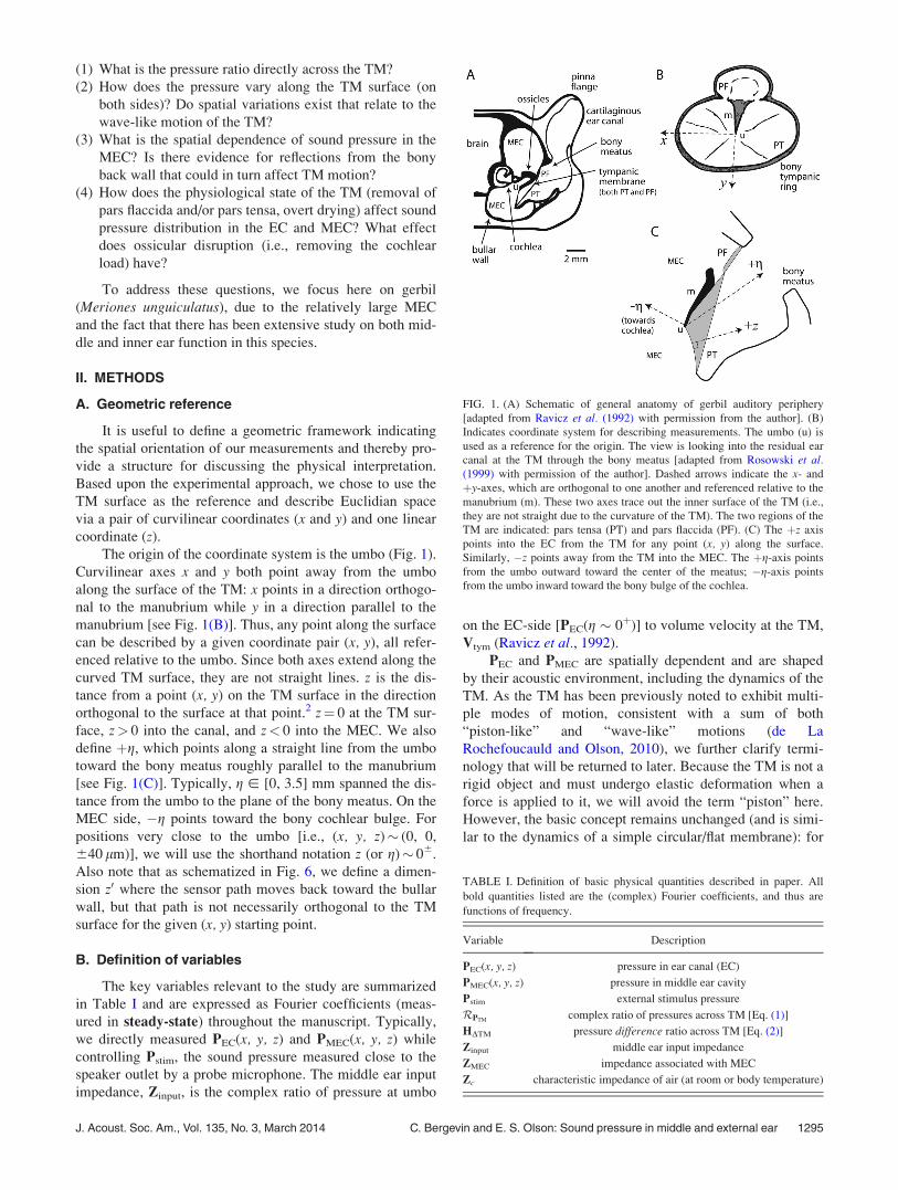
The origin of the coordinate system is the umbo (Fig. 1).

Curvilinear axes x and y both point away from the umbo

along the surface of the TM: x points in a direction orthogo-

nal to the manubrium while y in a direction parallel to the

manubrium [see Fig. 1(B)]. Thus, any point along the surface

can be described by a given coordinate pair (x, y), all refer-

enced relative to the umbo. Since both axes extend along the

curved TM surface, they are not straight lines. z is the dis-

tance from a point (x, y) on the TM surface in the direction

orthogonal to the surface at that point.2 z¼ 0 at the TM sur-

face, z> 0 into the canal, and z< 0 into the MEC. We also

define þg, which points along a straight line from the umbo

toward the bony meatus roughly parallel to the manubrium

[see Fig. 1(C)]. Typically, g � [0, 3.5] mm spanned the dis-

tance from the umbo to the plane of the bony meatus. On the

MEC side, �g points toward the bony cochlear bulge. For

positions very close to the umbo [i.e., (x, y, z)� (0, 0,

640 lm)], we will use the shorthand notation z (or g)� 06.

Also note that as schematized in Fig. 6, we define a dimen-

sion z0 where the sensor path moves back toward the bullar

wall, but that path is not necessarily orthogonal to the TM

surface for the given (x, y) starting point.

B. Definition of variables

The key variables relevant to the study are summarized

in Table I and are expressed as Fourier coefficients (meas-

ured in steady-state) throughout the manuscript. Typically,

we directly measured PEC(x, y, z) and PMEC(x, y, z) while

controlling Pstim, the sound pressure measured close to the

speaker outlet by a probe microphone. The middle ear input

impedance, Zinput, is the complex ratio of pressure at umbo

on the EC-side [PEC(g � 0þ)] to volume velocity at the TM,

Vtym (Ravicz et al., 1992).

PEC and PMEC are spatially dependent and are shaped

by their acoustic environment, including the dynamics of the

TM. As the TM has been previously noted to exhibit multi-

ple modes of motion, consistent with a sum of both

“piston-like” and “wave-like” motions (de La

Rochefoucauld and Olson, 2010), we further clarify termi-

nology that will be returned to later. Because the TM is not a

rigid object and must undergo elastic deformation when a

force is applied to it, we will avoid the term “piston” here.

However, the basic concept remains unchanged (and is simi-

lar to the dynamics of a simple circular/flat membrane): for

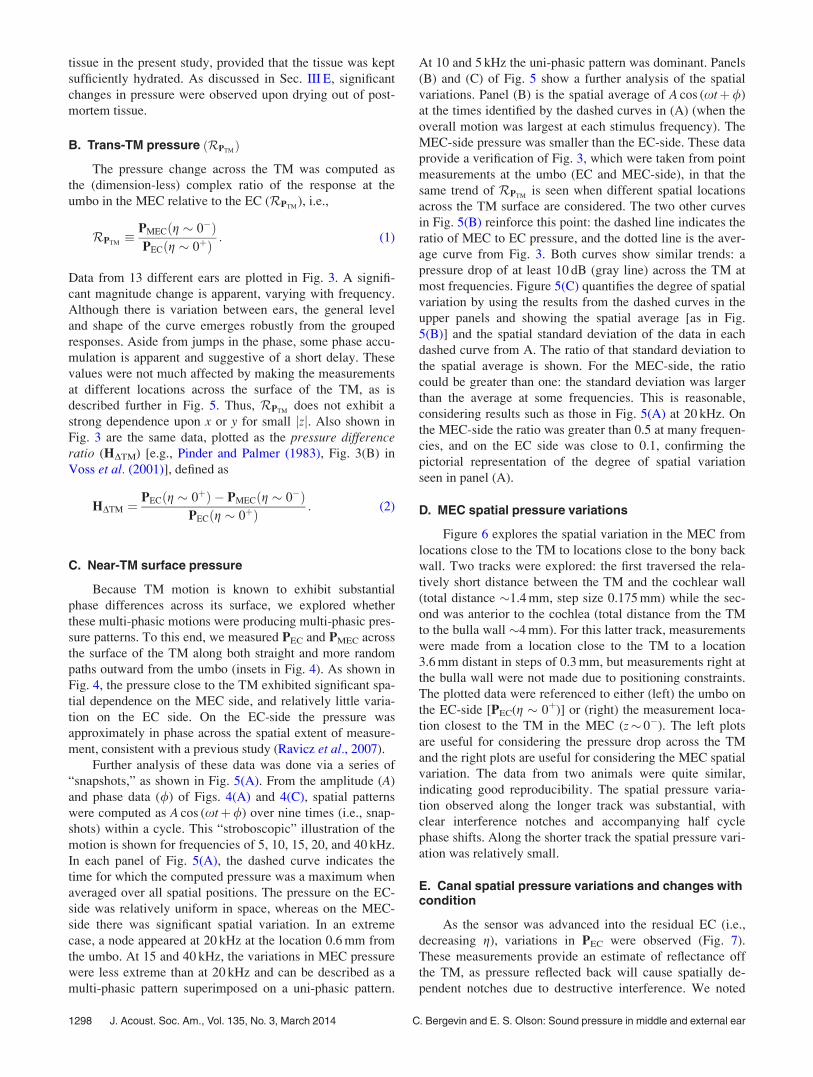
FIG. 1. (A) Schematic of general anatomy of gerbil auditory periphery

[adapted from Ravicz et al. (1992) with permission from the author]. (B)

Indicates coordinate system for describing measurements. The umbo (u) is

used as a reference for the origin. The view is looking into the residual ear

canal at the TM through the bony meatus [adapted from Rosowski et al.(1999) with permission of the author]. Dashed arrows indicate the x- and

þy-axes, which are orthogonal to one another and referenced relative to the

manubrium (m). These two axes trace out the inner surface of the TM (i.e.,

they are not straight due to the curvature of the TM). The two regions of the

TM are indicated: pars tensa (PT) and pars flaccida (PF). (C) The þz axis

points into the EC from the TM for any point (x, y) along the surface.

Similarly, �z points away from the TM into the MEC. The þg-axis points

from the umbo outward toward the center of the meatus; �g-axis points

from the umbo inward toward the bony bulge of the cochlea.

TABLE I. Definition of basic physical quantities described in paper. All

bold quantities listed are the (complex) Fourier coefficients, and thus are

functions of frequency.

Variable Description

PEC(x, y, z) pressure in ear canal (EC)

PMEC(x, y, z) pressure in middle ear cavity

Pstim external stimulus pressure

RPTMcomplex ratio of pressures across TM [Eq. (1)]

HDTM pressure difference ratio across TM [Eq. (2)]

Zinput middle ear input impedance

ZMEC impedance associated with MEC

Zc characteristic impedance of air (at room or body temperature)

J. Acoust. Soc. Am., Vol. 135, No. 3, March 2014 C. Bergevin and E. S. Olson: Sound pressure in middle and external ear 1295

lower frequency stimuli, when the whole TM moves in phase

in a simple in/out fashion this motion can be described as

uni-phasic. At higher frequencies, the motion becomes more

complicated and the motion can be described as multi-pha-sic.3 The multi-phasic case may stem from standing waves

and/or traveling waves along the TM surface.

C. Sound pressure measurements

Sound pressure was measured in two ways. First, a

probe tube microphone (Leonard, 1964; Sokolich, 1977) was

used that consisted of a 1/2 in. Br€uel & Kjær microphone

(type 4134, with a post amplifier type 2804) coupled with a

custom cover that allowed for connection of a �2.3 cm probe

tube with outer and inner diameters of 1.4 and 1.1 mm,

respectively. This assembly was calibrated via a custom en-

closure that allowed for a comparison to a separate 1/4 in.

Br€uel & Kjær microphone with known calibration and fre-

quency response. The factory-calibration of the 1/4 in. Br€uel

& Kjær microphone (type 4938) was confirmed using a

Br€uel & Kjær pistonphone at 1 kHz. Second, fiber-optic pres-

sure sensors were used (Olson, 1998) that allowed for inser-

tion into relatively small spaces given their dimensions

(�100 lm diameter). Each pressure sensor was calibrated

relative to the probe tube microphone both before and after

each experiment to ensure stability.4 A drawback of the sen-

sors was their sensitivity, as their noise floor (with a 1 Hz

bandwidth) is typically 50–60 dB sound pressure level

(SPL), flat across frequency. The sensor was positioned

using both a manual and motor-controlled micro-manipula-

tor. The latter allowed for steps as small as 1 lm, although

�12 lm steps were generally used. Placement very close to

the TM (within 10–20 lm) could be achieved by advancing

the sensor until it “tapped” the surface, then drawing back

one or two steps. This process did not damage the TM or

change the sensor sensitivity. The angle of incidence of the

sensor relative to the TM had no apparent effect upon the

measured pressure. Microphone signals were bandpass fil-

tered (PARC EG&G amplifier) between 0.01 and 300 kHz.

In order to make pressure measurements in the MEC, it

was necessary to open up the bulla cavity to some extent.

Additionally, for in vivo experiments, this was crucial to

allow a vent and thereby prevent a buildup of static pressure

in the MEC (presumably due to closure of the Eustachian

tube under anesthesia). While these holes were made as

small as possible, in some cases they needed to be substan-

tial (e.g., 1� 2 mm rectangle) to allow for sensor placement

over a sufficient range of locations. An acoustic baffle (via

clay) was placed between the acoustic assembly and the bul-

lar hole (see Fig. 2). This issue is discussed in more detail in

Sec. III G.

D. Acoustic stimulation

The majority of stimuli were presented in open-field, as

this allowed visual placement (via a surgical microscope) of

the sensor tip at various locations in the EC and MEC. The

acoustic source was a modified Radio Shack “Super-

Tweeter” speaker. The speaker was coupled to the probe

tube microphone via a short/flexible plastic tube and a

custom brass coupler such that the speaker and microphone

ports were at approximately the same location (see Fig. 2).

The acoustic assembly was typically placed �1–2 mm lateral

to the meatus. The stimulus sound level was calibrated insitu at the start and end of each experiment using flat-

spectrum random-phase noise. A variety of stimulus types

were used for the pressure measurements: single tones,

chirps, and noise. For the broadband stimuli, levels at the

probe tube microphone typically ranged from 50 to 90 dB

SPL, while for narrowband stimuli, 100 dB SPL tones were

used to ensure responses above the sensor noise floor. Pstim

was typically measured precisely via the probe tube micro-

phone (see Fig. 2), which could also be independently veri-

fied via the pressure sensor placed close to the microphone

port. The sound pressure at the plane of the meatus [i.e.,

PEC(g � 3.5 mm)] was approximately Pstim� 10 dB. The

speaker response was linear with respect to driving voltage

over the range used (70–110 dB SPL). Although broadband

and narrowband stimuli led to similar results, the majority of

data reported here are for tone stimuli so to maximize the

signal-to-noise ratio. A sampling rate of 195 kHz was used.

The uncertainty across the averaging period for a given mea-

surement (e.g., individual curves comprising Fig. 3) was

small in that responses could be repeated with typically less

than 1–2 dB change.

E. Animals

Measurements were made both in vivo and postmortem.

In some cases, postmortem measurements were necessary to

allow experimental access (e.g., exposure of the medial side

of the bulla wall). In other cases, postmortem measurements

were continued after the animal had been euthanized with

pentobarbital to examine changes in physiological state.

Based on our own experience, as long as the tissues remain

fresh and moist there is no apparent change in middle ear

transmission for many hours postmortem [e.g., de La

Rochefoucauld et al. (2008, 2010)]. The importance of keep-

ing the middle ear tissues moist is well known from the tem-

poral bone literature [e.g., Nakajima et al. (2005)].

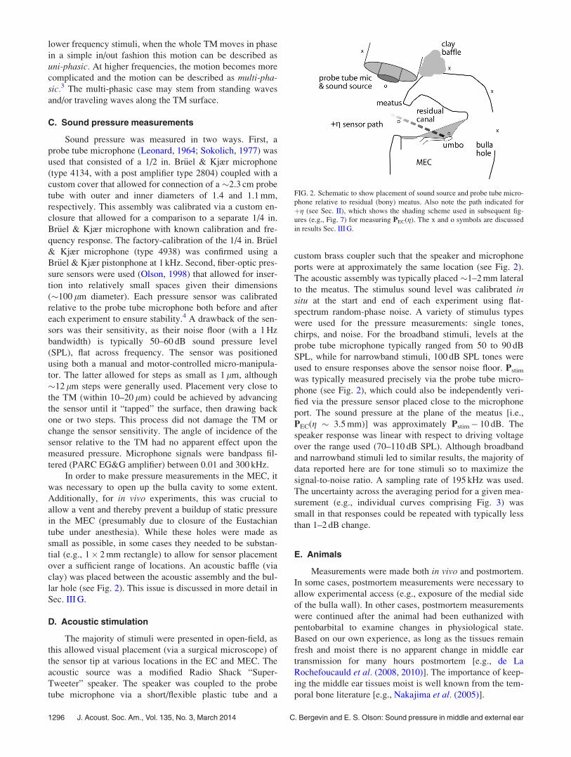
FIG. 2. Schematic to show placement of sound source and probe tube micro-

phone relative to residual (bony) meatus. Also note the path indicated for

þg (see Sec. II), which shows the shading scheme used in subsequent fig-

ures (e.g., Fig. 7) for measuring PEC(g). The x and o symbols are discussed

in results Sec. III G.

1296 J. Acoust. Soc. Am., Vol. 135, No. 3, March 2014 C. Bergevin and E. S. Olson: Sound pressure in middle and external ear

Thirty female adult gerbils (Meriones unguiculatus) were

used, some of these postmortem from other experiments. For

in vivo measurements, animals were dosed first with ketamine

to quiet the animal and then with sodium pentobarbital,

with redosing as needed based on toe pinch response.

Buprenorphine was administered as analgesic. Under anesthe-

sia the middle ear reflex is absent in gerbil (Schmiedt and

Zwislocki, 1977), so the middle ear muscles were left intact.

Following in vivo measurements, the animal was overdosed

with sodium pentobarbital. For postmortem data, measure-

ments were made either within several hours following death,

or the tissue was refrigerated in a moist paper towel and used

on a subsequent day. In those cases, the tissue was allowed to

come to room temperature and kept moist unless noted other-

wise. Unless noted otherwise, for all postmortem data the ear

was freshly exposed just prior to the start of the experiment

(i.e., the pinna was removed, tissue removed around the mea-

tus and bulla, and MEC opened). The pars tensa (parsT) and

ossicles were left intact, except for experiments where these

were purposely manipulated. In some experiments pars flac-

cida (parsF) was removed by penetrating and retracting it

with an insect pin that was bent at its tip. For disarticulation

(i.e., interruption of the incuo-stapedial joint), a fine needle

was inserted through the bulla hole to displace the ossicles.

Care was taken not to touch any other structure or put signifi-

cant tension upon the TM. Unless noted otherwise, all data

shown here are from temporal bones that were still embedded

in the head (i.e., not extracted). Animal use was approved by

the Columbia University IACUC.

F. Numerical simulations

Model computations were performed using Matlab, with

sufficient spectral resolution to identify notch depth visually.

III. RESULTS

A. Middle ear transmission

Several experiments were made early in the study to

characterize middle ear transmission (i.e., pressure just

inside the scala vestibuli near the stapes footplate relative to

pressure in the EC near the umbo) in order to verify reprodu-

cibility of that reported previously (Olson, 1998). While not

shown here, these experiments were consistent with that pre-

vious report, even for tissue that was several days postmor-

tem. This observation supported the use of postmortem

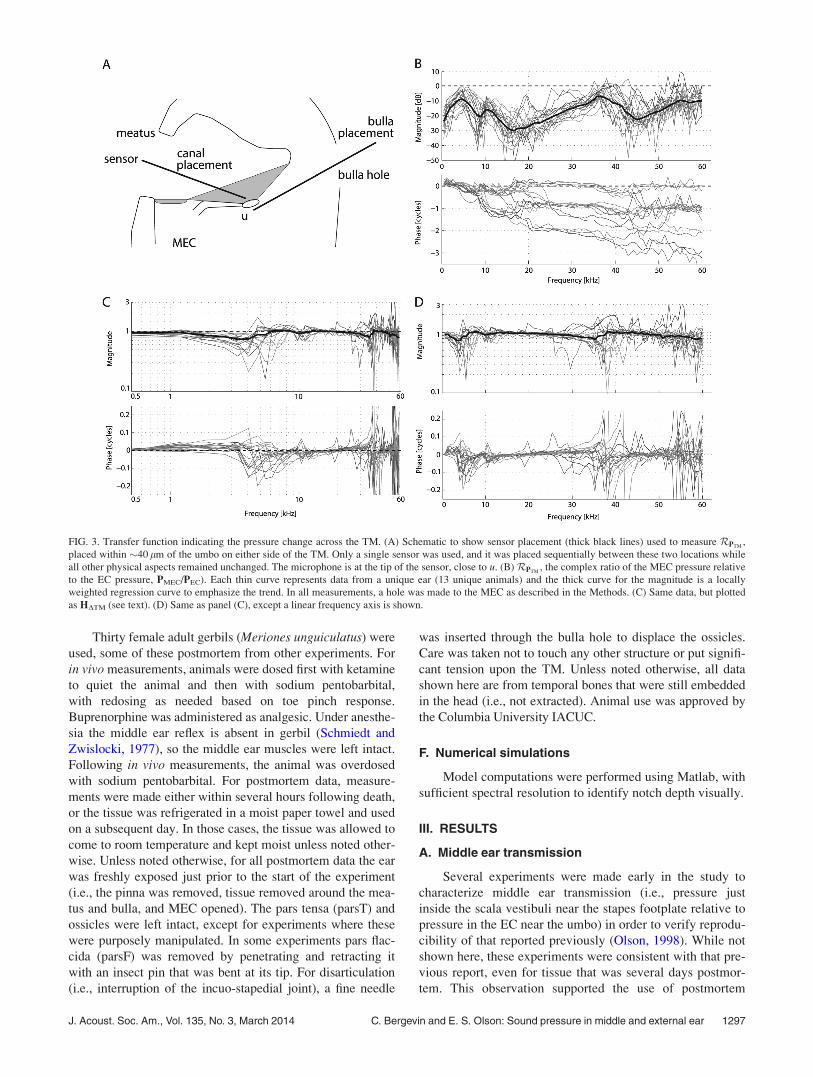
FIG. 3. Transfer function indicating the pressure change across the TM. (A) Schematic to show sensor placement (thick black lines) used to measure RPTM,

placed within �40 lm of the umbo on either side of the TM. Only a single sensor was used, and it was placed sequentially between these two locations while

all other physical aspects remained unchanged. The microphone is at the tip of the sensor, close to u. (B) RPTM, the complex ratio of the MEC pressure relative

to the EC pressure, PMEC/PEC). Each thin curve represents data from a unique ear (13 unique animals) and the thick curve for the magnitude is a locally

weighted regression curve to emphasize the trend. In all measurements, a hole was made to the MEC as described in the Methods. (C) Same data, but plotted

as HDTM (see text). (D) Same as panel (C), except a linear frequency axis is shown.


tissue in the present study, provided that the tissue was kept

sufficiently hydrated. As discussed in Sec. III E, significant

changes in pressure were observed upon drying out of post-

mortem tissue.

B. Trans-TM pressure RPTMð Þ

The pressure change across the TM was computed as

the (dimension-less) complex ratio of the response at the

umbo in the MEC relative to the EC (RPTM), i.e.,

RPTM� PMECðg � 0�Þ

PECðg � 0þÞ : (1)

Data from 13 different ears are plotted in Fig. 3. A signifi-

cant magnitude change is apparent, varying with frequency.

Although there is variation between ears, the general level

and shape of the curve emerges robustly from the grouped

responses. Aside from jumps in the phase, some phase accu-

mulation is apparent and suggestive of a short delay. These

values were not much affected by making the measurements

at different locations across the surface of the TM, as is

described further in Fig. 5. Thus, RPTMdoes not exhibit a

strong dependence upon x or y for small jzj. Also shown in

Fig. 3 are the same data, plotted as the pressure differenceratio (HDTM) [e.g., Pinder and Palmer (1983), Fig. 3(B) in

Voss et al. (2001)], defined as

HDTM ¼PECðg � 0þÞ � PMECðg � 0�Þ

PECðg � 0þÞ : (2)

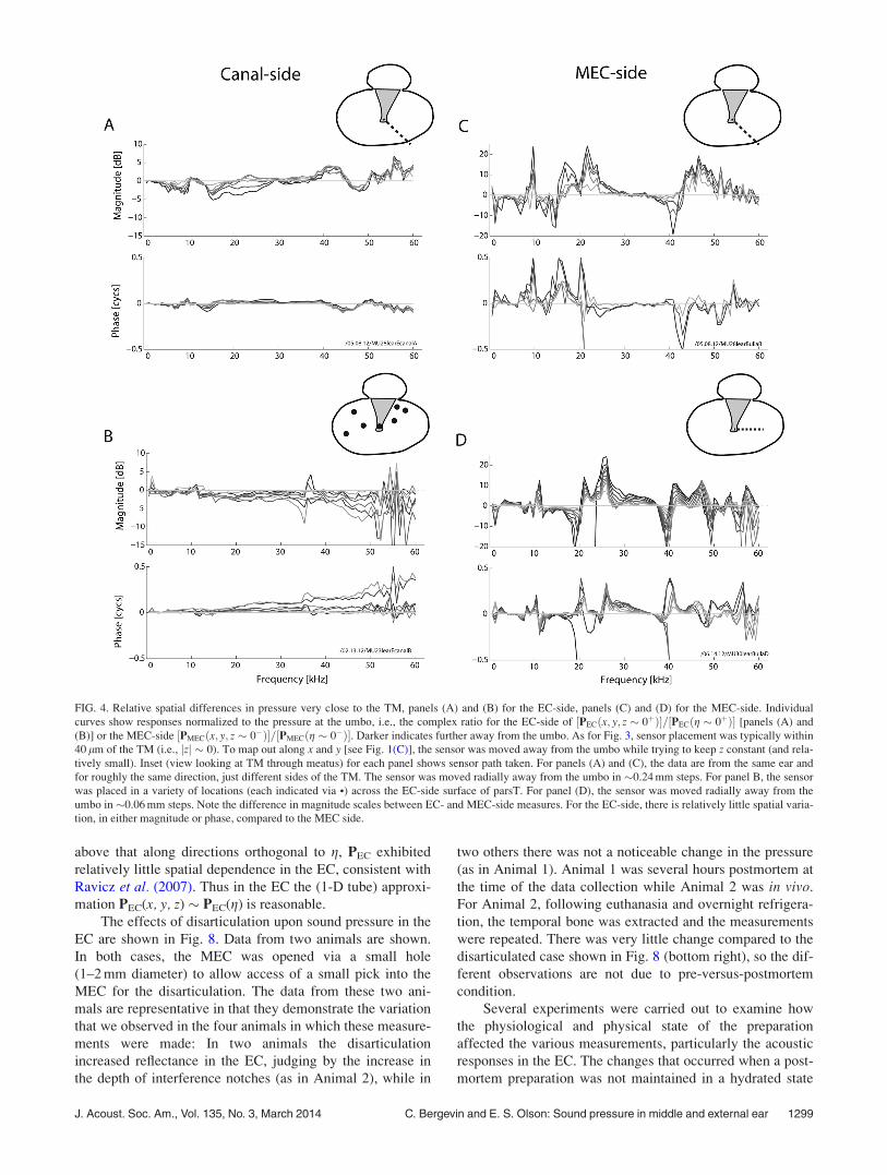
C. Near-TM surface pressure

Because TM motion is known to exhibit substantial

phase differences across its surface, we explored whether

these multi-phasic motions were producing multi-phasic pres-

sure patterns. To this end, we measured PEC and PMEC across

the surface of the TM along both straight and more random

paths outward from the umbo (insets in Fig. 4). As shown in

Fig. 4, the pressure close to the TM exhibited significant spa-

tial dependence on the MEC side, and relatively little varia-

tion on the EC side. On the EC-side the pressure was

approximately in phase across the spatial extent of measure-

ment, consistent with a previous study (Ravicz et al., 2007).

Further analysis of these data was done via a series of

“snapshots,” as shown in Fig. 5(A). From the amplitude (A)

and phase data (/) of Figs. 4(A) and 4(C), spatial patterns

were computed as A cos (xtþ/) over nine times (i.e., snap-

shots) within a cycle. This “stroboscopic” illustration of the

motion is shown for frequencies of 5, 10, 15, 20, and 40 kHz.

In each panel of Fig. 5(A), the dashed curve indicates the

time for which the computed pressure was a maximum when

averaged over all spatial positions. The pressure on the EC-

side was relatively uniform in space, whereas on the MEC-

side there was significant spatial variation. In an extreme

case, a node appeared at 20 kHz at the location 0.6 mm from

the umbo. At 15 and 40 kHz, the variations in MEC pressure

were less extreme than at 20 kHz and can be described as a

multi-phasic pattern superimposed on a uni-phasic pattern.

At 10 and 5 kHz the uni-phasic pattern was dominant. Panels

(B) and (C) of Fig. 5 show a further analysis of the spatial

variations. Panel (B) is the spatial average of A cos (xtþ/)

at the times identified by the dashed curves in (A) (when the

overall motion was largest at each stimulus frequency). The

MEC-side pressure was smaller than the EC-side. These data

provide a verification of Fig. 3, which were taken from point

measurements at the umbo (EC and MEC-side), in that the

same trend of RPTMis seen when different spatial locations

across the TM surface are considered. The two other curves

in Fig. 5(B) reinforce this point: the dashed line indicates the

ratio of MEC to EC pressure, and the dotted line is the aver-

age curve from Fig. 3. Both curves show similar trends: a

pressure drop of at least 10 dB (gray line) across the TM at

most frequencies. Figure 5(C) quantifies the degree of spatial

variation by using the results from the dashed curves in the

upper panels and showing the spatial average [as in Fig.

5(B)] and the spatial standard deviation of the data in each

dashed curve from A. The ratio of that standard deviation to

the spatial average is shown. For the MEC-side, the ratio

could be greater than one: the standard deviation was larger

than the average at some frequencies. This is reasonable,

considering results such as those in Fig. 5(A) at 20 kHz. On

the MEC-side the ratio was greater than 0.5 at many frequen-

cies, and on the EC side was close to 0.1, confirming the

pictorial representation of the degree of spatial variation

seen in panel (A).

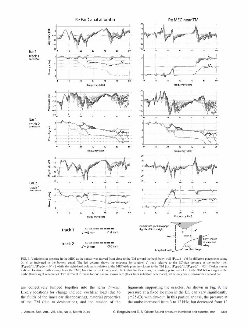
D. MEC spatial pressure variations

Figure 6 explores the spatial variation in the MEC from

locations close to the TM to locations close to the bony back

wall. Two tracks were explored: the first traversed the rela-

tively short distance between the TM and the cochlear wall

(total distance �1.4 mm, step size 0.175 mm) while the sec-

ond was anterior to the cochlea (total distance from the TM

to the bulla wall �4 mm). For this latter track, measurements

were made from a location close to the TM to a location

3.6 mm distant in steps of 0.3 mm, but measurements right at

the bulla wall were not made due to positioning constraints.

The plotted data were referenced to either (left) the umbo on

the EC-side [PEC(g � 0þ)] or (right) the measurement loca-

tion closest to the TM in the MEC (z� 0�). The left plots

are useful for considering the pressure drop across the TM

and the right plots are useful for considering the MEC spatial

variation. The data from two animals were quite similar,

indicating good reproducibility. The spatial pressure varia-

tion observed along the longer track was substantial, with

clear interference notches and accompanying half cycle

phase shifts. Along the shorter track the spatial pressure vari-

ation was relatively small.

E. Canal spatial pressure variations and changes withcondition

As the sensor was advanced into the residual EC (i.e.,

decreasing g), variations in PEC were observed (Fig. 7).

These measurements provide an estimate of reflectance off

the TM, as pressure reflected back will cause spatially de-

pendent notches due to destructive interference. We noted


above that along directions orthogonal to g, PEC exhibited

relatively little spatial dependence in the EC, consistent with

Ravicz et al. (2007). Thus in the EC the (1-D tube) approxi-

mation PEC(x, y, z) � PEC(g) is reasonable.

The effects of disarticulation upon sound pressure in the

EC are shown in Fig. 8. Data from two animals are shown.

In both cases, the MEC was opened via a small hole

(1–2 mm diameter) to allow access of a small pick into the

MEC for the disarticulation. The data from these two ani-

mals are representative in that they demonstrate the variation

that we observed in the four animals in which these measure-

ments were made: In two animals the disarticulation

increased reflectance in the EC, judging by the increase in

the depth of interference notches (as in Animal 2), while in

two others there was not a noticeable change in the pressure

(as in Animal 1). Animal 1 was several hours postmortem at

the time of the data collection while Animal 2 was in vivo.

For Animal 2, following euthanasia and overnight refrigera-

tion, the temporal bone was extracted and the measurements

were repeated. There was very little change compared to the

disarticulated case shown in Fig. 8 (bottom right), so the dif-

ferent observations are not due to pre-versus-postmortem

condition.

Several experiments were carried out to examine how

the physiological and physical state of the preparation

affected the various measurements, particularly the acoustic

responses in the EC. The changes that occurred when a post-

mortem preparation was not maintained in a hydrated state

FIG. 4. Relative spatial differences in pressure very close to the TM, panels (A) and (B) for the EC-side, panels (C) and (D) for the MEC-side. Individual

curves show responses normalized to the pressure at the umbo, i.e., the complex ratio for the EC-side of ½PECðx; y; z � 0þÞ�=½PECðg � 0þÞ� [panels (A) and

(B)] or the MEC-side ½PMECðx; y; z � 0�Þ�=½PMECðg � 0�Þ�. Darker indicates further away from the umbo. As for Fig. 3, sensor placement was typically within

40 lm of the TM (i.e., jzj � 0). To map out along x and y [see Fig. 1(C)], the sensor was moved away from the umbo while trying to keep z constant (and rela-

tively small). Inset (view looking at TM through meatus) for each panel shows sensor path taken. For panels (A) and (C), the data are from the same ear and

for roughly the same direction, just different sides of the TM. The sensor was moved radially away from the umbo in �0.24 mm steps. For panel B, the sensor

was placed in a variety of locations (each indicated via •) across the EC-side surface of parsT. For panel (D), the sensor was moved radially away from the

umbo in �0.06 mm steps. Note the difference in magnitude scales between EC- and MEC-side measures. For the EC-side, there is relatively little spatial varia-

tion, in either magnitude or phase, compared to the MEC side.


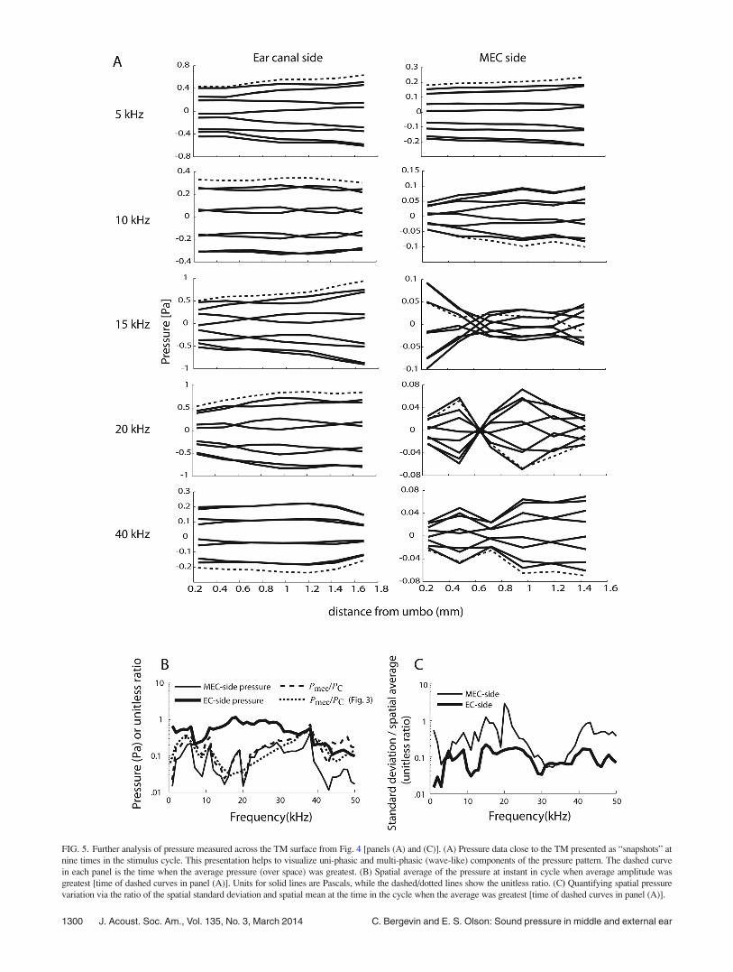
FIG. 5. Further analysis of pressure measured across the TM surface from Fig. 4 [panels (A) and (C)]. (A) Pressure data close to the TM presented as “snapshots” at

nine times in the stimulus cycle. This presentation helps to visualize uni-phasic and multi-phasic (wave-like) components of the pressure pattern. The dashed curve

in each panel is the time when the average pressure (over space) was greatest. (B) Spatial average of the pressure at instant in cycle when average amplitude was

greatest [time of dashed curves in panel (A)]. Units for solid lines are Pascals, while the dashed/dotted lines show the unitless ratio. (C) Quantifying spatial pressure

variation via the ratio of the spatial standard deviation and spatial mean at the time in the cycle when the average was greatest [time of dashed curves in panel (A)].


are collectively lumped together into the term dry-out.Likely locations for change include: cochlear load (due to

the fluids of the inner ear disappearing), material properties

of the TM (due to desiccation), and the tension of the

ligaments supporting the ossicles. As shown in Fig. 9, the

pressure at a fixed location in the EC can vary significantly

(625 dB) with dry-out. In this particular case, the pressure at

the umbo increased from 3 to 12 kHz, but decreased from 12

FIG. 6. Variations in pressure in the MEC as the sensor was moved from close to the TM toward the back bony wall [PMEC(�z0)] for different placements along

(x, y) as indicated in the bottom panel. The left column shows the response for a given z0 track relative to the EC-side pressure at the umbo {i.e.,

½PMECðz0Þ�=½PECðg � 0þÞ�} while the right-hand column is relative to the MEC-side pressure closest to the TM {i.e., ½PMECðz0Þ�=½PMECðz0 ¼ 0Þ�}. Darker curves

indicate locations further away from the TM (closer to the back bony wall). Note that for these runs, the starting point was close to the TM but not right at the

umbo (lower right schematic). Two different z0 tracks for one ear are shown here (thick lines in bottom schematic), while only one is shown for a second ear.


to 30 kHz (as if a notch developed, whose frequency shifted

upward with time). This effect evolved smoothly as time

progressed. Thus, the physiological state of the TM had a

strong effect upon the pressure in the canal.

To better understand how changes in material properties

could affect the acoustical responses, further postmortem

experiments examined the effects due to dry-out after a suit-

ably long amount of time had passed to allow for responses

to stabilize. A period of 24 h at room temperature appeared

sufficient to attain a reasonably fully dried out state. In such

a state, there was relatively little change in jPMECðg � 0�Þjabove 10 kHz before and after removal of the TM. The effect

of changes in the EC spatial profile were measured (Fig. 10,

left column), as was the subsequent effect of ossicular dis-

ruption (right column). Compared to the viable condition

(Fig. 8), not only is the overall profile substantially different

in the dried-out condition, but so is the effect of disarticula-

tion, such that the patterns of reflected sound changed sub-

stantially upon removal of the cochlear/ossicular load.

F. Pars flaccida removal

Given that several previous studies have removed the

parsF [e.g., de La Rochefoucauld and Olson (2010)],

typically to allow access to the stapes or cochlea, we

explored how such an opening affected the pressure at the

TM. In the top panels of Fig. 11 we show data similar to

that of Fig. 3, on the left as the ratio RPTMand on the right

the pressure difference ratio HDTM. Results from two prepa-

rations are shown [Figs. 3(A) and 3(B)]. Both exhibit a

5–10 dB increase in RPTMat frequencies below �20 kHz,

with relatively random variations at higher frequencies (left

upper panels). However, the phases of PMEC and Pstim tend

to be different, so the pressure difference remains substan-

tial even when these magnitudes are similar. This can be

seen in the right panels, where HDTM remains close to 1 fol-

lowing removal of parsF (right upper panels). In preparation

A the removal caused �4 dB decrease in the pressure dif-

ference ratio up to 2.5 kHz, and then a slightly larger dip at

�4 kHz. Above 6 kHz, there was no significant difference

in HDTM before and after removal of parsF. The preparation

of panel B showed a larger decrease in the HDTM at fre-

quencies from 2 to 6 kHz, but like the preparation of panel

A, above 6 kHz the changes were small. The bottom plots

of panels (A) and (B) of Fig. 11 show that parsF removal

had relatively little effect upon the reflectance, in that the

depth of interference notches did not change substantially

or systematically.

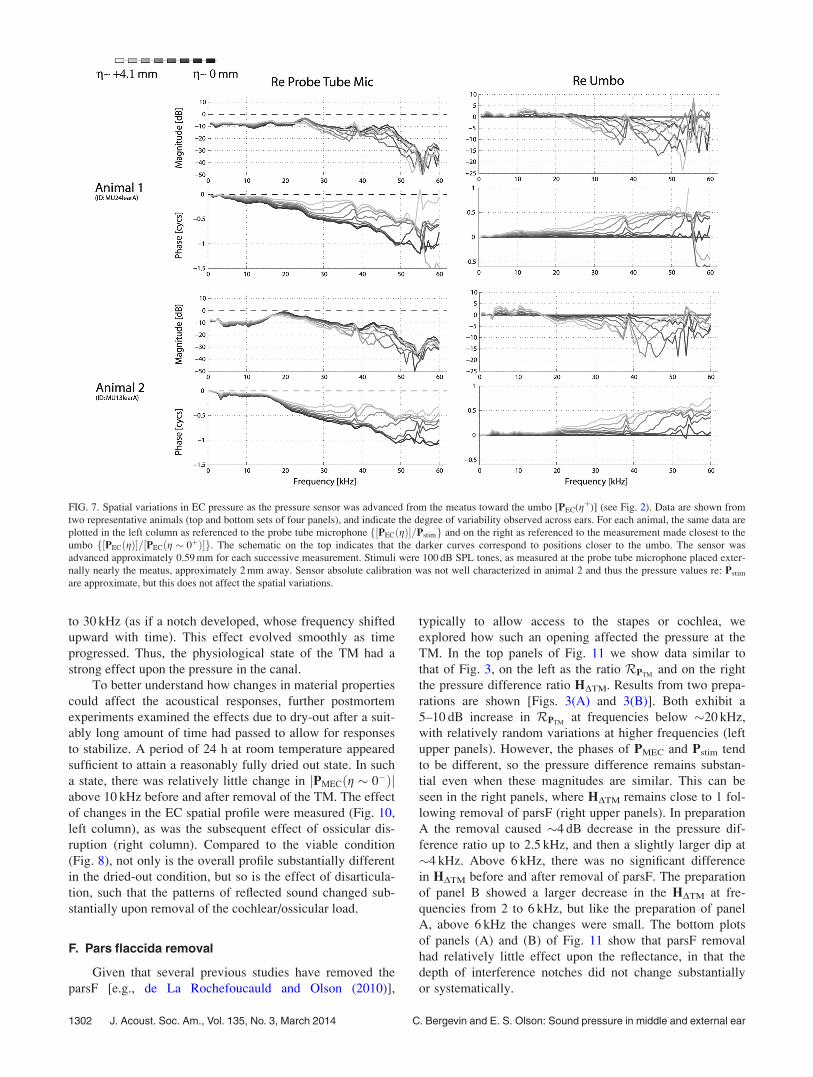
FIG. 7. Spatial variations in EC pressure as the pressure sensor was advanced from the meatus toward the umbo [PEC(gþ)] (see Fig. 2). Data are shown from

two representative animals (top and bottom sets of four panels), and indicate the degree of variability observed across ears. For each animal, the same data are

plotted in the left column as referenced to the probe tube microphone f½PECðgÞ�=Pstimg and on the right as referenced to the measurement made closest to the

umbo f½PECðgÞ�=½PECðg � 0þÞ�g. The schematic on the top indicates that the darker curves correspond to positions closer to the umbo. The sensor was

advanced approximately 0.59 mm for each successive measurement. Stimuli were 100 dB SPL tones, as measured at the probe tube microphone placed exter-

nally nearly the meatus, approximately 2 mm away. Sensor absolute calibration was not well characterized in animal 2 and thus the pressure values re: Pstim

are approximate, but this does not affect the spatial variations.


G. Additional observations

1. Pars tensa removal and reverse TM stimulation viabullar hole

An important control question was to what extent open-

ing the MEC cavity created an additional sound pathway:

Was the TM also being significantly driven from the MEC-

side by Pstim due to the bulla hole? Such a question was par-

ticularly relevant for experiments where the MEC had to be

opened sufficiently to allow for sensor placement at a variety

of locations in the MEC (�1� 2 mm rectangular hole). This

question was explored in a number of ways, including: (1)

Adding in/removing the clay baffle (see Fig. 2), (2) Sealing

the hole with clay (both for the sensor inside and outside the

bulla), (3) Mapping out the pressure distribution (with the

sensor) as it was moved away from the source around the

bulla toward the hole, (4) Mapping the pressure in the bulla

as the sensor was pulled out of the hole, (5) Observing the

change in the bulla pressure as the meatus (EC opening) and

or sound source was plugged/unplugged, (6) Observing the

effect upon both canal and bulla pressure when the TM (both

parsF and parsT) was removed, and (7) Making smaller

holes to the MEC wall.5

These manipulations led to the following observations:

First, upon plugging the bulla hole with clay, PEC was little

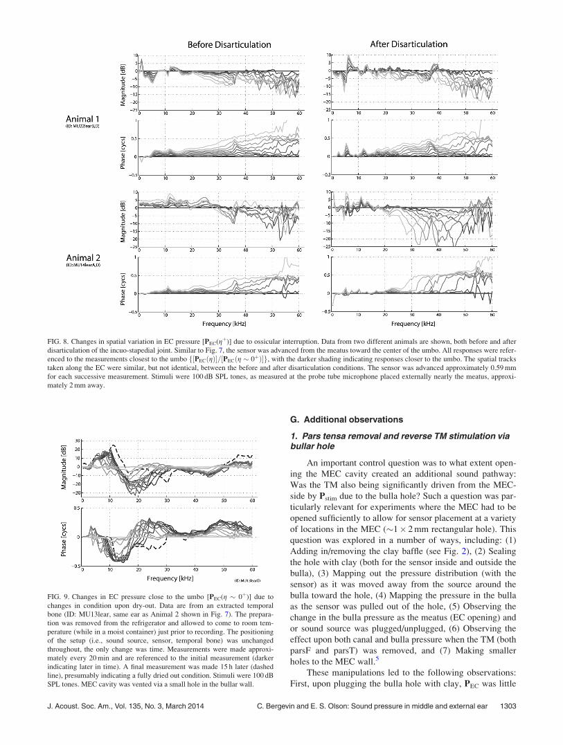
FIG. 9. Changes in EC pressure close to the umbo [PEC(g � 0þ)] due to

changes in condition upon dry-out. Data are from an extracted temporal

bone (ID: MU13lear, same ear as Animal 2 shown in Fig. 7). The prepara-

tion was removed from the refrigerator and allowed to come to room tem-

perature (while in a moist container) just prior to recording. The positioning

of the setup (i.e., sound source, sensor, temporal bone) was unchanged

throughout, the only change was time. Measurements were made approxi-

mately every 20 min and are referenced to the initial measurement (darker

indicating later in time). A final measurement was made 15 h later (dashed

line), presumably indicating a fully dried out condition. Stimuli were 100 dB

SPL tones. MEC cavity was vented via a small hole in the bullar wall.

FIG. 8. Changes in spatial variation in EC pressure [PEC(gþ)] due to ossicular interruption. Data from two different animals are shown, both before and after

disarticulation of the incuo-stapedial joint. Similar to Fig. 7, the sensor was advanced from the meatus toward the center of the umbo. All responses were refer-

enced to the measurements closest to the umbo f½PECðgÞ�=½PECðg � 0þÞ�g, with the darker shading indicating responses closer to the umbo. The spatial tracks

taken along the EC were similar, but not identical, between the before and after disarticulation conditions. The sensor was advanced approximately 0.59 mm

for each successive measurement. Stimuli were 100 dB SPL tones, as measured at the probe tube microphone placed externally nearly the meatus, approxi-

mately 2 mm away.


affected for frequencies above 5 kHz except for occasional

small frequency shifts in the peaks/valleys.6 However in one

case where these measurements were made following disar-

ticulation, there was a slight downward shift and accentua-

tion of spectral structure for frequencies below about 7 kHz

only (no effect at higher frequencies). Second, thoroughly

plugging the meatus had a drastic effect upon the MEC pres-

sure (PMEC) and caused the response to drop down into the

noise floor above 10 kHz. Third, the effect of adding or

removing a clay baffle (Fig. 2) had relatively little effect

upon RPTM. Fourth, the sound pressure distribution measured

at various locations about the preparation (see Fig. 2) indi-

cate that the sound field falls off steeply away from the

source (x symbols) but is relatively uniform about the mea-

tus and into the EC close to the umbo (o symbols). Thus it

appears that most of the relevant acoustic stimulus energy

enters into the EC rather than leaking back around through

the bullar wall hole. In fact, what little sound pressure was

measurable just outside the hole appeared to be coming from

the MEC (i.e., through the EC and TM) and radiating out-

ward from the hole. Last, while the sound pressure was fairly

uniform throughout the residual EC when the TM was in its

normal physiological state, removal of the TM drastically

changed PEC, in particular, producing large notches. Large

holes in parsT (but umbo/manubrium still in place) produced

similar effects as total TM removal. When placed close to

where the umbo had been, PEC(g � 0þ) appeared highly sim-

ilar to PMEC(g � 0�) for the intact condition. PMEC was

relatively little changed upon TM removal, such that jHDTMjbecame vanishingly small (which was to be expected in the

absence of the TM).

2. Modifying ear canal shape

Aside from the frequency/spatial-dependent notch appa-

rent for many (but not all) ears, the pressure was fairly uni-

form in the EC as the sensor was advanced from the meatus

toward the umbo [i.e., PEC(gþ) as shown in Fig. 7]. One

question was whether this depended crucially upon the ge-

ometry of the EC. To test this, a small amount of clay was

carefully placed along the bony wall opposite the TM (where

the curved shape shown in panel C of Fig. 1 suggests focus-

ing) leaving enough room to advance the sensor along the

path toward the umbo unimpeded. The clay modified the

shape of the EC (taking up �30% of the volume), but did

not touch the TM. When the clay was in place the location

of various peaks and valleys shifted downward with fre-

quency by as much as 10 kHz, but otherwise the change was

small.7

IV. DISCUSSION

This paper explores several questions aimed at better

understanding how sound pressure sets the TM into motion

and thereby efficiently delivers energy to the inner ear. We

concentrate the discussion upon several salient observations

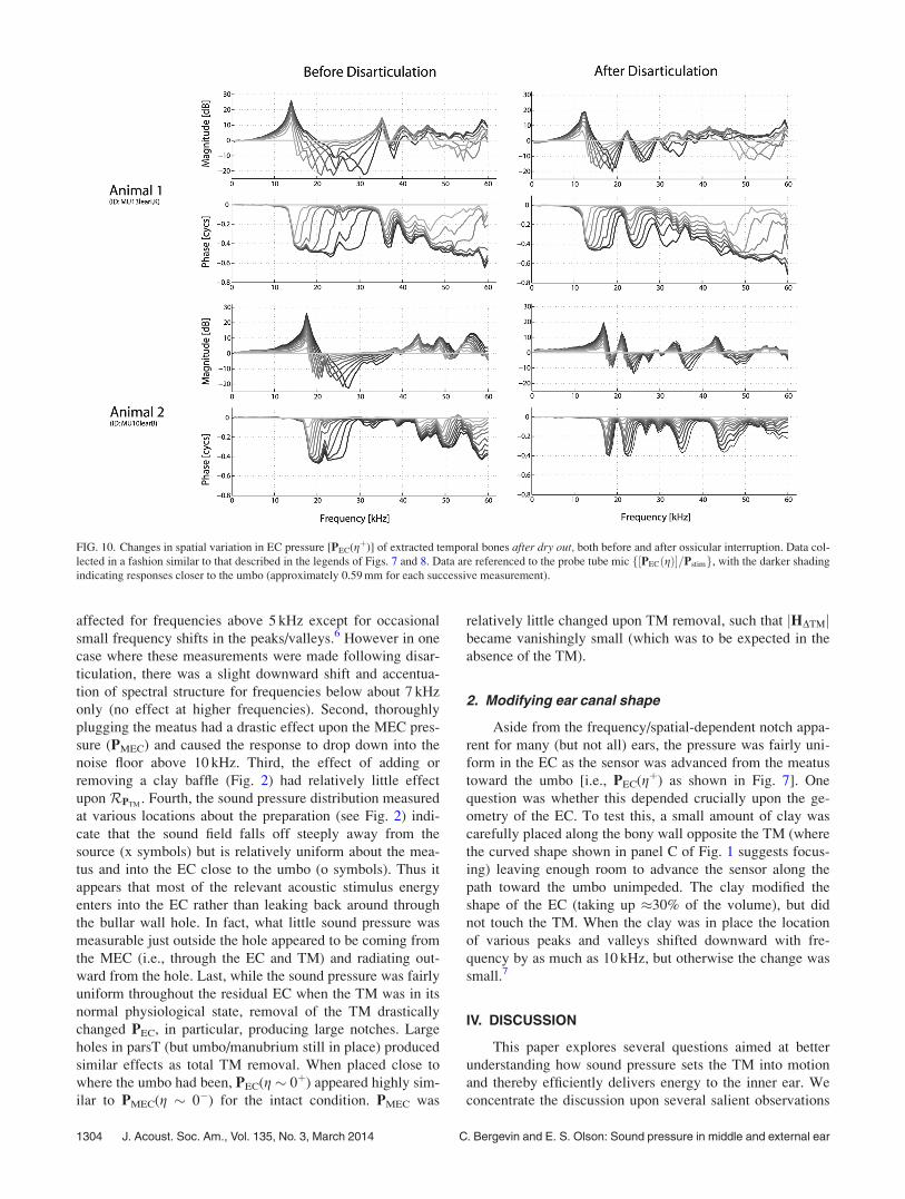
FIG. 10. Changes in spatial variation in EC pressure [PEC(gþ)] of extracted temporal bones after dry out, both before and after ossicular interruption. Data col-

lected in a fashion similar to that described in the legends of Figs. 7 and 8. Data are referenced to the probe tube mic f½PECðgÞ�=Pstimg, with the darker shading

indicating responses closer to the umbo (approximately 0.59 mm for each successive measurement).


FIG. 11. Effects of removing pars flaccida (parsF). Results are shown for two different ears, one in vivo (A) and the other postmortem that had been refriger-

ated for two weeks (B). For each ear, four panels are shown. In the top two, the trans-TM pressure is shown in a fashion similar to that in Figs. 3(A) and 3(B),

RPTMon the left and HDTM on the right, with intact-parsF case indicated via a solid line and removed-parsF shown by the dashed line. The bottom sets of pan-

els show the spatial variation in canal pressure (similar to Fig. 7, referenced to the umbo), the left for intact-parsF and the right for the parsF removed. Darker

shading indicates closer to the umbo.


emerging from the data, initially providing a brief overview

of the relevant anatomy.

A. Overview of gerbil middle ear anatomy

Several previous reports provide detailed descriptions

and schematics of the gerbil external and middle ear mor-

phology and mechanics (Ravicz et al., 1992; Rosowski

et al., 1999; Ravicz et al., 2007). We note several features

relevant to the discussion. First, the EC (upon removal of the

pinna and soft tissue about the external auditory meatus) is a

cavity in which the TM is not simply the termination of the

end of a tube. Instead, the TM covers a substantial fraction

of the EC’s surface area along one side, the other side taper-

ing down (see Fig. 1) so to perhaps focus sound pressure at

the TM surface along its semi-conical shape. Second, it

should be noted that there are considerable differences in the

morphology of the external ears of humans and gerbils (e.g.,

EC length and shape, relative size of parsF versus parsT).

Thus, one needs to be careful when considering the present

results in the context of human hearing. Lastly, the TM itself

appears as an extremely light and fragile structure, giving

rise to an expectation that it will undergo significant motion

when driven with pressure and thereby generate substantial

pressure on the MEC side (Rabbitt, 1990).

B. Spatial variations along ear canal

Figures 7 and 8 show the spatial variation of PEC and

indicate the existence of spatially dependent notches (i.e.,

areas of destructive interference between forward- and

reverse-traveling waves). These data can be directly related

to previous studies such as Stinson (1985) and Ravicz et al.(2007). The latter study reported interference notches at fre-

quencies above about 30 kHz, with dips that varied from 10

to 25 dB. Some preparations showed deeper notches (indicat-

ing greater reflection) and the variability across ears was

apparent in the factor of three range in power reflectance

[see Fig. 13 of Ravicz et al. (2007)]. The notches reported

here are reasonably similar to the results of Ravicz et al.(2007), but some preparations exhibited relatively shallow

notches (e.g., less than 10 dB up to 45 kHz, Fig. 8 upper

left). It is not known why the results of the two studies differ

somewhat in PEC notch depth—Ravicz et al. (2007) used

both probe tube microphones and micro-pressure sensors

similar to those in the current report, and studied both pre-

and post-mortem ears. It is possible that the fairly small

number of preparations in both reports simply was not

enough to fully characterize the range of reflectance values

across different gerbil ears.

C. Pressure ratio across TM (RPTM)

Our results for RPTMindicate a significant drop in pres-

sure across the TM. These results are consistent with previ-

ous studies [e.g., Rosowski and Saunders (1980); Pinder and

Palmer (1983); Voss et al. (2001)], which reported that

jHDTMj � 1 (especially above 1 kHz). While Fig. 3 shows

this ratio can be smaller at certain frequencies (e.g., 5, 40,

and 55 kHz) and that individual curves can depart

significantly from the trend (e.g., RPTMbeing close to or

greater than 1 in several cases), jRPTMj when averaged across

animals was always at least 7 dB down. Figure 5 shows that

the jRPTMj averaged over several locations on the TM in a

single preparation similarly was always less than one and

usually down by a factor of three or more. While most meas-

urements of RPTMwere made across the umbo, the general

features were little changed when measuring across the TM

for different locations along parsT.

The frequency-dependent features of jRPTMj (Fig. 3) do

not match the relatively flat middle ear transmission found

with intracochlear pressure measurements [e.g., Olson

(1998); Dong and Olson (2006)]. However, the pressure dif-

ference across the TM is the quantity driving the TM, not the

pressure ratio and HDTM [Figs. 3(C) and 3(D)] is the more

important quantity to consider in this regard. HDTM it is quite

flat with frequency, which does match the relatively flat

transmission observed in other studies. These observations

underscore that the relatively large value of jRPTMj indicates

that the pressure drive to the TM is well approximated by

PEC(g � 0þ).

The phase data shown in Fig. 3 are suggestive of a delay

between PMEC and PEC. The RPTMphase does not impact

transmission in an obvious way, since as noted above, to a

good approximation the drive to the TM is PEC(g � 0þ).

Nevertheless, it is interesting that the delay between PMEC

and PEC is on the order of tens of microseconds, similar to

that of the documented TM transmission: in gerbil the lag of

intracochlear pressure (just inside the stapes footplate) rela-

tive to PEC is �25–30 ls, independent of frequency [e.g.,

Olson (1998); Dong and Olson (2006)]. While a fraction of

the forward transmission delay appears attributable to the

ossicles (de La Rochefoucauld et al., 2010), the majority

may arise at the TM. The source of TM delay has been

explored in previous work, but a clear understanding has yet

to emerge (Puria and Allen, 1998; Fay et al., 2006; Parent

and Allen, 2007; de La Rochefoucauld and Olson, 2010;

Goll and Dalhoff, 2011). For example, delays could arise via

(relatively) slow-moving inward-traveling waves that carry

energy from the outer edges in toward the center where the

umbo attaches to the TM (although delays measured along

the gerbil manubrium indicated motion propagation outwardfrom the umbo to the lateral process of the malleus [de La

Rochefoucauld et al. (2010)]. TM traveling waves may be

present in other types of tympanums such as those of frogs,

where middle ear transmission delays can be substantially

longer than those of mammals [0.7 ms; van Dijk et al.(2011)]. A recent theoretical study examined a relationship

between delays associated with both transmission and TM

surface waves and suggested the two could be independent

of one another (Goll and Dalhoff, 2011). Section 1 of model-

ing Sec. IV G attempts to provide an explanation concerning

several aspects ofRPTM.

D. Pressure distribution along TM surface

Previous studies have demonstrated complicated spatial

variations in displacement across the TM surface of mam-

mals (Khanna and Tonndorf, 1972; Decraemer et al., 1989;


Furlong et al., 2009; Rosowski et al., 2013), as well as non-

mammals [Pinder and Palmer (1983); Manley (1972)]. It has

been suggested that this motion is a combination of uni- and

multi-phasic motion patterns (de La Rochefoucauld and

Olson, 2010). While TM velocity was not measured in the

current study, pressure variations close to the surface were

examined on both sides of the TM. By and large, the spatial

variation on the EC-side was small, indicating that multi-

phasic motion of the TM did not influence the pressure field

very much, even as close as 40 lm to the TM. Apparently

the pressure produced by the multi-phasic motion of the TM

was only a small perturbation to the stimulating pressure.

These results are consistent with previous measurements

made by Ravicz et al. (2007).

In contrast, significant spatial variations in pressure

were apparent along the TM surface on the MEC-side, and

wave-like spatial pressure patterns are illustrated in Fig. 5.

The pressure in the MEC is produced by the motion of the

TM, which has a prominent multi-phasic component.

Therefore, it was not surprising that the PMEC(x, y, z � 0�)

also would have a multi-phasic character. Recognizing that

motion of the TM will produce MEC pressure, a further

question was whether reflection of this pressure off the back

cavity walls was large enough to significantly modify the

MEC pressure at the TM, and thus augment or diminish the

pressure difference across the TM that drives its motion.

This question is addressed in the next section.

E. MEC acoustics

Rabbitt (1990) hypothesized that reflections in the MEC

provide an additional drive to TM motion and thus extend

high frequency sensitivity, and our observations of MEC

pressure variations speak to this notion. For track 1 in Fig. 6,

standing wave patterns (i.e., pressure minima accompanied

by half-cycle phase shifts) were not in evidence. While there

are regions where notches appeared, the degree of the associ-

ated phase shifts were variable in size. One likely explana-

tion is that given the distance of 1.4 mm corresponds to a

quarter wave of frequency 61 kHz, standing waves would

not be observed over the relatively short track 1. It also must

be considered that because the MEC is not a simple 1-D

tube, but a more complex 3-D cavity, the “classic” standing

wave expectation may be too simple [e.g., consider an arbi-

trary position in/track through a spherical 3-D geometry,

Russell (2010)].

Track 2 expands upon these reasonings: with a total dis-

tance of 5 mm, quarter-wave standing wave patterns would

emerge at a frequency of �17 kHz and indeed, half cycle

phase shifts and interference notches were apparent, espe-

cially in regions from �17–30 kHz and �45–55 kHz. At

many frequencies, especially between 10 and 20 kHz and

above 35 kHz, there were locations along track 2 where the

pressure within the MEC was within 3 dB (factor of 0.9) of

PEC. Moreover, there were broad regions where the MEC

pressure well away from the TM was larger than that close

to it. In these regions, the reflecting pressure from the back

walls of the bulla appeared to be interfering with the pressure

traveling forward from the TM, thereby effectively reducing

the pressure PMEC(z � 0�). Such has the effect of enhancing

the pressure ratio RPTMacross the TM. Thus, it is possible

that reflecting pressures within the MEC contribute to pro-

ducing the large pressure drop across the TM.

Reflection requires a transit time of �1 cm/340 m/s

¼ 30 ls, and it seems this delay would diminish transmission

fidelity of short duration stimuli and perhaps lead to prob-

lematic reverberation. On the other hand, the well-known

“quarter-wave-resonance” of the human EC boosts transmis-

sion in the 2 kHz frequency region and this is due to a much

longer reflection delay. At this point it is unclear whether

pressure reflected off the back bullar plays a significant role

in driving TM motion. Further modeling, coupled to the data

presented here, would be useful to address this question. To

date, most middle ear models have not incorporated reflec-

tion in the MEC. For example, the MEC is considered to be

at atmospheric pressure [i.e., HDTM(f)¼ 1] in many middle

ear models [e.g., Gan et al. (2004)] and as a radiation load in

others [e.g., Puria and Allen (1998); Fay et al. (2006)].

F. Changes in condition of middle ear

We explored the effects of several manipulations on

PMEC and PEC. The effect of parsF removal was explored

because this manipulation had been performed in previous

studies for purposes of experimental access. Disarticulation

was explored because its effect tests a theory of middle ear

transmission. We also explored the effect of drying, because

studies that work with extracted temporal bones pay careful

attention to maintaining hydration [e.g., Nakajima et al.(2005)]. To summarize the findings, at frequencies 6 kHz

and above parsF removal did not change the driving pressure

across the TM, the results of disarticulation on PEC were

mixed, and PEC was significantly affected by drying out of

the preparation.

Several previous studies have opened parsF to provide

access to the stapes [e.g., de La Rochefoucauld et al. (2008,

2010)]. Based on control measurements, the removal caused

little change in transmission to the cochlea (de La

Rochefoucauld et al., 2008). The data in Fig. 11 show that up

to �6 kHz, removal of parsF caused a decrease in the pres-

sure difference ratio, HDTM, but that little change was

observed above 6 kHz. Changes in compound action potential

and stapes velocity have been reported to be almost undetect-

able following PF removal de La Rochefoucauld et al.(2008), and our HDTM findings at frequencies above 6 kHz

are consistent those results. At frequencies below 6 kHz, it is

possible that the smaller changes of the preparation in panel

A of Fig. 11 are more typical. Although the methodology was

somewhat different, our results can also be compared to those

of Teoh et al. (1997): Our data agree with those in their

Fig. 11, showing that opening parsF caused an increase in

RPTMof �10 dB up to 10 kHz (where their measurements

stopped). A recent study (Maftoon et al., 2013) examined TM

motion in gerbil (�10 kHz), comparing between parsF intact

versus retracted (the MEC being closed), and reported a slight

decrease in umbo velocity upon retraction.

This study also explored the change in PEC due to ossic-

ular disarticulation. The ossicles connect the TM to the


cochlea and thereby contribute to the load impedance.

Because the cochlea absorbs power, one would expect that

removing that load via disarticulation would lead to an

increased reflection. Indeed, Puria and Allen (1998) found

an increase in notch depth following disarticulation in cats,

and that observation supported the study’s model of the TM

as a wave-supporting, impedance matched transmission line.

However, another study had found only small changes in

middle ear input impedance following disarticulation

(Lynch, 1981) and a recent study (Chang et al., 2013)

reported that ossicular interruption (as well as stapes foot-

plate fixation) had relatively little effect upon TM motion.

Our data are variable in this regard: Fig. 8 shows that in one

animal (top) disarticulation had little effect upon reflectance

(as indicated in the depth of interference notches) while the

other (bottom) exhibited relatively large changes. This vari-

ability in change with disarticulation, along with the vari-

ability in notch depth in PEC without disarticulation (Sec.

III B), suggests that the TM itself can absorb or shunt acous-

tic energy (thus avoiding reflections). In our auditory physi-

ology studies of gerbil, it is extremely rare for an animal to

possess an apparent conductive hearing loss. Thus it is

unlikely that the variability in TM reflection is due to middle

ear pathology.

Upon dry-out, ossicular interruption had a substantial

effect on PEC of both preparations studied in this manner

(Fig. 10), causing the existence of a new set of notches.

When the TM was in its normal, hydrated physiological

state, its dynamics were less affected by changes to its load.

Section III G 2 attempts to provide an explanation concern-

ing some aspects of dry out.

G. 1-D model to examine several observations

We describe here two different theoretical considera-

tions based upon a simple 1-D framework for the acoustics

of the external and middle ear spaces. The purpose is to dem-

onstrate that such can, to first approximation, capture several

basic features observed in the reported data and also provide

explanatory power. For reference, several basic acoustical

concepts are outlined in the Appendix.

1. RPTM

The phase of RPTM[Fig. 3(B)] exhibited ripples of

�6 1/4 cycle (note curves hovering around zero), as well as

larger shifts that resulted in nearly full cycle shifts. At the

frequencies for which ripples occurred, jRPTMj showed max-

ima and minima. Some of these features of RPTMcan be pre-

dicted by considering the acoustic impedances in a quasi-

lumped element formulation [e.g., Zwislocki (1962)].

Although the multi-phasic PMEC pressure apparent in Fig. 5

argues against a 1-D model, a strong uni-phasic component

is also present at most frequencies, allowing this 1-D approx-

imation of the system. PEC drives the TM motion (and

thereby the ossicular chain and cochlea), as well as the air in

the MEC. Thus, the mechanical impedance of TM/ossicles/

cochlea is in series with the MEC acoustical impedance,

ZMEC (defined at the MEC side of the TM). Their sum is

the middle ear input impedance, Zinput. Therefore, RPTM

¼PMEC/PEC¼ZMEC/Zinput.

Zinput of gerbil has been measured (Ravicz et al., 1992)

and above �1 kHz it is primarily resistive (i.e., Zinput is

chiefly real and positive). Using the high frequency asymp-

tote (1 kHz) of the middle ear input impedance from

Ravicz et al. (1996), the magnitude of Zinput is slightly larger

than the characteristic impedance of a tube with diameter

that of the EC, Zc=AEC, where Zc is the characteristic imped-

ance of air and AEC is the cross-sectional area of the EC. For

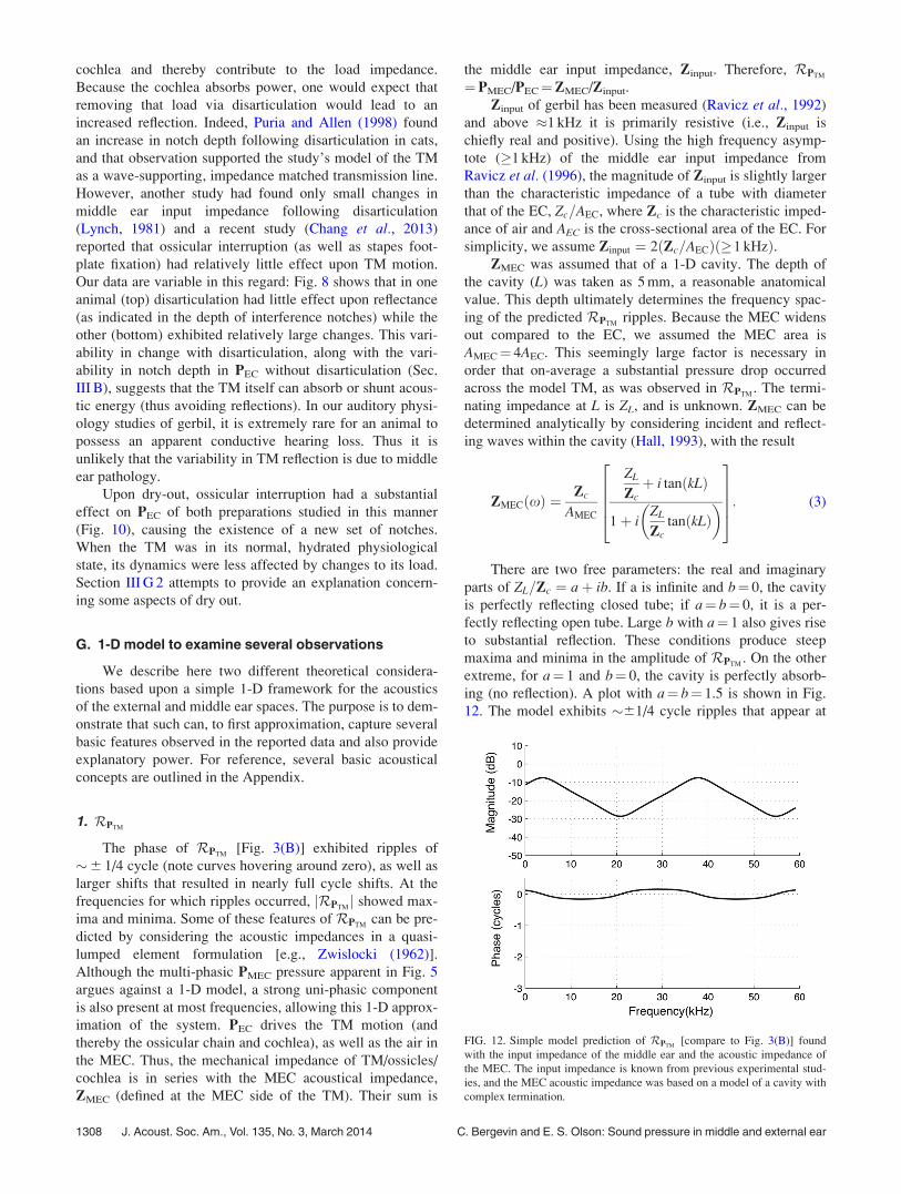
simplicity, we assume Zinput ¼ 2ðZc=AECÞð1 kHzÞ.ZMEC was assumed that of a 1-D cavity. The depth of

the cavity (L) was taken as 5 mm, a reasonable anatomical

value. This depth ultimately determines the frequency spac-

ing of the predicted RPTMripples. Because the MEC widens

out compared to the EC, we assumed the MEC area is

AMEC¼ 4AEC. This seemingly large factor is necessary in

order that on-average a substantial pressure drop occurred

across the model TM, as was observed in RPTM. The termi-

nating impedance at L is ZL, and is unknown. ZMEC can be

determined analytically by considering incident and reflect-

ing waves within the cavity (Hall, 1993), with the result

ZMECðxÞ ¼Zc

AMEC

ZL

Zcþ i tanðkLÞ

1þ iZL

ZctanðkLÞ

� �26664

37775: (3)

There are two free parameters: the real and imaginary

parts of ZL=Zc ¼ aþ ib. If a is infinite and b¼ 0, the cavity

is perfectly reflecting closed tube; if a¼ b¼ 0, it is a per-

fectly reflecting open tube. Large b with a¼ 1 also gives rise

to substantial reflection. These conditions produce steep

maxima and minima in the amplitude of RPTM. On the other

extreme, for a¼ 1 and b¼ 0, the cavity is perfectly absorb-

ing (no reflection). A plot with a¼ b¼ 1.5 is shown in Fig.

12. The model exhibits �61/4 cycle ripples that appear at

FIG. 12. Simple model prediction of RPTM[compare to Fig. 3(B)] found

with the input impedance of the middle ear and the acoustic impedance of

the MEC. The input impedance is known from previous experimental stud-

ies, and the MEC acoustic impedance was based on a model of a cavity with

complex termination.


frequencies for which the amplitude ratio has maxima and

minima. The size and spacing of the maxima and minima are

similar to what was observed. Thus, several aspects of the

data can emerge from a simple 1-D model for the MEC

impedance.

The analysis of Fig. 12 was based on reflections from

the back wall of the MEC cavity and these reflections also

would produce spatial pressure variations within the MEC.

The standing wave ratio (the ratio of the maximum to the

minimum pressure at different locations, and one frequency)

is set by the terminating impedance. With the a and b param-

eter values used here, the predicted standing wave ratio

within the MEC was 3.4, or 11 dB. These predicted spatial

variations are not as large as those measured in the MEC

(Fig. 6), where the standing wave ratio could be greater than

30 dB. Although useful for some basic understanding, the 1-

D model is far from a complete description.

2. Dry out and disarticulation

We expand our analysis from Sec. I to examine the EC

pressure in more detail. Similar to ZMEC above, we treat the

canal simply as a 1-D tube with variable terminating imped-

ance Z0. First, by assuming the TM acts as a stiffness only

[i.e., Z0(x)¼�is/x], the spatial location of a notch will

occur at

xðx; sÞ ¼ c

2xp� arctan

2sxx2 � s2

� �� : (4)

This expression indicates that the position of a pressure null

can vary with the stiffness of the terminating load. In the

limit of very high stiffness (i.e., a rigid boundary), the

quantity

2sxx2 � s2

� �! 0:

Considering principal values only, we obtain

x ¼ c

4f; (5)

where f¼x/(2p). This is just the characteristic quarterwavelength known for rigid tubes.

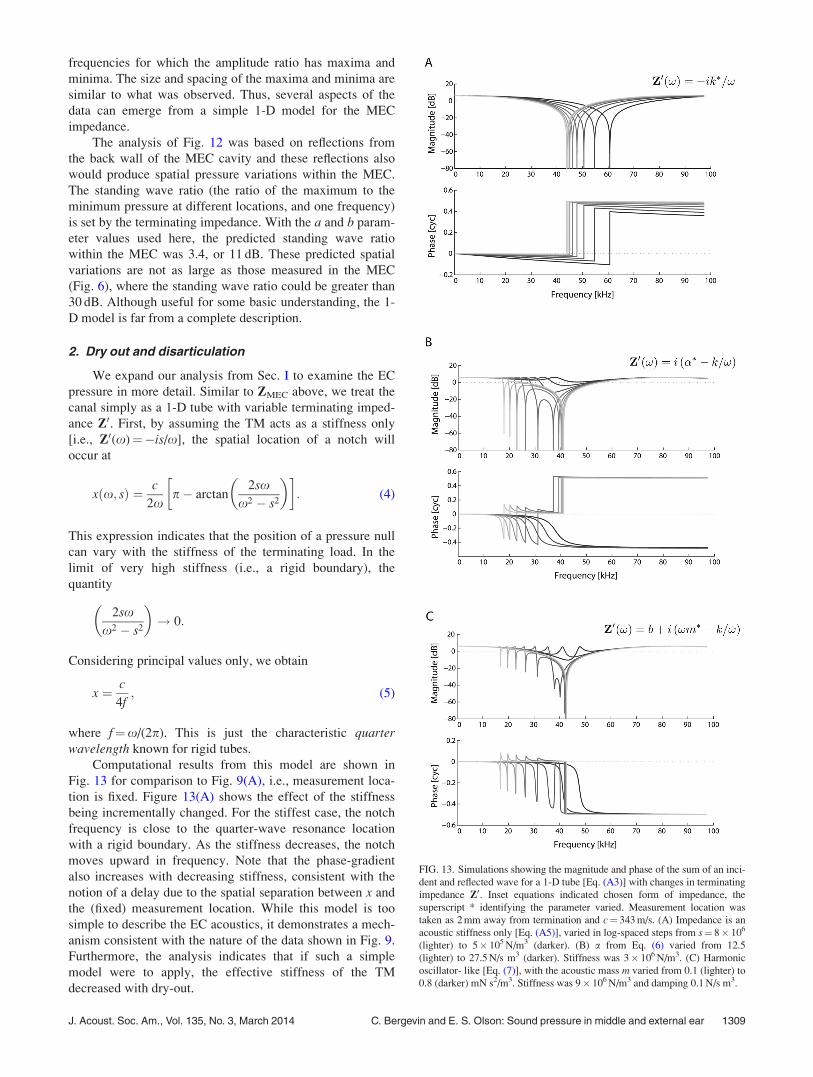
Computational results from this model are shown in

Fig. 13 for comparison to Fig. 9(A), i.e., measurement loca-

tion is fixed. Figure 13(A) shows the effect of the stiffness

being incrementally changed. For the stiffest case, the notch

frequency is close to the quarter-wave resonance location

with a rigid boundary. As the stiffness decreases, the notch

moves upward in frequency. Note that the phase-gradient

also increases with decreasing stiffness, consistent with the

notion of a delay due to the spatial separation between x and

the (fixed) measurement location. While this model is too

simple to describe the EC acoustics, it demonstrates a mech-

anism consistent with the nature of the data shown in Fig. 9.

Furthermore, the analysis indicates that if such a simple

model were to apply, the effective stiffness of the TM

decreased with dry-out.

FIG. 13. Simulations showing the magnitude and phase of the sum of an inci-

dent and reflected wave for a 1-D tube [Eq. (A3)] with changes in terminating

impedance Z0. Inset equations indicated chosen form of impedance, the

superscript * identifying the parameter varied. Measurement location was

taken as 2 mm away from termination and c¼ 343 m/s. (A) Impedance is an

acoustic stiffness only [Eq. (A5)], varied in log-spaced steps from s¼ 8� 106

(lighter) to 5� 105 N/m3 (darker). (B) a from Eq. (6) varied from 12.5

(lighter) to 27.5 N/s m3 (darker). Stiffness was 3� 106 N/m3. (C) Harmonic

oscillator- like [Eq. (7)], with the acoustic mass m varied from 0.1 (lighter) to

0.8 (darker) mN s2/m3. Stiffness was 9� 106 N/m3 and damping 0.1 N/s m3.


We can modify the terminating impedance in other

ways to describe more complex conditions. Heuristically,

consider

Z0ðxÞ ¼ iða� s=xÞ; (6)

where a 2 R. The extra reactive term due to a is neither a

stiffness or mass (due to lack of dependence upon x).8 Such

an expression for the impedance leads to the existence of a

second notch [Fig. 13(B)], noting that both notches can dis-

appear altogether depending upon the relative values of aand s. Such may help explain observations of changes due to

disarticulation in the dried out state (Fig. 10), where an addi-

tional notch manifests. We can also consider the terminating

impedance as that of a harmonic oscillator (Rabbitt, 1990),

given by

Z0ðxÞ ¼ bþ iðmx� k=xÞ: (7)

As shown in Fig. 13(C), varying the mass while holding the

damping and stiffness constant causes a second notch to

manifest when the resonant frequency is near (but below)

the quarter wave resonance frequency. While these 1-D

models are too simple to fully explain the observed data,

they are useful to help understand the basis for the changes

in PEC upon dry-out and disarticulation.

V. SUMMARY

Our study has experimentally examined the acoustics

throughout the gerbil (residual) external and middle ear

spaces, focusing chiefly on higher frequencies (1–60 kHz).

Returning to the questions initially posed at the outset, we

have found that:

(1) There is a significant pressure drop across the TM at

most frequencies. Thus, the external-stimulus-induced

EC-side sound pressure at the TM can be considered

the drive to the TM (and ultimately the cochlea).

(2) On the EC-side, variations in the pressure along the TM

surface are relatively small, indicative of a uniform

driving pressure. However on the MEC-side, these sur-

face variations are significant. This is likely because the

multi-phasic TM motion is able to more significantly

affect the (relatively smaller) pressure on the MEC

side.

(3) Significant spatial variations in MEC pressure exist, pre-

sumably due to interference stemming from reflections

throughout the bony cavity. In some frequency regions

these reflections appear to be large enough to shape the

pressure difference that drives TM motion.

(4) The physiological state of the TM has a significant effect

upon external and middle ear acoustics. In a dried out

state, changes in ossicular coupling are accentuated,

whereas in vivo changes due to disarticulation are less

drastic. Opening of parsF has a relatively small effect

upon the acoustics about the TM, despite a direct path

for sound energy into the MEC. However, opening

of parsT caused substantial spatial variations in EC

acoustics.

We employed a simple 1-D modeling framework to inter-

pret some of the findings. Beyond that, these experimental

results should prove useful to more detailed theoretical mod-

els for the mammalian external/middle ear [e.g., Funnell et al.(1987); Rabbitt (1990); Ravicz et al. (1992); Puria and Allen

(1998); Gan et al. (2006); Fay et al. (2006); Parent and Allen

(2007); Goll and Dalhoff (2011)] to better elucidate the

dynamic role of the TM.

ACKNOWLEDGMENTS

Technical assistance from Wei Dong, Michael Ravicz,

Chris Shera, and Polina Varrava is gratefully acknowledged.

Work was supported by NIH NIDCD R01-DC003130 (EO)

and an NSERC Discovery Grant (CB).

APPENDIX

We describe here some basic acoustical concepts rele-

vant for Sec. IV G. Consider a 1-D tube whose longitudinal

axis is described by the spatial dimension x and is filled with

some medium(s) whose specific acoustic impedance is

Z¼ qc where q is the medium’s density [kg/m3] and c the

speed of sound in the medium. The incident pressure wave

(pi) propagates in the þx direction, the “reflected” wave (pr)

along �x. Each wave also has an associated particle velocity

(vi and vr). All bold quantities can be described by their re-

spective Fourier coefficients,

pðx;x; tÞ ¼ pi þ pr ¼ PiðxÞeixðt�x=cÞþPrðxÞeixðtþx=cÞ:

(A1)

Consider two adjacent mediums inside the tube, each

with their own characteristic acoustic impedances (for exam-

ple, Z1¼q1c1 and Z2¼q2c2), their interface at x¼ 0 being

the discontinuous boundary condition. The impedances

away from the boundary are given by

Pi

Vi¼ Z1

Pr

Vr¼ �Z1

Pt

Vt¼ Z2;

where the subscript t indicates the transmitted component. The

reflectance is defined as R � Pr=Pi and can be expressed as

RðxÞ¼Z0 � 1

Z0 þ 1; (A2)

where Z0 � Z2=Z1. From Eq. (A2), the reflectance explicitly

depends upon the (normalized) impedance (Z0) the incident

wave is subject to at the interface. That is, the terminating

load directly affects the properties of the reflected wave and

thereby interference between Pi and Pr. Such is apparent if

we rewite Eq. (A1) as

pðx;xÞ � PiðxÞ½e�ixx=cþRðxÞeixx=c�: (A3)

Consider a maximal null, that is, a spatial location

where the two waves fully cancel one another out due to de-

structive interference. From Eq. (A3), two conditions must

be met for such a null


je�ixx=cj ¼ jRðxÞeixx=cj;

�xx=c ¼ xx=cþ hþ p;

where h � /R ¼ /½ðZ0 � 1Þ=ðZ0þ1Þ�. The first equation

simply indicates that jRj ¼ 1. The second equation indicates

that the phase difference must be a half cycle. Rearranging,

we have

x ¼ c

2xð7p� hÞ (A4)

(the 7 comes from the phase wrapping ambiguity). Even in

the case of a null where the two waves do not fully cancel

out (i.e., jRj < 1), Eq. (A4) still needs to be satisfied.

Consider the case where the terminating load can be

described simply by a stiffness

Z0ðxÞ ¼ �is=x; (A5)

where s is the stiffness coefficient. Then from Eq. (A2), we

have

RsðxÞ ¼isþ xis� x

; (A6)

where the subscript indicates a stiffness only. Solving for the

phase leads to

/Rs ¼ h ¼ tan�1 2sxx2 � s2

� �:

Plugging this back into Eq. (A4) (and ignoring the phase

wrapping ambiguity) leads to Eq. (4).

1We use middle ear cavity (MEC) in the current report and consider the

term bulla space to be synonymous. Physically the MEC comprises all

mechanically relevant structures between the tympanic membrane and sta-

pes footplate, including the ossicles and coupling to other cavities via the

Eustachian tube.2There is potential for ambiguity in this chosen coordinate system. For

example, two different locations on the TM, each with a unique (x, y) pair,

could meet at the same point when projected out along z. Thus, this system

is not suitable for a rigorous theoretical framework, but is ultimately suffi-

cient to describe the measurements and analysis here.3Considering a simple elastic circular membrane, uni-phasic motion would

correspond to the (m, n)¼ (0, 1) mode, where m and n represent radially

constant and radially symmetric nodes respectively. Multi-phasic modes

exist when either n> 0 or m> 1.4Because the sensors typically remained in air and rarely had direct contact

with hard surfaces, their stability was good. Most sensors lasted at least

several experiments and their sensitivity varied less than several dB across

that span.5This required use of extracted temporal bones, which dried significantly

faster than when left embedded in the head. It was also harder to visually

verify spatial placement of the sensor for a given measurement.6Given the small working distances and fragility of the sensor, it was diffi-

cult to seal the bullar hole while the sensor was inside.7For all measurements reported here for positions close to the TM (i.e.,

jzj � 40 lm), the sensor was not touching the TM, based upon visual veri-

fication both before and after a given experimental run. However, during

several experiments it was observed that the sensor had become stuck to

the TM at some point during a given run. This was more common during

in vivo experiments when more moisture was present. Interestingly, there

was little difference in the measured pressure between runs where the sen-

sor was or was not touching the TM. Such an observation indicates that

the measured pressure was not affected either by the sensor locally chang-

ing the TM motion nor the sensor itself being moved by the TM.8Such a term does not have a direct physical analog: since the impulse

response is a real function, the reactive term (i.e., imaginary part of the

Fourier transform) must be an odd function of x, which is not generally

the case for Eq. (6).

Chang, E. W., Cheng, J. T., R€o€osli, C., Kobler, J. B., Rosowski, J. J., and

Yun, S. H. (2013). “Simultaneous 3D imaging of sound-induced motions

of the tympanic membrane and middle ear ossicles,” Hear. Res. 304,

49–56.

Cheng, J. T., Hamade, M., Merchant, S. N., Rosowski, J. J., Harrington, E.,

and Furlong, C. (2013). “Wave motion on the surface of the human tym-

panic membrane: Holographic measurement and modeling analysis,”

J. Acoust. Soc. Am. 133, 918–937.

Dalhoff, E., Turcanu, D., and Gummer, A. W. (2011). “Forward and reverse

transfer functions of the middle ear based on pressure and velocity

DPOAEs with implications for differential hearing diagnosis,” Hear. Res.

280, 86–99.

Decraemer, W. F., Khanna, S. M., and Funnell, W. R. (1989).

“Interferometric measurement of the amplitude and phase of tympanic

membrane vibrations in cat,” Hear. Res. 38, 1–17.

de La Rochefoucauld, O., Decraemer, W. F., Khanna, S. M., and Olson, E.

S. (2008). “Simultaneous measurements of ossicular velocity and intraco-

chlear pressure leading to the cochlear input impedance in gerbil,”

J. Assoc. Res. Otolaryngol. 9, 161–177.

de La Rochefoucauld, O., Kachroo, P., and Olson, E. S. (2010). “Ossicular

motion related to middle ear transmission delay in gerbil,” Hear. Res. 270,

158–172.

de La Rochefoucauld, O., and Olson, E. S. (2010). “A sum of simple and

complex motions on the eardrum and manubrium in gerbil,” Hear. Res.

263, 9–15.

Dong, W., Decraemer, W. F., and Olson, E. S. (2012). “Reverse

Transmission along the Ossicular Chain in Gerbil,” J. Assoc. Res.

Otolaryngol. 13, 447–459.

Dong, W., and Olson, E. S. (2006). “Middle ear forward and reverse trans-

mission in gerbil,” J. Neurophysiol. 95, 2951–2961.

Fay, J. P., Puria, S., and Steele, C. R. (2006). “The discordant eardrum,”

Proc. Natl. Acad. Sci. U.S.A. 103, 19743–19748.

Feeney, M. P., and Keefe, D. H. (1999). “Acoustic reflex detection using

wide-band acoustic reflectance, admittance, and power measurements,”

J. Speech Lang. Hear. Res. 42, 1029–1041.

Funnell, W. R. J., Decraemer, W. F., and Khanna, S. M. (1987). “On the

damped frequency response of a finite-element model of the cat eardrum,”

J. Acoust. Soc. Am. 81, 1851–1859.

Furlong, C., Rosowski, J., Hulli, N., and Ravicz, M. (2009). “Preliminary

analyses of tympanic membrane motion from holographic measurements,”

Strain 45, 301–309.

Gan, R., Feng, B., and Sun, Q. (2004). “Three-dimensional finite element

modeling of human ear for sound transmission–springer,” Annals Biomed.

Eng. 32, 847–859.

Gan, R. Z., Sun, Q., Feng, B., and Wood, M. W. (2006). “Acoustic-struc-

tural coupled finite element analysis for sound transmission in human ear-

pressure distributions,” Med. Eng. Phys. 28, 395–404.

Goll, E., and Dalhoff, E. (2011). “Modeling the eardrum as a string with dis-

tributed force,” J. Acoust. Soc. Am. 130, 1452–1462.

Hall, D. E. (1993). Basic Acoustics (Krieger, Malabar, FL), pp. 243–249.

Keefe, D. H., Fitzpatrick, D., Liu, Y.-W., Sanford, C. A., and Gorga, M. P.

(2010). “Wideband acoustic-reflex test in a test battery to predict middle-

ear dysfunction,” Hear. Res. 263, 52–65.

Keefe, D. H., Ling, R., and Bulen, J. C. (1992). “Method to measure acous-

tic impedance and reflection coefficient,” J. Acoust. Soc. Am. 91,

470–485.

Khanna, S., and Tonndorf, J. (1972). “Tympanic membrane vibrations in

cats studied by time-averaged holography,” J. Acoust. Soc. Am. 51,

1904–1920.

Leonard, R. W. (1964). “Probe-Tube Microphones,” J. Acoust. Soc. Am. 36,

1867–1871.

Lynch, T. J. (1981). “Signal processing by the cat middle ear: Admittance

and transmission, measurements and models,” Ph.D. thesis, Massachusetts

Institute of Technology.

Lynch, T. J., Peake, W. T., and Rosowski, J. J. (1994). “Measurements of

the acoustic input impedance of cat ears: 10 Hz to 20 kHz,” J. Acoust.

Soc. Am. 96, 2184–2209.


Maftoon, N., Funnell, W. R. J., Daniel, S. J., and Decraemer, W. F. (2013).

“Experimental study of vibrations of gerbil tympanic membrane with

closed middle ear cavity,” J. Assoc. Res. Otolaryngol. 14, 467–481.

Manley, G. (1972). “The middle ear of the Tokay Gecko,” J. Comp. Physiol.

A 81, 239–250.

Nakajima, H. H., Ravicz, M. E., Merchant, S. N., Peake, W. T., and J

Rosowski, J. (2005). “Experimental ossicular fixations and the middle

ear’s response to sound: Evidence for a flexible ossicular chain,” Hear.

Res. 204, 60–77.

Olson, E. (1998). “Observing middle and inner ear mechanics with novel

intracochlear pressure sensors,” J. Acoust. Soc. Am. 103, 3445–3463.

Parent, P., and Allen, J. (2007). “Wave model of the cat tympanic mem-

brane,” J. Acoust. Soc. Am. 122, 918–931.

Pinder, A. C., and Palmer, A. R. (1983). “Mechanical properties of the frog

ear: vibration measurements under free- and closed-field acoustic con-

ditions,” Proc. R. Soc. Sec. B 219, 371–396.

Puria, S. (2003). “Measurements of human middle ear forward and reverse

acoustics: Implications for otoacoustic emissions,” J. Acoust. Soc. Am.

113, 2773–2789.

Puria, S., and Allen, J. B. (1998). “Measurements and model of the cat mid-

dle ear: evidence of tympanic membrane acoustic delay,” J. Acoust. Soc.

Am. 104, 3463–3481.

Rabbitt, R. (1990). “A hierarchy of examples illustrating the acoustic cou-

pling of the eardrum,” J. Acoust. Soc. Am. 87, 2566–2582.

Ravicz, M., Olson, E., and Rosowski, J. (2007). “Sound pressure distribution

and power flow within the gerbil ear canal from 100 Hz to 80 kHz,”

J. Acoust. Soc. Am. 122, 2154–2173.

Ravicz, M., Rosowski, J., and Voigt, H. (1992). “Sound-power collection by

the auditory periphery of the Mongolian gerbil Meriones unguiculatus. I:

Middle ear input impedance,” J. Acoust. Soc. Am. 92, 157–177.

Ravicz, M. Rosowski, J., and Voigt, H. (1996). “Sound-power collection by

the auditory periphery of the Mongolian gerbil Meriones unguiculatus. II.

External-ear radiation impedance and power collection,” J. Acoust. Soc.

Am. 99, 3044–3063.

Rosowski, J. J., Dobrev, I., Khaleghi, M., Lu, W., Cheng, J. T., Harrington,

E., and Furlong, C. (2013). “Measurements of three-dimensional shape

and sound-induced motion of the chinchilla tympanic membrane,” Hear.

Res. 301, 44–52.

Rosowski, J. J., Ravicz, M. E., Teoh, S. W., and Flandermeyer, D. (1999).

“Measurements of middle-ear function in the Mongolian gerbil, a special-

ized mammalian ear,” Audiol. Neurotol. 4, 129–136.

Rosowski, J. J., and Saunders, J. C. (1980). “Sound transmission through the

avian interaural pathways,” J. Comp. Physiol. A 136, 183–190.

Russell, D. A. (2010). “Basketballs as spherical acoustic cavities,” Am. J.

Phys. 78, 549–554.

Schmiedt, R. A., and Zwislocki, J. J. (1977). “Comparison of sound trans-

mission and cochlear microphonic characteristics in Mongolian gerbil and

guinea pig,” J. Acoust. Soc. Am. 61, 133–149.

Shera, C. A., and Zweig, G. (1992). “Middle-ear phenomenology: the view

from the three windows,” J. Acoust. Soc. Am. 92, 1356–1370.

Sokolich, W. G. (1977). “Improved acoustic system for auditory research,”

J. Acoust. Soc. Am. 62, S12.

Stinson, M. R. (1985). “Spatial variation of phase in ducts and the measure-

ment of acoustic energy reflection coefficients,” J. Acoust. Soc. Am. 77,

386–393.

Stinson, M. R., and Khanna, S. M. (1989). “Sound propagation in the ear

canal and coupling to the eardrum, with measurements on model systems,”

J. Acoust. Soc. Am. 85, 2481–2491.

Stinson, M. R. Shaw, E. A., and Lawton, B. W. (1982). “Estimation of

acoustical energy reflectance at the eardrum from measurements of pres-

sure distribution in the human ear canal,” J. Acoust. Soc. Am. 72,

766–773.

Teoh, S., Flandermeyer, D., and Rosowski, J. (1997). “Effects of pars flac-

cida on sound conduction in ears of Mongolian gerbil: acoustic and ana-

tomical measurements,” Hear. Res. 106, 39–65.

van Dijk, P., Mason, M. J., Schoffelen, R. L. M., Narins, P. M., and

Meenderink, S. W. F. (2011). “Mechanics of the frog ear,” Hear. Res. 273,

46–58.

Voss, S., and Shera, C. (2004). “Simultaneous measurement of middle-ear

input impedance and forward/reverse transmission in cat,” J. Acoust. Soc.

Am. 116, 2187–2198.

Voss, S. E., Rosowski, J. J., Merchant, S. N., and Peake, W. T. (2001).

“Middle-ear function with tympanic-membrane perforations. I.

Measurements and mechanisms,” J. Acoust. Soc. Am. 110, 1432–1444.

Zwislocki, J. (1962). “Analysis of the middle ear function. Part I: Input

impedance,” J. Acoust. Soc. Am. 34, 1514–1523.


External and middle ear sound pressure distribution and ... · External and middle ear sound...

Documents

Transcript of External and middle ear sound pressure distribution and ... · External and middle ear sound...