EXTENSION OF THE TRANSMISSION LINE THEORY APPLICATION WITH...

Progress In Electromagnetics Research M, Vol. 32, 257–270, 2013

EXTENSION OF THE TRANSMISSION LINE THEORYAPPLICATION WITH MODIFIED ENHANCED PER-UNIT-LENGTH PARAMETERS

Sofiane Chabane1, *, Philippe Besnier1, and Marco Klingler2

1IETR, Institute of Electronics and Telecommunications of Rennes,CNRS UMR 6164, INSA of Rennes, 20 Av. des Buttes de Coesmes,CS 14315, Rennes Cedex 35043, France2PSA Peugeot-Citroen, Centre Technique de Velizy, 2 route de Gisy,78943 Velizy-Villacoublay Cedex, France

Abstract—This paper introduces a modified enhanced transmission-line theory to account for higher-order modes while using a standardtransmission line equation solver or equivalently a Baum, Liu andTesche (BLT) equation solver. The complex per-unit-length parametersas defined by Nitsch et al. are first cast into an appropriate per-unit-length resistance, inductance, capacitance and conductance (RLCG)form. Besides, these per-unit-length parameters are modified toaccount for radiation losses with reasonable approximations. Thismodification is introduced by an additional per-unit-length resistance.The reason and explanations for this parameter are provided. Resultsobtained with this new formalism are comparable to those obtainedusing an electromagnetic full-wave solver, thus extending the capabilityof conventional transmission line solvers.

1. INTRODUCTION

Complex systems such as automobiles or other vehicles have to meetelectromagnetic compatibility (EMC) requirements. Design engineersneed to predict the performances of their products in the early stageof their development. EMC simulation tools should be able to helpdevelopers to analyze the EMC performances of the vehicle and itselectrical and electronic architecture.

Received 23 July 2013, Accepted 28 August 2013, Scheduled 1 September 2013* Corresponding author: Sofiane Chabane ([email protected]).

258 Chabane, Besnier, and Klingler

The most vulnerable point of a vehicle is its equipment,since faults caused to the equipment modules may lead to varioustypes of malfunctions. These faults may be the consequence ofthe induced currents and voltages on the wires of the harnesses.The electromagnetic interference calculations at the end of harnessnetworks are still a challenge for many equipment modules or systems.Topology of harnesses and the important number of individual wiresis one obvious reason for this.

Hopefully, given the relative proximity of wires to the surroundinglarge metallic or conducting structures, the transmission line theory(TLT) is applied in most cases. It thus reduces the complexity andthe cost of calculations. Using the field to transmission line (TL)coupling formalism such as Agrawal’s model [1], it is possible to splitcalculations into two decoupled problems. First, the field calculationalong the routes of the harnesses in absence of the wiring is performedby the means of a 3D Maxwell’s equation solver. Then, a multi-conductor transmission line solver is used to calculate currents andvoltages induced on the wires, using the field values calculated in thefirst step.

However, TLT is limited by some assumptions that are not alwaysunder control and cannot always be used. Indeed, the classicalTLT equations can easily be derived from Maxwell’s equations afterapproximating the Green’s function relating the sources (incidentelectromagnetic field) to the reaction of the wire (induced currentsand voltages) [2]. The main assumption is that the distance betweenthe TL and its return path should be much smaller than the minimumconsidered wavelength of the current flowing in it. As a consequenceof this simplification, the result of the Green’s function integral alongthe TL contains no imaginary part, i.e., the radiation resistance isaltogether neglected and the wave is considered totally guided alongthe TL.

Nevertheless, there are some situations for which this approxima-tion may not stand. Obviously, it’s difficult to establish a definite limitof the separation distance that must not be exceeded unless one im-poses an arbitrary criterion. Moreover, this approximation may yieldto inaccurate current estimations at the resonance frequencies, since inthis case the radiation resistance may play an important role.

For these reasons, extending the ability of the TLT to handlehigher order modes while keeping the simplicity of its formalism wouldbe a significant improvement.

Numerous advanced studies have met some success in thisdirection. Some new models have been directly derived from Maxwell’sequations without the height limitation. However, most of these

Progress In Electromagnetics Research M, Vol. 32, 2013 259

models are based on iterative time- and memory-consuming solutions,and are rather suitable either for mono conductor situations [3] or forshort conductors such as the interconnects [4].

The more general and rigorous formalism is the one known as thetransmission line super theory [5]. This theory presents a rigorousderivation of Maxwell’s equations for non-uniform transmission linesinto a set of coupled equations which resembles the telegrapher’sequations. The per-unit-length (p.u.l.) parameters, which are position-and frequency-dependent, are calculated through a rather complexiterative procedure. Besides, the computation of the solution of theseequations remains cumbersome and needs an entire new softwaredevelopment.

The enhanced transmission line p.u.l. parameters defined in [6]allow taking into account higher-order modes for uniform transmissionlines using a rigorous derivation of the integral of the Green’s function.However, these enhanced p.u.l. parameters cannot directly be used ina TLT solver (like the Baum, Liu and Tesche (BLT) equation-basedsolver [7, 8]) and therefore require an entire new software development.

The purpose of this paper is, on the one hand, to derive aproper representation of these parameters easy to embed in a classicalTL solver or in its BLT form solver and, on the other hand, toshow how the energy related to the radiation is dissipated. Indeed,putting the complex p.u.l. parameters defined in [6] under a resistance,inductance, capacitance, conductance (RLCG) form leads only to thedecomposition of the modes in terms of TEM modes supported bythe real part of the characteristic impedance, and radiating modes (orantenna mode) supported by the imaginary part of the characteristicimpedance. Therefore, in this paper, we will also present a modifiedversion of these enhanced parameters that will converge to the solutionof the differential currents at the ends of the TL. This solutionallows calculating these currents using a classical BLT solver with agood approximation, even at critical resonant frequencies or when theconditions of application of the classical TLT are not fulfilled. In thispaper, we present and validate this method for a single wire above aperfect ground plane.

2. ENHANCED TRANSMISSION-LINE THEORY

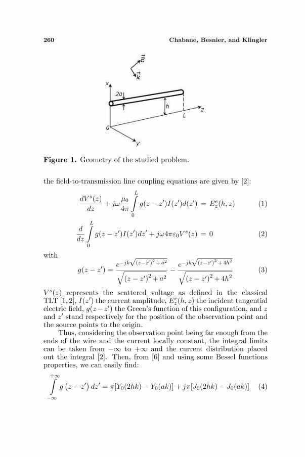
Let us consider a lossless TL above a perfectly conducting (PEC)ground plane in presence of an external electromagnetic field as shownin Fig. 1.

From Maxwell’s equations, and using the thin wire approximation,


Figure 1. Geometry of the studied problem.

the field-to-transmission line coupling equations are given by [2]:

dV s(z)dz

+ jωµ0

4π

L∫

0

g(z − z′)I(z′)d(z′) = Eez(h, z) (1)

d

dz

L∫

0

g(z − z′)I(z′)dz′ + jω4πε0Vs(z) = 0 (2)

with

g(z − z′) =e−jk

√(z−z′)2 + a2

√(z − z′)2 + a2

− e−jk√

(z−z′)2 +4h2

√(z − z′)2 +4h2

(3)

V s(z) represents the scattered voltage as defined in the classicalTLT [1, 2], I(z′) the current amplitude, Ee

z(h, z) the incident tangentialelectric field, g(z−z′) the Green’s function of this configuration, and zand z′ stand respectively for the position of the observation point andthe source points to the origin.

Thus, considering the observation point being far enough from theends of the wire and the current locally constant, the integral limitscan be taken from −∞ to +∞ and the current distribution placedout the integral [2]. Then, from [6] and using some Bessel functionsproperties, we can easily find:

+∞∫

−∞g

(z − z′

)dz′ = π[Y0(2hk)− Y0(ak)] + jπ[J0(2hk)− J0(ak)] (4)


Here J0 and Y0 are, respectively, the 0-order Bessel functions of firstand second kind.

Now, using the expansion form of Y0 as given in [9]:

Y0(z) =2π

[ln

z

2+ γ

]J0(z)− 2

π

∞∑

k=1

(−1)k

(z2

)2k

(k!)2

(k∑

m=1

1m

)(5)

and after some rearrangements the above integral (4) can be rewrittenas:

+∞∫

−∞g

(z − z′

)dz′

= 2 ln(

2h

a

)+2

[ln(hk)+γ][J0(2hk)−1]−

[ln

(ak

2

)+γ

][J0(ak)−1]

−2

[ ∞∑

k=1

(−1)k (hk)2k

(k!)2

(k∑

m=1

1m

)]−

[ ∞∑

k=1

(−1)k

(ak2

)2k

(k!)2

(k∑

m=1

1m

)]

+jπ[J0(2hk)− J0(ak)] (6)

The classical approximation for this integral consists in assuming thatall terms are negligible with respect to the first one on the right-handside of (6). In the following these terms are considered as a correctionfactor.

Hereafter, we express the real part of this correction factor as:

R(CF ) = 2[ln(hk) + γ][J0(2hk)− 1]−

[ln

(ak

2

)+γ

][J0(ak)−1]

−2

[ ∞∑

k=1

(−1)k (hk)2k

(k!)2

(k∑

m=1

1m

)]

−[ ∞∑

k=1

(−1)k (ak2 )2k

(k!)2

(k∑

m=1

1m

)](7)

and the imaginary part as:

= (CF ) = π [J0 (2hk)− J0 (ak)] (8)

Using these definitions and substituting them in (1) and (2), we get:

dV s(z)dz

+ I(z)(jωLHF + RHF

)= Ee

z(h, z) (9)

dI(z)dz

+ V s(z)(jωCHF + GHF

)= 0 (10)


where the explicit forms of these p.u.l. parameters are given by:

LHF = L′0 +

µ0

4π< (CF ) (11)

RHF = −ωµ0

4π= (CF ) (12)

CHF =C′0

[2 ln

(2ha

)+ < (CF )

]4 ln2( 2h

a )+4<(CF ) ln( 2ha )+<(CF )2+=(CF )2

2 ln( 2ha )

(13)

GHF =ωC

′0= (CF )

4 ln2( 2ha )+4<(CF ) ln( 2h

a )+<(CF )2+=(CF )2

2 ln( 2ha )

(14)

and where the classical p.u.l. parameters are given by:

L′0 =

µ0

2πln

(2h

a

)(15)

andC′0 =

2πε0

ln(

2ha

) (16)

Note that (9) and (10) have exactly the same form as the classicalones. Hence, to solve this system all the known methods of resolutionin the classical case can be used here. In our case, we use the BLTformulation of the TL equations.

Besides, the new enhanced p.u.l. parameters are now frequency-dependent and are not limited to the quasi-static approximation butreduced to the classical ones where the classical TLT assumptions arefulfilled.

The resistance and the (negative) conductance parameters accountfor higher-order modes whereas the frequency-dependent inductanceand capacitance can differ significantly from the classical ones,especially when the quasi-static approximation is no longer valid.

Since the p.u.l. parameters are enhanced and become frequency-dependent, we can expect that the characteristic impedance is alsofrequency-dependent.

From (4), (1) and (2), we find that the enhanced p.u.l. impedanceis given by:

z = jωµ0

4ππ [Y0 (2hk)− Y0 (ak)] + jπ [J0 (2hk)− J0 (ak)] (17)

The enhanced per-unit-length admittance is written as:

y = jω4πε0

π [Y0 (2hk)− Y0 (ak)] + jπ [J0 (2hk)− J0 (ak)](18)


Using the classical definition of the characteristic impedance as thesquare root of the ratio between the impedance and the admittance:

Zc =√

z

y(19)

It can easily be proven that the enhanced characteristic impedance iscomplex and is given by:

Zc =14π

√µ0

ε0π [Y0 (2hk)− Y0 (ak)] + jπ [J0 (2hk)− J0 (ak)] (20)

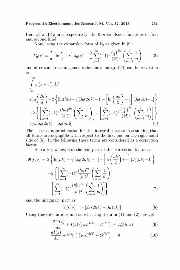
Thus, the characteristic impedance, even for a lossless transmis-sion line, becomes complex and frequency-dependent (Fig. 2).

Figure 2. Comparison between the classical and enhancedcharacteristic impedance for a lossless TL above a PEC ground, height= 0.3m, radius = 1mm.

Now, we investigate the effect of the enhanced p.u.l. parameterson the propagation constant.

The propagation constant, in its general form is given by:

γ = α + jβ (21)

where α and β are, respectively, the attenuation and phase constants.The propagation constant is calculated through:

γ2 = ZY =(RHF + jLHF ω

) (GHF + jCHF ω

)(22)


Replacing ZY in (22) by (17) and (18), we get:

γ2 = −ω2µ0ε0 (23)

Since the result of the product is a pure negative real value, thepropagation constant is a pure imaginary term. This means that theuse of these new p.u.l. parameters will not lead to energy dissipation.In other words, the energy is still stored in the TL. Nevertheless, theseenhanced parameters allow to split the energy propagating on the TLinto TEM and radiated modes as shown below.

Indeed, (19) can also be written as:

Zc =

√RHF + jωLHF

GHF + jωCHF(24)

Considering that GHF ¿ ωCHF and using (8), (12) and (20) we caneasily get:

Zc =

√LHF

CHF− j

RHF

k(25)

The energy of the TEM mode is related to the real part of thecharacteristic impedance whereas the energy of the radiated mode isrelated to the imaginary part.

3. MODIFIED-ENHANCED P.U.L. PARAMETERS

As shown above, the enhanced p.u.l. parameters lead only to theseparation of the TEM mode and radiated mode on a TL. It meansthat the currents and voltages at the ends of the TL are not affectedand using these enhanced parameters does not provide more accurateresults. In order to dissipate the radiated energy, a possible method isto calculate appropriate reflection coefficients at the ends of the TL [2].We rather introduce a more convenient and new method that consistsin adding another p.u.l. resistance that will be related to the radiatedenergy.

This additional resistance R+ is inserted in series with RHF andLHF . The following developments present the theory related to thisadditional resistance in the case of a single wire above a ground plane.

Since an additional resistance R+ is introduced, the attenuationconstant α is non-null.

The wave attenuation factor for the square of the current (or ofthe voltage) over the length L of the TL can be written as:

A(L) = exp(−2αL) (26)


The power to be radiated can be associated with the ratio betweenthe imaginary part and the real part of the characteristic impedance,which is shown, in the following, to be equivalent to the definition ofthe quality factor Q of the TL.

From (25) this Q factor can easily be written as:

Qline =β

RHF

√LHF

CHF=

ωLHF

RHF(27)

When an additional resistance R+ is added to the p.u.l. parame-ters, (22) becomes:

γ2 =(RHF + R+ + jLHF ω

) (GHF + jCHF ω

)(28)

Considering the property RHF CHF = −LHF GHF and afterrearrangement, we get:

γ2 =(RHF + R+

)GHF − LHF CHF ω2 + jR+CHF ω (29)

In the following, we assume that∣∣(RHF + R+

)GHF

∣∣ ¿ LHF CHF ω2.Nevertheless, this assumption will be verified a posteriori. It must benoted that this condition is also equivalent to:

(RHF + R+

)RHF ¿ LHF 2

ω2 (30)

If this assumption is fulfilled, then γ2 can be approximated as:

γ2 ≈ −LHF CHF ω2 + jR+CHF ω (31)Since γ = α + jβ, it follows that:

2α2 ≈ LHF CHF ω2 − LHF CHF ω2

√(1− R2

+

LHF 2ω2

)(32)

The second term under the square root is verified to be much smallerthan one.

Then, a first order series expansion can be used to extract α2:

α2 =(R+)2 CHF

4LHF(33)

Using the definition of the attenuation factor in (26), (27) and (33),we find that the attenuation on the TL introduced by R+ is equal to:

A(0)−A(L) = 1− exp

(R+

√CHF

LHFL

)=

RHF

ωLHF(34)

In order to determine R+, this attenuation is identified with the inverseof the Q factor of the TL. Finally, we obtain:

R+ =1L

√LHF

CHFln

(1− RHF

ωLHF

)≈ RHF

βL(35)


As expected, the p.u.l. additional resistance is equivalent to theimaginary part of the characteristic impedance (25) distributed alongthe TL and is frequency-dependent (Fig. 3(a)). Besides, this additionalresistance does neither affect the phase constant nor the characteristic

(b)

(a)

Figure 3. Characteristics of the modified enhanced p.u.l. parametersfor a lossless TL above a PEC ground, height = 0.3m, radius = 1mm.(a) The additional correction resistance. (b) Characteristic impedanceand propagation constant.


impedance but only the attenuation constant (Fig. 3(b)). This is due tothe fact that it is relatively small compared to the p.u.l. resistance (35).

4. RESULTS

In order to validate this new model, some simulations have beencarried out. The p.u.l. parameters are calculated either using theirclassical form or using their modified enhanced version presentedpreviously. They are inserted in a BLT equation solver. Both resultsare compared to those obtained with an electromagnetic full-wavemethod of moments (MoM) solver (FEKO). The current in the loadis calculated as a function of the frequency of the excitation signal.Though the p.u.l. parameters, the associated characteristic impedanceand the propagation constant were calculated up to 2 GHz, in thefollowing the currents will be calculated only up to 500 MHz to keepthe clarity of the figures.

The configuration studied is presented in Fig. 4. It consists ina perfectly conducting and non-coated wire of 5 m length and 1 mmradius at 30 cm above a perfectly conducting ground plane. It is fedby a sinusoidal voltage source e of 1 V at one end and loaded with aresistance R of 1 Ω at the other end.

Figure 4. Setup of the studied circuit.

Figure 5 shows the current that flows in the resistance calculatedfrom three different methods. The black curve is calculated with theclassical TL equations. It highlights that the resonance levels are quitehigh and their amplitude does not follow a regular pattern since theydepend strongly on the frequency sampling points. Since no losses aretaken into account, the highest peak level is expected to be 0 dBA.The green curve shows the result of our modified enhanced versionof the TL solver. The level of the resonances follow a much moreregular evolution with frequency and calculations predict much lowerpeak levels as expected. For comparison, the calculation performedwith the MoM solver is presented in red.

Below roughly 300 MHz, results obtained with our model are ingood agreement with the full-wave solver. Beyond this frequency,the modified enhanced model does not provide results in agreement


Figure 5. Current amplitude as a function of the frequency at theend of the TL, using the modified enhanced p.u.l. parameters.

Figure 6. Current amplitude as a function of the frequency at the endof the TL, using the modified enhanced p.u.l. parameters and includingthe vertical wires.

with the MoM calculations. This can be explained by the effect ofthe vertical wires that are only modeled in the full-wave solver (forpractical reasons) and not in the TL approach. The effect of thesevertical wires can be approximately taken into account through theaddition of a p.u.l. resistance of these wires calculated from theradiation resistance of a monopole antenna [10, 11]. As expected(Fig. 6), this produces slightly better results (5 dB beyond 400MHz).


However, even with this correction, if we compare to the MoM resultsin Fig. 5, there are still some differences higher in frequency. This isdue to the monopole model used for the vertical wires and possiblyto the effect of the coupling between the horizontal and vertical wires.Nevertheless, in real cases, wires are not perfect conductors and as aconsequence, the amplitudes of the current induced in the loads areeven lower than predicted by the results in Figs. 5 and 6. Therefore,the proposed model leads to responses much more realistic than theclassical TLT model, and provides, in general, a better approximationespecially for the most critical first resonances.

5. CONCLUSIONS

In this paper, we have presented a modification to the enhancedper-unit-length (p.u.l.) parameters of a single transmission line (TL)which were first explicitly extracted from [6]. This modification wasnecessary since the enhanced parameters only enable to split the energypropagating on the TL into TEM and radiated modes. Thus, todissipate energy, an innovative solution has been demonstrated whichconsists in adding a supplementary p.u.l. resistance to the enhancedp.u.l. resistance and inductance. This additional p.u.l. resistancecorresponds approximately to the imaginary part of the characteristicimpedance of the TL. The results obtained are comparable to thoseobtained with a full-wave software even at resonant frequencies. Thisnew formalism is currently being generalized to take into account multi-conductor configurations and coated wires.

ACKNOWLEDGMENT

This work is sponsored by the French CNRS and PSA Peugeot-Citroen.

REFERENCES

1. Agrawal, A. K., H. J. Price, and S. H. Gurbaxani, “Transientresponse of a multiconductor transmission tine excited bya nonuniform electromagnetic field,” IEEE Transactions onElectromagnetic Compatibility, Vol. 22, No. 2, 119–129, May 1980.

2. Rachidi, S. V. and V. S. Tkachenko, Electromagnetic FieldInteraction with Transmission Lines. From Classical Theory toHF Radiation Effects, WIT Press, 2007.

3. Tkachenko, S. V., F. Rachidi, and M. Ianoz, “Electromagneticfield coupling to a line of finite length: Theory and fast iterative


solutions in frequency and time domains,” IEEE Transactions onElectromagnetic Compatibility, Vol. 37, No. 4, 509–518, Nov. 1995.

4. Maffucci, A., G. Miano, and F. Villone, “An enhancedtransmission line model for conducting wires,” IEEE Transactionson Electromagnetic Compatibility, Vol. 46, No. 4, 512–528,Nov. 2004.

5. Nitsch, J., F. Gronwald, and G. Wollenberg, RadiatingNonunifrom Transmission-Line Systems and the Partial ElementEquivalent Circuit Method, John Wiley & Sons, 2009.

6. Nitsch, B. J. and V. S. Tkachenko, “Complex-valued transmission-line parameters and their relation to the radiation resistance,”IEEE Transactions on Electromagnetic Compatibility, Vol. 46,No. 3, 477–487, Aug. 2004.

7. Baum, C. E., T. K. Liu, and F. Tesche, “On the analysis ofgeneral multiconductor transmission line networks,” InteractionNotes 350, Kirtland, AFB, NM, Nov. 1978.

8. Parmantier, J. P. and P. Degauque, “Topology-based modeling ofvery large systems,” Modern Radio Science, 151–177, J. Hamelin,Editor, Oxford Univ. Press, London, U.K., 1996.

9. Watson, G. N., A Treatise on the Theory of Bessel Functions,Cambridge University Press, 1922.

10. Schelkunoff, S. A. and H. T. Friis, Antennas — Theory andPractic, John Wiley & Sons, Inc., New York, 1952.

11. Pignari, S. A. and D. Bellan, “Incorporating vertical risers inthe transmission line equations with external sources,” Proc. Int.Symp. on Electromagn. Compat., Vol. 3, 974–979, Aug. 9–13, 2004.

EXTENSION OF THE TRANSMISSION LINE THEORY APPLICATION WITH...

Documents

Transcript of EXTENSION OF THE TRANSMISSION LINE THEORY APPLICATION WITH...