Extended Target Tracking with a Cardinalized...

Technical report from Automatic Control at Linköpings universitet

Extended Target Tracking with aCardinalized Probability HypothesisDensity Filter

Umut Orguner, Christian Lundquist, Karl GranströmDivision of Automatic ControlE-mail: [email protected], [email protected],[email protected]

14th March 2011

Report no.: LiTH-ISY-R-2999Submitted to 14th International Conference on Information Fusion,2011 (FUSION 2011)

Address:Department of Electrical EngineeringLinköpings universitetSE-581 83 Linköping, Sweden

WWW: http://www.control.isy.liu.se

AUTOMATIC CONTROLREGLERTEKNIK

LINKÖPINGS UNIVERSITET

Technical reports from the Automatic Control group in Linköping are available fromhttp://www.control.isy.liu.se/publications.

http://www.control.isy.liu.se/~umut

http://www.control.isy.liu.se/~lundquist

http://www.control.isy.liu.se/~karl

mailto:[email protected]



http://www.control.isy.liu.se/publications/?type=techreport&number=2999&go=Search&output=html

http://www.control.isy.liu.se

http://www.control.isy.liu.se/publications

Abstract

This technical report presents a cardinalized probability hypothesis density(CPHD) �lter for extended targets that can result in multiple measure-ments at each scan. The probability hypothesis density (PHD) �lter forsuch targets has already been derived by Mahler and a Gaussian mixtureimplementation has been proposed recently. This work relaxes the Poissonassumptions of the extended target PHD �lter in target and measurementnumbers to achieve better estimation performance. A Gaussian mixtureimplementation is described. The early results using real data from a lasersensor con�rm that the sensitivity of the number of targets in the extendedtarget PHD �lter can be avoided with the added �exibility of the extendedtarget CPHD �lter.

Keywords: Multiple target tracking, extended targets, random sets, prob-ability hypothesis density, cardinalized, PHD, CPHD, Gaussian mixture,laser.

Extended Target Tracking with a CardinalizedProbability Hypothesis Density Filter

Umut Orguner, Christian Lundquist and Karl GranstromDepartment of Electrical Engineering

Linkoping University581 83 Linkoping Sweden

Email: {umut,lundquist,karl}@isy.liu.se

Abstract—This report presents a cardinalized probability hy-pothesis density (CPHD) filter for extended targets that canresult in multiple measurements at each scan. The probabilityhypothesis density (PHD) filter for such targets has alreadybeen derived by Mahler and a Gaussian mixture implementationhas been proposed recently. This work relaxes the Poissonassumptions of the extended target PHD filter in target andmeasurement numbers to achieve better estimation performance.A Gaussian mixture implementation is described. The earlyresults using real data from a laser sensor confirm that thesensitivity of the number of targets in the extended target PHDfilter can be avoided with the added flexibility of the extendedtarget CPHD filter.Keywords: Multiple target tracking, extended targets,random sets, probability hypothesis density, cardinalized,PHD, CPHD, Gaussian mixture, laser.

I. INTRODUCTION

The purpose of multi target tracking is to detect, track andidentify targets from sequences of noisy, possibly cluttered,measurements. The problem is further complicated by the factthat a target may not give rise to a measurement at eachtime step. In most applications, it is assumed that each targetproduces at most one measurement per time step. This is truefor some cases, e.g. in radar applications when the distancebetween the target and the sensor is large. In other caseshowever, the distance between target and sensor, or the sizeof the target, may be such that multiple resolution cells of thesensor are occupied by the target. This is the case with e.g.image sensors. Targets that potentially give rise to more thanone measurement are denoted as extended.

Gilholm and Salmond [1] presented an approach for track-ing extended targets under the assumption that the numberof recieved target measurements in each time step is Poissondistributed. They show an example where they track pointtargets which may generate more than one measurement, andan example where they track objects that have a 1-D extension(infinitely thin stick of length l). In [2] a measurement modelwas suggested which is an inhomogeneous Poisson pointprocess. At each time step, a Poisson distributed randomnumber of measurements are generated, distributed around thetarget. This measurement model can be understood to implythat the extended target is sufficiently far away from the sensorfor its measurements to resemble a cluster of points, ratherthan a geometrically structured ensemble. A similar approach

is taken in [3], where the so-called track-before-detect theoryis used to track a point target with a 1-D extent.

Random finite set statistics (FISST) proposed by Mahler hasbecome a rigorous framework for target tracking adding theBayesian filters named as the probability hypothesis density(PHD) filter [4] into the toolbox of tracking engineers. In aPHD filter the targets and measurements are modeled as finiterandom sets, which allows the problem of estimating multipletargets in clutter and uncertain associations to be cast in aBayesian filtering framework [4]. A convenient implementa-tion of a linear Gaussian PHD-filter was presented in [5] wherea PHD is approximated with a mixture of Gaussian densityfunctions. In the recent work [6], Mahler gave an extensionof the PHD filter to also handle extended targets of the typepresented in [2]. A Gaussian mixture implementation for thisextended target PHD filter was presented in [7].

In this report, we extend the works in [6] and [7] bypresenting a cardinalized PHD (CPHD) filter [8] for extendedtarget tracking. To the best of the authors’ knowledge andbased on a personal correspondence [9], no generalization ofMahler’s work [6] has been made to derive a CPHD filterfor the extended targets of [2]. In addition to the derivation,we also present a Gaussian mixture implementation for thederived CPHD filter which we call extended target (tracking)CPHD (ETT-CPHD) filter. Further, early results on laser dataare shown which illustrates robust characteristics of the ETT-CPHD filter compared to its PHD version (called naturally asETT-PHD).

This work is a continuation of the first author’s initialderivation given in [10] which was also implemented by theauthors of this study using Gaussian mixtures and discoveredto be extremely inefficient. Even though the formulas in [10]are correct (though highly inefficient), the resulting Gaussianmixture implementation also causes problems with PHD coef-ficients that can turn out to be negative. The resulting PHD wassurprisingly still valid due to the identical PHD componentswhose weights were always summing up to their true positivevalues. The derivation presented in this work gives much moreefficient formulas than [10] and the resulting Gaussian mixtureimplementation works without any problems.

The outline for the remaining parts of the report is as fol-lows. We give a brief description of the problem in Section IIwhere we define the related quantities for the derivation of

the ETT-CPHD filter in Section III. Note here that we areunable to supply an introduction in this work to all the detailsof the random finite set statistics for space considerations.Therefore, Section II and especially Section III require somefamiliarity with the basics of the random finite set statistics.The unfamiliar reader can consult Chapters 11 (multitargetcalculus), 14 (multitarget Bayesian filter) and 16 (PHD andCPHD filters) of [11] for an excellent introduction. Section IVdescribes the Gaussian mixture implementation of the derivedCPHD filter. Experimental results based on laser data arepresented in Section V with comparisons to the PHD filter forextended targets. Section VI contains conclusions and thoughtson future work.

II. PROBLEM FORMULATION

PHD filter for extended targets has the standard PHD filter up-date in the prediction step. Similarly, ETT-CPHD filter wouldhave the standard CPHD update formulas in the predictionstep. For this reason, in the subsequent parts of this report, werestrict ourselves to the (measurement) update of the ETT-CPHD filter. We consider the following multiple extendedtarget tracking update step formulation for the ETT-CPHDfilter.

• We model the multitarget state Xk as a random finite setXk = {x1

k, x2k, . . . , x

NTk

k } where both the states xjk ∈ Rnx

and the number of targets NTk are unknown and random.

• The set of extended target measurements, Zk =

{z1k, . . . , z

Nzk

k } where zik ∈ Rnz for i = 1, . . . , Nzk ,

is distributed according to an independent identicallydistributed (i.i.d.) cluster process. The corresponding setlikelihood is given as

f(Zk|x) = Nzk !Pz(N

zk |x)

∏zk∈Zk

pz(zk|x) (1)

where Pz( · |x) and pz( · |x) denote the probability massfunction for the cardinality Nz

k of the measurement set Zkgiven the state x ∈ Rnx of the target and the likelihoodof a single measurement. Note here our convention ofshowing the dimensionless probabilities with “P ” and thelikelihoods with “p”.

• The target detection is modeled with probability of de-tection PD( · ) which is a function of the target statex ∈ Rnx .

• The set of false alarms collected at time k are shown withZFAk = {z1,FA

k , . . . , zNFA

k ,FAk } where zi,FAk ∈ Rnz are

distributed according to an i.i.d. cluster process with theset likelihood

f(ZFA) = NFAz !PFA(NFA

k )∏

zk∈ZFAk

pFA(zk) (2)

where PFA( · ) and pFA( · ) denote the probability massfunction for the cardinality NFA

k of the false alarm setZFAk and the likelihood of a single false alarm.

• Finally, the multitarget prior f(Xk|Z0:k−1) at each esti-mation step is assumed to be an i.i.d. cluster process.

f(Xk|Z0:k−1) =Nk|k−1!Pk+1|k(Nk+1|k)

×∏

xk∈Xk

pk+1|k(xk) (3)

where

pk|k−1(xk) , N−1k|k−1Dk|k−1(xk) (4)

with Nk|k−1 ,∫Dk|k−1(xk) dxk and Dk|k−1( · ) is the

predicted PHD of Xk.Given the above, the aim of the update step of the ETT-

CPHD filter is to find the posterior PHD Dk|k( · ) and theposterior cardinality distribution Pk|k( · ) of target finite setXk.

III. CPHD FILTER FOR EXTENDED TARGETS

The probability generating functional (p.g.fl.) correspondingto the updated multitarget density f(Xk|Z0:k) is given as

Gk|k[h] =δδZk

F [0, h]δδZk

F [0, 1](5)

where

F [g, h] ,∫hXG[g|X]f(X|Zk−1)δX, (6)

G[g|x] ,∫gZf(Z|X)δZ (7)

with the notation hX showing∏x∈X h(x). The updated

PHD Dk|k( · ) and the updated probability generating functionGk|k( · ) for the number of targets are then provided with theidentities

Dk|k(x) =δ

δxGk|k[1] =

δδx

δδZk

F [0, 1]δδZk

F [0, 1], (8)

Gk|k(x) =Gk|k[x] =δδZk

F [0, x]δδZk

F [0, 1]. (9)

In the equations above, the notations δ ·δX and

∫· δX denote

the functional (set) derivative and the set integral respectively.• Calculation of G[g|X]: The p.g.fl. for the set of mea-

surements belonging to a single target with state x is asfollows.

Gx[g|x] = 1− PD(x) + PD(x)Gz[g|x] (10)

where Gz[g|x] is

Gz[g|x] =

∫gXf(Z|x)δZ. (11)

Suppose that, given the target states X , the measurementsets corresponding to different targets are independent.Then, we can see that the p.g.fl. for the measurementsbelonging to all targets becomes

GX [g|X] , (1− PD(x) + PD(x)Gz[g|x])X . (12)

With the addition of false alarms, we have

G[g|X] = GFA[g](1− PD(x) + PD(x)Gz[g|x])X .(13)

• Calculation of F [g, h]: Substituting G[g|X] above intothe definition of F [g, h] we get

F [g, h] =

∫hXGFA[g](1− PD(x) + PD(x)Gz[g|x])X

× fk|k−1(X|Zk−1)δX (14)

=GFA[g]

∫(h(1− PD(x) + PD(x)Gz[g|x]))

X

× fk|k−1(X|Zk−1)δX (15)

=GFA[g]Gk|k−1

[h(1− PD(x) + PD(x)Gz[g|x]

](16)

=GFA[g]Gk|k−1

[h(1− PD + PDGz[g]

](17)

where we omitted the arguments x of the functionsPD( · ) for simplicity. For a general i.i.d. cluster process,we know that

G[g] =G(p[g]) (18)

where G( · ) is the probability generating function for thecardinality of the cluster process; p( · ) is the density ofthe elements of the process and the notation p[g] denotesthe integral

∫p(x)g(x) dx. Hence,

F [g, h] =GFA(pFA[g])

×Gk|k−1

(pk|k−1

[h(1− PD + PDGz(pz[g]))

]).

(19)

We first present the following result.

Theorem 3.1 (Derivative of the Prior p.g.fl.): The priorp.g.fl. Gk|k−1

[h(1 − PD + PDGz[g]

]has the following

derivatives.δ

δZGk|k−1

(pk|k−1


])= Gk|k−1

(pk|k−1


])δZ=φ

+∑P∠Z

G(|P|)k|k−1

(pk|k−1


])×∏W∈P

pk|k−1

[hPDG

|W |z (pz[g])

∏z′∈W

pz(z′)

](20)

where

δZ=φ ,

{1, if Z = φ

0, otherwise. (21)

• The notation P∠Z denotes that P partitions the mea-surement set Z and when used under a summation signit means that the summation is over all such partitions P .

• The value |P| denotes the number of sets in the partitionP .

• The sets in a partition P are denoted by the W ∈ P .When used under a summation sign, it means that thesummation is over all the sets in the partition P .

• The value |W | denotes the number of measurements (i.e.,the cardinality) in the set W .

Proof: Proof is given in Appendix A for the sake of clarity.�

We can now write the derivative of F [g, h] asδ

δZF [g, h] =

∑S⊆Z

δ

δ(Z − S)GFA(pFA[g])

× δ

δSGk|k−1

(pk|k−1


]). (22)

Substituting the result of Theorem 3.1 into (22), we get thefollowing result.

Theorem 3.2 (Derivative of F [g, h] with respect to Z):The derivative of F [g, h] is given as

δ

δZF [g, h] =

(∏z′∈Z

pFA(z′)

) ∑P∠Z

∑W∈P

(GFA(pFA[g])

×G(|P|)k|k−1

(pk|k−1


])× 1

|P|ηW [g, h] +G

(|W |)FA (pFA[g])

×G(|P|−1)k|k−1

(pk|k−1


]))×

∏W ′∈P−W

ηW ′ [g, h] (23)

where

ηW [g, h] ,pk|k−1

[hPDG

(|W |)z (pz[g])

∏z′∈W

pz(z′)

pFA(z′)

]. (24)

�

Proof: Proof is given in Appendix B for the sake of clarity.�

Substituting g = 0 in the result of Theorem 3.2, we get

δ

δZF [0, h] =

(∏z′∈Z

pFA(z′)

) ∑P∠Z

∑W∈P

(GFA(0)

×G(|P|)k|k−1

(pk|k−1

[h(1− PD + PDGz(0))

])× 1

|P|ηW [0, h] +G

(|W |)FA (0)

×G(|P|−1)k|k−1

(pk|k−1

[h(1− PD + PDGz(0))

]))×

∏W ′∈P−W

ηW ′ [0, h]. (25)

In order to simplify the expressions, we here define thequantity ρ[h] as

ρ[h] , pk|k−1

[h(1− PD + PDGz(0))

](26)

which leads to

δ

δZF [0, h] =

(∏z′∈Z

pFA(z′)

) ∑P∠Z

∑W∈P

(GFA(0)

×G(|P|)k|k−1

(ρ[h]

)ηW [0, h]

|P|+G

(|W |)FA (0)G

(|P|−1)k|k−1

(ρ[h]

))×

∏W ′∈P−W

ηW ′ [0, h]. (27)

Taking the derivative with respect to x, we obtain thefollowing result.

Theorem 3.3 (Derivative of δF [0,h]δZ with respect to x):

The derivative δδx

δF [0,h]δZ is given as

δ

δx

δF [0, h]

δZ=

(∏z′∈Z

pFA(z′)

)pk|k−1(x)

×∑P∠Z

∑W∈P

( ∏W ′∈P−W

ηW ′ [0, h]

)

×

((GFA(0)G

(|P|+1)k|k−1 (ρ[h])

ηW [0, h]

|P|

+G(|W |)FA (0)G

(|P|)k|k−1(ρ[h])

)(1− PD(x) + PD(x)Gz(0)

)+GFA(0)G

(|P|)k|k−1(ρ[h])

h(x)PD(x)G|W |z (0)

|P|∏z′∈W

pz(z′|x)

pFA(z′)

+

(GFA(0)G

(|P|)k|k−1(ρ[h])

ηW [0, h]

|P|

+G(|W |)FA (0)G

(|P|−1)k|k−1 (ρ[h])

)×

∑W ′∈P−W

h(x)PD(x)G|W ′|z (0)

ηW ′ [0, h]

∏z′∈W ′

pz(z′|x)

pFA(z′)

). (28)

�

Proof: Proof is given in Appendix C for the sake of clarity.�

If we substitute h = 1 into the result of Theorem 3.3, weget

δ

δx

δ

δZF [0, 1] =

(∏z′∈Z

pFA(z′)

)pk|k−1(x)

×∑P∠Z

∑W∈P

( ∏W ′∈P−W

ηW ′ [0, 1]

)

×

((GFA(0)G

(|P|+1)k|k−1 (ρ[1])

ηW [0, 1]

|P|

+G(|W |)FA (0)G

(|P|)k|k−1(ρ[1])

)(1− PD(x) + PD(x)Gz(0)

)+GFA(0)G

(|P|)k|k−1(ρ[1])

PD(x)G|W |z (0)

|P|∏z′∈W

pz(z′|x)

pFA(z′)

+

(GFA(0)G

(|P|)k|k−1(ρ[1])

ηW [0, 1]

|P|

+G(|W |)FA (0)G

(|P|−1)k|k−1 (ρ[1])

)×

∑W ′∈P−W

PD(x)G|W ′|z (0)

ηW ′ [0, 1]

∏z′∈W ′

pz(z′|x)

pFA(z′)

). (29)

In order to simplify the result, we define the constants

βP,W ,GFA(0)G(|P|)k|k−1(ρ[1])

ηW [0, 1]

|P|+G

(|W |)FA (0)G

(|P|−1)k|k−1 (ρ[1]), (30)

γP,W ,GFA(0)G(|P|+1)k|k−1 (ρ[1])

ηW [0, 1]

|P|+G

(|W |)FA (0)G

(|P|)k|k−1(ρ[1]), (31)

αP,W ,∏

W ′∈P−WηW ′ [0, 1]. (32)

We can now write the above results in terms of these constantsas follows.

δ

δx

δ

δZF [0, 1] =

(∏z′∈Z

pFA(z′)

)pk|k−1(x)

×∑P∠Z

∑W∈P

αP,W

(γP,W

(1− PD(x) + PD(x)Gz(0)

)+GFA(0)G

(|P|)k|k−1(ρ[1])

PD(x)G|W |z (0)

|P|∏z′∈W

pz(z′|x)

pFA(z′)

+ βP,W∑

W ′∈P−W

PD(x)G|W ′|z (0)

ηW ′ [0, 1]

∏z′∈W ′

pz(z′|x)

pFA(z′)

)(33)

δ

δZF [0, 1] =

(∏z′∈Z

pFA(z′)

) ∑P∠Z

∑W∈P

αP,WβP,W .

(34)

Dividing the two quantities above, we obtain the updated PHDDk|k( · ) as given below.

Dk|k(x) =

∑P∠Z

∑W∈P αP,W γP,W∑

P∠Z∑W∈P αP,WβP,W

× (1− PD(x) + PD(x)Gz(0))pk|k−1(x)

+

∑P∠Z

∑W∈P αP,W

(GFA(0)G

(|P|)k|k−1(ρ[1])

×PD(x)G|W |z (0)|P|

∏z′∈W

pz(z′|x)pFA(z′)

+βP,W∑W ′∈P−W

PD(x)G|W′|

z (0)ηW ′ [0,1]

∏z′∈W ′

pz(z′|x)pFA(z′)

)

∑P∠Z

∑W∈P αP,WβP,W

× pk|k−1(x) (35)

=

∑P∠Z



× (1− PD(x) + PD(x)Gz(0))pk|k−1(x)

+

∑P∠Z

∑W∈P G

|W |z (0)

×(αP,W

|P| GFA(0)G(|P|)k|k−1(ρ[1])

+∑

W ′∈P−W αP,W ′βP,W ′

ηW [0,1]

)

∑P∠Z

∑W∈P αP,WβP,W

× PD(x)∏z′∈W

pz(z′|x)

pFA(z′)pk|k−1(x). (36)

If we define the additional coefficients κ and σP,W as

κ ,

∑P∠Z



, (37)

σP,W ,G|W |z (0)

(αP,W|P|

GFA(0)G(|P|)k|k−1(ρ[1])

+

∑W ′∈P−W αP,W ′βP,W ′

ηW [0, 1]

), (38)

we can obtain the final PHD update equation as in (39) on thenext page. We give a proof that (39) reduces to the ETT-PHDupdate formula of [6] in the case of Poisson prior, false alarmsand target generated measurements in Appendix D.

Substituting h(x) = x in the result of Theorem 3.2, we get

δ

δZF [0, x] =

(∏z′∈Z

pFA(z′)

) ∑P∠Z

∑W∈P

αP,W

(GFA(0)

×G(|P|)k|k−1(ρ[1]x)

ηW [0, 1]

|P|x|P|

+G(|W |)FA (0)G

(|P|−1)k|k−1 (ρ[1]x)x|P|−1

). (40)

Now dividing by δδZF [0, 1] which is given in (34), we get the

posterior p.g.f. Gk|k( · ) of the target number given in (41) onthe next page. Taking the nth derivatives with respect to x,evaluating at x = 0 and dividing by n!, would give posteriorprobability mass function Pk|k(n) of the target number givenin (42) on the next page.

IV. A GAUSSIAN MIXTURE IMPLEMENTATION

In this section, we assume the following.• The prior PHD, Dk|k−1( · ) is a Gaussian mixture given

as

Dk|k−1(x) =

Jk|k−1∑j=1

wjk|k−1N (x;mjk|k−1, P

jk|k−1);

(43)

• The individual measurements belonging to targets arerelated to the corresponding target state according to themeasurement equation

zk = Cxk + vk (44)

where vk ∼ N (0, R) is the measurement noise. Inthis case, we have the Gaussian individual measurementlikelihood pz( · |x) = N ( · ;Cx,R).

• The following approximation about the detection proba-bility function PD(x) holds.

PD(x)N (x;m,P ) ≈ PD(m)N (x;m,P ) (45)

where m ∈ Rnx and P ∈ Rnx×nx are arbitrary mean andcovariances. This approximation is made for the sake ofsimplicity and for not being simplistic by assuming aconstant probability of detection. The formulations canbe generalized to a function PD( · ) represented by aGaussian mixture straightforwardly though this wouldincrease the complexity significantly.

The Gaussian mixture implementation we propose has thefollowing steps.

1) Calculate ρ[1] as

ρ[1] =∑

wjk|k−1(1− P jD + P jDGz(0)) (46)

where P jD , PD(mjk|k−1) and

wjk|k−1 ,wjk|k−1∑Jk|k−1

`=1 w`k|k−1

(47)

for j = 1, . . . , Jk|k−1 are the normalized prior PHDcoefficients.

2) Calculate ηW [0, 1] for all sets W in all partitions P ofZk as follows.

ηW [0, 1] =G(|W |)z (0)

Jk|k−1∑j=1

wjk|k−1PjD

Lj,WzLWFA

(48)

where

Lj,Wz =N (zW ; zj,Wk|k−1,Sj,Wk|k−1) (49)

LWFA =∏z∈W

pFA(z) (50)

zj,Wk|k−1 =CWmjk|k−1 (51)

Sj,Wk|k−1 =CWPjk|k−1C

TW + RW (52)

zW ,⊕z∈W

z, (53)

CW =[CT, CT, · · · , CT︸︷︷︸|W | times

]T, (54)

RW = blkdiag(R,R, · · · , R︸︷︷︸|W | times

). (55)

The operation⊕

denotes vertical vectorial concatena-tion.

3) Calculate the coefficients βP,W , γP,W , αP,W , κ andσP,W for all sets W and all partitions P using theformulas (30), (31), (32), (37) and (38) respectively.

4) Calculate the posterior means mj,Wk|k and covariances

P j,Wk|k as

mj,Wk|k =mj

k|k−1 + Kj,W (zW − zj,Wk|k−1) (56)

P j,Wk|k =P jk|k−1 −Kj,WSj,Wk|k−1(Kj,W )T (57)

Kj,W ,P jk|k−1CTW

(Sj,Wk|k−1

)−1

. (58)

Dk|k(x) =

κ(1− PD(x) + PD(x)Gz(0)) +

∑P∠Z

∑W∈P σP,W

∏z′∈W

pz(z′|x)pFA(z′)∑


PD(x)

pk|k−1(x). (39)

Gk|k(x) =

∑P∠Z

∑W∈P αP,W

(GFA(0)G

(|P|)k|k−1(ρ[1]x)ηW [0,1]

|P| x|P| +G(|W |)FA (0)G

(|P|−1)k|k−1 (ρ[1]x)x|P|−1

)∑P∠Z

∑W∈P αP,WβP,W

; (41)

Pk|k(n) =

∑P∠Z

∑W∈P αP,WG

(n)k|k−1(0)

(GFA(0)ηW [0,1]

|P|ρ[1]n−|P|

(n−|P|)! δn≥|P| +G(|W |)FA (0)ρ[1]n−|P|+1

(n−|P|+1)! δn≥|P|−1

)∑P∠Z

∑W∈P αP,WβP,W

. (42)

5) Calculate the posterior weights wj,P,Wk|k as

wj,P,Wk|k =wjk|k−1P

jDσP,W

Lj,Wz

LWFA∑


. (59)

After these steps, the posterior PHD can be calculated as

Dk|k(x) =κ

Jk|k−1∑j=1

wjk|k−1(1− P jD + P jDGz(0))

×N (x;mjk|k−1, P

jk|k−1)

+∑P∠Zk

∑W∈P

wj,P,Wk|k N (x;mj,Wk|k , P

j,Wk|k ) (60)

which has

Jk|k = Jk|k−1

(1 +

∑P∠Zk

|P|

)(61)

components in total. The number of components can furtherbe decreased by identifying the identical sets W in differentpartitions and combining the corresponding components byincluding only one Gaussian with weight equal to the sum ofthe weights of the previous components. The usual techniquesof merging and pruning should still be applied to reduce theexponential growing of the number of components, see [5] fordetails.

The calculation of the updated cardinality distributionPk|k( · ) is straightforward with (42) using the quantitiescalculated above.

Note that the ETT-CPHD filter, like ETT-PHD, requires allpartitions of the current measurement set for its update. Thismakes these filters computationally infeasible even with thetoy examples and hence approximations are necessary. We aregoing to use the partitioning algorithm presented in [7] to solvethis problem efficiently. This partitioning algorithm basicallyputs constraints on the distances between the measurementsin a set of a partition and reduces the number of partitions tobe considered significantly sacrificing as little performance aspossible. The details of the partitioning algorithm are not givenhere due to space considerations and the reader is referred to[7].

−10 −5 0 5 100

2

4

6

8

10

12

X [m]

Y[m

]

Figure 1. Surveillance region and laser sensor measurements.

V. EXPERIMENTAL RESULTS

In this section, we illustrate the early results of an experimentmade with the ETT-CPHD filter using a laser sensor and com-pare it to the ETT-PHD version in terms of estimated numberof targets. In the experiment the measurements were collectedusing a SICK LMS laser range sensor. The sensor measuresrange every 0.5◦ over a 180◦ surveillance area. Ranges shorterthan 13 m were converted to (x, y) measurements using apolar to Cartesian transformation. The data set contains 100laser range sweeps in total. During the data collection twohumans moved through the surveillance area, entering thesurveillance area at different times. The laser sensor was atthe waist level of the humans and each human was givingrise to, on average, 10 clustered laser returns. The first humanenters the surveillance area at time k = 22, and moves tothe center of the surveillance area where he remains still untilthe end of the experiment. The second human enters at timek = 38, and proceeds to move behind the first target, thusboth entering and exiting an occluded part of the surveillancearea. We illustrate the surveillance region and the collectedmeasurements in Figure 1.

Since there is no ground truth available it is difficult toobtain a definite measure of target tracking quality, howeverby examining the raw data we were able to observe the truecardinality (0 from time k = 1 to k = 21, 1 from time k = 22

−10 −5 0 5 100

2

4

6

8

10

12

X [m]

Y [m

]

0

0.1

0.2

0.3

0.4

0.5

0.6

0.7

0.8

0.9

Figure 2. The function PD( · ) at time k = 65.

to k = 37 and 2 from time k = 38 to k = 100), which canthus be compared to the estimated cardinality.

When the probability of detection PD( · ) is kept constantover all of the surveillance area, the target loss is evident in thisscenario when the second human is occluded by the first sincethe tracker always expects to detect the targets. Avoiding sucha loss is possible using inhomogeneous detection probabilityover the surveillance region based on the target estimates. Theknowledge of the targets that are present, i.e., the estimatedGaussian components of the PHD, can be used to determinewhich parts of the surveillance area are likely to be occludedand which parts are not. The estimated range r and bearingϕ between the sensor and the target may be computed fromthe state variables. The P jD values of the components behindeach component, i.e., the components at a larger range fromthe sensor than a target, is reduced from a nominal valueP 0D according to the weight and bearing standard deviation

of the Gaussian component. The exact reduction expression isquite complicated and omitted here. Instead we give a pictorialillustration of the function PD( · ) that we use in Fig 2.

We run both ETT-PHD and ETT-CPHD filters with (nearly)constant velocity target dynamic models that have zero meanwhite Gaussian distributed acceleration noise of 2 m/s2 stan-dard deviation. The measurement noise is assumed to beGaussian distributed with zero-mean and 0.1 m standard de-viation. Uniform Poisson false alarms are assumed. Sincethere is almost no false alarm in the scenario, the false alarmrate has been set to be 1/VS , where VS is the area of thesurveillance region, which corresponds to only a single falsealarm per scan. Both algorithms use Poisson target generatedmeasurements with uniform rate of 12 measurements perscan. Notice that, with these settings, the ETT-CPHD filteris different than ETT-PHD filter only in that its posterior (andprior) is a cluster process rather than a Poisson process whichis the case for ETT-PHD filter.

The first tracking experiment was performed with thevariable probability of detection described above with thenominal detection probability of P 0

D = 0.99. The ETT-CPHDfilter obtained its cardinality estimates as the maximum-a-posteriori (MAP) estimates of the cardinality probability massfunction. The ETT-CPHD filter set the cardinality estimatesbased on the rounded values of the Gaussian mixture PHD

0 10 20 30 40 50 60 70 80 90 1000

0.5

1

1.5

2

2.5

time index

Sum

ofW

eights

0 10 20 30 40 50 60 70 80 90 1000

0.5

1

1.5

2

2.5

time index

Card

inality

Est

imate

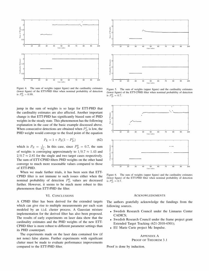
Figure 3. The sum of weights (upper figure) and the cardinality estimates(lower figure) of the ETT-CPHD filter when nominal probability of detectionis P 0

D = 0.99.

weights. The sum of the Gaussian mixture PHD weightsof ETT-CPHD and ETT-PHD algorithms along with theircorresponding cardinality estimates are shown in Figures 3and 4 respectively. Although both of the algorithms cardinalityestimates are the same, their sum of PHD weights differespecially during the occlusion of one of the targets. ETT-PHD filter has been discovered to have problems especiallywhen the target occlusion ends. When the target appearsinto the view of the sensor from behind the other target,its detection probability still remains slightly lower than thenominal probability of detection. The ETT-PHD filters sumof weights tends to grow as soon as several measurementsof the occluded target appear. This strange phenomenon canbe explained with the following basic example: Assuming nofalse alarms and a single target with existence probability PE,a single detection (without any other information than thedetection itself) should cause the expected number of targetsto be exactly unity. However, applying the standard PHDformulae, one can calculate this number to be 1+PE(1−P jD)whose bias increases as P jD decreases. We have seen that whenthe target exits the occluded region, the sudden increase inthe sum of weights appearing is a manifestation of this typeof sensitivity of the PHD filter. A similar sensitivity issue ismentioned in [12] for the case of no detection. The ETT-CPHDfilter on the other hand shows a perfect performance in thiscase.

In order to further examine the stability issues depending onlow values of the detection probability, in the second trackingexperiment, we set the nominal probability of detection toa slightly lower value P 0

D = 0.7. The results for the ETT-CPHD and ETT-PHD filters are illustrated in Figures 5 and6. respectively. We see that while the ETT-CPHD filtersperformance hardly changes, the ETT-PHD filter performanceshows remarkable differences. When the occlusion ends, the

0 10 20 30 40 50 60 70 80 90 1000

0.5

1

1.5

2

2.5

time index

Sum

ofW

eights

0 10 20 30 40 50 60 70 80 90 1000

0.5

1

1.5

2

2.5

time index

Card

inality

Est

imate

Figure 4. The sum of weights (upper figure) and the cardinality estimates(lower figure) of the ETT-PHD filter when nominal probability of detectionis P 0

D = 0.99.

jump in the sum of weights is so large for ETT-PHD thatthe cardinality estimates are also affected. Another importantchange is that ETT-PHD has significantly biased sum of PHDweights in the steady state. This phenomenon has the followingexplanation in the case of the basic example discussed above.When consecutive detections are obtained when P jD is low, thePHD weight would converge to the fixed point of the equation

PE = 1 + PE(1− P jD) (62)

which is PE = 1

P jD

. In this case, since P 0D = 0.7, the sum

of weights is converging approximately to 1/0.7 ≈ 1.43 and2/0.7 ≈ 2.85 for the single and two target cases respectively.The sum of ETT-CPHD filters PHD weights on the other handconverge to much more reasonable values compared to thoseof ETT-PHD.

When we made further trials, it has been seen that ETT-CPHD filter is not immune to such issues either when thenominal probability of detection P 0

D values are decreasedfurther. However, it seems to be much more robust to thisphenomenon than ETT-PHD the filter.

VI. CONCLUSIONS

A CPHD filter has been derived for the extended targetswhich can give rise to multiple measurements per each scanmodeled by an i.i.d. cluster process. A Gaussian mixtureimplementation for the derived filter has also been proposed.The results of early experiments on laser data show that thecardinality estimates and the PHD weights of the new ETT-CPHD filter is more robust to different parameter settings thanits PHD counterpart.

The experiments made on the laser data contained few (ifnot none) false alarms. Further experiments with significantclutter must be made to evaluate performance improvementscompared to the ETT-PHD filter.

0 10 20 30 40 50 60 70 80 90 1000

1

2

3

4

time index

Sum

ofW

eights

0 10 20 30 40 50 60 70 80 90 1000

1

2

3

4

time index

Card

inality

Est

imate

Figure 5. The sum of weights (upper figure) and the cardinality estimates(lower figure) of the ETT-CPHD filter when nominal probability of detectionis P 0

D = 0.7.

0 10 20 30 40 50 60 70 80 90 1000

1

2

3

4

time index

Sum

ofW

eights

0 10 20 30 40 50 60 70 80 90 1000

1

2

3

4

time index

Card

inality

Est

imate

Figure 6. The sum of weights (upper figure) and the cardinality estimates(lower figure) of the ETT-PHD filter when nominal probability of detectionis P 0

D = 0.7.

ACKNOWLEDGMENTS

The authors gratefully acknowledge the fundings from thefollowing sources.

• Swedish Research Council under the Linnaeus CenterCADICS;

• Swedish Research Council under the frame project grantExtended Target Tracking (621-2010-4301);

• EU Marie Curie project Mc Impulse.

APPENDIX APROOF OF THEOREM 3.1

Proof is done by induction.

• Let Z = φ, then

δ

δZGk|k−1

(pk|k−1


])= Gk|k−1

(pk|k−1


])(63)

by the definition of functional (set) derivative.• Let Z1 = {z1}, then

δ

δz1Gk|k−1

(pk|k−1


])= G

(1)k|k−1

(pk|k−1


])× pk|k−1

[pz[g])hG(1)

z PDpz(z1)]

(64)

which together with the case Z = φ proves that

δ

δZGk|k−1

(pk|k−1


])= Gk|k−1

(pk|k−1


])δZ=φ

+G(1)k|k−1

(pk|k−1


])× pk|k−1

[pz[g])hG(1)

z PDpz(z1)]

(65)

for Z = φ and Z = {z1}.Now assume that the result of Theorem 3.1 holds for

Zn−1 = {z1, . . . , zn−1}, n ≥ 2. Then we are going to seewhether the result holds of Zn = Zn−1 ∪ zn.

δ

δZn−1 ∪ znGk|k−1

(pk|k−1


])=

δ

δzn

δ

δZn−1Gk|k−1

(pk|k−1


])(66)

=δ

δzn

(Gk|k−1

(pk|k−1


])δZn−1=φ

+∑

P∠Zn−1

G(|P|)k|k−1

(pk|k−1


])×∏W∈P

pk|k−1

[hPDG

|W |z (pz[g])

∏z′∈W

pz(z′)

])(67)

=δ

δzn

∑P∠Zn−1

G(|P|)k|k−1

(pk|k−1


])×∏W∈P

pk|k−1

[hPDG

|W |z (pz[g])

∏z′∈W

pz(z′)

](68)

=∑

P∠Zn−1

(G

(|P|+1)k|k−1

(pk|k−1


])× pk|k−1

[hPDG

(1)z (pz[g]))pz(zn)

]×∏W∈P

pk|k−1

[hPDG

|W |z (pz[g])

∏z′∈W

pz(z′)

]+G

(|P|)k|k−1

(pk|k−1


])×∑W∈P

pk|k−1

[hPDG

|W |+1z (pz[g])

∏z′∈W∪zn

pz(z′)

]

×∏

W ′∈P−Wpk|k−1

[hPDG

|W ′|z (pz[g])

∏z′∈W ′

pz(z′)

])(69)

=∑

P∠Zn−1

(G

(|P|+1)k|k−1

(pk|k−1


])×

∏W∈P∪{zn}

pk|k−1

[hPDG

|W |z (pz[g])

∏z′∈W

pz(z′)

]+G

(|P|)k|k−1

(pk|k−1


])×∑W∈P

∏W ′∈P−W∪(W∪zn)

× pk|k−1

[hPDG

|W ′|z (pz[g])

∏z′∈W ′

pz(z′)

])(70)

=∑

P∠Zn−1∪zn

G(|P|)k|k−1

(pk|k−1


])×∏W∈P

pk|k−1

[hPDG

|W |z (pz[g])

∏z′∈W

pz(z′)

](71)

which is equal to

δ

δZnGk|k−1

(pk|k−1


])(72)

by the result of Theorem 3.1. The proof is complete. �

APPENDIX BPROOF OF THEOREM 3.2

Substituting the result of Theorem 3.1 into (22), we obtain

δ

δZF [g, h] =

∑S⊆Z

δ


×

(Gk|k−1

(pk|k−1


])δS=φ

+∑P∠S

G(|P|)k|k−1

(pk|k−1


])×∏W∈P

pk|k−1

[hPDG

|W |z (pz[g])

∏z′∈W

pz(z′)

])(73)

=δ

δZGFA(pFA[g])

×Gk|k−1

(pk|k−1


])+∑S⊆Z

δ


×∑P∠S

G(|P|)k|k−1

(pk|k−1


])×∏W∈P

pk|k−1

[hPDG

|W |z (pz[g])

∏z′∈W

pz(z′)

](74)

=

(∏z′∈Z

pFA(z′)

)(G

(|Z|)FA (pFA[g])

×Gk|k−1

(pk|k−1


])

+∑S⊆Z

G(|Z−S|)FA (pFA[g])

×∑P∠S

G(|P|)k|k−1

(pk|k−1


])×∏W∈P

pk|k−1

[hPDG

|W |z (pz[g])

∏z′∈W

pz(z′)

pFA(z′)

])(75)

=

(∏z′∈Z

pFA(z′)

)(G

(|Z|)FA (pFA[g]) (76)

×Gk|k−1

(pk|k−1


])+GFA(pFA[g])

×∑P∠Z

G(|P|)k|k−1

(pk|k−1


])×∏W∈P

pk|k−1

[hPDG

|W |z (pz[g])

∏z′∈W

pz(z′)

pFA(z′)

]+∑S⊂ZS 6=Z

G(|Z−S|)FA (pFA[g])

×∑P∠S

G(|P|)k|k−1

(pk|k−1


])×∏W∈P

pk|k−1

[hPDG

|W |z (pz[g])

∏z′∈W

pz(z′)

pFA(z′)

])(77)

=

(∏z′∈Z

pFA(z′)

)(G

(|Z|)FA (pFA[g])

×Gk|k−1

(pk|k−1


])+GFA(pFA[g])

×∑P∠Z

G(|P|)k|k−1

(pk|k−1


])×∏W∈P

pk|k−1

[hPDG

|W |z (pz[g])

∏z′∈W

pz(z′)

pFA(z′)

]+∑P∠Z|P|>1

∑W∈P

G(|W |)FA (pFA[g])

×G(|P|−1)k|k−1

(pk|k−1


])×

∏W ′∈P−W

pk|k−1

[hPDG

|W ′|z (pz[g])

∏z′∈W ′

pz(z′)

pFA(z′)

])(78)

where we used the equality

∑S⊂ZS 6=Z

f(Z − S)∑P∠S

g(P) =∑P∠Z|P|>1

∑W∈P

f(W )g(P −W )

(79)

while going from (77) to (78). Now, including the multiplica-tion

G(|Z|)FA (pFA[g])Gk|k−1

(pk|k−1


])(80)

into the summation∑P∠Z|P|>1

as the case of |P| = 1, i.e., P =

{Z} with the convention that∏W∈φ = 1, we get

δ

δZF [g, h] =

(∏z′∈Z

pFA(z′)

)(GFA(pFA[g])

×∑P∠Z

G(|P|)k|k−1

(pk|k−1


])×∏W∈P

pk|k−1

[hPDG

|W |z (pz[g])

∏z′∈W

pz(z′)

pFA(z′)

]+∑P∠Z

∑W∈P

G(|W |)FA (pFA[g])

×G(|P|−1)k|k−1

(pk|k−1


])×

∏W ′∈P−W

pk|k−1

[hPDG

|W ′|z (pz[g])

∏z′∈W ′

pz(z′)

pFA(z′)

])(81)

=

(∏z′∈Z

pFA(z′)

)( ∑P∠Z

GFA(pFA[g])

×G(|P|)k|k−1

(pk|k−1


])×∏W∈P

pk|k−1

[hPDG

|W |z (pz[g])

∏z′∈W

pz(z′)

pFA(z′)

]+∑P∠Z

∑W∈P

G(|W |)FA (pFA[g])

×G(|P|−1)k|k−1

(pk|k−1


])×

∏W ′∈P−W

pk|k−1

[hPDG

|W ′|z (pz[g])

∏z′∈W ′

pz(z′)

pFA(z′)

])(82)

=

(∏z′∈Z

pFA(z′)

) ∑P∠Z

(GFA(pFA[g])

×G(|P|)k|k−1

(pk|k−1


])× 1

|P|∑W∈P

pk|k−1

[hPDG

|W |z (pz[g])

∏z′∈W

pz(z′)

pFA(z′)

]×

∏W ′∈P−W

pk|k−1

[hPDG

|W ′|z (pz[g])

∏z′∈W ′

pz(z′)

pFA(z′)

]+∑W∈P

G(|W |)FA (pFA[g])

×G(|P|−1)k|k−1

(pk|k−1


])×

∏W ′∈P−W

pk|k−1

[hPDG

|W ′|z (pz[g])

∏z′∈W ′

pz(z′)

pFA(z′)

])(83)

=

(∏z′∈Z

pFA(z′)

) ∑P∠Z

∑W∈P

(GFA(pFA[g])

×G(|P|)k|k−1

(pk|k−1


])× 1

|P|pk|k−1

[hPDG

|W |z (pz[g])

∏z′∈W

pz(z′)

pFA(z′)

]+G

(|W |)FA (pFA[g])

×G(|P|−1)k|k−1

(pk|k−1


]))

×∏

W ′∈P−Wpk|k−1

[hPDG

|W ′|z (pz[g])

∏z′∈W ′

pz(z′)

pFA(z′)

](84)

which is the result of Theorem 3.2 when we substitute theterms ηW [g, h] defined in (24). Proof is complete. �

APPENDIX CPROOF OF THEOREM 3.3

Taking the derivative of both sides of (27), we get

δ

δx

δ

δZF [0, h] =

(∏z′∈Z

pFA(z′)

)pk|k−1(x)

×∑P∠Z

∑W∈P

( ∏W ′∈P−W

ηW ′ [0, h]

)

×

(GFA(0)G

(|P|+1)k|k−1 (ρ[h])(1− PD(x) + PD(x)Gz(0))

× ηW [0, h]

|P|+GFA(0)G

(|P|)k|k−1(ρ[h])

h(x)PD(x)G|W |z (0)

|P|

×∏z′∈W

pz(z′|x)

pFA(z′)+G

(|W |)FA (0)G

(|P|)k|k−1(ρ[h])

× (1− PD(x) + PD(x)Gz(0))

+

(GFA(0)G

(|P|)k|k−1(ρ[h])

ηW [0, h]

|P|

+G(|W |)FA (0)G

(|P|−1)k|k−1 (ρ[h])

)×

∑W ′∈P−W


ηW ′ [0, h]

∏z′∈W ′

pz(z′|x)

pFA(z′)

)(85)

=

(∏z′∈Z

pFA(z′)

)pk|k−1(x)

×∑P∠Z

∑W∈P

( ∏W ′∈P−W

ηW ′ [0, h]

)

×

((GFA(0)G

(|P|+1)k|k−1 (ρ[h])

ηW [0, h]

|P|

+G(|W |)FA (0)G

(|P|)k|k−1(ρ[h])

)(1− PD(x) + PD(x)Gz(0))

+GFA(0)G(|P|)k|k−1(ρ[h])

h(x)PD(x)G|W |z (0)

|P|∏z′∈W

pz(z′|x)

pFA(z′)

+

(GFA(0)G

(|P|)k|k−1(ρ[h])

ηW [0, h]

|P|

+G(|W |)FA (0)G

(|P|−1)k|k−1 (ρ)

)×

∑W ′∈P−W


ηW ′ [0, h]

∏z′∈W ′

pz(z′|x)

pFA(z′)

)(86)

which is the result of Theorem 3.3. The proof is complete.�

APPENDIX DREDUCING ETT-CPHD TO ETT-PHD

When one constrains all the processes to Poisson, we get thefollowing identities.

G(n)FA(x) =λnG

(n)FA(x) (87)

G(n)z (x) =τnG(n)

z (x) (88)

G(n)k|k−1(x) =Nn

k|k−1G(n)k|k−1(x) (89)

where λ and τ are the expected number of false alarms andmeasurements from a single target. Nk|k−1 is the predictedexpected number of targets i.e., Nk|k− 1 =

∫Dk|k−1(x) dx.

We are first going to examine the constant κ defined in (37).For this purpose, we first write

βP,W ,GFA(0)Gk|k−1(ρ[1])

(N|P|k|k−1

ηW [0, 1]

|P|

+ λ|W |N|P|−1k|k−1

); (90)

γP,W ,GFA(0)Gk|k−1(ρ[1])

(N|P|+1)k|k−1

ηW [0, 1]

|P|

+ λ|W |N|P|k|k−1

). (91)

Now, substituting these into (37), we get

κ =

∑P∠Z

∑W∈P αP,W

×(N|P|+1k|k−1

ηW [0,1]|P| + λ|W |N

|P|k|k−1

)∑P∠Z

∑W∈P αP,W

×(N|P|k|k−1

ηW [0,1]|P| + λ|W |N

|P|−1k|k−1

) = Nk|k−1. (92)

We here define the modified versions of ηW [0, 1], and αP,Was

ηW [0, 1] ,Nk|k−1ηW [0, 1]

λ|W |(93)

=Dk|k−1

[PDG

(|W |)z (0)

∏z′∈W

pz(z′)

λpFA(z′)

](94)

αP,W ,N|P |−1k|k−1λ

|W |αP,W [0, 1] (95)

=λ|Z|∏

W ′∈P−WηW ′ [0, 1]. (96)

With these definitions βP,W and the multiplicationαP,WβP,W become

βP,W ,GFA(0)Gk|k−1(ρ[1])N|P|−1k|k−1λ

|W |

×(ηW [0, 1]

|P|+ 1

)(97)

αP,WβP,W =GFA(0)Gk|k−1(ρ[1])αP,W

×(ηW [0, 1]

|P|+ 1

). (98)

Using these, we can write σP,W as

σP,W ,G|W |z (0)GFA(0)Gk|k−1(ρ[1])Nk|k−1λ

−|W |(αP,W|P|

+

∑W ′∈P−W αP,W ′

( ηW ′ [0,1]|P| + 1

)ηW [0, 1]

). (99)

After defining the quantity ζP as

ζP ,∏W∈P

ηW [0, 1] = αP,W ηW [0, 1], (100)

we can turn (99) into

σP,W ,G|W |z (0)GFA(0)Gk|k−1(ρ[1])Nk|k−1λ

−|W |

×ζP + |P|

∑W ′∈P−W αP,W ′

( ηW ′ [0,1]|P| + 1

)|P|ηW [0, 1]

(101)

=G|W |z (0)GFA(0)Gk|k−1(ρ[1])Nk|k−1λ−|W |

×|P|ζP + |P|

∑W ′∈P−W ζP−W ′

|P|ηW [0, 1](102)


×ζP +

∑W ′∈P−W ζP−W ′

ηW [0, 1](103)


×(ζP−W +

∑W ′∈P−W

ζP−W−W ′

)(104)

=e−ττ |W |GFA(0)Gk|k−1(ρ[1])Nk|k−1λ−|W |

×(ζP−W +

∑W ′∈P−W

ζP−W−W ′

). (105)

We can write by using (105) and (98)σP,W∑


=

(Nk|k−1e

−ττ |W |λ−|W |

×(ζP−W +

∑W ′∈P−W ζP−W−W ′

) )∑P∠Z

∑W∈P αP,W

(ηW [0,1]|P| + 1

) (106)

= Nk|k−1

(e−ττ |W |λ−|W |

×(ζP−W +

∑W ′∈P−W ζP−W−W ′

) )∑P∠Z

(ζP +

∑W∈P ζP−W

) .

(107)

Substituting (107) into the update equation (39) forDk|k−1( · ), we get

Dk|k(x) =(1− PD(x) + PD(x)Gz(0))Dk|k−1(x)

+ e−τ

∑P∠Z

∑W∈P

(ζP−W

+∑W ′∈P−W ζP−W−W ′

)×τ |W |

∏z′∈W

pz(z′|x)λpFA(z′)PD(x)

∑P∠Z

(ζP +

∑W∈P ζP−W

) Dk|k−1(x).

(108)

• First, we examine the term∑P∠Z

(ζP +

∑W∈P ζP−W

)in the denominator of (108) as follows.∑P∠Z

(ζP +

∑W∈P

ζP−W

)=∑P∠Z

ζP +∑P∠Z

∑W∈P

ζP−W

(109)

=∑P∠Z

ζP +∑P∠Z|P|>1

∑W∈P

ζP−W + 1.

(110)

If we use the identity (79) on the second term in thesummation on the right hand side of (110), we obtain∑P∠Z

(ζP +

∑W∈P

ζP−W

)=∑P∠Z

ζP +∑S⊂ZS 6=Z

∑P∠S

ζP + 1

(111)

=∑S⊂Z

∑P∠S

ζP + 1 (112)

=∑P∠Z

∏W∈P

dW (113)

where

dW =δ|W |=1 + ηW [0, 1]. (114)

• We examine the numerator term in (108) below.∑P∠Z

∑W∈P

gnum(P −W )fnum(W ) (115)

where we defined

fnum(W ) ,τ |W |∏z′∈W

pz(z′|x)

λpFA(z′)PD(x) (116)

gnum(P) ,(ζP +

∑W ′∈P

ζP−W ′). (117)

Separating the case P = {Z} from the summation in(115), we get∑P∠Z

∑W∈P

gnum(P −W )fnum(W ) =fnum(Z)

+∑P∠Z|P|>1

∑W∈P

gnum(P −W )fnum(W ) (118)

= fnum(Z) +∑S⊂ZS 6=Z

fnum(S −W )∑P∠S

gnum(P).

(119)

where we used the identity (79). Now realizing that wecalculated the term

∑P∠Z gnum(P) as in (113), we can

substitute this into (119) as follows.∑P∠Z

∑W∈P


+∑S⊂ZS 6=Z

fnum(S −W )∑P∠S

∏W∈P

dW

(120)

Resorting to the identity (79) once again, we get∑P∠Z

∑W∈P


+∑P∠Z|P|>1

∑W∈P

fnum(W )∏

W ′∈P−WdW ′ (121)

=∑P∠Z

∑W∈P

fnum(W )∏

W ′∈P−WdW ′ . (122)

When we substitute the results (113) and (122) back into (108),we obtain

Dk|k(x) =

((1− PD(x) + PD(x)Gz(0))

+ e−τ∑P∠Z

ωP∑W∈P

τ |W |

dW

∏z′∈W

pz(z′|x)

λpFA(z′)PD(x)

)×Dk|k−1(x) (123)

where

ωP ,

∏W∈P dW∑

P∠Z∏W∈P dW

(124)

which is the same PHD update equation as in [6, equation(5)]. Moreover, the terms dW and ωP are the same as thosedefined in [6, equations (7) and (6) respectively].

REFERENCES

[1] K. Gilholm and D. Salmond, “Spatial distribution model for trackingextended objects,” IEE Proceedings Radar, Sonar and Navigation, vol.152, no. 5, pp. 364–371, Oct. 2005.

[2] K. Gilholm, S. Godsill, S. Maskell, and D. Salmond, “Poisson modelsfor extended target and group tracking,” in Proceedings of Signal andData Processing of Small Targets, vol. 5913. San Diego, CA, USA:SPIE, Aug. 2005, pp. 230–241.

[3] Y. Boers, H. Driessen, J. Torstensson, M. Trieb, R. Karlsson, andF. Gustafsson, “A track before detect algorithm for tracking extendedtargets,” IEE Proceedings Radar, Sonar and Navigation, vol. 153, no. 4,pp. 345–351, Aug. 2006.

[4] R. Mahler, “Multitarget Bayes filtering via first-order multi targetmoments,” vol. 39, no. 4, pp. 1152–1178, Oct. 2003.

[5] B.-N. Vo and W.-K. Ma, “The Gaussian mixture probability hypothesisdensity filter,” IEEE Trans. Signal Process., vol. 54, no. 11, pp. 4091–4104, Nov. 2006.

[6] R. Mahler, “PHD filters for nonstandard targets, I: Extended targets,”in Proceedings of the International Conference on Information Fusion,Seattle, WA, USA, Jul. 2009, pp. 915–921.

[7] K. Granstrom, C. Lundquist, and U. Orguner, “A Gaussian mixturePHD filter for extended target tracking,” in Proceedings of InternationalConference on Information Fusion, Edinburgh, Scotland, May 2010.

[8] R. Mahler, “PHD filters of higher order in target number,” IEEE Trans.Aerosp. Electron. Syst., vol. 43, no. 4, pp. 1523–1543, Oct. 2007.

[9] ——, personal correspondence, Oct. 2010.

[10] U. Orguner. (2010, Nov.) CPHD filter derivation for extendedtargets. ArXiv:1011.1512v2. [Online]. Available: http://arxiv.org/abs/1011.1512v2

[11] R. Mahler, Statistical Multisource-Multitarget Information Fusion, Nor-wood, MA, USA, 2007.

[12] O. Erdinc, P. Willett, and Y. Bar-Shalom, “The bin-occupancy filter andits connection to the PHD filters,” vol. 57, no. 11, pp. 4232 –4246, Nov.2009.

Avdelning, Institution

Division, Department

Division of Automatic ControlDepartment of Electrical Engineering

Datum

Date

2011-03-14

Språk

Language

� Svenska/Swedish

� Engelska/English

�

�

Rapporttyp

Report category

� Licentiatavhandling

� Examensarbete

� C-uppsats

� D-uppsats

� Övrig rapport

�

�

URL för elektronisk version


ISBN

�

ISRN

�

Serietitel och serienummer

Title of series, numberingISSN

1400-3902

LiTH-ISY-R-2999

Titel

TitleExtended Target Tracking with a Cardinalized Probability Hypothesis Density Filter

Författare

AuthorUmut Orguner, Christian Lundquist, Karl Granström

Sammanfattning

Abstract

This technical report presents a cardinalized probability hypothesis density (CPHD) �lterfor extended targets that can result in multiple measurements at each scan. The probabilityhypothesis density (PHD) �lter for such targets has already been derived by Mahler and aGaussian mixture implementation has been proposed recently. This work relaxes the Poissonassumptions of the extended target PHD �lter in target and measurement numbers to achievebetter estimation performance. A Gaussian mixture implementation is described. The earlyresults using real data from a laser sensor con�rm that the sensitivity of the number of targetsin the extended target PHD �lter can be avoided with the added �exibility of the extendedtarget CPHD �lter.

Nyckelord

Keywords Multiple target tracking, extended targets, random sets, probability hypothesis density, car-dinalized, PHD, CPHD, Gaussian mixture, laser.


Extended Target Tracking with a Cardinalized...

Documents

Transcript of Extended Target Tracking with a Cardinalized...