Extended Job Shop Scheduling by Object-Oriented

Optimization Technology∗

Minoru Kobayashi, Kenji Muramatsu

Tokai University

Address: 1117 Kitakaname, Hiratsuka, Kanagawa, 259-1292, Japan

Telephone: +81-463-58-1211 ext. 4486, Facsimile: +81-463-50-2055

E-mail: {kobayam, kenji}@keyaki.cc.u-tokai.ac.jp

Abstract

Almost all conventional benchmarking problems of Job Shop Scheduling Problem

(JSSP) are not realistic in the sense that interruptions of operations, uses of alternative

machines and so on are not allowed. Its theory is also mainly confined to treat just

only the decision feature of sequencing. Then, we advocate an extended model of JSSP

involving various heterogeneous decision features such as lot splitting (interruption of

operation), dispatching as well as sequencing. Consequently, the problem has a feature

∗Abstract number: 002-0516, Name of the Conference: Second World Conference on POM and 15th

Annual POM Conference, Cancun, Mexico, April 30 - May 3, 2004.

1

of combinatorial and continuous dynamic optimization and hence the extension of

solution concept and a new solution principle is obligatory. One of the key ideas

approaching to this new type of problem is to introduce the concept of progress of

operations into the model and to formulate it into a transient state in a dynamic

optimization problem. Then, we present the methodology denominated the object

oriented optimization technology that enables to optimize (near optimize precisely)

all of those decision features.

1 Introduction

1.1 The objective

This paper presents the concept of extended job shop scheduling problem. The aim is

to reflect real job shop scheduling situation on the field of our study and to present a

direction for bridging the gap between theory of scheduling and practice.

In fact, in this type of real problem, there exist various heterogeneous decision features,

and, as shown later, there exists a big room for developing a reasonable methodology so

as to be able to deal with those decision features.

Then, it presents a methodology that deals with all of them simultaneously from the

viewpoint of global optimization.

It consists of a fine mathematical model that enables us to formulate all of the decision

features, a new principle of global optimization, and an algorithm to reduce cpu time,

which we call the Object-Oriented Optimization Technology (O2O-Technology).

2

1.2 Review

So far, there has not been seen the paper that solves all of the heterogeneous decision fea-

tures involved in an extended job shop scheduling problem (EJSSP) simultaneously. Some

of the decision features belong to the category of combinatorial or discrete optimization

and the other to the continuous optimization.

So, as known also from that the conventional mathematics is split into two categories

of discrete mathematics and continuous one, it is difficult to solve this type of optimization

problem that has both features in a mathematical sense too.

As to multi-item multi-process dynamic lot size scheduling problem (MIMPDLSP),

already the approach similar to the one that we will present to EJSSP in this paper has

been presented in [1] [2].

Therefore, if the trial that we present in this paper succeeds, it will leads to verify the

potential of the methodology that we call O2O-Technology to a wide variety of scheduling

problems[3].

1.3 Contents

In section 2, we mention the characteristics and the difference between classical job shop

scheduling problem and extended job shop scheduling problem. In section 3, we present

the core concept of O2O-Technology and the relation between extended job shop shcedul-

ing problem and multi-item multi-process dynamic lot size shceduling problem. Section

4 and 5 presents the mathematical model of extended job shop scheduling problem and its

solution algorithm by Lagrangian decomposition coordination method. Section 6 shows

3

an illustration of numerical experimentation. In section 7, we point out a few drawbacks

as well as some advantages of this solution method. Lastly, we conclude this paper.

2 Job shop scheduling problem and its extention

2.1 Classical JSSP

We will begin with clarifying the difference between the existent (classical) job shop

scheduling problem (JSSP) and the extended one (EJSSP.) As well known, fundamentally,

existent JSSP is to determine the sequence of the tasks on each machine. The definition of

JSSP at page 273 in [4] is the following: A job shop consists of a set of different machines

that perform tasks of jobs. Each job has a specified processing order through the machines,

i.e. a job is composed of an ordered list of tasks each of which is determined by the machine

required and the processing time on it. There are several constraints on jobs and machines;

(1) There are no precedence constraints among tasks of different jobs; (2) tasks cannot be

interrupted (non-preemption) and each machine can handle only one job at a time; (3)

each job can be performed only one machine at a time. While the machine sequence of the

jobs is fixed, the problem is to find the jobs sequence on the machines which minimize the

makespan., i.e. the maximum of the completion times of all tasks. However, in a real job

shop scheduling environment, sequencing is just only one of various decision features.

Especially, the environment of the present is not so simple because real time nature, high

resolution, and global optimization are required in management field also.

4

2.2 Extended job shop scheduling problem

Here, we define the extended job shop scheduling problem (EJSSP.) For this aim, we

consider the features to be treated newly and the way of treatment in the EJSSP.

Alternative machine

Usually, there exist alternative machine or machines. Therefore, the feature of assign-

ment, dispatching, or loading is added to the decision features other than the one of JSSP.

In addition, usually, processing time depends on the machine for use.

Repetitive order or shipment requirements

Even if it is job shop scheduling environment, it is not unusual that the same item or

job is ordered repeatedly and yet its quantity also differs. It implies that the concept of

stock is related to the problem.

In other wards, it would mean that we could not solve the problem unless we treat

transition of stock in explicit in the model. Such treatment would be rather natural because

processing and stock as its result are closely related and in a real situation almost always

they are concerned with these features.

Preemption or lot splitting

If an urgent order is placed, it is also quite natural to interrupt the processing of the task

on a machine and start the processing of the task of the order. The concept of preemption is

equivalent to the one of lot splitting in flow shop scheduling in mathematical formulation

as shown later.

Set up cost and time

Whether preemption is allowed or not is closely related to set up time and cost. In

5

a case when physically interruption of a processing is not allowed, it is able to avoid it

by setting the set up cost at a constant of a very large value in the model. Like this, in

formulating the situation, the objective function or the criteria of the problem also play a

role together with constants.

Jumping the gun is allowed, i.e. the processing of the next task is started before a task

is completed

Clearly, there exists a case when jumping is allowed and the one not so. If it is allowed,

the decision feature of at what time it is started should be added newly. This decision

affects its stock transition.

Therefore, we define EJSSP as the problem that has the features mentioned here as

well as the one of JSSP. However, as to the criteria of the problem, we will confine it to the

one that has additively separable property with respect to item or task. Concretely, for

example, the problem to minimize the maximum makespan is not additively separable. In

the approach that we present, we take advantage of additively separable property common

to almost all scheduling problems to decompose the whole optimization problem of large

scale into item or task base sub-optimization problems.

6

3 Analysis of EJSSP and prerequisites for new methodol-

ogy

3.1 Characteristics of actual requests in EJSSP

As mentioned above, in a real EJSSP the various heterogeneous decision features such

as dispatching, loading, lot sizing, as well as sequencing are mingled with each other.

And yet it is hard to separate them into individual features. Moreover, the problems are

extended over a wide variety of cases by combinations of system elements or features.

Furthermore, the requests of today for real time nature, high resolution, and global

optimization in management technology have become much higher because of advance

of information and communication technology and high technology and so on.

However, as the conventional approach is mainly focused on the optimization of a

certain decision feature, its application to a problem with an extended feature or features

is extremely difficult.

The way of solving each of the decision features by its corresponding method one by

one in turn and integrating them later also would not suit the requirements of the present.

3.2 Core concept of the new methodology

Then, in this paper, we will innovate the concept of solution methodology. Namely, we

will deal with all of the decision features simultaneously and yet unconsciously from the

viewpoint of global optimization. We begin with the explanation of the core concept.

As well known, it has been seen the tendency that if we adhere to any one of the

7

decision features and want to solve it, it becomes more difficult to solve the other together

with it. So, we will avoid this sort of drawback of the existent methodology at the first

stage of problem solution. That is, at the stage of formulation, we adopt a means to

formulate the problem as finely as possible without adhering to any decision feature. This

is the core concept.

For this aim, as decision variables, we use only 0-1 variables that we call primitive

objects. Each primitive object has many suffices, each of which corresponds to an object

such as an item (or task), machine, or time slot. Therefore, the decision variable itself

denotes only the state of the processing that is specified by suffices, and alone it does

not denote any of the decision features such as sequencing, task splitting (lot sizing),

dispatching, or jumping.

As for problem formulation by using 0-1 decision variables, many papers have been

presented already. However, a big difference is that in the approach presented in this

paper, any 0-1 decision variable alone does not correspond to any of the decision features.

As shown later, the formulation by use of various primitive objects enables to solve all

of the decision features simultaneously and yet without paying attention to any of them

from the viewpoint of global optimization mentioned above.

3.3 Prerequisites

Below, we put on the three prerequisites for satisfying all requirements.

• fine mathematical model to formulate the details

• new principle enables to optimize heterogeneous decision features simultaneously

8

• reduction of computational time

The object oriented optimization technology (O2O-Technology) that we advocate has

all of those prerequisites.

Therefore, it would have the high potential of application to a wide variety of schedul-

ing problems involving EJSSP.

Then, we will present the method of solving EJSSP assuming the O2O-Technology.

3.4 Classification of EJSSP and its relation to MIMPDLSP

Before formulation, we need to analyze EJSSP from the viewpoint of applying the O2O-

Technology to it. The aim is to clarify the characteristics inherent to the EJSSP and its

difference from MIMPDLSP. The end is to specify the module to be built into the model

of EJSSP newly and the ones common to MIMPDLSP.

We take the new features to be treated and the relations with the treatment in MIMPDLSP.

Alternative machine: Its treatment is the same as in the case of MIMPDLSP.

Repetitive order or shipment requirements: It is also the same as in case of MIMPDLSP.

Set up cost and time: As to these, we are able to build it into the objective function in the

same as in case of MIMPDLSP.

As to preemption and jumping, the treatments differ from the one of above features

and depend on the combination of them (shown in Figure 1).

(1) Non-preemption and non-jumping: In case of no alternative machines and no repet-

itive shipment requirements, it corresponds to the classical JSSP.

(2) Non preemption and jumping: This feature is new.

9

MachinebT

Machineb3

Machineb4

Machinebk

MachinebT

Machineb3

Machineb4

Machinebk

MachinebT

Machineb3

Machineb4

Machinebk

MachinebT

Machineb3

Machineb4

Machinebk

Caseb(k):bNon-preemptionbandbnon-jumping Caseb(T):bNon-preemptionbandbjumping

Caseb(3):bPreemptionbandbnon-jumping Caseb(4):bPreemptionbandbjumping

Jumpingbthebgunboccured

Preemptionboccured Preemptionbandbjumpingbthebgunboccured

Figure 1: An instance of preemption and jumping in EJSSP

(3) Preemption and non-jumping: This feature is also new.

(4) Preemption and jumping: Regardless of alternative machine and/or repetitive ship-

ment requirements, the problem itself is equivalent to the MIMPDLSP, and hence

the existent model for MIMPDLSP is applied to this problem without any additional

treatment.

However, as to the criteria, it is confined to the one that has additively separable

property for the reason mentioned in section 2.2. As to details, we will treat in section 5.

4 Mathematical model of EJSSP

The Lagrangian of this problem is given as follows.

L(δ, x, s;λ, µ, κ) =∑

i∈I

∑

t∈T

(∑

k∈K(i)

cki (1 − δk

i,t−1)δkit + hixit

)+

∑

k∈K

∑

t∈Tλkt

( ∑

i∈M(k)

δkit − 1

)

+∑

i∈I

∑

t∈Tµit

((xi+1,t − xi+1,0) − xit

)+

∑

j∈J

∑

t∈Tκ jt

(∑

i∈I( j)

δkit − 1

)(1)

10

The first term is the total cost of set up cost and inventory holding cost over the planning

horizon. The second, the third and the forth term corresponds to the constraints of the

machine interference, work-in-process inventory shortage and of simultaneous operation

weighted with penalty cost respectively.

The notations used in (1) are following:

Notations

J = {1, 2, . . . , l − 1, l} : set of jobs.

I = {1, 2, . . . ,m − 1,m} : set of tasks.

T = {1, 2, . . . , n − 1,n} : set of time slots.

K = {1, 2, . . . , q − 1, q} : set of machines.

M(k) : set of task i ∈ I using machine k ∈ K.

K(i) : set of machine k ∈ K operates task i ∈ I.

I( j) : set of task i ∈ I involved job j ∈ J.

J(i) : set of jobs j ∈ J have task i ∈ I.

cki : set up cost to task i ∈ I using machine k ∈ K.

ski : set up time to task i ∈ I using machine k ∈ K.

sit : remaining time of set up of task i ∈ I using machine k ∈ K. si is a vector whose elements

are sit,∀t ∈ T, and s is a vector whose elements are si,∀i ∈ I

pki : production ability of task i ∈ I using machine k ∈ K per unit time slot.

xit : inventory of task i ∈ I at the end of t ∈ T. xi is a vector whose elements are xit,∀t ∈ T,

and x is a vector whose elements are xi,∀i ∈ I.

xi min, xi max : lower and upper limit of inventory level for each i ∈ I.

hi : rate of inventory holding cost of task i ∈ I per unit time slot.

11

r jt : shipment requirement of job j ∈ J at due time t ∈ T, this is given for the last task in

each job.

δkit : binary decision variable that takes value 1 if a machine k processes task i at time slot t,

else takes 0. δi is a vector whose elements are δkit,∀t ∈ T,∀k ∈ K(i), and δ is a vector whose

elements are δi,∀i ∈ I.

I(sit) : index function that takes value 1 if sit = 0, else 0.

λkt : Lagrange multiplier (for machine interference constraint). λ is a vector whose elements

are λkt,∀k ∈ K,∀t ∈ T.

µit : Lagrange multiplier (for work-in-process inventory shortage constraint). µ is a vector

whose elements are µit,∀i ∈ I,∀t ∈ T.

κ jt : Lagrange multiplier (for simultaneous task operation constraint). κ is a vector whose

elements are κ jt,∀ j ∈ J,∀t ∈ T.

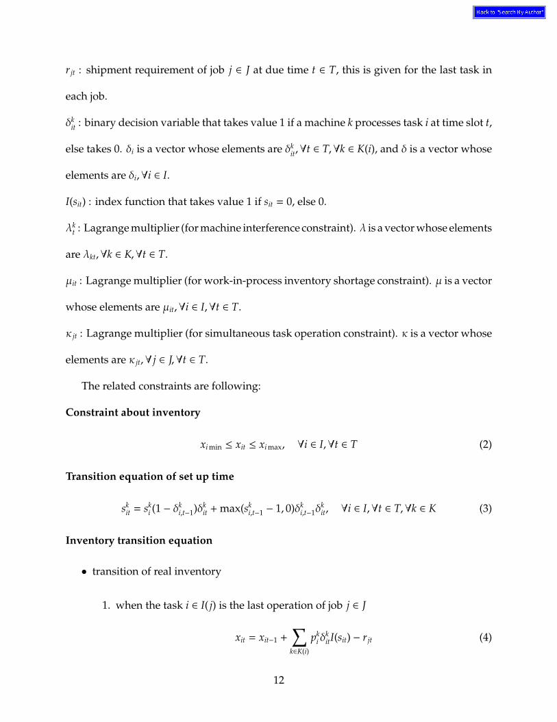
The related constraints are following:

Constraint about inventory

xi min ≤ xit ≤ xi max, ∀i ∈ I,∀t ∈ T (2)

Transition equation of set up time

skit = sk

i (1 − δki,t−1)δk

it + max(ski,t−1 − 1, 0)δk

i,t−1δkit, ∀i ∈ I,∀t ∈ T,∀k ∈ K (3)

Inventory transition equation

• transition of real inventory

1. when the task i ∈ I( j) is the last operation of job j ∈ J

xit = xit−1 +∑

k∈K(i)

pki δ

kitI(sit) − r jt (4)

12

2. when the task i ∈ I( j) is not the last operation of job j ∈ J

xit = xit−1 +∑

k∈K(i)

pki δ

kitI(sit) −

∑

k′∈K(i+1)

pk′i+1δ

k′i+1,tI(si+1,t) (5)

• transition of echelon inventory is same as equation (4) of transition of real inventory.

Constraint of prohibition of machine interference

∑

i∈M(k)

δkit ≤ 1, ∀t ∈ T,∀k ∈ K (6)

Constraint of prohibition of shortage of work-in-process inventory

xi+1,t − xi+1,0 ≤ xit, ∀i ∈ I( j),∀t ∈ T,∀ j ∈ J (7)

Constraint of prohibition of simultaneous task opration for each job

∑

i∈I( j)

δkit ≤ 1, ∀k ∈ K(i),∀t ∈ T,∀ j ∈ J (8)

Objective function

f (δ, x) =∑

i∈I

∑

t∈T

(∑

k∈K(i)

cki (1 − δit−1)δit + hixit

)(9)

5 Algorithm

The Lagrangian (1) is separable. Consequently putting Li(δi, xi, si;λ, µ, κ) as

Li(δi, xi, si;λ, µ, κ) =∑

t∈T

(∑

k∈K(i)

cki (1 − δk

i,t−1)δkit + hixit

)+

∑

k∈K(i)

∑

t∈Tλktδ

kit

−∑

t∈T

(µit − µi−1,t

)xit +

∑

j∈J(i)

∑

t∈Tκ jtδ

kit (10)

So, we can decompose the Lagrangian into task-based sub-optimization problems as

follows.

13

Sub-optimization problem

minδi

Li(δi, xi, si;λ, µ, κ)

subject to (2) − (5)(11)

The algorithm is as follows:

Step 1 Initialize the Lagrange multipliers.

Step 2 Solve sub-optimization problems for all tasks i ∈ I by dynamic programming.

Step 3 Calculate the perturbation of interaction constraint.

Step 4 If all constraint is satisfied, then stop, else go to Step 5.

Step 5 Update the Lagrange multipliers based on the quantity of perturbation, and go

back to Step 2.

In this paper, we update the Lagrange multipliers by monotonely non-decreasing rule

based on subgradient method below.

λν+1kt := λνkt + αkk1 max

( ∑

i∈M(k)

δkit − 1, 0

)(12)

µν+1it := µνit + βik1k2 max

((xi+1,t − xi+1,0

) − xit, 0)

(13)

κν+1jt := κνjt + γ jk1 max

( ∑

i∈I( j)

δkit − 1, 0

)(14)

where ν denotes the number of iteration in computation and αk, βi, γ j, k1 and k2 are step

length and coordinating parameter respectively. For the detail of configuring them, cf.

[5].

14

������� ������� ������� �������

MaMMac Mah

Mai caMcac

cahcai hah

hac

haMhai

iac

iah

iaM

iai

Mac

nebaT34k

Figure 2: System diagram

6 Numerical illustration

We illustrate the extended job shop scheduling problem by O2O-Technology here. The

system diagram is shown in Figure 2.

On job 1, alternative machines are allowed for task 2. On job 2, machine 4 is used twice

by task 1 and task 3.

Data

Number of job: 4

Number of total tasks: 16

Planning horizon: 144 timeslot

Lower limit and Initial inventory: 0 for all tasks

15

Step lentgh and parameters: αk = maxk∈K{pki · hi}, βi = hi, γ j = max j∈J{pk

i · hi}, k1 = 0.251,

k2 = 0.0511

Other data is shown in Table 1.

Table 1: Data

task pki , s

ki , c

ki holding cost shipment requirement r jt upper limit

i k: 1 2 hi t:48 96 144 xi max

1-1 20, 1, 10 0.001 1001-2 16, 1, 13 15, 1, 10 0.004 961-3 10, 1, 25 0.015 801-4 5, 1, 9 0.020 40 43 50 752-1 26, 1, 22 0.005 1042-2 21, 1, 12 0.016 952-3 16, 1, 17 0.025 802-4 8, 1, 5 0.015 32 34 40 643-1 13, 1, 11 0.003 653-2 10, 1, 4 0.011 603-3 10, 1, 18 0.022 603-4 9, 1, 28 0.028 38 37 39 454-1 30, 1, 35 0.006 1204-2 25, 1, 11 0.010 1004-3 15, 1, 27 0.017 754-4 20, 1, 20 0.037 49 45 57 60

Result

We could obtain a feasible schedule at 252th iteration. CPU consumed 42.201 seconds

by personal computer <Dell Computer Dimension XPS T850r (850MHz, 512MB)>. Figure

3 shows the transition of objective function and Lagrangian, respectively. Figure 4 shows

the number of violation of interaction constraints. The objective function value and the

lower bound value are 1591.886 and 1170.043, so relative error is 0.36.

Figure 5 and 6 show the real inventory transition and Gantt chart for all tasks in all

16

0

500

1000

1500

2000

0 50 100 150 200 250 300

Fun

ctio

n va

lue

Iteration

Objective function

Lagrangian

Lower bound

Figure 3: Transition of objective function and Lagrangian

0

50

100

150

200

250

300

350

400

450

500

0 50 100 150 200 250 300

Con

stra

int v

iola

tion

Iteration

Machine interference

WIP shortage

Simultaneous operation

Figure 4: Transition of number of violation of interaction constraints

17

jobs. In Figure 5, task 2 on job 1 are operated on machine 1 and machine 2. And there is

no violation for all interaction constraints. Moreover, task operating time is time variant

which is not decided in advance. In addition, connection of tasks is occurred at task 2

on job 1 and at task 1 on job 2. This phenomenon comes from allowing the concept of

inventory.

7 Disscussion

As a whole, the results shown in Figure 3,4,5,6 imply verification of the presented method.

That is, Figure 3 shows the objective function value is not far from a lower bound by the

method presented in [5]. Figure 4 shows stable convergence to a feasible solution, even

if it is not to the optimal one. Moreover, from Figure 5, 6, the solution as mentioned in

section 6, various decision features that we extended in EJSSP apper. Therefore, we think

that we could attain the objective of the original plan.

However, there have seen a few drawbacks. First, the precision of optimization is

not so good. In order to improve this precision, more study for the updating rule of the

Lagrange multipliers is obligatory.

The second is that a round-off error may cause to interfere with convergence. Refering

to the details there exist some other issues. As for these improvements, they are the

subjects of further research.

18

0 120

0 120

0 120

0 120

0 120

0 120

0 120

0 120

0 120

0 120

0 120

0 120

0 120

0 120

0 120

0 120

MACHINE 1

MACHINE 2

MACHINE 3

MACHINE 4

0 24 48 72 96 120 144

TASK 1

TASK 2

TASK 3

TASK 4

TASK 1

TASK 2

TASK 3

TASK 4

JOB 1

MACHINE 1

MACHINE 3

MACHINE 4

TASK 1

TASK 2

TASK 3

TASK 4

TASK 1

TASK 2

TASK 3

TASK 4

JOB 2

MACHINE 1

MACHINE 4

MACHINE 1

MACHINE 2

MACHINE 4

TASK 1

TASK 2

TASK 3

TASK 4

TASK 1

TASK 2

TASK 3

TASK 4

JOB 3

MACHINE 3

MACHINE 1

MACHINE 4

MACHINE 2

TASK 1

TASK 2

TASK 3

TASK 4

TASK 1

TASK 2

TASK 3

TASK 4

JOB 4

MACHINE 3

DUE 1 DUE 2 DUE 3

TASK 2

Figure 5: Inventory transition and Gantt chart by job

19

0 24 48 72 96 120 144

IDLINGMACHINE1

INTERFERENCE

IDLINGMACHINE2

INTERFERENCE

IDLINGMACHINE3

INTERFERENCE

IDLINGMACHINE4

INTERFERENCE

0 24 48 72 96 120 144

JOB 1 TASK 1

JOB 1 TASK 2

JOB 1 TASK 3

JOB 1 TASK 2

JOB 1 TASK 4

JOB 2 TASK 1

JOB 2 TASK 2

JOB 2 TASK 3

JOB 2 TASK 4

JOB 3 TASK 1

JOB 3 TASK 2

JOB 3 TASK 3

JOB 3 TASK 4

JOB 4 TASK 1

JOB 4 TASK 2

JOB 4 TASK 3

JOB 4 TASK 4

0 120

0 120

0 120

0 120

TASK 1

TASK 2

TASK 3

TASK 4

JOB 1

0 120

0 120

0 120

0 120

TASK 1

TASK 2

TASK 3

TASK 4

JOB 2

0 120

0 120

0 120

0 120

TASK 1

TASK 2

TASK 3

TASK 4

JOB 3

0 120

0 120

0 120

0 120

TASK 1

TASK 2

TASK 3

TASK 4

JOB 4

DUE 1 DUE 2 DUE 3

DUE 1 DUE 2 DUE 3

Figure 6: Inventory transition and Gantt chart by machine

20

8 Conclusion

In this paper, we advocated an extended model of JSSP involving various heterogeneous

decision features such as lot splitting (interruption of operation), dispatching as well as

sequencing. We presented a fine mathematical model of EJSSP and its solution method

based on O2O-Technology in a sense that we can treat various heterogeneous decision

features simultaneously in a single problem. Finally, we mentioned that a few subjects

are left for further research.

References

[1] Aditya Warman and Kenji Muramatsu. Multi-item multi-stage dynamic lot size

scheduling with setup time: Lagrangean decomposition coordination methods. Jour-

nal of Japan Industrial Management Association, 53(5):385–396, 2002. (in Japanese lan-

guage).

[2] Kenji Muramatsu, Aditya Warman, and Minoru Kobayashi. A near-optimal solution

method of multi-item multi-process dynamic lot size scheduling problem. JSME

International Journal Series C: Mechanical Systems, Machine Elements and Manufacturing,

46(1):46–53, March 2003.

[3] Kenji Muramatsu. Universal scheduling by object oriented optimization technology.

In Proceedings of Second World Conference on POM and 15th Annual POM Conference,

April 2004. (in preparation).

21

[4] Jacek Błazewicz et al. Scheduling Computer and Manufacturing Processes. Springer,

Berlin, second edition, 2002.

[5] Kenji Muramatsu. Lagrangean decomposition coordination method for multi-item

multi-process dynamic lot size scheduling. In Proceedings of International Symposium

on Scheduling 2004, May 2004. (in preparation).

22