Extended Elastic Impedance.ppt - CGG€¦ · we can implement both methods of the Extended Elastic...

EXTENDED ELASTIC IMPEDANCEEXTENDED ELASTIC IMPEDANCE

Implementing Extended Elastic Implementing Extended Elastic p gp gImpedance in CE7Impedance in CE7© Kevin Gerlitz, 2004© Kevin Gerlitz, 2004,,

EXTENDED ELASTIC IMPEDANCEEXTENDED ELASTIC IMPEDANCE• E t d d El ti I d (EEI) i d ib d i titl d “Extended Elastic • Extended Elastic Impedance (EEI) is described in a paper entitled “Extended Elastic Impedance for fluid and lithology prediction” by Whitcombe et al., Geophysics, 2002, 67, 1, p 63-67.

• The basic idea is that although the typical incident angle range for seismic data is The basic idea is that although the typical incident angle range for seismic data is from 0º to 30º, theoretically we can extend this over a greater range of angles, χ, such as –90º to +90º.

(from Whitcombe et al, Geophysics, 2002)

h θ h l l h h h• The sin² θ term in the Zoeppritz linear approximation limits the range at which reflectivities can be defined.

If we re-write the Zoeppritz linear approximation as R = A + B tan χ and then scale it by cos χ we can create the scaled reflectivity equation:by cos χ we can create the scaled reflectivity equation:

Rs = A cos χ + B sin χ

EXTENDED ELASTIC IMPEDANCEEXTENDED ELASTIC IMPEDANCE• Similar to Elastic Impedance, we can also create “Extended Elastic Impedance Logs” Similar to Elastic Impedance, we can also create Extended Elastic Impedance Logs from the P-wave, S-wave and density logs for each angle χ from the scaled reflectivity equation using the following equation:

d f EEI l…and generate a spectrum of EEI logs.

(from Whitcombe et al, Geophysics, 2002)

EXTENDED ELASTIC IMPEDANCEEXTENDED ELASTIC IMPEDANCETh t th d f d t i i h t l χ t i d t b t d li t There are two methods for determining what angle χ to use in order to best delineate

the reservoir parameter reflectivity section.

1. By generating the EEI log spectrum and cross-correlating the log reflectivities with the desired reservoir parameter reflectivity.p y

2. By generating the scaled reflectivity seismic spectrum at each well location and cross-correlating with the desired reservoir parameter reflectivity.

• The second method is preferable for practical purposes since noise in the seismic section, anisotropy, velocity errors, etc…, may yield an optimum angle that is different than that achieved by the cross-correlating the EEI logs.

• When we have determined χ, we can then create the equivalent seismic reflectivity section from the combination of intercept and gradient stacks using the R = A + B tan χ equation.

• Using the new Hampson Russell CE7 software and some Trace Maths scripts • Using the new Hampson-Russell CE7 software and some Trace Maths scripts, we can implement both methods of the Extended Elastic Impedance method and generate the desired reflectivity section.

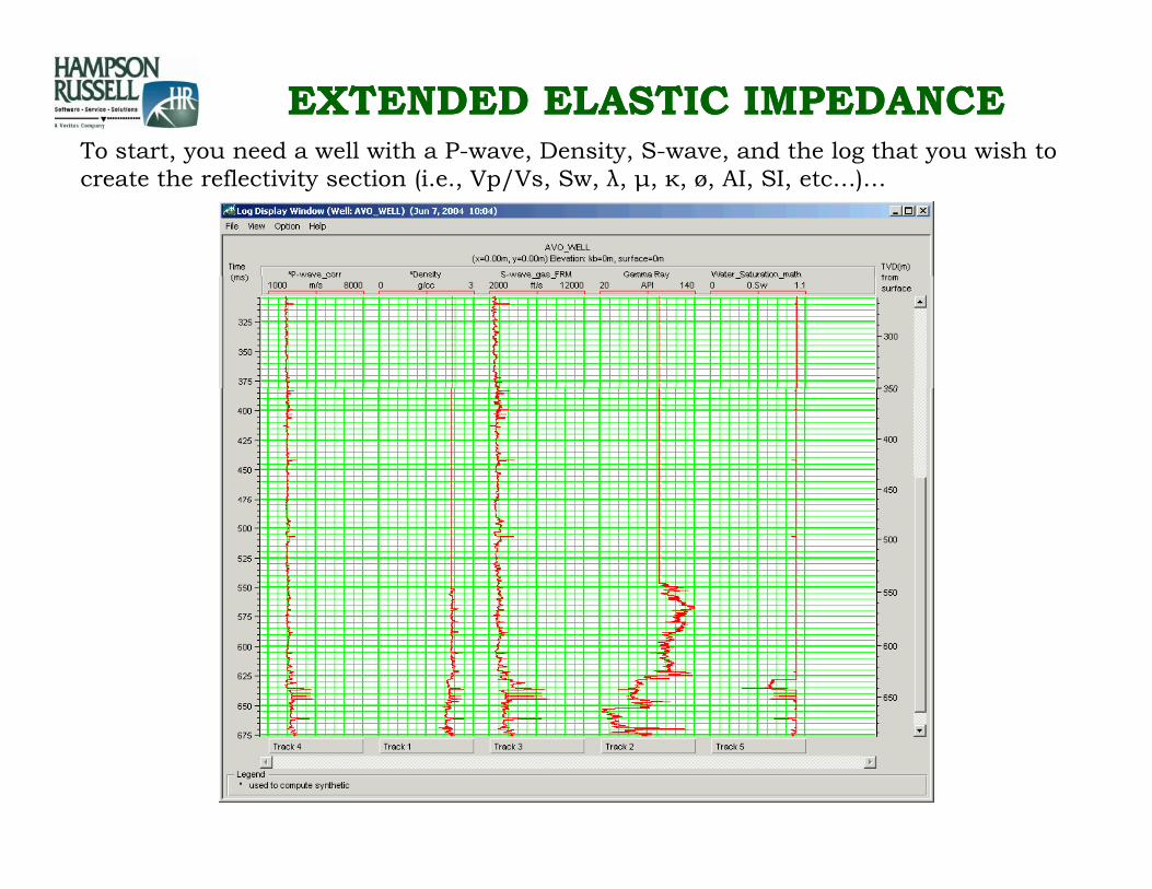
EXTENDED ELASTIC IMPEDANCEEXTENDED ELASTIC IMPEDANCETo start, you need a well with a P-wave, Density, S-wave, and the log that you wish to create the reflectivity section (i.e., Vp/Vs, Sw, λ, μ, κ, ø, AI, SI, etc…)…

EXTENDED ELASTIC IMPEDANCEEXTENDED ELASTIC IMPEDANCENow open the CE7 AVO version and build a 3D depth model using the Advanced Setup…

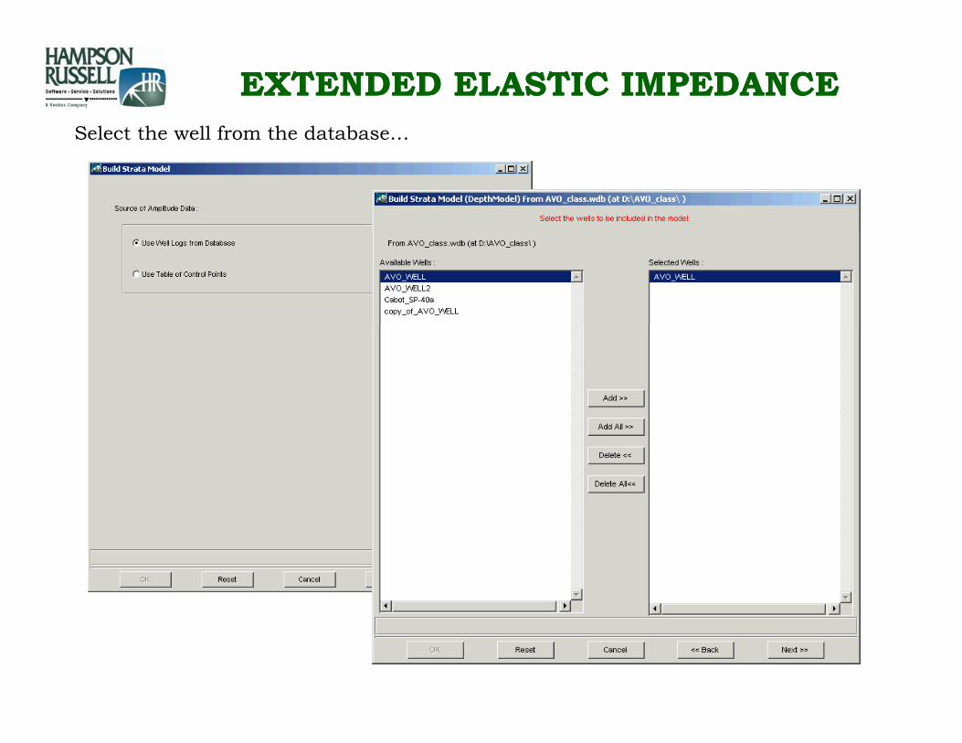
EXTENDED ELASTIC IMPEDANCEEXTENDED ELASTIC IMPEDANCESelect the well from the database…Select the well from the database…

EXTENDED ELASTIC IMPEDANCEEXTENDED ELASTIC IMPEDANCE…and build the geometry.

The first trick to making this process work is to have something in the header that can be related to angle. In this example, I have built a model with 181 traces that start from X = -90 to X = 90. The X value will now correspond to the angle…

EXTENDED ELASTIC IMPEDANCEEXTENDED ELASTIC IMPEDANCESelect the logs for the model: P-wave, Density, S-wave. The second trick is to also include the other logs that you wish to correlate with…


Make a note of the sample rate that you are using. In this case, my volume is sampled every 0.20 m…sampled every 0.20 m…

EXTENDED ELASTIC IMPEDANCEEXTENDED ELASTIC IMPEDANCEM th ll t th l ti di t 0º (i th A ti I d l ti )Map the well to the location corresponding to 0º (i.e., the Acoustic Impedance location)…

EXTENDED ELASTIC IMPEDANCEEXTENDED ELASTIC IMPEDANCENow apply a Trace Maths script to the P-wave, Density and S-wave log volumes to create the EEI log spectrum.

** Rename the volume variables to P_wave, Density and S_wave as shown…

EXTENDED ELASTIC IMPEDANCEEXTENDED ELASTIC IMPEDANCEY t t ll th You may want to call the output something useful like EEI_logs…


Load the EEI.prs file from the Trace Maths directory into the parser window.

If you made your X’s equal to your angles and if you renamed the volume variables, then you do not have to ychange anything in this script…

This script calculates the K This script calculates the K value for you. If you want to hard-code your K, edit this part here.

EXTENDED ELASTIC IMPEDANCEEXTENDED ELASTIC IMPEDANCEThe result is the spectrum of Elastic Impedance logs ranging form –90º to +90º. I have changed the Inserted Curve to the P-Impedance log for a comparison.

EXTENDED ELASTIC IMPEDANCEEXTENDED ELASTIC IMPEDANCEN th T M th i t t l t f th th l i th

Change the EEI logs volume variable name to ref and the other log volume to input and t th U f b th t d Ch th t t t thi f l lik

Now use another Trace Maths script to cross-correlate one of the other logs in the depth model against the EEI log suite. In my example, I will first cross-correlate the EEI logs with the Porosity log volume.

set the Usage of both to used. Change the output name to something useful like xcor_por to indicate that it is the cross-correlation of the porosity logs with the EEI logs...

EXTENDED ELASTIC IMPEDANCEEXTENDED ELASTIC IMPEDANCEThe Trace Maths script, crossCorrelateReflectivity, is referenced to the depths.

This is where you set your parameters In this example parameters. In this example, my sample rate, s_int, is 0.20 m. I am starting the correlation window at inputStartDepth = 550 m and inputStartDepth = 550 m and the window ends at inputEndDepth = 710 m. The cross-correlation coefficients are going to be output at are going to be output at outputStartDepth = 160 m depth in the output volume. I’ve set the delay (maxDelay) to 0 to just do a straight cross-to 0 to just do a straight cross-correlation…

EXTENDED ELASTIC IMPEDANCEEXTENDED ELASTIC IMPEDANCETh t t b bl ’t l k t i t ti Y ’ll h t h f th i The output probably won’t look to interesting. You’ll have to change some of the view parameters like the zoom, Mean and Std, turn off fill trace and color interpolation, etc…

EXTENDED ELASTIC IMPEDANCEEXTENDED ELASTIC IMPEDANCET t thi th t l k bit b ttTo get something that looks a bit better…

EXTENDED ELASTIC IMPEDANCEEXTENDED ELASTIC IMPEDANCENow cross-correlate the EEI logs with the some other logs. In this example, I’ll now Now cross correlate the EEI logs with the some other logs. In this example, I ll now cross-plot against a lithology indicator log like the Gamma Ray…

EXTENDED ELASTIC IMPEDANCEEXTENDED ELASTIC IMPEDANCETh fl ti it l l t d ith th EEI fl ti it lThe gamma ray reflectivity log cross-correlated with the EEI reflectivity logs.

EXTENDED ELASTIC IMPEDANCEEXTENDED ELASTIC IMPEDANCEIt’s probably best to view the cross-correlation results in a Cross-Plot display. Bring It s probably best to view the cross correlation results in a Cross Plot display. Bring both cross-correlation results into the cross-plot window…

EXTENDED ELASTIC IMPEDANCEEXTENDED ELASTIC IMPEDANCENow click on the New Plot > Primary Data to make a crossplot of the X-coord on the Now click on the New Plot > Primary Data to make a crossplot of the X coord on the X-axis and the cross-correlation results on the Y-axis.

EXTENDED ELASTIC IMPEDANCEEXTENDED ELASTIC IMPEDANCEThe cross-correlation of the Porosity reflectivity with the EEI reflectivity log spectrumThe cross correlation of the Porosity reflectivity with the EEI reflectivity log spectrum

A zoomed in view shows the maximum A zoomed in view shows the maximum negative correlation at 45º…

EXTENDED ELASTIC IMPEDANCEEXTENDED ELASTIC IMPEDANCEThe cross-correlation of the Gamma Ray reflectivity log with the EEI reflectivity log spectrum

A zoomed in view shows the maximum correlation at 65º…

EXTENDED ELASTIC IMPEDANCEEXTENDED ELASTIC IMPEDANCEHere, I cross-correlated the P-Impedance reflectivity log against the EEI reflectivity log Here, I cross correlated the P Impedance reflectivity log against the EEI reflectivity log spectrum. As expected, we get a perfect correlation at 0º …

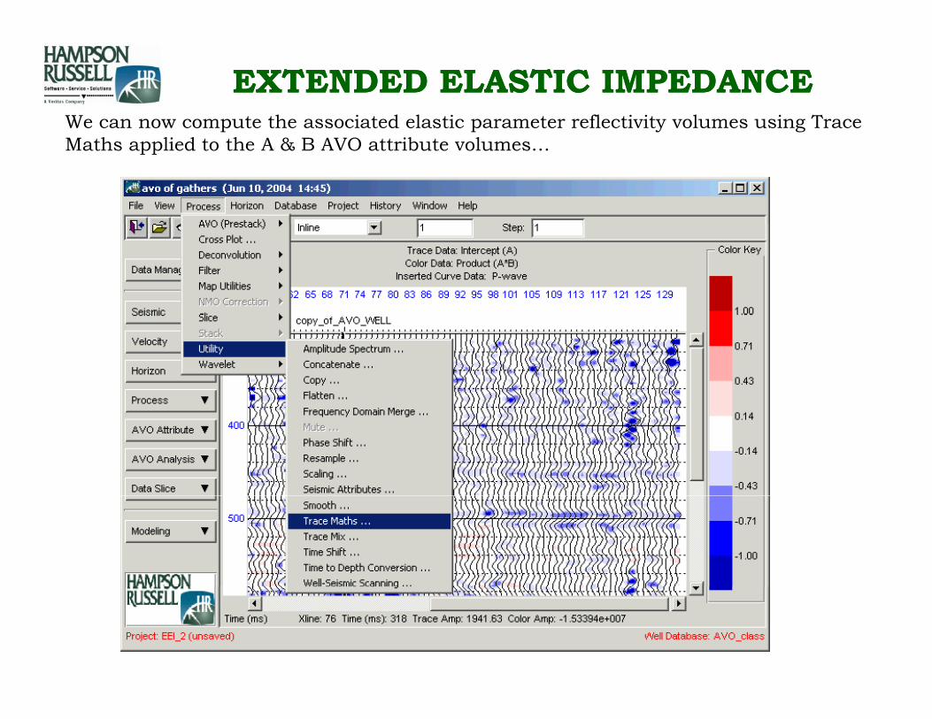
EXTENDED ELASTIC IMPEDANCEEXTENDED ELASTIC IMPEDANCEWe can now compute the associated elastic parameter reflectivity volumes using Trace Maths applied to the A & B AVO attribute volumes…

EXTENDED ELASTIC IMPEDANCEEXTENDED ELASTIC IMPEDANCET t th it fl ti it I’ d th AVO I t t d G di t To compute the porosity reflectivity, I’ve renamed the AVO Intercept and Gradient volume variables to A & B…

EXTENDED ELASTIC IMPEDANCEEXTENDED ELASTIC IMPEDANCEA d t i th ti And type in the equation: -1*( A + B*tan(45 * pi / 180) ). In this case, the maximum correlation was a negative value so I have negative value so I have negated the results…


The porosity reflectivity volume…

EXTENDED ELASTIC IMPEDANCEEXTENDED ELASTIC IMPEDANCEAs well, I’ll compute the lithology reflectivity…As well, I ll compute the lithology reflectivity…


The lithology reflectivity volumevolume…


In Strata we can invert these volumes to yield…

EXTENDED ELASTIC IMPEDANCEEXTENDED ELASTIC IMPEDANCEThe inverted porosity volumeThe inverted porosity volume

EXTENDED ELASTIC IMPEDANCEEXTENDED ELASTIC IMPEDANCEThe inverted lithology volumeThe inverted lithology volume

EXTENDED ELASTIC IMPEDANCEEXTENDED ELASTIC IMPEDANCEAnd an interpretation volume from the cross-plot.And an interpretation volume from the cross plot.

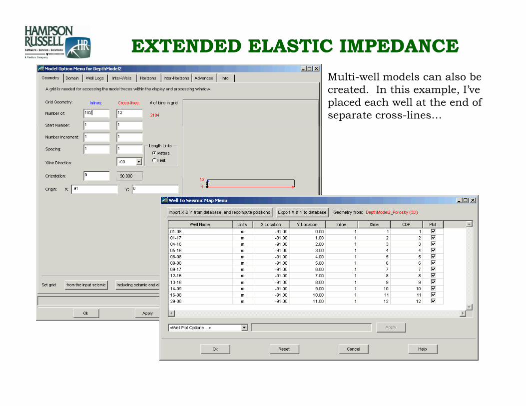
EXTENDED ELASTIC IMPEDANCEEXTENDED ELASTIC IMPEDANCEM lti ll d l l b Multi-well models can also be created. In this example, I’ve placed each well at the end of separate cross-lines…


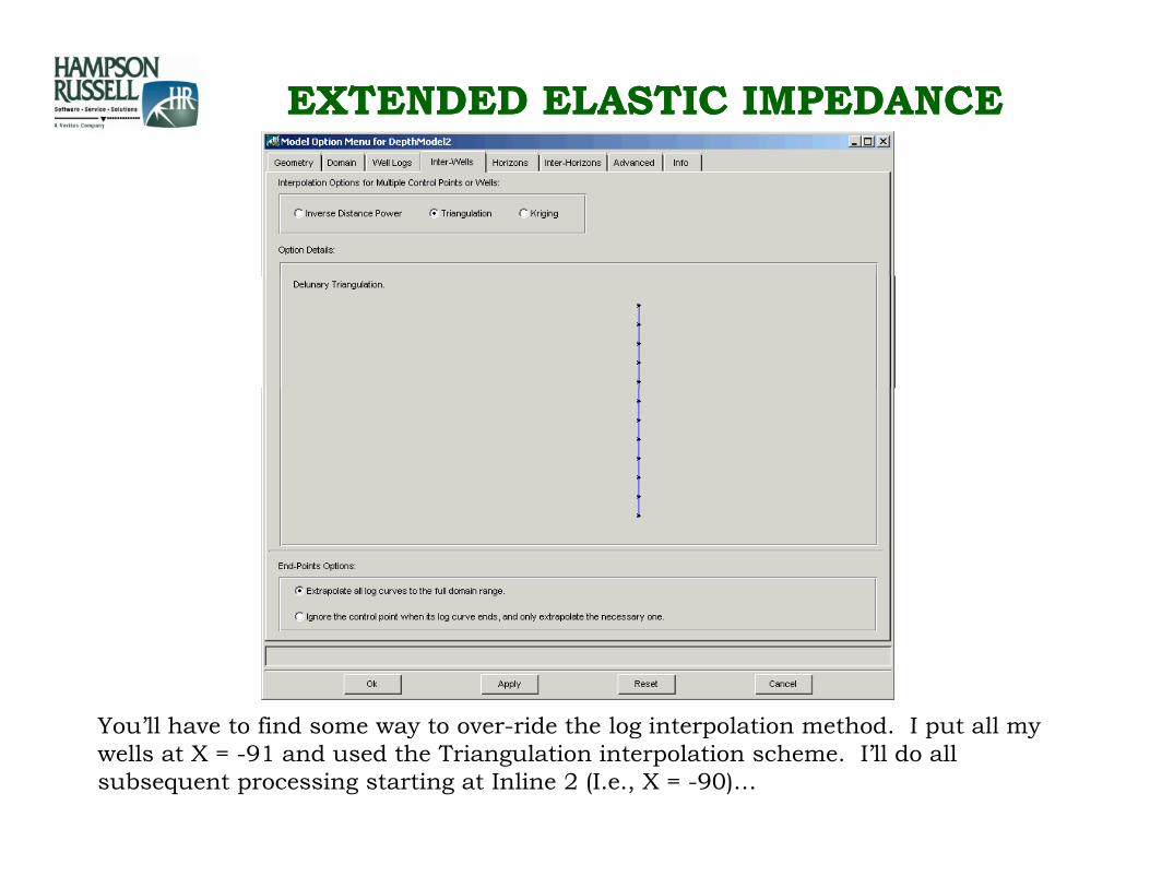
You’ll have to find some way to over ride the log interpolation method I put all my You ll have to find some way to over-ride the log interpolation method. I put all my wells at X = -91 and used the Triangulation interpolation scheme. I’ll do all subsequent processing starting at Inline 2 (I.e., X = -90)…

EXTENDED ELASTIC IMPEDANCEEXTENDED ELASTIC IMPEDANCEHere’s the cross-correlation of the porosity reflectivity for 12 wells against the EEI reflectivity log spectrum. It’s up to you to determine which cross-line corresponds to which Well. The Well in blue does not have a porosity log.

EXTENDED ELASTIC IMPEDANCEEXTENDED ELASTIC IMPEDANCEThe second method of EEI involves creating the scaled reflectivity trace spectrum The second method of EEI involves creating the scaled reflectivity trace spectrum volume from the AVO A & B attributes and cross-correlating them with the logs.

To test this method, I’ve created a synthetic gather and extracted the AVO attributes….


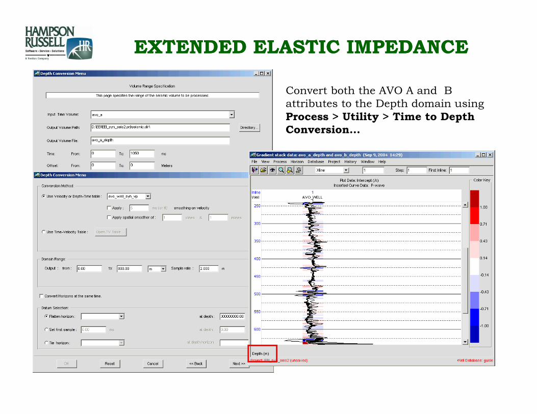
Convert both the AVO A and B attributes to the Depth domain using Process > Utility > Time to Depth ConversionConversion…

EXTENDED ELASTIC IMPEDANCEEXTENDED ELASTIC IMPEDANCEN b ild th d th d l i ll th l I’ Now build the depth model using all the logs. I’ve created a model with 182 traces starting from X = -91 to X = 90


Now we have to make the AVO A & B volumes the same size as the Depth Model. Use Process > Utility > Concatenate and copy the trace 181 times…


Here’s the new AVO A & B traces in depth copied 181 times.

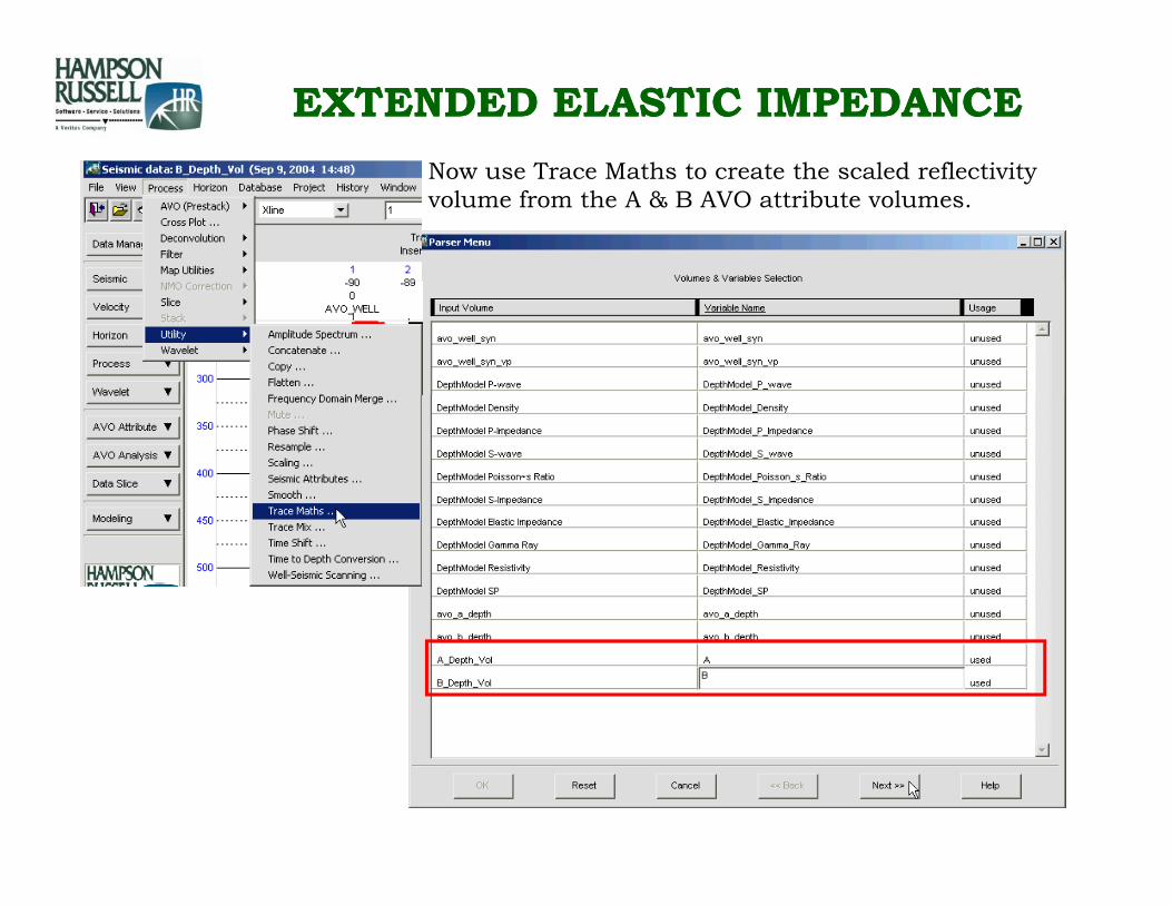
EXTENDED ELASTIC IMPEDANCEEXTENDED ELASTIC IMPEDANCEN T M th t t th l d fl ti it Now use Trace Maths to create the scaled reflectivity volume from the A & B AVO attribute volumes.


Call the output something useful – like scaled_reflectivity

And type in the script

rA = rad( inline - 91 );

output = A * cos( rA ) + B * sin( rA );

t tAnd type in the script.In this case, I refer the angle to the inline values…

output;

EXTENDED ELASTIC IMPEDANCEEXTENDED ELASTIC IMPEDANCETh l d fl ti it l h ld h f id t th th h th t The scaled_reflectivity volume should change from one side to the other such that troughs become peaks and vice versa…

EXTENDED ELASTIC IMPEDANCEEXTENDED ELASTIC IMPEDANCEAnother test to determine if the scaled_reflectivity was calculated correctly is to open the AVO A volume and view the difference between the two traces. The two should cancel each other out at 0 degrees…

EXTENDED ELASTIC IMPEDANCEEXTENDED ELASTIC IMPEDANCEN T M th t l t Now use Trace Maths to cross-correlate the scaled reflectivity with the target log. In my case, I will test this with the P-Impedance log curve…

For this particular script to work you should name the work, you should name the scaled reflectivity volume seismic and the target log volume should be called logs…


Call the output something useful…

and load in the following script: and load in the following script: crossCorrelateLogReflectivityWSeismic

EXTENDED ELASTIC IMPEDANCEEXTENDED ELASTIC IMPEDANCEThis script is similar to the s sc pt s s to t eother cross-correlation trace maths script – but it calculates the reflectivity of the logs volume and cross-

l t it ith th seismiccorrelates it with the seismicvolume – make sure that the logs volume is renamed as logs and that the scaled reflectivity volume is renamed yas seismic.

Again, only edit the values in the USER-DEFINED PARAMETERS section.

EXTENDED ELASTIC IMPEDANCEEXTENDED ELASTIC IMPEDANCECross-plot the resulting cross-correlation volume against itself and adjust the plot parameters to plot the X-Coord on the X-axis. As expected, we see the greatest positive correlation at nearly 0 degrees.

EXTENDED ELASTIC IMPEDANCEEXTENDED ELASTIC IMPEDANCEThis approach can probably be applied to multiple wells in a seismic volume. I will not demonstrate this whole process – because I don’t have an appropriate data set.

First extract an arbitrary line on the AVO attribute volume that goes through all the wells and only extracts at the node pointswells and only extracts at the node points…

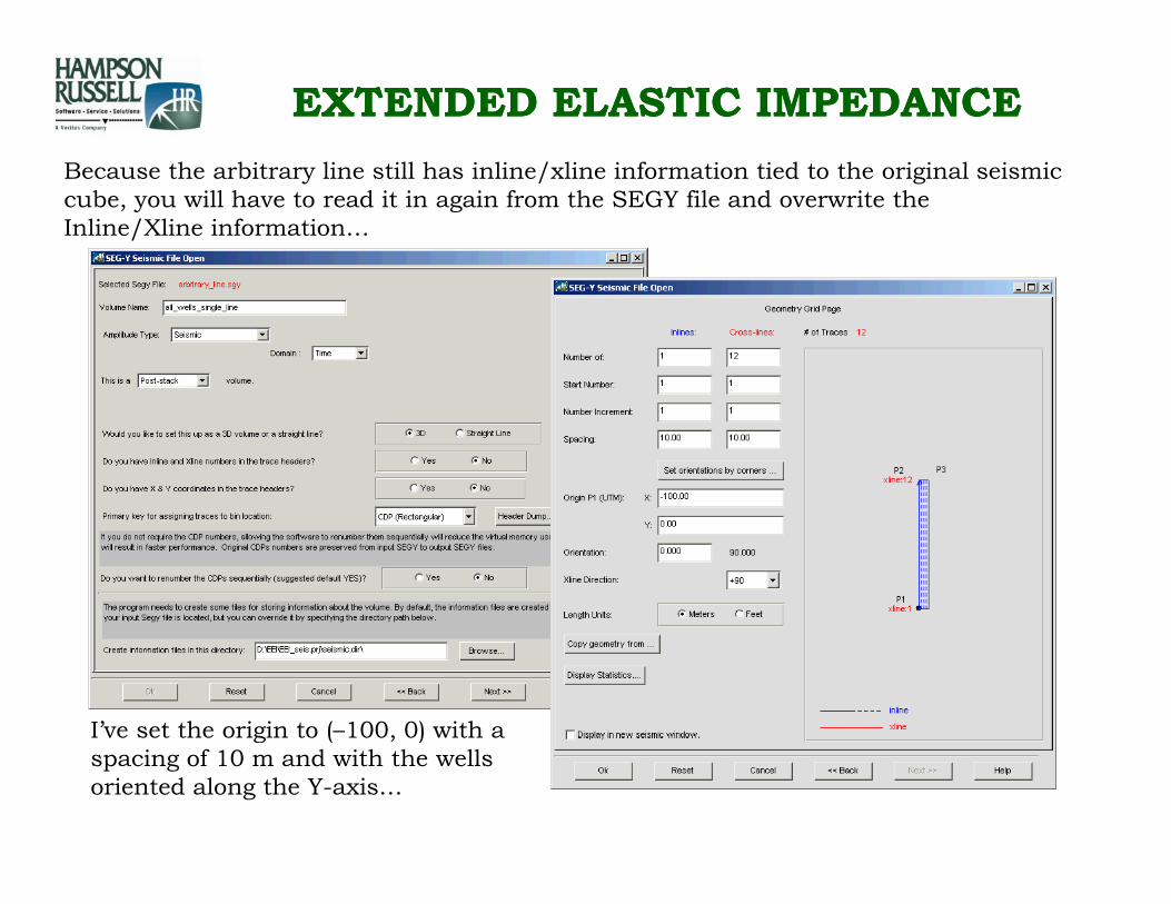
EXTENDED ELASTIC IMPEDANCEEXTENDED ELASTIC IMPEDANCEB th bit li till h i li / li i f ti ti d t th i i l i i Because the arbitrary line still has inline/xline information tied to the original seismic cube, you will have to read it in again from the SEGY file and overwrite the Inline/Xline information…

I’ve set the origin to (–100, 0) with a I ve set the origin to ( 100, 0) with a spacing of 10 m and with the wells oriented along the Y-axis…


Next, I’ll use the concatenation process to repeat the inline 181 times to create a range of times to create a range of χ’s from –91 to +90…

EXTENDED ELASTIC IMPEDANCEEXTENDED ELASTIC IMPEDANCEI’ll th ll t th fi t i li t X 100 I’ll remap the wells to the first inline at X = -100 …

EXTENDED ELASTIC IMPEDANCEEXTENDED ELASTIC IMPEDANCEAnd build the log model volume. Then apply the cross-correlation script as before.And build the log model volume. Then apply the cross correlation script as before.

EXTENDED ELASTIC IMPEDANCEEXTENDED ELASTIC IMPEDANCEACKNOWLEDGEMENTSACKNOWLEDGEMENTS

Thanks to

• Dan Hampson (HRS) for suggesting cross-correlating the log reflectivities.

• Richard Kruger (BP, Calgary) for suggesting creating the scaled reflectivity volume and cross-correlating with the logs.

• Brian Russell (HRS) and John Logel (Anadarko, Calgary) for their comments and suggestionsand suggestions.

Extended Elastic Impedance.ppt - CGG€¦ · we can implement both methods of the Extended Elastic...

Documents

Transcript of Extended Elastic Impedance.ppt - CGG€¦ · we can implement both methods of the Extended Elastic...