Expressing Combinatorial Optimization Problems …Expressing Combinatorial Optimization Problems by...
29
Expressing Combinatorial Optimization Problems by Systems of Polynomial Equations and the Nullstellensatz J.A. DE LOERA 1† , J. LEE 2 , S. MARGULIES 3† and S. ONN 4‡ 1 Department of Mathematics, Univ. of California, Davis, California, USA (email: [email protected]) 2 IBM T.J. Watson Research Center, Yorktown Heights, New York, USA (email: [email protected]) 3 Department of Computer Science, Univ. of California, Davis, California, USA (email: [email protected]) 4 Davidson Faculty of IE & M, Technion - Israel Institute of Technology, Haifa, Israel (email: [email protected]) Systems of polynomial equations over the complex or real numbers can be used to model combinatorial problems. In this way, a combinatorial problem is feasible (e.g. a graph is 3-colorable, hamiltonian, etc.) if and only if a related system of polynomial equations has a solution. In the first part of this paper, we construct new polynomial encodings for the problems of finding in a graph its longest cycle, the largest planar subgraph, the edge-chromatic number, or the largest k-colorable subgraph. For an infeasible polynomial system, the (complex) Hilbert Nullstellensatz gives a certificate that the associated combinatorial problem is infeasible. Thus, unless P = NP , there must exist an infinite sequence of infeasible instances of each hard combinatorial problem for which the minimum degree of a Hilbert Nullstellensatz certificate of the associated polynomial system grows. We show that the minimum-degree of a Nullstellensatz certificate for the non-existence of a stable set of size greater than the stability number of the graph is the stability number of the graph. Moreover, such a certificate contains at least one term per stable set of G . In contrast, for non-3-colorability, we found only graphs with Nullstellensatz certificates of degree four. 1. Introduction N. Alon [1] used the term “polynomial method” to refer to the use of non-linear polynomials for solving combinatorial problems. Although the polynomial method is not yet as widely used by combinatorists as, for instance, polyhedral or probabilistic techniques, the literature in this subject continues to grow. Prior work on encoding combinatorial properties included colorings [2, 9, 10, 15, 24, 27, 28, 29], stable sets [9, 23, 24, 36], matchings [11], and flows [2, 29, 30]. Non-linear encodings of combinatorial problems are often compact. This contrasts with the exponential sizes of systems of linear inequalities that describe the convex hull of incidence vectors of many combinatorial structures (see [37]). In this article we present new encodings for other combinatorial problems, and we discuss applications of polynomial encodings to combinatorial optimization and to computational complexity. † Research supported in part by an IBM Open Collaborative Research Award and by NSF grant DMS-0608785 ‡ Research supported by the ISF (Israel Science Foundation) and by the fund for the promotion of research at Technion arXiv:0706.0578v1 [math.CO] 5 Jun 2007
Transcript of Expressing Combinatorial Optimization Problems …Expressing Combinatorial Optimization Problems by...

Expressing Combinatorial Optimization Problems bySystems of Polynomial Equations and the
Nullstellensatz
J . A . D E L O E R A1†, J . L E E2, S . M A R G U L I E S3† and S . O N N4‡
1 Department of Mathematics, Univ. of California, Davis, California, USA
(email: [email protected])
2 IBM T.J. Watson Research Center, Yorktown Heights, New York, USA
(email: [email protected])
3 Department of Computer Science, Univ. of California, Davis, California, USA
(email: [email protected])
4Davidson Faculty of IE & M, Technion - Israel Institute of Technology, Haifa, Israel
(email: [email protected])
Systems of polynomial equations over the complex or real numbers can be used to model combinatorial
problems. In this way, a combinatorial problem is feasible (e.g. a graph is 3-colorable, hamiltonian, etc.)if and only if a related system of polynomial equations has a solution. In the first part of this paper, we
construct new polynomial encodings for the problems of finding in a graph its longest cycle, the largest
planar subgraph, the edge-chromatic number, or the largest k-colorable subgraph.
For an infeasible polynomial system, the (complex) Hilbert Nullstellensatz gives a certificate that the
associated combinatorial problem is infeasible. Thus, unless P = NP , there must exist an infinite sequenceof infeasible instances of each hard combinatorial problem for which the minimum degree of a Hilbert
Nullstellensatz certificate of the associated polynomial system grows.
We show that the minimum-degree of a Nullstellensatz certificate for the non-existence of a stable set ofsize greater than the stability number of the graph is the stability number of the graph. Moreover, such a
certificate contains at least one term per stable set of G . In contrast, for non-3-colorability, we found only
graphs with Nullstellensatz certificates of degree four.
1. Introduction
N. Alon [1] used the term “polynomial method” to refer to the use of non-linear polynomials for solvingcombinatorial problems. Although the polynomial method is not yet as widely used by combinatorists as, forinstance, polyhedral or probabilistic techniques, the literature in this subject continues to grow. Prior work onencoding combinatorial properties included colorings [2, 9, 10, 15, 24, 27, 28, 29], stable sets [9, 23, 24, 36],matchings [11], and flows [2, 29, 30]. Non-linear encodings of combinatorial problems are often compact.This contrasts with the exponential sizes of systems of linear inequalities that describe the convex hullof incidence vectors of many combinatorial structures (see [37]). In this article we present new encodingsfor other combinatorial problems, and we discuss applications of polynomial encodings to combinatorialoptimization and to computational complexity.
† Research supported in part by an IBM Open Collaborative Research Award and by NSF grant DMS-0608785‡ Research supported by the ISF (Israel Science Foundation) and by the fund for the promotion of research at Technion
arX
iv:0
706.
0578
v1 [
mat
h.C
O]
5 J
un 2
007
2 J.A. De Loera, J. Lee, S. Margulies, S. Onn
Recent work demonstrates that one can derive good semidefinite programming relaxations for combina-torial optimization problems from the encodings of these problems as polynomial systems (see [22] andreferences therein for details). Lasserre [20], Laurent [21] and Parrilo [31, 32] studied the problem of min-imizing a general polynomial function f(x) over an algebraic variety having only finitely many solutions.Laurent proved that when the variety consists of the solutions of a zero-dimensional radical ideal I , thereis a way to set up the optimization problem minf(x) : x ∈ variety(I) as a finite sequence of semidefiniteprograms terminating with the optimal solution (see [21]).
This immediately suggests an application of the polynomial method to combinatorial optimization prob-lems: Encode your problem with polynomials equations in R[x1, . . . , xn] that generate a zero-dimensional(variety is finite) radical ideal, then generate the finite sequence of SDPs following the method in [21]. Thishighlights the importance of finding systems of polynomials for various combinatorial optimization prob-lems. The first half of this paper proposes new polynomial system encodings for the problems, with respectto an input graph, of finding a longest cycle, a largest planar subgraph, a largest k-colorable subgraph, or aminimum edge coloring. In particular, we establish the following result.
Theorem 1.1.
1. A simple graph G with nodes 1, . . . , n has a cycle of length L if and only if the following zero-dimensionalsystem of polynomial equations has a solution:
n∑i=1
yi = L . (1.1)
For every node i = 1, . . . , n:
yi(yi − 1) = 0,n∏s=1
(xi − s) = 0 , (1.2)
yi∏
j∈Adj(i)(xi − yjxj + yj)(xi − yjxj − yj(L− 1)) = 0 . (1.3)
Here Adj(i) denotes the set of nodes adjacent to node i .2. Let G be a simple graph with n nodes and m edges. G has a planar subgraph with K edges if and only if
the following zero-dimensional system of equations has a solution:For every edge i, j ∈ E(G):
z2ij − zij = 0,
∑i,j∈E(G)
zij −K = 0 . (1.4)
For k = 1, 2, 3 , every node i ∈ V (G) and every edge i, j ∈ E(G):
n+m∏s=1
(xik − s) = 0,n+m∏s=1
(yijk − s) = 0 , (1.5)
sk
∏i,j∈V (G)i<j
(xik − xjk
) ∏i∈V (G),
u,v∈E(G)
(xik − yuvk
) ∏i,j,u,v∈E(G)
(yijk − yuvk
) = 1 . (1.6)
For k = 1, 2, 3 , and for every pair of a node i ∈ V (G) and incident edge i, j ∈ E(G):
zij(yijk − xik −∆ij,ik
)= 0 . (1.7)

Expressing Combinatorial Problems by Polynomial Equations 3
For every pair of a node i ∈ V (G) and edge u, v ∈ E(G) that is not incident on i:
zuv(yuv1 − xi1 −∆uv,i1
)(yuv2 − xi2 −∆uv,i2
)(yuv3 − xi3 −∆uv,i3
)= 0 , (1.8)
zuv(xi1 − yuv1 −∆i,uv1
)(xi2 − yuv2 −∆i,uv2
)(xi3 − yuv3 −∆i,uv3
)= 0 . (1.9)
For every pair of edges i, j, u, v ∈ E(G) (regardless of whether or not they share an endpoint):
zijzuv(yij1−yuv1−∆ij,uv1
)(yij2−yuv2−∆ij,uv2
)(yij3−yuv3−∆ij,uv3
)= 0 , (1.10)
zijzuv(yuv1−yij1−∆uv,ij1
)(yuv2−yij2−∆uv,ij2
)(yuv3−yij3−∆uv,ij3
)= 0 . (1.11)
For every pair of nodes i, j ∈ V (G) , (regardless of whether or not they are adjacent):(xi1 − xj1 −∆i,j1
)(xi2 − xj2 −∆i,j2
)(xi3 − xj3 −∆i,j3
)= 0 , (1.12)(
xj1 − xi1 −∆j,i1)(xj2 − xi2 −∆j,i2
)(xj3 − xi3 −∆j,i3
)= 0 . (1.13)
For every ∆index (e.g., ∆ij,uvk,∆ij,ik , etc.) variable appearing in the above system:
n+m−1∏d=1
(∆index − d
)= 0 . (1.14)
3. A graph G has a k-colorable subgraph with R edges if and only if the following zero-dimensional systemof equations has a solution: ∑
i,j∈E(G)
yij −R = 0 . (1.15)
For every vertex i ∈ V (G):
xki = 1 . (1.16)
For every edge i, j ∈ E(G):
y2ij − yij = 0, yij
(xk−1i + xk−2
i xj + · · ·+ xk−1j
)= 0 . (1.17)
4. Let G be a simple graph with maximum vertex degree ∆ . The graph G has edge-chromatic number ∆ ifand only if the following zero-dimensional system of polynomials has a solution:For every edge i, j ∈ E(G):
x∆ij = 1 . (1.18)
For every node i ∈ V (G):
si
∏j,k∈Adj(i)j<k
(xij − xik)
= 1 , (1.19)
where Adj(i) is the set of nodes adjacent to node i .[By Vizing’s theorem, if the system has no solution, then G has edge-chromatic number ∆ + 1 .]
In the second half of the article, we look at the connection between polynomial systems and computationalcomplexity. We have already mentioned that semidefinite programming is one way to approach optimization.It is natural to ask how big are such SDPs. For simplicity of analysis, we look at the case of feasibility insteadof optimization. In this case, the SDPs are replaced by a large-scale linear algebra problem. We will discussdetails in Section 3. For a hard optimization problem, say Max-Cut, we associate a system of polynomialequations J such that the system has a solution if and only if the problem has a feasible solution. Onthe other hand, the famous Hilbert Nullstellensatz (see [7]) states that a system of polynomial equations

4 J.A. De Loera, J. Lee, S. Margulies, S. Onn
J = f1(x) = 0, f2(x) = 0, . . . , fr(x) = 0 with complex coefficients has no solution in Cn if and only if thereexist polynomials α1, . . . , αr ∈ C[x1, . . . , xn] such that 1 =
∑αifi . Thus, if the polynomial system J has
no solution, there exists a certificate that the combinatorial optimization problem is infeasible.
There are well-known upper bounds for the degrees of the coefficients αi in the Hilbert Nullstellensatzcertificate for general systems of polynomials, and they turn out to be sharp (see [18]). For instance, thefollowing well-known example shows that the degree of α1 is at least dm :
f1 = xd1, f2 = x1 − xd2, . . . , fm−1 = xm−2 − xdm−1, fm = 1− xm−1xd−1m .
But polynomial systems for combinatorial optimization are special. One question is how complicated arethe degrees of Nullstellensatz certificates of infeasibility? As we will see in Section 3, unless P = NP , forevery hard combinatorial problem, there must exist an infinite sequence of infeasible instances for which theminimum degree of a Nullstellensatz certificate, for the associated system of polynomials, grows arbitrarilylarge. This was first observed by L. Lovasz who proposed the problem of finding explicit graphs in [24]. Amain contribution of this article is to exhibit such growth of degree explicitly. In the second part of the paperwe discuss the growth of degree for the NP-complete problems stable set and 3-colorability. We establish thefollowing theorem:
Theorem 1.2.
1. Given a graph G , let α(G) denote its stability number. A minimum-degree Nullstellensatz certificate forthe non-existence of a stable set of size greater than α(G) has degree equal to α(G) and contains at leastone term per stable set in G .
2. Every Nullstellensatz certificate for non-3-colorability of a graph has degree at least four. Moreover, inthe case of a graph containing an odd-wheel or a clique as a subgraph, a minimum-degree Nullstellensatzcertificate for non-3-colorability has degree exactly four.
The paper is organized as follows. Our encoding results for longest cycle and largest planar subgraphappear in Subsection 2.1. As a direct consequence, we recover a polynomial system characterization of thehamiltonian cycle problem. Similarly, we discuss how to express, in terms of polynomials, the decision questionof whether a poset has dimension p . The encodings for edge-chromatic number and largest k-colorablesubgraph also appear in Subsection 2.1. As we mentioned earlier, colorability problems were among the firststudied using the polynomial method; we revisit those earlier results and end Subsection 2.2 by proposing anotion of dual coloring derived from our algebraic set up. In Section 3 we discuss how the growth of degreein the Nullstellensatz occurs under the assumption P 6= NP . We also sketch a linear algebra procedurewe used to compute minimum-degree Nullstellensatz certificates for particular graphs. In Subsection 3.1we demonstrate the degree growth of Nullstellensatz certificates for the stable set problem. In contrast, inSubsection 3.2, we exhibit many non-3-colorable graphs where there is no growth of degree.
2. Encodings
In this section, we focus on how to find new polynomial encodings of some combinatorial optimizationproblems. We begin by recalling two nice results in the polynomial method that will be used later on. D.Bayer established a characterization of 3-colorability via a system of polynomial equations [4]. We generalizeBayer’s result as follows:
Lemma 2.1. The graph G is k-colorable if and only if the following zero-dimensional system of equations
xki − 1 = 0, for every node i ∈ V (G),xk−1i + xk−2
i xj + · · ·+ xk−1j = 0, for every edge i, j ∈ E(G) ,

Expressing Combinatorial Problems by Polynomial Equations 5
has a solution. Moreover, the number of solutions equals the number of distinct k-colorings multiplied by k! .
Recall that a stable set or independent set in a graph G is a subset of vertices such that no two verticesin the subset are adjacent. The maximum size α(G) of a stable set is called the stability number of G . Weview the stable sets in terms of their incidence vectors. These are 0/1 vectors of length |V | , one for everystable set, where a one in the i-th entry indicates that the i-th vertex is a member of the associated stableset. These 0/1 vectors can be fully described by a small system of quadratic equations:
Lemma 2.2 (L. Lovasz [24]). The graph G has stability number at least k if and only if the followingzero-dimensional system of equations
x2i − xi = 0, for every node i ∈ V (G), (2.1)
xixj = 0, for every edge i, j ∈ E(G), (2.2)n∑i=1
xi = k, (2.3)
has a solution.
Example 2.3. Consider the Petersen graph labeled as in Figure 1. If we wish to check whether there are
Figure 1.Petersen graph
stable sets of size four, we take the ideal I generated by the polynomials in Eq. 2.1, 2.2 and 2.3:
I =⟨x2
1 − x1, x22 − x2, x
23 − x3, x
24 − x4, x
25 − x5, x
26 − x6, x
27 − x7, x
28 − x8, x
29 − x9, x
210 − x10,
x1x6, x2x8, x3x10, x4x7, x5x9, x1x2, x2x3, x3x4, x4x5, x1x5, x6x7, x7x8, x8x9, x9x10, x6x10,
x1 + x2 + x3 + x4 + x5 + x6 + x7 + x8 + x9 + x10 − 4⟩.
By construction, we know that the quotient ring R := C[x1, . . . , x10]/I is a finite-dimensional C-vectorspace. Because the ideal I is radical, its dimension equals the number of stable sets of cardinality four inthe Petersen graph (not taking symmetries into account). Using Grobner bases, we find that the monomials1, x10, x9, x8, x7 form a vector-space basis of R and that there are no solutions with cardinality five; thusα(Petersen) = 4 . It is important to stress that we can recover the five different maximum-cardinality stablesets from the knowledge of the complex finite-dimensional vector space basis of R (see [8]).
Next we establish similar encodings for the combinatorial problems stated in Theorem 1.1.
2.1. Proof of Theorem 1.1
Proof (Theorem 1.1, Part 1). Suppose that a cycle C of length L exists in the graph G . We set yi = 1or 0 depending on whether node i is on C or not. Next, starting the numbering at any node of C , we setxi = j if node i is the j-th node of C . It is easy to check that Eqs. 1.1 and 1.2 are satisfied.
To verify Eq. 1.3, note that since C has length L , if vertex i is the j-th node of the cycle, then one of its
6 J.A. De Loera, J. Lee, S. Margulies, S. Onn
neighbors, say k , must be the “follower”, namely the (j + 1)-th element of the cycle. If j < L , then thefactor (xi − xk − 1) = 0 appears in the product equation associated with the i-th vertex, and the product iszero. If j = L , then the factor (xi−xk − (L− 1)) = 0 appears, and the product is again 0. Since this is truefor all vertices that are turned “on”, and for all vertices that are “off”, we have Eq. 1.3 automatically equalto zero, all of the equations of the polynomials vanish.
Conversely, from a solution of the system above, we see that L variables yi are not zero; call this set C .We claim that the nodes i ∈ C must form a cycle. Since yi 6= 0 , the polynomial of Eq. 1.3 must vanish; thusfor some j ∈ C ,
(xi − xj + 1) = 0 , or (xi − xj − (L− 1)) = 0 .
Note that Eq. 1.3 reduces to this form when yi = 1 . Therefore, either vertex i is adjacent to a vertex j (withyj = 1) such that xj equals the next integer value (xi + 1 = xj), or xi − L = xj − 1 (again, with yj = 1).In the second case, since xi and xj are integers between 1 and L , this forces xi = L and xj = 1 . By thepigeonhole principle, this implies that all integer values from 1 to L must be assigned to some node in C
starting at vertex 1 and ending at L (which is adjacent to the node receiving 1).
We have the following corollary.
Corollary 2.4. A graph G has a hamiltonian cycle if and only if the following zero-dimensional system of2n equations has a solution. For every node i ∈ V (G) , we have two equations:
n∏s=1
(xi − s) = 0 , and∏
j∈Adj(i)
(xi − xj + 1)(xi − xj − (n− 1)) = 0 .
The number of hamiltonian cycles in the graph G equals the number of solutions of the system divided by2n .
Proof. Clearly when L = n we can just fix all yi to 1 , thus many of the equations simplify or becomeobsolete. We only have to check the last statement on the number of hamiltonian cycles. For that, we remarkthat no solution appears with multiplicity because the ideal is radical. That the ideal is radical is implied bythe fact that every variable appears as the only variable in a unique square-free polynomial (see page 246 of[19]). Finally, note for every cycle there are n ways to choose the initial node to be labeled as 1 , and thentwo possible directions to continue the labeling.
Note that similar results can be established for the directed graph version, thus one can consider pathsor cycles with orientation. Also note that, we can use the polynomials systems above to investigate thedistribution of cycle lengths in a graph (similarly for path lengths and cut sizes). This topic has severaloutstanding questions. For example, a still unresolved question of Erdos and Gyarfas [35] asks: If G is agraph with minimum-degree three, is it true that G always has a cycle having length that is a power of two?Define the cycle-length polynomial as the square-free univariate polynomial whose roots are the possiblecycle lengths of a graph (same can be done for cuts). Considering L as a variable, the reduced lexicographicGrobner basis (with L the last variable) computation provides us with a unique univariate polynomial on Lthat is divisible by the cycle-length polynomial of G .
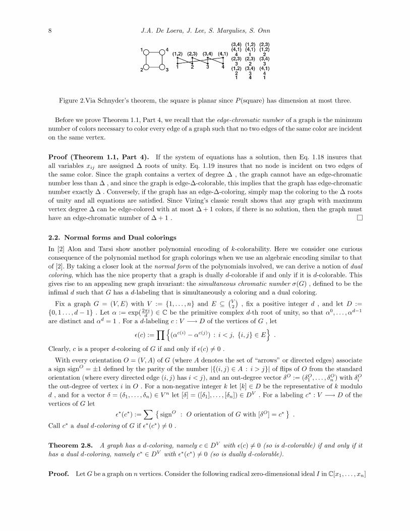
Now we proceed to the proof of part 2 of Theorem 1.1. For this we recall Schnyder’s characterization ofplanarity in terms of the dimension of a poset [33]: For an n-element poset P , a linear extension is an orderpreserving bijection σ : P → 1, 2, . . . , n . The poset dimension of P is the smallest integer t for which thereexists a family of t linear extensions σ1, . . . , σt of P such that x < y in P if and only if σi(x) < σi(y) for allσi . The incidence poset P (G) of a graph G with node set V and edge set E is the partially ordered set of

Expressing Combinatorial Problems by Polynomial Equations 7
height two on the union of nodes and edges, where we say x < y if x is a node and y is an edge, and y isincident to x .
Lemma 2.5 (Schnyder’s theorem [33]). A graph G is planar if and only if the poset dimension of P (G)is no more than three.
Thus our first step is to encode the linear extensions and the poset dimension of a poset P in terms ofpolynomial equations. The idea is similar to our characterization of cycles via permutations.
Lemma 2.6. The poset P = (E,>) has poset dimension at most p if and only if the following system ofequations has a solution:
For k = 1, . . . , p :
|E|∏s=1
(xi(k)− s) = 0, for every i ∈ 1, . . . , |E|, and sk
( ∏i,j∈1,...,|E|,
i<j
xi(k)− xj(k))
= 1 . (2.4)
For k = 1, . . . , p , and every ordered pair of comparable elements ei > ej in P :
xi(k)− xj(k)−∆ij(k) = 0. (2.5)
For every ordered pair of incomparable elements of P (i.e., ei 6> ej and ej 6> ei) :
p∏k=1
(xi(k)− xj(k)−∆ij(k)
)= 0 ,
p∏k=1
(xj(k)− xi(k)−∆ji(k)
)= 0 , (2.6)
For k = 1, . . . , p , and for every pair i, j ∈ 1, . . . , |E|:
|E|−1∏d=1
(∆ij(k)− d) = 0,|E|−1∏d=1
(∆ji(k)− d) = 0 . (2.7)
Proof. With Eqs. 2.4 and 2.5, we assign distinct numbers 1 through |E| to the poset elements, such thatthe properties of a linear extension are satisfied. Eqs. 2.4 and 2.5 are repeated p times, so p linear extensionsare created. If the intersection of these extensions is indeed equal to the original poset P , then for everyincomparable pair of elements in P , at least one of the p linear extensions must detect the incomparability.But this is indeed the case for Eq. 2.6, which says that for the l-th linear extension, the values assigned tothe incomparable pair ei, ej do not satisfy xi(l) < xj(l) , but instead satisfy xj(l) > xi(l) .
Proof (Theorem 1.1, Part 2). We simply apply the above lemma to the particular pairs of order relationsof the incidence poset of the graph. Note that in the formulation we added variables zij that have the effectof turning on or off an edge of the input graph.
Example 2.7 (Posets and Planar Graphs).
Proof (Theorem 1.1, Part 3). Using Lemma 2.1, we can finish the proof of Part 3. For a k-colorablesubgraph H of size R , we set yij = 1 if edge i, j ∈ E(H) or yij = 0 otherwise. By Lemma 2.1, the resultingsubsystem of equations has a solution. Conversely from a solution, the subgraph H in question is read offfrom those yij 6= 0 . Solvability implies that H is k-colorable.
8 J.A. De Loera, J. Lee, S. Margulies, S. Onn
Figure 2.Via Schnyder’s theorem, the square is planar since P (square) has dimension at most three.
Before we prove Theorem 1.1, Part 4, we recall that the edge-chromatic number of a graph is the minimumnumber of colors necessary to color every edge of a graph such that no two edges of the same color are incidenton the same vertex.
Proof (Theorem 1.1, Part 4). If the system of equations has a solution, then Eq. 1.18 insures thatall variables xij are assigned ∆ roots of unity. Eq. 1.19 insures that no node is incident on two edges ofthe same color. Since the graph contains a vertex of degree ∆ , the graph cannot have an edge-chromaticnumber less than ∆ , and since the graph is edge-∆-colorable, this implies that the graph has edge-chromaticnumber exactly ∆ . Conversely, if the graph has an edge-∆-coloring, simply map the coloring to the ∆ rootsof unity and all equations are satisfied. Since Vizing’s classic result shows that any graph with maximumvertex degree ∆ can be edge-colored with at most ∆ + 1 colors, if there is no solution, then the graph musthave an edge-chromatic number of ∆ + 1 .
2.2. Normal forms and Dual colorings
In [2] Alon and Tarsi show another polynomial encoding of k-colorability. Here we consider one curiousconsequence of the polynomial method for graph colorings when we use an algebraic encoding similar to thatof [2]. By taking a closer look at the normal form of the polynomials involved, we can derive a notion of dualcoloring, which has the nice property that a graph is dually d-colorable if and only if it is d-colorable. Thisgives rise to an appealing new graph invariant: the simultaneous chromatic number σ(G) , defined to be theinfimal d such that G has a d-labeling that is simultaneously a coloring and a dual coloring.
Fix a graph G = (V,E) with V := 1, . . . , n and E ⊆(V2
), fix a positive integer d , and let D :=
0, 1 . . . , d − 1 . Let α := exp( 2πid ) ∈ C be the primitive complex d-th root of unity, so that α0, . . . , αd−1
are distinct and αd = 1 . For a d-labeling c : V −→ D of the vertices of G , let
ε(c) :=∏
(αc(i) − αc(j)) : i < j, i, j ∈ E.
Clearly, c is a proper d-coloring of G if and only if ε(c) 6= 0 .
With every orientation O = (V,A) of G (where A denotes the set of “arrows” or directed edges) associatea sign signO = ±1 defined by the parity of the number |(i, j) ∈ A : i > j| of flips of O from the standardorientation (where every directed edge (i, j) has i < j), and an out-degree vector δO := (δO1 , . . . , δ
On ) with δOi
the out-degree of vertex i in O . For a non-negative integer k let [k] ∈ D be the representative of k modulod , and for a vector δ = (δ1, . . . , δn) ∈ V n let [δ] = ([δ1], . . . , [δn]) ∈ DV . For a labeling c∗ : V −→ D of thevertices of G let
ε∗(c∗) :=∑
signO : O orientation of G with [δO] = c∗.
Call c∗ a dual d-coloring of G if ε∗(c∗) 6= 0 .
Theorem 2.8. A graph has a d-coloring, namely c ∈ DV with ε(c) 6= 0 (so is d-colorable) if and only if ithas a dual d-coloring, namely c∗ ∈ DV with ε∗(c∗) 6= 0 (so is dually d-colorable).
Proof. LetG be a graph on n vertices. Consider the following radical zero-dimensional ideal I in C[x1, . . . , xn]

Expressing Combinatorial Problems by Polynomial Equations 9
and its variety variety(I) in Cn:
I := 〈xd1 − 1, . . . , xdn − 1〉 , variety(I) := αc := (αc(1), . . . , αc(n)) ∈ Cn : c ∈ DV .
It is easy to see that the set xd1− 1, . . . , xdn− 1 is a universal Grobner basis (see [3] and references therein).Thus, the (congruence classes of) monomials xc
∗, c∗ ∈ DV (where xc
∗:=∏ni=1 x
c∗(i)i ), which are those
monomials not divisible by any xdi , form a vector space basis for the quotient C[x1, . . . , xn]/I . Therefore,every polynomial f =
∑aδ ·xδ has a unique normal form [f ] with respect to this basis, namely the polynomial
that lies in the vector space spanned by the monomials xc∗, c∗ ∈ DV , and satisfies f − [f ] ∈ I . It is not
very hard to show that this normal form is given by [f ] =∑aδ · x[δ] .
Now consider the graph polynomial of G ,
fG :=∏ (xi − xj) : i < j, i, j ∈ E .
The labeling c ∈ DV is a d-coloring of G if and only if ε(c) = fG(αc) 6= 0 . Thus, G is not d-colorable if andonly if fG vanishes on every αc ∈ variety(I), which holds if and only if f ∈ I, since I is radical. It followsthat G is d-colorable if and only if the representative of fG is not zero. Since fG =
∑signO · xδO , with the
sum extending over the 2|E| orientations O of G , we obtain
[fG] =∑
signO · x[δO] =∑
c∗∈DVε∗(c∗) · xc
∗.
Therefore [fG] 6= 0 and G is d-colorable if and only if there is a c∗ ∈ DV with ε∗(c∗) 6= 0 .
Example 2.9. Consider the graph G = (V,E) having V = 1, 2, 3, 4 and E = 12, 13, 23, 24, 34 , andlet d = 3 . The normal form of the graph polynomial can be shown to be
[fG] = x21x
22x3 − x2
1x22x4 + x2
1x2x24 − x2
1x2x23 + x2
1x23x4 − x2
1x3x24 + x1x2 − x1x2x
23x4 + x1x
23x
24
−x1x3 + x1x22x3x4 − x1x
22x
24 + x2
3 − x3x4 + x22x3x
24 − x2
2 + x2x4 − x2x23x
24 .
Note that in general, the number of monomials appearing in the expansion of fG can be as much as thenumber of orientations 2|E|; but usually it will be smaller due to cancellations that occur. Moreover, there willusually be further cancellations when moving to the normal form, so typically [fG] will have fewer monomials.In our example, out of the 2|E| = 25 = 32 monomials corresponding to the orientations, in the expansion offG only 20 appear, and in the normal form [fG] only 18 appear due to the additional cancellation:
−[x1x33x4] + [x1x
32x4] = −x1x4 + x1x4 = 0 .
Note that the graph G in this example has only six 3-colorings (which are in fact the same up to relabelingof the colors), but as many as 18 dual 3-colorings c∗ corresponding to monomials xc
∗appearing in [fG] . For
instance, consider the labeling c∗(1) = c∗(2) = c∗(4) = 0, c∗(3) = 2: the only orientation O that satisfies[δOj ] = c∗(j) for all j is one with edges oriented as 21, 23, 24, 31, 34 , having signO = 1 and out-degrees δO1 =
δO4 = 0 , δO3 = 2 and δO2 = 3 , contributing to [fG] the non-zero term ε∗(c∗) ·∏4j=1 x
c∗(j)j = 1 ·x0
1x02x
23x
04 = x2
3 .Thus, c∗ is a dual 3-coloring (but, since c∗(1) = c∗(2) , it is neither a usual 3-coloring nor a simultaneous3-coloring — see below).
Note that in this example, and seemingly often, there are many more dual colorings than colorings; thissuggests a randomized heuristic to find a dual d-coloring for verifying d-colorability.
A particularly appealing notion that arises is the following: call a vertex labeling s : V −→ D a simultaneousd-coloring of a graph G if it is simultaneously a d-coloring and a dual d-coloring of G . The simultaneouschromatic number σ(G) is then the minimum d such that G has a simultaneous d-coloring. This is a strongnotion that may prove useful for inductive arguments, perhaps in the study of the 4-color problem of planargraphs, and which provides an upper bound on the usual chromatic number χ(G) . First note that, like theusual chromatic number, it can be bounded in terms of the maximum degree ∆(G) as follows.

10 J.A. De Loera, J. Lee, S. Margulies, S. Onn
Theorem 2.10. The simultaneous chromatic number of any graph G satisfies σ(G) ≤ ∆(G)+1 . Moreover,for any G and d ≥ ∆(G) + 1 , there is an acyclic orientation O whose out-degree vector δO = (δO1 , . . . , δ
On )
provides a simultaneous d-coloring s defined by s(i) := δOi for every vertex i .
Proof. We prove the second (stronger) claim, by induction on the number n of vertices. For n = 1, this istrivially true. Suppose n > 1 , and let d := ∆(G) + 1 . Pick any vertex i of maximum degree ∆(G) , andlet G′ be the graph obtained from G by removing vertex i and all edges incident on i . Let O′ be an acyclicorientation of G′ and s′ the corresponding simultaneous d-coloring of G′ guaranteed to exist by induction.Extend O′ to an orientation O of G by orienting all edges incident on i away from i , and extend s to thecorresponding vertex labeling of G by setting s(i) := δOi = d− 1 . Then O is acyclic, and therefore O is theunique orientation of G with out-degree vector δO . Thus,
ε∗(s) =∑ signθ : θ orientation of G with [δθ] = s = δO = ±1 6= 0 ,
and therefore s is a dual d-coloring of G . Moreover, if j is any neighbor of i in G , then the degree of j inG′ is at most d− 2 , and therefore its label s′(j) = δO
′(j) ≤ d− 2 , and hence s(j) = s′(j) 6= d− 1 = s(i) .
Therefore, s is also a d-coloring of G , completing the induction.
Example 2.11 (simultaneous 4-coloring of the Petersen graph).According to Figure 3, δO = (2, 1, 0, 2, 0, 3, 1, 2, 3, 1) . By inspection of Figure 3, s(i) := δOi does indeeddescribe a valid 4-coloring of the Petersen graph.
Figure 3.Left: A vertex labeling. Right: An acyclic orientation labeled with out-degrees.
There are many fascinating new combinatorial and computational problems related to this new graphinvariant, the behavior of which is quite different from that of the usual chromatic number. For instance, thedirect analog of Brooks’ theorem, which states that every connected graph with maximum degree ∆ that isneither complete nor an odd cycle is ∆-colorable, fails: It is not hard to verify that the simultaneous chromaticnumber of the cycle Cn is 2 if and only if n is a multiple of 4; thus, the hexagon satisfies σ(C6) = 3 > ∆(C6) .Which are the simultaneous chromatic Brooks graphs, i.e. those with σ(G) = ∆(G) ? What is the complexityof deciding if a graph is simultaneously d-colorable? Which graphs are simultaneously d-colorable for smalld ? For d = 2 , the complete answer was given by L. Lovasz [25] during a discussion at the OberwolfachMathematical Institute:
Theorem 2.12. (Lovasz) A connected bipartite graph G = (A,B,E) has simultaneous chromatic numberσ(G) = 2 if and only if at least one of |A| and |B| has the same parity as |E| .
3. Nullstellensatz Degree Growth in Combinatorics
The Hilbert Nullstellensatz states that a system of polynomial equations f1(x) = 0, f2(x) = 0, . . . , fr(x) = 0 ⊆C[x1, . . . , xn] has no solution in Cn if and only if there exist polynomials α1, . . . , αr ∈ C[x1, . . . , xn] such
Expressing Combinatorial Problems by Polynomial Equations 11
that 1 =∑αifi (see [7]). The purpose of this section is to investigate the degree growth of the coefficients
αi . In particular, systems of polynomials coming from combinatorial optimization.
In our investigations, we will often need to find explicit Nullstellensatz certificates for specific graphs. Thiscan be done via linear algebra. First, given a system of polynomial equations, fix a tentative degree for thecoefficient polynomials αi in the Nullstellensatz certificates. This yields a linear system of equations whosevariables are the coefficients of the monomials of the polynomials α1, . . . , αr . Then, solve this linear system.If the system has a solution, we have found a Nullstellensatz certificate. Otherwise, try a higher degree for thepolynomials αi . For the Nullstellensatz certificates, the degrees of the polynomials αi cannot be more thanknown bounds (see e.g., [18] and references therein), thus this is a finite (but potentially long) procedure todecide whether a system of polynomials is feasible or not. In practice, sometimes low degrees suffice to finda certificate.
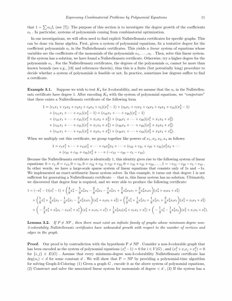
Example 3.1. Suppose we wish to test K4 for 3-colorability, and we assume that the αi in the Nullstellen-satz certificate have degree 1. After encoding K4 with the system of polynomial equations, we “conjecture”that there exists a Nullstellensatz certificate of the following form
1 = (c1x1 + c2x2 + c3x3 + c4x4 + c5)(x31 − 1) + (c6x1 + c7x2 + c8x3 + c9x4 + c10)(x3
2 − 1)
+ (c11x1 + · · ·+ c15)(x33 − 1) + (c16x1 + · · ·+ c20)(x3
4 − 1)
+ (c21x1 + · · ·+ c25)(x21 + x1x2 + x2
2) + (c26x1 + · · ·+ c30)(x21 + x1x3 + x2
3)
+ (c31x1 + · · ·+ c35)(x21 + x1x4 + x2
4) + (c36x4 + · · ·+ c40)(x22 + x2x3 + x2
3)
+ (c41x1 + · · ·+ c45)(x22 + x2x4 + x2
4) + (c46x1 + · · ·+ c50)(x23 + x3x4 + x2
4).
When we multiply out this certificate, we group together like powers of x1, x2, x3, x4 as follows:
1 = c1x41 + · · ·+ c13x
43 + · · ·+ c8x
32x3 + · · ·+ (c22 + c21 + c27 + c32)x2
1x2 + · · ·+ (c35 + c45 + c50)x2
4 + · · ·+ (−c15 − c20 − c5 − c10).
Because the Nullstellensatz certificate is identically 1, this identity gives rise to the following system of linearequations: 0 = c1, 0 = c13, 0 = c8, 0 = c22 + c21 + c27 + c32, 0 = c35 + c45 + c50, . . . , 1 = −c15− c20− c5− c10 .In other words, we have a large-scale sparse system of linear equations that consists only of 1s and −1s.We implemented an exact-arithmetic linear system solver. In this example, it turns out that degree 1 is notsufficient for generating a Nullstellensatz certificate — that is, this linear system has no solution. Ultimately,we discovered that degree four is required, and we were able to produce the following certificate:
1 = (−x31 − 1)(x3
1 − 1) +
„4
9x4
4 −5
9x3
4x2 −2
9x3
4x3 −4
9x3
4x1 +2
9x2
4x2x1 +2
9x2
4x3x1
«(x2
4 + x2x4 + x22)
+
„1
9x4
4 +2
9x3
4x2 −1
9x3
4x1 −2
9x2
4x2x1
«(x2
2 + x3x2 + x23) +
„2
9x4
4 +1
9x3
4x2 +1
9x3
4x1 +2
9x2
4x2x1
«(x2
4 + x3x4 + x23)
+
„− 2
3x4
4 + x34x1 − x4x
31 + x4
1
«(x2
4 + x1x4 + x21) +
1
3x3
4x2(x22 + x1x2 + x2
1) +
„− 1
3x4
4 −1
3x3
4x2
«(x2
3 + x1x3 + x21).
Lemma 3.2. If P 6= NP , then there must exist an infinite family of graphs whose minimum-degree non-3-colorability Nullstellensatz certificates have unbounded growth with respect to the number of vertices andedges in the graph.
Proof. Our proof is by contradiction with the hypothesis P 6= NP . Consider a non-3-colorable graph thathas been encoded as the system of polynomial equations (x3
i −1) = 0 for i ∈ V (G) , and (x2i +xixj +x2
j ) = 0for i, j ∈ E(G) . Assume that every minimum-degree non-3-colorability Nullstellensatz certificate hasdeg(αi) < d for some constant d . We will show that P = NP by providing a polynomial-time algorithmfor solving Graph-3-Coloring: (1) Given a graph G , encode it as the above system of polynomial equations,(2) Construct and solve the associated linear system for monomials of degree < d , (3) If the system has a

12 J.A. De Loera, J. Lee, S. Margulies, S. Onn
solution, a Nullstellensatz certificate exists, and the graph is non-3-colorable: Return no, (4) If the systemdoes not have a solution, there does not exist a Nullstellensatz certificate, and the graph is 3-colorable:Return yes.
Now we analyze the running time of this algorithm. In Step 1, our encoding has one polynomial equationper vertex and one polynomial equation per edge. Since there are O(n2) edges in a graph, our polynomialsystem has n+n2 = O(n2) equations. Since every equation only contains coefficients ±1 and is of degree threeor less, encoding the graph as the above system of polynomial equations clearly runs in polynomial-time.
For Step 2, we note that by Corollary 3.2b of [34], if a system of linear equations Ax = b has a solution,then it has a solution polynomially-bounded by the bit-sizes of the matrix A and the vector b (see [34] for adefinition of bit-size). In this case, the vector b contains only zeros and ones. To calculate the bit-size of A ,we recall our assumption that, for every αi , deg(αi) < d for some constant d . Therefore, an upper boundon the number of terms in each αi is the total number of monomials in n variables of degree less than orequal to d . Therefore, the number of terms in each αi is(
n+ d− 1n− 1
)+(n+ d− 2n− 1
)+ · · ·+
(n− 1n− 1
)= O(nd) +O(nd−1) + · · ·+O(1) = O(nd).
Since there are O(n2) equations, there are at most O(nd+2) unknowns in the linear system, and thus,O(nd+2) columns in A . Since the vertex equations (x3
i − 1) = 0 have two terms, and the edge equations(x2i + xixj + x2
j ) = 0 have 3 terms, there are O(nd+2) terms in the expanded Nullstellensatz certificate, andO(nd+2) rows in A . Since entries in A are 0,±1 , the matrix A contains only entries of bit-size at most 2.Therefore, the bit-sizes of both A and b are polynomially-bounded in n , and by Theorem 3.3 of [34], thelinear system can be solved in polynomial-time.
Therefore, we have demonstrated a polynomial-time algorithm for solving Graph-3-Coloring, and sinceGraph-3-Coloring is NP-Complete ([12]), this implies P = NP , which contradicts our hypothesis. Therefore,deg(αi) d for any constant d .
Thus, in the linear algebra approach to finding a minimum-degree Nullstellensatz certificate, the existenceof a universal constant bounding the degree is impossible under a well-known hypothesis of complexity theory.Clearly, a similar result can be obtained for other encodings (for a generalized statement see [26]). Note thatthe linear algebra method does not rely on any property that is unique to a particular combinatorial or NP-Complete problem; the only assumption is that the problem can be represented as a system of polynomialequations. We will use it to find Nullstellensatz certificates of non-3-colorability and sizes of stable sets ofgraphs.
We remark that this linear algebra method finds not only a Nullstellensatz certificate (if it exists), butit finds one of minimum possible degree. With our implementation, we ran several experiments. We quicklyfound out that the systems of linear equations are numerically unstable, thus it is best to use exact arithmeticto solve them. The systems of linear equations are also quite large in practice, as the bound on the degreeof the polynomial coefficients grows. Thus we need ways to reduce the number of unknowns.
We will not discuss here ad hoc methods that depend on the particular polynomial system at hand (see [26]for methods specific to 3-colorability), but one rather useful general trick is to randomly eliminate variablesin the above procedure. Instead of allowing all monomials of degree ≤ d to appear in the construction of thelinear system of equations, we can randomly set unknowns in the linear system of equations to 0 — e.g., seteach variable to 0 with probability p , independently, to get a smaller system.
In Figure 4, we see the results of the probabilistic search for smaller Nullstellensatz certificates. On thex-axis is the probability p of keeping an unknown in the linear system. Thus, if p = 0.1 , 90% of the time weset the unknown to 0, and only 10% of the time, we keep it in the system. For the cliques and odd wheels, weknow that there is always a certificate of degree four. For every probability 0.1, 0.2, . . . , 1 we performed 100searches for a degree four certificate. For both the cliques and the odd wheels, at p = 0.1 and p = 0.2 , wealmost never found a certificate. But for p = 0.4 , we found certificates 95% of the time. In practice this idea
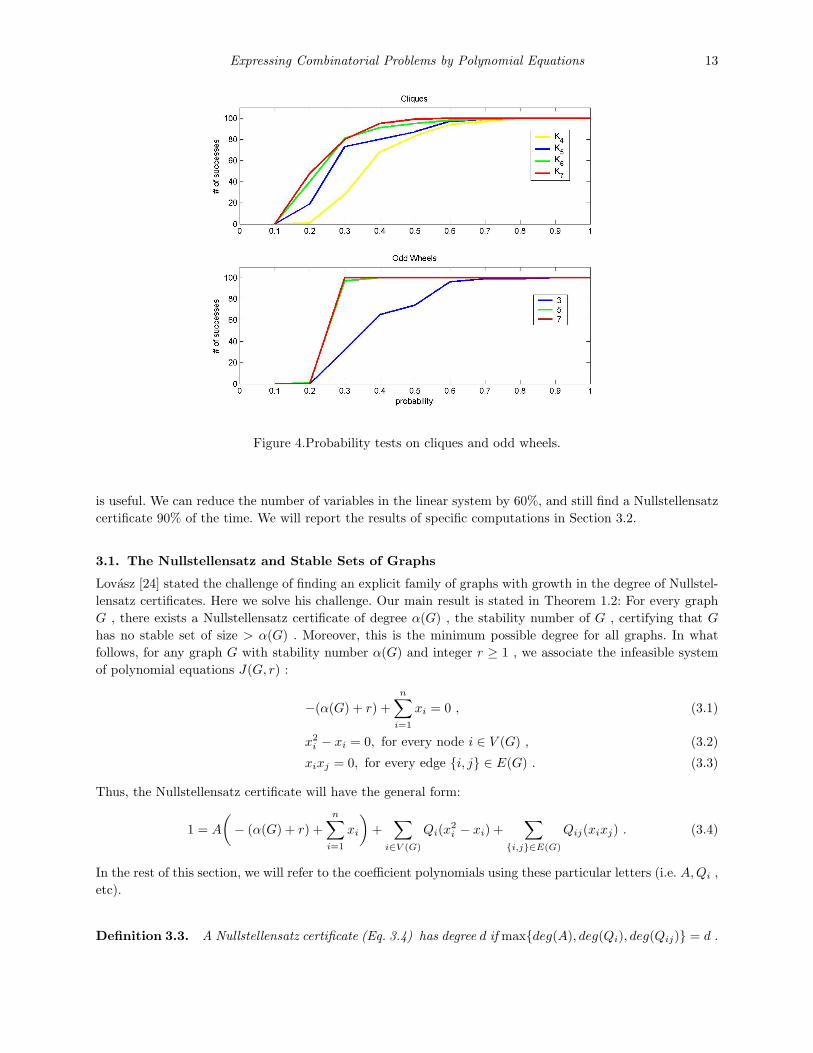
Expressing Combinatorial Problems by Polynomial Equations 13
Figure 4.Probability tests on cliques and odd wheels.
is useful. We can reduce the number of variables in the linear system by 60%, and still find a Nullstellensatzcertificate 90% of the time. We will report the results of specific computations in Section 3.2.
3.1. The Nullstellensatz and Stable Sets of Graphs
Lovasz [24] stated the challenge of finding an explicit family of graphs with growth in the degree of Nullstel-lensatz certificates. Here we solve his challenge. Our main result is stated in Theorem 1.2: For every graphG , there exists a Nullstellensatz certificate of degree α(G) , the stability number of G , certifying that Ghas no stable set of size > α(G) . Moreover, this is the minimum possible degree for all graphs. In whatfollows, for any graph G with stability number α(G) and integer r ≥ 1 , we associate the infeasible systemof polynomial equations J(G, r) :
−(α(G) + r) +n∑i=1
xi = 0 , (3.1)
x2i − xi = 0, for every node i ∈ V (G) , (3.2)
xixj = 0, for every edge i, j ∈ E(G) . (3.3)
Thus, the Nullstellensatz certificate will have the general form:
1 = A
(− (α(G) + r) +
n∑i=1
xi
)+
∑i∈V (G)
Qi(x2i − xi) +
∑i,j∈E(G)
Qij(xixj) . (3.4)
In the rest of this section, we will refer to the coefficient polynomials using these particular letters (i.e. A,Qi ,etc).
Definition 3.3. A Nullstellensatz certificate (Eq. 3.4) has degree d if maxdeg(A), deg(Qi), deg(Qij) = d .

14 J.A. De Loera, J. Lee, S. Margulies, S. Onn
Lemma 3.4. For any graph G and a Nullstellensatz certificate
1 = A
(− (α(G) + r) +
n∑i=1
xi
)︸ ︷︷ ︸
B
+∑
i∈V (G)
Qi(x2i − xi) +
∑i,j∈E(G)
Qij(xixj) (3.5)
certifying that G has no stable set of size (α(G)+r) (with r ≥ 1), we can construct a “reduced” Nullstellensatzcertificate
1 = A′(− (α(G) + r) +
n∑i=1
xi
)+
∑i∈V (G)
Q′i(x2i − xi) +
∑i,j∈E(G)
Q′ij(xixj),
such that
1. The coefficient A′ multiplying −(α(G) + r) +∑ni=1 xi has only square-free monomials supported on stable
sets of G , and thus deg(A′) ≤ α(G) .2. maxdeg(A), deg(Qi), deg(Qij) = maxdeg(A′), deg(Q′i), deg(Q′ij) . Thus, if the original Nullstellensatz
certificate has minimum-degree, the “reduced” certificate also has minimum-degree.
Proof. Let I be the ideal generated by x2i −xi (for every node i ∈ V (G)), and xixj ( for every edge i, j ∈
E(G)). We apply reductions modulo I to Eq. 3.5. If a non-square-free monomial appears in polynomial A , sayxα1i1xα2i2· · ·xαkik with at least one αj > 1 , then we can subtract the polynomial xα1
i1xα2i2· · · , xαj−2
ijxαkik B(x2
ij−
xij ) from AB and simultaneously add it to∑Qs(x2
s − xs) . Thus, eventually we obtain a new certificatethat has only square-free monomials in A′ . Furthermore, if Q′s has new monomials, they are of degree lessthan or equal to what was originally in A .
Similarly, if xi1xi2 · · ·xik appears in A , but xi1xi2 · · ·xik contains an edge i, j ∈ E(G) (if xixj dividesxi1xi2 · · ·xik), then we can again subtract B(xi1xi2 · · ·xik/xixj)(xixj) from AB , and, at the same time, addit to
∑i,j∈E(G)Qijxixj . Furthermore, the degree is maintained, and we have reached the form we claim
exists for A′ .
We now show that, for every graph, there exists an explicit Nullstellensatz certificate of degree α(G) .
Theorem 3.5. Given a graph G , there exists a Nullstellensatz certificate of degree α(G) certifying thenon-existence of stable sets of size greater than α(G) .
Proof. The proof is an algorithm to construct the explicit Nullstellensatz certificate for the non-existenceof a stable set of size α(G) + r, with r ≥ 1 . First, let us establish some notation: Let S(i, G) be the setof all stable sets of size i in G . We index nodes in the graph by integers, thus stable sets in G are subsetsof integers. When we refer to a monomial xd1xd2 · · ·xdi as a “stable set”, we mean d1, . . . , di ∈ S(i, G) .We use “hat” notation to remove a variable from a monomial, meaning xd1xd2 · · ·xdi−1 xdixdi+1 · · ·xdk =xd1xd2 · · ·xdi−1xdi+1 · · ·xdk . Finally, let
P(i, G) :=∑
d1,d2,...,di∈S(i,G)
xd1xd2 · · ·xdi , and P(0, G) := 1 .
When P(i, G) is ordered lexicographically, we denote Pj(i, G) as the j-th term. We also define the constants
CGi :=iCGi−1
α(G) + r − i, and CG0 :=
1α(G) + r
.
Our main claim is that we can construct explicit coefficients A,Qi, Qij of degree less than or equal to α(G)

Expressing Combinatorial Problems by Polynomial Equations 15
********************************************
ALGORITHM (Nullstellensatz certificate construction)
INPUT: A graph G(V,E), associated polynomials P(i, G) , α(G), r
OUTPUT: polynomials (A,Qi, Qij) such that AB + C = 1 is true
0 A← −Pα(G)i=0 CGi P(i, G)
1 Qi ← 0 , for i = 1 . . . |V |2 Qij ← 0 , for i, j ∈ E(G)
3 for i← 0 to α(G)
4 for j ← 1 to # of monomials in P(i, G)
5 for k ← 1 to |V |6 Let Pj(i, G) = xd1xd2 · · ·xdi7 if Pj(i, G)xk is a square-free stable set
8 (rule 1) Qk ← Qk + CGi+1xd1xd2 · · ·xdi9 else if Pj(i, G)xk is a square-free non-stable set
10 Choose an edge l, 1 ≤ l ≤ i, so that (k, dl) is an edge of G
12 (rule 2) Qkdl ← Qkdl + CGi xd1xd2 · · ·xdl−1 cxdlxdl+1 · · ·xdi13 end if
14 end for
15 end for
16 end for
17 return A,Qi, Qij*******************************************
Figure 5.Nullstellensatz certificate construction
such that the following identity is satisfied
1 = A
(− (α(G) + r) +
n∑i=1
xi
)︸ ︷︷ ︸
B
+∑
i,j∈E(G)
Qijxixj +n∑i=1
Qi(x2i − xi)︸ ︷︷ ︸
C
.
We do so by the algorithm of Figure 5. In Figure 5 and in what follows, AB and C refer to parts of theequation as marked above.
It is clear that the algorithm terminates for any finite graph, since the number of iterations of each forloop is finite. To prove correctness of the algorithm, we demonstrate that the following statement is true foreach iteration of the for loop beginning in line 3:
Prior to the m-th iteration, AB + C − 1 only contains terms of degree m+ 1 or greater.Furthermore, all terms of degree m+ 1 are square-free.
(∗)
When the for loop is initialized, A is set to the polynomial −∑α(G)i=0 CGi P(i, G) , and Qi, Qij are set to
zero. Therefore, prior to the 0-th iteration, C = 0 and AB + C − 1 = AB − 1 . Since the constant term inAB is equal to
−CG0 P(0, G)(− (α(G) + r)
)= − 1
α(G) + r
(− (α(G) + r)
)= 1 ,
this implies that AB−1 only contains terms of degree 1 or higher. Furthermore, linear terms are by definitionsquare-free. Thus, (∗) is true at initialization.
Now we must show that if (∗) is true prior to the m-th iteration of the for loop, then it will be true priorto the (m+ 1)-th iteration. Assume then, that prior to the m-th iteration, AB +C − 1 only contains termsof degree m+ 1 or greater, and that all terms of degree m+ 1 are square-free. We must show that prior tothe (m+ 1)-th iteration, AB +C − 1 only contains terms of degree m+ 2 or greater, and furthermore, that
16 J.A. De Loera, J. Lee, S. Margulies, S. Onn
all terms of degree m + 2 are square-free. Prior to the m-th iteration, there are only two kinds of terms ofdegree m+1 in AB+C−1 : (1) terms corresponding to square-free, stable sets, and (2) terms correspondingto square-free, non-stable sets. We will show that both kinds of terms cancel during the m-th iteration.
• Let xd1xd2 · · ·xdm+1 be any square-free, stable set monomial in AB + C − 1 of degree (m + 1) . Sinced1, d2, . . . , dm+1 is a stable set, all subsets of size m are likewise stable sets and appear as summandsin P(m,G) . Consider the coefficient of xd1xd2 · · ·xdm+1 in C . During the m-th iteration, we apply rule1 and create this monomial
(m+1m
)times in C . Since this monomial is created by the multiplication of
xd1xd2 · · · xdk · · ·xdm+1 with (x2dk− xdk) , the coefficient for xd1xd2 · · ·xdm+1 in C is
−(m+ 1m
)CGm+1 = −(m+ 1)CGm+1
Now we will calculate the coefficient of this same monomial in AB . This monomial is created in twoways, (1) multiplying −CGmxd1xd2 · · ·xdj−1 xdjxdj+1 · · ·xdm+1 by xdj (repeated (m+1) times, once for eachxdj ), or (2) multiplying −CGm+1xd1xd2 · · ·xdm+1 by −(α(G) + r) (occurring exactly once). Therefore, thecoefficient of xd1xd2 · · ·xdm+1 in AB is
− CGm+1
(− (α(G) + r)
)− (m+ 1)CGm
= α(G)CGm+1 + rCGm+1 −(m+ 1)CGm
α(G) + r − (m+ 1)(α(G) + r − (m+ 1))
= α(G)CGm+1 + rCGm+1 − CGm+1
(α(G) + r − (m+ 1)
)= α(G)CGm+1 + rCGm+1 − α(G)CGm+1 − rCGm+1 + (m+ 1)CGm+1
= (m+ 1)CGm+1 .
Therefore, the coefficient for any square-free stable-set monomial in AB + C − 1 is
(m+ 1)CGm+1︸ ︷︷ ︸from AB
−(m+ 1)CGm+1︸ ︷︷ ︸from C
= 0 .
• Now, consider any square-free non-stable-set monomial xd1xd2 · · ·xdm+1 in AB + C − 1 of degree m+ 1 .Consider all
(m+1m
)subsets of d1, d2, . . . , dm+1 , and let M be the number of stable sets among those(
m+1m
)subsets. Each of those M subsets appears as a summand in P(m,G) . Therefore, the monomial
xd1xd2 · · ·xdm+1 is created M times in AB , and M times in C , by M applications of rule 2 . Therefore,the coefficient for any square-free non-stable set monomial xd1xd2 · · ·xdm+1 in AB + C − 1 is
−MCGm︸ ︷︷ ︸from AB
+MCGm︸ ︷︷ ︸from C
= 0 .
Finally, consider any non-square-free monomial xd1xd2 · · ·x2dl· · ·xdm+1 in AB + C − 1 of degree m + 2 .
We note that d1, d2, . . . , dm+1 is an stable set. To see this, note that every non-square-free monomialin AB is created by the product of an stable set with a linear term, and every non-square-free monomialin C is created by the product of an stable set with (x2
dl− xdl) for some dl . During the m-th iteration,
during applications of rule 1, xd1xd2 · · · xdl · · ·xdm+1 is added to Qdl . Therefore, when Qdl is subsequentlymultiplied by (x2
dl− xdl) , the monomial xd1xd2 · · ·x2
dl· · ·xdm+1 is created. To summarize, this monomial is
created in only one way in AB and only one way in C . Therefore, the coefficient for xd1xd2 · · ·x2dl· · ·xdm+1
in AB + C − 1 is
−CGm+1︸ ︷︷ ︸from AB
+CGm+1︸ ︷︷ ︸from C
= 0 .
Therefore, we have proven that (∗) is valid prior to every iteration of the for loop. Finally, upon termina-tion, i = α(G) + 1 . Therefore, by (∗), we know that AB+C−1 only contains monomials of degree α(G) + 2or greater. However, there are no terms of degree α(G) + 2 in AB since deg(AB) = α(G) + 1 . Additionally,during the α(G)-th iteration, P(α(G), G)xk is never an stable set. Therefore, only applications of rule 2

Expressing Combinatorial Problems by Polynomial Equations 17
occur during the last iteration, and the final degrees of Qi, Qij are less than or equal to α(G)−1 . Therefore,the monomial in C of greatest degree is of degree α(G) + 1 . Thus, there are no monomials in AB + C − 1of degree α(G) + 2 or greater, and upon termination, AB + C − 1 = 0 .
We have then shown that we can construct A,Qi, Qij such that
1 =(−α(G)∑i=0
C(i, G)P(i, G))
︸ ︷︷ ︸A
(− (α(G) + r) +
n∑i=1
xi
)︸ ︷︷ ︸
B
+∑
i,j∈E(G)
Qijxixj +n∑i=1
Qi(x2i − xi)︸ ︷︷ ︸
C
.
Since deg(Qi),deg(Qij) ≤ (α(G)− 1) , and deg(A) = α(G) , this concludes our proof.
Example 3.6. We display a certificate found by our algorithm. In Figure 6 is the Turan graph T (5, 3) .It is clear that α(T (5, 3)) = 2 . Therefore, we “test” for a stable set of size 3.
Figure 6.Turan graph T (5, 3)
The certificate constructed by our algorithm is
1 =(− 1
3(x1x2 + x3x4
)− 1
6(x1 + x2 + x3 + x4 + x5
)− 1
3
)(x1 + x2 + x3 + x4 + x5 − 3)+(
13x4 +
13x2 +
13
)x1x3 +
(13x2 +
13
)x1x4 +
(13x2 +
13
)x1x5 +
(13x4 +
13
)x2x3+(
13
)x2x4 +
(13
)x2x5 +
(13x4 +
13
)x3x5 +
(13
)x4x5 +
(13x2 +
16
)(x2
1 − x1)+(13x1 +
16
)(x2
2 − x2) +(
13x4 +
16
)(x2
3 − x3) +(
13x3 +
16
)(x2
4 − x4) +(
16
)(x2
5 − x5) .
Note that the coefficient for the stable set polynomial contains every stable set, and further note thatevery monomial in every coefficient is also indeed a stable set.
We will now prove that the stability number α(G) is the minimum-degree for any Nullstellensatz certificatefor the non-existence of a stable set of size greater than α(G) . To prove this, we rely on two propositions.
Proposition 3.7. Given a graph G , let M = d1, d2, . . . , d|M | be any maximal stable set in G . Let
1 = A
(− (α(G) + r) +
n∑i=1
xi
)+
∑i,j∈E(G)
Qijxixj +n∑i=1
Qi(x2i − xi)
be a Nullstellensatz certificate for the non-existence of a stable set of size α(G) + r (with r ≥ 1), and let
1 = A′(− (α(G) + r) +
n∑i=1
xi
)︸ ︷︷ ︸
B
+∑
i,j∈E(G)
Q′ijxixj︸ ︷︷ ︸C
+n∑i=1
Q′i(x2i − xi)︸ ︷︷ ︸
D
(3.6)
be the reduced certificate via Lemma 3.4. Then, for i ∈ 1, . . . , |M | , the linear term xdi appears in A′ witha non-zero coefficient.

18 J.A. De Loera, J. Lee, S. Margulies, S. Onn
Proof. Our proof is by contradiction. Assume that xdi does not appear in A′ with a non-zero coefficient.By inspection of Eq. 3.6, we see that A′ must contain the constant term a0 = −(α(G) + r) . Therefore, theterm a0xdi appears in A′B . However, a0xdi does not cancel within A′B since xdi does not appear in A′ byassumption. Therefore, a0xdi must cancel with a term elsewhere in the certificate. Specifically, since C onlycontains terms multiplying edge monomials, a0xdi must cancel with a term in D . But the linear term a0xdiis generated in D in only one way: a0 must multiply (x2
di− xdi) Therefore,
Q′di = other terms + a0 .
But when a0 multiplies (x2di− xdi) , this not only generates −a0xdi , which neatly cancels its counterpart in
A′B , but it also generates the cross-term a0x2di
, which must cancel elsewhere in the certificate. However,x2di
does not cancel with a term C , since C contains only terms multiplying edge monomials, and x2di
doesnot cancel with a term in A′B , since A′ contains only terms corresponding to square-free stable sets andalso because A′ does not contain xdi by assumption. Therefore, a0x
2di
must cancel elsewhere in D . There isonly one way to generate a second x2
diterm in D: a0xdi must multiply (x2
di− xdi) . Therefore,
Q′di = other terms + a0xdi + a0 .
Now, we assume
Q′di = other terms + a0xkdi + a0x
k−1di· · ·+ a0x
2di + a0xdi + a0 .
When a0xkdi
multiplies (x2di− xdi) , this generates a cross term of the form a0x
k+2di
. This term must cancelelsewhere in the certificate. As before, a0x
k+2di
does not cancel with a term in C , since C contains only termsmultiplying edge monomials, and a0x
k+2di
does not cancel with a term in A′B , since A′ contains only termscorresponding to square-free stable sets. Therefore, a0x
k+2di
must cancel elsewhere in D . But as before, thereis only one way to generate a second a0x
k+2di
term in D: a0xk+1di
must multiply (x2di− xdi) . Therefore,
Q′di = other terms + a0xk+1di
+ a0xkdi + · · ·+ a0x
2di + a0xdi + a0.
To summarize, we have inductively shown that in order to cancel lower-order terms, we are forced to generateterms of higher and higher degree. In other words, Qdi contains an infinite chain of monomials increasingin degree. Since deg(Q′di) is finite, this is clearly a contradiction.
Therefore, xdi must appear in A′ with a non-zero coefficient.
Proposition 3.8. Given a graph G , let M = d1, d2, . . . , d|M | be any maximal stable set in G , and letc1, c2, . . . , ck+1 be any (k + 1)-subset of M with k < |M | . Let
1 = A
(− (α(G) + r) +
n∑i=1
xi
)+
∑i,j∈E(G)
Qijxixj +n∑i=1
Qi(x2i − xi)
be a Nullstellensatz certificate for the non-existence of a stable set of size α(G) + r (with r ≥ 1), and let
1 = A′(− (α(G) + r) +
n∑i=1
xi
)︸ ︷︷ ︸
B
+∑
i,j∈E(G)
Q′ijxixj︸ ︷︷ ︸C
+n∑i=1
Q′i(x2i − xi)︸ ︷︷ ︸
D
be the reduced certificate via Lemma 3.4. If xc1xc2 · · ·xck appears in A′ with a non-zero coefficient, thenxc1xc2 · · ·xckxck+1 also appears in A′ with a non-zero coefficient.
Proof. Our proof is by contradiction. Assume xc1xc2 · · ·xck with k < |M | appears in A′ with a non-zerocoefficient, but xc1xc2 · · ·xckxck+1 does not. Since xc1xc2 · · ·xck appears in A′ , xc1xc2 · · ·xckxck+1 clearlyappears in A′B and must cancel elsewhere in the certificate. However, xc1xc2 · · ·xckxck+1 does not cancelwith a term in C , since C contains only terms multiplying edge monomials and c1, c2, . . . , ck+1 is a

Expressing Combinatorial Problems by Polynomial Equations 19
stable set. Furthermore, xc1xc2 · · ·xckxck+1 does not cancel with a term in A′B , since A′ does not containxc1xc2 · · ·xckxck+1 by assumption. Therefore, xc1xc2 · · ·xckxck+1 must cancel with a term in D , and for atleast one i , xc1xc2 · · · xci · · ·xckxck+1 appears in Qci with a non-zero coefficient.
When xc1 · · · xci · · ·xckxck+1 multiplies (x2ci−xci) , this generates a cross term of the form xc1 · · ·x2
ci · · ·xckxck+1
which must cancel elsewhere in the certificate. Letm1 = xc1xc2 · · ·xckxck+1 andm2 = xc1xc2 · · ·x2ci · · ·xckxck+1 .
Note that deg(m2) = deg(m1) + 1 . As before, m2 does not cancel with a term in C , since C contains onlyterms multiplying edge monomials, and m2 does not cancel with a term in A′B , since A′ contains onlyterms corresponding to square-free stable sets. Therefore, m2 must cancel elsewhere in D .
In order to cancel m2 in D , for some cj , we must subtract one from the cj-th exponent, and then multiplythis monomial by (x2
cj − xcj ) . However, this generates a cross-term m3 = xc1xc2 · · ·x2ci · · ·x
2cj · · ·xckxck+1
where deg(m3) = deg(m2) + 1 . Note that in the case when j = i , m3 = xc1xc2 · · ·x3ci · · ·xckxck+1 , but
deg(m3) still is equal to deg(m2) + 1 .Inductively, consider the n-th element in this chain, and assume it appears with a non-zero coefficient in
some Qcj . Let
mn = xα1c1 x
α2c2 · · ·x
αk+1ck+1
,
where αi ≥ 1 for i ∈ 1, . . . , k+ 1 . When mn multiplies (x2cj − xcj ) , this generates the cross-term mnx
2cj .
This term must cancel elsewhere in the certificate. As before, mnx2cj does not cancel with a term C , since
C contains only terms multiplying edge monomials, and mnx2cj does not cancel with a term in A′B , since
A′ contains only terms corresponding to square-free stable sets and xc1xc2 · · ·xckxck+1 does not appear inA′ by assumption. Therefore, mnx
2cj must cancel elsewhere in D .
In order to cancel mnx2cj in D , note that
mncj2 = xα1
c1 xα2c2 · · ·x
αj+2cj · · ·xαk+1
ck+1,
and for some l , let
mn+1 = xα1c1 x
α2c2 · · ·x
αj+2cj · · ·xαl−1
cl· · ·xαk+1
ck+1.
Note that deg(mn+1) = deg(mn) + 1 . Therefore, in order to cancel mnx2cj , mn+1 multiplies (x2
cl− xcl) ,
which generates a new term of higher degree: mn+1x2cl
.To summarize, we have inductively shown that in order to cancel lower-order terms, we are forced to
generate terms of higher and higher degree. In other words, m1,m2, . . . form an infinite chain of monomialsincreasing in degree. Since deg(Q′i) is finite, this is clearly a contradiction.
Therefore, xc1xc2 · · ·xckxck+1 must appear in A′ with a non-zero coefficient.
Using Propositions 3.7 and 3.8, we can now prove the main theorem of this section.
Theorem 3.9. Given a graph G , any Nullstellensatz certificate for the non-existence of a stable set of sizegreater than α(G) has degree at least α(G) .
Proof. Our proof is by contradiction. Let
1 = A
(− (α(G) + r) +
n∑i=1
xi
)+
∑i,j∈E(G)
Qijxixj +n∑i=1
Qi(x2i − xi)
be any Nullstellensatz certificate for the non-existence of a stable set of size α(G) + r, with r ≥ 1 , such thatdeg(A),deg(Qi),deg(Qij) < α(G) , and let
1 = A′(− (α(G) + r) +
n∑i=1
xi
)︸ ︷︷ ︸
B
+∑
i,j∈E(G)
Q′ijxixj︸ ︷︷ ︸C
+n∑i=1
Q′i(x2i − xi)︸ ︷︷ ︸
D
(3.7)

20 J.A. De Loera, J. Lee, S. Margulies, S. Onn
be the reduced certificate via Lemma 3.4. The proof of Lemma 3.4 implies deg(A′) ≤ deg(A) < α(G) . LetM = d1, d2, . . . , dα(G) be any maximum stable set in G . Via Proposition 3.7, we know that xd1 appears inA′ with a non-zero coefficient, which implies (via Proposition 3.8) that xd1xd2 appears in A′ with a non-zerocoefficient, which implies that xd1xd2xd3 appears in A′ and so on. In particular, xd1xd2 · · ·xdα(G) appearsin A′ . This contradicts our assumption that deg(A′) < α(G) . Therefore, there can be no Nullstellensatzcertificate with deg(A) < α(G) , and the degree of any Nullstellensatz certificate is at least α(G) .
Propositions 3.7 and 3.8 also give rise to the following corollary.
Corollary 3.10. Given a graph G , any Nullstellensatz certificate for the non-existence of a stable set ofsize greater than α(G) contains at least one monomial for every stable set in G .
Proof. Given any Nullstellensatz certificate, we can create the reduced certificate via Lemma 3.4. Theproof of the Lemma 3.4 implies that the number of terms in A is equal to the number of terms in A′ . ViaPropositions 3.7 and 3.8, A′ contains one monomial for every stable set in G . Therefore, A also containsone monomial for every stable set in G .
This brings us to the last theorem of this section.
Theorem 3.11. Given a graph G , a minimum-degree Nullstellensatz certificate for the non-existence of astable set of size greater than α(G) has degree equal to α(G) and contains at least one term for every stableset in G .
Proof. This theorem follows directly from Theorems 3.5, 3.9, and Corollary 3.10.
Finally, our results establish new lower bounds for the degree and number of terms of Nullstellensatzcertificates. In earlier work, researchers in logic and complexity showed both logarithmic and linear growthof degree of the Nullstellensatz over finite fields or for special instances, e.g. Nullstellensatz related to thepigeonhole principle (see [5], [16] and references therein). Our main complexity result below settles a questionof Lovasz [24]:
Corollary 3.12. Given any infinite family of graphs Gn, on n vertices, the degree of a minimum-degreeNullstellensatz certificate for the non-existence of a stable set of size greater than α(G) grows as Ω(n) .Moreover, there are graphs for which the degree of the Nullstellensatz certificate grows linearly in n and,at the same time, the number of terms in the coefficient polynomials of the Nullstellensatz certificate isexponential in n .
Proof. The stability number of a graph G with n nodes and m vertices grows linearly ([14]) since
α(G) ≥ 12
((2m+ n+ 1)−
√(2m+ n+ 1)2 − 4n2
).
Finally, it is enough to remark that there exist families of graphs with linear growth in the minimum degreeof their Nullstellensatz certificates, but exponential growth in their numbers of terms. The disjoint unionof n/3 triangles has exactly 3n/3 maximal stable sets. Therefore, its Nullstellensatz certificate’s minimumdegree grows as O(n/3) , but its number of terms grows as 3n/3 (see [13] and references therein).

Expressing Combinatorial Problems by Polynomial Equations 21
3.2. The Nullstellensatz and 3-colorability
In this section, we investigate the degree growth of Nullstellensatz certificates for the non-3-colorability forcertain graphs. Curiously, every non-3-colorable graph that we have investigated so far has a minimum-degreeNullstellensatz certificate of degree four. Next, we prove that four is indeed a lower bound on the degree ofsuch certificates.
Theorem 3.13. Every Nullstellensatz certificate of a non-3-colorable graph has degree at least four.
Proof. Our proof is by contradiction. Suppose there exists a Nullstellensatz certificate of degree three orless. Such a certificate has the following form
1 =n∑i=1
Pi(x3i − 1) +
∑i,j∈E
Pij(x2i + xixj + x2
j ) , (3.8)
where Pi and Pij represent general polynomials of degree less than or equal to three. To be precise,
Pi =n∑s=1
aisx3s +
n∑s=1
n∑t=1t 6=s
bistx2sxt
+n∑s=1
n∑t=s+1
n∑u=t+1
cistuxsxtxu +n∑s=1
n∑t=1
distxsxt +n∑s=1
eisxs + fi
and
Pij =n∑s=1
aijsx3s +
n∑s=1
n∑t=1t 6=s
bijstx2sxt
+n∑s=1
n∑t=s+1
n∑u=t+1
cijstuxsxtxu +n∑s=1
n∑t=1
dijstxsxt +n∑s=1
eijsxs + fij .
Since we work with undirected graphs, note that aijs = ajis , and this fact applies to all coefficients athrough f . Note also that when i, j is not an edge of the graph, Pij = 0 and thus aijs = 0 . Again, thisfact holds for all coefficients a through f .
When Pi multiplies (x3i −1) , this generates cross-terms of the form Pix
3i and −Pi . In particular, this
generates monomials of degree six or less. Notice that Pij(x2i + xixj + x2
j ) does not generate monomials ofdegree six, only monomials of degree five or less. We begin the process of deriving a contradiction from Eq.3.8 by considering all monomials of the form x3
sx3i that appear in the expanded Nullstellensatz certificate.
These monomials are formed in only two ways: Either (1) x3s(x
3i − 1) , or (2) x3
i (x3s − 1) . Therefore, the n2
equations for x3sx
3i are as follows:
0 = a11 , (coefficient for x31x
31 = x6
1) (I.1)
0 = a12 + a21 , (coefficient for x31x
32) (I.2)
......
...
0 = an−1n + an(n−1) , (coefficient for x3(n−1)x
3n) (I.n2 − 1)
0 = ann . (coefficient for x3nx
3n = x6
n) (I.n2)
Summing equations I.1 through I.n2 , we get
0 =n∑i=1
n∑s=1
ais . (3.9)
22 J.A. De Loera, J. Lee, S. Margulies, S. Onn
Let us now consider monomials of the form x2sxtx
3i (with s 6= t). These monomials are formed in only one
way: by multiplying bistx2sxt by x3
i . Therefore, since the coefficient for x2sxtx
3i must simplify to zero in
the expanded Nullstellensatz certificate, bist = 0 for all bi . When we consider monomials of the formxsxtxux
3i (with s < t < u) , we see that cistu = 0 for all ci , for the same reasons as above.
As we continue toward our contradiction, we now consider monomials of degree three in the expandedNullstellensatz certificate. In particular, we consider the coefficient for x3
s . The monomial x3s is generated in
three ways: (1) fs(x3s−1) , (2) aisx3
s(x3i−1) (from the vertex polynomials), and (3) estsxs(x2
s+xsxt+x2t )
(from the edge polynomials). The equations for x31, . . . , x
3n are as follows:
0 = f1 −n∑i=1
ai1 +∑
t∈Adj(1)
e1t1 , (coefficient for x31) (II.1)
0 = f2 −n∑i=1
ai2 +∑
t∈Adj(2)
e2t2 , (coefficient for x32) (II.2)
......
...
0 = fn −n∑i=1
ain +∑
t∈Adj(n)
entn . (coefficient for x3n) (II.n)
Summing equations II.1 through II.n , we get
0 =n∑i=1
fi −( n∑i=1
n∑s=1
ais
)+
n∑s=1
n∑t∈Adj(s)
ests . (3.10)
Since the degree three or less Nullstellensatz certificate (Eq. 3.8) is identically one, the constant terms mustsum to one. Therefore, we know
∑ni=1 fi = −1 . Furthermore, recall that ests = 0 if the undirected edge
s, t does not exist in the graph. Therefore, applying Eq. 3.9 to Eq. 3.10, we have the following equation
1 =n∑
s,t=1,s6=t
ests . (3.11)
To give a preview of our overall proof strategy, the equations to come will ultimately show that the right-handside of Eq. 3.11 also equals zero, which is a contradiction.
Now we will consider the monomial x2sxt (with s 6= t). We recall that bist = 0 for all bi (where bist
is the coefficient for x2sxt in the i-th vertex polynomial). Therefore, we do not need to consider bist in the
equation for the coefficient of monomial x2sxt . In other words, we only need to consider the edge polynomials,
which can generate this monomial in two ways: (1) estsxs · xsxt , and (2) esitxt · x2s . The N = 2
(n2
)equations for these coefficients are:
0 = e121 +∑
i∈Adj(1)
e1i2 , (coefficient for x21x2) (III.1)
0 = e131 +∑
i∈Adj(1)
e1i3 , (coefficient for x21x3) (III.2)
......
...
0 = en(n−1)n +∑
i∈Adj(n)
eni(n−1) . (coefficient for x2nxn−1) (III.N)

Expressing Combinatorial Problems by Polynomial Equations 23
When we sum equations III.1 to III.N , we obtainn∑s=1
n∑t=1,t6=s
ests +( n∑s=1
∑t∈Adj(s)
estt
)︸ ︷︷ ︸
partial sum A
+( n∑s=1
∑t∈Adj(s)
n∑u=1,u 6=s,t
estu
)︸ ︷︷ ︸
partial sum B
= 0 . (3.12)
However, recall that estu = 0 when s, t does not exist in the graph, and also that estt = etst . Thus,we can rewrite partial sum A from Eq. 3.12 as
n∑s=1
∑t∈Adj(s)
estt =n∑s=1
n∑t=1,t6=s
estt =n∑s=1
n∑t=1,t 6=s
etst .
Substituting the above into Eq. 3.12 yields
2n∑
s,t=1,s 6=t
ests +( n∑s=1
∑t∈Adj(s)
n∑u=1,u 6=s,t
estu
)︸ ︷︷ ︸
partial sum B
= 0 . (3.13)
Finally, we consider the monomial xsxtxu (with s < t < u). We have already argued that cistu = 0 for allci (where cistu is the coefficient for xsxtxu in the i-th vertex polynomial). Therefore, as before, we needonly consider the edge polynomials, which can generate this monomial in three ways: (1) estuxu ·xsxt , (2)esutxt ·xsxu , and (3) etusxs ·xtxu . As before, these coefficients must cancel in the expanded certificate,which yields the following
(n3
)equations:
0 = e123 + e132 + e231 , (coefficient for x1x2x3) (IV.1)
0 = e124 + e142 + e241 , (coefficient for x1x2x4) (IV.2)...
......
0 = e(n−2)(n−1)n + e(n−2)n(n−1) + e(n−1)n(n−2) . (coefficient for xn−2xn−1xn) (IV.M)
Summing equations IV.1 through IV.M , we obtainn−2∑s=1
n−1∑t=s+1
n∑u=t+1
(estu + esut + etus
)= 0 . (3.14)
Now we come to the critical argument of the proof. We claim that the following equation holds:( n∑s=1
∑t∈Adj(s)
n∑u=1,u 6=s,t
estu
)= 2( n−2∑s=1
n−1∑t=s+1
n∑u=t+1
(estu + esut + etus
)). (3.15)
Notice that the left-hand and right-hand sides of this equation consist only of coefficients estu with s, t, u
distinct. Consider any such coefficient estu . Notice that estu appears exactly once on the right side of theequation. Furthermore, either estu appears exactly twice on the left side of this equation (since s ∈ Adj(t)implies t ∈ Adj(s)), or estu = 0 (since the edge s, t does not exist in the graph). Therefore, Eq. 3.15 isproven. Applying this result (and Eq. 3.14) to Eq. 3.13 gives us the following:
∑1≤s,t≤ns6=t
ests = 0 . (3.16)
But Eq. 3.16 contradicts Eq. 3.11 (1 = 0), thus there can be no certificate of degree less than four.

24 J.A. De Loera, J. Lee, S. Margulies, S. Onn
It is important to note that when we try to construct certificates of degree four or greater, the equationsfor the degree-6 monomials become considerably more complicated. In this case, the edge polynomials docontribute monomials of degree six, which causes the above argument to break.
We conclude this subsection with a result that allows us to bound the degree of a minimum-degreeNullstellensatz certificate of a particular graph, if that graph can be “reduced” to another graph whoseminimum-degree Nullstellensatz certificate is known.
Lemma 3.14.
1. If H is a subgraph of G , and H has a minimum-degree non-3-colorability Nullstellensatz certificate ofdegree k , then G also has a minimum-degree non-3-colorability Nullstellensatz certificate of degree k .
2. Suppose that a non-3-colorable graph G can be transformed to a non-3-colorable graph H via a sequenceof identifications of non-adjacent nodes of G . If a minimum-degree non-3-colorability Nullstellensatzcertificate for H has degree k , then a minimum-degree non-3-colorable Nullstellensatz certificate for Ghas degree at least k .
Proof.Proof of 1: Since H is a subgraph of G , then any Nullstellensatz certificate for non-3-colorability of H isalso a Nullstellensatz certificate for non-3-colorability of G .Proof of 2: Suppose that G has a Nullstellensatz certificate for non-3-colorability of degree less than k .The certificate has the form 1 =
∑aivi +
∑bijeij where vi = x3
i − 1 , eij = x2i + xixj + x2
j , andboth ai and bij denote polynomials of degree less than k . Since the certificate is an identity, the identitymust hold for all values of the variables. In particular, it must hold for every variable substitution xi = xjwhen the nodes are non-adjacent. In this case, the variable reassignment (pictorially represented in Figure 7)yields a Nullstellensatz certificate of degree less than k for the transformed graph H . Note that the paralleledges that may arise are irrelevant to our considerations (see such examples in Figure 7). But this is in
Figure 7.Converting G (the 5-odd-wheel) to H (the 3-odd-wheel) via node identifications.
contradiction with the assumed degree of a minimum-degree certificate for H . Therefore, any certificate forG must have degree at least k .
3.2.1. Cliques, Odd Wheels, and Nullstellensatz Certificates
Theorem 3.15. For Kn with n ≥ 4 , a minimum-degree Nullstellensatz certificate for non-3-colorabilityhas degree exactly four.
Proof. It is easy to see that K4 is a subgraph of K5 , which is a subgraph of K6 , and so on. The decisionproblem of whether K4 is 3-colorable can be encoded by the system of equations
x31 − 1 = 0 , x3
2 − 1 = 0 , x21 + x1x2 + x2
2 = 0 , x21 + x1x3 + x2
3 = 0 , x21 + x1x4 + x2
4 = 0 ,x3
3 − 1 = 0 , x34 − 1 = 0 , x2
2 + x2x3 + x23 = 0 , x2
2 + x2x4 + x24 = 0 , x2
3 + x3x4 + x24 = 0 ,

Expressing Combinatorial Problems by Polynomial Equations 25
with one equation per vertex and one equation per edge. Using the linear-algebra heuristic described at thebeginning of Section 3, we find that K4 has a degree-4 Nullstellensatz certificate for non-3-colorablility:
1 = (−x31 − 1)(x3
1 − 1) +
„4
9x44 −
5
9x34x2 −
2
9x34x3 −
4
9x34x1 +
2
9x24x2x1 +
2
9x24x3x1
«(x2
4 + x2x4 + x22)
+
„1
9x44 +
2
9x34x2 −
1
9x34x1 −
2
9x24x2x1
«(x2
2 + x3x2 + x23) +
„2
9x44 +
1
9x34x2 +
1
9x34x1 +
2
9x24x2x1
«(x2
4 + x3x4 + x23)
+
„−
2
3x44 + x3
4x1 − x4x31 + x4
1
«(x2
4 + x1x4 + x21) +
1
3x34x2(x2
2 + x1x2 + x21) +
„−
1
3x44 −
1
3x34x2
«(x2
3 + x1x3 + x21).
Because K4 has a degree-4 Nullstellensatz certificate as shown above, Kn for n ≥ 4 also has a degree-4Nullstellensatz certificate via Lemma 3.14 (1).
The odd-wheels consist of an odd-cycle rim, with a center vertex connected to all other vertices. It israther easy to see that no odd-wheel is 3-colorable. It is natural to ask about the degree of a minimum-degree Nullstellensatz certificate for non-3-colorablility.
Theorem 3.16. Given any odd-wheel, the degree of a minimum-degree Nullstellensatz certificate for non-3-colorability is four.
Proof. First, we will prove that there exists a certificate of degree four for the n-th odd-wheel. We beginby displaying a degree-4 certificate for the 3-odd-wheel:
1 =(
49x4
1 −59x3
1x2 −29x3
1x3 −49x3
1x0 +29x2
1x2x0 +29x2
1x3x0
)(x2
1 + x2x1 + x22)+(
19x4
1 +29x3
1x2 −19x3
1x0 −29x2
1x2x0
)(x2
2 + x3x2 + x23) +
13x3
1x2(x22 + x0x2 + x2
0)+(29x4
1 +19x3
1x2 +19x3
1x0 +29x2
1x2x0
)(x2
1 + x3x1 + x23) +
13x4
1(x21 + x0x1 + x2
0)+(− 1
3x4
1 −13x3
1x2
)(x2
3 + x0x3 + x20) + (−x3
1 − 1)(x31 − 1). (3.17)
For now, we denote the non-3-colorability certificate for the 3-odd-wheel as follows:
1 = α12e12 + α23e23 + α20e20 + α13e13 + α10e10 + α30e30 + α1v1,
where v1 = x31 − 1 , and eij = x2
i + xixj + x2j and α1 and αij denote polynomials of degree four in
R[x0, x1, x2, x3] . In Figure 8, we can see that the topological difference between the 3-odd-wheel and the
Figure 8.Here we show the evolution of the 3-odd-wheel to the 5-odd-wheel. This can be extended from then-th odd wheel to the (n+ 2)-th odd wheel.
5-odd-wheel is that the edge (1, 3) is lost, and the vertices 4, 5 and associated edges (3, 4), (4, 5), (5, 1), (0, 4)and (0, 5) are gained. We can exhibit an algebraic relation (or syzygy) as follows:
α13e13 = α13e15 + β34e34 + β45e45 + β01e01 + β03e03 + β04e04

26 J.A. De Loera, J. Lee, S. Margulies, S. Onn
+ β05e05 , (3.18)
where βij ∈ R[x0, x1, x2, x3, x4, x5] and deg(βij) ≤ 4 . Note that the coefficients for e13 and e15 arethe same. Recall that
α13 =29x4
1 +19x3
1x2 +19x3
1x0 +29x2
1x2x0 .
Since α13 does not contain the variable x3 , α13 ∈ R[x0, x1, x2] and not in R[x0, x1, x2, x3] . Therefore,because there exists a degree-4 certificate for the 3-odd-wheel, we can simply use the above syzygy (Eq.3.18) to substitute for the α13e13 term in the degree-4 3-odd-wheel certificate (Eq. 3.17). The resultingpolynomial is a degree-4 certificate for the 5-odd-wheel where the coefficient for e15 in the 5-odd-wheelcertificate is exactly the same as the coefficient for e13 in the 3-odd-wheel certificate (both coefficients areα13). Thus, we can again use the syzygy of Eq. 3.18 (with the variable substitutions of x4 → x6 , x5 → x7 ,and x3 → x5), and substitute for the α13e15 term in the 5-odd-wheel certificate to obtain a degree-47-odd-wheel certificate. Thus, by induction, we obtain degree-4 certificates for all odd-wheels. It remains forus to show that such a syzygy exists.
The special syzygy was found via the linear algebra heuristic described at the beginning of Section 3 and islisted below. Note that the coefficients for e13 and e15 are indeed identical and are equal to the coefficientfor e13 in the 3-odd-wheel certificate we presented earlier (Eq. 3.17).
0 = −„
2
9x41 +
1
9x31x2 +
1
9x31x0 +
2
9x21x2x0
«| z
α13
(x21 + x3x1 + x2
3)| z e13
+
„2
9x41 +
1
9x31x2 +
1
9x31x0 +
2
9x21x2x0
«| z
α13
(x21 + x5x1 + x2
5)| z e15
+
„2
9x31x0 +
1
9x1x2x0x5 −
1
9x1x2x4x5 −
1
9x1x3x2
0 −2
9x1x3x0x4 −
2
9x2x3
0 −1
9x2x2
0x4 +1
9x44
«(x2
3 + x3x4 + x24)| z
e34
+
„−
2
9x41 −
2
9x21x2x0 −
1
9x21x2x4 +
1
9x21x0x4 −
1
9x1x2x3x0 +
1
9x1x2x3x4 −
1
9x1x2x2
0 +1
9x1x2x2
4 −2
9x40
+1
9x30x4 −
1
9x44 +
1
9x34x5 −
1
9x4x3
5
«(x2
4 + x4x5 + x25)| z
e45
+
„−
1
3x1x3x2
0 −2
9x3x0x2
4 −5
9x1x2
3x0 −1
3x21x3x0 +
2
9x21x4x5 +
2
9x20x4x5 −
1
9x1x4x2
5 +2
9x23x0x4 +
2
9x2x3x2
4
+1
9x21x2x3 −
1
9x21x2x5 +
2
9x31x3 −
2
9x31x5 +
1
9x21x0x5 −
2
9x21x2
0 +2
9x21x2
4 −4
9x1x2
3x4 −2
3x1x3x0x4 −
4
9x1x0x4x5
−5
9x1x2
0x4 −4
9x1x0x2
4 −1
9x1x0x2
5 −1
9x1x2
4x5 −2
9x1x3
0 +2
9x2x2
3x0 +1
9x2x2
3x4 −1
9x2x3x2
5 +2
9x2x0x2
4 +1
3x2x3x0x4
−1
9x2x3x0x5 +
1
9x2x3
4 −4
9x33x0 −
1
3x43 −
1
9x33x4 +
2
9x23x2
4 +2
9x20x2
5 −1
9x0x3
4
«(x2
0 + x0x1 + x21)| z
e01
+
„2
9x41 +
1
9x31x2 +
4
9x31x0 +
4
9x31x4 −
1
9x21x2x4 +
1
3x21x2
3 +1
9x21x3x0 +
1
9x21x3x4 +
5
9x21x2
0 +5
9x21x0x4 +
2
9x21x2
4
−2
9x1x2x2
0 −1
9x1x2x0x4 −
1
9x1x2x0x5 +
1
9x1x2x4x5 +
1
3x1x2
3x0 +2
9x1x3x2
0 +1
3x1x3x0x4 +
1
3x23x2
0
−1
9x3x3
0 −1
9x3x2
0x4 −2
9x3x0x2
4 −2
9x40 −
2
9x30x4
«(x2
0 + x0x3 + x23)| z
e03
+
„1
9x31x5 −
2
9x21x2x3 +
1
9x21x2x5 −
4
9x21x2
3 −1
9x1x2x3x4 +
1
9x1x2x2
0 −1
9x1x2x2
4 +1
9x1x3x2
0 +2
9x1x3x0x4
+1
3x1x3
0 +1
9x1x2
0x4 +1
9x1x2
0x5 +1
9x2x3x0x5 +
1
9x2x3x2
5 +2
9x33x0 +
1
9x23x0x4 −
1
9x23x2
4 +1
3x3x3
0
+1
9x3x0x2
4 −1
9x3x3
4 +2
9x40
«(x2
0 + x0x4 + x24)| z
e04
+
„−
1
9x31x2 +
1
9x31x4 +
1
9x21x2x3 +
1
9x21x2x4 −
1
9x21x2
0 +2
9x1x2x3x0 −
1
9x1x2x3x4 +
1
9x1x2x2
0 −1
9x1x2x2
4
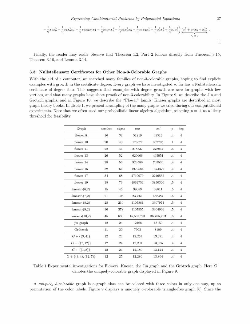
Expressing Combinatorial Problems by Polynomial Equations 27
−1
9x1x3
0 +1
9x1x2
0x4 −1
9x2x3x0x4 −
1
9x2x3x2
4 −1
9x0x2
4x5 −1
9x0x4x2
5 +1
9x24x2
5 +1
9x4x3
5
«(x2
0 + x0x5 + x25)| z
e05
.
Finally, the reader may easily observe that Theorem 1.2, Part 2 follows directly from Theorem 3.15,Theorem 3.16, and Lemma 3.14.
3.3. Nullstellensatz Certificates for Other Non-3-Colorable Graphs
With the aid of a computer, we searched many families of non-3-colorable graphs, hoping to find explicitexamples with growth in the certificate degree. Every graph we have investigated so far has a Nullstellensatzcertificate of degree four. This suggests that examples with degree growth are rare for graphs with fewvertices, and that many graphs have short proofs of non-3-colorability. In Figure 9, we describe the Jin andGrotzch graphs, and in Figure 10, we describe the “Flower” family. Kneser graphs are described in mostgraph theory books. In Table 1, we present a sampling of the many graphs we tried during our computationalexperiments. Note that we often used our probabilistic linear algebra algorithm, selecting p = .4 as a likelythreshold for feasibility.
Graph vertices edges row col p deg
flower 8 16 32 51819 49516 .4 4
flower 10 20 40 178571 362705 1 4
flower 11 22 44 278737 278844 .5 4
flower 13 26 52 629666 495051 .4 4
flower 14 28 56 923580 705536 .4 4
flower 16 32 64 1979584 1674379 .4 4
flower 17 34 68 2719979 2246535 .4 4
flower 19 38 76 4862753 3850300 .5 4
kneser-(6,2) 15 45 39059 68811 .5 4
kneser-(7,2) 21 105 230861 558484 .5 4
kneser-(8,2) 28 210 1107881 3307971 .5 4
kneser-(9,2) 36 378 1107955 3304966 .5 4
kneser-(10,2) 45 630 15,567,791 36,785,283 .5 4
jin graph 12 24 12168 13150 .4 4
Grotzsch 11 20 7903 8109 .4 4
G + (3, 4) 12 24 12,257 13,091 .4 4
G + (7, 12) 12 24 12,201 13,085 .4 4
G + (1, 8) 12 24 12,180 13,124 .4 4
G + (3, 4), (12, 7) 12 25 12,286 13,804 .4 4
Table 1.Experimental investigations for Flowers, Kneser, the Jin graph and the Grotzch graph. Here Gdenotes the uniquely-colorable graph displayed in Figure 9.
A uniquely 3-colorable graph is a graph that can be colored with three colors in only one way, up topermutation of the color labels. Figure 9 displays a uniquely 3-colorable triangle-free graph [6]. Since the

28 J.A. De Loera, J. Lee, S. Margulies, S. Onn
Figure 9.These graphs (from left to right) are (1) a uniquely 3-colorable graph, labeled with its unique3-coloring [6], (2) the Grotzsch graph, and (3) the Jin graph.
graph is uniquely 3-colorable, the addition of a single edge between two similarly-colored vertices will resultin a new non-3-colorable graph. Table 1 also details these experiments. Finally, we investigated all non-3-colorable graphs on six vertices or less: every one has a Nullstellensatz certificate of degree four.
Figure 10.3, 4 and 5 flowers (left to right). Note that the 3-flower is 3-colorable, whereas the 4 and 5 flowersare non-3-colorable. It is easy to see that only flowers that are multiples of 3 are 3-colorable.
References
[1] N. Alon, Combinatorial Nullstellensatz, Combin. Prob. and Comput., 8, (1999), 7–29.[2] N. Alon and M. Tarsi, Colorings and orientations of graphs, Combinatorica, 12, (1992), 125–134.[3] E. Babson, S. Onn and R.R. Thomas, The Hilbert zonotope and a polynomial time algorithm for universal
Grobner bases, Advances in Applied Mathematics, 30, (2003), 529–544.[4] D.A. Bayer, “The Division Algorithm and the Hilbert Scheme,” Ph.D. Thesis, Harvard University, (1982).[5] S. Buss and T. Pitassi, Good degree bounds on nullstellensatz refutations of the induction principle, IEEE
Conference on Computational Complexity, (1996), 233–242.[6] C.-Y. Chao and Z. Chen, On uniquely 3-colorable graphs, Discrete Mathematics, 112, (1993), 374–383.[7] D. Cox, J. Little and D. O’Shea, “Ideals,Varieties and Algorithms,” Springer Undergraduate Texts in Mathe-
matics, Springer-Verlag, New York, (1992).[8] D. Cox, J. Little and D. O’Shea, “Using Algebraic Geometry,” Springer Verlag Graduate Texts in Mathematics,
vol. 185, (1998).[9] J.A. De Loera, Grobner bases and graph colorings, Beitrage zur Algebra und Geometrie, 36(1), (1995), 89–96.[10] S. Eliahou, An algebraic criterion for a graph to be four-colourable, Aportaciones Matematicas, Soc. Matematica
Mexicana, Notas de Investigacion, 6, (1992), 3–27.[11] K.G. Fischer, Symmetric polynomials and Hall’s theorem, Discrete Math, 69(3), (1988), 225–234.[12] M. Garey and D. Johnson, “Computers and Intractability: A Guide to the Theory of NP-Completeness,” W.H.
Freeman and Company, Copyright 1979 Bell Telephone Laboratories, Incorporated.[13] J. Griggs, C. Grinstead and D. Guichard, The number of maximal independent sets in a connected graph ,
Discrete Mathematics, 68(2-3), (1988), 211–220.[14] J. Harant and I. Schiermeyer, On the independence number of a graph in terms of order and size, Discrete
Mathematics, 232(1-3), (2001), 131–138.[15] C.J. Hillar and T. Windfeldt, “An algebraic characterization of uniquely vertex colorable graphs,” manuscript
2006, see http://www.math.tamu.edu/~chillar/files/uniquegraphcolorings.pdf

Expressing Combinatorial Problems by Polynomial Equations 29
[16] P. Impagliazzo, P. Pudlak and J. Sgall, Lower bounds for polynomial calculus and the Groebner basis algorithm,Computational Complexity, 8, (1999), 127–144.
[17] G. Jin, Triangle-free four-chromatic graphs, Discrete Mathematics, 145, (1995), 151–170.[18] J. Kollar, Sharp effective Nullstellensatz, J. of the AMS, 1(4), (1988), 963–975.[19] M. Kreuzer and L. Robbiano, “Computational Commutative Algebra I,” Springer Verlag, Heidelberg, (2000).[20] J.B. Lasserre, Polynomials nonnegative on a grid and discrete optimization, Transactions of the AMS, 354(2),
(2001), 631–649.[21] M. Laurent, Semidefinite representations for finite varieties, Mathematical Programming, 109, (2007), 1–26.[22] M. Laurent and F. Rendl, Semidefinite programming and integer programming. In: “Handbook on Discrete
Optimization,” K. Aardal, G. Nemhauser, R. Weismantel (eds.), Elsevier B.V., (2005), 393–514.[23] S.R. Li and W.W. Li, Independence number of graphs and generators of ideals, Combinatorica, 1, (1981), 55–61.[24] L. Lovasz, Stable sets and polynomials, Discrete Mathematics, 124, (1994), 137–153.[25] L. Lovasz, Oberwolfach meeting on Geometric Convex Combinatorics, Mathematisches Forschungsinstitut Ober-
wolfach, Germany, June 2002.[26] S. Margulies, “Combinatorics, Computer Algebra and Complexity: Grobner Bases and NP-Complete Problems,”
UC Davis Ph.D. dissertation, in preparation, (2008).[27] Y. Matiyasevich, A criteria for colorability of vertices stated in terms of edge orientations, (in Russian), Discrete
Analysis (Novosibirsk), 26, (1974), 65–71.[28] Y. Matiyasevich, Some algebraic methods for calculation of the number of colorings of a graph, (in Russian),
Zapiski Nauchnykh Seminarov POMI, 293, (2001), 193–205 (available via www.pdmi.ras.ru).[29] M. Mnuk, Representing graph properties by polynomial ideals, In V. G. Ganzha, E. W. Mayr, and E. V.
Vorozhtsov, editors, “Computer Algebra in Scientific Computing, CASC 2001.” Proceedings of the Fourth Inter-national Workshop on Computer Algebra in Scientific Computing, Konstanz, Springer-Verlag, (2001), 431–444.
[30] S. Onn, Nowhere-zero flow polynomials, Journal of Combinatorial Theory, Series A, 108, (2004), 205–215.[31] P. Parrilo, Semidefinite programming relaxations for semialgebraic problems,” Mathematical Programming Ser.
B, 96(2), (2003), 293–320.[32] P. Parrilo, “An explicit construction of distinguished representations of polynomials nonnegative over finite sets,”
IfA Technical Report AUT02-02, (2002).[33] W. Schnyder, Planar graphs and poset dimension, Order, 5, (1989), 323–343.[34] A. Schrijver, “Theory of Linear and Integer Programming,” Wiley-Interscience Series in Discrete Mathematics
and Optimization, John Wiley & Sons, Chichester, West Sussex, England, 1986.[35] S.E. Shauger, Results on the Erdos-Gyarfas conjecture in K1,m-free graphs, “Proceedings of the Twenty-ninth
Southeastern International Conference on Combinatorics Graph Theory and Computing (Boca Raton, FL,1998).” Congr. Numer., 134, (1998), 61–65.
[36] A. Simis, W. Vasconcelos and R. Villarreal, On the ideal theory of graphs, J. Algebra, 167(2), (1994), 389–416.[37] M. Yannakakis, Expressing combinatorial optimization problems by linear programs, J. Comput. Syst. Sci., 43(3),
(1991), 441–466.