Exponentiation - koclab.cs.ucsb.edu

Chapter �Exponentiation

Christophe Doche

Contents in Brief

9.1 Generic methods 146Binary methods • Left-to-right 2k-ary algorithm • Sliding window method •Signed-digit recoding • Multi-exponentiation

9.2 Fixed exponent 157Introduction to addition chains • Short addition chains search • Exponentiationusing addition chains

9.3 Fixed base point 164Yao’s method • Euclidean method • Fixed-base comb method

Given an element x of a group (G,×) and an integer n ∈ Z one describes in this chapter efficientmethods to perform the exponentiation xn. Only positive exponents are considered since xn =(1/x)−n but nothing more is assumed especially regarding the structure and the properties of G.See Chapter 11 for specific improvements concerning finite fields. Two elementary operations areused, namely multiplications and squarings. The distinction is made for performance reasons sincesquarings can often be implemented more efficiently; see Chapters 10 and 11 for details. In thecontext of elliptic and hyperelliptic curves, the computations are done in an abelian group denotedadditively (G,⊕). The equivalent of the exponentiation xn is the scalar multiplication [n]P . Allthe techniques described in this chapter can be adapted in a trivial way, replacing multiplication byaddition and squaring by doubling. See Chapter 13 for additional details concerning elliptic curvesand Chapter 14 for hyperelliptic curves.

Exponentiation is a very important operation in algorithmic number theory. For example, it isintensively used in many primality testing and factoring algorithms. Therefore efficient methodshave been studied over centuries. In cryptosystems based on the discrete logarithm problem (cf.Chapter 1) exponentiation is often the most time-consuming part, and thus determines the efficiencyof cryptographic protocols like key exchange, authentication, and signature.

Three typical situations occur. The base point x and the exponent n may both vary from onecomputation to another. Generic methods will be used to get xn in this case. If the same exponentis used several times a closer study of n, especially the search of a short addition chain for n, canlead to substantial improvements. Finally, if different powers of the same element are needed, someprecomputations, whose cost can be neglected, give a noticeable speedup.

145

146 Ch. 9 Exponentiation

Most of the algorithms described in the remainder of this chapter can be found in [MEOO+ 1996,GOR 1998, KNU 1997, STA 2003, BER 2002].

9.1 Generic methods

In this section both x and n may vary. Computing xn naïvely requires n − 1 multiplications, butmuch better methods exist, some of them being very simple.

9.1.1 Binary methods

It is clear that x2k

can be obtained with only k squarings, namely x2, x4, x8, . . . , x2k

. Building uponthis observation, the following method, known for more than 2000 years, allows us to compute xn

in O(lg n) operations, whatever the value of n .

Algorithm 9.1 Square and multiply method

INPUT: An element x of G and a nonnegative integer n = (n�−1 . . . n0)2.

OUTPUT: The element xn ∈ G.

1. y ← 1 and i ← � − 1

2. while i � 0

3. y ← y2

4. if ni = 1 then y ← x × y

5. i ← i − 1

6. return y

This method is based on the equality

x(n�−1... ni+1ni)2 =(x(n�−1... ni+1)2

)2 × xni .

As the bits are processed from the most to the least significant one, Algorithm 9.1 is also referred toas the left-to-right binary method.

There is another method relying on

x(nini−1... n0)2 = xni2i × x(ni−1... n0)2

which operates from the right to the left.

Algorithm 9.2 Right-to-left binary exponentiation

INPUT: An element x of G and a nonnegative integer n = (n�−1 . . . n0)2.


1. y ← 1, z ← x and i ← 0

2. while i � � − 1 do

3. if ni = 1 then y ← y × z

§ 9.1 Generic methods 147

4. z ← z2

5. i ← i + 1

6. return y

Remarks 9.3

(i) Algorithm 9.1 is related to Horner’s rule, more precisely computing xn is similar toevaluating the polynomial

∑�−1i=0 niX

i at X = 2 with Horner’s rule.

(ii) Further enhancements may apply to the products y × x in Algorithm 9.1 since one ofthe operands is fixed during the whole computation. For example, if x is well chosen themultiplication can be computed more efficiently. Such an improvement is impossiblewith Algorithm 9.2 where different terms of approximately the same size are involvedin the products y × z.

(iii) In Algorithm 9.2, whatever the value of n, the extra variable z contains the successivesquares x2, x4, . . . which can be evaluated in parallel to the multiplication.

The next example provides a comparison of Algorithms 9.1 and 9.2.

Example 9.4 Let us compute x314. One has 314 = (100111010)2 and = 9.

Algorithm 9.1

i 8 7 6 5 4 3 2 1 0ni 1 0 0 1 1 1 0 1 0y x x2 x4 x9 x19 x39 x78 x157 x314

Algorithm 9.2

i 0 1 2 3 4 5 6 7 8ni 0 1 0 1 1 1 0 0 1z x x2 x4 x8 x16 x32 x64 x128 x256

y 1 x2 x2 x10 x26 x58 x58 x58 x314

The number of squarings is the same for both algorithms and equal to the bit length ∼ lg n of n.In fact this will be the case for all the methods discussed throughout the chapter.

The number of required multiplications directly depends on ν(n) the Hamming weight of n, i.e.,the number of nonzero terms in the binary expansion of n. On average 1

2 lg n multiplications areneeded.

Further improvements introduced below tend to decrease the number of multiplications, leadingto a considerable speedup. Many algorithms also require some precomputations to be done. Inthe case where several exponentiations with the same base have to be performed in a single run,these precomputations need to be done only once per session, and if the base is fixed in a givensystem, they can even be stored, so that their cost might become almost negligible. This is the caseconsidered in Algorithms 9.7, 9.10, and 9.23. Depending on the bit processed, a single squaringor a multiplication and a squaring are performed at each step in both Algorithms 9.1 and 9.2. Thisimplies that it can be possible to retrieve each bit and thus the value of the exponent from an anal-ysis of the computation. This has serious consequences when the exponent is some secret key. SeeChapters 28 and 29 for a description of side-channel attacks. An elegant technique, called Mont-gomery’s ladder, overcomes this issue. Indeed, this variant of Algorithm 9.1 performs a squaringand a multiplication at each step to compute xn.


Algorithm 9.5 Montgomery’s ladder

INPUT: An element x ∈ G and a positive integer n = (n�−1 . . . n0)2.


1. x1 ← x and x2 ← x2

2. for i = � − 2 down to 0 do

3. if ni = 0 then

4. x1 ← x21 and x2 ← x1 × x2

5. else

6. x1 ← x1 × x2 and x2 ← x22

7. return x1

Example 9.6 To illustrate the method, let us compute x314 using, this time, Algorithm 9.5. Startingfrom (x1, x2) = (x, x2), the next values of (x1, x2) are given below.

i 7 6 5 4 3 2 1 0

ni 0 0 1 1 1 0 1 0

(x1, x2) (x2, x3) (x4, x5) (x9, x10) (x19, x20) (x39, x40) (x78, x79) (x157, x158) (x314, x315)

See also Chapter 13, for a description of Montgomery’s ladder in the context of scalar multiplicationon an elliptic curve.

9.1.2 Left-to-right 2k2k2k2k2k2k2k2k-ary algorithm

The general idea of this method, introduced by Brauer [BRA 1939], is to write the exponent on alarger base b = 2k. Some precomputations are needed but several bits can be processed at a time.

In the following the function σ is defined by σ(0) = (k, 0) and σ(m) = (s, u) where m = 2suwith u odd.

Algorithm 9.7 Left-to-right 2k-ary exponentiation

INPUT: An element x of G, a parameter k � 1, a nonnegative integer n = (n�−1 . . . n0)2k andthe precomputed values x3, x5, . . . , x2k−1.


1. y ← 1 and i ← � − 1

2. (s, u) ← σ(ni) [ni = 2su]

3. while i � 0 do

4. for j = 1 to k − s do y ← y2

5. y ← y × xu

6. for j = 1 to s do y ← y2


7. i ← i − 1

8. return y

Remarks 9.8

(i) Lines 4 to 6 compute y2k

xni i.e., the exact analogue of y2xni in Algorithm 9.1. Toreduce the amount of precomputations, note that (y2k−s

xu)2s

= y2k

xni is actuallycomputed.

(ii) The number of elementary operations performed is lg n + lg n(1 + o(1)

)lg n/ lg lg n.

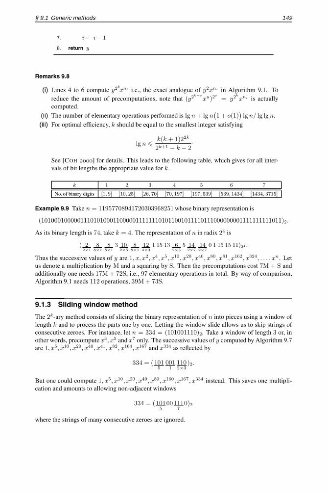
(iii) For optimal efficiency, k should be equal to the smallest integer satisfying

lg n � k(k + 1)22k

2k+1 − k − 2·

See [COH 2000] for details. This leads to the following table, which gives for all inter-vals of bit lengths the appropriate value for k.

k 1 2 3 4 5 6 7

No. of binary digits [1, 9] [10, 25] [26, 70] [70, 197] [197, 539] [539, 1434] [1434, 3715]

Example 9.9 Take n = 11957708941720303968251 whose binary representation is

(10100010000011101010001100000111111101011001011110111000000001111111111011)2.

As its binary length is 74, take k = 4. The representation of n in radix 24 is

( 22×1

88×1

88×1

3 102×5

88×1

124×3

1 15 13 62×3

5 142×7

142×7

0 1 15 15 11)24 .

Thus the successive values of y are 1, x, x2, x4, x5, x10, x20, x40, x80, x81, x162, x324, . . . , xn. Letus denote a multiplication by M and a squaring by S. Then the precomputations cost 7M + S andadditionally one needs 17M + 72S, i.e., 97 elementary operations in total. By way of comparison,Algorithm 9.1 needs 112 operations, 39M + 73S.

9.1.3 Sliding window method

The 2k-ary method consists of slicing the binary representation of n into pieces using a window oflength k and to process the parts one by one. Letting the window slide allows us to skip strings ofconsecutive zeroes. For instance, let n = 334 = (101001110)2. Take a window of length 3 or, inother words, precompute x3, x5 and x7 only. The successive values of y computed by Algorithm 9.7are 1, x5, x10, x20, x40, x41, x82, x164, x167 and x334 as reflected by

334 = (1015

0011

1102×3

)2.

But one could compute 1, x5, x10, x20, x40, x80, x160, x167, x334 instead. This saves one multipli-cation and amounts to allowing non-adjacent windows

334 = (1015

001117

0)2

where the strings of many consecutive zeroes are ignored.


Here is the general algorithm.

Algorithm 9.10 Sliding window exponentiation

INPUT: An element x of G, a nonnegative integer n = (n�−1 . . . n0)2, a parameter k � 1 andthe precomputed values x3, x5, . . . , x2k−1.


1. y ← 1 and i ← � − 1

2. while i � 0 do

3. if ni = 0 then y ← y2 and i ← i − 1

4. else

5. s ← max{i − k + 1, 0}6. while ns = 0 do s ← s + 1

7. for h = 1 to i − s + 1 do y ← y2

8. u ← (ni . . . ns)2 [ni = ns = 1 and i − s + 1 � k]

9. y ← y × xu [u is odd so that xu is precomputed]

10. i ← s − 1

11. return y

Remarks 9.11

(i) In Line 6 the index i is fixed, ni = 1 and the while loop finds the longest substring(ni . . . ns) of length less than or equal to k such that ns = 1. So u = (ni . . . ns)2 is oddand belongs to the set of precomputed values.

(ii) Only the values xu occurring in Line 9 actually need to be precomputed and not all thevalues x3, x5, . . . , x2k−1.

(iii) In certain cases it is possible to skip some squarings at the beginning, at the cost of an ad-ditional multiplication. For the sake of clarity assume that k = 5 and that the binary ex-pansion of n is (1000000)2. Then Algorithm 9.10 computes x, x2, x4, x8, x16, x32, x64.But one could perform x31 × x instead to obtain x32 directly, taking advantage of theprecomputations. However, this trick is interesting only if the first value of u is less than2k−1.

Example 9.12 With n = 11957708941720303968251 and k = 4 the sliding window methodmakes use of the following decomposition

(1015

0001100000111

70101

500011

3000001111

15111

701011

11001011

111101

13113

00000000111115

111115

110113

11)2.

The successive values of y are 1, x5, x10, x20, x40, x80, x81, x162, x324, x648, . . . , xn. In this case93 operations are needed, namely 21M + 72S, precomputations included.

9.1.4 Signed-digit recoding

When inversion in G is fast (or when x is fixed and x−1 precomputed) it can be very efficient tomultiply by either x or x−1. This can be used to save additional multiplications on the cost ofallowing negative coefficients and hence using the inverse of precomputed values. The extreme


example is the computation of x2k−1. With the binary method, cf. Algorithm 9.1, one needs k − 1squarings and k− 1 multiplications. But one could also perform k squarings to get x2k

followed bya multiplication by x−1. This remark leads to the following concept.

Definition 9.13 A signed-digit representation of an integer n in radix b is given by

n =�−1∑i=0

nibi with |ni| < b.

A signed-binary representation corresponds to the particular choice b = 2 and ni ∈ {−1, 0, 1}.It is denoted by (n�−1 . . . n0)s and usually obtained by some recoding technique. The represen-

tation is said to be in non-adjacent form, NAF for short, if nini+1 = 0, for all i � 0. It is denotedby (n�−1 . . . n0)NAF.

For example, take n = 478 and let 1̄ = −1. Then (101̄11001̄10)s is a signed-binary representationof n. The first recoding technique was proposed by Booth [BOO 1951]. It consists of replacingeach string of i consecutive 1 in the binary expansion of n by 1 followed by a string of i − 1consecutive 0 and then 1̄. For 478 = (111011110)2 it gives (1001̄10001̄0)s. Obviously, the signed-binary representation of n is not unique. However, the NAF of a given n is unique and its Hammingweight is minimal among all signed-digit representations of n. For example, the NAF of 478 is equalto (10001̄0001̄0)NAF. On average the number of nonzero terms in an NAF expansion of length is equal to /3. See [BOS 2001] for a precise analysis of the NAF density. There is a very simplealgorithm to compute it [REI 1962, MOOL 1990].

Algorithm 9.14 NAF representation

INPUT: A positive integer n = (n�n�−1 . . . n0)2 with n� = n�−1 = 0.

OUTPUT: The signed-binary representation of n in non-adjacent form (n′�−1 . . . n′

0)NAF.

1. c0 ← 0

2. for i = 0 to � − 1 do

3. ci+1 ← �(ci + ni + ni+1)/2�4. n′

i ← ci + ni − 2ci+1

5. return (n′�−1 . . . n′

0)NAF

Remarks 9.15

(i) Algorithm 9.14 subtracts n from 3n with the rule 0 − 1 = 1 and discards the leastsignificant digit of the result. For each i, ci is the carry occurring in the addition n +2n. Let si = ci + ni + ni+1 − 2ci+1 so that the binary expansion of 3n is equal to(s�−1 . . . s0n0)2. Now n′

i = ci + ni − 2ci+1 ∈ {1, 0, 1} . The following observationensures the non-adjacent property of the expansion [JOYE 2000]. If n′

i �= 0, we haveci + ni = 1, which implies that ci+1 = ni+1. So n′

i+1 = 2(ni+1 − ci+2) must be zero.

(ii) Finding a signed-binary representation in non-adjacent form can be done by table lookup.Indeed ci+1 and n′

i, computed in Lines 3 and 4, only depend on ni+1, ni and ci givingjust eight cases.

(iii) Algorithm 9.14 operates from the right to the left. Since most of the exponentiationalgorithms presented so far process the bits from the left to the right, the signed-binaryrepresentation must first be computed and stored. To enable “on the fly” recoding, which


is particularly interesting for hardware applications, cf. Chapter 26, Joye and Yen de-signed a left-to-right signed-digit recoding algorithm. The result is not necessarily innon-adjacent form but its Hamming weight is still minimal [JOYE 2000].

(iv) Algorithms 9.1, 9.2, 9.7, and 9.10 can be updated in a trivial way to deal with signed-binary representation.

(v) A generalization of the NAF is presented below; see Algorithm 9.20.

Example 9.16 Again take n = 11957708941720303968251. Algorithm 9.14 gives

n = (101000100001001̄010100101̄0000100000001̄01̄01̄0101̄00001̄001̄0000000100000000001̄01̄)NAF.

Now one can combine this representation to a sliding window algorithm of length 4 to get thefollowing decomposition

(1015

0001100001001̄

70101

500101̄

300001

10000000 1̄01̄

−50 1̄01

−30 1̄−1

0000 1̄001̄−9

0000000110000000000 1̄01̄

−5)NAF.

The number of operations, precomputations included, is 90, namely 18M + 72S.

Koyama and Tsuruoka [KOTS 1993] designed another transformation, getting rid of the conditionnini+1 = 0 but still minimizing the Hamming weight. Its average length of zero runs is 1.42 against1.29 for the NAF.

Algorithm 9.17 Koyama–Tsuruoka signed-binary recoding

INPUT: The binary representation of n = (n′�−1 . . . n′

0)2.

OUTPUT: The signed-binary representation (n� . . . n0)s of n in Koyama–Tsuruoka form.

1. m ← 0, i ← 0, j ← 0, u ← 0, v ← 0, w ← 0, y ← 0 and z ← 0

2. while i < �lg n� do

3. if n′i = 1 then y ← y + 1 else y ← y − 1

4. i ← i + 1

5. if m = 0 then

6. if y − z � 3 then

7. while j < w do nj = bj and j ← j + 1

8. nj ← −1, j ← j + 1, v ← y, u ← i and m ← 1

9. else if y < z then z ← y and w ← i

10. else

11. if v − y � 3 then

12. while j < u do nj = bj − 1 and j ← j + 1

13. nj ← 1, j ← j + 1, z ← y, w ← i and m ← 0

14. else if y > v then v ← y and u ← i

15. if m = 0 or (m = 1 and v � y) then

16. while j < i do nj = bj − m and j ← j + 1

17. nj ← 1 − m and nj+1 ← m

18. else

19. while j < u do nj = bj − 1 and j ← j + 1

20. nj ← 1 and j ← j + 1


21. while j < i do nj = bj and j ← j + 1

22. nj ← 1 and nj+1 ← 0

23. return (n� . . . n0)s

This approach gives good results when combined with the sliding window method.

Example 9.18 For the same n = 11957708941720303968251, a sliding window exponentiation oflength 4 based on the expansion given by Algorithm 9.17 corresponds to

(1015

0001100001

1000 1̄01̄1̄

−1100011

300001

10000000 1̄01̄

−500 1̄1̄01̄

−130000 1̄001̄

−900000001

10000000000 1̄01̄

−5)s.

In total 89 operations are necessary, i.e., 17M + 72S, including the precomputations.

Now one introduces a generalization of the NAF, which combines window and signed methods assuggested in [MOOL 1990] and explained in [COMI+ 1997, COH 2005].

Definition 9.19 Let w be a parameter greater than 1. Then every positive integer n has a uniquesigned-digit expansion

n =�−1∑i=0

ni2i

where

• each ni is zero or odd• |ni| < 2w−1

• among any w consecutive coefficients at most one is nonzero.

An expansion of this particular form is called width-w non-adjacent form, NAFw for short, and isdenoted by (n�−1 . . . n0)NAFw

.

In [AVA 2005a], Avanzi shows that the NAFw is optimal, in the sense that it is a recoding ofsmallest weight among all those with coefficients smaller in absolute value than 2w−1. See also[MUST 2004] for a similar result.

A generalization of Algorithm 9.14 allows us to compute the NAFw of any number n > 0.

Algorithm 9.20 NAFw representation

INPUT: A positive integer n and a parameter w > 1.

OUTPUT: The NAFw representation (n�−1 . . . n0)NAFw of n.

1. i ← 0

2. while n > 0 do

3. if n is odd then

4. ni ← n mods 2w

5. n ← n − ni

6. else ni ← 0

7. n ← n/2 and i ← i + 1

8. return (n�−1 . . . n0)NAFw


Remarks 9.21

(i) The function mods used in Line 4 of Algorithm 9.20 returns the smallest residue inabsolute value. Hence, n mods 2w belongs to [−2w−1 + 1, 2w−1].

(ii) For w = 2 the NAFw corresponds to the classical NAF, cf. Definition 9.13.

(iii) The length of the NAFw of n is at most equal to �lg n� + 1. The average density of theNAFw expansion of n is 1/(w + 1) as n tends to infinity. For a precise analysis, see[COH 2005].

(iv) A left-to-right variant to compute an NAFw expansion of an integer can be found bothin [AVA 2005a] and in [MUST 2005]. The result may differ from the expansion pro-duced by Algorithm 9.20 but they have the same digit set and the same optimal weight.

(v) Let w > 1 and precompute the values x+− 3, . . . , x+− (2w−1−1). Then in Algorithm 9.1 itis sufficient to replace the statement

4. if ni = 1 then y ← x × yby

4. if ni �= 0 then y ← xni × yto take advantage of the NAFw expansion of n = (n�−1 . . . n0)NAFw

to compute xn.

(vi) See [MÖL 2003] for a further generalization called the signed fractional window method,where only a subset of

{x+− 3, . . . , x+− (2w−1−1)

}is actually precomputed.

Example 9.22 For n = 11957708941720303968251 and w = 4 one has

n = (500010000000700050000300001000000010005000300010007000000010000000000005)NAFw

where ni = −ni. With this representation and the modification of Algorithm 9.1 explained abovexn can be obtained with 3M+S for the precomputations and then 12M+69S, that is 85 operationsin total.

9.1.5 Multi-exponentiation

The group G is assumed to be abelian in this section.It is often needed in cryptography, for example during a signature verification, cf. Chapter 1, to

evaluate xn00 xn1

1 where x0, x1 ∈ G and n0, n1 ∈ Z. Instead of computing xn00 and xn1

1 separatelyand then multiplying these terms, it is suggested in [ELG 1985] to adapt Algorithm 9.1 in thefollowing way, in order to get xn0

0 xn11 in one round. Indeed, start from y ← 1. Scan the bits of n0

and n1 simultaneously from the left to the right and do y ← y2. Then if the current bits of n0n1

are10

, 01 or 1

1 multiply by x0, x1 or x0x1 accordingly.For example, to compute x51

0 x1661 write the binary expansion of 51 and 166

51 = (00110011)2166 = (10100110)2

and apply the rules above so that the successive values of y are at each step 1, x1, x21, x0x

51, x3

0x101 ,

x60x

201 , x12

0 x411 , x25

0 x831 , and finally x51

0 x1661 .

This trick is often credited to Shamir although it is a special case of an idea of Straus [STR 1964]described below. Note that the binary coefficients of nj are denoted by nj,k. If necessary, theexpansion of nj is padded with zeroes in order to be of length .


Algorithm 9.23 Multi-exponentiation using Straus’ trick

INPUT: The elements x0, . . . , xr−1 ∈ G and the �-bit positive exponents n0, . . . , nr−1. Foreach i = (ir−1 . . . i0)2 ∈ [0, 2r − 1], the precomputed value gi =

Qr−1j=0 x

ij

j .

OUTPUT: The element xn00 · · ·xnr−1

r−1 .

1. y ← 1

2. for k = � − 1 down to 0 do

3. y ← y2

4. i ←Pr−1j=0 nj,k2j [i = (nr−1,k . . . n0,k)2]

5. y ← y × gi

6. return y

Remarks 9.24

(i) Computing xn00 . . . x

nr−1r−1 in a naïve way requires r squarings and r/2 multiplications

on average. With Algorithm 9.23, precomputations cost 2r − r− 1 multiplications, thenonly squarings and (1 − 1/2r) multiplications are necessary on average. Howeverone needs to store 2r − r values.

(ii) One can use Algorithm 9.23 to compute xn. To do so, write n = (n�−1 . . . n0)b inbase b, then set xi = xbi

and compute xn =∏�−1

i=0 xni

i . This approach can be seen as ababy-step giant-step algorithm, where the giant steps xbi

are computed first.

(iii) All the improvements of Algorithm 9.1 described previously apply to Algorithm 9.23as well. In particular the use of parallel sliding window leads to a faster method; see[AVA 2002, AVA 2005b, BER 2002] for a general overview on multi-exponentiation.

Example 9.25 Let us compute x31021. One has 31021 = (7 36 45)64, so that xn = x450 x36

1 x72

where x0 = x, x1 = x64 and x2 = x642. First precompute the gi’s

i 0 1 2 3 4 5 6 7

gi 1 x0 x1 x0x1 x2 x0x2 x1x2 x0x1x2

Then one gets

k 5 4 3 2 1 0

n2,k 0 0 0 1 1 1

n1,k 1 0 0 1 0 0

n0,k 1 0 1 1 0 1

i 3 0 1 7 4 5

y x0x1 x20x

21 x5

0x41 x11

0 x91x2 x22

0 x181 x3

2 x450 x36

1 x72

To improve Straus’ method in case of a double exponentiation within a group where inversion canbe performed efficiently, Solinas [SOL 2001] made signed-binary expansions come back into play.

Definition 9.26 The joint sparse form, JSF for short, of the -bit integers n0 and n1 is a representa-tion of the form (

n0

n1

)=(

n0,� . . . n0,0

n1,� . . . n1,0

)JSF


such that

• of any three consecutive positions, at least one is a zero column, that is for all i and allpositive j one has ni,j+k = n1−i,j+k = 0, for at least one k in {0, +− 1}

• adjacent terms do not have opposite signs, i.e., it is never the case that ni,jni,j+1 = −1• if ni,j+1ni,j �= 0 then one has n1−i,j+1 = +− 1 and n1−i,j = 0.

The joint Hamming weight is the number of positions different from a zero column.

Solinas also gives an algorithm to compute the JSF of two integers.

Algorithm 9.27 Joint sparse form recoding

INPUT: Nonnegative �-bit integers n0 and n1 not both zero.

OUTPUT: The joint sparse form of n0 and n1.

1. j ← 0, S0 = (), S1 = (), d0 ← 0 and d1 ← 0

2. while n0 + d0 > 0 or n1 + d1 > 0 do

3. �0 ← d0 + n0 and �1 ← d1 + n1

4. for i = 0 to 1 do

5. if �i ≡ 0 (mod 2) then ri ← 0

6. else

7. ri ← �i mods 4

8. if �i ≡ +− 3 (mod 8) and �1−i ≡ 2 (mod 4) then ri ← −ri

9. Si ← ri ||Si [ri prepended to Si]

10. for i = 0 to 1 do

11. if 2di = 1 + n′i then di ← 1 − di

12. ni ← �ni/2�13. j ← j + 1

14. return S0 and S1

Remarks 9.28

(i) The joint sparse form of n0 and n1 is unique. The joint Hamming weight of the JSFof n0 and n1 is equal to /2 on average and the JSF is optimal in the sense that it hasthe smallest joint Hamming weight among all joint signed representations of n0 and n1

[SOL 2001].

(ii) The naïve computation of xn00 xn1

1 involving NAF representations of n0 and n1 requires2 squarings and 2/3 multiplications on average. Only squarings and /2 multiplica-tions are necessary with the JSF, neglecting the cost of the precomputations of x0x1 andx0/x1. Applying Straus’ trick with two integers in NAF results in a Hamming weightof 5/9 on average.

(iii) In [GRHE+ 2004], Grabner et al. introduce the simple joint sparse form whose jointHamming weight is also minimal but which can be obtained in an easier way.

§ 9.2 Fixed exponent 157

Example 9.29 Let us compute x510 x166

1 . The joint NAF expansion of 51 and 166 is

51 = (0101̄0101̄)NAF

166 = (1010101̄0)NAF.

Its joint Hamming weight is 8. The JSF of 51 and 166, as given by Algorithm 9.27, is

(51166

)=(

00101̄0011101̄01̄1̄01̄0

)JSF

with a joint Hamming weight equal to 6.

The next section is devoted to the case when several exponentiations to the same exponent n haveto be performed.

9.2 Fixed exponent

The methods considered in this section essentially give better algorithms when the exponent n isfixed. They rely on the concept of addition chains. However, the computation of a short additionchain for a given exponent can be very costly. But if the exponent is to be used several times it isprobably a good investment to carry out this search.

In the following, different kinds of addition chains are discussed, then efficient methods to actu-ally find short addition chains are introduced before related exponentiation algorithms are described.

9.2.1 Introduction to addition chains

Definition 9.30 An addition chain computing an integer n is given by two sequences v and w suchthat

v = (v0, . . . , vs), v0 = 1, vs = nvi = vj + vk for all 1 � i � s with respect tow = (w1, . . . , ws), wi = (j, k) and 0 � j, k � i − 1. (9.1)

The length of the addition chain is s.A star addition chain satisfies the additional property that at each step vi = vi−1 + vk for some

k such that 0 � k � i − 1.

Note that one should write vi = vj(i) + vk(i) since the indexes depend on i. They are omitted forthe sake of simplicity. Sometimes only v is given since it is easy to retrieve w from v. For examplev = (1, 2, 3, 6, 7, 14, 15) is an addition chain for 15 of length 6. It is implicit in the computationof x15 by Algorithm 9.1. In fact binary or window methods can be seen as methods producing andusing special classes of addition chains but it is often possible to do better, that is to find a shorterchain. For instance (1, 2, 3, 6, 12, 15) computes also 15 and is of length 5.

For a given n, the smallest s for which there exists an addition chain of length s computing n isdenoted by (n). It is not hard to see that (15) = 5 but the determination of (n) can be a difficultproblem even for rather small n.As complexities of squarings and multiplications are usually slightly different, note that a carefullychosen complexity measure should take into account not only the length of the chain but also therespective numbers of squarings and multiplications involved. For example (1, 2, 4, 5, 6, 11) and


(1, 2, 3, 4, 8, 11) compute 11 and have the same length 5. However the first chain needs 3 multipli-cations whereas the latter requires only 2.

There is an abundant literature about addition chains. It is known [SCH 1975, BRA 1939] that

lg(n) + lg(ν(n)

)− 2.13 � (n) � lg(n) + lg(n)

(1 + o(1)

)/ lg(lg(n)

),

where ν(n) is the Hamming weight of n.As said before, finding an addition chain of the shortest length can be very hard. To make this pro-

cess easier, it seems harmless to restrict the search to star addition chains. But Hansen [HAN 1959]proved that for some n, the smallest being n = 12509, there is no star addition chain of minimallength (n). The shortest length (n) has been determined for all n up to 220, pruning trees to speedup the search [BLFL]. See also Thurber’s algorithm, which is able to find all the addition chains fora given n [THU 1999]. The hardness of this search depends primarily on ν(n), so that it is longer tofind the minimal length of 191 = (10111111)2 than 1048577 = (100000000000000000001)2, butthe running time can be quite long, even for small integers with a rather low density.

The concept of addition chain can be extended in at least three different ways.

Definition 9.31 An addition-subtraction chain is similar to an addition chain except that the condi-tion vi = vj + vk is replaced by vi = vj + vk or vi = vj − vk.

For example, an addition chain for 314 is v = (1, 2, 4, 8, 9, 19, 38, 39, 78, 156, 157, 314). The addi-tion–subtraction chain v = (1, 2, 4, 5, 10, 20, 40, 39, 78, 156, 157, 314) is one term shorter.

Definition 9.32 An addition sequence for the set of integers S = {n0, . . . , nr−1} is an additionchain v that contains each element of S. In other words, for all i there is j such that ni = vj .

For example, an addition sequence computing {47, 117, 343, 499, 933, 5689} is

(1, 2, 4, 8, 10, 11, 18, 36, 47 , 55, 91, 109, 117 , 226, 343 , 434, 489, 499 , 933 , 1422, 2844, 5688, 5689 ).

In [YAO 1976], it is shown that the shortest length of an addition sequence computing the set ofintegers {n0, . . . , nr−1} is less than

lg N + cr lg N/ lg lg N,

where N = maxi{ni} and c is some constant.

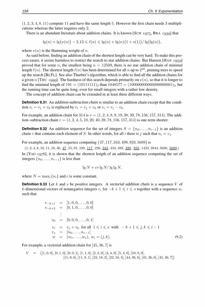
Definition 9.33 Let k and s be positive integers. A vectorial addition chain is a sequence V ofk-dimensional vectors of nonnegative integers vi for −k + 1 � i � s together with a sequence w,such that

v−k+1 = [1, 0, 0, . . . , 0, 0]v−k+2 = [0, 1, 0, . . . , 0, 0]

...v0 = [0, 0, 0, . . . , 0, 1]

vi = vj + vk for all 1 � i � s with − k + 1 � j, k � i − 1vs = [n0, . . . , nr−1]w = (w1, . . . , ws), wi = (j, k). (9.2)

For example, a vectorial addition chain for [45, 36, 7] is

V =`[1, 0, 0], [0, 1, 0], [0, 0, 1], [1, 1, 0], [2, 2, 0], [4, 4, 0], [5, 4, 0], [10, 8, 0],

[11, 9, 0], [11, 9, 1], [22, 18, 2], [22, 18, 3], [44, 36, 6], [45, 36, 6], [45, 36, 7]´


w =`(−2,−1), (1, 1), (2, 2), (−2, 3), (4, 4), (1, 5), (0, 6), (7, 7), (0, 8), (9, 9), (−2, 10), (0, 11)

´.

Since k = 3, the first three terms of V are v−2 = [1, 0, 0], v−1 = [0, 1, 0], and v0 = [0, 0, 1]. Thischain is of length 12 and is implicitly produced by Algorithm 9.23.

Addition sequences and vectorial addition chains are in some sense dual. We refer the inter-ested reader to [BER 2002, STA 2003] for details and to [KNPA 1981] for a more general ap-proach. In [OLI 1981] Olivos describes a procedure to transform an addition sequence computing{n0, . . . , nr−1} of length into a vectorial addition chain of length + r − 1 for [n0, . . . , nr−1].

To illustrate his method let us deduce a vectorial addition chain for [45, 36, 7] from the additionsequence v = (1, 2, 4, 6, 7, 9, 18, 36, 45) computing {7, 36, 45}. Let {ej | 0 � j � k} be thecanonical basis of Rk+1. The idea is then to build an array by induction, starting in the lower rightcorner with a 2-by-2 array, and then processing the successive elements vh of the addition sequence,following two rules:

• if vh = 2vi then the line to be added on top is the double of line i and the new twocolumns on the left are 2eh and 2eh + ei

• if vh satisfies vh = vi + vj then the new line on top is the sum of lines i and j and thetwo columns on the left are eh + ei and eh + ej .

The expression of vh in terms of the vi’s is written on the right. The first steps are:

2 2 2 = 1 + 1

0 1 1=⇒

2 2 4 4 4 = 2 + 2

0 1 2 2 2 = 1 + 1

0 0 0 1 1

=⇒

1 1 2 3 6 6 6 = 4 + 2

1 0 2 2 4 4 4 = 2 + 2

0 1 0 1 2 2 2 = 1 + 1

0 0 0 0 0 1 1

At the end one has

1 1 2 2 4 5 5 5 5 5 5 10 10 20 40 45 45 = 36 + 9 ←1 0 2 2 4 4 4 4 4 4 4 8 8 16 32 36 36 = 18 + 18 ←0 0 0 1 2 2 2 2 2 2 2 4 4 8 16 18 18 = 9 + 9

0 1 0 0 0 1 1 1 1 1 1 2 2 4 8 9 9 = 7 + 2

0 0 0 0 0 0 1 0 1 1 1 1 2 3 6 7 7 = 6 + 1 ←0 0 0 0 0 0 0 0 1 0 1 1 2 3 6 6 6 = 4 + 2

0 0 0 0 0 0 0 0 0 0 1 0 2 2 4 4 4 = 2 + 2

0 0 0 0 0 0 0 1 0 0 0 1 0 1 2 2 2 = 1 + 1

0 0 0 0 0 0 0 0 0 1 0 0 0 0 0 1 1

Then discard all the lines except the ones marked by an arrow and corresponding to 7, 36, and 45.Consider the columns from the left to the right, eliminate redundancies and finally add the canonicalvectors of Rr so that a vectorial addition sequence for [45, 36, 7] is(

[1, 0, 0], [0, 1, 0], [0, 0, 1], [1, 1, 0], [2, 2, 0], [4, 4, 0], [5, 4, 0],

[5, 4, 1], [10, 8, 1], [10, 8, 2], [20, 16, 3], [40, 32, 6], [45, 36, 7]).

Conversely the procedure to get an addition sequence from a vectorial addition exists as well[OLI 1981].Before explaining how to find short chains, let us remark that the set of vectors (n0, . . . , nr−1, )such that there is an addition sequence of length containing n0, . . . , nr−1 has been shown tobe NP-complete [DOLE+ 1981]. This does not imply, as it is sometimes claimed, that finding ashortest addition chain for n is NP-complete. However, we have seen that dedicated algorithms tofind a shortest addition chain are in practice limited to small exponents.


9.2.2 Short addition chains search

In the following, different heuristics to find short addition chains are discussed. They are ratherefficient but do not necessarily find a shortest possible chain. Most of the methods described hereuse the concept of dictionary.

Definition 9.34 Given an integer n, a dictionary D for n is a set of integers such that

n =k∑

i=0

bi,dd2i, with bi,d ∈ {0, 1} and d ∈ D.

Note that all the algorithms introduced in Section 9.1 can be used to produce addition chains andimplicitly use a dictionary. For example, the dictionary associated to window methods of length kis the set {1, 3, . . . , 2k − 1}. For the NAFw it is {+− 1, +− 3, . . . , +− (2k−1 − 1)}.

In [GOHA+ 1996, O’CO 2001] the dictionary is simply made of the elements 2i −1 for 0 < i �w, for some fixed parameter w.

The power tree method [KNU 1997] is quite simple to implement but it does not always returnan optimal addition chain, the first counter example being n = 77. Like other algorithms exploringtrees it cannot be used for exponents of cryptographic relevance, as the size grows too fast in the bitsize of the exponent and is too large for the required sizes.

A more sophisticated method is described in [KUYA 1998] and is related to the Tunstall method;see [TUN 1968]. Namely, choose a parameter k, let p be the number of zeroes in the expansion ofn divided by its length and let q = 1 − p. If the expansion is signed let q̂ = (1 − p)/2. Thenform a tree having a root of weight 1 and while the number of leaves is less than k + 1 add leavesto this tree according to the following procedure. Take the leaf of highest weight w and create twochildren with weight wp and wq, labeled respectively by 0 and 1. If the expansion is signed createthree children with weight wp, wq̂, and wq̂, labeled respectively by 0, 1̄0, and 10, instead. At theend read the labels from the root to the leaves and concatenate 1 (10 if signed) at the beginning ofeach sequence. The dictionary D is the set of odd integers obtained by removing the zeroes at theend of each sequence. The result is a function of and of the number of zeroes in the signed-binaryexpansion of n. The best choice for the size of the dictionary depends on and can be as large as20 for 512-bit exponents [KUYA 1998].

Example 9.35 Take n = 587257 and k = 4. The signed-binary recoding Algorithm 9.14 givesn = (100100001̄01̄000001̄001)NAF. One has p = 7/10 and q̂ = 3/20. After two iterations, thereare five leaves and D = {(00), (010), (01̄0), (10), (1̄0)} as shown below

=⇒

•

• • • =⇒

•0

��10

1̄0

��

• • •

•0

��10

1̄0

�� • •

•0

��10

1̄0

��

Then concatenate (10) at the beginning of each sequence of D and remove all the zeroes at the endto finally get D = {1, 3, 5, 7, 9}. From this one can compute n = 219 + 216 − 5 × 29 − 7.

Yacobi suggests a completely different approach [YAC 1998], namely to use the well-knownLempel–Ziv compression algorithm [ZILE 1977, LEZI 1978] to get the dictionary.

At the beginning the dictionary is empty and new elements are added while the binary expansionof the exponent is scanned from the right to the left. Take the longest word in the dictionary that


fits as prefix of the unscanned part of the exponent and concatenate it to the next unscanned digitof the exponent to form a new element of the dictionary. Repeat the process until all the digits areprocessed. There is also a sliding version that skips strings of zeroes.

Example 9.36 For n = 587257 one gets (1000 1111 010 111 11 10 0 1)2 and the dictionary{1, 0, 2, 3, 7, 2, 15, 0, 2}, which actually gives rise to D = {1, 3, 7, 15}. One has n = 1 × 219 +15 × 212 + 1 × 210 + 7 × 26 + 3 × 24 + 1 × 23 + 1 so that an addition chain for n is

(1, 2, 3, 4, 7, 8, 15, 16, 32, 64, 128, 143, 286, 572, 573, 1146, 2292, 4584,

9168, 9175, 18350, 36700, 36703, 73406, 73407, 146814, 293628, 587256, 587257)

whose length is 28.The sliding version returns D = {1, 3, 5, 7} from the decomposition

(10000111 101 01 111 11001)2.

In this case n = 1× 219 + 7× 213 + 5× 210 + 1× 28 + 7× 26 + 3× 23 + 1 and an addition chainfor n is

(1, 2, 3, 5, 7, 8, 16, 32, 64, 71, 142, 284, 568, 573, 1146, 2292, 2293, 4586,

9172, 18344, 18351, 36702, 73404, 73407, 146814, 293628, 587256, 587257)

of length 27.

This method can also be used with signed-digit representations and is particularly efficient when thenumber of zeroes is small.

In [BEBE+ 1989] continued fractions and the Euclid algorithm are used to produce short additionchains. First let ⊗ and ⊕ be two simple operations on addition chains, defined as follows. Ifv = (v0, . . . , vs) and w = (w0, . . . , wt) then

v ⊗ w = (v0, . . . , vs, vsw0, . . . , vswt)

and if j is an integer

v ⊕ j = (v0, . . . , vs, vs + j).

Now let 1 < k < n be some integer. Then

(1, . . . , k, . . . , n) = (1, . . . , n mod k, . . . , k) ⊗ (1, . . . , �n/k�)⊕ (n mod k). (9.3)

The point is to choose the best possible k. If k = �n/2� then the addition chain is equal to the oneobtained with binary methods. Instead the authors propose a dichotomic strategy, that is to take

k = γ(n) =⌊

n

2��lg n�/2�

⌋·

The rule (9.3) is then applied recursively in minchain(n), which uses the additional procedurechain(n, k),


minchain(n)1. if n = 2� then return (1, 2, 4, . . . , 2�)2. if n = 3 then return (1, 2, 3)3. return chain

(n, 2�lg n/2�)

andchain(n, k)

1. q ← �n/k� and r ← n mod k

2. if r = 0 then return(minchain(k) ⊗ minchain(q)

)3. else return chain(k, r) ⊗ minchain(q) ⊕ r

Note that these algorithms are able to find short addition sequences as well.

Example 9.37 For n = 87, one has k = �87/8� = 10 and the successive calls are

chain(87, 10)chain(10, 7) ⊗ minchain(8) ⊕ 7(chain(7, 3) ⊗ minchain(1) ⊕ 3) ⊗ minchain(8) ⊕ 7((minchain(3) ⊗ minchain(2) ⊕ 1) ⊗ minchain(1) ⊕ 3

)⊗ minchain(8) ⊕ 7

so that the final result is the optimal addition chain (1, 2, 3, 6, 7, 10, 20, 40, 80, 87).

In [BEBE+ 1994], the authors generalize this approach, introducing new strategies to determine aset of possible values for k. So the choice of k is no longer deterministic and it is necessary tobacktrack the best possible k. For the factor method, see also [KNU 1997], one has{

k ∈ {n − 1} if n is prime

k ∈ {n − 1, p} if p is the smallest prime dividing n.

For the total strategy, k ∈ {2, 3, . . . , n − 1}. For the dyadic strategy,

k ∈{⌊ n

2j

⌋, j = 1, . . .

}·

Note that only Fermat’s strategy, where

k ∈{⌊ n

22j

⌋, j = 0, 1, . . .

}has a reasonable complexity and is well suited for large exponents.

Example 9.38 The corresponding results for 87 are all optimal and given in the next table.

Strategy Initial k Result

Factor 3 (1, 2, 3, 6, 12, 24, 48, 72, 84, 87)Total 17 (1, 2, 4, 8, 16, 17, 34, 68, 85, 87)Dyadic 2 (1, 2, 4, 6, 10, 20, 40, 80, 86, 87)Fermat 5 (1, 2, 3, 5, 10, 20, 40, 80, 85, 87)

In [BOCO 1990] Bos and Coster use similar ideas to produce an addition sequence. See also[COSTER]. Starting from 1, 2 and the requested numbers . . . , f2, f1, f they replace at each stepthe last term by new elements produced by one of four different methods. A weight function helps


to decide which rule should be used at each stage. Here is a brief description of these strategies withsome examples.

Approximation

Condition 0 � f − (fi + fj) = ε with fi � fj and ε smallInsert fi + εExample 49 67 85 117→ 49 50 67 85 (because 117 - (49 + 67) = 1)

Division

Condition f is divisible by p ∈ {3, 5, 9, 17}. Let (1, 2, . . . , αr = p) be an addition chain for pInsert f/p, 2f/p, . . . , αr−1f/pExample 17 48→ 16 17 32 (because 48/3= 16 and (1,2,3) computes 3)

Halving

Condition f/fi � 2u and �f/2u� = kInsert k, 2k, . . . , k2u

Example 14 382→ 14 23 46 92 184 368 (because 382/14 � 24 and �382/24� = 23)

Lucas

Condition f and fi belong to a Lucas series (fi = u0, f = uk, k � 3 and ui+1 = ui + ui−1)Insert u1, u2, . . . , uk−1

Example 4 23→ 4 5 9 14 (because 4,5,9,14,23 is a Lucas series)

For faster results use only Approximation and Halving steps. The choice is simpler and does notrequire any weight function.

Example 9.39 This method applied to {1, 2, 47, 117, 343, 499, 933, 5689} returns

(1, 2, 4, 8, 10, 11, 18, 36, 47 , 55, 91, 109, 117 , 226, 343 , 434, 489, 499 , 933 , 1422, 2844, 5688, 5689 ).

The method of Bos and Coster when combined to a sliding window of big length allows us tocompute xn with a dictionary of small size and no precomputation. The following example is takenfrom [BOCO 1990].

Example 9.40 Let n = 26235947428953663183191 and take a window of length 10 (except forthe first digit corresponding to a window of length 13). Then

n=(10110001110015689

0000001110100101933

001110101117

00000010111147

00000111110011499

00101010111343

)2

so that the dictionary is D = {47, 117, 343, 499, 933, 5689} and the corresponding addition chainbuilt with D is of length 89. By way of comparison, Algorithms 9.1 and 9.10 need respectively 110and 93 operations.

Finally, see [NEMA 2002] for techniques related to genetic algorithms.

9.2.3 Exponentiation using addition chains

Once an addition chain for n is found it is straightforward to deduce xn.


Algorithm 9.41 Exponentiation using addition chain

INPUT: An element x of G and an addition chain computing n i.e., v and w as in (9.1).

OUTPUT: The element xn.

1. x1 ← x

2. for i = 1 to s do xi ← xj × xk [w(i) = (j, k)]

3. return xs

Example 9.42 Let us compute x314, from the addition chain for 314 given below

i 0 1 2 3 4 5 6 7 8 9 10 11 12

vi 1 2 4 8 9 18 19 38 39 78 156 157 314

wi — (0, 0) (1, 1) (2, 2) (3, 0) (4, 4) (5, 0) (6, 6) (7, 0) (8, 8) (9, 9) (10, 0) (11, 11)

xi x x2 x4 x8 x9 x18 x19 x38 x39 x78 x156 x157 x314

Vectorial addition chains are well suited to multi-exponentiation. Here again G is assumed to beabelian.

Algorithm 9.43 Multi-exponentiation using vectorial addition chain

INPUT: Elements x0, . . . , xr−1 of G and a vectorial addition chain of dimension r computing[n0, . . . , nr−1] as in (9.2).

OUTPUT: The element xn00 · · ·xnr−1

r−1 .

1. for i = −k + 1 to 0 do yi ← xi+k−1

2. for i = 1 to s do yi ← yj × yk [w(i) = (j, k)]

3. return ys

The vectorial addition chain for [45, 36, 7] implicitly produced by Algorithm 9.23 is of length 12.A careful search reveals a chain of length 10 as it can be seen in the next table, which displays theexecution of Algorithm 9.43 while computing x45

0 x361 x7

2 with it. Recall that y−2 = x0, y−1 = x1

and y0 = x2.

i 1 2 3 4 5 6 7 8 9 10

wi (−2,−1) (1, 1) (2, 2) (−2, 3) (0, 4) (4, 5) (0, 6) (6, 7) (8, 8) (5, 9)

yi x0x1 x20x

21 x4

0x41 x5

0x41 x5

0x41x2 x10

0 x81x2 x10

0 x81x

22 x20

0 x161 x3

2 x400 x32

1 x62 x45

0 x361 x7

2

9.3 Fixed base point

In some situations the element x is always the same whereas the exponent varies. Precomputationsare the key point here.

§ 9.3 Fixed base point 165

9.3.1 Yao’s method

A simpler version of Algorithm 9.44, which can be seen as the dual of the 2k-ary method, was firstdescribed in [YAO 1976]. A slightly improved form is presented in [KNU 1981, answer to exercise9, Section 4.6.3]. Note that it is identical to the patented BGMW’s algorithm [BRGO+ 1993].

Let n, ni, bi, and h be integers. Suppose that

n =�−1∑i=0

nibi with 0 � ni < h for all i ∈ [0, − 1]. (9.4)

Let xi = xbi . The method relies on the equality

xn =�−1∏i=0

xni

i =h−1∏j=1

[ ∏ni=j

xi

]j.

Algorithm 9.44 Improved Yao’s exponentiation

INPUT: The element x of G, an exponent n written as in (9.4) and the precomputed valuesxb0 , xb1 , . . . , xb�−1 .


1. y ← 1, u ← 1 and j ← h − 1

2. while j � 1 do

3. for i = 0 to � − 1 do if ni = j then u ← u × xbi

4. y ← y × u

5. j ← j − 1

6. return y

Remarks 9.45

(i) The term[ ∏

ni=j

xi

]jis computed by repeated iterations in Line 4.

One obtains the correct powers xni

i as in each round the result is multiplied with u andxi is included in u for ni rounds.

(ii) The choice of h and of the bi’s is free. One can set h = 2k and bi = hi so that the ni’sare simply the digits of n in base h.

(iii) One needs + h − 2 multiplications and + 1 elements must be stored to compute xn.

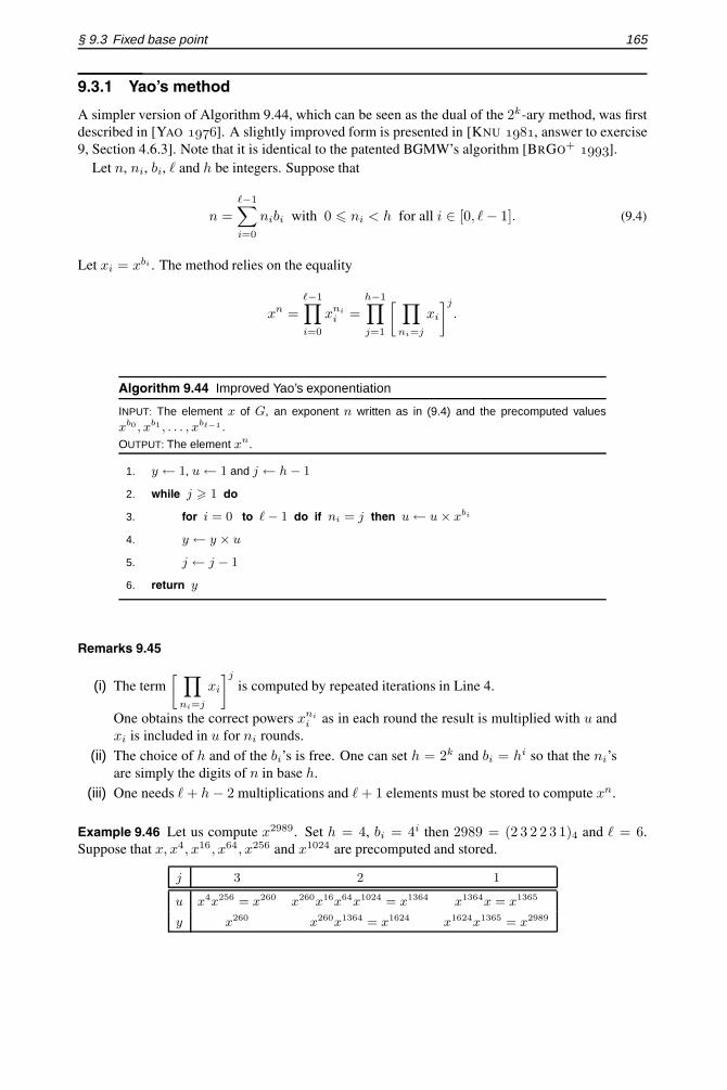
Example 9.46 Let us compute x2989. Set h = 4, bi = 4i then 2989 = (2 3 2 2 3 1)4 and = 6.Suppose that x, x4, x16, x64, x256 and x1024 are precomputed and stored.

j 3 2 1

u x4x256 = x260 x260x16x64x1024 = x1364 x1364x = x1365

y x260 x260x1364 = x1624 x1624x1365 = x2989


9.3.2 Euclidean method

The Euclidean method was first introduced in [ROO 1995], see also [SEM 1983]. Algorithm 9.47computes xn generalizing a method to compute the double exponentiation xn0

0 xn11 discussed by

Bergeron et al. [BEBE+ 1989] which is similar to the technique introduced in Section 9.2.2 to findshort addition chains. The idea is to recursively use the equality

xn00 xn1

1 = (x0xq1)

n0 × x(n1 mod n0)1 where q = �n1/n0�.

Algorithm 9.47 Euclidean exponentiation

INPUT: The element x of G, an exponent n as in (9.4) and the precomputed values x0 =xb0 , x1 = xb1 , . . . , x�−1 = xb�−1 .


1. while true do

2. Find M such that nM � ni for all i ∈ [0, � − 1]

3. Find N �= M such that nN � ni for all i ∈ [0, � − 1], i �= M

4. if nN �= 0 then

5. q ← �nM/nN�, xN ← xMq × xN and nM ← nM mod nN

6. else break

7. return xnMM

Example 9.48 Take the same exponent 2989 = (2 3 2 2 3 1)4 and let us evaluate x2989.

n5 n4 n3 n2 n1 n0 M N q x5 x4 x3 x2 x1 x0

— — — — — — — — — x1024 x256 x64 x16 x4 x

2 3 2 2 3 1 4 1 1 x1024 x256 x64 x16 x260 x

2 0 2 2 3 1 1 2 1 x1024 x256 x64 x276 x260 x

2 0 2 2 1 1 5 3 1 x1024 x256 x1088 x276 x260 x

0 0 2 2 1 1 3 2 1 x1024 x256 x1088 x1364 x260 x

0 0 0 2 1 1 2 1 2 x1024 x256 x1088 x1364 x2988 x

0 0 0 0 1 1 1 0 1 x1024 x256 x1088 x1364 x2988 x2989

0 0 0 0 0 1 0 1 — x1024 x256 x1088 x1364 x2988 x2989

9.3.3 Fixed-base comb method

This algorithm is a special case of Pippenger’s algorithm [BER 2002, PIP 1979, PIP 1980]. It is alsooften referred to as Lim–Lee method [LILE 1994]. It is essentially a special case of Algorithm 9.23where the different base points are in fact distinct powers of a single base. Suppose that n =(n�−1 . . . n0)2. Select an integer h ∈ [1, ]. Let a = �/h� and choose v ∈ [1, a]. Let r = �a/v�and write the ni’s in an array with h rows and a columns as below (pad the representation of n withzeroes if necessary)

§ 9.3 Fixed base point 167

a − 1 · · · 1 0na−1 · · · n1 n0

n2a−1 · · · na+1 na

......

......

nah−1 · · · nah−a+1 nah−a

For each s, the column number s can be read as the binary representation of an integer denoted byI(s). For example the last column I(0) is the binary representation of I(0) = (nah−a . . . nan0)2.The algorithm relies on the following equality

xn =r−1∏k=0

⎛⎝v−1∏

j=0

G[j, I(jr + k)]

⎞⎠

2k

where

G[j, i] =

(h−1∏s=0

xis2as

)2jr

for j ∈ [0, v − 1] and i = (ih−1 . . . i0)2 ∈ [0, 2h − 1].

Algorithm 9.49 Fixed-base comb exponentiation

INPUT: The element x of G and an exponent n. Let h, a, v, r and G[j, i] be as above.


1. y ← 1 and k ← r − 1

2. for k = r − 1 down to 0 do

3. y ← y2

4. for j = v − 1 down to 0 do

5. I ←Ph−1s=0 nas+jr+k2s [I = I(jr + k)]

6. y ← y × G[j, I ]

7. return y

Example 9.50 Once again, let us compute x2989. Set h = 3 and v = 2 so that a = 4 = rv, hencer = 2. Form the following array from the digits of 2989 = (101110101101)2

s 3 2 1 0

ns . . . n0 1 1 0 1na+s . . . na 1 0 1 0

n2a+s . . . n2a 1 0 1 1I(s) 7 1 6 5

The precomputed values are

i 0 1 2 3 4 5 6 7

G[0, i] 1 x x16 xx16 x256 xx256 x16x256 xx16x256

G[1, i] 1 x4 x64 x4x64 x1024 x4x1024 x64x1024 x4x64x1024


The algorithm proceeds as follows

k 1 1 1 0 0 0

j — 1 0 — 1 0

jr + k — 3 1 — 2 0

I — 7 6 — 1 5

G[j, I ] — x1092 x272 — x4 x257

y 1 x1092 x1364 x2728 x2732 x2989

Remarks 9.51

(i) One needs at most a + r − 2 multiplications and v(2h − 1) precomputed values. Ifsquarings can be achieved efficiently or “on the fly” (for example in finite fields of evencharacteristic represented through normal bases, see Section 11.2.1.c), only 2h−1 valuesmust be stored.

(ii) The adaptation of this method to larger base representations or signed representationssuch as the non-adjacent form is straightforward.

Exponentiation - koclab.cs.ucsb.edu

Documents

Transcript of Exponentiation - koclab.cs.ucsb.edu