Exponential Families Classification and Novelty …vishy/talks/Exponential.pdfparametric estimation...
50
S.V.N. “Vishy” Vishwanathan: Exponential Families, Page 1 Exponential Families Classification and Novelty Detection S.V.N. “Vishy” Vishwanathan [email protected] National ICT Australia and Australian National University Thanks to Alex Smola, Thomas Hofmann and Stéphane Canu
Transcript of Exponential Families Classification and Novelty …vishy/talks/Exponential.pdfparametric estimation...

S.V.N. “Vishy” Vishwanathan: Exponential Families, Page 1
Exponential FamiliesClassification and Novelty Detection
S.V.N. “Vishy” Vishwanathan
[email protected]://web.rsise.anu.edu.au/~vishy
National ICT Australiaand
Australian National University
Thanks to Alex Smola, Thomas Hofmann and StéphaneCanu

Overview
S.V.N. “Vishy” Vishwanathan: Exponential Families, Page 2
Review of Exponential Family
Log Partition FunctionConditional DensitiesMissing Variables
Maximum Likelihood Estimation
MAP Estimation
Gaussian Processes and the Normal PriorNovelty DetectionLarge Margin Classifiers
Graphical Models
Hammersley Clifford TheoremConditional Random Fields

Machine Learning
S.V.N. “Vishy” Vishwanathan: Exponential Families, Page 3
Data:Pairs of observations (xi, yi)
Underlying distribution P(x, y)
Examples (blood status, cancer), (transactions, fraud)
Task:Find a function f (x) which predicts y given x
The function f (x) must generalize well

Exponential Family
S.V.N. “Vishy” Vishwanathan: Exponential Families, Page 4
Basic Equation:We will use:
p(x; θ) = p0(x) exp(〈φ(x), θ〉 − g(θ))
Why?Dense in space of densities (L∞ sense)We can use 〈·, ·〉H where H is a RKHSConditional models and graphical models
Where is the Catch?The log-partition function
g(θ) = log
∫X
exp(〈φ(x), θ〉) dx
is difficult to compute

Log-Partition Function
S.V.N. “Vishy” Vishwanathan: Exponential Families, Page 5
Basic Equation:To ensure density integrates to 1
g(θ) = log
∫X
exp(〈φ(x), θ〉) dx
Domain X might be large (computing integral is painful)
Moment Generating Function:Derivatives of g(θ) generate moments of φ(x)
∂θg(θ) = Ep(x;θ) [φ(x)]
∂2θg(θ) = Varp(x;θ) [φ(x)]
Corollary:The log-partition function is convexIt is smooth and differentiable (C∞ function)

Some Examples
S.V.N. “Vishy” Vishwanathan: Exponential Families, Page 6
Bernoulli Distribution:Given by p(x;µ) = µx(1− µ)1−x
Exponential family form
p(x; θ) = exp(〈x, θ〉−log(1+exp(θ))) where θ = logµ
1− µ
Laplace Distribution:Model the decay of atoms by p(x; θ) = θ exp(〈−x, θ〉)In exponential family form
p(x; θ) = exp(〈−x, θ〉 − (− log θ))
Poisson Distribution:In exponential family form
p(x) = exp (〈x, θ〉 − log Γ(x + 1)− exp(θ))

Kernels
S.V.N. “Vishy” Vishwanathan: Exponential Families, Page 7
Problem: We want to perform non-parametric estimation (i.e. withoutdesigning the sufficient statistics)
Idea 1: Map to a higher dimensionalfeature space via Φ : x → Φ(x) andsolve the problem there Replace ev-ery 〈x, x′〉 by 〈Φ(x),Φ(x′)〉
Idea 2: Instead of computing Φ(x) ex-plicitly use a kernel functionk(x, x′) := 〈Φ(x),Φ(x′)〉A large class of functions are admis-sible as kernels
Non-vectorial data can be handled ifwe can compute meaningful k(x, x′)

Unconditional Models
S.V.N. “Vishy” Vishwanathan: Exponential Families, Page 8
Likelihood of data:Data X := {x1, . . . ,xm} generated IIDLikelihood is given by
p(X; θ) =
m∏i=1
p(xi; θ) = exp
(m∑i=1
〈φ(xi), θ〉 −mg(θ)
)Maximum Likelihood:
We want to minimize the negative log-likelihood
minimizeθ
g(θ)−
⟨1
m
m∑i=1
φ(xi), θ
⟩
=⇒ E[φ(x)] =1
m
m∑i=1
φ(xi) =: µ

An Example
S.V.N. “Vishy” Vishwanathan: Exponential Families, Page 9
Estimate the decay constant of an atom:We model decay using Laplace distributionUsing exponential family notation
p(x; θ) = exp(〈−x, θ〉 − (− log θ))
Computing µ:Observe that φ(x) = −xAll we need to do is average over observed decay times!
Solving for Maximum Likelihood:The maximum likelihood condition yields
µ = ∂θg(θ) = ∂θ(− log θ) = −1
θ
This leads to θ = −1µ

Conditional Models
S.V.N. “Vishy” Vishwanathan: Exponential Families, Page 10
Why Conditional Models?
We are given (xi, yi) pairsGiven a new data point we want to predict its label yWe don’t want to waste modeling effort on x
Conditional Exponential Family:
Assume p(y|x; θ) is a member of the exponential family
p(y|x; θ) = exp(〈φ(x, y), θ〉 − g(θ|x))
g(θ|x) = log
∫Y
exp(〈φ(x, y), θ〉 d y
The Task Ahead:
Estimate parameter θ and compute g(θ|x))
Handling Missing Variables
S.V.N. “Vishy” Vishwanathan: Exponential Families, Page 11
Partially Observed Data:
For partially observed data
p(xu, y|xo; θ) = exp (〈φ(xo,xu, y), θ〉 − g(θ|xo)) .The Density:
Integrate out unobserved part
p(y|xo; θ) =
∫Xu
exp (〈φ(xo,xu, y), θ〉 − g(θ|xo)) dxu
= exp(g(θ|xo, y)− g(θ|xo))

Overview
S.V.N. “Vishy” Vishwanathan: Exponential Families, Page 12
Review of Exponential Family
Log Partition FunctionConditional DensitiesMissing Variables
Maximum Likelihood Estimation
MAP Estimation
Gaussian Processes and the Normal PriorNovelty DetectionLarge Margin Classifiers
Graphical Models
Hammersley Clifford TheoremConditional Random Fields

Max-Likelihood Estimation
S.V.N. “Vishy” Vishwanathan: Exponential Families, Page 13
Observe Data:Data X = {(xi, yi)} drawn from distribution p(x, y|θ)
Compute Likelihood:Since data is assumed IID
log p(y|X; θ) =
m∑i=1
log p(yi|xi; θ)
Maximize it:Take the negative log and minimize, which leads to
Ep(y|x;θ)[φ(x, y)] =1
m
m∑i=1
φ(xi, yi)
This can be solved analytically or by Newton’s method.

Overview
S.V.N. “Vishy” Vishwanathan: Exponential Families, Page 14
Review of Exponential Family
Log Partition FunctionConditional DensitiesMissing Variables
Maximum Likelihood Estimation
MAP Estimation
Gaussian Processes and the Normal PriorNovelty DetectionLarge Margin Classifiers
Graphical Models
Hammersley Clifford TheoremConditional Random Fields

MAP Estimation
S.V.N. “Vishy” Vishwanathan: Exponential Families, Page 15
A True Bayesian:We assume that θ is a random variableAlso assume a prior (belief) over θ
The Normal Prior:We assume θ ∼ N(0, σ2)
The posterior (Bayes rule)
p(θ|X, y) ∝ exp
(m∑i=1
〈φ(xi, y), θ〉 − g(θ|x)− 1
2σ2‖θ‖2
)The Solution:
By setting ∂θ − log p(θ|X, y) = 0 we get
Ep(y|x;θ)[φ(x, y)] =1
m
∑φ(xi, yi)−
θ
mσ2

Gaussian Processes
S.V.N. “Vishy” Vishwanathan: Exponential Families, Page 16
Key Idea:Let t : X → R be a stochastic processFix any {x1, . . . ,xm}For a GP {t(x1), . . . , t(xm)} are jointly normal
Parameters of a GP:Mean
µ(x) := E[t(x)]
Covariance function (kernel)
k(x,x′) := Cov(t(x), t(x′))
Simplifying Assumption:Mean µ(x) = 0
We know the form of k(x,x′)

Our Model and GP
S.V.N. “Vishy” Vishwanathan: Exponential Families, Page 17
Key Idea:Let θ ∼ N(0, σ2)
Then log p(y|x; θ) + g(θ|x) is a GP
Why?:Observe that log p(y|x; θ) + g(θ|x) = 〈φ(x, y), θ〉Hence it is normally distributedThe mean Eθ[〈φ(x, y), θ〉] = 0
The covariance function
k((x, y), (x′, y)) = σ2〈φ(x, y), φ(x′, y′)〉Observations:
Kernel can depend on both x and yExtensions to multi-class problems possibleIf y has structure we can exploit it

Representer Theorem
S.V.N. “Vishy” Vishwanathan: Exponential Families, Page 18
Optimization Problem:The MAP estimate solves
argminθ
1
2σ2||θ||2 +
m∑i=1
g(θ|xi)− 〈φ(xi, yi), θ〉
Representer Theorem:By the representer theorem
θ =
m∑i=1
∑y∈Y
αiyφ(xi, yi)
Observations:If |Y | is large we are in troubleFor binary classification we will use φ(x, y) = yφ(x)

GP and Missing Variables
S.V.N. “Vishy” Vishwanathan: Exponential Families, Page 19
Partially Observed Data:
Plug in density into MAP estimate
minimize
m∑i=1
[g(θ|xoi )− g(θ|xoi , yi)] +1
2σ2‖θ‖2
Can of Worms?
Optimization problem is no longer convexWe will come back to this . . .

Conjugate Priors
S.V.N. “Vishy” Vishwanathan: Exponential Families, Page 20
Problems with Normal Prior:Posterior looks different from priorMany MLE algorithms may not work
Idea:What if the prior looked like additional data
p(θ|X) ∼ p(X |θ)For exponential families set
p(θ|a) ∝ exp(〈m0a, θ〉 −m0g(θ))
The Posterior:Now looks like
p(θ|X) ∝ exp
((m +m0)
(⟨mµ +m0a
m +m0, θ
⟩− g(θ)
))

Optimization Problems
S.V.N. “Vishy” Vishwanathan: Exponential Families, Page 21
Maximum Likelihood:
minimizeθ
m∑i=1
g(θ)− 〈φ(xi), θ〉 =⇒ ∂θg(θ) =1
m
m∑i=1
φ(xi)
Normal Prior:
minimizeθ
m∑i=1
g(θ)− 〈φ(xi), θ〉 +1
2σ2‖θ‖2
Conjugate Prior:
minimizeθ
m∑i=1
g(θ)− 〈φ(xi), θ〉 +m0g(θ)−m0 〈a, θ〉
equivalently solve ∂θg(θ) =1
m +m0
m∑i=1
φ(xi) +m0
m +m0a

Novelty Detection
S.V.N. “Vishy” Vishwanathan: Exponential Families, Page 22
Key Idea:We estimate p(x |θ) based on {xi}All xi with p(xi |θ) < p0 are novel
Tightening the Belt:Don’t waste modeling effort on high density regionsOnly shape of p(x |θ) is important
The Solution:Estimate
min
(p(xi |θ)p0
, 1
)We use p0 = exp(ρ− g(θ))
Helps get rid of pesky g(θ) term

Novelty Detection
S.V.N. “Vishy” Vishwanathan: Exponential Families, Page 23

Optimization Problem
S.V.N. “Vishy” Vishwanathan: Exponential Families, Page 24
Exponential Family:Using the iid assumption our objective function is
argmaxθ
m∏i=1
min
(p(xi |θ)p0
, 1
)p(θ)
The Final Form:If we assume a normal prior and use log likelihoods
argminθ
m∑i=1
max(ρ− 〈φ(xi), θ〉 , 0) +1
2σ2||θ||2
Exactly the problem solved by the Single class SVM!
The ν-Trick:Assume p(ρ) ∝ exp(νmρ)

Odds Ratio
S.V.N. “Vishy” Vishwanathan: Exponential Families, Page 25
Basic Idea:In OCR classification 0 and 8 are frequently confusedDigits like 0 and 1 are generally well classifiedWorst confused class is a measure of margin
The Solution:If we consider the ratio
R(x, y, θ) = logp(y|x, θ)
maxy 6=y′ p(y′|x, θ)Measure of confusion with the next best classWe can interpret this as the margin
The Consequences:SVM like large margin classifiers are special casesExtensions to multi-class setting natural
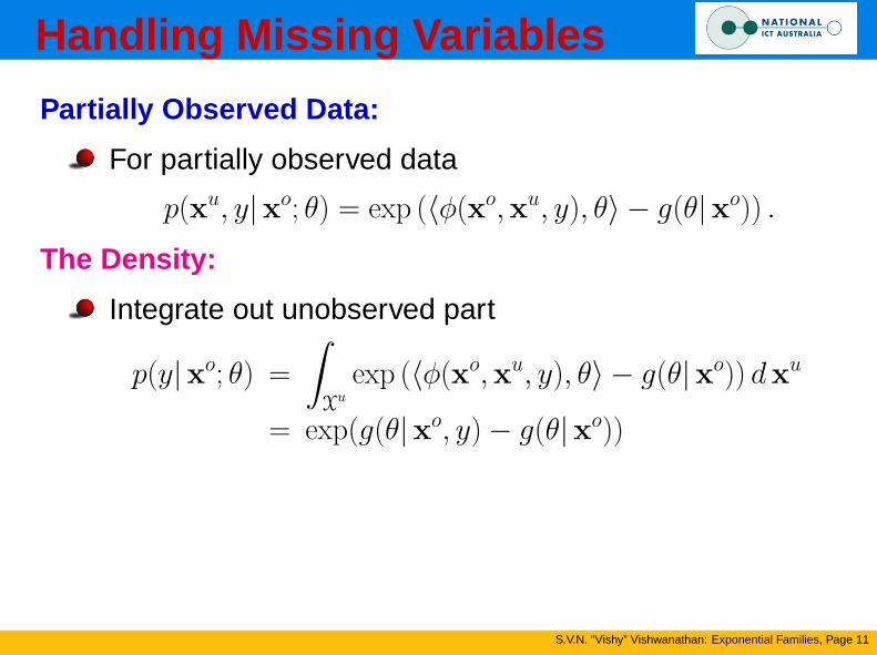
Multiclass SVM
S.V.N. “Vishy” Vishwanathan: Exponential Families, Page 26
A Problem:Three classes {1, 2, 3}Two densities {0.3, 0.3, 0.4} and {0.1, 0.5, 0.4}Class 3 has same likelihood in both casesIt is misclassified in the second case!
Odds Ratio Loss:The log odds ratio behaves like a margin
R(x, y, θ) = logp(y|x, θ)
maxy 6=y′ p(y′|x, θ)= 〈φ(x, y), θ〉 −max
y 6=y′〈φ(x, y′), θ〉
Generalized hinge loss
c(x, y, θ) := max(1−R(x, y, θ), 0)

Multiclass SVM - II
S.V.N. “Vishy” Vishwanathan: Exponential Families, Page 27
Optimization Problem:
We solve
minimize 12||θ||
2
s.t. R(xi, yi, θ) ≥ 1
Binary SVM:
Set φ(x, y) = y2φ(x)
Then R(x, y, θ) = y 〈φ(x), θ〉We now solve
minimize 12||θ||
2
s.t. yi 〈φ(xi), θ〉 ≥ 1
This is exactly the hard margin binary SVM!

Optimal Separating Hyperplane
S.V.N. “Vishy” Vishwanathan: Exponential Families, Page 28
Minimize1
2‖θ‖2 subject to yi〈θ,xi〉 ≥ 1 for all i
Odds Ratio and Missing Vars
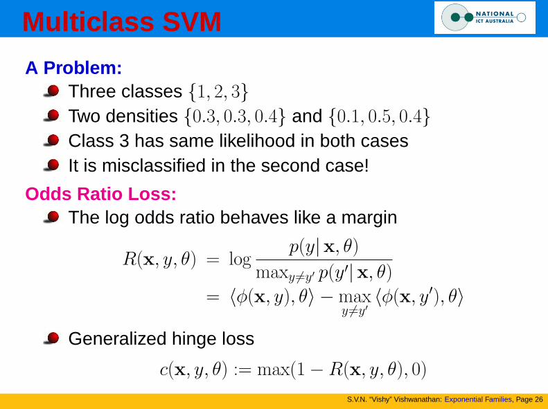
S.V.N. “Vishy” Vishwanathan: Exponential Families, Page 29
Log Odds Ratio:From definition of p(y|xo; θ) and R(x, y, θ):
R(x, y, θ) = g(θ|xo, y)−maxy′ 6=y
g(θ|xo, y′)
Expensive to compute!
The Optimization Problem:We now have to solve
minimize 12||θ||
2
s.t. g(θ|xo, y)−maxy′ 6=y g(θ|xo, y′) ≥ 1
The Challenge:Constraints are not convexClever sampling techniques required

Soft Margin SVM’s
S.V.N. “Vishy” Vishwanathan: Exponential Families, Page 30
Slack Variables:Data might not be linearly separable in feature spaceTo avoid over-fitting ignore noisy pointsWe modify the optimization problem
min 12||θ||
2 + C∑
i ξis.t.R(xi, yi, θ) ≥ 1− ξi ξi ≥ 0
Upper Bound on Error:If we define
ξi(θ) = max{0, 1−R(xi, yi, θ)}then
1
m
m∑i=1
ξi(θ) ≥1
m
m∑i=1
δ(yi, sign(logR(xi, yi, θ)))

Another Formulation
S.V.N. “Vishy” Vishwanathan: Exponential Families, Page 31
Slack Variables:We include a slack term for every linear constraintThe optimization problem becomes
min 12||θ||
2 + C∑
i
∑y 6=yi
ξiys.t.〈φ(xi, yi)− φ(xi, y), θ〉 ≥ 1− ξiy ξiy ≥ 0
Upper Bound on Ranking Error:Now we can write a bound
1
m
m∑i=1
ξiy(θ) ≥1
m
m∑i=1
|{y 6= yi : 〈φ(xi, y), θ〉 ≥ 〈φ(xi, yi), θ〉}|
Comments:More constraints =⇒ harder problem to solveSolution might not be sparse!

A Laundry List
S.V.N. “Vishy” Vishwanathan: Exponential Families, Page 32
Gaussian Process:
minimize
m∑i=1
[g(θ|xoi )− g(θ|xoi , yi)] +1
2σ2‖θ‖2.
SVM with Slack:
minimize1
2σ2‖θ‖2 +
m∑i=1
ξi
s.t. 1− ξi − g(θ|xoi , yi) + maxy 6=yi
g(θ|xoi , y) ≤ 0, and − ξi ≤ 0
Novelty Detection:
minimize 12σ2‖θ‖2 +
∑mi=1 ξi
s.t. ρ− ξi − g(θ|xo) ≤ 0 and − ξi ≤ 0

Constrained CCCP
S.V.N. “Vishy” Vishwanathan: Exponential Families, Page 33
The Problem:Suppose we want to solve
minimize f0(x)− g0(x)
s.t. fi(x)− gi(x) ≤ ci
Both fi and gi are convex for all i
The Basic Idea:Replace gi by a linear approximationSolve the new convex problemRepeat until convergence
Challenges:What is a good linear approximation?We use first order Taylor approximationRates of convergence?

Universal Density Estimators
S.V.N. “Vishy” Vishwanathan: Exponential Families, Page 34
Setting:Let X be a measurable set and k : X×X → R a kernelLet f (·) = 〈φ(·), θ〉H and f (x) = 〈f (·), k(·,x)〉HThe set of continuous and bounded densities on X be P
Furthermore let H be dense in C0(X)
Universal Density Estimators:The densities pf(x) := exp(f (x)− gf(θ)) are dense in P
Proof Sketch:Find a f (x) close to given p(x)
Show that∫
Xexp(f (x)) dx is bounded
It follows that | log pf(x)− log p(x)| is smallHence conclude that |pf(x)− p(x)| is small

Graphical Models
S.V.N. “Vishy” Vishwanathan: Exponential Families, Page 35
Basic Idea:x,x′ are conditionally independent given c, if
p(x,x′ |c) = p(x |c)p(x′ |c)This information might be known in advanceCan simplify distributions significantly
Markov Network:A graph G(V,E) with vertices V and edges EEach node of G represents a random variableEach subgraph of G is a subset of random variablesSubsets xS,xS ′ are conditionally independent given xC ifremoving the vertices C from G decomposes the graphinto disjoint subsets containing S, S ′.

Conditional Independence
S.V.N. “Vishy” Vishwanathan: Exponential Families, Page 36

Maximal Cliques
S.V.N. “Vishy” Vishwanathan: Exponential Families, Page 37
Definition:Maximally connected subgraph of a graph
Why are they Useful?Allow us to specify dependencies naturallyGraph algorithms can be used for inferenceHammersley Clifford Theorem

Hammersley Clifford Theorem
S.V.N. “Vishy” Vishwanathan: Exponential Families, Page 38
Theorem:If G encodes conditional independence assumptions
p(x) =1
Zexp
(∑c∈C
ψc(xc)
)Exponential Family:
Can apply decomposition to the exponential familyThe vector φ(x) decomposes as
φ(x) = (. . . , φc(xc), . . .)
Kernel Function:The kernel now looks like
k(x,x′) = 〈φ(x), φ(x′)〉 =∑c
〈φc(xc), φc(x′c)〉 =∑c
k(x,x′)

Proof
S.V.N. “Vishy” Vishwanathan: Exponential Families, Page 39
Step 1: Obtain linear functionalCombine exponential family with CH theorem:
〈Φ(x), θ〉 =∑c∈C
ψc(xc)− logZ + g(θ) for all x, θ
Step 2: Orthonormal basis in θSwallow Z and g(θ)Expand using an orthonormal basis
〈Φ(x), ei〉 =∑c∈C
ηic(xc) for some ηic(xc)

Proof contd . . .
S.V.N. “Vishy” Vishwanathan: Exponential Families, Page 40
Step 3: Reconstruct sufficient statisticsSince
Φc(xc) := (η1c (xc), η
2c (xc), . . .)
we can write
〈Φ(x), θ〉 =∑c∈C
∑i
θiΦic(xc)

Example: Normal Distribution
S.V.N. “Vishy” Vishwanathan: Exponential Families, Page 41
Density:
p(x |θ) = exp
n∑i=1
xi θ1i +
n∑i,j=1
xi xj θ2ij − g(θ)
Here θ2 = Σ−1, is the inverse covariance matrix. We havethat (Σ−1)[ij] 6= 0 only if (i, j) share an edge.

Example: Gaussian Distribution
S.V.N. “Vishy” Vishwanathan: Exponential Families, Page 42
Sufficient Statistics:For Gaussian distribution φ(x) = (x,xx>)
Clifford Hammersley Theorem:φ(x) must decompose into subsets on max cliquesThe linear term trivial to decomposeAn edge in the graph G(V,E) implies couplingIf xi is connected by edge to xj then this implies coupling
Inverse Covariance Matrix:Inverse covariance matrix corresponds to xx>
Its sparsity mirrors G(V,E)
Sparse inverse kernel matrix corresponds to a graphicalmodel!

Conditional Random Fields
S.V.N. “Vishy” Vishwanathan: Exponential Families, Page 43
Cliques and Density:Cliques are (xt, yt), (xt,xt+1), and (yt, yt+1)
Drop cliques in (xt,xt+1): no effect on p(y|x, θ)
p(y|x, θ) = exp(∑
t
〈φxy(xt, yt), θxy,t〉 + 〈φyy(yt, yt+1), θyy,t〉+
〈φxx(xt,xt+1), θxx,t〉 − g(θ|x))
Computational Issues
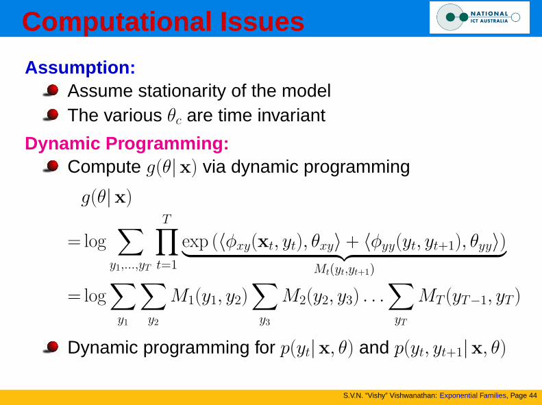
S.V.N. “Vishy” Vishwanathan: Exponential Families, Page 44
Assumption:Assume stationarity of the modelThe various θc are time invariant
Dynamic Programming:Compute g(θ|x) via dynamic programming
g(θ|x)
= log∑y1,...,yT
T∏t=1
exp (〈φxy(xt, yt), θxy〉 + 〈φyy(yt, yt+1), θyy〉)︸ ︷︷ ︸Mt(yt,yt+1)
= log∑y1
∑y2
M1(y1, y2)∑y3
M2(y2, y3) . . .∑yT
MT (yT−1, yT )
Dynamic programming for p(yt|x, θ) and p(yt, yt+1|x, θ)

Forward Backward Algorithm
S.V.N. “Vishy” Vishwanathan: Exponential Families, Page 45
Key Idea:
Store sum over all y1, . . . , yt−1 (forward pass) and overall yt+1, . . . , yT as intermediate valuesWe get those values for all positions t in one sweepExtend this to message passing (when we have trees)

Minimization
S.V.N. “Vishy” Vishwanathan: Exponential Families, Page 46
Objective Function:
− log p(θ|X, Y ) =
m∑i=1
−〈φ(xi, yi), θ〉 + g(θ|xi) +1
2σ2‖θ‖2 + c
∂θ − log p(θ|X, Y ) =
m∑i=1
−φ(xi, yi) + E [φ(xi, yi)|xi] +1
σ2θ
We only need E [φxy(xit, yit)|xi] and E[φyy(yit, yi(t+1))|xi
].
Kernel Trick
Conditional expectations Φ(xit, yit) pain to computeKernel trick works
〈φxy(x′t, y′t),E [φxy(xt, yt)|x]〉 = E [k((x′t, y′t), (xt, yt)|x]
Get p(yt|x, θ), p(yt, yt+1|x, θ) via dynamic programming

Subspace Representer Theorem
S.V.N. “Vishy” Vishwanathan: Exponential Families, Page 47
Representer Theorem:Solutions of the MAP problem are given by
θ ∈ span{φ(xi, y) for all y ∈ Y and 1 ≤ i ≤ n}
Big Problem:|Y | could be huge, e.g. for sequence annotation 2n.
Solution:
Exploit decomposition of φ(x, y) into sufficient statisticson cliques.Restriction of Y to cliques is much smaller.
θc ∈ span{φc(xci, yc) for all yc ∈ Yc and 1 ≤ i ≤ n}Rather than 2n we now get 2|c|.

Take Home Message
S.V.N. “Vishy” Vishwanathan: Exponential Families, Page 48
Exponential families are universal density estimators
Log partition functions are difficult to compute
Exponential families + Kernels =⇒ machine learning onsteroids
Gaussian Processes are MAP estimators in feature space
Novelty detection is density estimation in feature space
Support Vector Machines are also density estimators
Margins are the same as odds ratios
Graphical models and kernels can be married
Many interesting optimization problems

Questions?
S.V.N. “Vishy” Vishwanathan: Exponential Families, Page 49

Shameless Plug
S.V.N. “Vishy” Vishwanathan: Exponential Families, Page 50
We are hiring at NICTA
PhD, postdoc and visiting positions are availabe
Talk to me for more details