Exponential ﬁelds formulation for WMR...

Applied Bionics and Biomechanics 9 (2012) 375–397DOI 10.3233/ABB-2012-0054IOS Press

375

Exponential fields formulation for WMRnavigation

Edgar A. Martınez-Garcıaa,b,∗ and Rafael Torres-Cordobaa

aLaboratorio de Robotica, Institute of Engineering and Technology, Universidad Autonoma de Ciudad Juarez,Ciudad Juarez, Chihuahua, MexicobRobotica y Tecnologıa S. de R.L. Juarez, Chihuahua, Mexico

Abstract. In this manuscript, an autonomous navigation algorithm for wheeled mobile robots (WMR) operating in dynamicenvironments (indoors or structured outdoors) is formulated. The planning scheme is of critical importance for autonomousnavigational tasks in complex dynamic environments. In fast dynamic environments, path planning needs algorithms able tosense simultaneously a diversity of obstacles, and use such sensory information to improve real-time navigation control, whilemoving towards a desired goal destination. The framework tackles 4 issues: 1) Reformulation of the Social Force Model (SFM)adapted to WMR; 2) the cohesion of a general inertial scheme to represents motion in any coordinate system; 3) control of actuatorsrotational speed as a general model regardless kinematic restrictions; 4) assuming detection of features (obstacles/goals), adaptivenumeric weights are formulated to affect navigational exponential components. Simulation and experimental outdoors resultsare presented to show the feasibility of the proposed framework.

Keywords: Navigation, exponential components, dynamic model, directional fields

1. Introduction

Nowadays, service robotics is an exponentialgrowing area where human-robot interaction andcooperation play a critical roll in many task appli-cations. Most service robotics core-capabilities relyon navigation and mapping in dynamic environments.Regardless the sensing fashion, the system must feed-back to account for recognition capabilities. Servicerobots form a wide variety of applications, tasks, andmissions, requiring a wide range of capability issues:computational organization; smart algorithms; sensorscoordination and data fusion schemes; physical devices

∗Corresponding author: Edgar A. Martınez-Garcıa, Laboratoriode Robotica, Institute of Engineering and Technology, UniversidadAutonoma de Ciudad Juarez, Ciudad Juarez, Chihuahua, Mexico.E-mail: [email protected].

according to the tasks accomplishment; human-robot interaction; interfaces control; and real timeautonomous navigation capabilities. This manuscriptis centred on a general scheme to accomplish WMRautonomous navigation. During high speed naviga-tional tasks, robots face unexpected hazards that mustquickly be avoided, where the navigation controlalgorithm has strong relationship with the stabilityand manoeuvrability for the whole system. To avoidpotential crashes, reliable planning algorithms mustbe computationally efficient while considering impor-tant WMR and motion dynamic effects. In orderfor a WMR to have the required abilities to navi-gate autonomously, a wide variety of aspects mustbe integrated, among which include merging intelli-gent planners, distributed-based architecture systems,collective sensing capabilities, and all essentials that

1176-2322/12/$27.50 © 2012 – IOS Press and the authors. All rights reserved

376 E.A. Martınez-Garcıa and R. Torres-Cordoba / Exponential fields formulation for WMR navigation

depend on the kinematic models as means to createsophisticated control algorithms. Enhanced systemsproviding navigation safety will form a significant partof the market for intelligent automatic devices [24];because autonomous navigational developments suchas perception enhancement, route guidance, intelligenttracking control, and collision warning have the poten-tial to provide navigation much easier and speciallysafe [25]. The focus of the present work concerns amodel system for autonomous navigation, with capa-bilities that helps to avoid possible collisions directly.Direct avoidance includes features such as speed andsteer control that automatically slows the robot/vehicleif getting too close to any obstacle.

Social directional fields are algorithms that incre-mentally explore free space, while searching for asuitable path, acting as navigation planners applica-ble to a rich class of intelligent WMR to develop agreat variety of paths. The Social Force Model (SFM)was first reported by Helbing and Molnar [16] tosimulate pedestrians motion in crowd environments.They proposed a SFM analytically solved in termsof acceleration vectors that generalizes the influencesof a particle motion. However, the acceleration vectorcannot mathematically be easily integrated because adescriptive motion model is not given. Some worksdealing with potential fields treat the motion as a parti-cle, making this approach an applicable model to mostrolling-based locomotion systems, and do not includegeometry of motion constrained by the robot kinemat-ics. The concept of the SFM to simulate pedestriandynamics of forces interacting in crowd environmentshas some amazing similarities with gases and fluids-dynamic [38], which attracted interest for modellingvehicular traffic systems.

In the work of Gayle et al. [34], a similar approach tothe present context in using social potential fields arebuilt on physics-based reactive motion planning pre-sented with polyhedron-like soft bots (assuming point,point-like, circular or polygonal robot primitives);physics-based solve motion planning problems, andsocial potential fields exhibit various social behaviours,exhibiting relative easily and effectiveness at coordi-nating motion among multiple robots. However in itscontext it did not consider the variety of multi-bodykinematic descriptions.

Shimoda et al. [17] proposed a potential field-based method for high speed navigation of unmannedground vehicles on uneven terrain, where local minimaand maxima problems were addressed with a simple

randomization technique. Kareem et al. [18] presenteda fuzzy potential field approach for mobile robotmotion planning using two fuzzy models for eachfield, repulsive and attractive respectively. Baronov[19] presented a reactive control law to navigate asingle sensor-enabled vehicle to ascend or descend ascalar potential field. Ren et al. [20] proposed a poten-tial function based on generalized sigmoid functionsconstructed from combinations of implicit primitivesor from sampled surface data. Chunyu et al. [21]addressed a reactive control design for point-massvehicles with limited sensor range to track targetswhile avoiding static and moving obstacles in a dynam-ically evolving environment. Enxiu Shi et al. [22]presented an analysis of the common problems foundin potential fields for mobile robot such as obstacleavoidance, local trap and vibrating, an evolutionarymethod for improving potential fields was proposed.Charifa and Bikdash [23] compared the behaviour ofseveral variants of artificial potential function methodswith emphasis on the quality of path geometry, andvelocity and acceleration profiles. Loizou and Kyri-akopolous [30] proposed a kinematic framework formodelling mobility of multiple robots that mathemati-cally combines heterogeneous locomotion constraintsfor control of the system.

Today’s vehicle-like robots have more complexfunctions with features of object detection and posi-tioning capabilities Stanek et al. [9], specially long-term navigational tasks Broggi et al. [8]. Numerouskinematic planners that compute the shortest manoeu-vring feasible path for vehicles explicitly consideringvehicle dynamics is found in Moriwaki and Tanaka[12]; and similarly Werling et al. [6] presented a searchfor an optimal path using dynamic simulations todetermine the traversable or cost of specific terrain seg-ments. Tychonevich et al. [7] presented a work basedon selecting a path that is ensured to be statically safe.Such approaches do not account for vehicle dynam-ics and speed. Other works on multi-layered plannersto achieve optimal navigation of high speed mobilerobots on outdoors using layered control has been pro-posed Iagnemma et al. [13], and Plaku et al. [11].High-level planning layers generate optimal desiredtrajectories as series of way-points, and low-level layerto guide the vehicle using potential fields. But optimalglobal trajectory generation must be off-line to com-pute a topographic model, and then dynamic obstaclesare not considered. Fuzzy genetic-based planners hasbeen develop to account for obstacles in terrain regions

E.A. Martınez-Garcıa and R. Torres-Cordoba / Exponential fields formulation for WMR navigation 377

to determine vehicle speed, or similar approaches torepresent traversable, or very cluttered environmentsSelekwa et al. [2]. Global trajectory planners that deter-mine traversable directly, use a search where first selecta series of “best”traversable paths, which are then fur-ther optimized to minimize travel time, but no consider-ation of detailed vehicle models exist Mann and shiller[14]. Artificial potential fields have long been success-fully employed for robot navigation to solve severalnavigation problem Masound [4]. To develop real-timeobstacle avoidance Huang et al. [1]; trajectory genera-tion Mora and Tornero [3]; dynamic control of mobilerobots with moving obstacles and goals Geand and Cui[15] and Selekwa et al. [2]; general robot path plan-ning applied to (non) holonomic platforms Goncalveset al. [5]; simulations on multiple robotic agents mov-ing guided by potential fields along urban intersectionslanes was presented in Teja et al. [10].

Our analysis regarding cited references summarizesthat directional fields are physics-based models gener-ally solvable equations of first and second order, withimplicit control in the model itself for high speeds.Many practical robotic navigation problems have beensuccessfully solved. Local minima and maxima hasbeen largely treated by the robotics community, andcurrently there exist a variety of available solutions.Directional fields are relatively easy to adapt in mul-tiple robotic systems, regardless, either functional orlocomotive robots heterogeneity. Directional fields areproved to have the path geometry quality if adjustmentsand algebraic restrictions are included (dependingon the task). They can be stated as reactive controllaws, having great flexibility to be adjusted to anykinematics structure. Some contributions are of prac-tical implementation, while some others are real-timeintractable, and definitely are off-line solutions. Ourcontribution research is another approach of direc-tional fields applied to mobile robotics; the SFM wasstated for other scientific applications (gas kineticsand crowd scenarios simulations). We are reformulat-ing this approach to be adapted to WMR for on-lineplanning with exponential-based distributions. Thismanuscript presents a framework that includes thekinematics and motion dynamics model in continuous-time merged with a general model that reformulatesthe SFM to solve the motion-planning problem. Thecontributions of the present work has the followingissues, the SFM is reformulated as a general velocity-based motion framework that expresses internal andexternal causes and effects of motion constrained to an

ideal and a maximal speeds control. The speed con-trol is based on a functional form of motors rotationalspeed rate, and the robot’s size to determine the vehicleyaw speed, and with such basis the actual and posteriorposition vectors are formulated. The combined schemeallows any forward kinematics, since it depends onthe locomotion robot’s design, and a weighting fac-tor yielded from multiple sensing features. Using themotion dynamic equations, motion is no longer purelygeometric because directions are computed on accel-eration components and unit vectors.

This manuscript is organized as follows. In section 2,a description of the problem to be solved is presented.The section 3 introduces the robot main control lawmodel. Section 4 details the general social acceler-ations model, and the mechanism to yield adaptivenumeric weights to affect the robot steering navigationfunction. Section 5 presents the derivation of a modelto describe the robot motion in either local or globalframework. Further, section 6 concerns the derivationof a motion dynamics model that describes Newton’slaw of motion. We describe an equilibrium conditionbetween causes and effects of motion in any inertialframe. Section 7 describes in detail the formulationto infer the actual and next robot position vector. Sec-tion 8 presents the directional fields navigation schemethat is comprised of exponential accelerative vectorcomponents. Section 9 discusses the simulation andexperimental results. Finally, section 10 summarizesthe work conclusions.

2. Problem definition

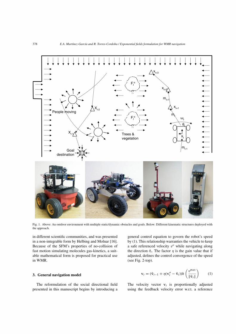
We state a traditional navigation problem as illus-trated by Fig. 1. A WMR µ with fixed inertial framexµt = (x, y)T , heading to θt , and passing through asequence of local goals at xt , each with direction mt ;while leading the robot toward a goal destination γ .The Cartesian distance between two points is gener-ally defined by the norm of their geometric difference‖�δµα‖ = ‖xµt − xαt ‖ (distance between robot µ andobstacle αt). Goals are established to exert attractiveaccelerative fields Fγt which easily conduct the robot.Likewise, detected obstacles α exert repulsive accele-rative fields Fαt . Both types of fields, in combinationform an enriched directional map. One of the prob-lems in this work is how to reformulate the SFM as areliable navigation solution for WMR. The SFM wasoriginally presented to solve other scientific problems


People moving

Goal destination

Trees & vegetation

Ft

Ft

xt

mt-1

t

t

mt

xt+1

xt+2

xt+3

mt+1

Xt-1

Xt-2

Fig. 1. Above: An outdoor environment with multiple static/dynamic obstacles and goals. Below: Different kinematic structures deployed withthe approach.

in different scientific communities, and was presentedin a non-integrable form by Helbing and Molnar [16].Because of the SFM’s properties of no-collision offast motion simulating molecules gas-kinetics, a suit-able mathematical form is proposed for practical usein WMR.

3. General navigation model

The reformulation of the social directional fieldpresented in this manuscript begins by introducing a

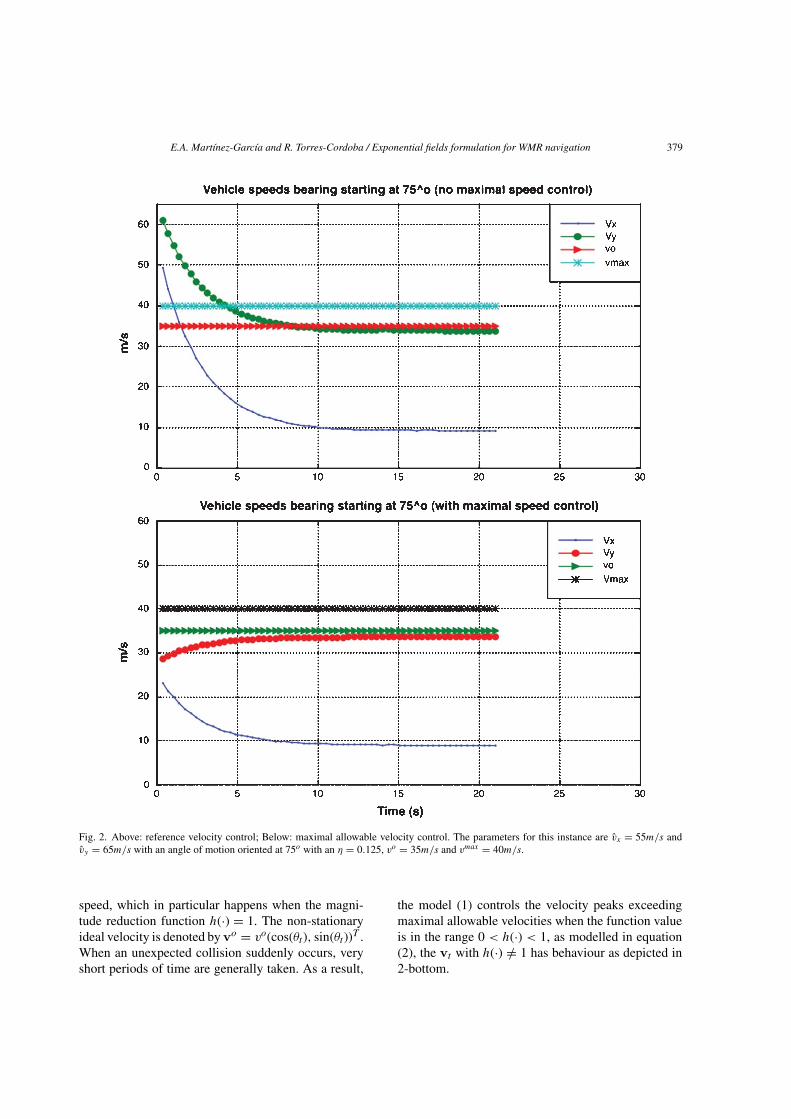
general control equation to govern the robot’s speedby (1). This relationship warranties the vehicle to keepa safe referenced velocity vo while navigating alongthe direction θt . The factor η is the gain value that ifadjusted, defines the control convergence of the speed(see Fig. 2-top).

vt = (vt−1 + η(vot − vt))h(vmax

‖vt‖)

(1)

The velocity vector vt is proportionally adjustedusing the feedback velocity error w.r.t. a reference


Fig. 2. Above: reference velocity control; Below: maximal allowable velocity control. The parameters for this instance are vx = 55m/s andvy = 65m/s with an angle of motion oriented at 75o with an η = 0.125, vo = 35m/s and vmax = 40m/s.

speed, which in particular happens when the magni-tude reduction function h(·) = 1. The non-stationaryideal velocity is denoted by vo = vo(cos(θt), sin(θt))T .When an unexpected collision suddenly occurs, veryshort periods of time are generally taken. As a result,

the model (1) controls the velocity peaks exceedingmaximal allowable velocities when the function valueis in the range 0 < h(·) < 1, as modelled in equation(2), the vt with h(·) /= 1 has behaviour as depicted in2-bottom.


h(vmax, ‖vt‖

) =

⎧⎪⎪⎨⎪⎪⎩

0, ‖vt‖ = 0

1, 0 < ‖vt‖ ≤ vmax

vmax

‖vt‖ , vmax < ‖vt‖(2)

The velocity model (1) recursively controls twoaspects; first, the real velocity fluctuating around theideal velocity vo magnitude; and second, removingdivergent magnitudes overpassing a maximal allow-able velocity value. The real velocity vector vt at actualtime t is defined in (3), the real velocity model in thiscontext will involves the motion causes, motion effects,and random fluctuations perturbing acceleration com-ponents. The real velocity vector vt is expressed interms of two global accelerative components that yielddvdt as in equation (3). One term is the social directional

field vector is Ft = (fx, fy)T expresses the internaland external causes of motion by Newton’s 2nd law ofmotion F/m withm = 1, affecting the WMR motion.The second termat = (ax, ay)T is the general accelera-tion representing accelerative behaviour for any inertialsystem (global aI , or local aR).

dvdt

= Ft − aIt (3)

4. Social field functions

Social field functions Ft stated in (3) as the gen-eral real motion model vt , expresses robot’s globalbehaviour involving dynamic causes of motion. Weencompass three causes of motion dynamics (sen-sors are deployed in the process for detection),next desired goals (an approach is presented by visualdetection in Fig. 3), obstacles position (LIDARs), andfinal goal destinations. Eq. (4) models the social direc-tional fields described in terms of global accelerationsFt . Cases of motion are internal (Fot ), and external (Fαtand Fγt ).

Ft = Fot +∑α

Fαt +∑γ

Fγt (4)

Since the robot’s navigation depends on sensor obser-vations, only sensor data feature are used as regions ofinterest to exert weighted navigation functions. Eachaccelerative force is defined with an adaptive numericweightw(mt , ft) yielded by the bearing location of thetargets (local goal destination, or obstacles) within thesensors field of view as defined in equation (5).

Ft = Fot +∑α

w(mt ,−fαt )fαt +∑γ

w(mt , fγt )fγt

(5)

The repulsive and attractive behaviour, which affectthe vehicle’s behaviour accentuate the magnitudes ofthe motion functions given in expressions (6) and (7),where �δµ = xαt − xµt is a distance vector between thepositions of a goal/obstacle and the actual vehicle µ,and the mt = (xµt+1 − xµt )/‖(xµt+1 − xµt )‖ is a unitvector expressing the direction towards a next desiredlocation xt+1. Thus, the weighting factorwt will affectthe repulsive acceleration behaviour according to,

Fαt (m, �δµα) = w(mt ,−fαt )f (�δµα) (6)

similarly the weighting factor will affect the attractiveacceleration by,

Fαt (m, �δµγ ) = w(mt , fγt )f (�δµγ ) (7)

The influence of the weight wt depends on how paral-lel the sensing direction φt of a goal/obstacle and theactual acceleration f are, as described in expression(8). If the actual orientation of the vector accelerationf is about the same as the actual vehicle desired ori-entation mt , then no change of direction is requiredfor the vehicle. It is expected that the orientation ofthe goal/obstacle sensed at bearing φt is approximatelyalong the direction of the next desired position. But, ifthe orientations of vectors mt and φt are different, thenit means that the horizontal component ft cosφ mustbe decreased by the vehicle yaw changes.

wt ={

1, mt · ft ≥ ‖ft‖ cos(φit)

λt, otherwise(8)

The influence of rotations that the vehicle must carryout is given by an influence term λt which is an aver-age of the fusion of all multi-sensory observations. Aswe established that the vehicle is instrumented with sndifferent sensor devices i. Thus, λt is valued within therange 0 ≤ λ ≤ 1 based on an effective angle of viewφt ,

λt = sin

(1

sn

∑i

φit

π

)(9)

Where sn is the total number of sensors involved inthe perception of the objective (goal/obstacle), and(φt)

sni are the angles at which each sensor i detected the

same objective. In fact, expression (9) defines a greater


Table 1Algorithm Robot’s sensor data

1: read-from-lidar( θt,xt)2: Zt=read-lidar(); Zt = {z1

t , . . . , zmt }

3: z = (φi, di)T ;4: xsit = (di cos(φi), di sin(φi))T

5: Xt = {xs1t , . . . ,xsmt }6: XI

t = R(θt) · xsit + xt7: return XI

t

numeric weight to objectives located nearly alongthe longitudinal vehicle’s axis (fixed-frame, defined at90o). Sensing modality for environment mapping is bydeploying a laser range finder. The important features,which the robot is able to perceive are very criticalbecause on this issue, the robot defines the numericweighting factors to impact significantly the naviga-tion functions. The Table 1 defines z as the vector ofa polar measurement (one point among the 681 of thelaser scan). Likewise, xsit defines the Cartesian repre-sentation of a point zi. The Table 1 directly returns asensor observation in a global Cartesian representationXIt .In outdoor experiments under natural light con-

ditions [35–37] the attractive areas xγt (middle-roadtriangles) and repulsive features xαt (line lanes cir-cles) were detected on-line using vision as depictedby the sequence of images of Fig. 3. The attrac-tive local goals (γ) are featuring the next desiredpositions {xγt ,xγt+1 . . . }. Line lanes regions representrepulsive objectives (α). Other feature points over

the horizon and/or dynamic and static obstacles areused for complementing localisation by monocularvisual odometry, which is out of the scope of thismanuscript.

5. Inertial frames motion

Definition of robot’s motion must be described inlocal/global Cartesian frames to represent accelerationmaps (Fig. 11). We define a generalised particle motionscheme, in which neither causes of motion, nor vehi-cle kinematic restrictions are regarded. Such scheme isuseful to model accelerative motion behaviour denotedby at , already described by eq. (3) to describe partof the real acceleration dv

dt . Let us consider the lin-ear velocity components of any vehicle-like robot withaveraged velocity vt . By defining the velocity vectorvRt = (vx, vy)T in the vehicle fixed-frame, the compo-nentsXY represent the 2D plane of motion and is givenby the expression (10),

vRt = vt

(cos(θt)

sin(θt)

)(10)

Where θt is the vehicle’s angle of motion w.r.t. robot’sinitial posture. By transforming the original vehiclefixed-frame using a transformation matrix R withrotation angle ψ between the robot’s frame, and theglobal system. The new expression for the global framebecomes as expressed by (11), which is the velocity

Fig. 3. Outdoor experiments using vision were realised to detect φi corresponding to γ and α. The triangles define attraction areas for theweighting function w(u, f γt ) to impact f γt (�δ).


0 5 10 15

a x (m

/s2)

t (sg)0 5 10 15

−0.1

−0.05

0

0.05

0.1

−0.1

−0.05

0

0.05

0.1

a y (m

/s2 )

t (sg)

0 5 10 15−100

−50

0

50

100

Ang

le

t (sg)

−0.02 0 0.02

−0.02

−0.01

0

0.01

0.02

Vx (m/S)

Vy

(m/s

)

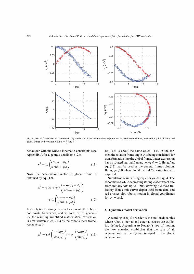
Fig. 4. Inertial frames descriptive model (12) yielded results of accelerations represented in two inertial frames, local frame (blue circles), andglobal frame (red crosses), with ψ = π

2 and θt .

behaviour without wheels kinematic constraints (seeAppendix A for algebraic details on (12)).

vIt = vt

(cos(θt + ψt)

sin(θt + ψt)

)(11)

Now, the acceleration vector in global frame isobtained by eq. (12),

aIt = vt(θt + ψt)

(− sin(θt + ψt)

cos(θt + ψt)

)

+ vt

(cos(θt + ψt)

sin(θt + ψt)

)(12)

Inversely transforming the acceleration into the robot’scoordinate framework, and without lost of general-ity, the resulting simplified mathematical expressionis now written in eq. (13) as the robot’s local frame,hence ψ = 0.

aRt = vtθ

(− sin(θt)

cos(θt)

)+ vt

(cos(θt)

sin(θt)

)(13)

Eq. (12) is about the same as eq. (13). In the for-mer, the rotation frame angleψ is being considered fortransformation into the global frame. Latter expressionhas no rotated inertial frames, henceψ = 0. Hereafter,eq. (12) may be used as the general frame solution.Being ψt /= 0 when global inertial Cartesian frame isrequired.

Simulation results using eq. (12) yields Fig. 4. Therobot moved while decreasing its angle at constant ratefrom initially 90o up to −50o, drawing a curved tra-jectory. Blue circle curves depict local frame data, andred crosses plot robot’s motion in global coordinatesfor ψt = π/2.

6. Dynamics model derivation

According to eq. (3), we derive the motion dynamicswhere robot’s internal and external causes are explic-itly defined. According to Newton’s law of motion,the next equation establishes that the sum of allaccelerations in the system is equal to the globalacceleration,


at = 1

m

∑i

2√fx2i + fy2

i ≡∑i

2√fx2i + fy2

i (14)

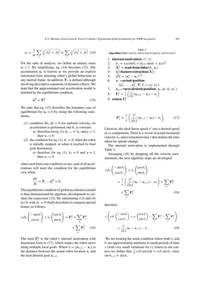
For the sake of analysis, we define an unitary massm = 1. By simplifying, eq. (14) becomes (15). Theacceleration at is known as we provide an explicitfunctional form denoting robot’s global behaviour inany inertial frame. In addition, Ft is defined althoughinvolving descriptive equations of dynamic effects. Westate that the approximated real acceleration model isdenoted by the equilibrium condition,

aRt = Fµt (15)

We state that eq. (15) describes the boundary case ofequilibrium for at = 0 by rising the following state-ments,

(1) condition dvt/dt = 0 for uniform velocity, noacceleration is performed and vt is constant.

a) therefore for eq. (1), vt−1 ≡ vt , andη = 1,then vt = 0

(2) the condition for eq. (1), vt = 0, when the robotis initially stopped, or when it reached its finalgoal destination.

a) therefore for eq. (1), vt = 0 and η = 1,then vt = 0

when such limit case condition occurs, sum of all accel-erations will meet the condition for the equilibriumcase when,

dvdt

= Ft − aRt = 0

The equilibrium condition of global accelerative modelis then demonstrated by algebraic development to val-idate the expression (15). By substituting (12) and (4)in (3) with ψt = 0 (both described in common inertialframe) as follows,

vtθt

(− sin θtcos θt

)+ vt

(cos θtsin θt

)= Fot +

∑α

Fαt

+∑γ

Fγt (16)

The term Fot is the robot’s internal motivation withfunctional form in (17), which makes the robot movealong multiple local goals. Where δ = ‖xt+1 − xt‖ isthe distance between the actual robot location xt andthe next desired goal xt+1.

Table 2Algorithm Directional field for internal motivation

1: internal-motivation( vo, τ)2: vt = vt(cos(θt + ψt), sin(θt + ψt))T

3: XIt = read-from-lidar(θt,xt)

4: xst=feature-extraction(XIt )

5: ‖�δ‖ = (xst − xt)1/2

6: xt =actual-position(ϕ1t , . . . , ϕ

nt ,W,L, r, x0, y0 )

7: xt+1=next-desired-position( xt , φi, θt, wt )

8: Fot = 1τ

(vo

‖�δ‖ (xt+1 − xt) − vt)

9: return Fot

Fot = 1

τ

(vo

‖�δt‖(xt+1 − xt) − vt

)(17)

Likewise, the ideal linear speed vo sets a desired speedin xy components. There is a vector of actual measuredvelocity vt , and a relaxation time τ that defines the timetaken for speeds change.

The internal motivation is implemented throughTable 2.

Arranging (16) by dropping off the velocity mea-surement, the next algebraic steps are developed

vtθt

(− sin θtcos θt

)+ vt

(cos θtsin θt

)

= 1

τ

(vo

‖�δt‖(xt − xt+1) − vt

)+∑α

Fαt

+∑γ

Fγt (18)

therefore,

τ

(vt θt

(− sin θt

cos θt

)+ vt

(cos θt

sin θt

)−∑α

Fαt −∑γ

Fγt

)

= vo

‖�δt‖(xt − xt+1) − vt (19)

We are treating the usual condition where both vt andθt are approximately uniforms in small periods of timeτ (with very small variations for τ), where in our con-text we define that

∫tvt θt sin θtdt ≈ vtθt sin θt , since

sin θt−1 ≈ sin θt .


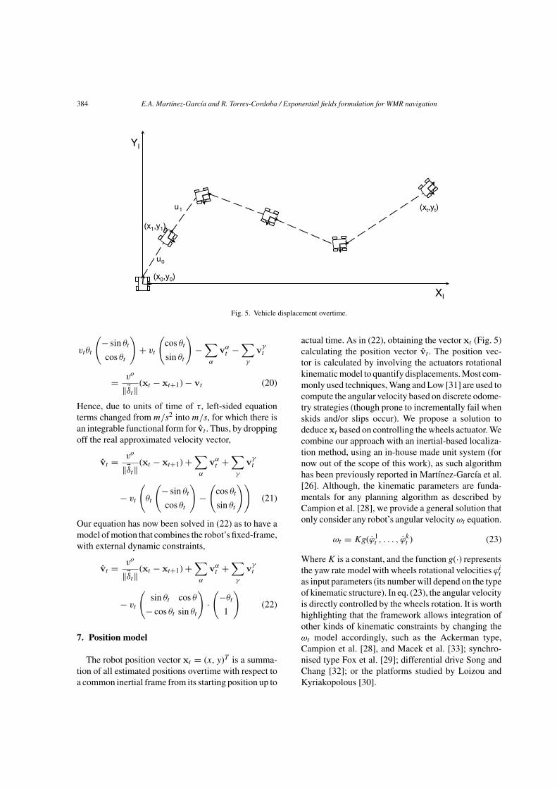
Fig. 5. Vehicle displacement overtime.

vtθt

(− sin θtcos θt

)+ vt

(cos θtsin θt

)−∑α

vαt −∑γ

vγt

= vo

‖�δt‖(xt − xt+1) − vt (20)

Hence, due to units of time of τ, left-sided equationterms changed from m/s2 into m/s, for which there isan integrable functional form for vt . Thus, by droppingoff the real approximated velocity vector,

vt = vo

‖�δt‖(xt − xt+1) +

∑α

vαt +∑γ

vγt

− vt

(θt

(− sin θtcos θt

)−(

cos θtsin θt

))(21)

Our equation has now been solved in (22) as to have amodel of motion that combines the robot’s fixed-frame,with external dynamic constraints,

vt = vo

‖�δt‖(xt − xt+1) +

∑α

vαt +∑γ

vγt

− vt

(sin θt cos θ

− cos θt sin θt

)·(

−θt1

)(22)

7. Position model

The robot position vector xt = (x, y)T is a summa-tion of all estimated positions overtime with respect toa common inertial frame from its starting position up to

actual time. As in (22), obtaining the vector xt (Fig. 5)calculating the position vector vt . The position vec-tor is calculated by involving the actuators rotationalkinematic model to quantify displacements. Most com-monly used techniques, Wang and Low [31] are used tocompute the angular velocity based on discrete odome-try strategies (though prone to incrementally fail whenskids and/or slips occur). We propose a solution todeduce xt based on controlling the wheels actuator. Wecombine our approach with an inertial-based localiza-tion method, using an in-house made unit system (fornow out of the scope of this work), as such algorithmhas been previously reported in Martınez-Garcıa et al.[26]. Although, the kinematic parameters are funda-mentals for any planning algorithm as described byCampion et al. [28], we provide a general solution thatonly consider any robot’s angular velocityωt equation.

ωt = Kg(ϕ1t , . . . , ϕ

kt ) (23)

WhereK is a constant, and the function g(·) representsthe yaw rate model with wheels rotational velocities ϕitas input parameters (its number will depend on the typeof kinematic structure). In eq. (23), the angular velocityis directly controlled by the wheels rotation. It is worthhighlighting that the framework allows integration ofother kinds of kinematic constraints by changing theωt model accordingly, such as the Ackerman type,Campion et al. [28], and Macek et al. [33]; synchro-nised type Fox et al. [29]; differential drive Song andChang [32]; or the platforms studied by Loizou andKyriakopolous [30].


Table 3Algorithm Actual robot position

1: actual-position ( ϕ1t , . . . , ϕ

nt , x0, y0 )

2: t = robot-actual-orientation(θ0,K, ϕ

1t , . . . , ϕ

nt )

3: θt = θ0 + t4: xt = (x0, y0)T + ∫

tv0

+ ∫tvtdt(cos θt, sin θt)T dt

5: return xt

The approach to infer xt and xt+1 is by quantify-ing the wheels angular displacement directly by thespeed drivers. We take advantage of the control hard-ware (motor drivers) which works under asymptoticfunctions (although a non-linear motor speed curvewill vary from product to product). A general relation-ship beetween actuator’s angular speed ϕt and a digitalcontrol variable �t is kinematically given by

ϕt(�) = (a

1 + e−��−µ ) − b (24)

Where a and b are constants that adjust the non-linearangular velocity behaviour curve, � is the constant offast asymptotic fall, � is a control digital word whichis associated with an angular speed given directly by auser program, and µ is the central value of the veloc-ity curve. By solving (24), we integrate the equationto obtain the next expression (25) en terms of wheelsinstantaneous angle of rotation,∫ b

a

ϕ(�)d� = ϕ(�) = (a− b)�

+ a

�ln(1 + e�(µ−�)) (25)

We synthesize the robot’s direction and deduce a for-mal position model equation as expressed in the vectorform by (26) with the k rotation velocities ϕit .

xt =(x0

y0

)+∫ tn

t0

(v0 +∫ tn

t1

vtdt

(cos(θ0 +K

∫ tg(ϕ1

t , . . . , ϕkt )dt

sin(θ0 +K∫ tg(ϕ1

t , . . . , ϕkt )dt

)dt)dt (26)

Inferring the robot’s actual position is synthesised inpseudo-code form by the algorithm 3. Nevertheless, theproblem of robot skid/slip is overcome by combiningwith the method reported in Martınez-Garcıa et al. [26]that deploys an in-house made inertial unit. It worksreasonable because yaw rates can directly be controlledby using low level commands. Thus, by simplifyingprevious expression,

t = K

∫ tn

t1

g(ϕ1t , . . . , ϕ

nt )dt (27)

Substituting (25) in (27) and algebraically solving,

t = K(

(a− b)�r + a

�ln(1 + e�(µ−�r))

−(a− b)�l + a

�ln(1 + e�(µ−�l))

)(28)

then,

t = K

((a− b)(�r −�l) + a

�ln

(1 + e�(µ−�r)

1 + e�(µ−�l)

))(29)

We assume similar approach as Fox et al. [29], wherea dynamic motion algorithm derived from the robot’sgeneral dynamics was presented. Hence, the actualposition vector is written as,

xtn =(x0

y0

)+∫ tn

t0

(v0 +∫ tn

t1

vtdt

(cos(θ0 + t)

sin(θ0 + t)

)dt)dt

(30)

The orientation θt is solved by integration w.r.t. thetime interval [t0, tn], in which wheels rotations arecontrolled rather than collecting absolute odome-try measurements (as commonly proposed by otherapproaches). Thus, reformulating the robot’s angle by

θt = θ0 +K

∫ t

t1

g(ϕ1t , . . . , ϕ

nt )dt (31)

and solving for the instantaneous angle,

θt = θ0 + t (32)

We assumed that the magnitude of the vehicle’sangular acceleration dω/dt at every control loop is

much smaller than the magnitude of the angular veloc-ity. The robot’s orientation algorithm is presented inTable 4, which obtains the actual robot’s angle. Theskidding and slipping aspects are treaten in Martınez-Garcıa et al. [27].

Arranging the actual position vector to be algorith-mically implemented in terms of the robot kinematic


Table 4Algorithm Robot’s actual orientation

1: robot-actual-orientation (θ0,K, ϕ1t , . . . , ϕ

nt )

2: Set constants �, a, b,�,µ

3: t = K(

(a− b)(�r −�l) + a�

ln 1+e�(µ−�r )

1+e�(µ−�l)

)4: θt = θ0 + t5: return θt

structure,

xt =(xt+1

yt+1

)�t + r

2g(ϕrt , . . . , ϕ

lt

)�t

(cos(θ0 + t)

sin(θ0 + t)

)

(33)

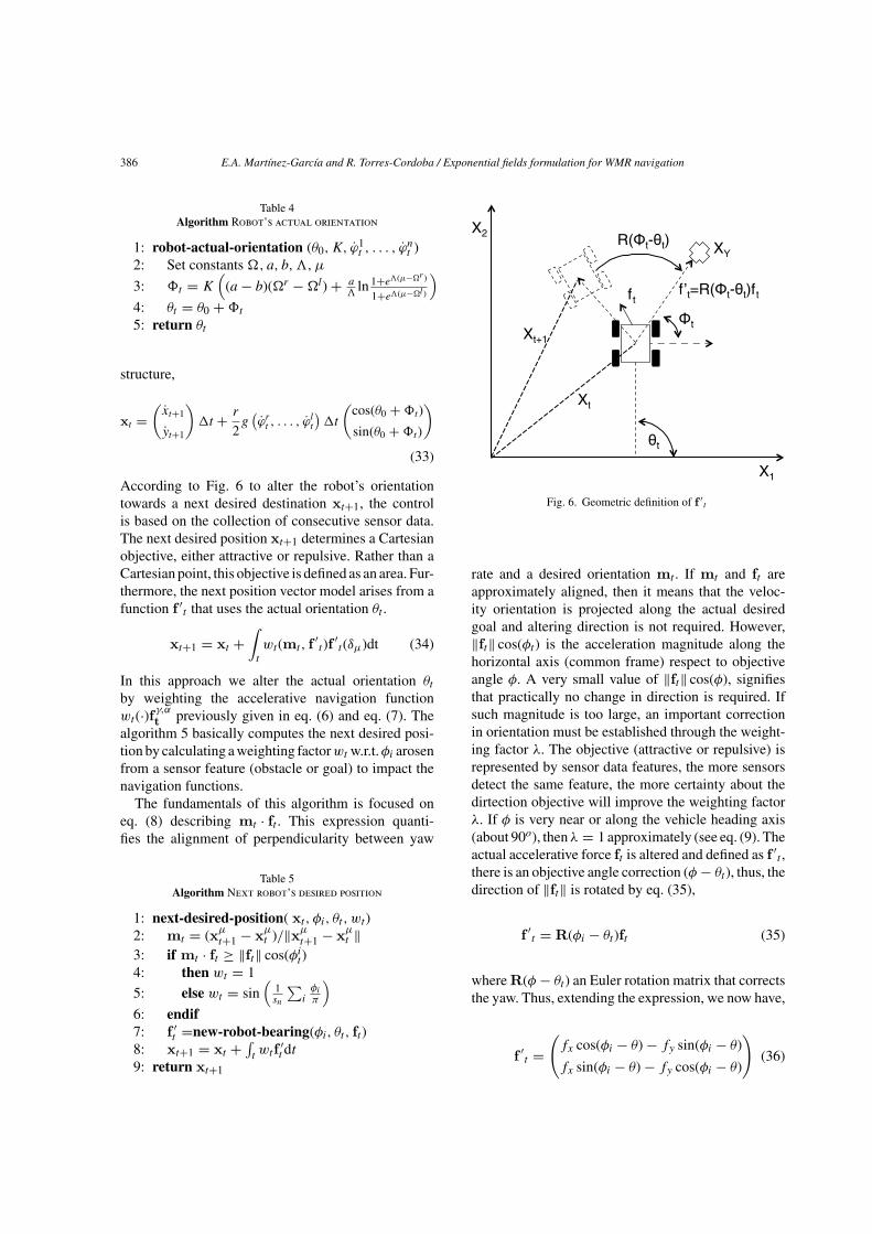
According to Fig. 6 to alter the robot’s orientationtowards a next desired destination xt+1, the controlis based on the collection of consecutive sensor data.The next desired position xt+1 determines a Cartesianobjective, either attractive or repulsive. Rather than aCartesian point, this objective is defined as an area. Fur-thermore, the next position vector model arises from afunction f ′

t that uses the actual orientation θt .

xt+1 = xt +∫t

wt(mt , f ′t)f ′

t(δµ)dt (34)

In this approach we alter the actual orientation θtby weighting the accelerative navigation functionwt(·)fγ,αt previously given in eq. (6) and eq. (7). Thealgorithm 5 basically computes the next desired posi-tion by calculating a weighting factorwt w.r.t.φi arosenfrom a sensor feature (obstacle or goal) to impact thenavigation functions.

The fundamentals of this algorithm is focused oneq. (8) describing mt · ft . This expression quanti-fies the alignment of perpendicularity between yaw

Table 5Algorithm Next robot’s desired position

1: next-desired-position( xt , φi, θt, wt)2: mt = (xµt+1 − xµt )/‖xµt+1 − xµt ‖3: if mt · ft ≥ ‖ft‖ cos(φit)4: then wt = 1

5: else wt = sin(

1sn

∑iφiπ

)6: endif7: f ′

t =new-robot-bearing(φi, θt, ft)8: xt+1 = xt +

∫twtf ′

t dt9: return xt+1

Fig. 6. Geometric definition of f ′t

rate and a desired orientation mt . If mt and ft areapproximately aligned, then it means that the veloc-ity orientation is projected along the actual desiredgoal and altering direction is not required. However,‖ft‖ cos(φt) is the acceleration magnitude along thehorizontal axis (common frame) respect to objectiveangle φ. A very small value of ‖ft‖ cos(φ), signifiesthat practically no change in direction is required. Ifsuch magnitude is too large, an important correctionin orientation must be established through the weight-ing factor λ. The objective (attractive or repulsive) isrepresented by sensor data features, the more sensorsdetect the same feature, the more certainty about thedirtection objective will improve the weighting factorλ. If φ is very near or along the vehicle heading axis(about 90o), thenλ = 1 approximately (see eq. (9). Theactual accelerative force ft is altered and defined as f ′

t ,there is an objective angle correction (φ − θt), thus, thedirection of ‖ft‖ is rotated by eq. (35),

f ′t = R(φi − θt)ft (35)

where R(φ − θt) an Euler rotation matrix that correctsthe yaw. Thus, extending the expression, we now have,

f ′t =

(fx cos(φi − θ) − fy sin(φi − θ)

fx sin(φi − θ) − fy cos(φi − θ)

)(36)


by developing in the vector form f ′t = (fx, fy)T , the

new next-position vector,

xt+1 =(xt

yt

)+∫∫

t

f ′t d2t =

(xt

yt

)

+∫∫

t

(fx cos(φ − θt) − fy sin(φ − θt)

fx sin(φ − θt) − fy cos(φ − θt)

)d2t

(37)

The new desired direction w.r.t. the actual orientationis given by the vector f ′

t , which is a transformationinto the global coordinate frame, since observationsare locals. See Table 6,

Table 6Algorithm New robot’s desired bearing

1: new-robot-bearing(φi, θt, ft)2: f ′

t = R(φi − θt)ft3: return f ′

8. Navigation using directional fields

A gradient vector field assigns the gradient of somefunction to each Cartesian point. The potential func-tion approach directs a robot as if it were moving ina gradient vector field. Gradients can be viewed asaccelerations acting on a positive sense, attracted tothe negative goal. Obstacles also have a positive sensewhich forms a repulsive acceleration directing therobot away from obstacles. The combination of repul-sive and attractive accelerations directs the robot fromthe start location to the goal location while avoidingobstacles. Thus, a potential function is a differentiablereal-valued function, which can be viewed as energy,and hence the gradient of the potential is acceleration.The gradient is a vector which points in the directionthat locally maximises the function.

8.1. Repulsive function

Repulsive potential fields are suitable navigationfunctions that define the path course of a robot to safelyavoid collisions. There exist an important number ofpotential functions that describe numerous behavioursChoset et al. [39]. The actual research work followsthe approach of the social force model, which is basedon exponential distributions. For the case of obsta-cles avoidance, eq. (38) is a general exponential-basedpotential field function. fαt is a scalar that exhibits a

Table 7Algorithm Repulsive accelerative force

1: repulsive-acceleration( uoα, R,xt)2: XI

t = read-from-lidar(θt,xt)3: for j=1 to num-obstacles(XI

t )4: �δt = xα − xt

5: dvαtdt = uoα

‖ �δi‖e‖ �δi‖/R

(1

‖ �δi‖ − R�δi

)(xα − xµ, yα − yµ)T

6: Fαt = Fαt + dvαtdt

7: endfor8: return Fαt

general 1D repulsive potential behaviour (Fig. 7 right).uoα is a constant that adjusts the acceleration amplitude.R is a stationary value defining the territorial objectregion, or defined as the asymptotic potential fallingvalue.

fαt = −∇µαuoαRe‖xα−xµ‖/R

‖xα − xµ‖ (38)

The denominator is determined by the factor(R−1‖xα − xµ‖) and defines the function to respondfast against situations in too close interaction withobstacles. Solving for its gradient operator, we obtain

that fαt ≡(∂f∂x, ∂f∂x

)(see Appendix B).

fαt = uoαe‖�δµα‖/R

‖�δµα‖(

1

‖�δµα‖− R

�δµα)

(xα − xµ

yα − yµ

)(39)

Previous expression is defined in terms of velocities by(40), where such term will satisfy the real velocity ofequation (22),

vαt =∫t

fαt dt (40)

The repulsive directional fields feedback by sensorobservations are computed by the algorithm 7. In thismanuscript we calculate artificial repulsive fields usingonly LIDAR data, because of the ranged nature of data,which makes easier and accurate the social fields map.

8.2. Attractive function

Similarly, equations controlling the robot course toa global goal destination yield motion behaviour asdepicted by Fig. 7-left. A goal destination γ is not


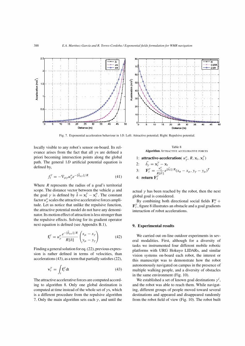
Fig. 7. Exponential acceleration behaviour in 1D. Left: Attractive potential; Right: Repulsive potential.

locally visible to any robot’s sensor on-board. Its rel-evance arises from the fact that all γs are defined apriori becoming intersection points along the globalpath. The general 1D artificial potential equation isdefined by,

fγt = −∇µγuoγe−‖�δµγ‖/R (41)

Where R represents the radius of a goal’s territorialscope. The distance vector between the vehicle µ andthe goal γ is defined by �δ = xγt − xµt . The constantfactoruoγ scales the attractive accelerative forces ampli-tude. Let us notice that unlike the repulsive function,the attractive potential model do not have any denomi-nator. Its motion effect of attraction is less stronger thanthe repulsive effects. Solving for its gradient operatornext equation is defined (see Appendix B.1),

fγt = uoγe−‖�δµγ‖/R

R‖δ‖

(xµ − xγ

yµ − yγ

)(42)

Finding a general solution for eq. (22), previous expres-sion is rather defined in terms of velocities, thanaccelerations (43), as a term that partially satisfies (22),

vγt =∫t

fγt dt (43)

The attractive accelerative forces are computed accord-ing to algorithm 8. Only one global destination iscomputed at time instead of the whole set of γs, whichis a different procedure from the repulsive algorithm7. Only the main algorithm sets each γ , and until the

Table 8Algorithm Attractive accelerative forces

1: attractive-acceleration( uoγ, R,xt ,xγt )

2: �δγ = xγt − xt3: Fγt = uoγ

R‖ �δi‖e‖ �δi‖/R(xα − xµ, yγ − yµ)T

4: return Fγt

actual γ has been reached by the robot, then the nextglobal goal is considered.

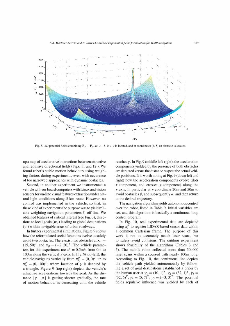
By combining both directional social fields Fαt +Fγt , figure 8 illustrates an obstacle and a goal gradientsinteraction of robot accelerations.

9. Experimental results

We carried out on-line outdoor experiments in sev-eral modalities. First, although for a diversity oftasks we instrumented four different mobile roboticplatforms with URG Hokuyo LIDARs, and similarvision systems on-board each robot, the interest orthis manuscript was to demonstrate how the robotautonomously navigated on campus in the presence ofmultiple walking people, and a diversity of obstaclesin the same environment (Fig. 10).

We established a set of known goal destinations γi,and the robot was able to reach them. While navigat-ing, different groups of people moved toward severaldestinations and appeared and disappeared randomlyfrom the robot field of view (Fig. 10). The robot built


Fig. 8. 3D potential fields combining Fγ + Fα, at < −5, 0 > γ is located, and at coordinates (4, 5) an obstacle is located.

up a map of accelerative interactions between attractiveand repulsive directional fields (Figs. 11 and 12 ). Wefound robot’s stable motion behaviours using weigh-ing factors during experiments, even with occurenceof too narrowed approaches with dynamic obstacles.

Second, in another experiment we instrumented avehicle with on-board computers with Linux and visionsensors for on-line visual features extraction under nat-ural light conditions along 5 km route. However, nocontrol was implemented in the vehicle, so that, inthese kind of experiments the purpose was to yield reli-able weighting navigation parameters δt off-line. Weobtained features of critical interest (see Fig. 3), direc-tions to local goals (mt) leading to global destinations(γi) within navigable areas of urban roadways.

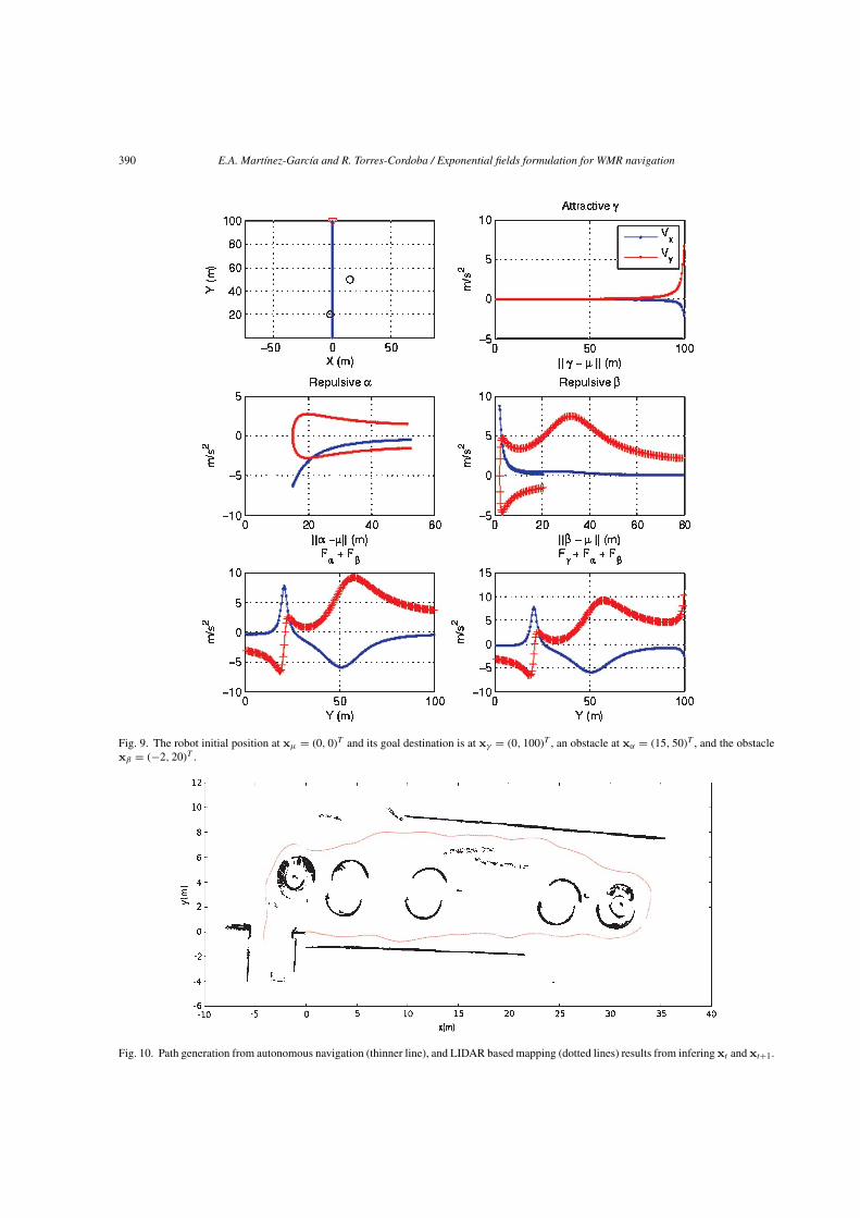
In further experimental simulations, Figure 9 showshow the reformulated social functions evolve to safelyavoid two obstacles. There exist two obstacles at xα =(15, 50)T and xβ = (−2, 20)T . The vehicle parame-ters for this experiment are vo = 0.5m/s from 0m to100m along the vertical Y -axis. In Fig. 9(top-left), thevehicle navigates vertically from xµt0 = (0, 0)T up toxµtn = (0, 100)T , where location of γ is denoted bya triangle. Figure 9 (top-right) depicts the vehicle’sattractive accelerations towards the goal. As the dis-tance ‖γ − µ‖ is getting shorter gradually, the rateof motion behaviour is decreasing until the vehicle

reaches γ . In Fig. 9 (middle left-right), the accelerationcomponents yielded by the presence of both obstaclesare depicted versus the distance respect the actual vehi-cle positions. It is worth noting at Fig. 9 (down left andright) how the acceleration components evolve (dotsx-component, and crosses y-component) along they-axis. In particular at y-coordinate 20m and 50m toavoid obstacles β, and subsequently α, and then returnto the desired trajectory.

The navigation algorithm yields autonomous controlover the robot, listed in Table 9. Initial variables areset, and this algorithm is basically a continuous loopcontrol program.

In Fig. 10, real experimental data are depictedusing xµt to register LIDAR-based sensor data withina common Cartesian frame. The purpose of thiswork is not to accurately match laser scans, butto safely avoid collisions. The outdoor experimentshows feasibility of the algorithms (Tables 3 and5). The mobile robot collected more than 50, 000laser scans within a coursed path nearly 100m long.According to Fig. 10, the continuous line depictsthe vehicle path yielded autonomously by follow-ing a set of goal destinations established a priori bythe human user at γ1 = (10, 1)T , γ2 = (32, 1)T , γ3 =(32, 6)T , γ4 = (5, 7)T , γ5 = (−3, 3)T . The potentialfields repulsive influence was yielded by each of


Fig. 9. The robot initial position at xµ = (0, 0)T and its goal destination is at xγ = (0, 100)T , an obstacle at xα = (15, 50)T , and the obstaclexβ = (−2, 20)T .

Fig. 10. Path generation from autonomous navigation (thinner line), and LIDAR based mapping (dotted lines) results from infering xt and xt+1.


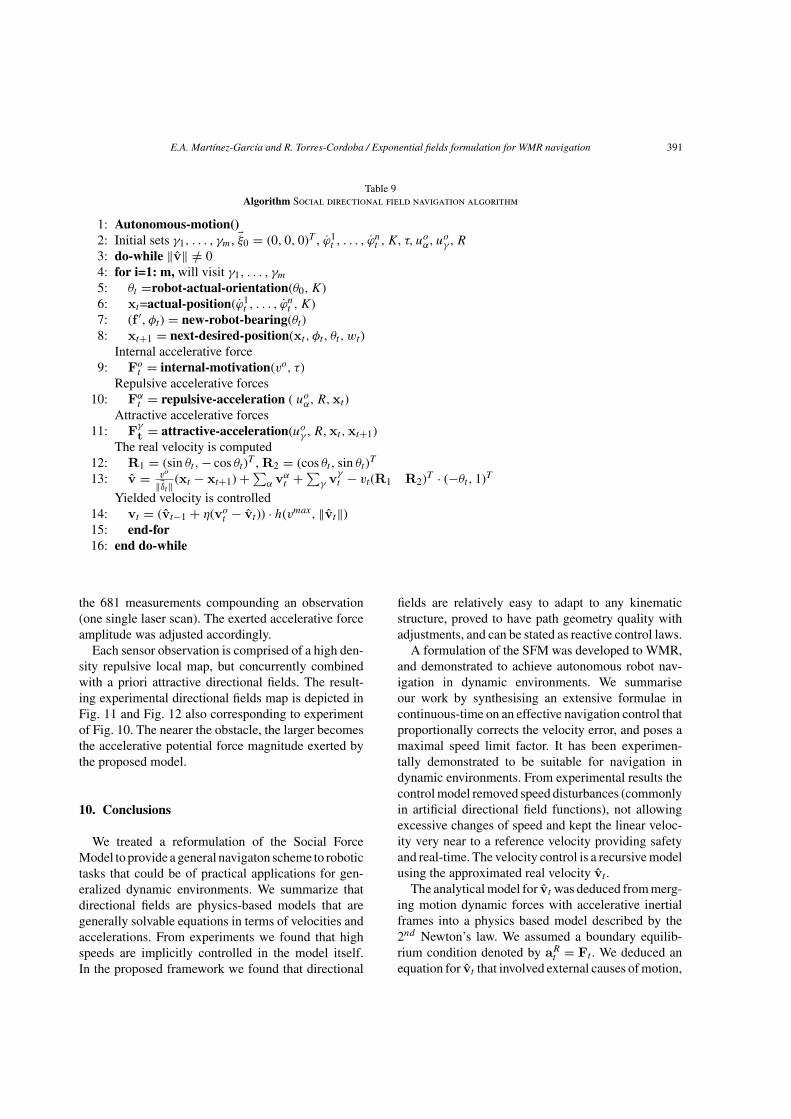
Table 9Algorithm Social directional field navigation algorithm

1: Autonomous-motion()2: Initial sets γ1, . . . , γm, �ξ0 = (0, 0, 0)T , ϕ1

t , . . . , ϕnt , K, τ, u

oα, u

oγ , R

3: do-while ‖v‖ /= 04: for i=1: m, will visit γ1, . . . , γm5: θt =robot-actual-orientation(θ0,K)6: xt=actual-position(ϕ1

t , . . . , ϕnt , K)

7: (f ′, φt) = new-robot-bearing(θt)8: xt+1 = next-desired-position(xt , φt, θt, wt)

Internal accelerative force9: Fot = internal-motivation(vo, τ)

Repulsive accelerative forces10: Fαt = repulsive-acceleration ( uoα, R,xt)

Attractive accelerative forces11: Fγt = attractive-acceleration(uoγ, R,xt ,xt+1)

The real velocity is computed12: R1 = (sin θt,− cos θt)T , R2 = (cos θt, sin θt)T

13: v = vo

‖�δt‖ (xt − xt+1) +∑α vαt +∑γ vγt − vt(R1 R2)T · (−θt, 1)T

Yielded velocity is controlled14: vt = (vt−1 + η(vot − vt)) · h(vmax, ‖vt‖)15: end-for16: end do-while

the 681 measurements compounding an observation(one single laser scan). The exerted accelerative forceamplitude was adjusted accordingly.

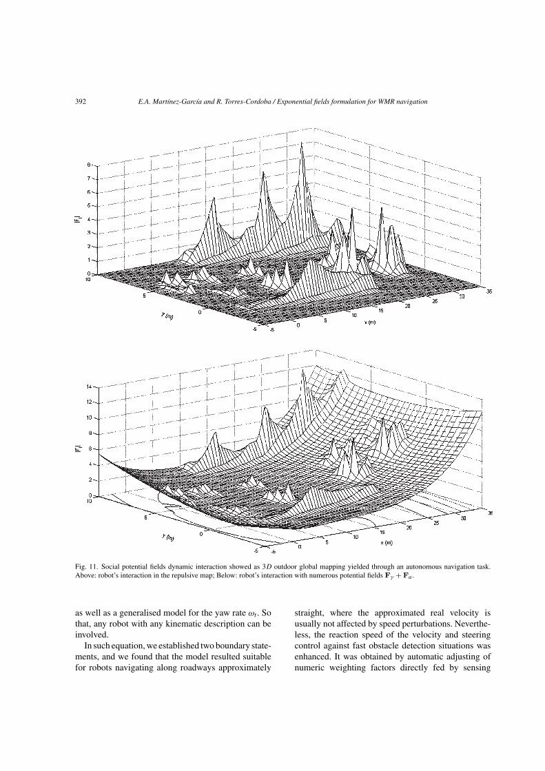
Each sensor observation is comprised of a high den-sity repulsive local map, but concurrently combinedwith a priori attractive directional fields. The result-ing experimental directional fields map is depicted inFig. 11 and Fig. 12 also corresponding to experimentof Fig. 10. The nearer the obstacle, the larger becomesthe accelerative potential force magnitude exerted bythe proposed model.

10. Conclusions

We treated a reformulation of the Social ForceModel to provide a general navigaton scheme to robotictasks that could be of practical applications for gen-eralized dynamic environments. We summarize thatdirectional fields are physics-based models that aregenerally solvable equations in terms of velocities andaccelerations. From experiments we found that highspeeds are implicitly controlled in the model itself.In the proposed framework we found that directional

fields are relatively easy to adapt to any kinematicstructure, proved to have path geometry quality withadjustments, and can be stated as reactive control laws.

A formulation of the SFM was developed to WMR,and demonstrated to achieve autonomous robot nav-igation in dynamic environments. We summariseour work by synthesising an extensive formulae incontinuous-time on an effective navigation control thatproportionally corrects the velocity error, and poses amaximal speed limit factor. It has been experimen-tally demonstrated to be suitable for navigation indynamic environments. From experimental results thecontrol model removed speed disturbances (commonlyin artificial directional field functions), not allowingexcessive changes of speed and kept the linear veloc-ity very near to a reference velocity providing safetyand real-time. The velocity control is a recursive modelusing the approximated real velocity vt .

The analytical model for vt was deduced from merg-ing motion dynamic forces with accelerative inertialframes into a physics based model described by the2nd Newton’s law. We assumed a boundary equilib-rium condition denoted by aRt = Ft . We deduced anequation for vt that involved external causes of motion,


Fig. 11. Social potential fields dynamic interaction showed as 3D outdoor global mapping yielded through an autonomous navigation task.Above: robot’s interaction in the repulsive map; Below: robot’s interaction with numerous potential fields Fγ + Fα.

as well as a generalised model for the yaw rate ωt . Sothat, any robot with any kinematic description can beinvolved.

In such equation, we established two boundary state-ments, and we found that the model resulted suitablefor robots navigating along roadways approximately

straight, where the approximated real velocity isusually not affected by speed perturbations. Neverthe-less, the reaction speed of the velocity and steeringcontrol against fast obstacle detection situations wasenhanced. It was obtained by automatic adjusting ofnumeric weighting factors directly fed by sensing


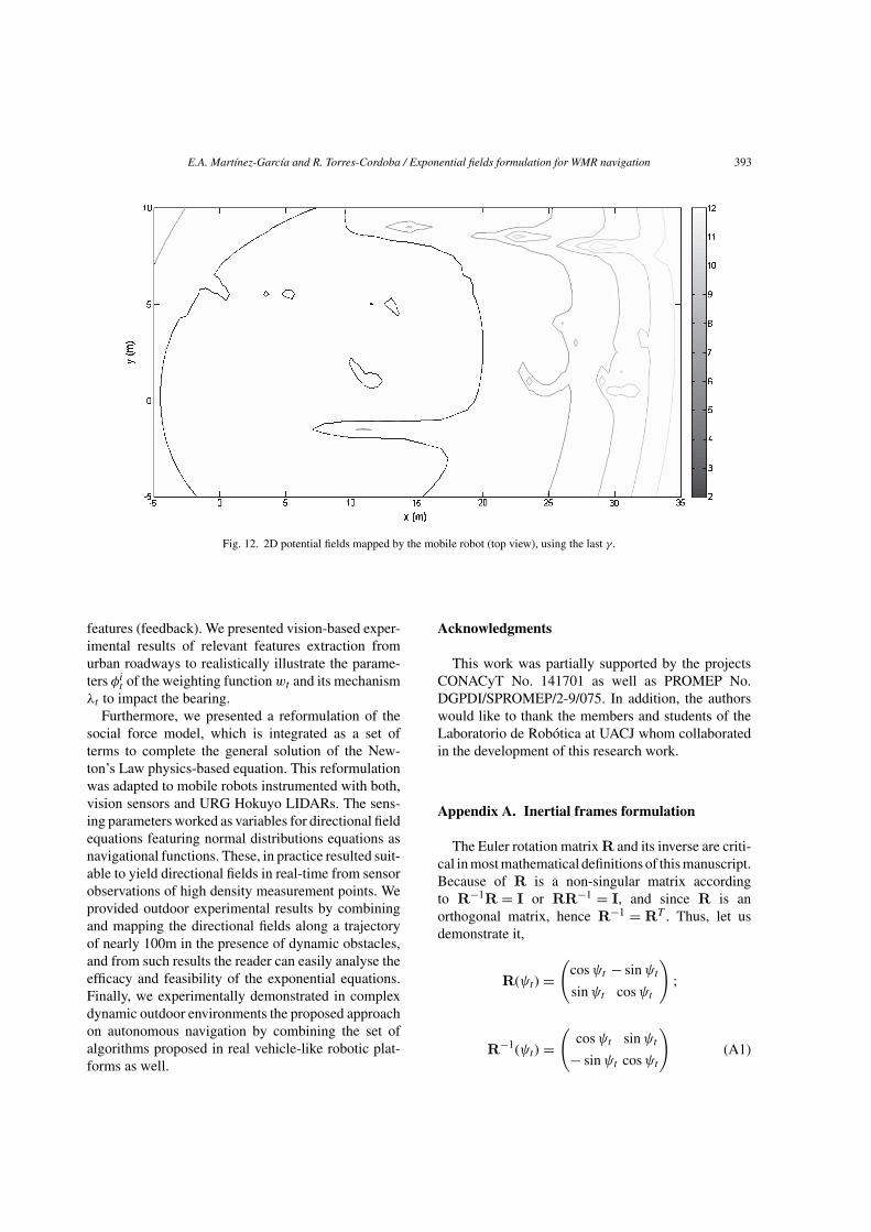
Fig. 12. 2D potential fields mapped by the mobile robot (top view), using the last γ .

features (feedback). We presented vision-based exper-imental results of relevant features extraction fromurban roadways to realistically illustrate the parame-ters φit of the weighting functionwt and its mechanismλt to impact the bearing.

Furthermore, we presented a reformulation of thesocial force model, which is integrated as a set ofterms to complete the general solution of the New-ton’s Law physics-based equation. This reformulationwas adapted to mobile robots instrumented with both,vision sensors and URG Hokuyo LIDARs. The sens-ing parameters worked as variables for directional fieldequations featuring normal distributions equations asnavigational functions. These, in practice resulted suit-able to yield directional fields in real-time from sensorobservations of high density measurement points. Weprovided outdoor experimental results by combiningand mapping the directional fields along a trajectoryof nearly 100m in the presence of dynamic obstacles,and from such results the reader can easily analyse theefficacy and feasibility of the exponential equations.Finally, we experimentally demonstrated in complexdynamic outdoor environments the proposed approachon autonomous navigation by combining the set ofalgorithms proposed in real vehicle-like robotic plat-forms as well.

Acknowledgments

This work was partially supported by the projectsCONACyT No. 141701 as well as PROMEP No.DGPDI/SPROMEP/2-9/075. In addition, the authorswould like to thank the members and students of theLaboratorio de Robotica at UACJ whom collaboratedin the development of this research work.

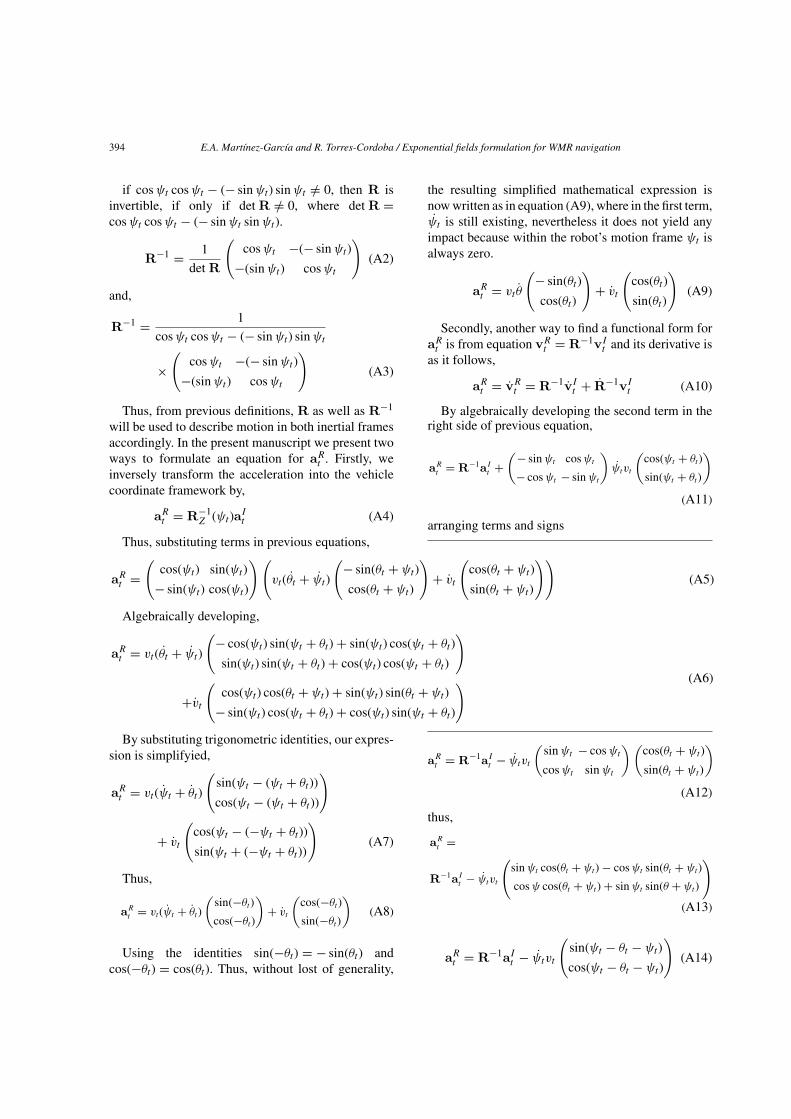
Appendix A. Inertial frames formulation

The Euler rotation matrix R and its inverse are criti-cal in most mathematical definitions of this manuscript.Because of R is a non-singular matrix accordingto R−1R = I or RR−1 = I, and since R is anorthogonal matrix, hence R−1 = RT . Thus, let usdemonstrate it,

R(ψt) =(

cosψt − sinψtsinψt cosψt

);

R−1(ψt) =(

cosψt sinψt− sinψt cosψt

)(A1)


if cosψt cosψt − (− sinψt) sinψt /= 0, then R isinvertible, if only if det R /= 0, where det R =cosψt cosψt − (− sinψt sinψt).

R−1 = 1

det R

(cosψt −(− sinψt)

−(sinψt) cosψt

)(A2)

and,

R−1 = 1

cosψt cosψt − (− sinψt) sinψt

×(

cosψt −(− sinψt)

−(sinψt) cosψt

)(A3)

Thus, from previous definitions, R as well as R−1

will be used to describe motion in both inertial framesaccordingly. In the present manuscript we present twoways to formulate an equation for aRt . Firstly, weinversely transform the acceleration into the vehiclecoordinate framework by,

aRt = R−1Z (ψt)aIt (A4)

Thus, substituting terms in previous equations,

aRt =(

cos(ψt) sin(ψt)

− sin(ψt) cos(ψt)

)(vt(θt + ψt)

(− sin(θt + ψt)

cos(θt + ψt)

)+ vt

(cos(θt + ψt)

sin(θt + ψt)

))(A5)

Algebraically developing,

aRt = vt(θt + ψt)

(− cos(ψt) sin(ψt + θt) + sin(ψt) cos(ψt + θt)

sin(ψt) sin(ψt + θt) + cos(ψt) cos(ψt + θt)

)

+vt(

cos(ψt) cos(θt + ψt) + sin(ψt) sin(θt + ψt)

− sin(ψt) cos(ψt + θt) + cos(ψt) sin(ψt + θt)

) (A6)

By substituting trigonometric identities, our expres-sion is simplifyied,

aRt = vt(ψt + θt)

(sin(ψt − (ψt + θt))

cos(ψt − (ψt + θt))

)

+ vt

(cos(ψt − (−ψt + θt))

sin(ψt + (−ψt + θt))

)(A7)

Thus,

aRt = vt(ψt + θt)

(sin(−θt)cos(−θt)

)+ vt

(cos(−θt)sin(−θt)

)(A8)

Using the identities sin(−θt) = − sin(θt) andcos(−θt) = cos(θt). Thus, without lost of generality,

the resulting simplified mathematical expression isnow written as in equation (A9), where in the first term,ψt is still existing, nevertheless it does not yield anyimpact because within the robot’s motion frame ψt isalways zero.

aRt = vtθ

(− sin(θt)

cos(θt)

)+ vt

(cos(θt)

sin(θt)

)(A9)

Secondly, another way to find a functional form foraRt is from equation vRt = R−1vIt and its derivative isas it follows,

aRt = vRt = R−1vIt + R−1vIt (A10)

By algebraically developing the second term in theright side of previous equation,

aRt = R−1aIt +(− sinψt cosψt

− cosψt − sinψt

)ψtvt

(cos(ψt + θt)

sin(ψt + θt)

)

(A11)

arranging terms and signs

aRt = R−1aIt − ψtvt

(sinψt − cosψtcosψt sinψt

)(cos(θt + ψt)

sin(θt + ψt)

)

(A12)

thus,

aRt =

R−1aIt − ψtvt

(sinψt cos(θt + ψt) − cosψt sin(θt + ψt)

cosψ cos(θt + ψt) + sinψt sin(θ + ψt)

)

(A13)


(sin(ψt − θt − ψt)

cos(ψt − θt − ψt)

)(A14)


and


(− sin θtcos θt

)(A15)

Now, developing the first term of right-side of equa-tion,

aIt = vt(θt)

(− sin θt

cos θ

)+ vt

(cos θtsin θt

)

− ψt tvt

(− sin θtcos θt

)(A16)

Finally,

aIt = vtθt

(− sin θtcos θt

)+ vt

(cos θt

− sin θt

)(A17)

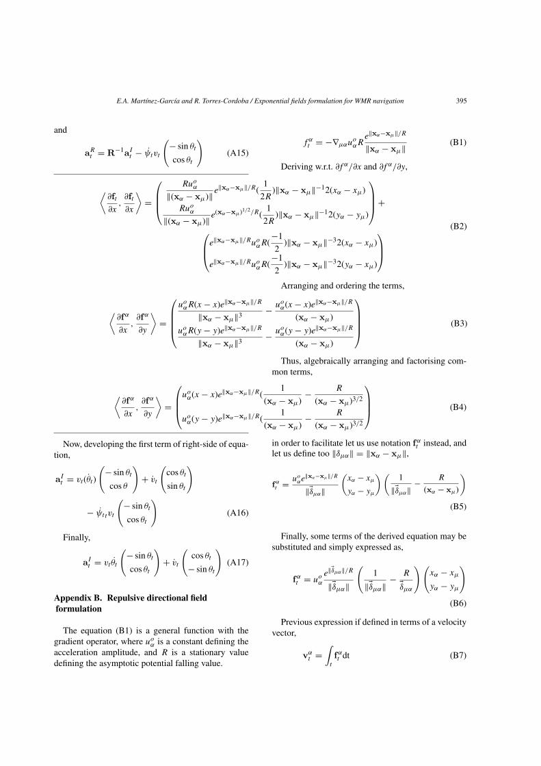
Appendix B. Repulsive directional fieldformulation

The equation (B1) is a general function with thegradient operator, where uoα is a constant defining theacceleration amplitude, and R is a stationary valuedefining the asymptotic potential falling value.

fαt = −∇µαuoαRe‖xα−xµ‖/R

‖xα − xµ‖ (B1)

Deriving w.r.t. ∂fα/∂x and ∂fα/∂y,

⟨∂ft∂x,∂ft∂x

⟩=

⎛⎜⎜⎝

Ruoα

‖(xα − xµ)‖e‖xα−xµ‖/R(

1

2R)‖xα − xµ‖−12(xα − xµ)

Ruoα

‖(xα − xµ)‖e(xα−xµ)1/2/R(

1

2R)‖xα − xµ‖−12(yα − yµ)

⎞⎟⎟⎠+

⎛⎜⎝e

‖xα−xµ‖/RuoαR(−1

2)‖xα − xµ‖−32(xα − xµ)

e‖xα−xµ‖/RuoαR(−1

2)‖xα − xµ‖−32(yα − xµ)

⎞⎟⎠

(B2)

Arranging and ordering the terms,

⟨∂fα

∂x,∂fα

∂y

⟩=

⎛⎜⎜⎜⎝uoαR(x− x)e‖xα−xµ‖/R

‖xα − xµ‖3 − uoα(x− x)e‖xα−xµ‖/R

(xα − xµ)

uoαR(y − y)e‖xα−xµ‖/R

‖xα − xµ‖3 − uoα(y − y)e‖xα−xµ‖/R

(xα − xµ)

⎞⎟⎟⎟⎠ (B3)

Thus, algebraically arranging and factorising com-mon terms,

⟨∂fα

∂x,∂fα

∂y

⟩=

⎛⎜⎜⎝uoα(x− x)e‖xα−xµ‖/R(

1

(xα − xµ)− R

(xα − xµ)3/2

uoα(y − y)e‖xα−xµ‖/R(1

(xα − xµ)− R

(xα − xµ)3/2

⎞⎟⎟⎠ (B4)

in order to facilitate let us use notation fαt instead, andlet us define too ‖δµα‖ = ‖xα − xµ‖,

fαt = uoαe‖xα−xµ‖/R

‖�δµα‖

(xα − xµ

yα − yµ

)(1


(xα − xµ)

)

(B5)

Finally, some terms of the derived equation may besubstituted and simply expressed as,

fαt = uoαe‖�δµα‖/R

‖�δµα‖

(1


�δµα

)(xα − xµ

yα − yµ

)

(B6)

Previous expression if defined in terms of a velocityvector,

vαt =∫t

fαt dt (B7)


B.1. Attractive directional field formulation

The attractive potential function general equation isdefined by,

fγt = −∇µγuoe−‖�δµγ‖/R (B8)

Thus, by deriving the function w.r.t.x andy, it yields,

⟨∂fγt∂x,∂fγt∂y

⟩=

⎛⎜⎝−uoe−‖xγ−xµ‖/R(

−1

2)‖xγ − xµ‖

R2(xγ − xµ)

−uoe−‖xγ−xµ‖/R(−1

2)‖xγ − xµ‖

R2(yγ − yµ)

⎞⎟⎠ (B9)

simplifying the expression it now becomes

fγt = uoe−‖xγ−xµ‖/R⎛⎝ xγ−xµR‖xγ−xµ‖yγ−yµ

R‖xγ−xµ‖

⎞⎠ (B10)

Algebraically arranging, the 2D potential functionbecomes as follows,

fγt = uoe−‖�δµγ‖/R

R‖�δ‖

(xµ − xγ

yµ − yγ

)(B11)

References

[1] W.H. Huang, B.R. Fajen, J.R. Fink and W.H. Warren, Visualnavigation and obstacle avoidance using a steering potentialfunction, Robotics and Autonomous Systems 54 (2005), pp.288–299, ISSN 0921-8890.

[2] M.F. Selekwa, D.D. Dunlap, D. Shi and E.G. Collins Jr., Robotnavigation in very cluttered environments by preference-based fuzzy behaviors, Robotics and Autonomous Systems56 (2007), pp. 231–246.

[3] M.C. Mora and J. Tornero, Path planning and trajectory gen-eration using multi-rate predictive artificial potential fields,IEEE/RSJ International Conference on Intelligent Robotsand Systems, Acropolis Convention Center, Nice France, pp.2990–2995, 2008, ISBN 978-1-4244-2058-2.

[4] A.A. Masound, Managing the dynamics of a harmonic poten-tial field-guided robot in a cluttered environment, IEEETransaction on Industrial Electronics 56(2), February 2010,pp. 488–496.

[5] V.M. Goncalves, L.C.A. Pimienta, C.A. Maia, B.C.O. Dutraand G.A.A. Pereira, Vector fields for robot navigation alongtime-varying curves in n-dimensions, IEEE Transactions onRobotics 26(4) August 2010, pp. 647–659, ISSN 1552-3098.

[6] M. Werling, L. Groll and G. Bretthauer, Invariant trajec-tory tracking with a full-size autonomous road vehicle, IEEETransactions on Robotics 26(4), August 2010, pp. 758–765,ISSN 1552-3098.

[7] L.A. Tychonievich, R.P. Burton and L.P. Tychonievich, Versa-tile Reactive Navigation, IEEE/RSJ International Conferenceon Intelligent Robots and Systems, Octover 11–15, USA, pp.2966–2972, 2009, ISBN 978-1-4244-3804-4.

[8] A. Broggi, L. Bombini, S. Cattani, P. Cerri and R.I. Fedriga,Sensing requirements for a 13, 000 km intercontinentalAutonomous drive, IEEE Intelligent Vehicles Symposium,San Diego California, USA, June 21–24, pp. 500–505, 2010,ISBN 978-1-4244-7868-2.

[9] G. Stanek, D. Langer and M. Muller-Bessler, JUNIOR 3:Test platform for advanced driver assistance systems, IEEEIntelligent Vehicles Symposium, Unoversity of California SanDiego, June 21–24, pp. 143–149, 2010, ISB 978-1-4244-7868-2.

[10] A. Teja, d. Karthikeya and K. Madhava A mixed autonomycoordination methodology for multi-robotic traffic control,IEEE International Conference on Robotics and Biomimetics,Bankok, Thailand, pp. 1273–1278, 2009, ISBN 978-1-4244-2679–9.

[11] E. Plaku, L.E. Kavraki and M. Vardi, Motion planningwith dynamics by synergistic combination of layers of plan-ning, IEEE Transaction on Robotics 26(3) (2010), pp. 469–482.

[12] K. Moriwaki and K. Tanaka, Navigation control for electricvehicles using nonlinear state feedback H∞ control, Nonlin-ear Analysis 71 (2009), pp. e2020–e2933.

[13] K. Iagnemma, S. Shimoda and Z. Shiller, Near-optimalnavigation of high speed mobile robots on uneven terrain,IEEE/RSJ Intl. Conference on Intelligent Robots and Sys-tems, Acropolis Convention Center, Nice France, Sept. 22–26,2008, pp. 4098–4013, ISBN 978-1-42442058-2/08.

[14] M.P. Mann and Z. Shiller, “Dynamic stability of off-road vehi-cles: A geometric approach,” Proceedings of IEEE Int. Conf.on Robotics and Automation 2006, pp. 3705–3710.

[15] S. Geand and Y. Cui, Dynamic motion planning for mobilerobots using potential field method, Autonomous Robots 13(2002).

[16] D. Helbing and P. Molnar, “Social force model for pedestriansdynamics”, Physical Review E 51 (1995), p. 4282.

[17] S. Shimoda, Y. Kuroda and K. Iagnemma, Potential Field Nav-igation of High Speed unmanned ground vehicles on uneventerrain, Proceedings of the IEEE International Conference onRobotics and Automation, Barcelona, Spain, April 2005.

[18] Kareem Mohammad, Garibeh Mohammad and Feilat Eyad,Dynamic motion planning for autonomous mobile robot usingfuzzy potential field, Proceeding of the 6th International Sym-posium on Mechatronics and its applications, Sharjah, UAE,March 24–26, 2009.

[19] Dimitar Baronov and John Baillieul, Autonomous vehiclecontrol for ascending/descending along a potential field withtwo applications, 2008 American Control Conference, WestinSeattle Hotel, Seattle, Washington, USA, June 11–13, 2008,p. 678–683.

[20] Jing Ren, Kenneth A. McIsaac, Rajni V. Patel and TerryM. Peters, A Potential Field Model Using Generalized Sig-moid Functions, IEEE Transactions on Systems, Man andCybernetics-Part B: Cybernetics 37(2), April 2007, pp.447–484.

[21] Jiangmin Chunyu, Zhihua Qu, Eytan Pollak and Mark Falash,A new reactive target-tracking control with obstacle avoid-ance in a dynamic environment, 2009 American Control


Conference, Hyatt Regency Riverfront, St. Louis, MO, USA,June 10–12, 2009, pp. 3872–3877.

[22] S.H.I. Enxiu, C.A.I. Tao, H.E. Changlin, S.H.I. Enxiu andG.U.O. Junjie, Study of the New Method for ImprovingArtificial Potential Field in Mobile Robot Obstacle Avoid-ance, Proceedings of the IEEE International Conference onAutomation and Logistics, August 18–21, Jinan, China, 2007,p. 282–286.

[23] Samer Charifa and Marwan Bikdash, Comparison of geo-metrical, kinematic, and dynamic performance of severalpotential field methods, IEEE Southeastcon 2009, March 5–8,2009, pp. 18–23.

[24] Richard Bishop, A survey of intelligent vehicle applicationsworldwide, Proceedings of the IEEE intelligent Vehicles Sym-posium 2000, Dearborn (MI), USA, October 3–5, 2000, pp.25–30.

[25] Yang Chen, Hangen He, and Xiangjing An, Motion planningof intelligent vehicles: A survey, IEEE International Confer-ence on Vehicular Electronics and Safety, 2006. ICVES 2006.Dec. 13–15 p. 333–336.

[26] Edgar Martınez-Garcıa, Alfredo Mar, and Rafael Torres-Cordoba, Dead-reckoning inverse and direct kinematicsolution of a 4W independent driven rover, IEEE ANDESCON2010, Bogota Col., Sep 15th–17th, 2010, paper 57, ISBN:978-1-4244-6741-9.

[27] Edgar Martınez-Garcıa and Rafael Torres-Cordoba, 4WDSkid-steer trajectory control of a rover with spring-basedsuspension analysis: Direct and inverse kinematic parame-ters solution, Intelligent Robotics and Applications, SpringerLecture Notes in Computer Science, 6425, Nov. 2010, ISBN978-3-642-16586-2.

[28] G. Campion, G. Baston and B.D. Andrea-Novel, Structuralproperties and classification of kinematic and dynamic mod-els of wheeled mobile robots, IEEE Transaction on Roboticsand Automation 12(1) February 1996.

[29] D. Fox, W. Burgard and S. Thrun, The dynamic windowapproach to collision avoidance, IEEE Robotics & Automa-tion Magazine 4 (1997), pp. 23–33.

[30] S.G. Loizou and K.J. Kyriakopolous, Navigation of multi-ple kinematically constrained robots, IEEE Transactions onRobotics 24(1), February 2008, pp. 221–231.

[31] D. Wang and C.B. Low, Modeling and analysis of skiddingand slipping wheeled mobile robots: Control design perspec-tive, IEEE Transactions on Robotics 24(3) June 2008, pp.676–687.

[32] K. Song and C.C. Chang, Reactive navigation in dynamicenvironment using multisensory predictor, IEEE Transactionson Systems, Man and Cybernetics-Part B: Cybernetics 29(6),December 1999, pp. 870–880.

[33] K. Macek, K. Thoma, R. Glatzel and R. Siewart, Dynam-ics modeling and parameter identification for autonomousvehicle navigation, In Proceedings of the 2007 IEEE/RSJInternational Conference on Intelligent Robots and Systems,2007, pp. 3321–3326.

[34] R. Gayle, W. Moss, M.C. Lin and D. Manocha, Multi-robotcoordination using generalized potential fields, IEEE Interna-tional Conference on Robotics and Automation (ICRA), 2009,pp. 1–8.

[35] R. Benenson, S. Petti, T. Fraichard and M. Parent, Integratingperception and planning for autonomous navigation of urbanvehicles, Proc. of the 2006 IEEE/RSJ International Confer-ence on Intelligent Robots and Systems, October 9–15, 2006,Beijing, China, pp. 98–104.

[36] W. Rong-ben, Z. Rong-hui, J. Li-sheng, G. Xiu-hong andG. Lie, Research on System design and control technologyof vision-based cybercar, Proc. 2006 IEEE/RSJ InternationalConference on Intelligent Robots and systems, October 9–15,Beijing, China.

[37] J.M. Armingol, A. de la Escalera, C. Hilario, J.M. Collado, J.P.Carrasco, M.J. Flores, J.M. Pastor and F.J. Rodriguez, IVVI:Intelligent vehicle based on visual information, Robotics andAutonomous Systems, Science Direct 55, 904–916.

[38] G.E. Brown and A.D. Jackson, The Nucleon-Nucleon Inter-action, North-Holland Publishing, Amsterdam, 1976.

[39] H. Choset, K.M. Lynch, S. Hutchinson, G. Kantor, W. Bur-gard, L.E. Kavraki and S. Thrun, Principles of Robot Motion,Theory, Algorithms and Implementations, MIT Press, 2005.

International Journal of

AerospaceEngineeringHindawi Publishing Corporationhttp://www.hindawi.com Volume 2010

RoboticsJournal of

Hindawi Publishing Corporationhttp://www.hindawi.com Volume 2014


Active and Passive Electronic Components

Control Scienceand Engineering

Journal of



RotatingMachinery


Hindawi Publishing Corporation http://www.hindawi.com

Journal ofEngineeringVolume 2014

Submit your manuscripts athttp://www.hindawi.com

VLSI Design



Shock and Vibration


Civil EngineeringAdvances in

Acoustics and VibrationAdvances in



Electrical and Computer Engineering

Journal of

Advances inOptoElectronics

Hindawi Publishing Corporation http://www.hindawi.com

Volume 2014

The Scientific World JournalHindawi Publishing Corporation http://www.hindawi.com Volume 2014

SensorsJournal of


Modelling & Simulation in EngineeringHindawi Publishing Corporation http://www.hindawi.com Volume 2014


Chemical EngineeringInternational Journal of Antennas and

Propagation




Navigation and Observation



DistributedSensor Networks


Exponential ﬁelds formulation for WMR...

Documents

Transcript of Exponential ﬁelds formulation for WMR...