1

Exploring the Impacts of Large Woody Debris to the Geomorphology of Redwood Creek in Marin County, CA

Investigators

Damon Burgett, Kota Funayama, Allison Hughes

Introduction

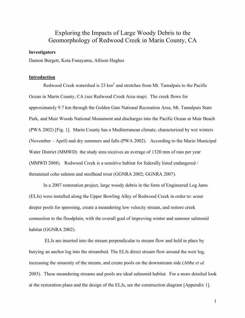
Redwood Creek watershed is 23 km2 and stretches from Mt. Tamalpais to the Pacific

Ocean in Marin County, CA (see Redwood Creek Area map). The creek flows for

approximately 9.7 km through the Golden Gate National Recreation Area, Mt. Tamalpais State

Park, and Muir Woods National Monument and discharges into the Pacific Ocean at Muir Beach

(PWA 2002) [Fig. 1]. Marin County has a Mediterranean climate, characterized by wet winters

(November – April) and dry summers and falls (PWA 2002). According to the Marin Municipal

Water District (MMWD) the study area receives an average of 1320 mm of rain per year

(MMWD 2008). Redwood Creek is a sensitive habitat for federally listed endangered /

threatened coho salmon and steelhead trout (GGNRA 2002; GGNRA 2007).

In a 2007 restoration project, large woody debris in the form of Engineered Log Jams

(ELJs) were installed along the Upper Bowling Alley of Redwood Creek in order to: scour

deeper pools for spawning, create a meandering low velocity stream, and restore creek

connection to the floodplain, with the overall goal of improving winter and summer salmonid

habitat (GGNRA 2002).

ELJs are inserted into the stream perpendicular to stream flow and held in place by

burying an anchor log into the streambed. The ELJs direct stream flow around the weir log,

increasing the sinuosity of the stream, and create pools on the downstream side (Abbe et al.

2003). These meandering streams and pools are ideal salmonid habitat. For a more detailed look

at the restoration plans and the design of the ELJs, see the construction diagram [Appendix 1].

2

Figure 1: Redwood Creek Location and Watershed Boundary (NPS)

Stakeholders

Due to the multiple land-uses that the creek winds through, there are a number of

stakeholders interested in this restoration project: the Golden Gate National Recreation Area

(GGNRA), a division of the National Park Service (NPS); Mt. Tamalpais State Park, a part of the

California Department of Parks and Recreation; Marin Municipal Water District; and the

Residents of Muir Beach. In order to conduct fieldwork in the GGNRA, we obtained a scientific

research and collecting permit through the NPS. This project was conducted under the guidance

of Carolyn Shoulders, Natural Resource Specialist for the GGNRA, and we are very grateful for

her assistance in creating a study design that can be replicated for future geomorphic assessments

of Redwood Creek.

3

Purpose of Study

The purpose of this study was to investigate the impacts of installed large woody debris,

in the form of Engineered Log Jams (ELJs), on the geomorphology of Redwood Creek. The

National Park Service (NPS), the National Oceanic and Atmospheric Administration (NOAA),

National Marine Fisheries Service (NMFS) and the U.S. Fish and Wildlife Service (USFWS)

installed the ELJs in 2003, in the Lower Alley, and in 2007, in the Upper Alley, as part of the

Redwood Creek Salmonid Habitat Restoration Project that is in progress.

The goals of the restoration project are to:

• “Enhance summer rearing and winter refugia habitat for coho and steelhead • Restore stream channel, riparian and floodplain connectivity and ecosystem processes • Enhance nesting habitat for resident and migrant riparian songbirds by widening the riparian

corridor and other feasible methods • Create self-sustaining restored conditions that minimize intervention, management and

maintenance requirements during restoration and into the future, and • Create sustainable breeding habitat for California red-legged frog at the Banducci site in an

effort to expand the local breeding area” (KHE 2007).

Geomorphic assessments conducted at a reach scale are necessary for recognizing the

specific processes that are occurring in the stream (Kondolf & Micheli 1995). Conducting long-

term, repeatable measurements is an essential method for detecting changes over time, which is

an assessment criterion for restoration evaluation (Kondolf 1995; Kondolf & Micheli 1995; Flosi

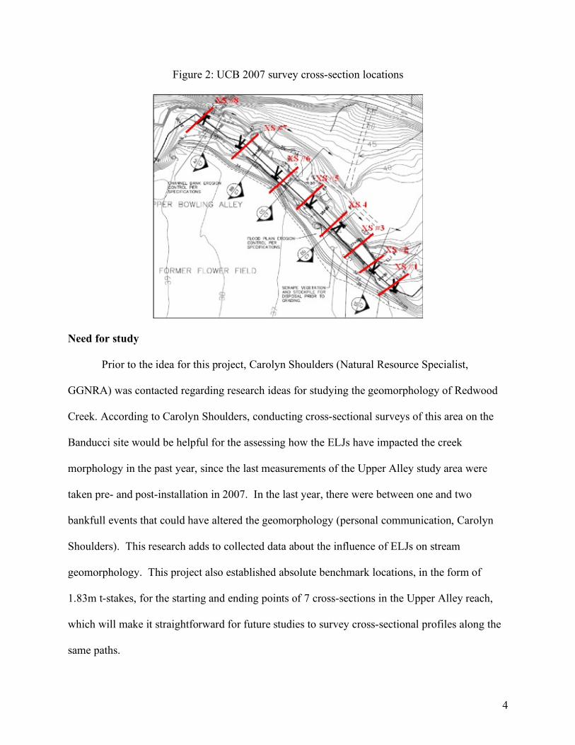
et al. 1998). In 2007, Hsaio Wen, a post-doctoral student from University of California Berkeley

(UCB), performed cross-sectional measurements at the Banducci site. The 2007 UCB study was

used as baseline data for this research project. In accordance with recommended methods

(Kondolf 1995; Flosi et al. 1998), cross-sectional measurements were surveyed along the

approximate past locations [Figure 2].

4

Figure 2: UCB 2007 survey cross-section locations

Need for study

Prior to the idea for this project, Carolyn Shoulders (Natural Resource Specialist,

GGNRA) was contacted regarding research ideas for studying the geomorphology of Redwood

Creek. According to Carolyn Shoulders, conducting cross-sectional surveys of this area on the

Banducci site would be helpful for the assessing how the ELJs have impacted the creek

morphology in the past year, since the last measurements of the Upper Alley study area were

taken pre- and post-installation in 2007. In the last year, there were between one and two

bankfull events that could have altered the geomorphology (personal communication, Carolyn

Shoulders). This research adds to collected data about the influence of ELJs on stream

geomorphology. This project also established absolute benchmark locations, in the form of

1.83m t-stakes, for the starting and ending points of 7 cross-sections in the Upper Alley reach,

which will make it straightforward for future studies to survey cross-sectional profiles along the

same paths.

5

Methods Field research was able to begin after obtaining a Scientific Research and Collecting

Permit from the NPS. Re-occupying cross-section locations was difficult as the UCB 2007 map

included only rough locational estimations, and no absolute coordinates of the starting or ending

points. Field observation showed that the starting and ending points from the UCB 2007 study

were marked on trees using small metal pins. Some of the trees had fallen over and not all of the

cross-sections were able to be re-occupied. In addition to this challenge, the prior cross-section

measurements started and ended around the edge of the bank and did not capture the topography

of the floodplain, or record critical stream conditions such as thalweg locations or bankfull

widths or depths. However, since the 2007 study was the only available data pre-restoration,

every effort possible was made to re-survey approximately the same locations. Cross-section

locations were also interspersed throughout the study site, with some upstream, downstream, and

directly across the ELJs to provide a variety of observations as to how the ELJs are impacting the

channel.

To ensure repeatability, 1.83 meter t-stakes were installed in the floodplain, inline with

past measurements, to define seven cross-section locations [Appendix A1]. Due to time

constraints, only six of the seven established cross-sections were surveyed. Five of the seven

cross-sections that were established this year roughly correlate to the UCB study. One of the

established cross-sections overlays measurements taken by Kamman Hydrology & Engineering,

Inc. (KHE), the engineers who designed and installed the ELJs; this cross-section corresponds to

EE [Figure 2]. Cross-section measurements began on the Westside of the creek and ended on the

Eastside; the terminology used in this report reflects this.

6

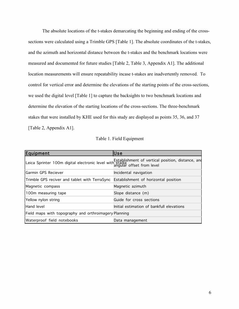
The absolute locations of the t-stakes demarcating the beginning and ending of the cross-

sections were calculated using a Trimble GPS [Table 1]. The absolute coordinates of the t-stakes,

and the azimuth and horizontal distance between the t-stakes and the benchmark locations were

measured and documented for future studies [Table 2, Table 3, Appendix A1]. The additional

location measurements will ensure repeatability incase t-stakes are inadvertently removed. To

control for vertical error and determine the elevations of the starting points of the cross-sections,

we used the digital level [Table 1] to capture the backsights to two benchmark locations and

determine the elevation of the starting locations of the cross-sections. The three-benchmark

stakes that were installed by KHE used for this study are displayed as points 35, 36, and 37

[Table 2, Appendix A1].

Table 1. Field Equipment

Equipment Use

Leica Sprinter 100m digital electronic level with stadiaEstablishment of vertical position, distance, and

angular offset from level

Garmin GPS Reciever Incidental navigation

Trimble GPS reciver and tablet with TerraSync Establishment of horizontal position

Magnetic compass Magnetic azimuth

100m measuring tape Slope distance (m)

Yellow nylon string Guide for cross sections

Hand level Initial estimation of bankfull elevations

Field maps with topography and orthroimagery Planning

Waterproof field notebooks Data management

7

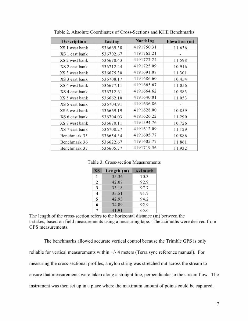
Table 2. Absolute Coordinates of Cross-Sections and KHE Benchmarks

Description Easting Northing Elevation (m) XS 1 west bank 536669.38 4191750.31 11.636 XS 1 east bank 536702.67 4191762.21 - XS 2 west bank 536670.43 4191727.24 11.598 XS 2 east bank 536712.44 4191725.09 10.916 XS 3 west bank 536675.30 4191691.07 11.301 XS 3 east bank 536708.17 4191686.60 10.454 XS 4 west bank 536677.11 4191665.67 11.056 XS 4 east bank 536712.61 4191664.62 10.583 XS 5 west bank 536662.10 4191640.01 11.053 XS 5 east bank 536704.91 4191636.86 - XS 6 west bank 536669.19 4191628.00 10.859 XS 6 east bank 536704.03 4191626.22 11.290 XS 7 west bank 536670.11 4191594.76 10.726 XS 7 east bank 536708.27 4191612.09 11.129 Benchmark 35 536654.34 4191605.77 10.886 Benchmark 36 536622.67 4191605.77 11.861 Benchmark 37 536605.77 4191719.56 11.932

Table 3. Cross-section Measurements

XS Length (m) Azimuth 1 35.36 70.3 2 42.07 92.9 3 33.18 97.7 4 35.51 91.7 5 42.93 94.2 6 34.89 92.9 7 41.91 65.6

The length of the cross-section refers to the horizontal distance (m) between the t-stakes, based on field measurements using a measuring tape. The azimuths were derived from GPS measurements.

The benchmarks allowed accurate vertical control because the Trimble GPS is only

reliable for vertical measurements within +/- 4 meters (Terra sync reference manual). For

measuring the cross-sectional profiles, a nylon string was stretched out across the stream to

ensure that measurements were taken along a straight line, perpendicular to the stream flow. The

instrument was then set up in a place where the maximum amount of points could be captured,

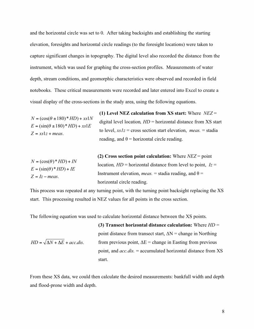
8

and the horizontal circle was set to 0. After taking backsights and establishing the starting

elevation, foresights and horizontal circle readings (to the foresight locations) were taken to

capture significant changes in topography. The digital level also recorded the distance from the

instrument, which was used for graphing the cross-section profiles. Measurements of water

depth, stream conditions, and geomorphic characteristics were observed and recorded in field

notebooks. These critical measurements were recorded and later entered into Excel to create a

visual display of the cross-sections in the study area, using the following equations.

(cos( 180)* ) 1

(sin( 180)* ) 1

1 .

N HD xs N

E HD xs E

Z xs z meas

!

!

= ± +

= ± +

= +

(1) Level NEZ calculation from XS start: Where NEZ =

digital level location, HD = horizontal distance from XS start

to level, xs1z = cross section start elevation, meas. = stadia

reading, and θ = horizontal circle reading.

(cos( )* )

(sin( )* )

.

N HD IN

E HD IE

Z Iz meas

!

!

= +

= +

= "

(2) Cross section point calculation: Where NEZ = point

location, HD = horizontal distance from level to point, Iz =

Instrument elevation, meas. = stadia reading, and θ =

horizontal circle reading.

This process was repeated at any turning point, with the turning point backsight replacing the XS

start. This processing resulted in NEZ values for all points in the cross section.

The following equation was used to calculate horizontal distance between the XS points.

. .HD N E acc dis= ! + ! +

(3) Transect horizontal distance calculation: Where HD =

point distance from transect start, ΔN = change in Northing

from previous point, ΔE = change in Easting from previous

point, and acc.dis. = accumulated horizontal distance from XS

start.

From these XS data, we could then calculate the desired measurements: bankfull width and depth

and flood-prone width and depth.

9

Results

Using the foresight, backsight, and horizontal circle measurements, the elevation of data

points was calculated and graphed with the corresponding point’s distance from the starting point

to show the elevation profile [Appendix B]. The x-axis shows the distance from the start of the

cross-section (meters) and the y-axis is the corresponding elevation (meters). The corresponding

UCB cross-sections are shown for reference and visual analysis [Appendix C]. Due to the

inability to accurately define starting and ending locations for the cross-sections, quantifiable

changes cannot be calculated. However, since the NPS strongly suggested using this study for

comparison, the graphs are included for potential qualitative analyses.

Discussion of Uncertainty:

Major sources of uncertainty in this study included the difficulty of re-occupying cross-

sections from the UCB 2007 survey and comparing 2008 results with previous data. As the UCB

survey lacked information about the absolute positions of each cross-section, the current cross-

sections do not entirely align with those of the UBC survey. In addition, since the UBC survey

did not capture an adequate amount of significant points along cross-sections, it was difficult to

quantify changes that have occurred in stream morphology over the past year. However,

qualitative analyses can be performed for the five cross-sections that roughly re-occupy similar

locations. To avoid this problem in the future, current cross-sections are clearly established with

documented locational data. In addition, the 2008 surveys were able to capture stream

morphology in detail; therefore, future studies will be able to replicate this study and detect

changes over time.

The consideration of timing and season of the survey is important for stream geomorphic

studies. All of the cross-sectional surveys were conducted over two days after the first rainfall

10

occurred. Though results clearly showed cross-sectional stream features, such as bankfull edges,

water depth, and thalweg, these features might not have been evident if the surveys were

conducted before the first rainfall events. In fact, before the first rainfall the Upper Alley reach of

Redwood Creek was a series of disconnected pools rather than one connected flowing stream. In

addition, the surveys might show or detect more significant results in the spring, as the creek

would receive a greater amount of water from the rainy season and possible effective discharge

events.

Although the maximum accuracy of instruments induced some measurement errors, the

magnitude of these errors seemed insignificant and negligible for the overall validity of this

study’s purpose and results. For instance, a Trimble GPS recorded the absolute locations of

starting points of cross-sections with accuracy of ± 0.5 m. However, this error was adequately

compensated by the facts that the averages of 40+ points were used and a digital level measured

relative positions from benchmarks. In addition, the vertical accuracy of the digital level (± 1

mm) was considered to be adequate for our study.

Some human induced errors might be associated with measurement and recording errors.

Though cross-sectional profiles were created based on measurements by a digital level, a

measuring tape also measured the length of each cross-section to assess the horizontal accuracy

of the digital measurements and calculations. Although the results indicated some horizontal

inaccuracy with our calculations, the magnitude of this error was considered to be insignificant

as the vertical accuracy was significantly more important for our cross-sectional surveys.

Moreover, setting up a straight transect was difficult along some cross-sections due to vegetation

covers and that cross-sections might not have been entirely perpendicular to the stream flow.

11

However, this error also seemed negligible for this study as results adequately showed cross-

sectional profiles in detail.

Conclusion

A geomorphic assessment of Redwood Creek was performed using level surveying and

physical geography methods. The overall accomplishments of this study included: determination

of horizontal and vertical controls, establishment of seven cross-sections with t-stakes for

starting and ending points, and the measurement and mapping of six cross-sections in the

restored section of the Creek, interspersed between the ELJs. Although the impacts of the ELJs

on stream morphology could not be quantified, future measurements could be taken along the

same cross-section locations to assess geomorphic changes to the channel over time by using the

methods and benchmarks provided in this study.

In order to evaluate the effects of the restoration project on the geomorphology of the

creek, it is recommended that future measurements be taken at least once a year, ideally post-

effective discharge events, following recommended criteria (Levell & Chang 2008). Woolsey et

al. (2008) recommends post-project evaluations of up to ten years before restoration projects are

declared successes or failures (Woolsey et al. 2007). For future studies, it is also recommended

that the procedure for obtaining a research permit is started well in advance because the process

can take awhile. As mentioned above, timing or season of surveys can significantly impact the

results, so that the careful consideration about when to do surveys should be taken.

This study contributes to the recorded data about Redwood Creek and identifies

recommended methods and criteria for future evaluation at this site. Hopefully, this study will

provide useful information and methodological foundation to the NPS and future surveys will be

performed to determine how the creek is changing. Continual monitoring can ensure that

12

adaptive management practices can be employed to effectively manage the creek and enhance

salmonid habitat in this critical environment.

References

Abbe, T., Brooks, A., and Montgomery, D. 2003. Wood in River Rehabilitation and Management. In American Fisheries Society Symposium, 367-390. American Fisheries Society. Flosi, G., Downie, S. Hopelain, J. Bird, M., Coey, R. and Collins, B. 1998. California Salmonid Stream Habitat Restoration Manual. State of California, The Resources Agency, California Dept. of Fish and Game, Inland Fisheries Division. Golden Gate National Recreation Area (GGNRA). 2002. Environmental Assessment Lower Redwood Creek interim flood reduction measures and floodplain/channel restoration. 55 pp. Prepared for the National Park Service. [online] http://www.krisweb.com/biblio/southmarin_goga_staff_2002_redwoodcrkeafinal.pdf [last accessed 16 December, 2008]. _____________ 2007. Environmental Assessment Lower Redwood Creek Floodplain and Salmonid Habitat Restoration, Banducci Site. March 2007. Prepared for the National Park Service. Kamman Hydrology & Engineering, Inc. (KHE). 2007. Design Report for Lower Redwood Creek Floodplain and Salmonid Habitat Restoration at the Banducci Site. Prepared for the Golden Gate National Parks Conservancy and the National Park Service. San Francisco, California, 105 pgs. Kondolf, G.M.1995. Five elements for effective evaluation of stream restoration. Restoration Ecology 3: 133-136. Kondolf, G.M., E.R. Micheli. 1995. Evaluating stream restoration projects. Environmental Management 19: 1-15. Levell, A.P., H. Chang. 2008. Monitoring the Channel Process of a Stream Restoration Project in an Urbanizing Watershed: A Case Study of Kelly Creek, Oregon, USA. River Restoration Applications 24: 169-182. Marin Municipal Water District (MMWD). 2008. Rainfall History Lake Lagunitas. [online] http://www.marinwater.org/documents/RAINFALL_HISTORY_as_2008.pdf [last accessed 16 December 2008]. Philip Williams & Associated (PWA). 2000. The Feasibility of Restoring Floodplain and Riparian Ecosystem Processes on the Banducci Site, Redwood Creek. Prepared for the Golden Gate National Recreation Area, San Francisco, California, October, 69 pp. ____________. 2002. Preliminary design report, lower Redwood Creek restoration project. Prepared for: The National Parks Service, Golden Gate National Recreation Area, April, 45p.

13

Woolsey, S., F. Capelli, T. Gonser, E. Hoehn, M. Hostmann, B. Junker, A. Paetzold, C. Roulier, S. Schweizer, S.D. Teigs, K. Tockner, C. Weber, A. Peter. 2008. A strategy to assess river restoration success. Freshwater Biology 52: 752-769.