IZA DP No. 2548

Exploring the Impact of Interrupted Educationon Earnings: The Educational Cost of theChinese Cultural Revolution

Xin MengRobert Gregory

DI

SC

US

SI

ON

PA

PE

R S

ER

IE

S

Forschungsinstitutzur Zukunft der ArbeitInstitute for the Studyof Labor

January 2007

Exploring the Impact of

Interrupted Education on Earnings: The Educational Cost of the Chinese Cultural Revolution

Xin Meng Australian National University

and IZA

Robert Gregory Australian National University

and IZA

Discussion Paper No. 2548 January 2007

IZA

P.O. Box 7240 53072 Bonn

Germany

Phone: +49-228-3894-0 Fax: +49-228-3894-180

E-mail: iza@iza.org

Any opinions expressed here are those of the author(s) and not those of the institute. Research disseminated by IZA may include views on policy, but the institute itself takes no institutional policy positions. The Institute for the Study of Labor (IZA) in Bonn is a local and virtual international research center and a place of communication between science, politics and business. IZA is an independent nonprofit company supported by Deutsche Post World Net. The center is associated with the University of Bonn and offers a stimulating research environment through its research networks, research support, and visitors and doctoral programs. IZA engages in (i) original and internationally competitive research in all fields of labor economics, (ii) development of policy concepts, and (iii) dissemination of research results and concepts to the interested public. IZA Discussion Papers often represent preliminary work and are circulated to encourage discussion. Citation of such a paper should account for its provisional character. A revised version may be available directly from the author.

IZA Discussion Paper No. 2548 January 2007

ABSTRACT

Exploring the Impact of Interrupted Education on Earnings: The Educational Cost of the Chinese Cultural Revolution*

During the Chinese Cultural Revolution many schools stopped normal operation for a long time, senior high schools stopped student recruitment for up to 6 years, and universities stopped recruitment for an even longer period. Such large scale school interruptions significantly reduced the opportunity for a large cohort of individuals to obtain university degrees and senior high school qualifications. More than half of this cohort who would normally attain a university degree were unable to do so. We estimate that those who did not obtain a university degree, because of the Cultural Revolution, lost an average of more than 50 percent of potential earnings. Both genders suffered reduced attainment of senior high school certificates and more than 20 per cent prematurely stopped their education process at junior high school level. However, these education responses do not appear to have translated into lower earnings. In addition, at each level of education attainment most of the cohort experienced missed or interrupted schooling. We show, however, that given the education certificate attained, the impact on earnings of these missed years of schooling or lack of normal curricula was small. JEL Classification: I21, J31 Keywords: education, earnings, Cultural Revolution, China Corresponding author: Xin Meng Division of Economics Research School of Pacific and Asian Studies Australian National University Canberra 0200 Australia E-mail: Xin.Meng@anu.edu.au

* We would like to thank conference participants at the European Population Economics Annual Conference, 2001 and seminar participants at the Australian National University, and the Universities of Aberdeen, Stirling, and Western Sydney for helpful comments.

1 Introduction

In 1966, the Chinese Communist Party began a political event–the Cultural Revolution (CR)–

during which most urban schools in China ceased normal operation for a long time, senior

high schools stopped student recruitment for up to 6 years, while universities stopped student

recruitment for an even longer period (Unger, 1982 and Meng and Gregory, 2002). Over the

entire course of the 11-years of the Cultural Revolution a generation of urban young people

was affected in terms of school outcomes. Some cohort groups missed as much as 4 to 6 years

of schooling. Many individuals missed a chance to obtain a university degree or a senior high

school qualification.

The question naturally arises as to how such large scale school interruptions affect lifetime

earnings. Recent development of an IV-LATE approach (see, for example, Angrist, Imbens,

and Rubin, 1996) provides a useful tool to examine this question. Ichino and Winter-Ebmer

(2004) using this approach found, for a number of European countries, that those individuals

who would have obtained higher education, but because of World War II did not, suffered a

considerable loss of earnings. The Cultural Revolution experience can add a new dimension to

this literature.

The emphasis of this paper is on two issues. First, the extent to which the interrupted edu-

cation in urban China during the Cultural Revolution affected subsequent education attainment

of the cohort (referred to as the Interrupted Education Cohort, IE cohort, or IEC, hereafter).1

Second, the impact of interrupted education on subsequent earnings of the IE cohort in the

1990s and early 2000s due to the lack of educational achievement.2

The paper is structured as follows: Section 2 provides background on the education disrup-

tions of the Cultural Revolution, defines the control groups, and discusses the data. Section 3

investigates the effect of the Cultural Revolution on educational attainment. Section 4 exam-

ines the earnings’ effect of school interruptions. Section 5 pulls the various parts of the study

together to investigate the long term cost of the interrupted education due to the Cultural

1The precise definition of the Interrupted Education Cohort (IE cohort) is given in Section 2.2 Individual earnings in the pre-economic reform era (before 1978) were administratively determined and this

situation did not significantly change until the later stages of economic reform in the 1990s (Meng, 2000). Hence,the focus of this paper is on earnings of individuals during 1992 to 2002 period.

2

Revolution. Section 6 offers concluding comments.

2 Background and data

2.1 Background

Just before the Cultural Revolution, the structure of the school system in urban China varied

slightly from city to city. The usual pattern was that students began formal schooling at age 7,

followed by six years of primary school, three years of junior high and three years of senior high

school (Deng and Treiman, 1997, Meng and Gregory, 2002). There were three degree types;

a 4-year full-time degree, a 3-year full-time degree and a degree by correspondence or night

school. The latter two degrees are regarded as the same in the labour market and all surveys

group them together. We refer to them as semi-degrees.

The Cultural Revolution profoundly disrupted this urban education system. The history

can be divided into four overlapping time periods.

The first period extends from the beginning of the Cultural Revolution in 1966 to 1968.

No formal teaching was carried out in the urban education system and no new students were

recruited to education institutions. It was usual for primary school age students to stay at

home3 and for junior and senior high school and university students to meet each day at school

to undertake political activities. These were the peak years of education disruption.

The second period begins around 1968—1969 when primary and junior high school education

recommenced. Those, who under normal circumstances would have completed primary school

during 1966—1968 could go on to junior high schools. Children aged 7—9 could begin primary

school. However, teachers were not allowed to follow standard curricula. Instead, students spent

much of their school time going to factories and the countryside to do manual work. It was not

3 It is not completely clear how many primary schools were closed in urban areas. Deng and Treiman (1997) citeUnger (1982) and Bernstein (1977) to claim that most primary schools continued to operate as usual during thefirst two years of the Cultural Revolution. This does not appear to be the case in the majority of urban areas whereprimary schools were closed and students stayed at home or went to school but without any formal education.Deng and Treiman (1997) appear to have misinterpreted Unger (1982). In his book Unger explicitly states "In asmuch as two years had passed since classes had been temporarily suspended at the Cultural Revolution’s start,three years’worth of children would enter the first grade of primary school in the autumn of 1968." (Unger, 1982,p274). In addition, as almost all students who returned to junior high school in 1968 had been primary schoolstudents in 1966, he states that “They had been out on the streets running wild for two years, and many of themwere little inclined to return passively to their school desks” (Unger, 1982, pp.149).

3

until 1970 that normal curricula were gradually resumed at primary and junior high schools.

During this period, formal education at senior high schools continued to be suspended.

Those who were in junior or senior high school at the beginning of the Cultural Revolution were

given qualifications at the normal graduation age, even though they had missed various years

of standard schooling. Some of this group, and new graduates from junior high schools, were

sent to the countryside to become peasants or to work in factories. Others were given jobs in

the city or in the army.

The third period begins from 1972 when senior high schools began recruiting new students

directly from junior high school. Those who had missed senior high school, as a result of the

Cultural Revolution, were not allowed to return to the high school system. After the Cultural

Revolution, however, many were able to obtain senior high school certificates by correspondence

or at night school. From around this time the standard school curricula was gradually resumed

throughout the school system, although factory and farm work was retained as an important

part of the curricula, especially in high schools.

Education disruption at university level extended over a longer period. No standard univer-

sity teaching or recruitment was undertaken from 1966 to 1970—71. Those who began university

before the Cultural Revolution, and had not completed their degrees, were allowed to stay at

university without formal teaching until 1970—71. They were then given their degree and as-

signed jobs usually as schoolteachers, factory workers, or army recruits.

From 1972, universities began restricted and small-scale recruitment, based upon political

attitudes or family background rather than on academic merit. New students were drawn only

from those who were workers, peasants, or soldiers. New senior high school graduates were not

allowed to proceed to university directly. They were sent to the countryside or assigned jobs.

The quality of university education dropped as a result of lower student intake quality and

lack of qualified lecturers and professors, many of whom had been sent to the countryside for

re-education. In recognition of this quality reduction, the authorities now also refer to degrees

acquired during this period as semi-degrees.

The final period began when the Cultural Revolution ended in 1977, and extends until 1981.

During 1977, universities returned to normal, resumed entrance exams and began recruiting on

4

academic merit. Everyone who had missed a chance to go to university because of the Cultural

Revolution was entitled to sit entrance exams. Thus, the accumulation of eleven years of

candidates began to compete with new senior high school graduates for a limited number of

positions. This lasted for four years until 1981, when those who were older than twenty-five years

of age were excluded from university entrance. The Interrupted Education Cohort, however,

could still acquire semi-degrees by correspondence.

The best data for interrupted education during this period would be the details of the actual

education experience of each individual in our sample but these data are not available. However,

to the best of our knowledge, the education interruption during the Cultural Revolution is closely

associated with an individual’s date of birth.

The assumed relationship between birth date and interrupted education is presented in Table

1 which summarises the level and number of school years interrupted for each birth cohort group

and the age at which university entrance was a possible choice. Although school years missed,

and years at school without normal curricula, are slightly different, our analysis suggests that

they may be grouped together as one variable which we label as interrupted education (Meng

and Gregory, 2002). Thus, the interrupted education in Table 1 includes both school years

missed and years at school but without normal curricula periods.

Table 1 indicates that about 15 urban cohort groups were affected by missed schooling, or

lack of normal curricula. These cohorts were aged between 5 and 19 years when the Cultural

Revolution began in 1966 (those born between 1947 and 1961). Some cohorts missed all six

years of junior and senior high school. Some missed many years of primary schooling and others

missed various combinations of primary, junior and senior high school. Missed schooling was

most serious for middle cohort groups. These 15 cohort groups form the Interrupted Education

Cohort (IE cohort).

2.2 Defining control groups

Our analytical purpose is two fold. First, we seek to evaluate the effect of interrupted education,

due to the Cultural Revolution, on subsequent education attainment. Second, we evaluate the

effect of interrupted education, through the change in education attainment, on earnings later

5

in life.

In the first instance, the outcome is the highest level of education certificate attained or

years of schooling achieved and the treatment is education disruption due to the Cultural Rev-

olution. As selection into treatment (whether an individual belongs to the IE cohort) is based

on birth cohort, which is exogenous, the evaluation of the change in education attainment can

be estimated using OLS. In the second instance, the outcome is earnings and the treatment is

educational attainment. Because selection into treatment in this instance is not exogenous, an

IV estimate is required. The instrument used is the IE cohort dummy, which is exogenous.

For our purpose it is convenient to interpret the IV estimates as a Local Average Treatment

Effect (LATE) (see Imbens and Angrist, 1994; Angrist and Imbens, 1995; and Angrist, Imbens,

and Rubin, 1996). The IV/LATE estimates indicate the earnings loss for individuals of the

IE cohort whose education was reduced because of interrupted education during the Cultural

Revolution. Detailed discussion as to the estimation and interpretation of the education and

earnings equations will be provided in Sections 3 and 4. Here the focus is mainly on the choice

of control groups.

The effect of interrupted education on an outcome, α, can be defined as:

α = E(Y 1 − Y 0) (1)

where Y 1 is the observed outcome for the treatment group (IE cohort) and Y 0 is the “would-

have-been” outcome had the Cultural Revolution not interrupted education of the cohort. For

each individual in the treatment group we observe Y 1 but not Y 0 and a control group is needed

to calculate Y 0. The control group should be as similar to the treatment group as possible,

except for the treatment. In particular, the control group must have experienced the Cultural

Revolution and be affected in the same way as the IE cohort, except for education interruption.

In natural experiments it is not possible to find a perfect control group and we are in a similar

position as other researchers who use this technique. We explore two possible control groups,

each with particular strengths and weaknesses. The first control group is an urban before-

after group which includes those who were born between 1942 and 1946 (the before group)

6

and those who were born between 1962 and 1966 (the after group). The before group started

their education after the communists took power in 1949 and completed their education under

the same communist system as our treatment group. When the Cultural Revolution began

they were 20 to 24 years old and had already finished schooling or entered university4 and did

not experience interrupted education. The after group experienced the Cultural Revolution in

their early life but when the oldest of this group was at primary school entry age in about

1969, schools were open and soon restored the standard school curricula. When the Cultural

Revolution ended the youngest of the after group was around 10 and the oldest around 14 years

of age.

The strength of the before-after control group is that they lived in urban areas and experi-

enced a similar economic environment, education system, and general Cultural Revolution effect

as the treatment group, except for interrupted schooling. We choose a narrow birth cohort range

(5 years before and 5 years after the IE cohort) to increase the probability that control and

treatment groups share similar experiences. Nevertheless, treatment and control groups were

at different ages when the Cultural Revolution occurred and this may be a weakness. More

formally, the outcome, Y 1 and Y 0 for the urban IE cohort and control groups may be defined

as:

Y 1U = α+AGEIEC +EU +X and Y 0U = AGENIEC +EU +X (2)

where α is the effect of interrupted education due to the Cultural Revolution, AGEIEC and

AGENIEC are any age specific Cultural Revolution effect (such as psychological effect of the

political turmoil) particularly related to the treatment (IEC) and control groups (NIEC), respec-

tively. EU is any general Cultural Revolution effect which applies to everybody from the urban

sector who experienced the Cultural Revolution and X is a vector of other relevant variables.

The difference between the two groups provides:

4Those who began university before the Cultural Revolution, and had not completed their degrees at the timethe Cultural Revolution started, were given their degree and assigned jobs in 1970-1971. Thus, the qualificationattained by this group are not affected by "Interrupted Education" as defined in this study.

7

Y 1U − Y 0U = α+∆AGE (3)

where ∆AGE = AGEIEC −AGENIEC , refers to any difference in age specific Cultural Revolu-

tion effects between control and treatment groups. Thus, with this control group the evaluation

may measure both the effect due to interrupted education and an age specific Cultural Rev-

olution effect. If this is the case, the ignorability assumption for interpreting the IV earnings

equation as LATE would be violated. However, by narrowing the before-after group to a small

range of birth cohorts we hope to minimise possible contamination from this source and in

Section 4 we also explicitly check whether ∆AGE > 0.

Another possible control group is a rural sample. The Cultural Revolution affected the

general political, economic, and social environment of both urban and rural areas, but large-

scale school interruption did not generally occur in rural areas. Although no official documents

have been found to record the history of school closures, conventional wisdom is that rural

schools suffered much less disruption than urban schools.5 Our data, presented later, show that

unlike urban workers, the education level of the rural IE cohort (the cohort born between 1947

and 1961) does not appear to have been significantly affected.

The strength of the rural control group is that it allows comparison of age groups, which

exactly match each age cohort of the urban before-after control and each age cohort of the

treatment groups, but the rural “treatment group” was not treated (did not experience large

5Documented information on rural schools’ responses during the Cultural Revolution is difficult to find. Theauthors communicated with Professor Jon Unger, who is the author of the first and classic book discussingschooling during the Cultural Revolution. He indicated that he collected a large quantity of materials andinterview records about rural schooling during the Cultural Revolution. Unfortunately due to word limits he didnot put these materials into his book. His materials suggest that large scale school interruption did not occurin rural areas. Schools, especially primary schools, were mostly open during the first few years of the CulturalRevolution while their counterparts in urban areas were closed. Regarding junior and senior high schools, hisimpression was that in the commune headquarter towns, where the only high schools were located, sometimesthese were closed during 1967 and in the first half of 1968 if the Cultural Revolution was active there. In addition,Andreas (2004) includes a table (Table 4) of new student enrollment for all of China in regular junior high schools,which indicates that in 1965 (one year before the Cultural Revolution begun), the total number of new ruralenrollments was 1,719,000, while urban area enrollments were 1,279,000. In 1967 the split of rural/urban newenrollment data are not available, but the total enrollment number is 1,983,000, slightly higher than the ruralenrollment number in 1965. Given that neither junior nor senior high schools in urban areas started recruitmentuntil 1968 (Unger, 1982; Deng and Treiman, 1997; Meng and Gregory, 2002) we may assume that the majority ofthe total new enrollments was in rural areas and therefore large scale prolonged school interruption was absent,although short term disruptions may have occurred in some areas, where the Cultural Revolution was active.

8

scale school interruptions) or was treated at a much lower level (school interruption for a short

time in some areas). Formally, the outcomes for the rural IE cohort and the rural before-after

cohorts may be defined as:

Y 1R = eα+AGEIEC +ER+X, and Y 0R = AGENIEC +ER+X (4)

where eα is the interrupted education effect for the rural population and 0 5 eα < α and ER

indicates any general Cultural Revolution effect. The difference between the two outcomes for

the rural sample is Y 1R−Y 0R = eα+∆AGE, which is similar to equation (3). On the assumptionthat any age specific Cultural Revolution effects, which is not related to interrupted education,

are the same in rural and urban areas the difference-in-differences estimate is:

(Y 1U − Y 0U )− (Y 1R − Y 0R) = α− eα (5)

which may allow us to remove any age specific Cultural Revolution effects. However, a by-

product of this approach is that the difference-in-differences result may be contaminated if

eα > 0, that is schools were closed in rural areas. If that is the case, the estimate from equation

(5) should be an underestimate. As indicated earlier, we believe large scale school interruptions

did not occur in rural areas, and hence, eα should be very small, if not zero (see footnote 5).There are other problems, however, from using the rural sample as a control group. First,

very few rural workers have above senior high school qualifications. Thus, the effective com-

parison with the urban sample is limited to pre-university schooling only. Second, most rural

workers are self-employed rather than wage earners, and hence, only a relatively small sample

of rural wage earners is available as a control group and there may be a sample selection bias.6

Considering the strengths and weaknesses of both control groups, our strategy is to place

most emphasis on the urban before-after control group but to use both control groups as much

as possible and to use the findings from each to reach the best possible judgement as to the

6Of course, there may be other problems. Rural and urban workers may have very different family backgroundsand other systematic differences. However, it is unlikely that such differences will differ between cohorts whichexperienced education interruptions during the Cultural Revolution and those who did not (before-after cohort).Thus, a difference-in-differences approach should allow us to remove family background differences and any othersystematic differences between rural and urban samples.

9

interrupted education effect of the Cultural Revolution on subsequent earnings. In all natural

experiments some component of individual judgement as to the degree of validity of the control

groups is unavoidable.

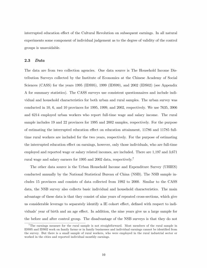
2.3 Data

The data are from two collection agencies. One data source is The Household Income Dis-

tribution Surveys collected by the Institute of Economics at the Chinese Academy of Social

Sciences (CASS) for the years 1995 (IDS95), 1999 (IDS99), and 2002 (IDS02) (see Appendix

A for summary statistics). The CASS surveys use consistent questionnaires and include indi-

vidual and household characteristics for both urban and rural samples. The urban survey was

conducted in 10, 6, and 10 provinces for 1995, 1999, and 2002, respectively. We use 7635, 3906

and 6214 employed urban workers who report full-time wage and salary income. The rural

sample includes 19 and 22 provinces for 1995 and 2002 samples, respectively. For the purpose

of estimating the interrupted education effect on education attainment, 11786 and 11785 full-

time rural workers are included for the two years, respectively. For the purpose of estimating

the interrupted education effect on earnings, however, only those individuals, who are full-time

employed and reported wage or salary related incomes, are included. There are 1,197 and 3,671

rural wage and salary earners for 1995 and 2002 data, respectively.7

The other data source is the Urban Household Income and Expenditure Survey (UHIES)

conducted annually by the National Statistical Bureau of China (NSB). The NSB sample in-

cludes 15 provinces and consists of data collected from 1992 to 2000. Similar to the CASS

data, the NSB survey also collects basic individual and household characteristics. The main

advantage of these data is that they consist of nine years of repeated cross-sections, which give

us considerable leverage to separately identify a IE cohort effect, defined with respect to indi-

viduals’ year of birth and an age effect. In addition, the nine years give us a large sample for

the before and after control group. The disadvantage of the NSB surveys is that they do not

7The earnings measure for the rural sample is not straightforward. Most members of the rural sample inIDS95 and IDS02 work on family farms or in family businesses and individual earnings cannot be identified fromthe survey. But there is a small sample of rural workers, who were employed in the rural industrial sector orworked in the cities and reported individual monthly earnings.

10

include a rural sample.

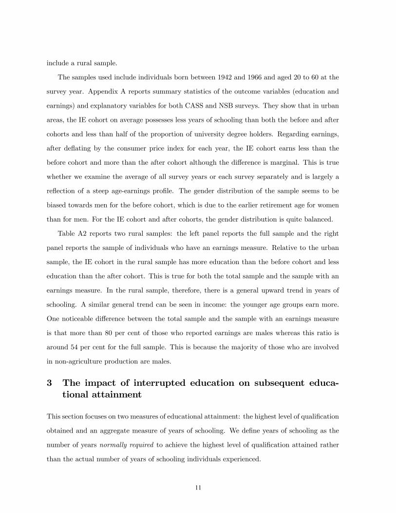
The samples used include individuals born between 1942 and 1966 and aged 20 to 60 at the

survey year. Appendix A reports summary statistics of the outcome variables (education and

earnings) and explanatory variables for both CASS and NSB surveys. They show that in urban

areas, the IE cohort on average possesses less years of schooling than both the before and after

cohorts and less than half of the proportion of university degree holders. Regarding earnings,

after deflating by the consumer price index for each year, the IE cohort earns less than the

before cohort and more than the after cohort although the difference is marginal. This is true

whether we examine the average of all survey years or each survey separately and is largely a

reflection of a steep age-earnings profile. The gender distribution of the sample seems to be

biased towards men for the before cohort, which is due to the earlier retirement age for women

than for men. For the IE cohort and after cohorts, the gender distribution is quite balanced.

Table A2 reports two rural samples: the left panel reports the full sample and the right

panel reports the sample of individuals who have an earnings measure. Relative to the urban

sample, the IE cohort in the rural sample has more education than the before cohort and less

education than the after cohort. This is true for both the total sample and the sample with an

earnings measure. In the rural sample, therefore, there is a general upward trend in years of

schooling. A similar general trend can be seen in income: the younger age groups earn more.

One noticeable difference between the total sample and the sample with an earnings measure

is that more than 80 per cent of those who reported earnings are males whereas this ratio is

around 54 per cent for the full sample. This is because the majority of those who are involved

in non-agriculture production are males.

3 The impact of interrupted education on subsequent educa-tional attainment

This section focuses on two measures of educational attainment: the highest level of qualification

obtained and an aggregate measure of years of schooling. We define years of schooling as the

number of years normally required to achieve the highest level of qualification attained rather

than the actual number of years of schooling individuals experienced.

11

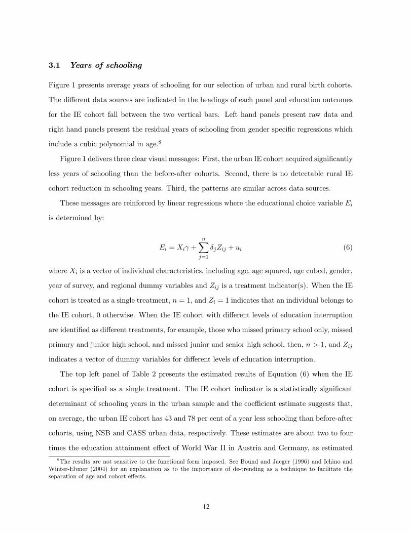
3.1 Years of schooling

Figure 1 presents average years of schooling for our selection of urban and rural birth cohorts.

The different data sources are indicated in the headings of each panel and education outcomes

for the IE cohort fall between the two vertical bars. Left hand panels present raw data and

right hand panels present the residual years of schooling from gender specific regressions which

include a cubic polynomial in age.8

Figure 1 delivers three clear visual messages: First, the urban IE cohort acquired significantly

less years of schooling than the before-after cohorts. Second, there is no detectable rural IE

cohort reduction in schooling years. Third, the patterns are similar across data sources.

These messages are reinforced by linear regressions where the educational choice variable Ei

is determined by:

Ei = Xiγ +nX

j=1

δjZij + ui (6)

where Xi is a vector of individual characteristics, including age, age squared, age cubed, gender,

year of survey, and regional dummy variables and Zij is a treatment indicator(s). When the IE

cohort is treated as a single treatment, n = 1, and Zi = 1 indicates that an individual belongs to

the IE cohort, 0 otherwise. When the IE cohort with different levels of education interruption

are identified as different treatments, for example, those who missed primary school only, missed

primary and junior high school, and missed junior and senior high school, then, n > 1, and Zij

indicates a vector of dummy variables for different levels of education interruption.

The top left panel of Table 2 presents the estimated results of Equation (6) when the IE

cohort is specified as a single treatment. The IE cohort indicator is a statistically significant

determinant of schooling years in the urban sample and the coefficient estimate suggests that,

on average, the urban IE cohort has 43 and 78 per cent of a year less schooling than before-after

cohorts, using NSB and CASS urban data, respectively. These estimates are about two to four

times the education attainment effect of World War II in Austria and Germany, as estimated

8The results are not sensitive to the functional form imposed. See Bound and Jaeger (1996) and Ichino andWinter-Ebmer (2004) for an explanation as to the importance of de-trending as a technique to facilitate theseparation of age and cohort effects.

12

by Ichino and Winter-Ebmer (2004). For the rural sample we find no statistically significant IE

cohort effect on years of schooling. If we combine the urban and rural sample and include an

urban dummy variable and an interaction term between it and the IE cohort dummy variable

we find that the difference-in-differences estimate indicates 83 per cent of a year less schooling

for the urban IE cohort.9

Table 2 also shows that school interruptions at every level of schooling (multiple treatments)

had significant impacts on years of schooling achieved by the urban population (top right panel).

Those who experienced interrupted junior and senior high school were most affected, acquiring

0.85 (NSB data) to 1.2 (CASS data) years less of schooling than before-after cohorts. Those

who missed primary school only, and those who did not miss any schooling, but were subject

to delayed university entry, were least affected. In general, the interrupted education effect on

school years completed is less for women than for men. Rural results, which are not reported,

are statistically insignificant as expected since rural students did not experience large scale

education interruption.

3.2 Highest level of qualification attained

Figure 2 presents highest level of qualification attained for each age cohort.10 Again there are

three clear visual messages.

The first visual message, evident in both data sources, is that the IE cohort has a noticeable

lower incidence of four-year degrees, relative to the before-after cohorts. The education regres-

sion model applied to whether an individual has a university degree or not (middle left panel

of Table 2) produces a highly significant coefficient attached to the IE cohort indicator (single

treatment), indicating that the IE cohort achieved a 5 to 7 percentage points lower four year

degree acquisition rate than the before-after cohorts. Furthermore, every level of interrupted

9Family background is an important determinant of individual educational attainment. However, in our dataonly a small sub-sample has information on parental years of schooling. We use this sub-sample to test if theinclusion of father and mother’s years of schooling changes our results and find that it reduces the estimatedreduction of school years for the IE cohort slightly but does not change the qualitative conclusions. For example,the estimated difference-in-difference result for the sample including parental information is a reduction of 0.65of a year schooling for the urban worker, and when parental information is excluded the reduction is 0.73 of aschool year. The full results including parental education variables are available upon request from the authors.10De-trended figures are consistent with Figure 2 but not reported here. They are available upon request from

the authors.

13

schooling (multiple treatments) had a significant and negative effect on university degree ac-

quisition (the middle right panel of Table 2). The largest effects were experienced by those

with interrupted junior and senior high school education and those with interrupted senior high

school only. Those with no interrupted schooling but with delayed university entry were least

affected.

A second message of Figure 2 is that although access to all degrees was limited in much the

same way, the Cultural Revolution does not appear to have had an adverse impact on semi-

degree acquisition. After the Cultural Revolution there was considerable take-up of semi-degree

courses that could be acquired by correspondence or part-time enrolment. The IE cohort used

these pathways to achieve three year degrees and the acquisition levels are similar to the before

cohort (Meng and Gregory, 2002). There are no statistically significant IE cohort effects for

three-year degrees and results are not presented.11 Regression results are also not reported for

the rural sample because very few rural residents possess university or three-year degrees.

A third visual message of Figure 2 is that there is a clear Cultural Revolution impact on

the acquisition of junior and senior high school certificates. Within urban areas there is a

decreased attainment of senior high school certificates and an increased attainment of junior

high school certificates for cohorts affected by senior high school closure (cohorts born during

1950 to 1955, which we refer to as the sub-IE cohort). The urban regression results indicate

a significantly negative sub-IE cohort effect for senior high school acquisition (the bottom left

panel of Table 2). Those with interrupted junior and senior high school are mostly affected with

16 to 17 percentage points less chance of obtaining a senior high school certificate (the bottom

right panel of Table 2). Those with interrupted senior high school only, experience a 11 to 14

percentage points reduction. All effects are statistically significant and once again the results

are consistent across data sources.12

11 It is noticeable that there is a significant increase in semi-degrees among post IEC cohorts, perhaps inresponse to enhanced opportunities presented by the growth of correspondence courses and the provision ofpart-time places.12Data on senior and junior high school trends in Figure 2 show that there is a large expansion of senior

high school in later cohorts (born between 1958 to 1960). At this stage we are not clear why this happened.Are our estimated results influenced by this expansion? To test this we exclude cohorts born after 1957 fromour sample. This restriction reduces the estimated effect of interrupted education only very slightly, with thosewith interrupted junior and senior high school having a 14 per cent less chance of obtaining a senior high schoolqualification and those with interrupted senior high school experiencing a 10 to 13 per cent reduction in senior

14

Rural outcomes are quite different and, as expected, there is no obvious IE cohort effect.

There is an increase in senior high school attainment among rural people towards the end of

the Cultural Revolution period that also occurs in the urban sample once senior high schools

re-opened.

To conclude, the evidence shows that education interruption associated with the Cultural

Revolution had widespread effects on urban years of schooling and certificate attainment relative

to the urban before-after control groups but no statistically detectable effect in rural areas.

Among the urban IE cohort, completed years of schooling fell between 43 and 78 per cent of a

year, acquisition of a university degree fell by about 5 to 7 percentage points and senior high

school attainment fell by 11 percentage points. Furthermore, the evidence provides direct links

between the level of schooling interrupted and education attainment. Perhaps, as might be

expected, the combination of interrupted junior and senior high school affects years of schooling

the most. With regard to university degree attainment all levels of school interruption have

similar effects.

4 The impact of interrupted education on subsequent earnings

Figure 3 presents real monthly earnings for employed full-time workers classified by birth cohort

and subject to a three year moving average to smooth the series. The strong downward trend

in the urban data is a product of the age earnings profile with the young birth cohorts earning

less than older cohorts. The earnings pattern of the much smaller rural sample reflects an age

earnings profile for a less skilled workforce subject to rapid technological change in that the

younger age groups earn more than older age groups.

To facilitate a preliminary glance at the data we regressed individual earnings, from each

data set, against a dummy variable for survey year and a cubic defined on age. While the

rural de-trended data exhibit no obvious pattern, the residual pattern of earnings for each

urban cohort reveals a consistent pattern across the two data sets. On average, the IE cohort

residuals are negative and particularly so for age groups subject to the interrupted primary

and junior high school, those born between 1956 and 1959. For these cohorts the residuals

high school attainment.

15

average around 2 to 4 per cent less than the before-after groups. Could these lower earnings

of IE cohort urban workers be attributed to reduced educational attainment as analysed in the

previous section?

The impact of reduced educational attainment on subsequent earnings depends on the eco-

nomic return to education. To estimate the average education-earnings link during our data

period, 1992-2002, we regress lnWi, log monthly earnings of individual i, against normal Mincer

type variables

lnWi = Xiβ +Eiα+ i (7)

where Ei indicates individual i’s educational attainment and X is the vector of exogenous

variables included in Equation (6). Equation (7), fitted by ordinary least squares, provides an

estimate of the average rate of return for different education levels. The OLS results from Table

5, for example, indicate that a male university graduate earns approximately 24 to 28 per cent

more than an average male without a university degree and a senior high school male graduate

earns around 14 to 17 per cent more than a male with less than a senior high qualification.

Across all education categories, male workers receive, on average, a 5 per cent wage premium

for each additional year of schooling. In all cases the education return for females is higher than

for males. These estimates are similar to those found in other studies based on Chinese data

over this period (Liu, Meng, and Zhang, 2000).

If we assume the rate of return to schooling is the same for the control and treatment

groups, we may combine the OLS estimates of average education returns with the reductions in

schooling estimated in the previous section to estimate the impact of education interruption on

individuals’ earnings. If, however, we assume the rate of return to schooling is different for the

treatment and control group but constant within each group, equation (7) may be estimated

with an interaction term between the IE cohort dummy and Ei, which provides an estimate

of the Average Treatment Effect (ATE). However, these average education returns may be

inappropriate if returns to schooling are different between treated individuals who responded

to the treatment (compliers) and those who did not (always takers and never takers), that is α

16

in equation (7) should have a subscript i.

To explore this issue we estimate the earnings effect of reduced education attainment due to

interrupted education by adopting the Local Average Treatment Effect (LATE) interpretation

of the instrumental variable approach proposed by Imbens and Angrist (1994), Angrist and

Imbens (1995), and Angrist, Imbens, and Rubin, (1996). To estimate the LATE we jointly

estimate the education equation (6) and the earnings equation (7) using an IV method. The IE

cohort dummy(ies) is(are) used as the instrument(s).

Before reporting the results we focus on some of the assumptions that must be satisfied to

legitimately interpret the IV estimate as a Local Average Treatment Effect (see Angrist, Imbens

and Rubin, 1996). Although it is not possible to fully test whether all assumptions are met we

took the following steps.

One important assumption is that if interrupted education due to the Cultural Revolution

affects IE cohort earnings this effect operates only through our education measures and there

should be no other channels through which interrupted education impacts on earnings (the

exclusion restriction). This restriction implies that for those whose schooling was not affected

by interrupted education there should be no change in earnings because of interrupted education.

For those whose schooling was affected by interrupted education the only source of lower earnings

should be the education change. There is no test to ensure that the exclusion restriction is fully

satisfied because we can never observe the counterfactual situation. However, we can build

confidence in the restriction by investigating possible sources of violation.

One possible source of violation arises because we measure Ei as the highest level of school

certificate attained, or as years of schooling which are calculated as the highest level of school

certificate attained adjusted by the school years normally required for each level. Given the

level of education certificate, however, years of schooling missed was not taken into account. For

example, those with a senior high school certificate who missed two or more years of schooling

are assumed to have the same years of schooling as those with a senior high school certificate

who completed all the required years. If those with more missed schooling years earned less, for

any given education attainment, the exclusion restriction would be violated.

To provide some indication of this possible violation we estimate separate earnings equations

17

for each education certificate level. These earnings equations include all variables from equation

(7) except Ei and include a variable indicating the number of years schooling missed.13 The

results are reported in Table 3. At each education certificate level (university, 3-year degree,

senior high, and junior high), missed school years do not significantly affect earnings, except for

the junior and senior high school certificates when using NSB data, where very small (0.002 and

0.005), positive, and statistically significant coefficients are obtained.14 Given the small size of

the coefficients (0.2 to 0.5 per cent of earnings) and that these effects are only found in one

data set, we assume that the effect of missed schooling on IE cohort earnings should mainly be

through our measure of Ei, the highest level of school certificate attained or calculated years

of schooling. The bias brought about by the possible violation of the exclusion restriction for

those with senior and junior high school certificates should be very small but should be borne

in mind when the results are discussed.

To further investigate whether we may meet the exclusion restriction, we estimate earnings

equations including an IE cohort dummy variable for urban and rural samples separately. The

results, listed in Table 4, indicate that for urban workers the IE cohort earns statistically

significantly less earnings than the before-after control group, if education variables are excluded

from the regressions. Once education variables are included, however, the education coefficients

are statistically significant but no statistically significant IE cohort effect is observed. For the

rural sample, the IE cohort dummy is not statistically significant with or without education

variables. These results suggest that there does not seem to be an obvious and substantial

interrupted education effect on earnings other than through its effect on education attainment.

Another important assumption required when interpreting the IV estimate as LATE is

that earnings of those subject to interrupted education should not be affected by other factors

which are different from but correlated with interrupted education (the ignorability assumption).

Our major concern is that there may be other age specific Cultural Revolution effects for the

IE cohort, which may adversely affect the earnings of this group independent of interrupted

13The years of schooling missed for each cohort are explained in Section 2.1 and Table 1.14Further investigation reveals that the positive and significant effects of missed schooling, given the certificate

level, are driven by the female sample. For males no significant effect is found at any certificate level. Hence, anybias is confined to the female results.

18

education. An example would be that everybody who went through the Cultural Revolution

would have experienced some kind of psychological shock, which might vary for different age

cohorts. We purposely chose the birth cohorts of the before-after control group to be as close

to our treatment group as possible so that any age specific Cultural Revolution effect are more

likely to be common across the treatment and before-after control groups.

However, one possible effect that stands out is that a large proportion of the IE cohort was

sent to the countryside for many years. This may have affected their health, as many were

working on farms for extended periods and the work was hard and the diet often limited. Farm

work also gave the cohort a different kind of work experience, which may have been less valuable

than non-agricultural work experience and may have affected subsequent earnings. The CASS

data identifies those who went to the countryside because of the Cultural Revolution and the

1999 and 2002 surveys also include self-assessed health information. Although the 1995 survey

did not include this question, it inquired as to the number of sick leave days taken during 1995.

We looked for any correlation between countryside experience and health or sick leave days and

failed to find a relationship. The earnings equation (7) was also estimated including a dummy

variable for “country work experience” but the coefficient is statistically insignificant.15

Given this background we now turn to the LATE estimates reported in Table 5, with the

top and bottom panels reporting results from CASS and NSB data, respectively.16 To test the

strength of the instrument(s), the F-Statistics for inclusion of the instrument(s) are presented at

the bottom row of each panel. The tests show that the instruments have very strong explanatory

power and that even considering the finite sample problem any bias from weak instruments

should be limited (Staiger and Stock, 1997). Since the estimated coefficients attached to other

variables appear to be similar to those found in the west, and similar to other studies based on

CASS data (Gustafsson and Li, 2000), the comments focus mainly on education results.17

The LATE estimates for acquisition of a university degree are listed in the first three columns

15There are other assumptions required to interpret IV estimate as LATE. For example, Monotonicity and theStable Unit Treatment Value Assumptions. For a detailed discussion, see Angrist, Imbens, and Rubin (1996).16Note that the adjusted R-Squared reported in Table 5 is often quite high. The important contributors to

the high R-squared are the wage variation across regions and over time, captured by regional and year dummyvariables.17The full results are available upon request from the authors.

19

titled “Below University” of Table 5. They indicate that male compliers (those who did not

obtain a university degree, just because of interrupted schooling during the Cultural Revolution)

experienced 46 to 51 per cent lower earnings and for female compliers the estimates are 73 to

76 per cent, using a single IE cohort dummy as an instrument. When five instruments are used

they provide a weighted average of the effects of different levels of education interruption on

earnings and produce similar but slightly lower results (Angrist and Imbens, 1995).

The earnings effect of reduced senior high school attainment of the sub-IE cohort are reported

in Columns 4 to 6 of Table 5 entitled “Below Senior High”. The IV estimates with one sub-

IE cohort dummy (those who were born between 1950 and 1955) as the instrument suggest

an average earnings loss for men of around 8 to 11 per cent although the estimate is only

significant when the NSB data are used. For women the estimated earnings effect is positive

but not statistically significant.

To provide an indication of the combined earnings effect of the reduction of university and

senior high school attainment, we estimate the LATE for years of schooling (Columns 7 to

9, entitled “Years of schooling”). When the single IE cohort dummy variable is used as an

instrument the estimated rate of return to an additional year of education is around 8 per cent

for males and 11 per cent for females. The weighted average rate of return using five instruments

are 4.5 to 4.7 per cent for an additional year of education for males and 3.0 to 5.5 per cent for

females.

We are now in a position to compare LATE and OLS estimates. There seems to be four

clear results (i) for four year university degrees the LATE estimates are very much larger than

the OLS estimates; (ii) for senior high school certificates the LATE are lower than the OLS

estimates–indeed in all but one instance not statistically different from zero; (iii) for years

of schooling the LATE estimates are larger when one instrument is used and lower when five

instruments are used, especially for women.

The difference between the OLS and the IV/LATE estimates suggest the difference between

the average rate of return for the sample as a whole and the average return for those in the

treated group who responded to the treatment (compliers). A particularly interesting aspect of

these results is the different impacts of interrupted education across education levels. We find

20

that those who were unable to obtain a university degree, because of interrupted education, lost

considerable income, much more than the average rate of return to a degree. For those who

missed out on a senior high school qualification, however, the LATE estimates imply that they

received much the same earnings as they would have done had they obtained the qualification.

The reasons for this marked difference are not entirely clear. One conjecture is that the ability

to substitute for lack of a senior high school qualification by on-the-job training is much greater

than the ability to substitute for the lack of a university degree.

In the years of schooling estimations we find noticeable differences between estimates using

single and multiple instruments. The reason for this may be related to the V-shaped curve

in Figure 1 where we observe that years of schooling differ considerably across the IE cohorts.

The impact of this V-shape may not be adequately summarised by one single dummy variable.

Thus, we tend to trust more the IV/LATE results from the multiple instruments.

There does seem to be a gender pattern underlying these results. For years of schooling, the

IV estimates for male sample are about the same as those obtained from the OLS estimates,

indicating that perhaps, on average, the degree of reduction in earnings for the IE cohort due

to their interrupted education is about the same as the average rate of return to schooling.

The situation, however, is different for the female sample, where a lower than average rate of

return is observed. This result may be mainly driven by the sub-IE cohort where women who

did not obtain a senior high school certificate due to interrupted education, earn roughly the

same earnings, if not higher, than they would have earned had they not experienced interrupted

education.

Inter-generational transfers are an important factor which may affect individuals’ education

and earnings (see for example, Solon, 1992; Chevalier, 2004; and Oreopolos, Page and Huff-

Stevens, 2004). However, as our main data source do not include parental information we have

not controlled for this potentially important factor. Nevertheless, the CASS data IDS99 and

IDS02 have some information on parental schooling. To test the sensitivity of our above results

with respect to the inclusion of parental information, Table 6 reports the results of equations

(6) and (7) with and without parental education variables for a sub-sample of individuals.18

18CASS 1999 survey asks every individual their parental information directly, whereas the CASS 2002 survey

21

Columns 1-4 report results from the years of schooling equation, which show that the children of

better educated parents receive more education and the inclusion of parental education variables

reduces the negative IE cohort effect by around 5 percentage points for the urban sample alone

and around 14 percentage points for using the combined rural and urban data to obtain the

difference-in-differences estimator. We then estimate the earnings equation (columns 5 to 10).

Both OLS and IV/LATE estimations indicate that inclusion of parental education variables

does not affect the estimated schooling effect significantly.

5 The cost of interrupted education due to the Cultural Revo-lution

The cost of interrupted education due to the Cultural Revolution, for those individuals whose

earnings and education are affected, is provided by the LATE estimates in Section 4.19 These

costs can be calculated for the entire urban IE cohort by multiplying the average cost of inter-

rupted education for compliers by their population share in the IE cohort.

Table 7 presents different cost measures calculated according to different IV/LATE estima-

tors. The upper panel provides the costs of reduced university attainment. When interrupted

education is used as a single instrument, the earnings of compliers who did not obtain a uni-

versity degree, just because of education interruptions, are reduced by 49 to 57 per cent for the

total NSB and CASS samples, 46 to 51 per cent for males and 73 to 76 per cent for females.

Compliers are estimated to account for approximately 5 to 7 per cent of the IE cohort. Con-

sequently the average earnings loss to the IE cohort due to reduced university attainment is

measured between 2.5 and 4.2 per cent.

When interrupted education is measured as 5 different instruments, the weighted average

only asks parental information of household heads and spouses. We use the full 1999 data and data for householdheads and spouses from the 2002 survey plus children who still lived at home at the time of survey, and hencetheir parental information is available.19Our estimates refer to the cost to individuals and not necessarily to the cost for the economy as a whole,

which would require much stronger assumptions than we have made. For example, if schooling is reduced becauseof interrupted education, the earnings of those affected will be less than they would have earned, as long as thereis a causal link between education and individual earnings, whether or not this link is a reflection of moreeducation leading to more productivity. For lower education, however, to impose a cost on the economy inaggregate requires a causal link between education and productivity. Since our model is not directed towardsthe determinants of productivity and economic growth our estimates should be interpreted as the cost borne bythe individual and not by the economy.

22

cost to the compliers reduces slightly to 48 to 52 per cent for the total NSB and CASS samples,

respectively. The average cost to the IE cohort as a whole also reduces slightly. The cost to

each group who missed different levels of education differs because the proportion of compliers

differs in each group. Those who lost the most earnings from the failure to obtain a university

qualification are those that missed both junior high and senior school education. The average

cost for this group is 3.5 to 4.4 per cent for males and 2.3 to 4.3 per cent for females.

The lower panel of Table 7 presents the average cost due to reduced years of schooling.

When a single instrument is used, the average cost to compliers who reduced their schooling by

one year because of interrupted education during the Cultural Revolution is 7.6 to 7.8 per cent

for the total sample, and around 8 to 11 per cent for the male and female samples, respectively.

The average cost to the IE cohort as a whole is calculated by multiplying the average number

of years of schooling difference between the IE and Non-IE cohorts by the cost for one less year

of schooling. The cost to females is much higher than that for males.

When using multiple instruments, the estimated cost to the compliers, who lost one year of

schooling, reduced significantly to 4.5 to 4.7 (CASS data) and 3 to 5.6 per cent (NSB data) for

male and female samples, respectively. For the cohort as a whole the average cost is calculated

to be 3.5 to 5.1 and 2.6 to 5.6 per cent for men and women, respectively. Of course, individuals

who missed different levels of schooling suffered differently. Once again, individuals with both

interrupted junior and senior high schools lost most.20

6 Conclusions

The Cultural Revolution interrupted the education of a whole generation which, in turn, reduced

subsequent school attainment. This political event provides an interesting and unique natural

experiment to evaluate the impact of large-scale education interruptions on subsequent labour

20An important caution has to be borne in mind. For sub-groups of the IEC who obtained junior and seniorhigh school certificates, there is a direct earnings’ impact of interrupted education for a given qualification levelin addition to its impact through reduced school attainment. These groups earn 0.5 and 0.2 per cent more foreach year of schooling missed given their level of qualification. On average, the junior and senior high schoolgroups missed 1.97 and 2.59 years of schooling, respectively, and hence, the additional earnings of this missedschooling effect is about 1 and 0.5 per cent, respectively, which is very small. As discussed in Angrist, Imbens,and Rubin (1996), such an additional effect violates the exclusion restriction and hence biases the LATE-IVestimators obtained in Section 4, but the effect should be very small.

23

market outcomes.

The major results and broad conclusions are the following.

• The effect of interrupted education on reduced years of schooling of the cohort affected,

calculated from the data on the highest education qualification attained, is estimated to be

approximately 44 to 79 per cent of a year. This is about 2 to 3 times the effect of World War

II on the education attainment of Austrian and German WWII cohorts analysed in Ichino and

Winter-Ebmer (2000). In addition, at each education qualification attained, many individuals

of the IE cohort completed two or more years of schooling less than what was normal for the

level of qualification.

• Attainment of a university degree was approximately halved for the IE cohort. Both

men and women, who in normal times would have acquired a university degree, suffered a

considerable loss of earnings of 46 to 76 per cent. These estimates of earnings loss are well

above the normal average rate of return to a degree estimated from ordinary least squares

regression.

• Although a large proportion of individuals failed to attain a senior high school certificate,

because of the interrupted education during the Cultural Revolution, the individuals affected

do not seem to have suffered any noticeable earnings loss that is statistically significant.

• Given the qualification level, those subject to less years of formal schooling did not suffer

from a large loss of earnings.

To our knowledge this is the first paper to relate the impact of education disruption as a

result of the Cultural Revolution to subsequent earning outcomes.21 As can be expected, from

such a large and new area of research, many questions related to the underlying mechanisms that

link individual education interruption to subsequent education attainment and earning outcomes

need to be further explored. In addition, a range of wider issues associated with potential macro

economic effects of the Cultural Revolution is yet to be considered. For example, as a result of

the Cultural Revolution the number of degree holders and senior high school graduates in China

in the 1990s is probably lower than it would otherwise have been. Other things being equal this

21There are some studies that describe and estimate the effects of the Cultural Revolution on educationattainment (Deng and Treiman, 1997, Meng and Gregory, 2002).

24

may have increased the return to all degree holders and senior high school graduates. However,

this should not affect our estimated results significantly as long as the rate of education returns

of treatment and control groups are not affected differentially by this change.

25

References

[1] Andreas, J., 2004,“Leveling the little pagoda: the impact of college examinations, and their

elimination, on rural education in China”, Comparative Education Review, 48(1), pp.1-47.

[2] Angrist, J. D. and Imbens, G. W., 1995, “Two-stage least squares estimation of aver-

age causal effects in models with variable treatment intensity”, Journal of the American

Statistical Association, 90(430), pp. 431—42.

[3] Angrist, J. D., Imbens, G. W., and Rubin, D. B., 1996, “Identification of causal effects

using instrumental variables”, Journal of the American Statistical Association, 91(434),

pp. 444—55.

[4] Bernstein, T. P., 1977, Up to the Mountains and Down to the Villages: the Transfer of

Youth from Urban to Rural China, New Haven: Yale University Press.

[5] Bound, J. and Jaeger, D. A., 1996, “On the validity of season of birth as an instrument in

wage equations: A comment on Angrist and Krueger’s ‘Does compulsory school attendance

affect schooling and earnings?’”, NBER Working Paper Series No. 5835.

[6] Deng, Z., and Treiman, D. J., 1997, “The impact of the Cultural Revolution on trends in

educational attainment in the People’s Republic of China”, American Journal of Sociology,

103(2), pp. 391—428.

[7] Chevalier, A., 2004, “Parental education and child’s education: A natural experiment”,

IZA Discussion Paper 1153.

[8] Gustafsson, B. and Li, S., 2000, “Economic transformation in urban china and the gender

earnings gap” Journal of Population Economics, 13(2), pp.305-330.

[9] Ichino, A. and Winter-Ebmer, R., 2004, “The long-run educational cost of World War II”,

Journal of Labor Economics, 22(1), pp.57-86.

[10] Imbens, G. W. and Angrist, J. D., 1994 “Identification and estimation of local average

treatment effects” Econometrica, 62(2), pp. 467-475.

[11] Liu, P., Meng, X. and Zhang, J., 2000, “The Impact of Economic Reform on Gender

Wage Differentials and Discrimination in China”, Journal of Population Economics, 13(2),

pp.331-352.

26

[12] Meng, X., 2000, Labour Market Reform in China, Cambridge: Cambridge University Press.

[13] Meng, X. and Gregory, R. G., 2002, “The impact of interrupted education on subsequent

educational attainment–a cost of the Chinese Cultural Revolution”, Economic Develop-

ment and Cultural Change, 50(4), pp.935-959.

[14] Oreopolos, P. and M. E. Page and A. Huff-Stevens, 2004, “The Intergenerational effects of

compulsory schooling.” University of Toronto Working Paper.

[15] Solon, G., 1992, “Intergenerational income mobility in the United States.” The American

Economic Review, 82(3), pp.393-408.

[16] Staiger, D. and Stock, J., 1997, “Instrumental variables regression with weak instruments”,

Econometrica, 65(3), pp.557-586.

[17] Unger, J., 1982, Education Under Mao, New York: Columbia University Press. 82(3):

393-408.

27

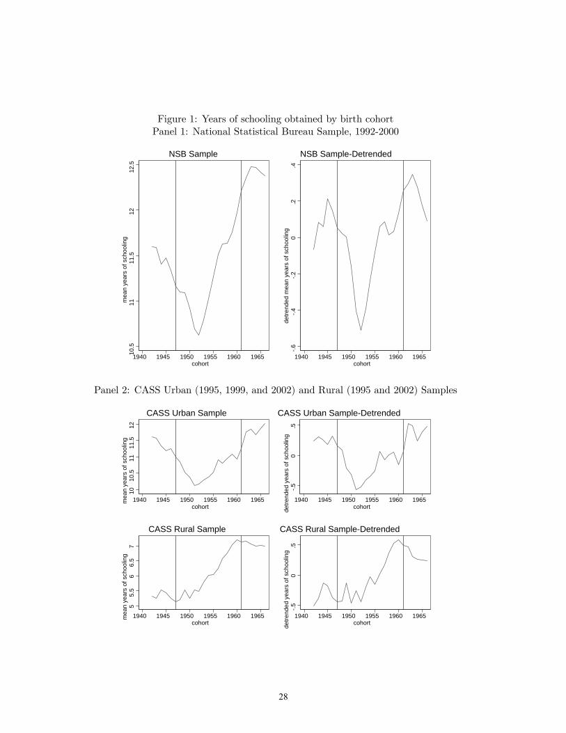
Figure 1: Years of schooling obtained by birth cohortPanel 1: National Statistical Bureau Sample, 1992-2000

10.5

1111

.512

12.5

mea

n ye

ars

of s

choo

ling

1940 1945 1950 1955 1960 1965cohort

NSB Sample

-.6-.4

-.20

.2.4

detre

nded

mea

n ye

ars

of s

choo

ling

1940 1945 1950 1955 1960 1965cohort

NSB Sample-Detrended

Panel 2: CASS Urban (1995, 1999, and 2002) and Rural (1995 and 2002) Samples

1010

.511

11.5

12m

ean

year

s of

sch

oolin

g

1940 1945 1950 1955 1960 1965cohort

CASS Urban Sample

-.50

.5de

trend

ed y

ears

of s

choo

ling

1940 1945 1950 1955 1960 1965cohort

CASS Urban Sample-Detrended

55.

56

6.5

7m

ean

year

s of

sch

oolin

g

1940 1945 1950 1955 1960 1965cohort

CASS Rural Sample

-.50

.5de

trend

ed y

ears

of s

choo

ling

1940 1945 1950 1955 1960 1965cohort

CASS Rural Sample-Detrended

28

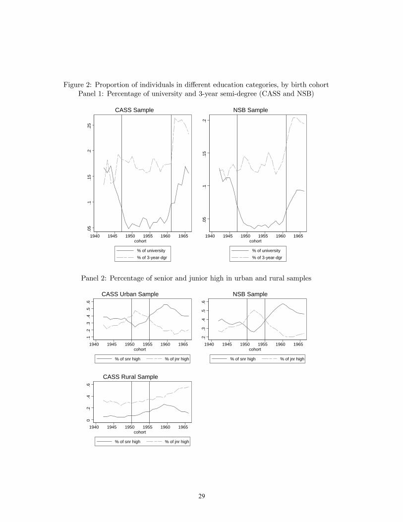
Figure 2: Proportion of individuals in different education categories, by birth cohortPanel 1: Percentage of university and 3-year semi-degree (CASS and NSB)

.05

.1.1

5.2

.25

1940 1945 1950 1955 1960 1965cohort

% of university% of 3-year-dgr

CASS Sample

.05

.1.1

5.2

1940 1945 1950 1955 1960 1965cohort

% of university% of 3-year-dgr

NSB Sample

Panel 2: Percentage of senior and junior high in urban and rural samples

.1.2

.3.4

.5.6

1940 1945 1950 1955 1960 1965cohort

% of snr high % of jnr high

CASS Urban Sample

.2.3

.4.5

.6

1940 1945 1950 1955 1960 1965cohort

% of snr high % of jnr high

NSB Sample

0.2

.4.6

1940 1945 1950 1955 1960 1965cohort

% of snr high % of jnr high

CASS Rural Sample

29

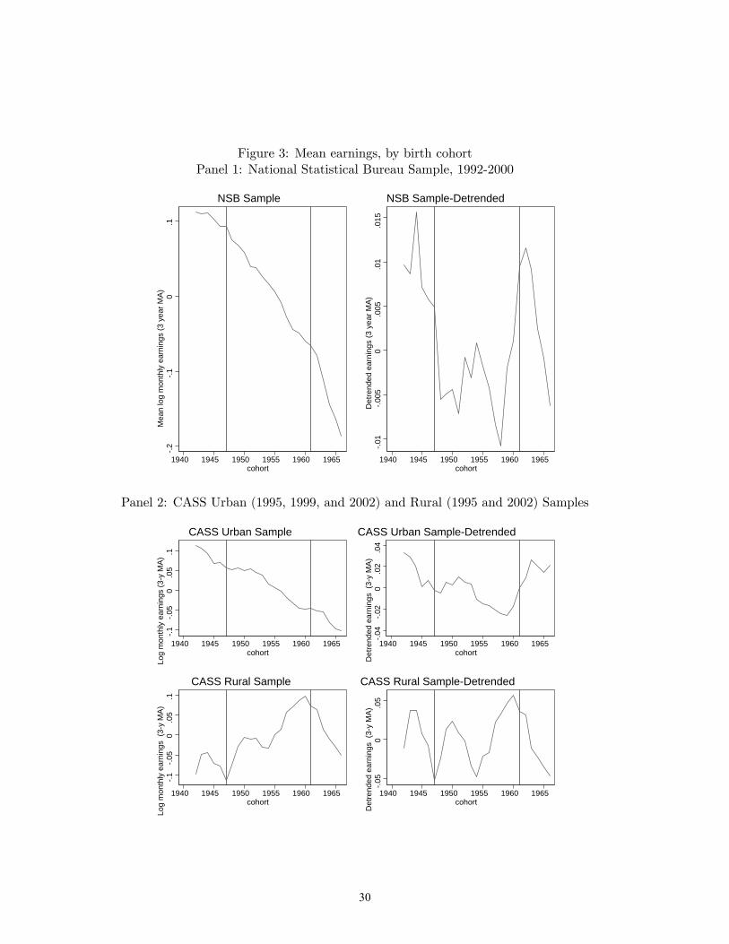
Figure 3: Mean earnings, by birth cohortPanel 1: National Statistical Bureau Sample, 1992-2000

-.2-.1

0.1

Mea

n lo

g m

onth

ly e

arni

ngs

(3 y

ear M

A)

1940 1945 1950 1955 1960 1965cohort

NSB Sample

-.01

-.005

0.0

05.0

1.0

15D

etre

nded

ear

ning

s (3

yea

r MA)

1940 1945 1950 1955 1960 1965cohort

NSB Sample-Detrended

Panel 2: CASS Urban (1995, 1999, and 2002) and Rural (1995 and 2002) Samples

-.1-.0

50

.05

.1Lo

g m

onth

ly e

arni

ngs

(3-y

MA)

1940 1945 1950 1955 1960 1965cohort

CASS Urban Sample

-.04

-.02

0.0

2.0

4D

etre

nded

ear

ning

s (3

-y M

A)

1940 1945 1950 1955 1960 1965cohort

CASS Urban Sample-Detrended

-.1-.0

50

.05

.1Lo

g m

onth

ly e

arni

ngs

(3-y

MA)

1940 1945 1950 1955 1960 1965cohort

CASS Rural Sample

-.05

0.0

5D

etre

nded

ear

ning

s (3

-y M

A)

1940 1945 1950 1955 1960 1965cohort

CASS Rural Sample-Detrended

30

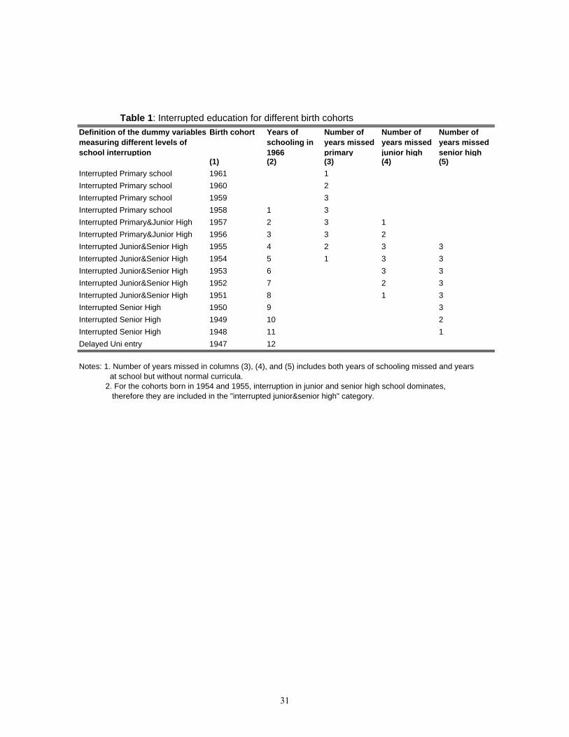
Table 1: Interrupted education for different birth cohorts

(1) (2) (3) (4) (5)Interrupted Primary school 1961 1Interrupted Primary school 1960 2Interrupted Primary school 1959 3Interrupted Primary school 1958 1 3Interrupted Primary&Junior High 1957 2 3 1Interrupted Primary&Junior High 1956 3 3 2Interrupted Junior&Senior High 1955 4 2 3 3Interrupted Junior&Senior High 1954 5 1 3 3Interrupted Junior&Senior High 1953 6 3 3Interrupted Junior&Senior High 1952 7 2 3Interrupted Junior&Senior High 1951 8 1 3Interrupted Senior High 1950 9 3Interrupted Senior High 1949 10 2Interrupted Senior High 1948 11 1Delayed Uni entry 1947 12

Notes: 1. Number of years missed in columns (3), (4), and (5) includes both years of schooling missed and years at school but without normal curricula. 2. For the cohorts born in 1954 and 1955, interruption in junior and senior high school dominates, therefore they are included in the "interrupted junior&senior high" category.

Number of years missed senior high

Years of schooling in 1966

Definition of the dummy variables measuring different levels of school interruption

Birth cohort Number of years missed primary

Number of years missed junior high

31

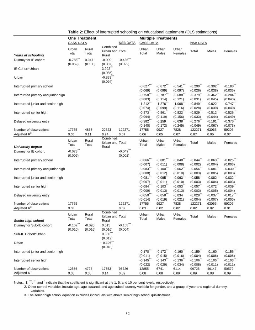
Table 2: Effect of interrupted schooling on educational attainment (OLS estimations)One Treatment Multiple TreatmentsCASS DATA NSB DATA CASS DATA NSB DATA

Years of schooling

Urban Total

Rural Total

Combined Urban and Rural

Total Urban Total

Urban Males

Urban Females Total Males Females

Dummy for IE cohort -0.788*** 0.047 -0.009 -0.436***

(0.059) (0.100) (0.087) (0.022)IE-Cohort*Urban 3.992***

(0.085)Urban -0.833***

(0.094)Interrupted primary school -0.627*** -0.672*** -0.541*** -0.290*** -0.392*** -0.180***

(0.069) (0.099) (0.097) (0.026) (0.038) (0.035)Interrupted primary and junior high -0.758*** -0.787*** -0.688*** -0.379*** -0.462*** -0.284***

(0.083) (0.114) (0.121) (0.031) (0.045) (0.043)Interrupted junior and senior high -1.212*** -1.276*** -1.068*** -0.849*** -0.922*** -0.747***

(0.074) (0.099) (0.116) (0.028) (0.039) (0.040)Interrupted senior high -0.873*** -0.861*** -0.822*** -0.529*** -0.512*** -0.526***

(0.094) (0.119) (0.156) (0.033) (0.044) (0.049)Delayed university entry -0.382*** -0.259 -0.638*** -0.276*** -0.191*** -0.376***

(0.140) (0.172) (0.245) (0.049) (0.067) (0.073)Number of observations 17755 4868 22623 122271 17755 9927 7828 122271 63065 59206Adjusted R2 0.05 0.11 0.24 0.07 0.06 0.05 0.07 0.07 0.05 0.07

University degree

Urban Total

Rural Total

Combined Urban and Rural

Total Urban Total

Urban Males

Urban Females Total Males Females

Dummy for IE cohort -0.073*** -0.049***

(0.006) (0.002)Interrupted primary school -0.066*** -0.081*** -0.048*** -0.044*** -0.063*** -0.025***

(0.007) (0.011) (0.008) (0.002) (0.004) (0.003)Interrupted primary and junior high -0.083*** -0.100*** -0.062*** -0.056*** -0.081*** -0.030***

(0.008) (0.012) (0.010) (0.003) (0.005) (0.003)Interrupted junior and senior high -0.081*** -0.095*** -0.063*** -0.058*** -0.082*** -0.032***

(0.007) (0.011) (0.010) (0.003) (0.004) (0.003)Interrupted senior high -0.084*** -0.103*** -0.053*** -0.057*** -0.072*** -0.039***

(0.009) (0.013) (0.013) (0.003) (0.005) (0.004)Delayed university entry -0.050*** -0.058*** -0.034 -0.028*** -0.037*** -0.017***

(0.014) (0.019) (0.021) (0.004) (0.007) (0.005)Number of observations 17755 122271 17755 9927 7828 122271 63065 59206Adjusted R2 0.03 0.02 0.03 0.02 0.02 0.02 0.02 0.01

Senior high school

Urban Total

Rural Total

Combined Urban and Rural

Total Urban Total

Urban Males

Urban Females Total Males Females

Dummy for Sub-IE cohort -0.167*** -0.020 0.015 -0.153***

(0.010) (0.016) (0.016) (0.004)Sub-IE Cohort*Urban 0.380***

(0.012)Urban -0.196***

(0.018)Interrupted junior and senior high -0.170*** -0.173*** -0.160*** -0.159*** -0.160*** -0.156***

(0.011) (0.015) (0.016) (0.004) (0.006) (0.006)Interrupted senior high -0.145*** -0.143*** -0.136*** -0.106*** -0.105*** -0.103***

(0.022) (0.029) (0.034) (0.008) (0.011) (0.011)Number of observations 12856 4797 17653 96726 12855 6741 6114 96726 46147 50579Adjusted R2 0.08 0.05 0.14 0.09 0.08 0.08 0.09 0.09 0.08 0.09

Notes: 1. ***, **, and * indicate that the coefficient is significant at the 1, 5, and 10 per cent levels, respectively. 2. Other control variables include age, age squared, and age cubed, dummy variable for gender, and a group of year and regional dummy variables. 3. The senior high school equation excludes individuals with above senior high school qualifications.

32

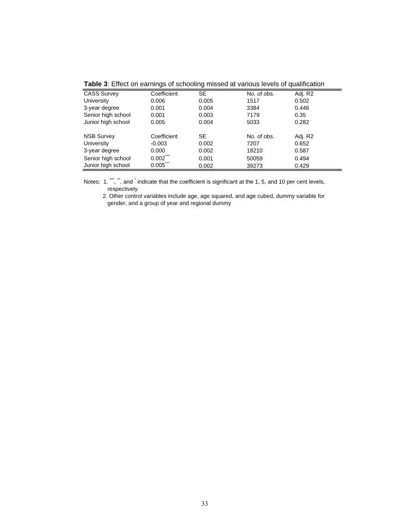
Table 3: Effect on earnings of schooling missed at various levels of qualificationCASS Survey Coefficient SE No. of obs. Adj. R2University 0.006 0.005 1517 0.5023-year degree 0.001 0.004 3384 0.446Senior high school 0.001 0.003 7179 0.35Junior high school 0.005 0.004 5033 0.282

NSB Survey Coefficient SE No. of obs. Adj. R2University -0.003 0.002 7207 0.6523-year degree 0.000 0.002 18210 0.587Senior high school 0.002*** 0.001 50059 0.494Junior high school 0.005*** 0.002 39273 0.429

Notes: 1. ***, **, and * indicate that the coefficient is significant at the 1, 5, and 10 per cent levels, respectively. 2. Other control variables include age, age squared, and age cubed, dummy variable for gender, and a group of year and regional dummy

33

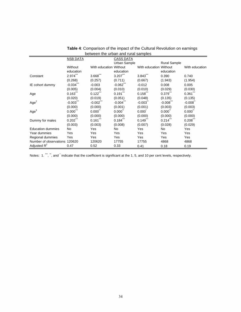
Table 4: Comparison of the impact of the Cultural Revolution on earnings between the urban and rural samples

Without education

With education Without education

With education Without education

With education

Constant 2.974*** 3.668*** 3.207*** 3.843*** 0.390 0.740(0.268) (0.257) (0.711) (0.667) (1.943) (1.954)

IE cohort dummy -0.034*** -0.003 -0.062*** -0.012 0.008 0.005(0.005) (0.004) (0.010) (0.010) (0.029) (0.030)

Age 0.163*** 0.122*** 0.191*** 0.158*** 0.379*** 0.361***

(0.020) (0.019) (0.051) (0.048) (0.135) (0.135)Age2 -0.003*** -0.002*** -0.004*** -0.003** -0.008*** -0.008**

(0.000) (0.000) (0.001) (0.001) (0.003) (0.003)Age3 0.000*** 0.000** 0.000** 0.000* 0.000** 0.000**

(0.000) (0.000) (0.000) (0.000) (0.000) (0.000)Dummy for males 0.202*** 0.161*** 0.184*** 0.149*** 0.214*** 0.208***

(0.003) (0.003) (0.008) (0.007) (0.028) (0.029)Education dummies No Yes No Yes No YesYear dummies Yes Yes Yes Yes Yes YesRegional dummies Yes Yes Yes Yes Yes YesNumber of observations 120620 120620 17755 17755 4868 4868Adjusted R2 0.47 0.52 0.33 0.41 0.18 0.19

Notes: 1. ***, **, and * indicate that the coefficient is significant at the 1, 5, and 10 per cent levels, respectively.

NSB DATA CASS DATAUrban Sample Rural Sample

34

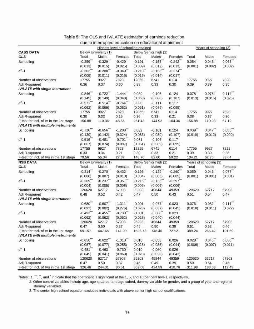
Table 5: The OLS and IV/LATE estimation of earnings reduction due to interrupted education on educational attainment

Highest level of schooling attained Years of schooling (3)CASS DATA Below University (1) Below Senior high (2)OLS Total Males Females Total Males Females Total Males FemalesSchooling -0.359*** -0.329*** -0.429*** -0.191*** -0.155*** -0.242*** 0.054*** 0.048*** 0.063***

(0.013) (0.015) (0.025) (0.009) (0.012) (0.013) (0.001) (0.002) (0.002)eb -1 -0.302*** -0.280*** -0.349*** -0.210*** -0.168*** -0.274***

(0.009) (0.011) (0.016) (0.019) (0.014) (0.017)Number of observations 17755 9927 7828 12855 6741 6114 17755 9927 7828Adj R-squared 0.36 0.37 0.30 0.33 0.33 0.30 0.39 0.39 0.35IV/LATE with single instrumentSchooling -0.846*** -0.722*** -1.444*** 0.030 -0.105 0.124 0.078*** 0.078*** 0.114***

(0.145) (0.149) (0.348) (0.063) (0.080) (0.107) (0.013) (0.015) (0.025)eb -1 -0.571*** -0.514*** -0.764*** 0.030 -0.111 0.117

(0.062) (0.069) (0.082) (0.061) (0.089) (0.095)Number of observations 17755 9927 7828 12855 6741 6114 17755 9927 7828Adj R-squared 0.30 0.32 0.15 0.30 0.33 0.21 0.38 0.37 0.30F-test for incl. of IV in the 1st stage 156.88 110.36 48.56 261.43 144.92 104.36 156.88 110.03 57.19IV/LATE with multiple instrumentsSchooling -0.726*** -0.656*** -1.208*** 0.032 -0.101 0.124 0.039*** 0.047*** 0.056***

(0.139) (0.142) (0.324) (0.063) (0.080) (0.107) (0.010) (0.012) (0.020)eb -1 -0.516*** -0.481*** -0.701*** 0.031 -0.106 0.117

(0.067) (0.074) (0.097) (0.061) (0.089) (0.095)Number of observations 17755 9927 7828 12855 6741 6114 17755 9927 7828Adj R-squared 0.33 0.34 0.21 0.30 0.33 0.21 0.39 0.39 0.35F-test for incl. of IVs in the 1st stage 79.56 55.34 22.32 148.76 82.60 59.22 104.21 62.76 33.04NSB DATA Below University (1) Below Senior high (2) Years of schooling (3)OLS Total Males Females Total Males Females Total Males FemalesSchooling -0.314*** -0.270*** -0.432*** -0.195*** -0.129*** -0.260*** 0.059*** 0.046*** 0.077***

(0.006) (0.007) (0.013) (0.004) (0.005) (0.005) (0.001) (0.001) (0.001)eb -1 -0.269*** -0.237*** -0.351*** -0.215*** -0.138*** -0.297***

(0.004) (0.005) (0.008) (0.005) (0.006) (0.006)Number of observations 120620 62717 57903 95203 45844 49359 120620 62717 57903Adj R-squared 0.48 0.52 0.42 0.47 0.50 0.43 0.51 0.54 0.47IV/LATE with single instrumentSchooling -0.680*** -0.607*** -1.311*** -0.001 -0.077** 0.023 0.076*** 0.082*** 0.111***

(0.092) (0.082) (0.276) (0.028) (0.037) (0.045) (0.010) (0.011) (0.022)eb -1 -0.493*** -0.455*** -0.730*** -0.001 -0.080** 0.023

(0.062) (0.062) (0.062) (0.028) (0.040) (0.044)Number of observations 120620 62717 57903 95203 45844 49359 120620 62717 57903Adj R-squared 0.47 0.50 0.37 0.45 0.50 0.39 0.51 0.52 0.46F-test for incl. of IV in the 1st stage 591.57 447.65 141.09 1523.72 748.46 727.21 389.24 265.42 101.69IV/LATE with multiple instrumentsSchooling -0.656*** -0.622*** -1.310*** 0.010 -0.058 0.026 0.028*** 0.045*** 0.030***

(0.087) (0.077) (0.255) (0.028) (0.036) (0.044) (0.006) (0.007) (0.011)eb -1 -0.481*** -0.463*** -0.730*** 0.010 -0.060 0.026

(0.045) (0.041) (0.069) (0.028) (0.038) (0.043)Number of observations 120620 62717 57903 95203 45844 49359 120620 62717 57903Adj R-squared 0.47 0.50 0.37 0.45 0.49 0.39 0.50 0.54 0.45F-test for incl. of IVs in the 1st stage 326.46 244.31 80.51 862.08 424.59 410.76 311.98 188.53 112.49

Notes: 1. ***, **, and * indicate that the coefficient is significant at the 1, 5, and 10 per cent levels, respectively. 2. Other control variables include age, age squared, and age cubed, dummy variable for gender, and a group of year and regional dummy variables. 3. The senior high school equation excludes individuals with above senior high school qualifications.

35

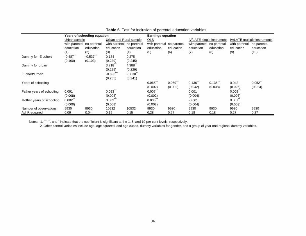
Table 6: Test for inclusion of parental education variablesYears of schooling equation Earnings equationUrban sample Urban and Rural sample OLS IV/LATE single instrument IV/LATE multiple instrumentswith parental education

no parental education

with parental education

no parental education

with parental education

no parental education

with parental education

no parental education

with parental education

no parental education

(1) (2) (3) (4) (5) (6) (7) (8) (9) (10)Dummy for IE cohort -0.487*** -0.537*** 0.184 0.275

(0.100) (0.103) (0.239) (0.245)Dummy for urban 3.718*** 4.388***

(0.225) (0.229)IE chort*Urban -0.696*** -0.838***

(0.235) (0.241)Years of schooling 0.065*** 0.069*** 0.136*** 0.135*** 0.042 0.052**

(0.002) (0.002) (0.042) (0.038) (0.026) (0.024)Father years of schooling 0.091*** 0.093*** 0.007*** 0.001 0.009***

(0.008) (0.008) (0.002) (0.004) (0.003)Mother years of schooling 0.082*** 0.082*** 0.005*** -0.001 0.007**

(0.008) (0.008) (0.002) (0.004) (0.003)Number of observations 9930 9930 10532 10532 9930 9930 9930 9930 9930 9930Adj R-squared 0.09 0.04 0.19 0.15 0.28 0.27 0.18 0.18 0.27 0.27

Notes: 1. ***, **, and * indicate that the coefficient is significant at the 1, 5, and 10 per cent levels, respectively. 2. Other control variables include age, age squared, and age cubed, dummy variables for gender, and a group of year and regional dummy variables.

36

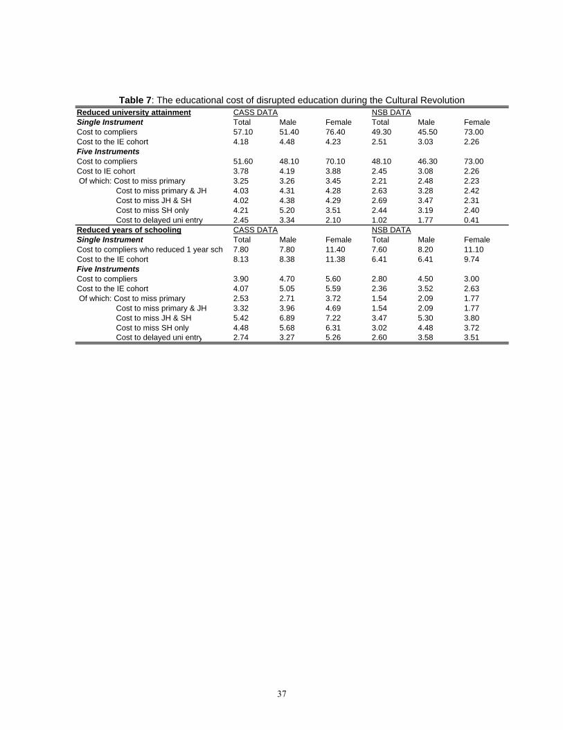
Reduced university attainment CASS DATA NSB DATASingle Instrument Total Male Female Total Male FemaleCost to compliers 57.10 51.40 76.40 49.30 45.50 73.00Cost to the IE cohort 4.18 4.48 4.23 2.51 3.03 2.26Five InstrumentsCost to compliers 51.60 48.10 70.10 48.10 46.30 73.00Cost to IE cohort 3.78 4.19 3.88 2.45 3.08 2.26 Of which: Cost to miss primary 3.25 3.26 3.45 2.21 2.48 2.23 Cost to miss primary & JH 4.03 4.31 4.28 2.63 3.28 2.42 Cost to miss JH & SH 4.02 4.38 4.29 2.69 3.47 2.31 Cost to miss SH only 4.21 5.20 3.51 2.44 3.19 2.40 Cost to delayed uni entry 2.45 3.34 2.10 1.02 1.77 0.41Reduced years of schooling CASS DATA NSB DATASingle Instrument Total Male Female Total Male FemaleCost to compliers who reduced 1 year sch 7.80 7.80 11.40 7.60 8.20 11.10Cost to the IE cohort 8.13 8.38 11.38 6.41 6.41 9.74Five InstrumentsCost to compliers 3.90 4.70 5.60 2.80 4.50 3.00Cost to the IE cohort 4.07 5.05 5.59 2.36 3.52 2.63 Of which: Cost to miss primary 2.53 2.71 3.72 1.54 2.09 1.77 Cost to miss primary & JH 3.32 3.96 4.69 1.54 2.09 1.77 Cost to miss JH & SH 5.42 6.89 7.22 3.47 5.30 3.80 Cost to miss SH only 4.48 5.68 6.31 3.02 4.48 3.72 Cost to delayed uni entry 2.74 3.27 5.26 2.60 3.58 3.51

Table 7: The educational cost of disrupted education during the Cultural Revolution

37

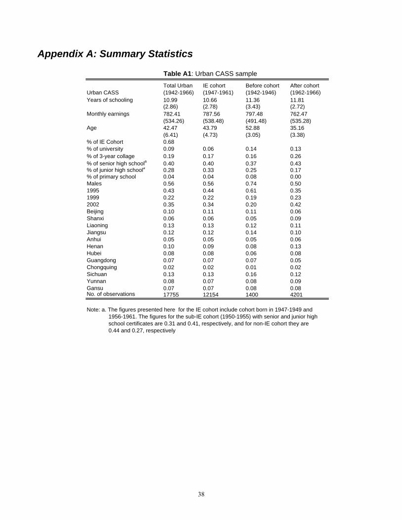
Appendix A: Summary Statistics

Table A1: Urban CASS sample

Urban CASSTotal Urban (1942-1966)

IE cohort (1947-1961)

Before cohort (1942-1946)

After cohort (1962-1966)

Years of schooling 10.99 10.66 11.36 11.81(2.86) (2.78) (3.43) (2.72)

Monthly earnings 782.41 787.56 797.48 762.47(534.26) (538.48) (491.48) (535.28)

Age 42.47 43.79 52.88 35.16(6.41) (4.73) (3.05) (3.38)

% of IE Cohort 0.68% of university 0.09 0.06 0.14 0.13% of 3-year collage 0.19 0.17 0.16 0.26% of senior high schoola 0.40 0.40 0.37 0.43% of junior high schoola 0.28 0.33 0.25 0.17% of primary school 0.04 0.04 0.08 0.00Males 0.56 0.56 0.74 0.501995 0.43 0.44 0.61 0.351999 0.22 0.22 0.19 0.232002 0.35 0.34 0.20 0.42Beijing 0.10 0.11 0.11 0.06Shanxi 0.06 0.06 0.05 0.09Liaoning 0.13 0.13 0.12 0.11Jiangsu 0.12 0.12 0.14 0.10Anhui 0.05 0.05 0.05 0.06Henan 0.10 0.09 0.08 0.13Hubei 0.08 0.08 0.06 0.08Guangdong 0.07 0.07 0.07 0.05Chongquing 0.02 0.02 0.01 0.02Sichuan 0.13 0.13 0.16 0.12Yunnan 0.08 0.07 0.08 0.09Gansu 0.07 0.07 0.08 0.08No. of observations 17755 12154 1400 4201

Note: a. The figures presented here for the IE cohort include cohort born in 1947-1949 and 1956-1961. The figures for the sub-IE cohort (1950-1955) with senior and junior high school certificates are 0.31 and 0.41, respectively, and for non-IE cohort they are 0.44 and 0.27, respectively

38

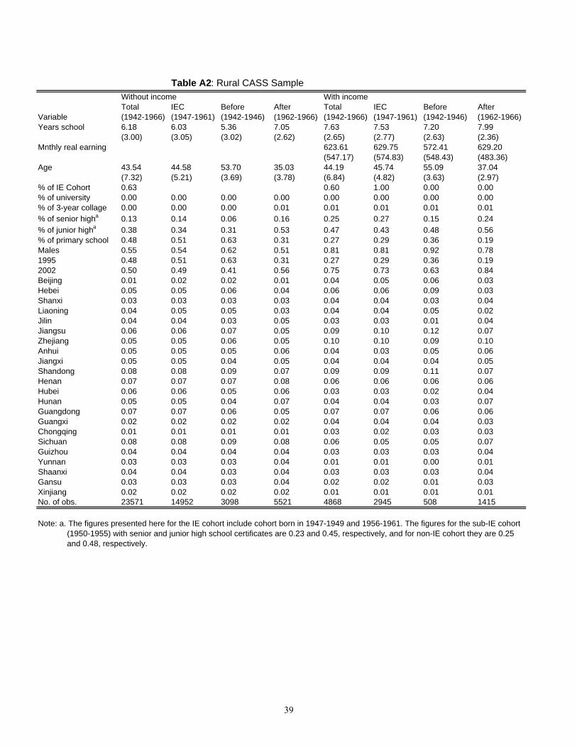
Table A2: Rural CASS Sample

Total IEC Before After Total IEC Before AfterVariable (1942-1966) (1947-1961) (1942-1946) (1962-1966) (1942-1966) (1947-1961) (1942-1946) (1962-1966)Years school 6.18 6.03 5.36 7.05 7.63 7.53 7.20 7.99

(3.00) (3.05) (3.02) (2.62) (2.65) (2.77) (2.63) (2.36)Mnthly real earning 623.61 629.75 572.41 629.20

(547.17) (574.83) (548.43) (483.36)Age 43.54 44.58 53.70 35.03 44.19 45.74 55.09 37.04

(7.32) (5.21) (3.69) (3.78) (6.84) (4.82) (3.63) (2.97)% of IE Cohort 0.63 0.60 1.00 0.00 0.00% of university 0.00 0.00 0.00 0.00 0.00 0.00 0.00 0.00% of 3-year collage 0.00 0.00 0.00 0.01 0.01 0.01 0.01 0.01% of senior higha 0.13 0.14 0.06 0.16 0.25 0.27 0.15 0.24% of junior higha 0.38 0.34 0.31 0.53 0.47 0.43 0.48 0.56% of primary school 0.48 0.51 0.63 0.31 0.27 0.29 0.36 0.19Males 0.55 0.54 0.62 0.51 0.81 0.81 0.92 0.781995 0.48 0.51 0.63 0.31 0.27 0.29 0.36 0.192002 0.50 0.49 0.41 0.56 0.75 0.73 0.63 0.84Beijing 0.01 0.02 0.02 0.01 0.04 0.05 0.06 0.03Hebei 0.05 0.05 0.06 0.04 0.06 0.06 0.09 0.03Shanxi 0.03 0.03 0.03 0.03 0.04 0.04 0.03 0.04Liaoning 0.04 0.05 0.05 0.03 0.04 0.04 0.05 0.02Jilin 0.04 0.04 0.03 0.05 0.03 0.03 0.01 0.04Jiangsu 0.06 0.06 0.07 0.05 0.09 0.10 0.12 0.07Zhejiang 0.05 0.05 0.06 0.05 0.10 0.10 0.09 0.10Anhui 0.05 0.05 0.05 0.06 0.04 0.03 0.05 0.06Jiangxi 0.05 0.05 0.04 0.05 0.04 0.04 0.04 0.05Shandong 0.08 0.08 0.09 0.07 0.09 0.09 0.11 0.07Henan 0.07 0.07 0.07 0.08 0.06 0.06 0.06 0.06Hubei 0.06 0.06 0.05 0.06 0.03 0.03 0.02 0.04Hunan 0.05 0.05 0.04 0.07 0.04 0.04 0.03 0.07Guangdong 0.07 0.07 0.06 0.05 0.07 0.07 0.06 0.06Guangxi 0.02 0.02 0.02 0.02 0.04 0.04 0.04 0.03Chongqing 0.01 0.01 0.01 0.01 0.03 0.02 0.03 0.03Sichuan 0.08 0.08 0.09 0.08 0.06 0.05 0.05 0.07Guizhou 0.04 0.04 0.04 0.04 0.03 0.03 0.03 0.04Yunnan 0.03 0.03 0.03 0.04 0.01 0.01 0.00 0.01Shaanxi 0.04 0.04 0.03 0.04 0.03 0.03 0.03 0.04Gansu 0.03 0.03 0.03 0.04 0.02 0.02 0.01 0.03Xinjiang 0.02 0.02 0.02 0.02 0.01 0.01 0.01 0.01No. of obs. 23571 14952 3098 5521 4868 2945 508 1415

Note: a. The figures presented here for the IE cohort include cohort born in 1947-1949 and 1956-1961. The figures for the sub-IE cohort (1950-1955) with senior and junior high school certificates are 0.23 and 0.45, respectively, and for non-IE cohort they are 0.25 and 0.48, respectively.

Without income With income

39

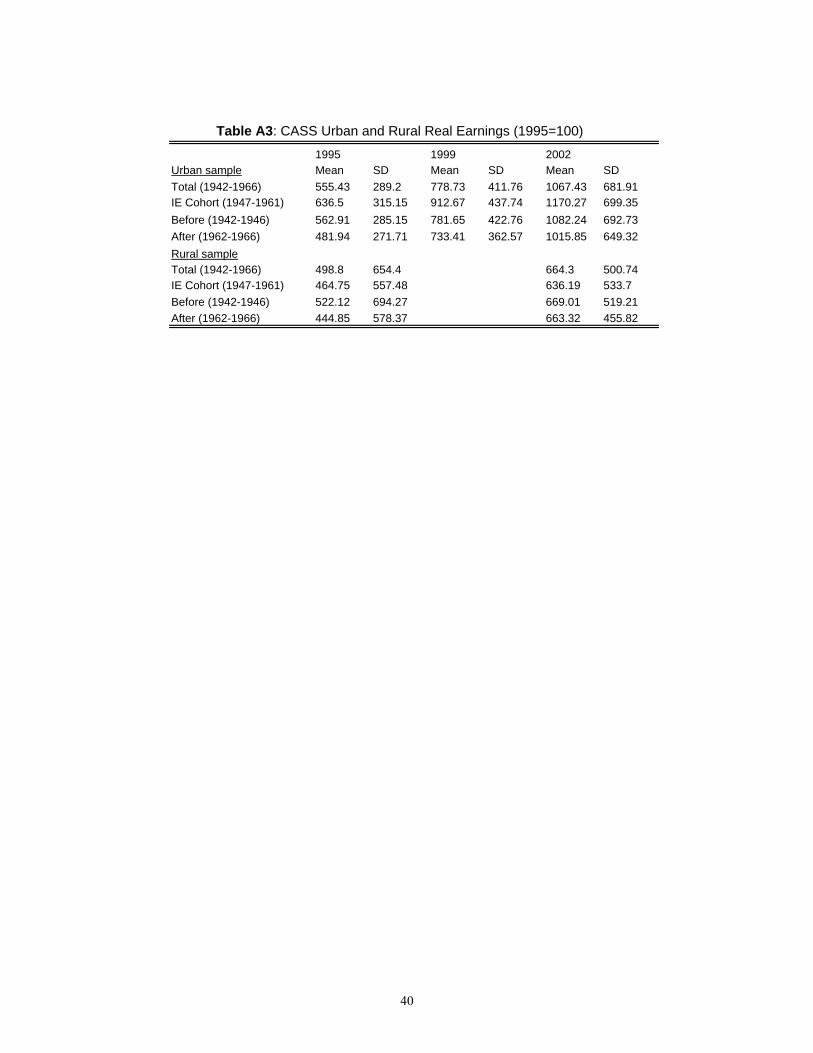
Table A3: CASS Urban and Rural Real Earnings (1995=100)

Urban sample Mean SD Mean SD Mean SDTotal (1942-1966) 555.43 289.2 778.73 411.76 1067.43 681.91IE Cohort (1947-1961) 636.5 315.15 912.67 437.74 1170.27 699.35Before (1942-1946) 562.91 285.15 781.65 422.76 1082.24 692.73After (1962-1966) 481.94 271.71 733.41 362.57 1015.85 649.32Rural sampleTotal (1942-1966) 498.8 654.4 664.3 500.74IE Cohort (1947-1961) 464.75 557.48 636.19 533.7Before (1942-1946) 522.12 694.27 669.01 519.21After (1962-1966) 444.85 578.37 663.32 455.82

1995 1999 2002

40

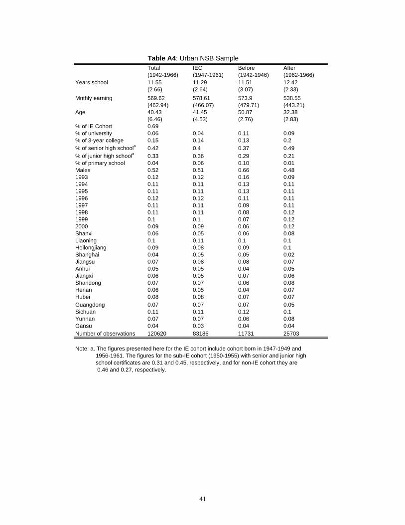
Table A4: Urban NSB SampleTotal IEC Before After(1942-1966) (1947-1961) (1942-1946) (1962-1966)

Years school 11.55 11.29 11.51 12.42(2.66) (2.64) (3.07) (2.33)

Mnthly earning 569.62 578.61 573.9 538.55(462.94) (466.07) (479.71) (443.21)

Age 40.43 41.45 50.87 32.38(6.46) (4.53) (2.76) (2.83)

% of IE Cohort 0.69% of university 0.06 0.04 0.11 0.09% of 3-year college 0.15 0.14 0.13 0.2% of senior high schoola 0.42 0.4 0.37 0.49% of junior high schoola 0.33 0.36 0.29 0.21% of primary school 0.04 0.06 0.10 0.01Males 0.52 0.51 0.66 0.481993 0.12 0.12 0.16 0.091994 0.11 0.11 0.13 0.111995 0.11 0.11 0.13 0.111996 0.12 0.12 0.11 0.111997 0.11 0.11 0.09 0.111998 0.11 0.11 0.08 0.121999 0.1 0.1 0.07 0.122000 0.09 0.09 0.06 0.12Shanxi 0.06 0.05 0.06 0.08Liaoning 0.1 0.11 0.1 0.1Heilongjiang 0.09 0.08 0.09 0.1Shanghai 0.04 0.05 0.05 0.02Jiangsu 0.07 0.08 0.08 0.07Anhui 0.05 0.05 0.04 0.05Jiangxi 0.06 0.05 0.07 0.06Shandong 0.07 0.07 0.06 0.08Henan 0.06 0.05 0.04 0.07Hubei 0.08 0.08 0.07 0.07Guangdong 0.07 0.07 0.07 0.05Sichuan 0.11 0.11 0.12 0.1Yunnan 0.07 0.07 0.06 0.08Gansu 0.04 0.03 0.04 0.04Number of observations 120620 83186 11731 25703

Note: a. The figures presented here for the IE cohort include cohort born in 1947-1949 and 1956-1961. The figures for the sub-IE cohort (1950-1955) with senior and junior high school certificates are 0.31 and 0.45, respectively, and for non-IE cohort they are 0.46 and 0.27, respectively.

41

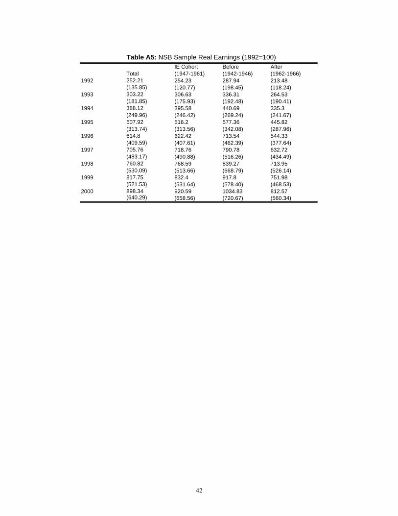
Table A5: NSB Sample Real Earnings (1992=100)IE Cohort Before After(1947-1961) (1942-1946) (1962-1966)

1992 252.21 254.23 287.94 213.48(135.85) (120.77) (198.45) (118.24)

1993 303.22 306.63 336.31 264.53(181.85) (175.93) (192.48) (190.41)

1994 388.12 395.58 440.69 335.3(249.96) (246.42) (269.24) (241.67)

1995 507.92 516.2 577.36 445.82(313.74) (313.56) (342.08) (287.96)

1996 614.8 622.42 713.54 544.33(409.59) (407.61) (462.39) (377.64)

1997 705.76 718.76 790.78 632.72(483.17) (490.88) (516.26) (434.49)

1998 760.82 768.59 839.27 713.95(530.09) (513.66) (668.79) (526.14)

1999 817.75 832.4 917.8 751.98(521.53) (531.64) (578.40) (468.53)

2000 898.34 920.59 1034.83 812.57(640.29) (658.56) (720.67) (560.34)

Total

42