Exploring the Contribution of Temporary and Permanent ... · Exploring the Contribution of...
30
Working Paper Exploring the Contribution of Temporary and Permanent Shocks to the Real Effective Exchange Rate on the Current Account Imbalance in Jamaica Tamalia Franklin 1 International Economics Department Research and Economic Programming Division Bank of Jamaica August 2010 Abstract This paper reviews the relationship between the real effective exchange rate (REER) and current account imbalances, with a view to determining the proportion of the Jamaican current account imbalance that can be corrected with a REER adjustment. Most studies have failed to identify a positive and significant relationship between the REER and the Jamaican current account. This study contends that this may reflect the differing sources of shocks to the variables. Using the Blanchard and Quah (1989) methodology, results indicate that temporary shocks have a larger role in explaining the variation in the REER, while permanent shocks play a larger role in the explanation of the Jamaican current account. Variance decomposition results indicate that only a negligible portion of the current account imbalance could be corrected through a REER depreciation. In this regard, achieving a sustainable current account balance requires a positive permanent (productivity) shock. Keywords: Real effective exchange rate, structural shocks, SVAR JEL Classification codes: F12, F32, F41 1 The views expressed are those of the author and do not necessarily reflect those of the Bank of Jamaica. [1]
Transcript of Exploring the Contribution of Temporary and Permanent ... · Exploring the Contribution of...

Working Paper
Exploring the Contribution of Temporary and Permanent Shocks to the
Real Effective Exchange Rate on the Current Account Imbalance in Jamaica
Tamalia Franklin1
International Economics Department Research and Economic Programming Division
Bank of Jamaica
August 2010
Abstract This paper reviews the relationship between the real effective exchange rate (REER) and current account imbalances, with a view to determining the proportion of the Jamaican current account imbalance that can be corrected with a REER adjustment. Most studies have failed to identify a positive and significant relationship between the REER and the Jamaican current account. This study contends that this may reflect the differing sources of shocks to the variables. Using the Blanchard and Quah (1989) methodology, results indicate that temporary shocks have a larger role in explaining the variation in the REER, while permanent shocks play a larger role in the explanation of the Jamaican current account. Variance decomposition results indicate that only a negligible portion of the current account imbalance could be corrected through a REER depreciation. In this regard, achieving a sustainable current account balance requires a positive permanent (productivity) shock.
Keywords: Real effective exchange rate, structural shocks, SVAR
JEL Classification codes: F12, F32, F41
1 The views expressed are those of the author and do not necessarily reflect those of the Bank of Jamaica.
[1]
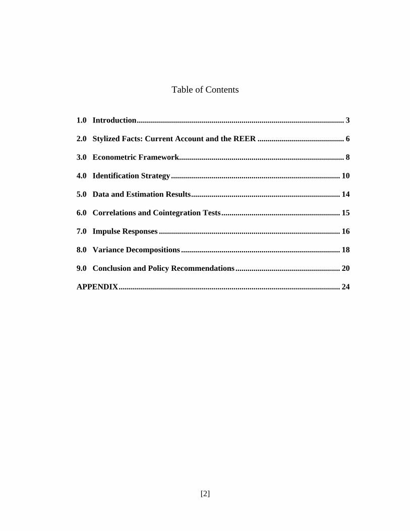
Table of Contents
1.0 Introduction....................................................................................................... 3
2.0 Stylized Facts: Current Account and the REER ........................................... 6
3.0 Econometric Framework.................................................................................. 8
4.0 Identification Strategy .................................................................................... 10
5.0 Data and Estimation Results.......................................................................... 14
6.0 Correlations and Cointegration Tests........................................................... 15
7.0 Impulse Responses .......................................................................................... 16
8.0 Variance Decompositions ............................................................................... 18
9.0 Conclusion and Policy Recommendations .................................................... 20
APPENDIX.............................................................................................................. 24
[2]

1.0 Introduction While the role of real exchange rates in the determination of current account balances
constitutes an essential component of the theoretical framework of both traditional and
modern approaches to international macroeconomics, very limited empirical evidence has
been produced that explicitly focuses on this relationship. This, according to Stockman
(1978), may be attributed to the fact that most studies that try to link the real effective
exchange rate (REER) to the current account usually find anomalous results. He noted
that this may reflect the fact that flexible exchange rates have exhibited significant
volatility and its relationship with prices has deviated from the purchasing power parity
(PPP) theory. He further contends that changes in the exchange rate have also failed to
resemble contemporaneous changes in relative price levels in either magnitude or
direction. Against this background, much research has been centred on understanding the
determinants of the REER and the current account in an effort to determine the reasons
behind anomalous results being obtained..
According to the Mundell-Fleming model, an appreciation in the REER and hence a
decline in a country’s competitiveness position, leads to a worsening trade balance or
“external imbalance” and, ultimately a worsening current account balance (Kwalingana et
al., 2009). It therefore holds that a depreciation of the REER should restore balance or
equilibrium given that the Marshall-Lerner condition holds.2 This REER depreciation can
be achieved either by a depreciation of the trade-weighted exchange rate (obtained
through a depreciation of the nominal exchange rate) or by a decline in relative inflation.
Similar to results from Stockman (1978), Lee and Chinn (2002) argued that much
empirical evidence to support this relationship between the current account and the REER
has failed to be forthcoming. This, they attributed to the differing sources of shocks that
drive the REER and the current account. Rogers (1998) and Lee and Chinn (2005),
contend that temporary shocks are synonymous with monetary shocks, while permanent
shocks are largely interpreted as productivity shocks. In this context, the role of monetary
2 The Marshall-Lerner condition states that for a currency devaluation to have a positive impact on the trade balance, the sum of price elasticity of exports and imports (in absolute values), must be greater than 1. If exported goods are elastic to price, their quantity demanded will be proportionately more than the decrease in price, and total export revenue will increase. Similarly, if the goods imported are price elastic, then total import expenditure will decrease. Both will then improve the trade balance.
[3]

adjustments and changes in output, play a role in the determination of the exchange rate
and the current account and consequently their anticipated relationship. As a result, it is
expected that a correction in the current imbalance may be facilitated by a REER
adjustment given that both variables are largely driven by similar shocks.
Conventional theory holds that the transmission mechanism from changes in the REER to
an adjustment in the current account includes a real depreciation of the domestic
currency. This is generally seen as leading to a less-than-proportionate increase in the
prices of exports which are measured in domestic currency, which means that export
prices would fall when measured in terms of the foreign currency, thus making exports
more competitive. The net effect is an increase in the volume of exports. Similarly, a real
depreciation in the exchange rate causes the price of imports measured in the domestic
currency to rise, thus reducing demand for these goods and lowering import volumes. As
long as the volume responses of imports and exports to the relative price shifts are
sufficiently large to outweigh the negative terms-of-trade shift that arises because export
prices rise less than import prices, the trade balance and hence the current account
balance will improve. It must be noted that this approach assumes that the inflationary
process induced by the lower exchange rate does not act to completely offset the initial
change in relative prices thus facilitating a real depreciation.
Lee and Chinn (2002) concluded that most of the movements in the real exchange rate in
G-7 countries were related to permanent shocks whose effect on the current account was
negligible or in the opposite direction to the temporary shocks. They later decomposed
the current account balances of the three largest economies (US, Japan and the Euro
Area) to determine how much of the current account balance was attributable to either
temporary or permanent shocks. They determined that in 2003 and 2004, nearly two per
cent of the US current account deficit as a percentage of GDP was found to be influenced
by temporary shocks. As a result, a correction of that amount of the current account
deficit would go hand in hand with depreciation in the US real exchange rate. For Japan
and the Euro area, however, a small portion of their current account surpluses were
driven by temporary shocks, which would be accompanied by an appreciation in the
[4]
respective currencies. Notably, Gauthier and Tessier (2002) also determined that a
permanent shock induced an improvement in the current account balance, coupled with
an appreciation of the real exchange rate. Therefore, the expected relationship as posited
by the Mundell-Fleming model was not fully observed.
McDonald (1998) explored four different approaches to analyzing the importance of
temporary shocks relative to permanent shocks in driving changes in the exchange rate by
incorporating the Blanchard and Quah (1989) identification methods. He determined that
the systematic component of the real exchange rate was related to permanent factors such
as productivity, net foreign asset accumulation, national savings imbalances and terms of
trade effects. Cavallari (1999) analyzed the effect of both temporary and permanent
shocks on the current account across G-7 countries where it was determined that in
general, at very short horizons, current account fluctuations were largely attributed to
temporary shocks while permanent shocks were increasingly found to affect the variance
of the current account in the longer horizons, particularly after a year. In particular,
results from the UK, Italy, France and Canada indicated that a negative temporary shock
caused the current account to go into surplus while in the US, Germany and Japan, the
current account initially deteriorated and slowly improved, albeit not always
significantly. Zhang (2009) later illustrated that temporary shocks accounted for a
substantial fraction of the terms of trade fluctuations and were also quantitatively
important for the real exchange rate movements. Contrary to Cavallari (1999), there was
no evidence showing that temporary shocks played any significant role in the current
account fluctuations of major economies except for those that were seen in Japan,
Germany, and the US.
In the context of the foregoing, it is evident that mixed results have been obtained in
relation to the source of shocks to the REER and the current account and the effect of
these shocks on their expected relationship. The aim of this paper is to therefore
determine the extent to which temporary and permanent shocks have influenced these
variables in the Jamaican context and, based on the results, a better understanding of their
relationship may be garnered. This will be done by utilizing a variation of the Blanchard
[5]

and Quah (1989) model to determine which shocks largely influence each variable.
Results from correlation and cointegration tests suggest that the REER has been largely
driven by temporary shocks while the current account has been largely influenced by
permanent shocks. Indeed approximately 1.0 per cent of the portion of the current
account imbalance attributed to temporary shocks could be corrected by depreciation in
the real exchange rate that is also caused by a temporary shock.
2.0 Stylized Facts: Current Account and the REER Over the past decade, Jamaica has consistently run a current account deficit along with
significant depreciations in the exchange rate relative to our major trading partners. This
has not only been observed in developing economies such as Jamaica and Mexico but
also in advanced economies such as the USA and the UK (see Figures 1a and 1b,
Appendix). For Jamaica, the current account deficit has been largely driven by persistent
merchandise trade deficits. The resulting negative trade balance has largely reflected the
country’s dependency on imports (see Figure 2, Appendix). Data over the period, April
1995 to December 2009, indicate that Raw Material imports accounted for 41.1 per cent
of total imports, followed closely by consumer goods and capital goods imports which
accounted for 39.8 per cent and 19.2 per cent of total imports, respectively. The major
source of export earnings have emanated from the major traditional export crops of sugar,
bauxite and alumina. Over the review period, this has constituted approximately 65.2 per
cent of total exports, of which alumina earnings comprised 51.9 per cent.
In general, the current account deficit as a percentage of GDP has displayed an upward
trend (see Figure 3, Appendix).3 For the first five years of the sample period (1996 to
2000) the current account deficit averaged 3.2 per cent of GDP compared to an average
of 12.4 per cent from 2005 to 2009. This largely reflected the widening trade deficit
during the period. The years 2008 and 2009 represented the highest trade deficit to be
recorded in the economy where imports exceeded exports by 275.0 per cent and 333.8 per
cent, respectively. This was in the context of a 42.5 per cent increase in oil prices in 2008
3 The figures represent the absolute values of the current account deficit.
[6]

and a fall off in mining exports due to the closure of three alumina plants in 2009.4
Exports, remained relatively constant during the period, with significant increases of 29.5
per cent, 11.1 per cent and 14.9 per cent only being observed from 2006 to 2008.5 There
was also a complete cessation in banana exports since 2007 due to the termination of
export activities attributed to the impact of hurricanes.
Apart from goods exports, the main source of foreign exchange earnings is services
exports, primarily earnings from tourism. Notably, stop-over tourist arrivals grew at an
average annual rate of approximately 3.0 per cent between 1996 and 2009 while visitor
expenditure increased by an annual average rate of 4.7 per cent. Foreign currency inflows
through remittances, which fall under the Current Transfers sub-account, is another major
earner of foreign currency, which has grown at an annual average rate of 12.7 per cent
over the period and has represented an average of 13.3 per cent of GDP.
In relation to the path of Jamaica’s REER index, Williams (2008) outlined that Jamaica’s
REER index has largely moved in line with macro-economic fundamentals. This was
determined using the Equilibrium Real Exchange Rate (ERER) approach which utilized
multilateral exchange rates (REER), the ratio of Jamaica’s net foreign assets (NFA) to
GDP, the short term interest rate differential, Jamaica’s relative labour productivity, the
terms of trade, trade restrictions measured by implicit tariff price and government
consumption as a ratio to GDP. Despite the relatively stable level of competitiveness
observed over the period there has been significant depreciation in the nominal exchange
rate by approximately 155.7 per cent from end-December 1996 to end-December 2009.
This depreciation in the nominal exchange rate was particularly evident in 2003 and 2008
4 Oil prices averaged US$94.10 per barrel in 2008 compared to a five-year average of US$47.50 during 2003 to 2007. The closure of the alumina plants occurred in the context of low demand stemming from the global economic downturn since 2008. 5 The increase in export earnings in 2006 and 2007 was due to significant increases in alumina prices of 16.8 per cent and 19.3 per cent, respectively, while non-traditional exports increased by over 45.0 per cent during 2008.
[7]

when the weighted average selling rate (WASR) depreciated by 15.9 per cent and 12.2
per cent, respectively.6
In terms of the relationship between the current account and the REER, Figure 4
Appendix, indicates that the two variables moved together over the period. It has been
observed that as the REER index increased (referred to as a REER appreciation); there
was a similar worsening of the current account deficit. According to Henry and
Longmore (2003), the literature does not suggest that the current account adjustment to
changes in the REER must be instantaneous. In a dynamic setting, the improvement on
the current account in a particular year may be associated with depreciation in the REER
in prior periods and the possible exposure of these variables to external shocks. As a
result, it may be difficult to make firm conclusions from Figure 4. This therefore points to
the need for more rigorous empirical work to ascertain the relationship between the two
variables.
3.0 Econometric Framework To understand the trend-cycle movements in macroeconomic variables and the sources of
shocks, univariate measures such as that put forward by Beveridge and Nelson (1981)
indicated that macroeconomic variables could be disaggregated into their stationary and
non-stationary components. These components, they denoted as the temporary and
permanent components, respectively. The temporary component represents the
predictable part of the data, which dissipates with time as the series tends to its permanent
level. The permanent component comprises a random walk with the same rate of drift as
in the original data as well as a disturbance term proportional to that of the original data.
De Silva (2007) utilized the Beveridge-Nelson vector innovation structural time series
6 The depreciation in 2003 was attributed to a decline in market confidence triggered by a confluence of factors, including deterioration of the fiscal and balance of payments accounts, and the related downgrade of the outlook of Jamaica’s sovereign debt by Standard and Poor’s (S&P). This was facilitated by the high level of Jamaica dollar liquidity. Most of the depreciation in 2009 occurred in the first quarter, where the dollar lost J$7.80 (10.0 per cent) which was largely due to a contraction in net private capital inflows. This stemmed from the temporary removal of credit lines in the context of the global economic crisis which started in the December quarter of 2008.
[8]

framework to decompose the GDP of Australia, America and the UK into their temporary
and permanent components. It was shown that this specification was simpler than
conventional state space and cointegration approaches while also showing how to model
inter-series dependencies between the variables. However, the univariate approaches of
decomposition have been criticized by Nelson (2006) who determined that the widely
used univariate trend-cycle decompositions employed in macro-econometric analysis
were ineffective in predicting economic activity in real time. He added that only the
modest momentum growth captured by the Beveridge-Nelson cycle estimates, account
for some level of predictability. As a result, the bivariate approach such as that proposed
by Blanchard and Quah (1989) had the advantage over the Beveridge-Nelson
decomposition by giving a unique decomposition for the series in question and making
use of the additional information contained in the other variable (Erlat and Erlat, 1998).
Consistent with the findings by Erlat and Erlat (1998), Keating and Nye (1998) argued
that multivariate methods are generally preferable because they employ information from
several time series to construct statistical decompositions and they identify a set of
independent empirical shocks that may be given structural interpretations. In this regard,
a widely used modeling technique for the bivariate and multivariate decomposition of
temporary and permanent shocks is the statistical model introduced by Blanchard and
Quah (1989). A bivariate vector autoregression (VAR) involving the unemployment rate
and output was employed where they decomposed real output into shocks that have
permanent and temporary effects on output.7 Following their pioneering work, long-run
relationships have been used to identify structural shocks in open economies (see
Lastrapes (1992), Clarida and Gali (1994), Wang (2004) and Zhang (2009)). Central to
their methodology is the assumption that all shocks buffeting the economy may be
classified into either the class of supply or demand shocks, as well as the use of a
bivariate structural framework. This has been found to be both an advantage and a
limitation. According to Gottschalk and Zandweghe (2001), the low-dimension of
bivariate models has certain advantages which include the simple implementation of the
7 The Blanchard and Quah (1989) framework has also been used to determine the source of real exchange rate fluctuations since the inception of floating exchange rates, and also to unravel the relative importance of real and nominal shocks.
[9]
model which still produces intuitive results. However, they pointed out that the problem
with low-dimension bivariate models is that even if shocks are classified into demand or
supply components, which are central to the Blanchard and Quah methodology, there are
still many different types to these shocks which may be overlooked. They further shed
some light on the sources of business cycle fluctuations through the investigation of the
efficacy of the Blanchard and Quah model. They determined that, the model allows for
the analysis of the response of output to aggregate demand and supply disturbances
through impulse responses and the forecast error variance decomposition showed the
contribution of structural shocks to fluctuations in output, using different forecast
horizons. The final benefit of the Blanchard and Quah methodology was historical
decompositions of output series that disaggregate the output series into a demand and
supply component.
A similar approach will be employed in this paper with a variation of the Blanchard and
Quah (1989) model being utilised in the analysis. The variation model replaces the
unemployment rate with the change in the REER, using the same long-run restrictions as
Blanchard and Quah to identify temporary and permanent shocks to the current account.
It is anticipated that the results will uncover the level of structural disturbances that
influence these variables and reveal whether the REER may be used as a corrective factor
or Jamaica’s persistent current account imbalance. f
4.0 Identification Strategy The initial imposition of contemporaneous structural restrictions in a structural vector
autoregression (SVAR) model to estimate structural parameters as advocated by Sims
(1986), Bernanke (1986) and Blanchard and Watson (1986) was built on the premise that
the shocks had temporary effects. However, an alternative approach advanced by
Blanchard and Quah (1989) has demonstrated that temporary and permanent restrictions
can be identified by employing long-run restrictions on a bivariate model. To do this, a
SVAR model is estimated where one variable is stationary and the other contains unit
root. Unlike the identification obtained by the Choleski factorization that assumes a lower
triangular B(0) matrix, the permanent and temporary shocks identified here should not
[10]
necessarily be interpreted as shocks to the current account and the exchange rate,
respectively. Instead, the estimated innovations to both variables are considered as having
temporary and permanent effects because of the non-zero off-diagonal elements of the
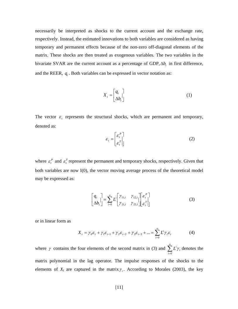
matrix. These shocks are then treated as exogenous variables. The two variables in the
bivariate SVAR are the current account as a percentage of GDP, tbΔ in first difference,
and the REER, . Both variables can be expressed in vector notation as: tq
(1) ⎥⎦
⎤⎢⎣
⎡Δ
=t
tt b
qX
The vector tε represents the structural shocks, which are permanent and temporary,
denoted as:
⎥⎥⎦
⎤
⎢⎢⎣
⎡=
Tt
Pt
t ε
εε (2)
where and represent the permanent and temporary shocks, respectively. Given that
both variables are now I(0), the vector moving average process of the theoretical model
may be expressed as:
Ptε
Ttε
⎥⎥⎦
⎤
⎢⎢⎣
⎡⎥⎦
⎤⎢⎣
⎡=⎥
⎦
⎤⎢⎣
⎡Δ ∑
∞
=Tt
Pt
ii
ii
i
i
t
t Lb
q
ε
εγγγγ
,22,21
,12,11
0
(3)
or in linear form as
∑∞
=−−− =++++=
03322110 ...
iti
ittttt LX εγεγεγεγεγ (4)
where γ contains the four elements of the second matrix in (3) and denotes the
matrix polynomial in the lag operator. The impulse responses of the shocks to the
elements of X
∑∞
=0ii
iL γ
t are captured in the matrix iγ . According to Morales (2003), the key
[11]
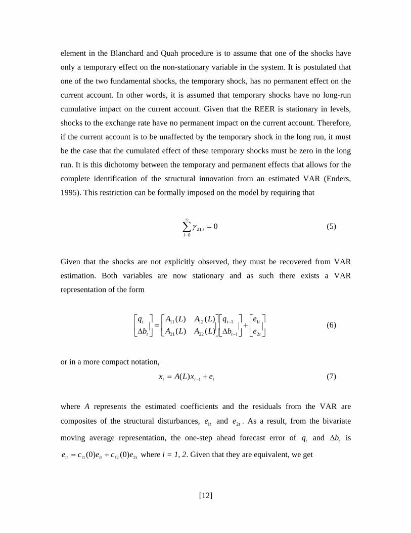
element in the Blanchard and Quah procedure is to assume that one of the shocks have
only a temporary effect on the non-stationary variable in the system. It is postulated that
one of the two fundamental shocks, the temporary shock, has no permanent effect on the
current account. In other words, it is assumed that temporary shocks have no long-run
cumulative impact on the current account. Given that the REER is stationary in levels,
shocks to the exchange rate have no permanent impact on the current account. Therefore,
if the current account is to be unaffected by the temporary shock in the long run, it must
be the case that the cumulated effect of these temporary shocks must be zero in the long
run. It is this dichotomy between the temporary and permanent effects that allows for the
complete identification of the structural innovation from an estimated VAR (Enders,
1995). This restriction can be formally imposed on the model by requiring that
∑∞
−
=0
,21 0i
iγ (5)
Given that the shocks are not explicitly observed, they must be recovered from VAR
estimation. Both variables are now stationary and as such there exists a VAR
representation of the form
⎥⎦
⎤⎢⎣
⎡+⎥
⎦
⎤⎢⎣
⎡Δ⎥
⎦
⎤⎢⎣
⎡=⎥
⎦
⎤⎢⎣
⎡Δ −
−
t
t
t
t
t
t
ee
bq
LALALALA
bq
2
1
1
1
2221
1211
)()()()(
(6)
or in a more compact notation,
ttt exLAx += −1)( (7)
where A represents the estimated coefficients and the residuals from the VAR are
composites of the structural disturbances, and . As a result, from the bivariate
moving average representation, the one-step ahead forecast error of and is
where i = 1, 2. Given that they are equivalent, we get
te1 te2
tq tbΔ
tiitiit ecece 221 )0()0( +=
[12]

⎥⎦
⎤⎢⎣
⎡⎥⎦
⎤⎢⎣
⎡=⎥
⎦
⎤⎢⎣
⎡
t
t
t
t
cccc
ee
2
1
2221
1211
2
1
)0()0()0()0(
εε
(8)
Equation (8) implies that with the help of identifying restrictions, the structural shocks tε
may be recovered from the estimated reduced form disturbances, et as well as the
structural impulse responses iγ from the estimated reduced form VMA coefficients, Ai.
Blanchard and Quah showed that the relationship between (6) and (8), as well as the
long-run restriction outlined in (5) provide exactly four restrictions to identify four
coefficients. These long-run restrictions facilitate the recovery of the underlying
structural disturbances which are used to obtain the impulse responses as well as the
variance decompositions which facilitate the analysis of the dynamic responses of both
variables to the different shocks. Two of these restrictions are normalizations that define
the variance of the structural shocks and . Ptε
Ttε
Restriction 1: (9) 212
2111 )0()0()var( cce t +=
Restriction 2: (10) 222
2212 )0()0()var( cce t +=
Restriction 3: )0()0()0()0(),cov( 2221211121 ccccee tt += (11)
Restriction 4: (12) 0)0()()0()(1 210
12110
22 =+⎥⎦
⎤⎢⎣
⎡− ∑∑
∞
=
∞
=
ckckkk
γγ
The third restriction comes from the assumption that the structural shocks are
orthogonal, while the final restriction is the long-run restriction in (5). This produces the
empirical model:
⎥⎦
⎤⎢⎣
⎡=⎥
⎦
⎤⎢⎣
⎡⎥⎦
⎤⎢⎣
⎡∑∞
= .0..
22,021,0
12,011,0
,22,21
,12,11
0 γγγγ
ii
ii
i
i
AAAA
L (13)
[13]

5.0 Data The series of the current account as a percentage of GDP and the REER for Jamaica are
obtained from the Bank of Jamaica (BOJ) database at the quarterly frequency for the
period 1997 Q1 to 2009 Q3. The current account was seasonally adjusted, denominated
in millions of US dollars and converted to a percentage of the annual nominal GDP. The
series for the REER consists of a weighted average of the local currency relative to a
basket of other currencies of Jamaica’s major trading partners, adjusted for the effects of
inflation. The change in the REER was employed in the paper.
The REER was calculated as follows.
⎟⎟⎠
⎞⎜⎜⎝
⎛×⎟⎠⎞
⎜⎝⎛= ** p
prrREER (14)
where r is the domestic exchange rate, *r is the composite of trading partners’ exchange
rates, p is the domestic price index and is the foreign price index. The base year used
in the REER calculation is 2006.
*p
In the implementation of the Blanchard and Quah methodology, one lag was chosen
based on all criteria except the Schwarz Information Criterion (SIC) that chose zero lags.
Both variables in the model were tested for the presence of unit roots, using the
Augmented Dickey Fuller and Phillips-Perron tests. Unit root test results indicate that the
REER was stationary in levels while stationarity in the current account was achieved
after first differencing (see Table 1, Appendix). Henceforth, a positive temporary shock is
defined as a decline in the policy rate (180-day Treasury bill rate) which would result in
an increase in the demand for foreign currency causing the real exchange rate to
depreciate followed by an improvement in the current account. A positive permanent
shock is defined as a permanent increase in the productive capacity of the domestic
economy thus facilitating an increase in home exports, which would result in an
improvement in the current account balance. As a result, both temporary and permanent
shocks are assumed to have an expansionary impact on the domestic economy.
[14]

6.0 Correlations and Cointegration Tests To determine the historical contribution of temporary and permanent shocks to the REER
and the current account, correlation and cointegration tests were conducted. The
assumption is that if a significant relationship exists between the variable and the
associated shock, then it is indicative that the REER and the current account are driven by
the proposed underlying disturbances. Under the assumption that temporary shocks are
largely monetary shocks and permanent shocks are productivity innovations, the
relationship between the REER and the 180-day Treasury bill (T-bill) rate (proxy for
temporary shock) and the current account and GDP (proxy for permanent shock) was
observed to test for the presence of a long-run relationship between the variables. Table 1
below shows the statistical correlation between the variables and their associated shocks.
Table 1: Correlations
Covariance Analysis: Ordinary Included Observations: 51 Sample: 1997Q1 2009Q3
Correlation t-Statistic Probability
REER T-bill rate REER 1
----- -----
T-bill rate -0.365972 1 -2.752774 ----- 0.0083* ----- Current Account GDP
Current Account 1 ----- -----
GDP 0.583563 1 5.0303 -----
0.0000* ----- *Significant at the 1.0%, 5.0% and 10.0% level.
[15]
Consistent with expectations, the REER and the T-bill rate are negatively correlated with
a correlation coefficient of -0.366 (see Figure 5, Appendix). This indicates moderate
correlation between the variables and the direction suggests that a positive shock to the
interest rate will result in an opposite movement in the REER. Regarding the correlation
between the current account and permanent shocks, proxied by changes in GDP, a
positive correlation of 0.584 was obtained, indicating that movements in these variables
are unidirectional. This suggests that as GDP has persistently decreased over the years
under review, the current account deficit has steadily increased (see Figure 6, Appendix).
For robustness checks, the variables with their associated shocks were tested for
cointegration. Keele and Boef (2004) posited that cointegration implies that the two
integrated series never drift far apart from each other indicating that they maintain
equilibrium. Tables 2a; 2b Appendix, show the results of the Johansen cointegration tests.
Results from the Trace and Max-eigenvalue tests indicate that the REER and current
account are cointegrated with the respective shocks suggesting that the REER and the T-
bill rate are related in the long-run implying that the REER has been largely driven by
temporary shocks while the current account has been largely driven by permanent shocks.
The evidence purported by the above tests lead us to assert that the REER and current
account have been largely driven by temporary and permanent shocks, respectively.
Given this assertion, impulse response analysis is conducted to determine the forecast
direction that the REER and the current account will take in reaction to a positive shock.
7.0 Impulse Responses Impulse responses trace out the response of current and future values of each of the
variables to a one unit increase in the current value of one of the VAR errors, assuming
that this error returns to zero in subsequent periods and that all other errors are equal to
zero. The responses of the variables to a unit positive innovation in each of the shocks
were examined. By incorporating structural decompositions to examine the effects of
both shocks, it was evident that temporary and permanent shocks to both the REER and
the current account partially resulted in the anticipated relationship (see Figure 7,
Appendix). Under temporary shocks, the REER appreciated within the first quarter and
returned to equilibrium by the third quarter. This appreciation in the REER was
[16]

accompanied by a contemporaneous negligible increase in the current account deficit as a
per cent of GDP, consistent with the restrictions imposed in the SVAR. This relationship
between the REER and the current account is consistent with the traditional Mundell-
Fleming theory in the context of an appreciation of the real exchange rate resulting in a
subsequent worsening of the current account deficit. Under the assumption that current
account adjustments to changes in the REER are instantaneous, it should be noted that an
appreciation in the REER is associated with a nominal appreciation in the currency,
which based on theory, results in a loss in competitiveness. This would therefore
contribute to the increase in the current account deficit.
The relationship between the REER and the current account under permanent shocks was
inconsistent with the traditional Mundell-Fleming theory. Based on the monetary
transmission mechanism, an increase in GDP (positive productivity shock) would result
in an initial increase in inflation in the domestic economy. This heightened inflation
would cause interest rates to rise to offset the excess liquidity, resulting in a nominal
depreciation in the exchange rate. This depreciation in the exchange rate would then
result in an improvement in the current account deficit as based on the Marshall-Lerner
condition, the increase in the volume of exports would outweigh the relative price shifts
resulting from the depreciation. However, a one standard deviation positive productivity
shock, resulted in the REER depreciating by approximately 1.0 per cent in the first
quarter and gradually approached equilibrium by the fourth quarter. This change in the
REER was synonymous with a contemporaneous deterioration of the current account
deficit which returned to equilibrium by the fourth quarter. This was inconsistent with
conventional wisdom as it is expected that a depreciation in the REER should be
accompanied by an improvement in the current account deficit. This intuition is based on
the Marshall-Lerner condition being held where it is assumed that exports are elastic
goods which would result in an adjustment being observed contemporaneously. It must
be noted, however, that empirical studies have shown that goods tend to be inelastic in
the short-run as it takes time for consumer preferences to change. Therefore the
Marshall–Lerner condition was not met, and a depreciation may worsen the current
account initially but improve in the long term, as consumers adjust to the new prices.
[17]
A similar model was conducted on data for Trinidad and Tobago for the same review
period. Figure 8, Appendix shows that under temporary shocks to the REER, the
exchange rate appreciated for the first three quarters where it then began to depreciate
until returning to equilibrium in the seventh quarter. The impact of a temporary shock
induced a gradual decline in the current account surplus until the ninth quarter where the
temporary shock had a zero effect. This outturn was consistent with the Mundell-Fleming
theory as a negative correlation between both the REER and the current account surplus
was observed. A positive permanent shock to both variables however, did not display the
expected negative correlation. An increase in the productive capacity of the economy
caused the REER to appreciate while the current account surplus increased. This
deviation from theory was similar to that observed in Jamaica where a negative
correlation was observed between the REER and the current account when influenced by
a permanent shock. One explanation put forward by Lee and Chinn (2005) may be due to
the stationary nature of the current account for Trinidad and Tobago, which would result
in the effect of the permanent shock decaying over time.
It must be noted, however that the temporary and permanent shocks to the variables may
not account for all of the deviation of the actual variables from their long-run equilibrium
values. As recognized by Blanchard and Quah (1989), their model is limited by its ability
to identify only at most as many types of distinct shocks as there are variables. This
suggests that the variables may be affected by other external shocks which are not
captured in the model.
8.0 Variance Decompositions Results from the forecast error variance decomposition indicate how much of the forecast
variation in one variable (for example the current account) departs from its true value due
to variations in the current and future values of the innovations in the other variable (for
example the REER). It therefore indicates the fraction of the forecast error variance at
various horizons that can be attributed to each shock in the model. Table 2 below shows
that at the first horizon, permanent shocks account for 99.1 per cent of the forecast error
[18]

variation in the current account, suggesting that the temporary component accounts for
the remaining 0.9 per cent. Intuitively, after the first forecast horizon, shocks to current
account explained most of its forecast error variation (99.1 per cent), however, after the
second forecast horizon, the REER played a relatively higher role in explaining the
forecast error variation in the current account. Most of the forecast error variation in the
REER is largely explained by its own shocks accounting for approximately 87.0 per cent
within the first forecast horizon and accounting for approximately 83.0 per cent in the
long-run. These results suggest that only approximately a 1.0 per cent correction of the
current account imbalance may be obtained from a real depreciation in the REER in the
first horizon with a correction of 1.7 percentage points being obtained in the long-run.
Table 2: Blanchard-Quah Variance Decomposition: Jamaica Periods Ahead REER Current Account
Temporary
Shock Permanent
Shock Standard
Errors Temporary
Shock Permanent
Shock Standard
Errors 1 86.71 13.29 2.86 0.88 99.12 1.06 2 82.76 17.24 3.02 1.70 98.30 1.10 3 82.80 17.20 3.02 1.70 98.30 1.11 4 82.78 17.22 3.02 1.70 98.30 1.11 5 82.78 17.22 3.02 1.70 98.30 1.11 6 82.78 17.22 3.02 1.71 98.29 1.11 7 82.78 17.22 3.02 1.71 98.29 1.11 8 82.78 17.22 3.02 1.71 98.29 1.11
These results, though consistent with expectations, stand in contrast to those obtained by
Lee and Chinn (2002; 2005). In countries such as Canada, France, and Italy, the
movement of the current account has been largely attributed to temporary shocks given
that the current account has largely been a stationary variable, while the real exchange
rate has been characterized by permanent shocks. The result also suggests that in most
cases a positive and significant relationship between the REER and the current account
will only be found by controlling for permanent shocks to the current account. Indeed
Henry and Longmore (2003), who looked at the short and long-run responses between
both variables, in the Jamaican context, found that the REER could not be used as a tool
for correcting current account imbalances.
[19]

Based on the results, the question may arise in relation to the level at which the Jamaican
current account deficit may then be sustained. Research has indicated that persistent
current account imbalances are unsustainable and pointed to the need for current account
adjustments and even reversals. Rochester (2009) used seven approaches to evaluate the
sustainability of the Jamaican current account. Five out of the seven measures of
sustainability suggested that the Jamaican current account was unsustainable and showed
the need for imminent adjustments in macroeconomic and structural policies. Dean and
Koromzay (1987) posit that current account adjustments can occur mainly through two
mechanisms. The first is based on the determinants of current account transactions,
essentially incomes and relative prices. This, they argue, focuses on rates of growth in
domestic and foreign demand as they influence imports and exports respectively. The
other approach is based on the premise that the current account is identical to the
difference between national saving and investment or the difference between total
domestic demand and output. From this perspective a current-account adjustment can be
analyzed in terms of the determinants of savings and investment behaviour.
9.0 Conclusion and Policy Recommendations An empirical analysis was conducted on the relationship between the REER and the
current account to determine if a current account adjustment may be facilitated by
changes in the REER. Based on the traditional Mundell-Fleming theory and a broad class
of intertemporal macro models, the current account imbalance should be corrected by
depreciation in the real exchange rate given that they are both driven by similar shocks.
The Jamaican current account has exhibited persistent current account deficits, which
have been largely driven by persistently low GDP growth. Similarly, significant
depreciation in the exchange rate has been observed. Despite the considerable
depreciation, a major correction of the current account imbalance has not been observed,
which indicates the need for structural changes in the economy. Cointegration analysis
and variance decompositions indicated that temporary shocks played a larger role in
explaining the variation in the REER, while the current account was largely driven by
[20]

permanent shocks. It has been argued that persistent current account imbalances are
unsustainable and an adjustment deemed necessary. Over the past decade, the real sector
in the Jamaican economy has not been able to facilitate the necessary adjustment that
should take place from the REER to the current account. It has also been proven
econometrically that the relatively small significance of the temporary component in the
current account, suggests that a significant adjustment of the current account would not
occur through a REER adjustment. We therefore conclude that this adjustment in the
current account imbalance may not be entirely achieved through the manipulation of
monetary variables such as interest rates but rather through enhancing the
macroeconomic environment to increase productivity. Under the assumption that the
Marshall-Lerner condition holds, a boost to productivity would cause exports to increase
and the demand for imports to fall. In this regard, policy should be more geared towards
creating a macro-economic environment that can facilitate the increase in exports
resulting in a boost in external competitiveness which would then cause a correction in
the current account imbalance.
[21]

10. References
Beveridge, S. and C. Nelson (1981), “A New Approach to Decomposition of Economic Time Series into Permanent and Transitory Components with Particular Attention to Measurement of the Business Cycle”, Journal of Monetary Economics, Vol.7, 151-174. Blanchard, O. and Daniel Quah (1989), “The Dynamic Effects of Aggregate Demand and Supply Disturbances” American Economic Review, Vol. 79, No.4, September. Cavallari, Lilia (1999), “Current Account and Exchange Rate Dynamics”, University of Rome, “La Sapienza” ”, July. Clarida, Richard and Jordi Gali (1994), “Sources of Real Exchange Rate Fluctuations: How Important are Nominal Shocks?” NBER Working Paper Series No. 4658, February. Dean, Andrew and Val Koromzay (1987), “Current Account Imbalances and Adjustment Mechanisms”, OECD Economic Studies 8 (Spring). De Silva, Ashton (2007), “A Multivariate Innovations State Space Beveridge Nelson Decomposition”, Munich Personal RePEc Archive, RMIT University, October.
Erlat, Haluk and Guzin Erlat (1998), “Permanent and Transitory Shocks on Real and Nominal Exchange Rates in Turkey during the post-1980 Period”, Atlantic Economic Journal, Vol. 26, No. 4, December. Gauthier, Celine and David Tessier (2002), “Supply Shocks and Real Exchange Rate Dynamics: Canadian Evidence”, Bank of Canada Working Paper, November. Gottschalk, Jan and Willem Van Zandweghe (2001), “Do Bivariate SVAR Models with Long-Run Identifying Restrictions Yield Reliable Results? The Case of Germany”, Kiel Working Paper, No. 1068, Kiel Institute of World Economics. Henry, Chandar and Rohan Longmore (2003), “Current Account Dynamics and the Real Effective Exchange Rate: The Jamaican Experience”, Bank of Jamaica Research Paper, March. Hossain, Ferdaus (1999), “Transitory and Permanent Disturbances and the Current Account: An Empirical Analysis in the Intertemporal Framework”, Applied Economics, Vol. 31, Issue 8, August. Huizinga, John (1987), “The Empirical Investigation of the Long-Run Behaviour of Real Exchange Rates”, Carnegie-Rochester Conference Series on Public Policy, Vol. 27, Autumn.
[22]

Keating, John W and John V. Nye (1998), “Permanent and Transitory Shocks in Real Output: Estimates from Nineteenth-Century and Postwar Economies”, Journal of Money, Credit and Banking, Vol. 30, No. 2. Kwalingana, Samson and Nkuna, Onelie (2009) “The Determinants of Current Account Imbalances in Malawi”, Munich Personal RePEc Archive, April. Lastrapes, W.D., (1992), “Sources of Fluctuations in Real and Nominal Exchange Rates” Review of Economics & Statistics, Vol. 74, 530-9. Lee, Jaewoo and Menzie D. Chinn (1998), “The Current Account and the Real Exchange Rate: A Structural VAR Analysis of Major Currencies”, NBER Working Paper Series No. 6495, April. Lee, Jaewoo and Menzie D. Chinn (2002), “Current Account and Real Exchange Rate Dynamics in the G-7 Countries” IMF Working Paper, August. Lee, Jaewoo and Menzie D. Chinn (2005), “Three Current Account Balances: A Semi-Structuralist” Interpretation”, NBER Working Paper No. 11853, December. McDonald, Ronald (1998), “What do we really know about Real Exchange Rates?” Working Paper 28, Austrian Central Bank, June. Morales, Marco (2003), “Dynamic Interaction for Andean Countries: Evidence from VAR Approach”, ECLAC, October. Nelson, Charles R., (2006), “The Beveridge-Nelson Decomposition in Retrospect and Prospect”, Journal of Econometrics, Vol. 146, Issue 2, October. Rochester, Lance (2009), “Revisiting Current Account Sustainability Measures for Jamaica: An Assessment”, Bank of Jamaica Working Paper, April. Rogers, John H. (1998), “Monetary Shocks and Real Exchange Rates”, Board of Governors of the Federal Reserve System, International Finance Discussion Papers, 612. Stockman, Alan C., (1978), “A Theory of Exchange Rate Determination”, University of California Discussion Paper 122, June. Wang, Tao (2004), “China: Sources of Real Exchange Rate Fluctuations”, IMF Working Paper, February. Zhang, Yanchun (2009), “The Role of Monetary Shocks and Real Shocks on the Current Account, the Terms of Trade and the Real Exchange Rate Dynamics: a SVAR Analysis”. Applied Economics, Vol. 41, Issue 16, July.
[23]

APPENDIX
Figure 1a: Current Account as Per Cent of GDP - Advanced Economies
-12-10-8-6-4-20246
1997 1998 1999 2000 2001 2002 2003 2004 2005 2006 2007 2008 2009
Year
Per C
ent (
%)
Canada France UK USA
Figure 1b: Current Account as Per Cent of GDP - Developing Economies
-30
-20
-100
10
20
3040
50
60
1997 1998 1999 2000 2001 2002 2003 2004 2005 2006 2007 2008 2009
Year
Per C
ent (
%)
Jamaica T&T Venezuela Mexico
[24]

Figure 2: Jamaica's Trade Balance
0.0
1000.0
2000.0
3000.0
4000.0
5000.0
6000.0
7000.0
8000.0
1996 1997 1998 1999 2000 2001 2002 2003 2004 2005 2006 2007 2008 2009
Year
US$
'000
Total Exports Total Imports (fob)
Figure 3: Jamaica's Current Account as a Per Cent of GDP
1.7
4.2
4.12.3
3.7
8.0
10.49.1
5.0
9.6
9.9
15.7
19.5
7.4
0.00
5.00
10.00
15.00
20.00
25.00
1996 1997 1998 1999 2000 2001 2002 2003 2004 2005 2006 2007 2008 2009
Year
Per c
ent (
%)
[25]

Figure 4: Jamaica's REER Index and Current Account as a Percentage of GDP
0.0
5.0
10.0
15.0
20.0
25.0
1996
1997
1998
1999
2000
2001
2002
2003
2004
2005
2006
2007
2008
2009
Year
80.085.090.095.0100.0105.0110.0
CA/GDP REER
Table 1: Unit root Tests ADF* Phillips-Perron*
Variables Level First Difference Level First Difference CAGDP -2.85 -9.00 -2.81 -9.00 REER -5.11 -7.29 -4.86 -22.05
* Without trend
Critical values: 1% 3.57
5% 2.92
[26]

Figure 5: REER and 180-day T-bill Rate
-20.00
-15.00
-10.00
-5.00
0.00
5.00
10.00
15.00
Mar
-96
Mar
-97
Mar
-98
Mar
-99
Mar
-00
Mar
-01
Mar
-02
Mar
-03
Mar
-04
Mar
-05
Mar
-06
Mar
-07
Mar
-08
Mar
-09
Month
0.005.0010.00
15.0020.0025.0030.00
35.0040.0045.00
REER GOJ 180-day T-bill rate
Figure 6: Current Account and GDP
-1000
-800
-600
-400
-200
0
200
Jun-
97Ju
n-98
Jun-
99Ju
n-00
Jun-
01Ju
n-02
Jun-
03Ju
n-04
Jun-
05Ju
n-06
Jun-
07Ju
n-08
Jun-
09
Month
0
500
1000
1500
2000
2500
3000
3500
Current Account GDP
[27]

Table 2a: Johansen Cointegration Test (REER and T-bill rate)
Unrestricted Cointegration Rank Test (Trace)
Hypothesized Trace 0.05 No. of CE(s) Eigenvalue Statistic Critical Value Prob.**
None * 0.372154 23.10612 12.32090 0.0006 At most 1 0.006075 0.298584 4.129906 0.6462
Trace test indicates 1 cointegrating eqn(s) at the 0.05 level * denotes rejection of the hypothesis at the 0.05 level Unrestricted Cointegration Rank Test (Maximum Eigenvalue)
Hypothesized Max-Eigen 0.05 No. of CE(s) Eigenvalue Statistic Critical Value Prob.**
None * 0.372154 22.80754 11.22480 0.0003 At most 1 0.006075 0.298584 4.129906 0.6462
Max-eigenvalue test indicates 1 cointegrating eqn(s) at the 0.05 level * denotes rejection of the hypothesis at the 0.05 level
Table 2b: Johansen Cointegration Test (Current Account and GDP)
Unrestricted Cointegration Rank Test (Trace)
Hypothesized Trace 0.05 No. of CE(s) Eigenvalue Statistic Critical Value Prob.**
None * 0.276062 19.41643 12.32090 0.0028 At most 1 0.070589 3.587015 4.129906 0.0691
Trace test indicates 1 cointegrating eqn(s) at the 0.05 level * denotes rejection of the hypothesis at the 0.05 level Unrestricted Cointegration Rank Test (Maximum Eigenvalue)
Hypothesized Max-Eigen 0.05 No. of CE(s) Eigenvalue Statistic Critical Value Prob.**
None * 0.276062 15.82941 11.22480 0.0073 At most 1 0.070589 3.587015 4.129906 0.0691
Max-eigenvalue test indicates 1 cointegrating eqn(s) at the 0.05 level * denotes rejection of the hypothesis at the 0.05 level
[28]

Figure 7: Response to Structural One S.D. Innovations: Jamaica
-2
-1
0
1
2
3
1 2 3 4 5 6 7 8
Response of REER to Temporary Shock
-2
-1
0
1
2
3
1 2 3 4 5 6 7 8
Response of REER to Permanent Shock
-.4
-.2
.0
.2
.4
1 2 3 4 5 6 7 8
Response of Current Account to Temporary Shock
-0.4
0.0
0.4
0.8
1.2
1 2 3 4 5 6 7 8
Response of Current Accountto Permanent Shock
[29]

Figure 8: Response to Structural One S.D. Innovations: Trinidad and Tobago
-1.0
-0.5
0.0
0.5
1.0
1.5
1 2 3 4 5 6 7 8 9 10 11 12
Response of REER to Permanent Shock
-1.0
-0.5
0.0
0.5
1.0
1.5
1 2 3 4 5 6 7 8 9 10 11 12
Response of REER to Temporary Shock
-0.4
0.0
0.4
0.8
1.2
1.6
1 2 3 4 5 6 7 8 9 10 11 12
Response of Current Account toPermanent Shock
-0.4
0.0
0.4
0.8
1.2
1.6
1 2 3 4 5 6 7 8 9 10 11 12
Response of Current Account toTemporary Shock
[30]