Exploring Statistics
33
-
Upload
yet-barreda-basbas -
Category
Documents
-
view
215 -
download
0
Transcript of Exploring Statistics

7/28/2019 Exploring Statistics
http://slidepdf.com/reader/full/exploring-statistics 1/33

7/28/2019 Exploring Statistics
http://slidepdf.com/reader/full/exploring-statistics 2/33
STATISTICS
Help decision makers extract
maximum usefulness from
limited information
• FACILITATE WISE DECISION IN THE FACE OF UNCERTAINTY

7/28/2019 Exploring Statistics
http://slidepdf.com/reader/full/exploring-statistics 3/33
DESCRIPTIVE STATISTICS
Techniques for the collection
and effective presentation of numerical information
• GIVE INFORMATION OR DESCRIBE THE SAMPLE
MEAN
VARIANCE
STANDARD DEVIATION
7/28/2019 Exploring Statistics
http://slidepdf.com/reader/full/exploring-statistics 4/33
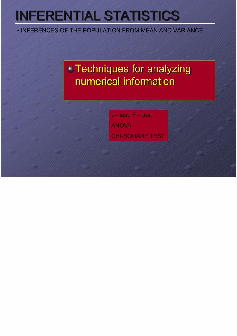
INFERENTIAL STATISTICS
Techniques for analyzing
numerical information
• INFERENCES OF THE POPULATION FROM MEAN AND VARIANCE
t – test; F – test
ANOVA
CHI-SQUARE TEST
7/28/2019 Exploring Statistics
http://slidepdf.com/reader/full/exploring-statistics 5/33
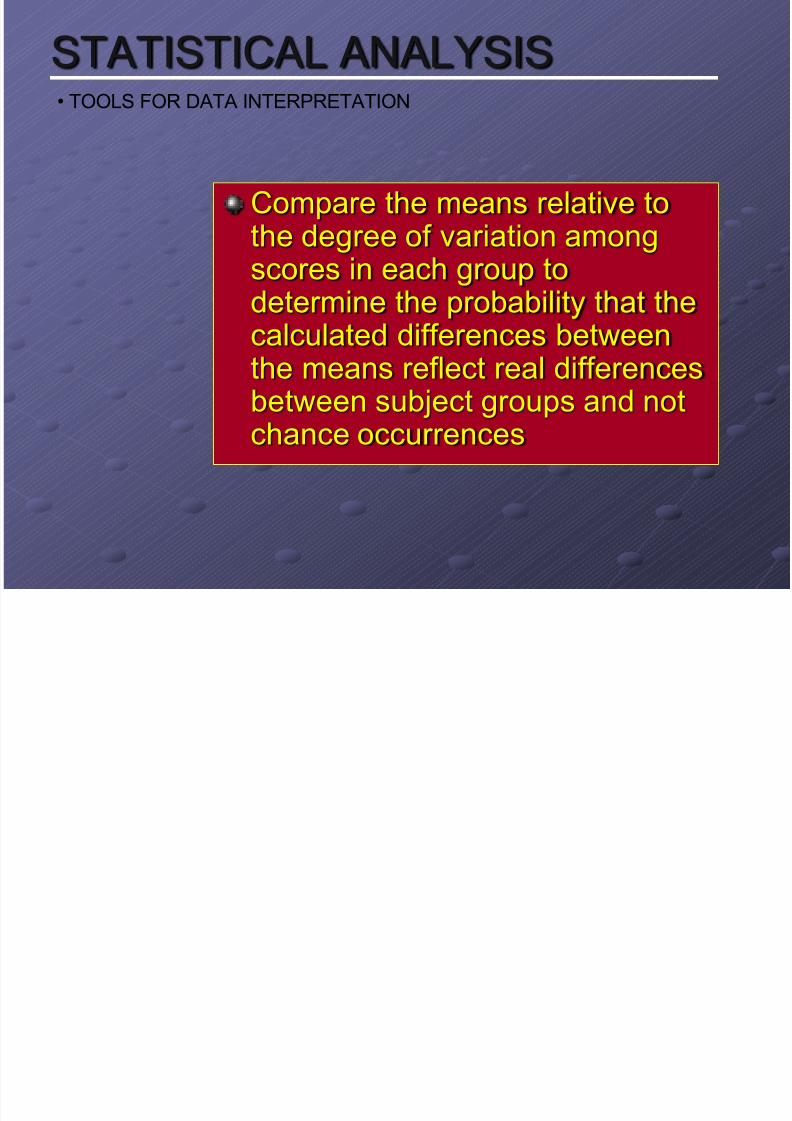
STATISTICAL ANALYSIS
Compare the means relative tothe degree of variation among
scores in each group todetermine the probability that thecalculated differences betweenthe means reflect real differences
between subject groups and notchance occurrences
• TOOLS FOR DATA INTERPRETATION

7/28/2019 Exploring Statistics
http://slidepdf.com/reader/full/exploring-statistics 6/33
STATISTICAL ANALYSIS
Difference between two
means is significant at 0.05level of significance implies a
probability of less than 5 out
of 100 that the difference isdue to chance
• TOOLS FOR DATA INTERPRETATION

7/28/2019 Exploring Statistics
http://slidepdf.com/reader/full/exploring-statistics 7/33
DESCRIPTIVE STATISTICS• WHAT IS BEING DESCRIBED
Level of
measurement
Central
Tendency
Dispersion/
Variability
Relationship
NOMINAL Mode - Contingency
coefficientORDINAL Median
Mode
Range Rank order
correlation coef.
INTERVAL/
RATIO
Mean
MedianMode
Standard Dev.
VarianceRange
Pearson product
moment
correlation
7/28/2019 Exploring Statistics
http://slidepdf.com/reader/full/exploring-statistics 8/33
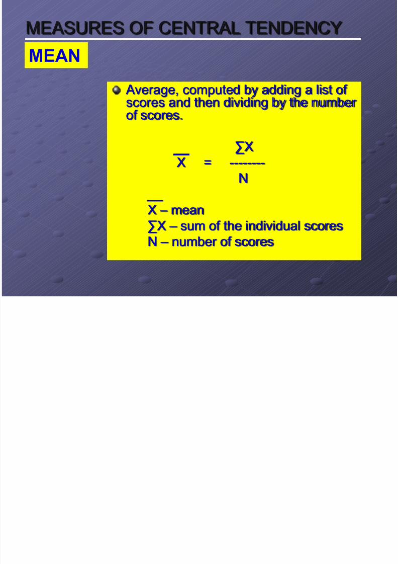
MEASURES OF CENTRAL TENDENCY
Average, computed by adding a list of scores and then dividing by the number of scores.
∑X
X = --------
N
X – mean∑X – sum of the individual scores
N – number of scores
MEAN

7/28/2019 Exploring Statistics
http://slidepdf.com/reader/full/exploring-statistics 9/33
MEASURES OF DISPERSION
Measure of the spread of a set of scores
N∑X2 – (∑X)2
s = --------------------
N(N – 1)
s – standard deviation∑X – sum of the individual scores
N – number of scores
STANDARD DEVIATION

7/28/2019 Exploring Statistics
http://slidepdf.com/reader/full/exploring-statistics 10/33
INFERENTIAL STATISTICS• DEPEND ON HYPOTHESES AND SCALE OF VARIABLE
STATISTICAL TEST HYPOTHESIS TESTED
t - test About a single mean
Difference between 2 means
One-way ANOVA Two or more population means
are equal – single independent
variableTwo-way ANOVA Two or more population means
are equal – two independent
variables
PARAMETRIC TESTS

7/28/2019 Exploring Statistics
http://slidepdf.com/reader/full/exploring-statistics 11/33
PARAMETRIC TEST
Normal distribution
Homogeneity of variance
Continuous equal interval
measures
• EMPLOY INTERVAL MEASUREMENT OF THE DEPENDENT VARIABLE
7/28/2019 Exploring Statistics
http://slidepdf.com/reader/full/exploring-statistics 12/33
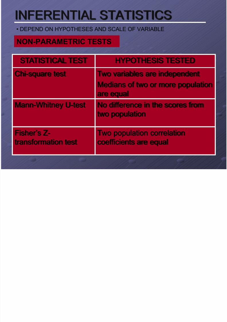
INFERENTIAL STATISTICS• DEPEND ON HYPOTHESES AND SCALE OF VARIABLE
STATISTICAL TEST HYPOTHESIS TESTED
Chi-square test Two variables are independent
Medians of two or more population
are equal
Mann-Whitney U-test No difference in the scores from
two population
Fisher’s Z-
transformation test
Two population correlation
coefficients are equal
NON-PARAMETRIC TESTS
7/28/2019 Exploring Statistics
http://slidepdf.com/reader/full/exploring-statistics 13/33
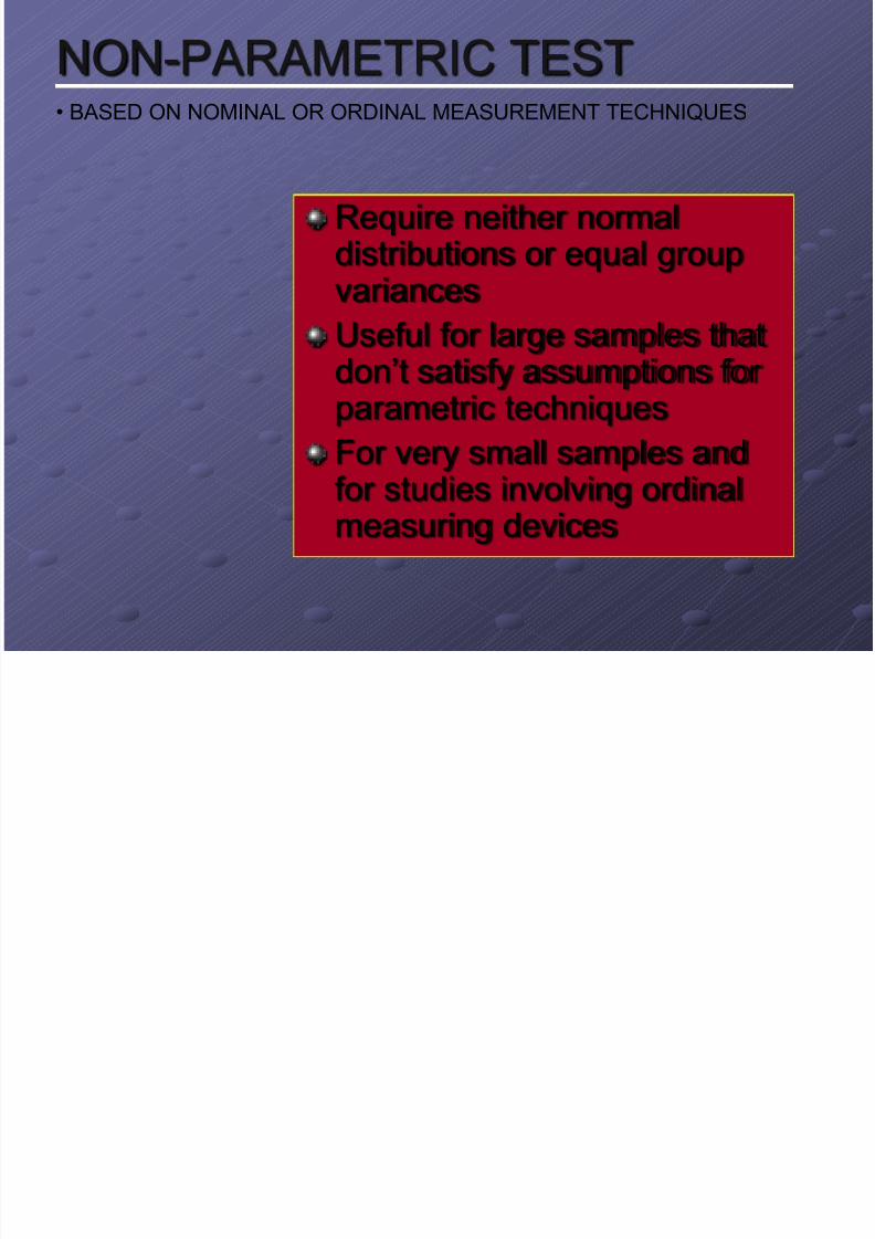
NON-PARAMETRIC TEST
Require neither normaldistributions or equal group
variancesUseful for large samples thatdon’t satisfy assumptions for parametric techniques
For very small samples andfor studies involving ordinalmeasuring devices
• BASED ON NOMINAL OR ORDINAL MEASUREMENT TECHNIQUES

7/28/2019 Exploring Statistics
http://slidepdf.com/reader/full/exploring-statistics 14/33
SELECTING A STATISTICAL TEST
TYPE AND NUMBER OF INDEPENDENT VARIABLES
INTERVAL ORDINAL NOMINAL
1 More Than 1 1 More Than 1 1 More Than 1
TypeAnd
Number
Of
DependentVariables
INTERVAL 0 - Factor Analysis
Transform ordinal variable intonominal and use C-1, or; Transform the interval variable
into ordinal and use B-2, or; Transform both variables intonominal and use C-3.
- - ROW1
1 Correlation Multiple
Correlation
Analysis of
Variance, or
t-Test
Analysis of
Variance
More
Than 1
Multiple
Correlation
- - -
ORDINAL 0 Transform ordinal variable into
nominal and use C-1, or; Transform the interval variable
into ordinal and use B-2, or; Transform the interval variableinto nominal and use C-2.
- Coefficient of
Concordance(W)
- - ROW
2
1 Spearman
Correlation,Kendall’s T
- Sign Test,
Median Test,U-Test,
Kruskal-Wallis
Friedman’s
Two-Way Analysis of
Variance
More
Than 1 - - - -
NOMINAL 0 - - - - - Chi-Square ROW
3
1 Analysis of Variance
- Sign Test,Median Test,
U-Test,
Kruskal-Wallis
- Phi Coeff. Ø, Fisher Exact
Test,
Chi-Square
-
More
Than 1 Analysis of
Variance- Friedman’s
Two-Way
Analysis of
Variance
- - -
COLUMN A COLUMN B COLUMN C
7/28/2019 Exploring Statistics
http://slidepdf.com/reader/full/exploring-statistics 15/33
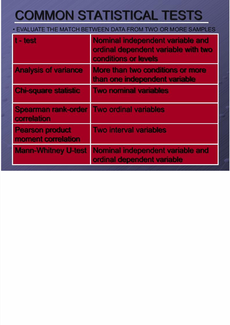
COMMON STATISTICAL TESTS• EVALUATE THE MATCH BETWEEN DATA FROM TWO OR MORE SAMPLES
t - test Nominal independent variable andordinal dependent variable with two
conditions or levels
Analysis of variance More than two conditions or more
than one independent variableChi-square statistic Two nominal variables
Spearman rank-order
correlation
Two ordinal variables
Pearson product
moment correlation
Two interval variables
Mann-Whitney U-test Nominal independent variable and
ordinal dependent variable
7/28/2019 Exploring Statistics
http://slidepdf.com/reader/full/exploring-statistics 16/33
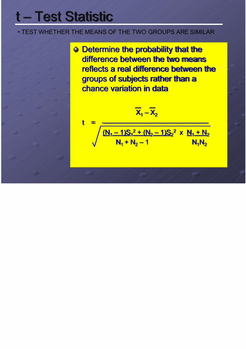
t – Test Statistic
Determine the probability that the
difference between the two means
reflects a real difference between the
groups of subjects rather than a
chance variation in data
X1 – X2
t = -----------------------------------------------
(N1 – 1)S12 + (N2 – 1)S2
2 x N1 + N2
N1 + N2 – 1 N1N2
• TEST WHETHER THE MEANS OF THE TWO GROUPS ARE SIMILAR
7/28/2019 Exploring Statistics
http://slidepdf.com/reader/full/exploring-statistics 17/33
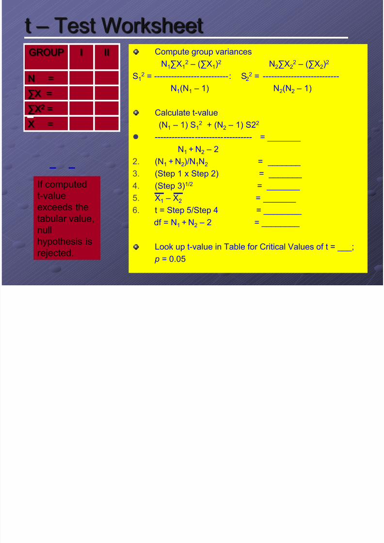
t – Test WorksheetCompute group variances
N1∑X1
2
– (∑X1)
2
N2∑X2
2
– (∑X2)
2
S1
2 = --------------------------: S22 = ---------------------------
N1(N1 – 1) N2(N2 – 1)
Calculate t-value
(N1 – 1) S12 + (N2 – 1) S22
---------------------------------- = _______
N1 + N2 – 2
2. (N1 + N2)/N1N2 = _______
3. (Step 1 x Step 2) = _______
4. (Step 3)1/2 = _______
5. X1 – X2 = _______ 6. t = Step 5/Step 4 = ________
df = N1 + N2 – 2 = ________
Look up t-value in Table for Critical Values of t = ___;
p = 0.05
GROUP I II
N =
∑X =
∑X2 =
X =
If computed
t-value
exceeds the
tabular value,
null
hypothesis is
rejected.
7/28/2019 Exploring Statistics
http://slidepdf.com/reader/full/exploring-statistics 18/33
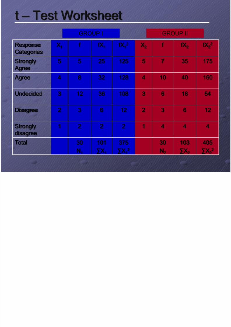
t – Test Worksheet
Response
Categories
X1 f fX1 fX12 X2 f fX2 fX2
2
Strongly
Agree
5 5 25 125 5 7 35 175
Agree 4 8 32 128 4 10 40 160
Undecided 3 12 36 108 3 6 18 54
Disagree 2 3 6 12 2 3 6 12
Strongly
disagree
1 2 2 2 1 4 4 4
Total 30
N1
101
∑X1
375
∑X12
30
N2
103
∑X2
405
∑X22
GROUP IIGROUP I

7/28/2019 Exploring Statistics
http://slidepdf.com/reader/full/exploring-statistics 19/33
t – Test WorksheetCompute group variances
N1∑X1
2
– (∑X1)
2
N2∑X2
2
– (∑X2)
2
S1
2 = --------------------------: S22 = ---------------------------
N1(N1 – 1) N2(N2 – 1)
S12 = 1.21 S2
2 = 1.77
Calculate t-value
(N1 – 1) S12 + (N2 – 1) S22
---------------------------------- = 1.49
N1 + N2 – 2
2. (N1 + N2)/N1N2 = 0.07
3. (Step 1 x Step 2) = 0.104
4. (Step 3)1/2 = 0.32
5. X1 – X2 = 0.066. t = Step 5/Step 4 = 0.1875
df = N1 + N2 – 2 = 58
Look up t-value in Table for Critical Values of t = 2.00
p = 0.05
GROUP I II
N = 30 30
∑X = 101 103
∑X2 = 375 405
X = 3.37 3.43
If computed
t-value
exceeds the
tabular value,
null
hypothesis is
rejected.
7/28/2019 Exploring Statistics
http://slidepdf.com/reader/full/exploring-statistics 20/33
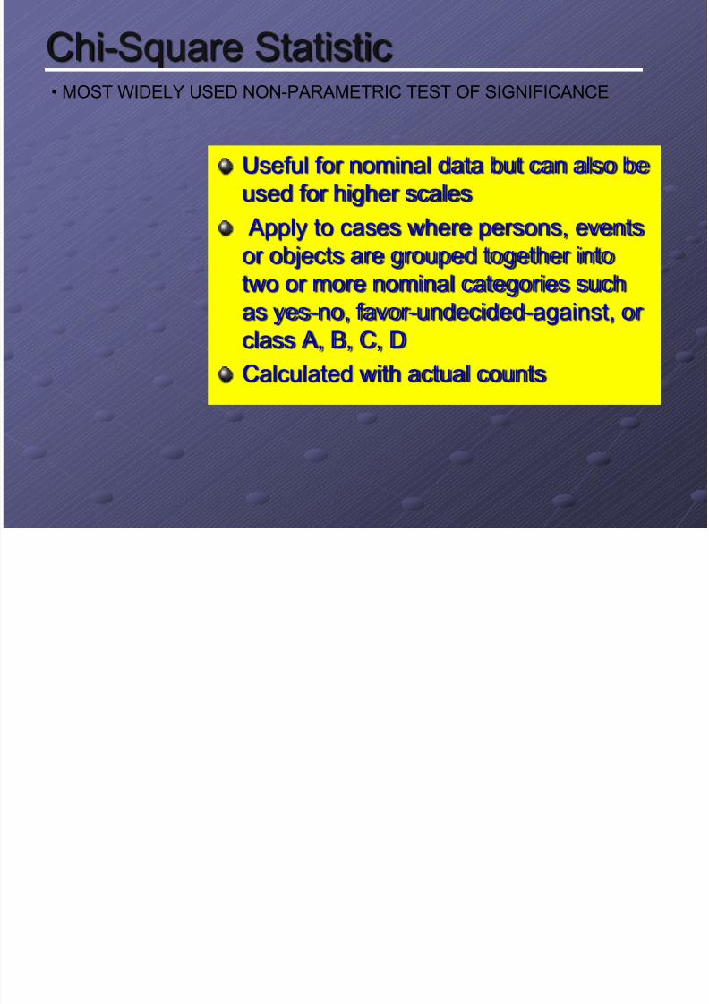
Chi-Square Statistic
Useful for nominal data but can also be
used for higher scales
Apply to cases where persons, events
or objects are grouped together intotwo or more nominal categories such
as yes-no, favor-undecided-against, or
class A, B, C, D
Calculated with actual counts
• MOST WIDELY USED NON-PARAMETRIC TEST OF SIGNIFICANCE

7/28/2019 Exploring Statistics
http://slidepdf.com/reader/full/exploring-statistics 21/33
Chi-Square Statistic
Applied to test of significance between
the observed distribution of data
among categories and expected
distributionExamine questions of relationship
Used in one-sample analysis, two
independent samples, or
k-independent samples
• MOST WIDELY USED NON-PARAMETRIC TEST OF SIGNIFICANCE

7/28/2019 Exploring Statistics
http://slidepdf.com/reader/full/exploring-statistics 22/33
Chi-Square Statistic
FORMULA:
(Oi – Ei)2
ϰ2 = ∑ -------------
Ei
O – observed frequencies
E – expected frequencies
• ONE-SAMPLE CASE ANALYSIS
k
i = 1
7/28/2019 Exploring Statistics
http://slidepdf.com/reader/full/exploring-statistics 23/33
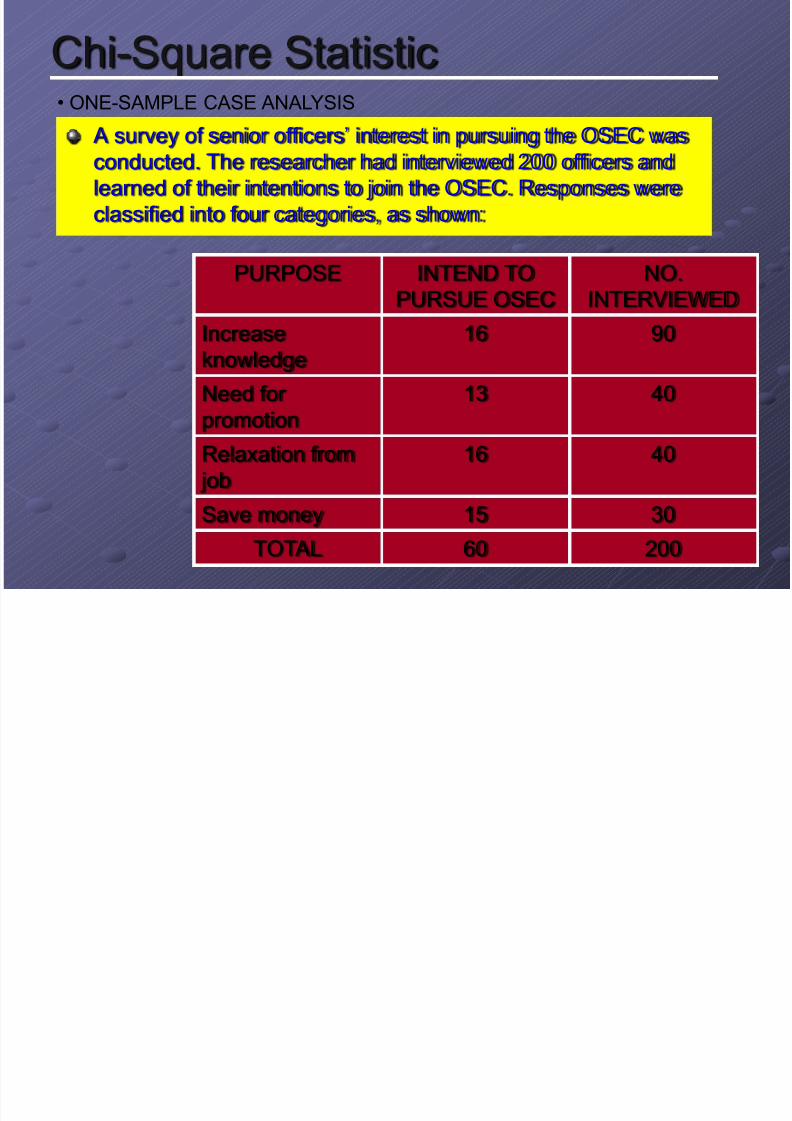
Chi-Square Statistic
A survey of senior officers’ interest in pursuing the OSEC wasconducted. The researcher had interviewed 200 officers and
learned of their intentions to join the OSEC. Responses were
classified into four categories, as shown:
• ONE-SAMPLE CASE ANALYSIS
PURPOSE INTEND TOPURSUE OSEC
NO.INTERVIEWED
Increase
knowledge
16 90
Need for
promotion
13 40
Relaxation from
job
16 40
Save money 15 30
TOTAL 60 200
7/28/2019 Exploring Statistics
http://slidepdf.com/reader/full/exploring-statistics 24/33
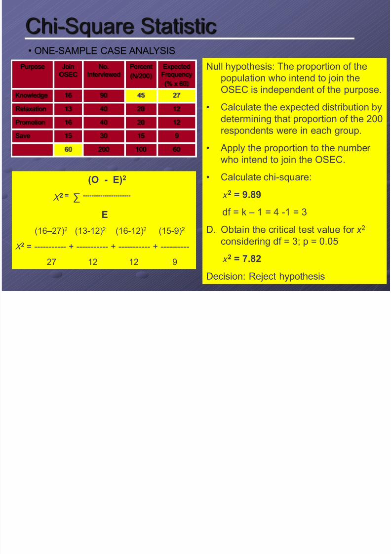
Chi-Square Statistic• ONE-SAMPLE CASE ANALYSIS
Purpose JoinOSEC No.Interviewed Percent(N/200)
ExpectedFrequency
(% x 60)
Knowledge 16 90 45 27
Relaxation 13 40 20 12
Promotion 16 40 20 12
Save 15 30 15 9
60 200 100 60
Null hypothesis: The proportion of thepopulation who intend to join the
OSEC is independent of the purpose.
• Calculate the expected distribution by
determining that proportion of the 200
respondents were in each group.
• Apply the proportion to the number
who intend to join the OSEC.
• Calculate chi-square:
x 2 = 9.89
df = k – 1 = 4 -1 = 3
D. Obtain the critical test value for x 2
considering df = 3; p = 0.05
x 2 = 7.82
Decision: Reject hypothesis
(O - E)2
X 2 = ∑ ----------------------
E
(16 –27)2 (13-12)2 (16-12)2 (15-9)2
X 2 = ----------- + ----------- + ----------- + ----------
27 12 12 9
7/28/2019 Exploring Statistics
http://slidepdf.com/reader/full/exploring-statistics 25/33
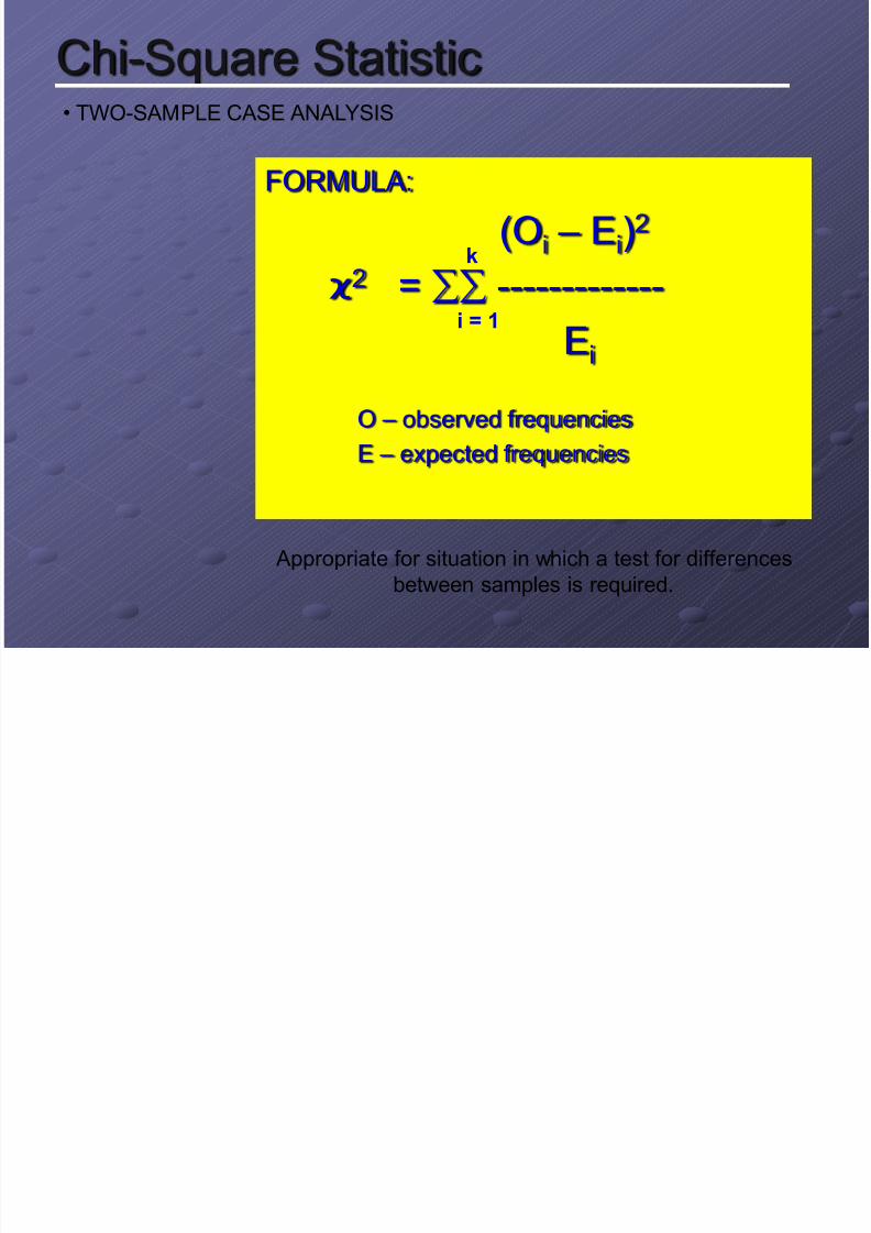
Chi-Square Statistic
FORMULA:
(Oi – Ei)2
ϰ2 = ∑∑ -------------
Ei
O – observed frequencies
E – expected frequencies
• TWO-SAMPLE CASE ANALYSIS
k
i = 1
Appropriate for situation in which a test for differences
between samples is required.
7/28/2019 Exploring Statistics
http://slidepdf.com/reader/full/exploring-statistics 26/33
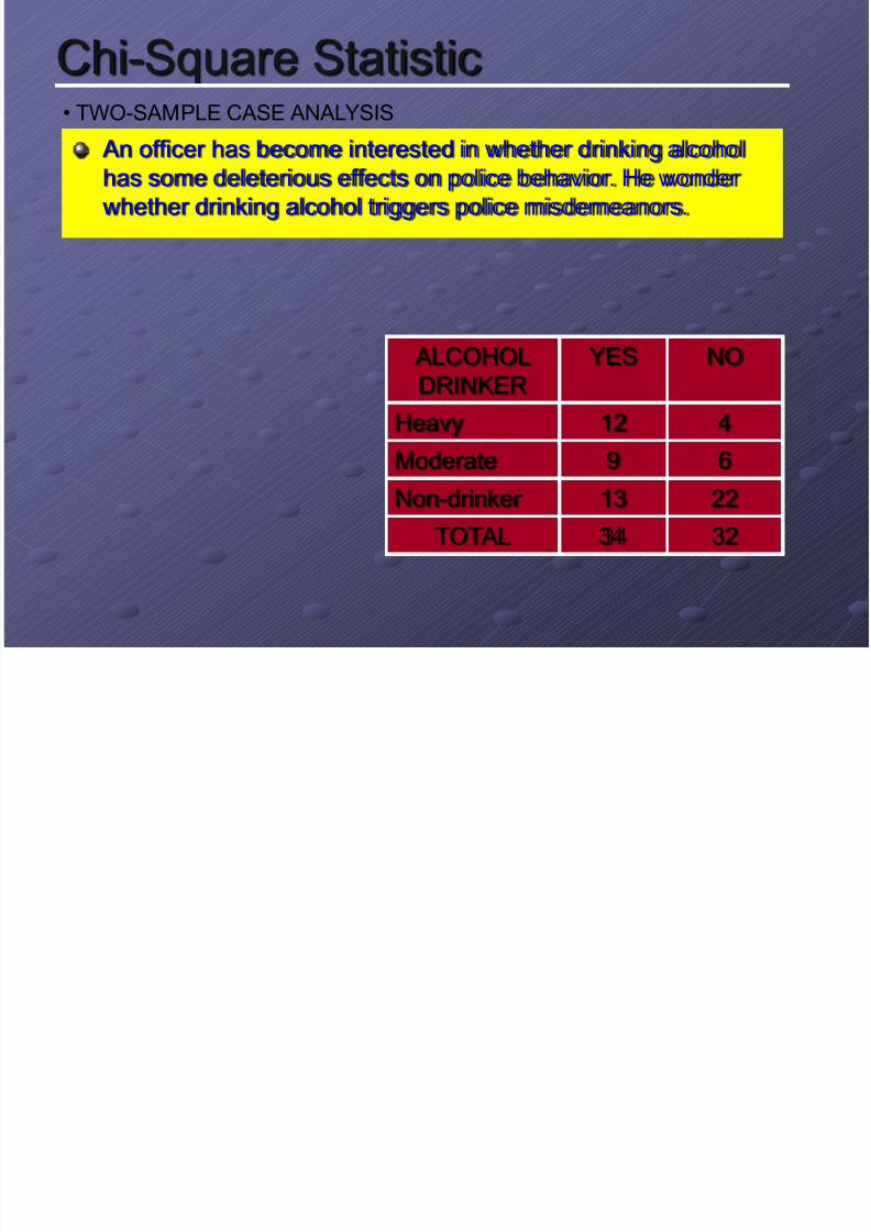
Chi-Square Statistic
An officer has become interested in whether drinking alcoholhas some deleterious effects on police behavior. He wonder
whether drinking alcohol triggers police misdemeanors.
• TWO-SAMPLE CASE ANALYSIS
ALCOHOL
DRINKER
YES NO
Heavy 12 4
Moderate 9 6
Non-drinker 13 22
TOTAL 34 32

7/28/2019 Exploring Statistics
http://slidepdf.com/reader/full/exploring-statistics 27/33
Chi-Square Statistic
AlcoholDrinker YES NO Row Total
Heavy 12 4 16
Moderate 9 6 15
Non-drinker 13 22 35
Column
Total
34 32 66
• TWO SAMPLE CASE ANALYSISNull hypothesis: There is no difference in
police misdemeanor occurrencesbetween alcohol drinker and non-
drinker.
• Calculate the expected observations
in each cell by multiplying the two
marginal totals common to aparticular cell and dividing this
product by the total observations.
• Calculate chi-square:
x 2 = 6.86
df = (r – 1)(c – 1) = (3-1)(2-1) = 2
D. Obtain the critical test value for x 2
considering df = 2; p = 0.05
x 2 = 5.99
Decision: Reject hypothesis
(12 –8.24)2 (9-7.73)2 (13-18.03)2 (4-7.76)2 (6-7.27)2 (22-16.97)2
X 2 = ------------ + ----------- + --------------- + ----------- + ---------- + --------------
8.24 7.73 18.03 7.76 7.27 16.97
Alcohol
Drinker
YES NO Row Total
Heavy 8.24 7.76 16
Moderate 7.73 7.27 15
Non-drinker 18.03 16.97 35
Column
Total
34 32 66
7/28/2019 Exploring Statistics
http://slidepdf.com/reader/full/exploring-statistics 28/33
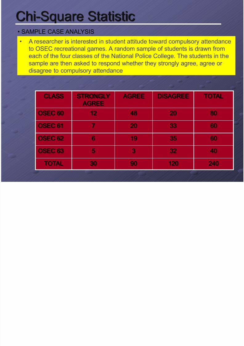
Chi-Square Statistic• SAMPLE CASE ANALYSIS
• A researcher is interested in student attitude toward compulsory attendanceto OSEC recreational games. A random sample of students is drawn from
each of the four classes of the National Police College. The students in the
sample are then asked to respond whether they strongly agree, agree or
disagree to compulsory attendance
CLASS STRONGLY
AGREE
AGREE DISAGREE TOTAL
OSEC 60 12 48 20 80
OSEC 61 7 20 33 60
OSEC 62 6 19 35 60
OSEC 63 5 3 32 40
TOTAL 30 90 120 240

7/28/2019 Exploring Statistics
http://slidepdf.com/reader/full/exploring-statistics 29/33
Chi-Square Statistic
CLASS SD A D TOTAL
O-60 12 48 20 80
O-61 7 20 33 60
O-62 6 19 35 60
O-63 5 3 32 40
TOTAL 30 90 120 240
• SAMPLE CASE ANALYSIS
Null Hypothesis: The four class
populations do not differ in their
attitude toward compulsory attendance
to OSEC recreational games.
• Determine the value of the expected
outcome, E = (∑k∑r)/N
• Compute chi-square value:x 2 = 40.28
df = (r – 1)(c – 1) = 6
C. Obtain the critical test value:
x 2 = 12.59
p = 0.05
Conclusion: Class and attitude toward
compulsory attendance to OSEC
recreational games are related (not
independent) in the student population.
The null hypothesis is rejected.
CLASS SD A D TOTAL
O-60 10 30 40 80
O-61 7.5 22.5 30 60
O-62 7.5 22.5 30 60
O-63 5 15 20 40
TOTAL 30 90 120 240
7/28/2019 Exploring Statistics
http://slidepdf.com/reader/full/exploring-statistics 30/33
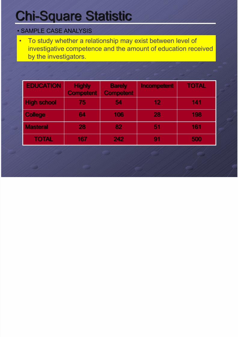
Chi-Square Statistic• SAMPLE CASE ANALYSIS
• To study whether a relationship may exist between level of investigative competence and the amount of education received
by the investigators.
EDUCATION HighlyCompetent
BarelyCompetent
Incompetent TOTAL
High school 75 54 12 141
College 64 106 28 198
Masteral 28 82 51 161
TOTAL 167 242 91 500
7/28/2019 Exploring Statistics
http://slidepdf.com/reader/full/exploring-statistics 31/33
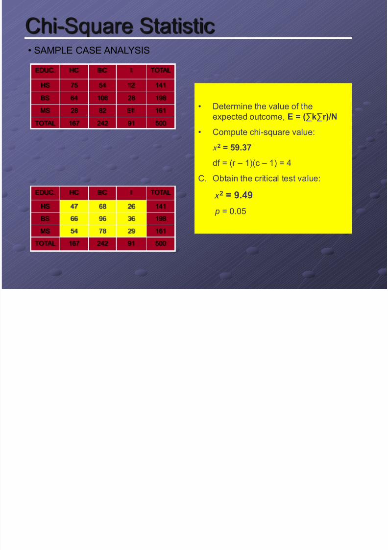
Chi-Square Statistic
EDUC. HC BC I TOTAL
HS 75 54 12 141
BS 64 106 28 198
MS 28 82 51 161
TOTAL 167 242 91 500
• SAMPLE CASE ANALYSIS
• Determine the value of the
expected outcome, E = (∑k∑r)/N
• Compute chi-square value:
x 2 = 59.37
df = (r – 1)(c – 1) = 4
C. Obtain the critical test value:
x 2 = 9.49
p = 0.05
EDUC. HC BC I TOTAL
HS 47 68 26 141
BS 66 96 36 198
MS 54 78 29 161
TOTAL 167 242 91 500

7/28/2019 Exploring Statistics
http://slidepdf.com/reader/full/exploring-statistics 32/33
Chi-Square Statistic• SAMPLE CASE ANALYSIS
• Decide whether the four groups really differ in opinionconcerning the components of a program toward crime
prevention.
PROGRAM Police LGU NGO Civilian TOTAL
Foot patrol 83 67 114 95 359
Motorized
patrol
37 33 86 55 211
TOTAL 120 100 200 150 570

7/28/2019 Exploring Statistics
http://slidepdf.com/reader/full/exploring-statistics 33/33
Chi-Square Statistic
Program P L N C TOTAL
Foot patrol 83 67 114 95 359
Motorized
patrol
37 33 86 55 211
TOTAL 120 100 200 150 570
• SAMPLE CASE ANALYSIS
• Determine the value of the
expected outcome, E = (∑k∑r)/N
• Compute chi-square value:
x 2 = 5.55
df = (r – 1)(c – 1) = 4
C. Obtain the critical test value:
x 2 = 7.82
p = 0.05
Program P L N C TOTAL
Foot patrol 76 63 126 94 359
Motorized
patrol
44 37 74 56 211
TOTAL 120 100 200 150 570