EXPLORING LOW-OXYGEN CONDITIONS IN THE CAMBRIAN …
202
EXPLORING LOW-OXYGEN CONDITIONS IN THE CAMBRIAN THROUGH TRILOBITES OF THE WHEELER SHALE by DOUGLAS L. JOHN (Under the Direction of Sally Walker) ABSTRACT The Middle Cambrian Wheeler Shale of Utah is host to one of the most famous trilobite assemblages in North America. These trilobites are exceptionally well- preserved, and many bear an unusually thick encrustation of cone-in-cone calcite. The conditions under which these trilobites lived and were preserved has been scrutinized in many previous studies; however, more detailed study has led only to more outstanding questions about the paleoenvironment in the Cambrian. The environment in the Wheeler Shale has been interpreted as dysoxic in the benthos, based on sedimentology and ichnofabric in the sediment, and on the occurrence of the benthic ptychopariid Elrathia kingii in low-diversity, high-abundance assemblages that are characteristic of such conditions in modern oceans. As a consequence of specialization for extreme low-oxygen conditions, Elrathia was proposed to be possibly symbiotic with sulfur-oxidizing bacteria, based on their morphological similarity to olenid trilobites. Olenids were previously proposed as symbiotic low-oxygen specialists, based on their morphology which would be well-suited to harboring symbionts.
Transcript of EXPLORING LOW-OXYGEN CONDITIONS IN THE CAMBRIAN …

EXPLORING LOW-OXYGEN CONDITIONS IN THE CAMBRIAN
THROUGH TRILOBITES OF THE WHEELER SHALE
by
DOUGLAS L. JOHN
(Under the Direction of Sally Walker)
ABSTRACT
The Middle Cambrian Wheeler Shale of Utah is host to one of the most famous
trilobite assemblages in North America. These trilobites are exceptionally well-
preserved, and many bear an unusually thick encrustation of cone-in-cone calcite. The
conditions under which these trilobites lived and were preserved has been scrutinized in
many previous studies; however, more detailed study has led only to more outstanding
questions about the paleoenvironment in the Cambrian.
The environment in the Wheeler Shale has been interpreted as dysoxic in the
benthos, based on sedimentology and ichnofabric in the sediment, and on the occurrence
of the benthic ptychopariid Elrathia kingii in low-diversity, high-abundance assemblages
that are characteristic of such conditions in modern oceans. As a consequence of
specialization for extreme low-oxygen conditions, Elrathia was proposed to be possibly
symbiotic with sulfur-oxidizing bacteria, based on their morphological similarity to
olenid trilobites. Olenids were previously proposed as symbiotic low-oxygen specialists,
based on their morphology which would be well-suited to harboring symbionts.

However, the accuracy of a symbiotic interpretation and the presence of low-oxygen
conditions that would predicate such symbiosis have not been directly examined.
This study addresses these questions by examining the morphological basis for
interpreting symbiosis in trilobites, and comparing putatively symbiotic forms to the
spectrum of morphologies among Cambrian trilobites. I search for direct evidence of
sulfur-oxidizing bacterial symbionts through molecular biomarkers associated with
trilobite exoskeletons. I perform several geochemical analyses that constrain the extent
and position of low-oxygen conditions above and below the sediment-water interface. I
found that symbiosis was not well supported in trilobites, and morphology may be related
more to taxonomic relationships than to environmental constraints such as reduced
oxygen. While biomarker evidence of bacterial symbionts was not found, fossils from
the Wheeler Shale revealed a suite of other biomarkers indicating more about
Anthropocene terrestrial changes, indicating fossils may be a storehouse for information
about modern ecosystem dynamics. Geochemistry suggests that benthic conditions were
not extremely dysoxic, and the distribution of Elrathia may not be related to
specialization for extreme low oxygen.
INDEX WORDS: Trilobite, Cambrian, Wheeler Shale, Symbiosis, Morphology,
Paleoenvironment, Biomarker, Anthropocene, Geochemistry,
Sulfur, Iron, Carbon, Trace metals, Dysoxia, Euxinia, Cone-in-
cone calcite, Taphonomy

EXPLORING LOW-OXYGEN CONDITIONS IN THE CAMBRIAN
THROUGH TRILOBITES OF THE WHEELER SHALE
by
DOUGLAS L. JOHN
B.S., The University of California at Riverside, 2004
M.S., The University of California at Riverside, 2008
A Dissertation submitted to the Graduate Faculty of the University of Georgia
In Partial Fulfillment of the Requirements for the Degree
DOCTOR OF PHILOSOPHY
ATHENS, GEORGIA
2016

© 2016
Douglas L. John
All Rights Reserved

EXPLORING LOW-OXYGEN CONDITIONS IN THE CAMBRIAN
THROUGH TRILOBITES OF THE WHEELER SHALE
By
DOUGLAS L. JOHN
Electronic Version Approved:
Suzanne Barbour
Dean of the Graduate School
The University of Georgia
May 2016
Major Professor: Sally Walker
Committee: Patricia Medeiros
Doug Crowe
Paul Schroeder
Alberto Perez-Huerta

iv
DEDICATION
To my wife Laura, whose love and support have kept me going through many a
long and stressful night of research and writing. Without her, this dissertation may never
have come to be.
And to my parents, for all their support throughout my educational career. It
brings me great satisfaction to know that I’ve done something worthy of the pride they
already feel for me.

v
ACKNOWLEDGEMENTS
I first thank my advisor, Sally Walker, for her endless support, encouragement, and
advisement throughout these studies. I extend my appreciation to the members of my
committee and the other faculty at the UGA Department of Geology for all their input
during this research project.
I also thank S. Holland for his advice on NMDS and H. D. Sheets for his advice on k-
means cluster analysis. West Desert Collectors and Jennifer Smith of Terra Trilobites of
Delta, UT provided assistance in acquiring samples and maintaining safe handling
protocols. Vancouver Petrographics of Vancouver, British Columbia prepared thin
sections. P. Medeiros and L. Babcock-Adams assisted with sample preparation and
biomarker analyses with GC-MS. The expertise of C. Fleisher and E. Formo in
performing the microprobe and ESEM analyses, respectively, is greatly appreciated.
Steve Bates at the Lyons Geochemistry Lab, University of California, Riverside,
provided training and assistance with geochemical analyses.
Funding for this research was provided by the Geological Society of America, the
Society for Sedimentary Geology (SEPM), the Watts-Wheeler Fund, and the National
Science Foundation (OCE-1057683).

vi
TABLE OF CONTENTS
Page
ACKNOWLEDGMENTS ............................................................................................v
CHAPTER
1 INTRODUCTION ................................................................................1
2 TESTING SYMBIOTIC MORPHOLOGY IN TRILOBITES UNDER
DYSOXIC AND OXIC CONDITIONS FROM CAMBRIAN TO EARLY
ORDOVICIAN LAGERSTÄTTEN ....................................................5
Introduction ...............................................................................7
Methods.....................................................................................11
Results .......................................................................................23
Discussion .................................................................................32
References .................................................................................40
Figures and Tables ....................................................................47
3 CAMBRIAN TRILOBITES AS ARCHIVES FOR ANTHROPOCENE
BIOMARKERS AND OTHER CHEMICAL COMPOUNDS ............67
Introduction ...............................................................................68
Methods.....................................................................................70
Results and Discussion .............................................................73
vii
Conclusion ................................................................................78
References .................................................................................79
Figures and Tables ....................................................................83
4 DIAGENESIS AND ELEMENTAL CHEMISTRY OF
EXCEPTIONALLY PRESERVED PUTATIVELY DYSOXIC
TRILOBITES FROM THE WHEELER SHALE.................................94
Introduction ...............................................................................96
Methods.....................................................................................100
Results .......................................................................................103
Discussion .................................................................................107
Conclusion ................................................................................113
References .................................................................................115
Figures and Tables ...................................................................119
5 CONSTRAINING OXYGEN AND SULFIDE LEVELS IN CAMBRIAN
WHEELER SHALE SEDIMENTS ......................................................136
Introduction ...............................................................................138
Methods.....................................................................................141
Results .......................................................................................147
Discussion .................................................................................150
Conclusion ................................................................................152
References .................................................................................153
Figures and Tables ...................................................................156
6 CONCLUSIONS...................................................................................163
viii
APPENDICES…
Appendix 2.1 .....................................................................................................165
Appendix 2.2 .....................................................................................................168
Appendix 2.3 .....................................................................................................170
Appendix 2.4 .....................................................................................................172
Appendix 3.1 .....................................................................................................177
Appendix 3.2 .....................................................................................................180
Appendix 4.1 .....................................................................................................184
Appendix 5.1 .....................................................................................................186
Appendix 5.2 .....................................................................................................187
Appendix 5.3 .....................................................................................................188
Appendix 5.4 .....................................................................................................189
Appendix 5.5 .....................................................................................................191
1
CHAPTER 1
INTRODUCTION
The Wheeler Shale of Utah contains one of the most well-known occurrences of
Cambrian (507 Ma) trilobites from North America. These trilobites are exceptionally
well-preserved, and unusually preserved in that they commonly occur with encrustations
of cone-in-cone calcite (CIC) up to several mm in thickness armoring their ventral
surfaces. Because of this unusual preservation, and because of their similarities to the
famous and roughly contemporaneous Burgess Shale, the Wheeler Shale has been well
studied; however, though over a century of scientific examination yielded a wealth of
data on the Wheeler Shale, much of it only raised further questions about the unique
conditions that generated the preservation of fossils discovered there.
The Wheeler Shale represents a mixed siliciclastic-carbonate environment,
restricted within a trough-bound basin in a shallow epeiric sea (Rees, 1986). The fossils
of the Wheeler Shale fall into three assemblages: a soft-bodied assemblage associated
with finely laminar sediments, thought to represent anoxic benthic conditions; a low-
diversity, high-abundance assemblage dominated by the ptychopariid trilobite Elrathia
kingii and species of the agnostid Peronopsis, associated with weakly laminar sediments
and thought to represent dysoxic conditions, and a more diverse benthic trilobite
assemblage associated with bioturbated sediments, interpreted as fully oxic conditions
(Gaines et al., 2005; Brett et al. 2009).

2
The unusual occurrence of Elrathia in these low-diversity assemblages, with only
the planktonic Peronopsis co-occurring, has been the focus of much attention: Gaines and
Droser (2003) interpreted them as low-oxygen specialists, the first benthic colonists
following the leading edge of the oxycline as it fell, based on the low-diversity, high-
abundance assemblages characteristic of modern animals with that mode of life, and on
the lack of pervasively bioturbated sediments where they were found. Gaines and Droser
(2003) also drew a parallel between Elrathia and the olenids of Fortey (2000), who
suggested that these trilobites were adapted for dysoxic or euxinic conditions through
symbiosis with sulfur-oxidizing bacteria. This hypothesis was based on the idea that an
olenimorph body plan – wide, flat, with numerous thoracic segments for harboring
symbionts, and a simple feeding structure – were particularly well-suited for such a mode
of life.
While the idea of symbiotic trilobites living in extreme environments is enticing,
there remains work to be done to ascertain if these conditions actually existed, and
whether trilobites actually carried out a symbiotic mode of life. Existing studies have
examined the ecology, sedimentology, and ichnofabric of the Wheeler Shale (Gaines and
Droser, 2003; Gaines et al., 2005; Brett et al., 2009), but aspects of the geochemistry
remain unexamined that could directly address the question of benthic oxygenation. The
question of symbiosis in trilobites, based thus far on morphology and occurrence, also
can be more rigorously examined, and direct evidence for symbiosis could be identified.
This study addresses these outstanding questions in four parts. In the first part, I
compare the characteristic morphology of putatively symbiotic trilobites with a group of
their contemporaries representing the broader range of Cambrian trilobite morphologies.

3
If symbiotic trilobites possessed a morphology uniquely suited for symbiosis, then they
should be morphologically distinct from the greater group of Cambrian trilobites, who
represented a great diversity of disparate life habits governing their own morphologies.
In the second part, I search for direct evidence of sulfur-oxidizing bacterial
symbionts through molecular biomarkers. If Elrathia had a symbiotic mode of life, then
biomarkers characteristic of those sulfur-oxidizing bacteria may be detected in
association with trilobite fossils.
In the third part, I compare the petrology and geochemistry of exoskeletal calcite
of Elrathia and Peronopsis. The presence of abundant cone-in-cone calcite in association
with exoskeletal calcite presents an opportunity to potentially compare geochemical
proxies representing seawater and porewater conditions. If Elrathia was living in low-
oxygen benthic conditions, and their skeletons still contain original calcite, then their
exoskeletons should bear a distinct geochemical signal from the oxic Peronopsis, and
from the later diagenetic calcites that formed in the sulfur-reduction zone necessary for
the formation of cone-in-cone structures. If both exoskeletons are similar to the
diagenetic calcites, then that suggests original exoskeletal calcite has been recrystallized
during diagenesis and reflects porewater conditions.
In the fourth part, I compare sulfur, iron, and trace metal proxies from the
sediment, to determine whether conditions on the seafloor were oxic, dysoxic, or euxinic,
and how extensive anoxia or euxinia was in the underlying sediments. If the seafloor was
not severely limited in oxygen, then some other factor than oxygenation may have been
driving the abundance patterns described in the Wheeler Shale. If the subsurface did not

4
have extensive bacterial sulfate reduction, then rapid formation of CIC could not have
occurred quickly after burial.

5
CHAPTER 2
TESTING SYMBIOTIC MORPHOLOGY IN TRILOBITES UNDER DYSOXIC AND
OXIC CONDITIONS FROM CAMBRIAN TO EARLY ORDOVICIAN
LAGERSTÄTTEN1
___________________________
1 John, D. L., and Walker, S. E. 2016. Testing symbiotic morphology in trilobites under
dysoxic and oxic conditions from Cambrian to Early Ordovician Lagerstätten.
Palaeogeography, Palaeoclimatology, Palaeoecology, 441, 704-720. Reprinted here with
permission of publisher.
6
Abstract
Dysoxic conditions were prevalent in Cambrian and Early Ordovician oceans.
Adaptations of trilobites to these conditions yield insight into the selective forces driving
their evolution and the potential for modern arthropods to adapt to anthropogenically-
driven dysoxia. In the early Paleozoic, olenid trilobites may have adapted to dysoxia
through olenimorphy, special morphologic adaptations facilitating symbiosis with sulfur-
oxidizing bacteria. Olenimorphy’s link to symbiosis has never been tested and might
instead be related to phylogeny. Here, we tested whether olenimorphy occurs
predominately in dysoxic environments, as expected, or whether it occurs within certain
trilobite groups regardless of environment. Trilobites were selected from nine fossil
Lagerstätten representing the early-to-middle Cambrian prior to olenid evolution and the
middle Cambrian-Early Ordovician Alum Shale with olenids, putative exemplars of
symbiosis. Trilobite morphology was scored as ranked characters and reduced via non-
metric multidimensional scaling (NMDS) to a single metric describing suitability for
symbiosis. Results indicated that olenimorphy was significantly related to phylogeny and
not environment. In the early-to-middle Cambrian, dysoxic corynexochids and oxic
redlichiids were equally unsuitable for symbiosis, while ptychopariids from both oxic and
dysoxic conditions were equally well-suited for symbiosis. In the Alum Shale, asaphids
and ptychopariids from both oxic and dysoxic conditions were equally well-suited for
symbiosis, and redlichiids from oxic conditions were poorly-suited. Olenids were not the
best-suited trilobites within their data set, nor even within their order. Secular trends in
thoracic segmentation did not bias our results. Trilobite hard parts do not appear to
provide evidence for symbiosis, which is consistent with modern arthropods that have

7
few morphological adaptations for dysoxic conditions. In fact, arthropods are rare in
persistently dysoxic conditions, raising concerns about the spread of anthropogenically-
triggered benthic dysoxia in the future, particularly given the extinction of trilobites
under similar conditions at the end of the Permian.
Introduction
Hypoxic conditions were prevalent in Cambrian and Early Ordovician oceans
when higher global temperatures, lower atmospheric O2, higher CO2 and continental
configurations contributed to stratified marine conditions in shallow shelf environments
(Frakes et al., 1992; Berner, 2006; Gill et al., 2011; Xu et al., 2012). Persistently hypoxic
conditions can lead to the development of dysoxia (critically low oxygen levels; < ~0.1
ml/l), as well as euxinia (low oxygen, free sulfate) where organic carbon input drives
microbial sulfate reduction generating H2S from ubiquitous oceanic sulfate (Canfield,
1989; Feng et al., 2014). For benthic environments, euxinia is typically achieved
whenever dysoxia persists beyond seasonal fluctuations and poor mixing generates a
well-stratified chemocline below oxic surface waters (e.g., the Black Sea, Nägler, 2011;
Slomp, 2013).
In modern oceans, persistently dysoxic environments such as oxygen minimum
zones (OMZs) are characterized by benthos adapted for dysoxia through, among other
factors, symbiosis with sulfur-oxidizing bacteria (Taylor and Glover, 2010). Dysoxic
environments are also characterized by low-diversity, high-abundance metazoan
assemblages (Levin et al., 2000). Modern benthic communities in persistently dysoxic
environments are dominated by polychaete worms, nematodes and bivalve mollusks,
8
while arthropods are not common (Lu and Wu, 2000; Levin, 2003; Sellanes et al., 2010).
In fact, modern arthropods show little tolerance for reduced oxygen conditions (Rabalais
et al., 2002; Vaquer-Sunyer and Duarte, 2008), though some arthropods have
morphological adaptations for high-sulfur conditions at hydrothermal vents such as
increased surface area of the mouthparts for cultivation of thiotropic symbionts (Petersen
et al., 2010).
It is curious, then, that at least some fossil arthropods – the trilobites – are
associated with dysoxic environments (Speyer and Brett, 1986; Lehmann et al., 1995;
Gaines and Droser, 2003). The mechanisms by which trilobites adapted to low-oxygen
conditions can elucidate the selective forces driving trilobite evolution and also shed light
on the potential for modern benthic arthropods to adapt to low oxygen levels that are
predicted to occur in the Anthropocene.
One group of trilobites thought to have adapted for low-oxygen conditions are the
late Cambrian to Ordovician olenids (Fortey and Owens, 1990). Fortey (2000) suggested
they adapted to reduced oxygen through symbiosis with sulfur-oxidizing bacteria. He
proposed a suite of morphological adaptations that would facilitate symbiosis, including
reduction in exoskeletal and muscular robustness spurred by reduced feeding and
predatory selective pressures, and a trend toward greater surface area under the
exoskeleton that would facilitate symbiont cultivation. Trilobites bearing these
morphologic characters, and thus similar to olenids, were termed olenimorphs (Fortey,
2000).
Fortey (2000) suggested that symbiosis, as indicated by olenimorph morphology,
may not be limited to the olenids and might be widespread among trilobites. For example,
9
Fortey’s morphological characters were used to suggest that the middle Cambrian
ptychopariid Elrathia kingii, from the mostly dysoxic Wheeler Shale, was possibly
symbiotic (Gaines and Droser, 2003). To date, Fortey’s morphological characters have
not been systematically tested to determine if they are indicative of symbiosis or are
simply a phylogenetic legacy of certain trilobite groups.
Here, we tested whether symbiotic morphology meets the expectation that it
occurs predominately in dysoxic environments or whether it occurs within particular
trilobite groups regardless of environment. Trilobites from nine fossil Lagerstätten,
representing the early Cambrian to Early Ordovician, were selected based on complete
taxonomic and environmental (sedimentology, geochemistry) descriptions. Fortey’s
qualitative morphological characters (i.e., thoracic segments, carapace morphology,
pleural morphology, hypostome attachment, and exoskeletal ornamentation) were
converted into ranked quantitative characters and scored for each genus, forming a
matrix. The matrix was then reduced via non-metric multidimensional scaling ordination
(NMDS) to a single metric that adequately synthesized the individual characters. This
metric described overall morphology for each trilobite as either well-suited for symbiosis,
yielding high NMDS scores, or poorly-suited for symbiosis, yielding low NMDS scores.
Two NMDS analyses were performed to examine the relationship of morphology with
phylogeny (i.e., different taxonomic groups) and environment (i.e., oxic versus dysoxic).
We first tested a set of early-to-middle Cambrian trilobites to describe the occurrence of
Fortey’s morphological characters prior to the evolution of olenids. One Ordovician
olenid, Hypermecaspis, a trilobite that Fortey (2000) deemed to be symbiotic, was
included to orient this analysis. Second, we tested a set of trilobites from the middle

10
Cambrian-Early Ordovician Alum Shale that included Fortey’s (2000) original olenids.
These trilobites represent a progression from an oxic, diverse assemblage in the middle
Cambrian to a dysoxic, olenid-dominated assemblage in the late Cambrian-Early
Ordovician.
A key issue that could affect our analyses is the fact that Cambrian trilobites had
greater variability in their thoracic segments and more segments overall than in later
periods (Hughes et al., 1999). Segmentation controls the number of gill structures, which
in turn increases surface area for symbiotic cultivation (Fortey 2000). This one character
could skew the NMDS scores of earlier trilobites artificially high, making them appear
more suitable for symbiosis. Therefore, we also tested the effect of segmentation on both
datasets to determine if segmentation was unduly affecting our analyses.
We predict that if Fortey’s morphological characters collectively describe adaptations for
symbiosis, then symbiotically-suitable trilobites (i.e., those with higher NMDS scores)
should be more common in dysoxic assemblages. A symbiotic life mode allows for
symbiotic trilobites to inhabit oxic waters, but not for oxic trilobites to inhabit dysoxic
waters (after Gaines and Droser, 2003).
The difference in morphology between olenimorphic and non-olenimorphic
trilobites should be even more pronounced in the later dataset (the Alum Shale) because
olenimorphy represents more primitive character states. For example, olenimorphic
trilobites have more segments, broad flat pleurae, unattached hypostome and a thin
exoskeleton, which are primitive characters (Fortey and Owens, 1990; Fortey, 2000).
Oxic trilobites should evolve away from these primitive character states given the
absence of selective pressures to retain that morphology (i.e., dysoxia). Thus, trilobites

11
from later periods should show a more distinct difference between oxic and dysoxic
morphologies, if olenimorphy is tied to symbiosis.
If the link between morphology and environment is confirmed, then symbiotic
trilobites can be identified in other assemblages. If this link is not confirmed, then
Fortey’s characters have a strong phylogenetic component, indicating that members of a
taxonomic group have similar morphologies regardless of environment.
Methods
Lagerstätten localities, assessment of relative oxygen levels and construction of datasets
We focused on fossil Lagerstätten that had well-preserved trilobites, complete
taxonomic descriptions, and adequate geochemical or sedimentary data that could be
binned into oxic and dysoxic environments. Both high and low diversity Lagerstätten
(suggestive of oxic and dysoxic assemblages, respectively) were considered if well
described.
Benthic conditions were not always persistently dysoxic, but could fluctuate
between dysoxic and oxic as oxyclines rose and fell (Gaines and Droser, 2003). While
some paleontological studies have discerned trilobite assemblages at bed-by-bed
resolution (e.g., Speyer and Brett, 1986, Gaines and Droser, 2003), most others do not
link trilobite occurrences with sedimentological or geochemical conditions at specific
horizons. Thus, a faunal list for a given locality may represent an amalgamation of
discrete oxic and dysoxic communities.
Because the majority of trilobites in our study could not be linked to specific
geochemical horizons, it was necessary to make assumptions about habitat based on the

12
general character of the Lagerstätten in which they occurred. Therefore, Lagerstätten
were classified as "mixed” or “mostly oxic” to describe their relative oxygen levels.
“Mixed” Lagerstätten contained regular intervals of dysoxic conditions as identified by
dark organic-rich sediment, sedimentary sulfide, lack of bioturbation, and/or
monospecific fossil horizons. Mixed localities were not exclusively dysoxic and
contained periodic oxic horizons, but can be generalized as more dysoxic relative to the
other Lagerstätten. “Mostly oxic” localities contained irregular intervals of dysoxia, or
had geochemical evidence that indicated that the water column was fully oxic above the
sediment-water interface. Euxinia was impossible to definitively ascertain for all
localities. An assumption was made that non-ephemeral periods of dysoxic deposition
would be accompanied by some euxinia at or just below the sediment-water interface,
which would allow sulfur-oxidizing bacterial symbionts to flourish.
Two datasets were constructed. The first dataset had trilobite taxa prior to olenid
evolution, representing eight Lagerstätten spanning the early-to-middle Cambrian from
sites worldwide (Fig. 2.1). Mostly oxic and mixed sites were each represented by four
Lagerstätten (Table 2.1, Appendix 2.1). The second dataset was constructed from the
Alum Shale Lagerstätte of Scandinavia, representing the middle Cambrian-Early
Ordovician. This locality, cited as an excellent example for studying evolutionary
processes (Clarkson and Taylor, 1995), contains the original olenids used to propose
symbiotic morphology (Fortey, 2000), as well as co-occurring non-olenids. The Alum
Shale has two distinct assemblages: a diverse middle Cambrian assemblage associated
with mostly oxic conditions and a late Cambrian-Early Ordovician olenid-dominated

13
assemblage associated with mixed conditions (Clarkson and Taylor, 1995 ; Appendix
2.2).
Selecting and classifying trilobite genera
Trilobites were selected for which all morphological characters could be
identified. The early-to-middle Cambrian dataset had 66 trilobite genera representing
three trilobite orders: 15 corynexochids (22.7%), 14 redlichiids (21.2%), and 37
ptychopariids (56.1%) (Appendix 2.1; see Symbiotic Character Matrix for descriptions of
morphological characters). The Ordovician olenid Hypermecaspis, an example from
Fortey (2000) of a symbiotically well-suited olenimorph, was added to the early-to-
middle Cambrian dataset to provide a point for comparison. Within the Alum Shale
dataset, 24 genera were identified including six asaphids (25%), three redlichiids
(12.5%), and 15 ptychopariids (62.5%), 11 of which were olenids (Appendix 2.2).
Ptychopariida and Redlichiida are considered paraphyletic groups, and the relationship of
the ptychopariids to post-Cambrian orders is not fully established (Lieberman and Karim,
2010). However, while widespread polyphyly has been suggested at the family level
within the ptychopariids (Cotton, 2001), the distinction between ptychopariids and non-
ptychopariids at the ordinal level is sufficient to recognize broad morphological
differences.
Trilobite genera were classified by environment as belonging to mostly oxic or
mixed sites (Table 2.1; Appendices 1-2). Because dysoxic trilobites could potentially
inhabit oxic waters, while oxic trilobites could not inhabit dysoxic waters, a trilobite was
considered “mixed” if it occurred within any mixed environment, or considered “mostly

14
oxic” if it occurred only within oxic environments. Within the early-to-middle Cambrian
dataset, 32 genera were classified as belonging to mixed and 34 to mostly oxic
environments, with Hypermecaspis also classified among the mixed trilobites. For the
Alum Shale, eight genera were from the mostly oxic middle Cambrian and 16 spanned
the mixed interval from the late Cambrian through the Early Ordovician.
The potential for under- and overrepresentation with respect to taxonomy
(ptychopariids versus non-ptychopariids) and environmental type (mixed versus mostly
oxic) was addressed for both datasets. No significant sample bias was detected in the
early-to-middle Cambrian dataset (Pearson’s chi-squared test: χ2 = 0.926, df = 1, and p =
0.336) or the Alum Shale dataset (Fisher’s exact test: p = 0.099). R was used for all
statistical tests (R Core Team, 2012), which were run at a significance level of α = 0.05,
except where otherwise stated.
Symbiotic character matrix
Fortey’s characters
Fortey’s (2000) descriptive characters for an ideal symbiotic trilobite include a
broad, flat, thin exoskeleton with abundant thoracic appendages, which would provide a
large surface area for symbiont cultivation. A symbiotic trilobite should also lack
complex feeding structures such as a carnivorous hypostome, because nutrition was
mostly derived from symbionts. Such a trilobite, like Hypermecaspis, would be
considered well-suited for symbiosis, whereas a trilobite without these characteristics
would be poorly-suited. Exoskeletal ornamentation was used as a substitute for carapace
thickness, because thickness could not be readily determined from published descriptions.

15
Fortey argued that a thick cuticle would have an unnecessary metabolic cost for a
symbiotic trilobite living in dysoxic conditions where predation was unlikely. Likewise,
an ornate exoskeleton would be unnecessary.
Character matrix: Character state rankings and normalization
Fortey’s descriptive characters were converted into five quantitative characters
with ranked character states (Table 2.2), producing a character matrix for the 66 early-to-
middle Cambrian genera plus Hypermecaspis and for the 24 Alum Shale genera. The
morphological characters for generic descriptions were drawn from the Paleobiology
Database (Landing et al., 2008) and the Treatise on Invertebrate Paleontology
(Harrington, 1959; Whittington et al., 1997). Genera for which all characters could not be
determined were not used in either dataset. All ranked character state values were
normalized to fall between 0 (least suitable for symbiosis) and 1 (most suitable), so that
all characters were equally weighted, as some characters were binary and others ternary.
A trilobite with character state values closer to 1 matched Fortey’s description for
symbiosis and has high symbiotic suitability, while a trilobite with character state values
closer to 0 does not, and has low symbiotic suitability. For example, Hypermecaspis
would have character state values of 1, indicating high suitability (Appendices 1-2).
NMDS analyses
NMDS for early-to-middle Cambrian and Alum Shale trilobites
The character matrix quantitatively describes the variation in morphology among
Fortey’s five characters across five dimensions. To simplify the character matrix to a

16
single dimension that describes overall symbiotic suitability for each trilobite, non-metric
multidimensional scaling (NMDS) was performed using Euclidean distance and the
metaMDS function of the R vegan library (Oksanen et al., 2013). As the data were
equally weighted for each character, Euclidean distance was an appropriate distance
measurement and should provide similar results to dissimilarity matrices such as Bray-
Curtis, which are less conservative as they do not satisfy triangle inequality (Anderson,
2006).
Twenty random starts were used to find the solution with the minimum stress.
Stress decreases substantially from one to two dimensions, and yields an acceptable level
of stress (Fig. 2.2; level of stress < 0.20; Rohlf 1970; Eallonardo and Leopold, 2014).
Therefore, a two-dimensional NMDS analysis was used to best reduce the data without
compromising its structure. The NMDS analysis generates an ordinated model that
describes the patterns within the dataset, and produces a metric that can be tested using
quantitative statistical methods. Comparison of these morphological data to independent
observations such as environmental and phylogenetic data can yield information about
the extrinsic factors potentially controlling morphology .
The major axis of the NMDS analysis (NMDS1) describes the majority of
variation within character state values, because variability in NMDS scores was greatest
along NMDS1 for both the early-to-middle Cambrian and Alum Shale datasets. If a
common factor such as phylogeny or environment is controlling suitability, NMDS1
scores would be a proxy for that factor’s effect. More positive NMDS1 scores indicate
trilobites more well-suited for symbiosis and more negative scores indicate trilobites
poorly-suited for symbiosis. For the early-to-middle Cambrian dataset, Hypermecaspis

17
should score high on NMDS1 and confirm that higher scores correspond to more
symbiotically-suitable morphologies. Likewise, Elrathia kingii, previously described as
potentially symbiotic, should also have high NMDS1 scores. Conversely, the redlichiid
Olenellus, whose spinose, tapering thorax and well-developed mouthparts would be
particularly maladapted for symbiotic cultivation and feeding, respectively, should score
low on NMDS1. For the Alum Shale, the olenids should score high on NMDS1. These
expectations would confirm the general effectiveness of NMDS for describing symbiotic
morphology.
Test for independence of characters in NMDS1 for early-to-middle Cambrian trilobites
Because symbiosis could affect all characters equally, if any character was more
strongly related to another character than to the NMDS axis, that would suggest those
characters were not sufficiently independent, and are describing much of the same
variation in the data, thus over-representing that variation. Therefore, a Spearman’s rank
correlation test was performed on each pairwise combination of characters and between
each character and NMDS1. Three of the ten pairwise relationships in the early-to-middle
Cambrian showed a significant correlation: segments with hypostome attachment and
exoskeletal ornamentation with both pleural morphology and hypostome attachment.
However, none of those relationships was stronger than the characters’ relationships to
NMDS1 (Table 2.3), and all characters were retained in the analysis.
If only some of the characters were influenced by environment, that might suggest
that those characters were being controlled by an environmental parameter other than
symbiosis. To test the strength of the relationship of each ranked character to

18
environmental conditions (mostly oxic or mixed), a Kruskal-Wallis rank-sum test was
performed for each character, and no significant relationships were found in the early-to-
middle Cambrian dataset, indicating none of the characters were strongly associated with
mostly oxic or mixed environments (Table 2.3).
Test for independence of characters in NMDS1 for Alum Shale trilobites
Similar to the early-to-middle Cambrian trilobites, pairwise relationships between
each character and between characters and NMDS1 were tested for the Alum Shale
trilobites using a Spearman’s rank correlation test. Within the Alum Shale, the only
significantly related characters were hypostome attachment and segmentation
(Spearman’s rho = -0.490, p = 0.02), and the only character not significantly correlated to
NMDS1 was segmentation (Table 2.3). Segmentation appears to be an anomalous
character in the Alum Shale, possibly driven by a trend in trilobites beginning in the late
Cambrian towards an overall reduction in number of segments; however, segmentation
does not appear to be introducing any significant bias on the overall NMDS analysis, and
thus was retained (see Testing for segmentation bias). All other characters were more
strongly correlated with NMDS1 than with any other character, indicating they were
adequately described by NMDS1. Exoskeletal ornamentation was not tested because all
trilobites in the Alum Shale had only one state, unornamented.
A Kruskal-Wallis rank-sum test revealed that hypostome attachment was
significantly related to environment (Table 2.3). This is likely because only redlichiids
had a conterminant hypostome, and redlichiids were exclusive to mostly oxic
environments. Because the control on hypostome attachment appears to be phylogenetic,
19
and because phylogeny is relevant to the analysis, hypostome attachment was retained in
the Alum Shale analysis.
Identifying morphologically distinct groups in NMDS
Plots of NMDS1 scores for all trilobites were generated for each of the five
characters. The score for each genus on NMDS1 and NMDS2 was given as a point. Each
genus was plotted with a symbol that corresponded to its character state and centroids for
each character were indicated with larger bold black symbols. The overall significant
correlation of character states to NMDS1 suggest that scores would be expected to
adequately express any patterns that might have existed within both datasets.
Because NMDS describes relative differences in morphology, any group of
morphologically distinct trilobites (such as symbiotic trilobites) should generate distinct
NMDS scores and plot similarly. To identify groups, k-means cluster analyses were
performed on NMDS scores for both datasets. The clusters were identified using 20
random starts of up to 100 iterations each. If clusters were identified, the utility of those
clusters for identifying distinct groups of symbiotically suitable trilobites was tested
against NMDS1 scores using one-sample t-tests. The 95% confidence intervals (95% CIs)
generated by the t-tests were used to define upper and lower NMDS1 thresholds, with
trilobites scoring above the upper threshold considered “moderately-suited" for
symbiosis. If any trilobites were identified as moderately-suited, another one-sample t-
test was done on that new group to identify trilobites scoring above that group’s 95% CI,
and those trilobites were considered “well-suited” for symbiosis. Because the data were
repartitioned for this second t-test, a new alpha level was used (α = 0.025) based on a
20
Bonferroni correction for multiple comparisons. Any cluster that contained entirely well-
suited trilobites was examined to determine if its members were from solely mixed
environments. If the trilobites were morphologically well-suited, but came from both
mostly oxic and mixed environments, then that would suggest they are not symbiotic,
because symbiosis is an adaptation specifically for low-oxygen conditions.
Testing for environmental and phylogenetic effects
Plots of overall NMDS1 scores for mostly oxic and mixed trilobite genera were
generated to examine whether trilobites from mixed localities had higher symbiotic
suitability. If NMDS1 describes suitability for symbiosis under more dysoxic conditions,
then trilobites from mixed localities should exhibit a higher average suitability than those
from mostly oxic localities. A two-sample t-test with a Welch correction was performed
to determine if the two environmental types were significantly different from each other.
The size of each sample (n = 34 mostly oxic, n = 33 mixed for early-to-middle Cambrian
trilobites; n = 8 mostly oxic, n = 16 mixed for Alum Shale trilobites) was sufficient for a
t-test (valid for n ≥ 5, de Winter, 2013). A non-parametric Wilcoxon rank sum test was
also performed, which confirmed the t-test results.
To assess whether there was any difference between mostly oxic and mixed
environments within each taxonomic order, NMDS scores for each trilobite order were
plotted separately, distinguishing between mixed and mostly oxic members. If mixed
trilobites had significantly higher NMDS1 scores than mostly oxic trilobites within any
one order, that might suggest symbiosis occurs only within that order. To gauge the
difference between mostly oxic and mixed members within each trilobite order, the
21
frequency distributions and average values of NMDS1 scores were plotted for genera
from each environment. The significance of those differences was assessed using a two-
sample t-test with a Welch correction and checked with a non-parametric Wilcoxon rank-
sum test. If the results from both tests were the same, only the t-test results were reported,
but if sample size was < 5, then Wilcoxon results were reported.
To test if phylogeny influenced NMDS scores, NMDS plots were generated for
each taxonomic order. If phylogeny is the main control on morphology, then NMDS
scores should be closer within each taxonomic order and farther apart between orders.
Testing for segmentation bias
Thoracic segmentation was more numerous and more variable in the early
evolution of trilobites (Hughes et al., 1999). Therefore, the number of segments for early
and middle Cambrian trilobites is expected to be greater than in later trilobites,
potentially inflating NMDS1 scores for the earlier groups and thereby potentially
increasing the number of seemingly symbiotic trilobites. Conversely, a reduction in
segments could skew the Alum Shale toward deflated NMDS1 scores and a decrease in
the apparent symbiotic suitability of later trilobites. We therefore did two tests to
determine if segmentation affected our analyses.
First, to determine if our data were affected by changes in the number of thoracic
segments, the mean and standard deviation for segment number was determined for each
taxonomic order from each of the three time periods (i.e., early Cambrian, middle
Cambrian, and late Cambrian-Early Ordovician) and for the combined assemblage from
each time period. If there was a trend towards reduced numbers of segments and reduced

22
variability in the number of segments, then the mean and standard deviations for the
number of segments should be lower by the late Cambrian-Early Ordovician. If such a
trend occurs, then its effects may be imparting a bias on the NMDS analyses for both
datasets. To determine the trend in segmentation for all trilobites across the three time
periods and test its significance, a generalized linear model (GLM) was fitted between
segmentation and time.
Second, to test how thoracic segmentation affected NMDS1 scores, the two
datasets were reduced in NMDS again without thoracic segmentation to generate a
second set of NMDS scores. The net shift in NMDS1 scores between the first and second
set of scores represents the overall direction of change, either positive or negative. This
was calculated in R as the sum of all positive and negative shifts in NMDS1 scores (i.e.,
NMDS1 scores without segmentation minus NMDS1 with segmentation for all genera in
each dataset). For the early-to-middle Cambrian dataset, if trilobites have more segments
overall and this is inflating NMDS scores, then removing segmentation should drive
overall NMDS1 scores lower. For the late Cambrian-Early Ordovician trilobites of the
Alum Shale, with putatively fewer segments, segmentation could potentially be deflating
NMDS scores. If so, removing segmentation should make NMDS1 scores increase for the
Alum Shale. The overall amount of change was determined through the mean absolute
shift in NMDS1 scores. This was calculated in R as the mean of the absolute difference in
NMDS scores for all genera in each dataset before and after segmentation was removed
from the analysis. A stronger effect of segmentation on NMDS scores would generate
larger shifts in both directions when segmentation was removed. If a secular reduction in
segmentation is biasing the analysis, then the effect of segmentation should be weaker in

23
the later Alum Shale dataset, when variability in segmentation is reduced and less of the
variation explained by NMDS is due to differences in segmentation. The significance of
the average change before and after removing segmentation was determined using a two-
sample t-test. If the distributions were not significantly different, this would suggest that
segmentation was not significantly biasing the analyses and that the NMDS analyses
were robust against any trend in segmentation.
Results
NMDS for early-to-middle Cambrian trilobites
Characters and morphologically-distinct groups generated by NMDS
In general, all five characters in the early-to-middle Cambrian trilobites became
monotonically more suitable along NMDS1 as scores increased (Fig. 2.3, refer to
centroids), indicating that all characters were adequately represented by NMDS1. The
number of thoracic segments increased from the least-suitable state to the most-suitable
state as scores increased (Fig. 2.3A). Carapace morphology also became more suitable
with greater NMDS1 scores, though arched and flat character states scored similarly (Fig.
2.3B). Pleural morphology (Fig. 2.3C), hypostome attachment (Fig. 2.3D) and
exoskeletal ornamentation (Fig. 2.3E) also increased in suitability with increased NMDS1
scores. The variations within each character along NMDS1 were all greater than along
NMDS2, indicating NMDS1 explained the majority of variation for each character.
Although possible, no individual character was described more strongly on NMDS2 than
on NMDS1.
24
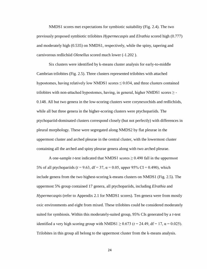
NMDS1 scores met expectations for symbiotic suitability (Fig. 2.4). The two
previously proposed symbiotic trilobites Hypermecaspis and Elrathia scored high (0.777)
and moderately high (0.535) on NMDS1, respectively, while the spiny, tapering and
carnivorous redlichiid Olenellus scored much lower (-1.202 ).
Six clusters were identified by k-means cluster analysis for early-to-middle
Cambrian trilobites (Fig. 2.5). Three clusters represented trilobites with attached
hypostomes, having relatively low NMDS1 scores ≤ 0.034, and three clusters contained
trilobites with non-attached hypostomes, having, in general, higher NMDS1 scores ≥ -
0.148. All but two genera in the low-scoring clusters were corynexochids and redlichiids,
while all but three genera in the higher-scoring clusters were ptychopariids. The
ptychopariid-dominated clusters correspond closely (but not perfectly) with differences in
pleural morphology. These were segregated along NMDS2 by flat pleurae in the
uppermost cluster and arched pleurae in the central cluster, with the lowermost cluster
containing all the arched and spiny pleurae genera along with two arched pleurae.
A one-sample t-test indicated that NMDS1 scores ≥ 0.490 fall in the uppermost
5% of all ptychopariids (t = 9.63, df = 37, α = 0.05, upper 95% CI = 0.490), which
include genera from the two highest-scoring k-means clusters on NMDS1 (Fig. 2.5). The
uppermost 5% group contained 17 genera, all ptychopariids, including Elrathia and
Hypermecaspis (refer to Appendix 2.1 for NMDS1 scores). Ten genera were from mostly
oxic environments and eight from mixed. These trilobites could be considered moderately
suited for symbiosis. Within this moderately-suited group, 95% CIs generated by a t-test
identified a very high scoring group with NMDS1 ≥ 0.673 (t = 24.49, df = 17, α = 0.025).
Trilobites in this group all belong to the uppermost cluster from the k-means analysis.

25
This group contained six genera including Hypermecaspis and could be considered well-
suited for symbiosis. If these ptychopariids occur within mixed environments, they meet
all expectations to be symbiotic. However, one of the five (i.e., Germaropyge) comes
from a mostly oxic locality; the other four from mixed. Segmentation bias could affect
the outcome of this early-to-middle Cambrian NMDS analysis, which we address in
Testing for segmentation bias in both datasets.
Environmental tests
Early-to-middle Cambrian trilobites were from an even mix of mostly oxic and
mixed environments, with centroids for both groups around zero on NMDS1 (Fig. 2.6A).
Both environmental groups were not significantly different from each other (t = 0.736, df
= 63.901, p = 0.465). Ptychopariids were evenly distributed between mostly oxic and
mixed assemblages with their centroids near 0.5 (Fig. 2.6B), and those environmental
groups were not significantly different from each other (t = 0.335, df = 29.123, p =
0.740). In contrast to ptychopariids, corynexochids and redlichiids were more
environment-specific and lower scoring. Most corynexochids were from mixed localities.
Corynexochids from mixed environments had a centroid near -0.5 that was lower than the
mostly oxic corynexochids with a centroid near zero. This was counter to expectations
that trilobites from mixed environments should have higher NMDS1 scores if
environment is controlling morphology (Fig. 2.6C). Importantly, corynexochid NMDS1
scores were not significantly different between environment groups (W = 5; p = 0.126).
In contrast to corynexochids, redlichiids occurred chiefly in mostly oxic localities. Their
NMDS1 scores for mostly oxic members were low, as expected, though scores for the

26
few mixed members were also low, with centroids both near -0.5 (Fig. 2.6D), and were
not significantly different (W = 3.5, p = 0.216).
Phylogenetic tests
There is a strong phylogenetic signal on NMDS1 scores for ptychopariid and non-
ptychopariid trilobites. All but three ptychopariid trilobites had positive NMDS1 scores,
while all but two each of corynexochids and redlichiids had negative scores (Fig. 2.7A).
NMDS1 scores for ptychopariids varied from slightly below average (i.e., zero) to
relatively high (Fig. 2.7B). Corynexochids and redlichiids scored lower than
ptychopariids, having very low to slightly above average NMDS1 scores (Fig. 2.7C-D).
Ptychopariid NMDS1 scores were significantly different from corynexochids (t = -6.416,
df = 16.846, p < 0.0001) and redlichiids (t = 7.3545, df = 16.005, p < 0.0001), indicating
ptychopariids were morphologically distinct from non-ptychopariids. However, there was
no significant difference between NMDS1 scores for corynexochids and redlichiids (t =
-0.411, df = 26.984, p = 0.684), indicating that low NMDS1 scores were associated with
non-ptychopariids in general.
NMDS for Alum Shale trilobites
Characters and morphologically-distinct groups generated by NMDS
For the Alum Shale trilobites, the five character states generally align uniformly
with NMDS1 scores: while one character is anomalous, three increase monotonically
with higher NMDS1 scores, and one has no comparative data (Fig. 2.8). Thoracic
segmentation did not increase monotonically, with a high number of segments
27
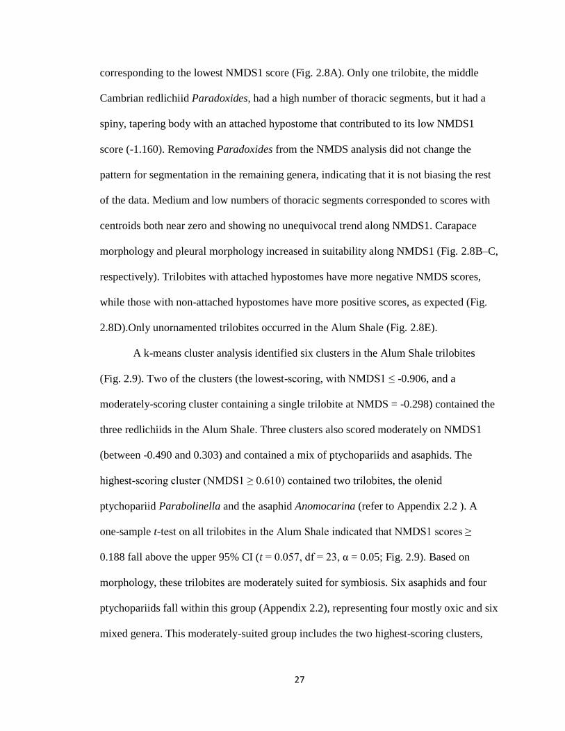
corresponding to the lowest NMDS1 score (Fig. 2.8A). Only one trilobite, the middle
Cambrian redlichiid Paradoxides, had a high number of thoracic segments, but it had a
spiny, tapering body with an attached hypostome that contributed to its low NMDS1
score (-1.160). Removing Paradoxides from the NMDS analysis did not change the
pattern for segmentation in the remaining genera, indicating that it is not biasing the rest
of the data. Medium and low numbers of thoracic segments corresponded to scores with
centroids both near zero and showing no unequivocal trend along NMDS1. Carapace
morphology and pleural morphology increased in suitability along NMDS1 (Fig. 2.8B–C,
respectively). Trilobites with attached hypostomes have more negative NMDS scores,
while those with non-attached hypostomes have more positive scores, as expected (Fig.
2.8D).Only unornamented trilobites occurred in the Alum Shale (Fig. 2.8E).
A k-means cluster analysis identified six clusters in the Alum Shale trilobites
(Fig. 2.9). Two of the clusters (the lowest-scoring, with NMDS1 ≤ -0.906, and a
moderately-scoring cluster containing a single trilobite at NMDS = -0.298) contained the
three redlichiids in the Alum Shale. Three clusters also scored moderately on NMDS1
(between -0.490 and 0.303) and contained a mix of ptychopariids and asaphids. The
highest-scoring cluster (NMDS1 ≥ 0.610) contained two trilobites, the olenid
ptychopariid Parabolinella and the asaphid Anomocarina (refer to Appendix 2.2 ). A
one-sample t-test on all trilobites in the Alum Shale indicated that NMDS1 scores ≥
0.188 fall above the upper 95% CI (t = 0.057, df = 23, α = 0.05; Fig. 2.9). Based on
morphology, these trilobites are moderately suited for symbiosis. Six asaphids and four
ptychopariids fall within this group (Appendix 2.2), representing four mostly oxic and six
mixed genera. This moderately-suited group includes the two highest-scoring clusters,

28
except for one genus that falls below the 95% CI, Agraulos (NMDS1 = 0.130). Another
one-sample t-test on the moderately-suited group indicated that NMDS1 scores ≥ 0.362
identified by the upper 95% CI could be considered a group well-suited for symbiosis (t =
8.552, df = 9, α = 0.025). This group contained two trilobites, Parabolinella and
Anomocarina, which correspond to the highest-scoring cluster. These trilobites represent
mostly oxic (Anomocarina) and mixed (Parabolinella) environments within the Alum
Shale, and therefore do not match expectations if symbiotic morphology is an adaptation
for dysoxic environments.
Environmental tests
Environment does not appear to have a strong influence on NMDS1 scores in the
Alum Shale. Trilobites from the middle Cambrian represent mostly oxic environments
yet have the lowest and highest NMDS1 scores within the Alum Shale and a centroid
slightly below zero (Fig. 2.10). The late Cambrian-Early Ordovician trilobites that
represent chiefly mixed environments overlap with the middle Cambrian trilobites, and
have moderately low to high NMDS1 scores with a centroid slightly above zero (Fig.
2.10). Importantly, centroids for mixed and mostly oxic genera were near zero and the
environmental groups were not significantly different from each other based on NMDS1
scores (t = 0.601, df = 8.605, p = 0.563).
Environment also does not exert a strong control over individual taxonomic
orders. NMDS1 centroids for mostly oxic and mixed ptychopariids were near zero and
the environmental groups were not significantly different from each other (Fig. 2.11A; t =
-1.870, df = 11.939, p = 0.086). The few mostly oxic ptychopariids actually had higher
29
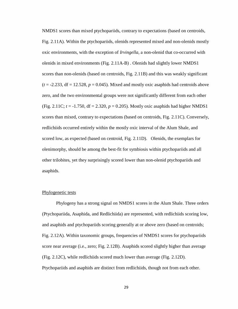
NMDS1 scores than mixed ptychopariids, contrary to expectations (based on centroids,
Fig. 2.11A). Within the ptychopariids, olenids represented mixed and non-olenids mostly
oxic environments, with the exception of Irvingella, a non-olenid that co-occurred with
olenids in mixed environments (Fig. 2.11A-B) . Olenids had slightly lower NMDS1
scores than non-olenids (based on centroids, Fig. 2.11B) and this was weakly significant
(t = -2.233, df = 12.528, p = 0.045). Mixed and mostly oxic asaphids had centroids above
zero, and the two environmental groups were not significantly different from each other
(Fig. 2.11C; t = -1.750, df = 2.320, p = 0.205). Mostly oxic asaphids had higher NMDS1
scores than mixed, contrary to expectations (based on centroids, Fig. 2.11C). Conversely,
redlichiids occurred entirely within the mostly oxic interval of the Alum Shale, and
scored low, as expected (based on centroid, Fig. 2.11D). Olenids, the exemplars for
olenimorphy, should be among the best-fit for symbiosis within ptychopariids and all
other trilobites, yet they surprisingly scored lower than non-olenid ptychopariids and
asaphids.
Phylogenetic tests
Phylogeny has a strong signal on NMDS1 scores in the Alum Shale. Three orders
(Ptychopariida, Asaphida, and Redlichiida) are represented, with redlichiids scoring low,
and asaphids and ptychopariids scoring generally at or above zero (based on centroids;
Fig. 2.12A). Within taxonomic groups, frequencies of NMDS1 scores for ptychopariids
score near average (i.e., zero; Fig. 2.12B). Asaphids scored slightly higher than average
(Fig. 2.12C), while redlichiids scored much lower than average (Fig. 2.12D).
Ptychopariids and asaphids are distinct from redlichiids, though not from each other.

30
Based on NMDS1 scores, ptychopariids were not significantly different from asaphids
(W = 28.5, p = 0.212), but were significantly different from redlichiids (W = 43, p =
0.018). Asaphids also had a significantly different distribution than redlichiids (W = 0, p
= 0.028 ).
Testing for segmentation bias in both datasets
Overall, there was little variation in the number of segments over time for both
datasets combined, with a mean of 12.38 segments in the early Cambrian, 12.37 segments
in the middle Cambrian, and 10.88 segments for the late Cambrian-Early Ordovician
(Table 2.4). The net change in the number of segments between the early Cambrian and
late Cambrian-Early Ordovician trilobites was 1.5 segments. However, standard
deviations increase from the early Cambrian to middle Cambrian, indicating increased
variability in segment number. This could be related to the higher taxonomic diversity in
the middle Cambrian datasets, where all four orders are represented. By the late
Cambrian-Early Ordovician, the total mean and standard deviation for the number of
segments was slightly lower than in the early Cambrian (Table 2.4).
Within groups, there was also little difference in the number of segments between
time periods (Table 2.4). Only three groups (i.e., the ptychopariids, redlichiids, and
asaphids) appear in more than one time period across both datasets to make meaningful
comparisons for trends in thoracic segmentation. Mean thoracic segmentation in
ptychopariids increased slightly from the early Cambrian (12.67) to the middle Cambrian
(13.83) and then decreased in late Cambrian-Early Ordovician (11.50). The standard
deviation for number of thoracic segments in ptychopariids rises from the early Cambrian
31
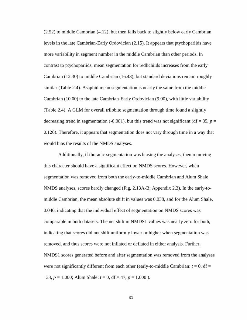
(2.52) to middle Cambrian (4.12), but then falls back to slightly below early Cambrian
levels in the late Cambrian-Early Ordovician (2.15). It appears that ptychopariids have
more variability in segment number in the middle Cambrian than other periods. In
contrast to ptychopariids, mean segmentation for redlichiids increases from the early
Cambrian (12.30) to middle Cambrian (16.43), but standard deviations remain roughly
similar (Table 2.4). Asaphid mean segmentation is nearly the same from the middle
Cambrian (10.00) to the late Cambrian-Early Ordovician (9.00), with little variability
(Table 2.4). A GLM for overall trilobite segmentation through time found a slightly
decreasing trend in segmentation (-0.081), but this trend was not significant (df = 85, p =
0.126). Therefore, it appears that segmentation does not vary through time in a way that
would bias the results of the NMDS analyses.
Additionally, if thoracic segmentation was biasing the analyses, then removing
this character should have a significant effect on NMDS scores. However, when
segmentation was removed from both the early-to-middle Cambrian and Alum Shale
NMDS analyses, scores hardly changed (Fig. 2.13A-B; Appendix 2.3). In the early-to-
middle Cambrian, the mean absolute shift in values was 0.038, and for the Alum Shale,
0.046, indicating that the individual effect of segmentation on NMDS scores was
comparable in both datasets. The net shift in NMDS1 values was nearly zero for both,
indicating that scores did not shift uniformly lower or higher when segmentation was
removed, and thus scores were not inflated or deflated in either analysis. Further,
NMDS1 scores generated before and after segmentation was removed from the analyses
were not significantly different from each other (early-to-middle Cambrian: t = 0, df =
133, p = 1.000; Alum Shale: t = 0, df = 47, p = 1.000 ).

32
Discussion
Testing Fortey’s symbiotic morphology using NMDS
Fortey (2000) suggested that olenimorphic trilobites had morphological
adaptations that facilitated symbiosis with sulfur-oxidizing bacteria as a response to
living in low-oxygen conditions. Dysoxic conditions were prevalent through the
Cambrian and Early Ordovician period, which would have created dysoxic and euxinic
conditions (herein referred to as mixed environments) for symbiotic trilobites to thrive
within. We tested Fortey’s morphological characters using NMDS to determine if
symbiotic morphology was indicative of trilobites living in mixed environments or was a
phylogenetic signal and not related to adaptation to environmental conditions. Character
states that are indicative of symbiotic morphology in trilobites as described by Fortey
(collectively referred to as olenimorphy) were synthesized into a single numerical metric,
NMDS1, using data from two sets of trilobites, with and without olenids. Higher scores
on NMDS1 would indicate overall greater symbiotic suitability: moderately high scores
represent moderately-suited trilobites, while distinctly high scores represent well-suited
trilobites.
We found that NMDS1 was a robust proxy that could describe overall suitability
for symbiosis in trilobites. In the early-to-middle Cambrian, individual character
suitability for symbiosis increased with higher values on NMDS1. The characters mostly
varied independently of each other, and every character was more closely correlated to
NMDS1 than to any other characters. This increase in suitability, however, does not mean
that symbiosis is controlling the distribution along NMDS1, as we discuss below.

33
In the Alum Shale, three of the five characters increased with higher values on
NMDS1. The two exceptions were exoskeletal ornamentation, which had only one state
represented, and segmentation, which had no trend in either direction along NMDS1
except for one outlier, Paradoxides, with a low NMDS1 score. However, the individual
effects of segmentation on the Alum Shale were small (see discussion on Segmentation)
and the inclusion of segmentation did not bias the analysis against the other characters.
The remaining three characters in the Alum Shale had low pairwise correlations, and
varied independently.
The independence of most characters in both datasets and their overall correlation
with the NMDS1 metric suggested that there was a common factor connecting the
characters that determined overall symbiotic suitability. Therefore, NMDS1 did not
appear to be simply modeling statistical noise and random variation. NMDS1 scores, as a
proxy for overall symbiotic suitability, were compared to environmental occurrence and
phylogenetic affinity. This served to determine the relative effects of environment and
phylogeny as common factors driving symbiotic morphology.
Identifying groups
Cluster and confidence interval analysis within both datasets failed to identify a
clear group of trilobites from exclusively mixed environments with significantly higher
NMDS1 scores, as would be expected if there was a population of morphologically-
distinct symbiotic trilobites that tracked dysoxic conditions. In the early-to-middle
Cambrian dataset, five high-NMDS1 scoring ptychopariids could potentially be
symbiotic, but one of those five represented an oxic environment, suggesting that the
34
common factor governing their distinct morphology was not likely environmentally
driven. Moderately-suited trilobites also represented a mix of mostly oxic and mixed
environments in the early-to-middle Cambrian. In the Alum Shale, two well-suited
trilobites were identified, an asaphid and a ptychopariid, but they represented mostly oxic
and mixed environments, respectively. Moderately-suited trilobites in the Alum Shale
were not exclusively dysoxic either.
Olenimorphy does not appear to describe a special adaptation for symbiosis.
Symbiosis itself is a binary character: organisms either are symbiotic or are not, and
morphologies dependent on symbiosis would be expected to show a binary pattern as
well, which should be manifest in the NMDS1 scores for trilobites. The 95% CI analysis
does not support this, with neither well-suited nor moderately-suited groups in either
dataset showing a dominance of mixed genera. Overall symbiotic suitability appears
continuous from “less olenimorphic” to “more olenimorphic”, rather than showing a
distinction between discrete “symbiotic” and “non-symbiotic” morphologies, which
strongly indicates a phylogenetic influence, rather than an environmental adaptation, for
so-called symbiotic morphology.
Environment
Environment did not appear to exert an influence on morphology at any point in
the analyses. No individual character was significantly correlated to environmental
conditions in both data sets, suggesting even before any NMDS results that an
environmental control on morphology was unlikely. For the early-to-middle Cambrian,
redlichiids from mostly oxic environments and corynexochids from mixed environments

35
scored similarly low on NMDS1, suggesting environment was not driving any difference
in their morphologies, while ptychopariids representing both environments scored
uniformly higher than the other orders. Redlichiids in the Alum Shale, represented by
mostly oxic environments, scored low on NMDS1, as expected. However, asaphids and
ptychopariids from mixed environments scored similarly to their counterparts in mostly
oxic environments, counter to expectations. The lack of any distinct environmental
gradient in NMDS1 scores indicates that environment (i.e., mostly oxic vs. mixed) is not
a major factor driving changes in trilobite morphology.
The difference in morphology between oxic and dysoxic assemblages should
increase through time, because the character states associated with olenimorphy are
primitive states for those characters. Therefore, trilobites would evolve towards
progressively more derived (i.e., less olenimorphic) character states, in the absence of a
factor such as symbiosis favoring retention of the primitive states. However, no
difference in NMDS1 scores between oxic and dysoxic assemblages was detected in
either data set, suggesting symbiosis was not driving changes in morphology.
It is worth nothing that, in the absence of a single common factor (i.e., symbiosis)
holistically controlling morphology, individual characters would be free to independently
respond to environment. For example, having a wide thorax with numerous thoracic
segments would increase gill surface area, thus improving suitability for dysoxic
conditions even without symbiosis. However, other features associated with symbiotic
morphology, such as a natant hypostome, would not affect dysoxic suitability. The lack
of a strong pairwise correlation between any one character and environmental conditions
indicates that environment is not a major factor governing morphology, even outside a
36
symbiotic hypothesis. This suggests that trilobite adaptive strategies for dysoxia did not
have a strong morphological component.
Phylogeny
Phylogeny appears to be the primary factor that controlled morphology, not
environmental pressure from dysoxic conditions. NMDS1 scores were primarily linked to
phylogenetic affiliation, irrespective of environment. In the early-to-middle Cambrian,
ptychopariids scored significantly higher than corynexochids and redlichiids on NMDS1,
regardless of environment. Corynexochids and redlichiid NMDS1 scores were not
significantly different from each other, despite strong environmental differences. In the
Alum Shale, asaphids and ptychopariids scored significantly higher than redlichiids, but
they were not significantly different from each other. Asaphids are descended from
ptychopariids (Fortey and Chatterton, 1988), suggesting that their phylogenetic similarity
is expressed in similar NMDS scores. In general, asaphids score higher than
ptychopariids, and olenids in particular, despite occurring in mostly oxic and mixed
intervals in the Alum Shale. The asaphids indicated that morphological characters
interpreted as symbiotic (i.e., a broad flat thorax with flat, wide pleurae and numerous
thoracic segments) can be expressed even more strongly in non-olenids than in the
olenids themselves, including in trilobites from mostly oxic environments. While olenids
(representing mixed environments) were distinct from non-olenid ptychopariids
(representing mostly oxic environments), the non-olenid ptychopariids scored higher,
contrary to expectations. Thus, it appears that olenimorphy is much more strongly related
to phylogeny than environment.
37
Segmentation
The number of thoracic segments is one of the characters incorporated into
NMDS1 scores. Because Lower Paleozoic trilobites have an evolutionary trend toward a
decrease in thoracic segmentation over time, this character could bias our analyses and
recognition of putatively symbiotic trilobites. Hughes et al. (1999) suggested that
variability in segmentation was highest during the Cambrian, and then stabilized toward a
decrease in average segmentation in later periods. Therefore, more symbiotically suitable
trilobites could be identified in the early-to-middle Cambrian dataset than in the Alum
Shale if this trend in the number of segments was affecting the outcome of our analyses.
However, when trilobites from both datasets were compared to time, overall number and
variability of thoracic segments did not show any trends, though ptychopariids did have
higher variability in the number of thoracic segments in the middle Cambrian, in
accordance with the findings of Hughes et al. (1999). The GLM likewise found only a
small and non-significant decrease in segmentation through time.
Segmentation did not bias the outcome of the NMDS analyses. When
segmentation was removed from both data sets, NMDS1 scores shifted minimally, but in
no particular direction, and the shifts were not significant. Removal of segmentation did
not shift NMDS1 scores lower in the early-to-middle Cambrian trilobites or higher for the
Alum Shale trilobites, as expected if segmentation was artificially inflating or deflating
NMDS1 scores. Therefore, segmentation did not have a disproportionately strong
influence on overall NMDS scores in either dataset, which validates the inclusion of
segmentation in the analyses.

38
Implications for modern arthropods
Based on our analyses, trilobites demonstrated low morphological response to
environmental change, which raises the question of how modern arthropods might cope
with the loss of suitable habitat as dysoxia potentially spreads in warming oceans. It is
possible that trilobites adapted physiologically without major morphological change,
which could explain why some trilobites are found in dysoxic conditions despite their
morphological similarity to more oxic genera.
In modern icehouse oceans, dysoxia occurs intermittently with seasonal blooms of
phytoplankton and eutrophication, or more permanently over nutrient-upwelling zones
(Diaz, 2001). These dysoxic areas are limited in size, because robust deep-water
circulation promotes thorough mixing of oxygenated waters (Toggweiler and Russell,
2008). Modern fauna have adapted to avoid dysoxic waters and to quickly recolonize the
benthos after reoxygenation, rather than persevere through intermittent dysoxia (Lu and
Wu, 2000). In contrast, hothouse dysoxic conditions, like those in the Cambrian, are
larger and more prolonged because the circulation and solubility of oxygen in the oceans
decreases with increased temperature (Slomp, 2013). In particular, fossil arthropods in
persistently dysoxic conditions that were not able to migrate to more oxic waters went
extinct (Williams et al., 2011). Arthropods appear inherently poorly-suited to adapt to
persistent dysoxia. An increase in persistently dysoxic zones could occur over the next
century, as global ocean circulation weakens and oxygen solubility decreases with rising
global temperatures, which does not bode well for marine arthropods.
Such a prolonged change in oxygenation would represent a new challenge for
modern arthropods. Symbiotic arthropods are not a major part of modern dysoxic
39
communities (Levin, 2003), making symbiosis an unlikely adaptation. Where they do
occur, modern symbiotic arthropods do not significantly modify their hard parts. For
example, chemosynthetically symbiotic shrimp at sulfur-rich vents only modify the
internal surface of their mouthparts for cultivation of symbionts (Petersen et al., 2010),
suggesting low morphological flexibility similar to trilobites. Furthermore, it is unlikely
that trilobites shared symbiosis as a common behavior at the family level (i.e., olenids) or
higher (i.e., olenimorphs). Where modern arthropod ectosymbiotic relationships do occur,
they tend to occur at the generic level, with different symbiotic assemblages associated
with different genera of hosts (Ott et al., 2004). The variety of symbiotic relationships
suggests that symbiosis is a highly-derived evolutionary behavior tied to specific, and
perhaps, extreme environments like deep-sea hydrothermal vents, and not deeply intrinsic
to any group of arthropod. If symbiosis did occur, it may have been ectosymbiosis, which
is not easy to identify purely from hard part morphology.
The lack of adaptive responses to dysoxia for arthropods, aside from migration,
raises the possibility for significant faunal turnover in the Anthropocene. Arthropod
species could become extirpated from growing dysoxic environments because they are
unable to adapt, even under relatively mild dysoxia. An analogue for future oceans might
be the final extinction of trilobites at the end-Permian, which has been associated with a
global spread of persistent dysoxic to euxinic environments, linked at least partially to
global warming (Bond and Wignall, 2010; Liao et al., 2010). Given the economic
importance of many benthic arthropods as food stocks, and their ecological importance as
predators and scavengers, this could lead to noticeable effects on human and
environmental sustainability.

40
References
Anderson, M. J., 2006. Distance-based tests for homogeneity of multivariate dispersions.
Biometrics, 62(1), 245-253.
Berner, R.A., 2006. GEOCARBSULF: A combined model for Phanerozoic atmospheric
O2 and CO2. Geochimica et Cosmochimica Acta, 70, 5653-5664.
Bond, D.P., Wignall, P.B., 2010. Pyrite framboid study of marine Permian–Triassic
boundary sections: a complex anoxic event and its relationship to contemporaneous
mass extinction. Geological Society of America Bulletin, 122(7-8), 1265-1279.
Brett, C.E., Allison, P.A., DeSantis, M.K., Liddell, W.D., Kramer, A., 2009. Sequence
stratigraphy, cyclic facies, and lagerstätten in the Middle Cambrian Wheeler and
Marjum Formations, Great Basin, Utah. Palaeogeography, Palaeoclimatology,
Palaeoecology, 277, 9-33.
Canfield, D.E. 1989. Sulfate reduction and oxic respiration in marine sediments:
implications for organic carbon preservation in euxinic environments. Deep Sea
Research Part A. Oceanographic Research Papers, 36(1), 121-138.
Caron, J., Jackson, D, 2008. Paleoecology of the Greater Phyllopod Bed community,
Burgess Shale. Paleogeography, Paleoclimatology, Paleoecology, 258, 222-256.
Chlupac, I., Kordule, V., 2002. Arthropods of Burgess Shale type from the Middle
Cambrian of Bohemia (Czech Republic). Bulletin of the Czech Geologic Survey,
77(3), 167-182.
Clarkson, E.N.K., Taylor, C. M., 1995. The lost world of the olenid trilobites. Geology
Today, 11(4), 147-154.

41
Conway Morris, S., 1986. The community structure of the Middle Cambrian phyllopod
bed (Burgess Shale). Paleontology, 29, 423-467.
Cotton, T.J., 2001. The phylogeny and systematics of blind Cambrian ptychoparioid
trilobites. Palaeontology, 44(1), 167-207.
De Winter, J.C.F., 2013. Using the Student’s t-test with extremely small sample sizes.
Practical Assessment, Research & Evaluation, 18(10), 1-12.
Diaz, R.J., 2001. Overview of hypoxia around the world. Journal of Environmental
Quality, 30(2), 275-281.
Eallonardo Jr., A.S., Leopold, D.J., 2014. Inland salt marshes of the northeastern United
States: stress, disturbance, and compositional stability. Wetlands, 34(1), 155-166.
Fatka, O., Kordule, V., Szabad, M., 2004. Stratigraphical distribution of Cambrian fossils
in the Pribram-Jince Basin (Barrandian area, Czech Republic). Senckenbergiana
Lethaea, 84, 367-381.
Feng, L., Li, C., Huang, J., Chang, H., Chu, X., 2014. A sulfate control on marine mid-
depth euxinia on the early Cambrian (ca. 529-521 Ma) Yangtze platform, South
China. Precambrian Research, 246, 123-133.
Fortey, R., 2000. Olenid trilobites: The oldest known chemoautotrophic symbionts?
Proceedings of the National Academy of Sciences, 97, 6574-6578.
Fortey, R. A. Chatterton, B. D. E., 1988. Classification of the Trilobite Suborder
Asaphina. Palaeontology 31(1), 165-222.
Fortey, R., Owens, R.M., 1990. Trilobites. Pp. 121-142 in K.J. McNamara, ed.
Evolutionary trends. University of Arizona Press, Tucson.

42
Frakes, L.A., Francis, J.E., Syktus, J.I., 1992. Climate modes of the Phanerozoic.
Cambridge University Press, 288 pp.
Gaines, R.R., Droser, M. L., 2003. Paleoecology of the familiar trilobite Elrathia kingii:
an early exaerobic zone inhabitant. Geology, 31, 941-944.
Gaines, R.R., Droser, M.L., 2010. The paleoredox setting of Burgess Shale-type deposits.
Palaeogeography, Palaeoclimatology, Palaeoecology, 297, 649-661.
Garson, D.E., Gaines, R.R., Droser, M.L., Liddell, W.D., Sappenfield, A., 2012.
Dynamic palaeoredox and exceptional preservation in the Cambrian Spence Shale of
Utah. Lethaia, 45(2), 164-177.
Gehling, J.G., Jago, J.B., Paterson, J.R., García-Bellido, D.C., Edgecombe, G.D., 2011.
The geological context of the lower Cambrian (Series 2) Emu Bay Shale Lagerstätte
and adjacent stratigraphic units, Kangaroo Island, South Australia. Australian Journal
of Earth Sciences, 58(3), 243-257.
Gill, B.C., Lyons, T.W., Young, S.A., Kump, L.R., Knoll, A.H., Saltzman, M.R., 2011.
Geochemical evidence for widespread euxinia in the Later Cambrian ocean. Nature,
469, 80-83.
Harrington, H.J, 1959. Systematic Descriptions. Pp. O170-O590 in Part O – Arthropoda 1
of R.C. Moore, ed. Treatise on invertebrate paleontology. Geological Society of
America, New York, and University of Kansas Press, Lawrence.
Hintze, L.F., and Robison, R.R., 1975. Middle Cambrian stratigraphy of the House, Wah
Wah, and Adjacent Ranges in Western Utah. Geological Society of America Bulletin,
86, 881-891.

43
Hughes, N. C., Chapman, R. E., and Adrain, J. M., 1999, The stability of thoracic
segmentation in trilobites: a case study in developmental and ecological constraints,
Evolution & Development, 1(1):24-35.
Landing, E., Johnson, S.C., Geyer, G., 2008. Faunas and Cambrian volcanism on the
Avalonian marginal platform, southern New Brunswick. Journal of Paleontology,
82(5), 884-905.
Lehmann, D., Brett, C.E., Cole, R., Baird, G., 1995. Distal sedimentation in a peripheral
foreland basin: Ordovician black shales and associated flysch of the western Taconic
foreland, New York State and Ontario. Geological Society of America Bulletin, 107,
708-724.
Levin, L.A., Gage, J.D., Martin, C., and Lamont, P.A., 2000. Macrobenthic community
structure within and beneath the oxygen minimum zone, NW Arabian Sea. Deep Sea
Research II, 47, 189-226.
Levin, L.A., 2003. Oxygen minimum zone benthos: adaptation and community response
to hypoxia. Oceanic and Marine Biology: an Annual Review, 41, 1-45.
Liao, W., Wang, Y., Kershaw, S., Weng, Z., Yang, H., 2010. Shallow-marine dysoxia
across the Permian–Triassic boundary: evidence from pyrite framboids in the
microbialite in South China. Sedimentary Geology, 232(1), 77-83.
Lieberman, B. S., and Karim, T. S., 2010. Tracing the trilobite tree from the root to the
tips: A model marriage of fossils and phylogeny. Arthropod Structure &
Development, 39, 111-123.
Lu, L., Wu, R.S.S., 2000. An experimental study on recolonization and succession of
marine macrobenthos in defaunated sediment. Marine Biology, 136, 291-302.

44
Nägler, T.F., Neubert, N., Böttcher, M.E., Dellwig, O., Schnetger, B., 2011.
Molybdenum isotope fractionation in pelagic euxinia: Evidence from the modern
Black and Baltic Seas. Chemical Geology, 289(1), 1-11.
Nedin, C., 1995. The Emu Bay Shale, a Lower Cambrian fossil Lagerstätte, Kangaroo
Island, South Australia. Memoirs of the Association of Australian Palaeontologists,
18, 31-40.
Oksanen, J., Blanchet, F.G., Kindt, R., Legendre, P., Minchin, P.R., O'Hara, R.B.,
Simpson, G.L., Solymos, P., Stevens, M.H.H., Wagner, H., 2013. Vegan: Community
Ecology Package, R package version 2.0-9. http://CRAN.R-
project.org/package=vegan.
Ott, J., Bright, M., Bulgheresi, S., 2004. Marine microbial thiotrophic ectosymbioses.
Oceanography and Marine Biology: An Annual Review, 42:95-118.
Palmer, A. R., Halley, R. B., 1979. Physical stratigraphy and trilobite biostratigraphy of
the Carrara Formation (Lower and Middle Cambrian) in the southern Great Basin
(No. 1047). US Govt. Printing Office.
Petersen, J.M., Ramette, A., Lott, C., Cambon-Bonavita, M.A., Zbinden, M., Dubilier,
N., 2010. Dual symbiosis of the vent shrimp Rimicaris exoculata with filamentous
gamma- and epsilonproteobacteria at four Mid-Atlantic Ridge hydrothermal vent
fields. Environmental Microbiology, 12, 2204-2218.
R Core Team, 2012. R: A language and environment for statistical computing. R
Foundation for Statistical Computing, Vienna, Austria, http://www.R-project.org/.
Rabalais, N.N., Turner, R.E., Wiseman, Jr., W.J., 2002. Gulf of Mexico Hypoxia, AKA
"The Dead Zone". Annual Review of Ecology and Systematics, 33, 235-263.

45
Retallack, G., 2011. Exceptional fossil preservation during CO2 greenhouse crises?
Paleogeography, Paleoclimatology, Paleoecology, 307, 59-74.
Rohlf, F.J., 1970. Adaptive hierarchical clustering schemes. Systematic Zoology, 18, 58-
82.
Sellanes, J., Neira, C., Quiroga, E.. Teixido, N., 2010. Diversity patterns along and across
the Chilean margin: a continental slope encompassing oxygen gradients and methane
seep benthic habitats. Marine Ecology, 31(1), 111-124.
Shu, D., Vannier, J., Luo, H., Chen, L., Zhang, X., Hu, S., 1999. Anatomy and lifestyle of
Kunmingella (Arthropoda, Bradoriida) from the Chengjiang fossil Lagerstätte (lower
Cambrian; southwest China). Lethaia, 32(4), 279-298.
Slomp, C.P., 2013. Reconstructing the history of euxinia in a coastal sea. Geology, 41,
523-524.
Speyer, S.E., Brett, C.E., 1986. Trilobite taphonomy and Middle Devonian taphofacies.
Palaios, 1(3), 312-327.
Steiner, M., Zhu, M.Y., Weber, B., Geyer, G., 2001. The Lower Cambrian of eastern
Yunnan: trilobite-based biostratigraphy and related faunas. Acta Palaeontologica
Sinica, 40(suppl.), 63-79.
Taylor, J.D., Glover, E.A., 2010. Chemosymbiotic bivalves. Pp. 107-135, in The vent and
seep biota. Springer Netherlands.
Toggweiler, J.R., Russell, J., 2008. Ocean circulation in a warming climate. Nature,
451(7176), 286-288.
Vaquer-Sunyer, R., Duarte, C.M., 2008. Thresholds of hypoxia for marine biodiversity.
Proceedings of the National Academy of Sciences, 105, 15452-15457.

46
Webster, M., Sadler, P.M., Kooser, M.A., Fowler, E., 2008. Combining stratigraphic
sections and museum collections to increase biostratigraphic resolution. Pp. 95-128 in
P.J. Harries, ed. High-Resolution Approaches in Stratigraphic Paleontology. Springer
Netherlands.
Whittington, H.B., Chatterton, B.D.E., Speyer, S.E., Fortey, R.A., Owens, R.M., Chang,
W.T., Dean, W.T., Jell, P.A., Laurie, J.R., Palmer, A.R., Repina, L.N., Rushton,
A.W.A., Shergold, J.H., Clarkson, E.N.K., Wilmot, N.V., Kelly, S.R.A., 1997. Part
O, Revised. Arthropoda 1: Trilobita: Introduction, order Agnostida and order
Redlichiida. in R.L. Kaesler, ed. Treatise on invertebrate paleontology. Geological
Society of America, Boulder, Co., and University of Kansas Press, Lawrence, 530 pp.
Williams, M., Vannier, J., Corbari, L., Massabau, J.C., 2011. Oxygen as a driver of early
arthropod micro-benthos evolution. PLoS ONE, 6(12), e28183.
Xu, L., Lehmann, B., Mao, J., Nägler, T.F., Neubert, N., Böttcher, M.E., Escher, P.,
2012. Mo isotope and trace element patterns of Lower Cambrian black shales in
South China: Multi-proxy constraints on the paleoenvironment. Chemical Geology,
318, 45-59.
Zhao, F., Caron, J.B., Hu, S., Zhu, M., 2009. Quantitative analysis of taphofacies and
paleocommunities in the Early Cambrian Chengjiang Lagerstätte. Palaios, 24(12),
826-839.

47
Figures and Tables
Fig. 2.1. Map of localities for Cambrian paleogeography. From west to east: A,
Chengjiang. B, Latham and Spence Shales. C, Wheeler and Marjum Shales. D, Burgess
Shale. E, Jince. F, Emu Bay. Map modified from Ron Blakey, NAU Geology, early
Cambrian paleogeography.
Fig. 2.2. Stress of NMDS model from one to four dimensions for the early-to-middle
Cambrian dataset. A two-dimensional model best describes the variation in the character
matrix (i.e., stress below 0.2) while minimizing dimensions. The model was iterated 20
times to achieve the best solution, but reached a minimum after ten.

48
Fig. 2.3. Results of NMDS for trilobites of the early-to-middle Cambrian, including
Hypermecaspis, symbolically coded by character state. Centroids for each character state
are coded with bold black symbols. Higher positive scores on NMDS1 correspond to
greater symbiotic suitability. A, Character states for number of segments, with a trend
toward higher number of segments asNMDS1 scores increase. B, Carapace morphology
increases along with NMDS1 scores from highly arched through arched to flat
morphologies. C, Pleural morphology, with a trend toward flatter pleurae with increased
NMDS1 scores. D, Hypostome attachment has two distinct groupings: non-attached
hypostomes correspond to higher NMDS1 scores, attached hypostomes to lower scores.
E, Exoskeletal ornamentation has two groups, with ornamented trilobites scoring lower
onNMDS1 than non-ornamented trilobites. Ornamented trilobites were
the lowest-scoring on NMDS1 of all character-state groups.
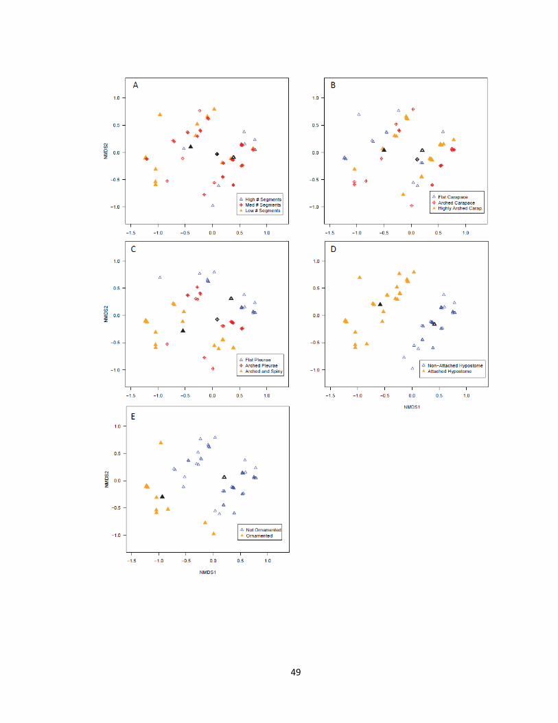
49
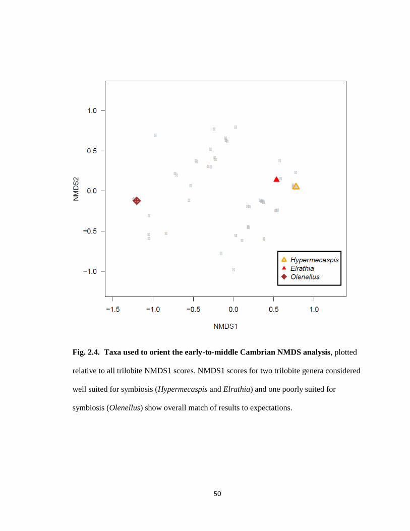
50
Fig. 2.4. Taxa used to orient the early-to-middle Cambrian NMDS analysis, plotted
relative to all trilobite NMDS1 scores. NMDS1 scores for two trilobite genera considered
well suited for symbiosis (Hypermecaspis and Elrathia) and one poorly suited for
symbiosis (Olenellus) show overall match of results to expectations.

51
Fig. 2.5. K-means cluster analysis for NMDS scores for trilobites from the early-to-
middle Cambrian. Six clusters were identified (see text). Upper cutoff thresholds for
95% confidence intervals from single-sample t-tests of ptychopariids are indicated with
dashed lines. NMDS1 scores above 0.490 (left dashed line) represent potentially
moderately suited genera; scores above 0.673 (right dashed line) represent potentially
well-suited genera.

52
Fig. 2.6. Results of NMDS for mixed and mostly oxic genera in the early-to-middle
Cambrian, sorted by taxonomic order. Centroids coded with bold black symbols. A,
Combined trilobite genera indicate an even mix of mostly oxic and mixed environments.
B, Ptychopariida represent both mostly oxic and mixed environments, and score
consistently above zero for both environments. C, Corynexochida represent mainly mixed
environments, but score consistently below zero. Mostly oxic corynexochids score higher
on average, counter to expectations. D, Redlichiida represent mainly mostly oxic
environments, with low average scores, as expected.

53
Fig. 2.7. NMDS scores by taxonomic order for the early-to-middle Cambrian
trilobites. A, NMDS scores for all trilobite genera coded by order. B, Frequency of
NMDS1 scores for ptychopariids, with a mean above zero. C, Frequency of NMDS1
scores for corynexochids, with a mean below zero. D, Frequency of NMDS1 scores for
redlichiids, with a mean below zero. Means are indicated with dashed lines, medians with
dotted lines.
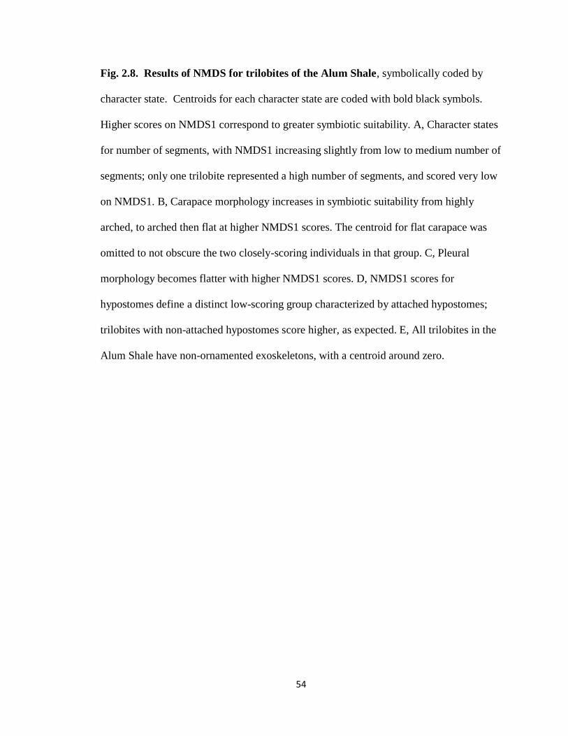
54
Fig. 2.8. Results of NMDS for trilobites of the Alum Shale, symbolically coded by
character state. Centroids for each character state are coded with bold black symbols.
Higher scores on NMDS1 correspond to greater symbiotic suitability. A, Character states
for number of segments, with NMDS1 increasing slightly from low to medium number of
segments; only one trilobite represented a high number of segments, and scored very low
on NMDS1. B, Carapace morphology increases in symbiotic suitability from highly
arched, to arched then flat at higher NMDS1 scores. The centroid for flat carapace was
omitted to not obscure the two closely-scoring individuals in that group. C, Pleural
morphology becomes flatter with higher NMDS1 scores. D, NMDS1 scores for
hypostomes define a distinct low-scoring group characterized by attached hypostomes;
trilobites with non-attached hypostomes score higher, as expected. E, All trilobites in the
Alum Shale have non-ornamented exoskeletons, with a centroid around zero.

55
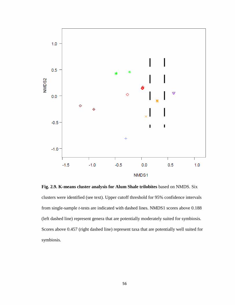
56
Fig. 2.9. K-means cluster analysis for Alum Shale trilobites based on NMDS. Six
clusters were identified (see text). Upper cutoff threshold for 95% confidence intervals
from single-sample t-tests are indicated with dashed lines. NMDS1 scores above 0.188
(left dashed line) represent genera that are potentially moderately suited for symbiosis.
Scores above 0.457 (right dashed line) represent taxa that are potentially well suited for
symbiosis.

57
Fig. 2.10. NMDS analysis for trilobites of the Alum Shale, comparing middle
Cambrian mostly oxic assemblages to late Cambrian–Early Ordovician mixed
assemblages. Middle Cambrian scores have a centroid slightly below zero on NMDS1,
while late Cambrian–Early Ordovician centroid is slightly above zero.
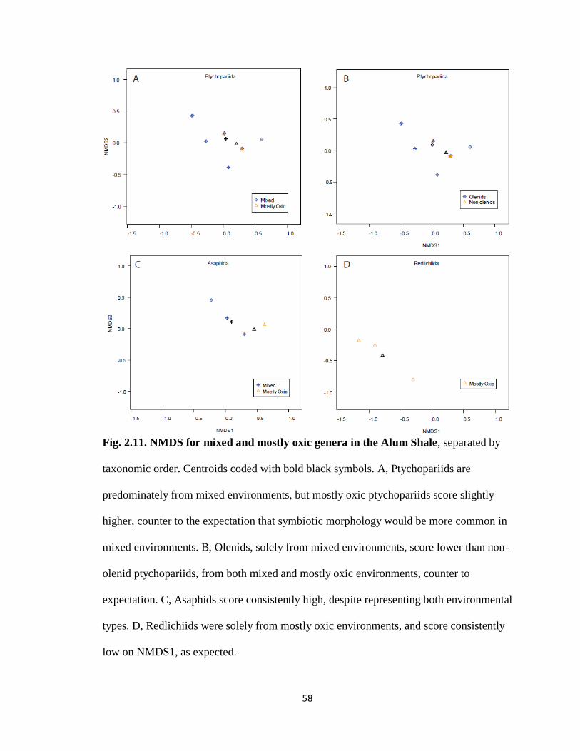
58
Fig. 2.11. NMDS for mixed and mostly oxic genera in the Alum Shale, separated by
taxonomic order. Centroids coded with bold black symbols. A, Ptychopariids are
predominately from mixed environments, but mostly oxic ptychopariids score slightly
higher, counter to the expectation that symbiotic morphology would be more common in
mixed environments. B, Olenids, solely from mixed environments, score lower than non-
olenid ptychopariids, from both mixed and mostly oxic environments, counter to
expectation. C, Asaphids score consistently high, despite representing both environmental
types. D, Redlichiids were solely from mostly oxic environments, and score consistently
low on NMDS1, as expected.
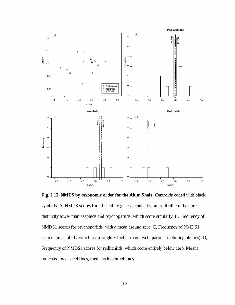
59
Fig. 2.12. NMDS by taxonomic order for the Alum Shale. Centroids coded with black
symbols. A, NMDS scores for all trilobite genera, coded by order. Redlichiids score
distinctly lower than asaphids and ptychopariids, which score similarly. B, Frequency of
NMDS1 scores for ptychopariids, with a mean around zero. C, Frequency of NMDS1
scores for asaphids, which score slightly higher than ptychopariids (including olenids). D,
Frequency of NMDS1 scores for redlichiids, which score entirely below zero. Means
indicated by dashed lines, medians by dotted lines.

60
Fig. 2.13. Effects of removing segmentation as a character for both trilobite NMDS
analyses. Original NMDS points plotted as triangles (with segments),with direction and
magnitude of shift indicated with lines after segmentation was removed from the
analysis. A, Shift in NMDS scores for the early-to-middle Cambrian trilobites. Shifts
were small, and scores did not shift uniformly negative, as expected if segments were
inflating original NMDS1 scores. B, Shift in NMDS scores for the middle Cambrian to
early Ordovician Alum Shale trilobites. Shifts were slightly larger than in A, but still
minor, and scores do not shift uniformly positive, as expected if segments were deflating
original NMDS1 scores.
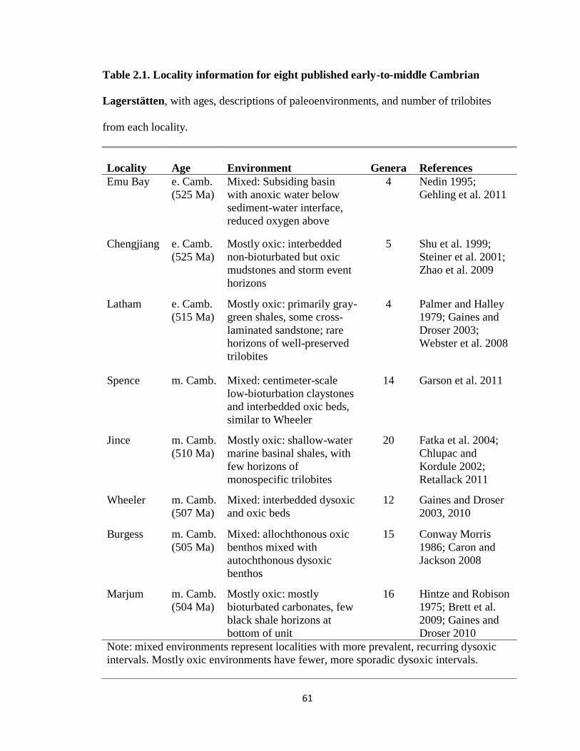
61
Table 2.1. Locality information for eight published early-to-middle Cambrian
Lagerstätten, with ages, descriptions of paleoenvironments, and number of trilobites
from each locality.
Locality Age Environment Genera References
Emu Bay e. Camb.
(525 Ma)
Mixed: Subsiding basin
with anoxic water below
sediment-water interface,
reduced oxygen above
4 Nedin 1995;
Gehling et al. 2011
Chengjiang e. Camb.
(525 Ma)
Mostly oxic: interbedded
non-bioturbated but oxic
mudstones and storm event
horizons
5 Shu et al. 1999;
Steiner et al. 2001;
Zhao et al. 2009
Latham e. Camb.
(515 Ma)
Mostly oxic: primarily gray-
green shales, some cross-
laminated sandstone; rare
horizons of well-preserved
trilobites
4 Palmer and Halley
1979; Gaines and
Droser 2003;
Webster et al. 2008
Spence m. Camb.
Mixed: centimeter-scale
low-bioturbation claystones
and interbedded oxic beds,
similar to Wheeler
14 Garson et al. 2011
Jince m. Camb.
(510 Ma)
Mostly oxic: shallow-water
marine basinal shales, with
few horizons of
monospecific trilobites
20 Fatka et al. 2004;
Chlupac and
Kordule 2002;
Retallack 2011
Wheeler m. Camb.
(507 Ma)
Mixed: interbedded dysoxic
and oxic beds
12 Gaines and Droser
2003, 2010
Burgess m. Camb.
(505 Ma)
Mixed: allochthonous oxic
benthos mixed with
autochthonous dysoxic
benthos
15 Conway Morris
1986; Caron and
Jackson 2008
Marjum m. Camb.
(504 Ma)
Mostly oxic: mostly
bioturbated carbonates, few
black shale horizons at
bottom of unit
16 Hintze and Robison
1975; Brett et al.
2009; Gaines and
Droser 2010
Note: mixed environments represent localities with more prevalent, recurring dysoxic
intervals. Mostly oxic environments have fewer, more sporadic dysoxic intervals.
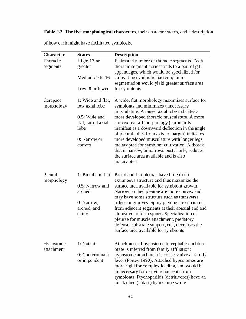
62
Table 2.2. The five morphological characters, their character states, and a description
of how each might have facilitated symbiosis.
Character States Description
Thoracic
segments
High: 17 or
greater
Medium: 9 to 16
Low: 8 or fewer
Estimated number of thoracic segments. Each
thoracic segment corresponds to a pair of gill
appendages, which would be specialized for
cultivating symbiotic bacteria; more
segmentation would yield greater surface area
for symbionts
Carapace
morphology
1: Wide and flat,
low axial lobe
0.5: Wide and
flat, raised axial
lobe
0: Narrow or
convex
A wide, flat morphology maximizes surface for
symbionts and minimizes unnecessary
musculature. A raised axial lobe indicates a
more developed thoracic musculature. A more
convex overall morphology (commonly
manifest as a downward deflection in the angle
of pleural lobes from axis to margin) indicates
more developed musculature with longer legs,
maladapted for symbiont cultivation. A thorax
that is narrow, or narrows posteriorly, reduces
the surface area available and is also
maladapted
Pleural
morphology
1: Broad and flat
0.5: Narrow and
arched
0: Narrow,
arched, and
spiny
Broad and flat pleurae have little to no
extraneous structure and thus maximize the
surface area available for symbiont growth.
Narrow, arched pleurae are more convex and
may have some structure such as transverse
ridges or grooves. Spiny pleurae are separated
from adjacent segments at their abaxial end and
elongated to form spines. Specialization of
pleurae for muscle attachment, predatory
defense, substrate support, etc., decreases the
surface area available for symbionts
Hypostome
attachment
1: Natant
0: Conterminant
or impendent
Attachment of hypostome to cephalic doublure.
State is inferred from family affiliation;
hypostome attachment is conservative at family
level (Fortey 1990). Attached hypostomes are
more rigid for complex feeding, and would be
unnecessary for deriving nutrients from
symbionts. Ptychopariids (detritivores) have an
unattached (natant) hypostome while

63
corynexochids and redlichiids (carnivores) have
attached (conterminant or impendent)
hypostomes
Exoskeletal ornamentation
1: No ornamentation
0: Spines or
pustules
Cuticle thickness was not directly observable for this study. Exoskeletal ornamentation, when
observed, was used as a substitute.
Ornamentation for predatory defense would be
unnecessary in sparsely-inhabited dysoxic
environments and would increase metabolic
costs during molting. Fortey argued a thin
cuticle decreased metabolic costs, thereby
making trilobites more symbiotically optimized

64
Table 2.3. Tests for independence of characters and relation of characters to
NMDS1 and to low oxygen conditions for both datasets. Pairwise correlations and
statistical significance for relationships of the five character-state values between each
other, between characters and NMDS1 scores, and strength of relationship between
character states and environmental conditions.
Character State Pairwise Correlations
(Spearman’s rho)
Character CM PM HA EO
Corr.
with
NMDS1
Relation to
oxic/mixed
conditions
(Kruskal-
Wallis chi-
squared)
Early-to-middle Cambrian
Segments
Statistic
p-value
0.03
0.82
0.05
0.67
0.41
<0.01
0.23
0.06
0.42
0.001
15.328
0.572
Carapace
morphology (CM)
Statistic
p-value
0.17
0.17
0.16
0.21
0.12
0.32
0.36
0.003
0.381
0.827
Pleural
morphology (PM)
Statistic
p-value
0.21
0.08
0.38
<0.01
0.57
<0.0001
1.480
0.477
Hypostome
attachment (HA)
Statistic
p-value
0.39
<0.01
0.84
<0.0001
2.490
0.115
Exoskeletal
ornamentation
(EO)
Statistic
p-value
0.61
<0.0001
0.332
0.565
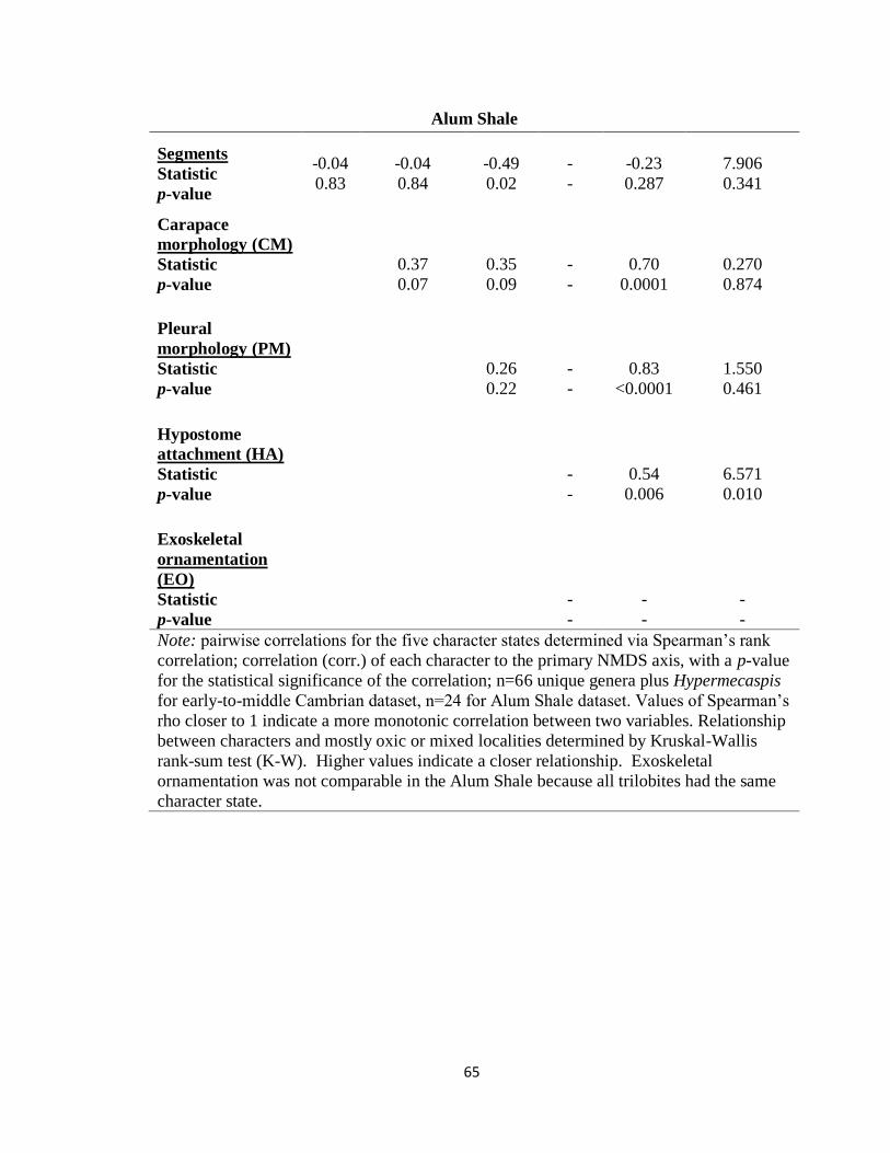
65
Alum Shale
Segments
Statistic
p-value
-0.04
0.83
-0.04
0.84
-0.49
0.02
-
-
-0.23
0.287
7.906
0.341
Carapace
morphology (CM)
Statistic
p-value
0.37
0.07
0.35
0.09
-
-
0.70
0.0001
0.270
0.874
Pleural
morphology (PM)
Statistic
p-value
0.26
0.22
-
-
0.83
<0.0001
1.550
0.461
Hypostome
attachment (HA)
Statistic
p-value
-
-
0.54
0.006
6.571
0.010
Exoskeletal
ornamentation
(EO)
Statistic
p-value
-
-
-
-
-
-
Note: pairwise correlations for the five character states determined via Spearman’s rank
correlation; correlation (corr.) of each character to the primary NMDS axis, with a p-value
for the statistical significance of the correlation; n=66 unique genera plus Hypermecaspis
for early-to-middle Cambrian dataset, n=24 for Alum Shale dataset. Values of Spearman’s
rho closer to 1 indicate a more monotonic correlation between two variables. Relationship
between characters and mostly oxic or mixed localities determined by Kruskal-Wallis
rank-sum test (K-W). Higher values indicate a closer relationship. Exoskeletal
ornamentation was not comparable in the Alum Shale because all trilobites had the same
character state.

66
Table 2.4. Number of thoracic segments by time and taxonomic order for
Cambrian through Early Ordovician trilobites (both datasets combined). Sample size,
minimum (Min), mean, maximum (Max) values, and standard deviations (SD) for
thoracic segmentation are given for each trilobite order. Total sample size, mean and
standard deviation for each time period is also given (Combined).
Time Period Taxonomic
Order
Sample
Size Min Mean Max SD
early Cambrian
Ptychopariids 3 10 12.67 15 2.52
Redlichiids 10 8 12.30 16 2.87
Combined 13 - 12.38 - 2.69
middle Cambrian
Corynexochids 15 2 7.33 11 2.02
Ptychopariids 36 8 13.83 31 4.12
Redlichiids 5 13 16.43 19 2.55
Asaphids 2 10 10.00 10 0.00
Combined 58 - 12.37 - 4.61
late Cambrian-
Early Ordovician
Ptychopariids 12 8 11.50 14 2.15
Asaphids 4 8 9.00 10 1.15
Combined 16 - 10.88 - 2.22
Note: Data represent 66 genera in the early-to-middle Cambrian data set and 24 genera
in the Alum Shale data set. Three genera were represented in both data sets, and these
duplicates were not included in this table.

67
CHAPTER 3
CAMBRIAN TRILOBITES AS ARCHIVES FOR ANTHROPOCENE BIOMARKERS
AND OTHER CHEMICAL COMPOUNDS1
___________________________
1 John, D. J., Medeiros, P. M., Babcock-Adams, L. C., and Walker, S. E. Submitted to
Anthropocene, April 18 2016.

68
Abstract
Molecular biomarkers reveal insights into biotic diversity in ancient ecosystems, yet most
biomarker analyses target only specific compounds. We used a multibiomarker approach
to examine a wide spectrum of organic molecules contained within exceptionally well-
preserved middle Cambrian trilobites and associated sediments from the Wheeler Shale.
We found an abundance of modern biomarkers, representing algal and plant sources, with
evidence of biomass burning. Additionally, anthropogenic compounds comprised up to
96% of all compounds present and included plasticizers, flame retardants, petroleum by-
products, and insect repellent. These compounds are usually discarded from analyses,
but we argue that they are essential for understanding the entire fossilization process.
The pervasiveness of terrestrial and anthropogenic chemicals suggests that these fossils
reveal more about Anthropocene-altered terrestrial landscapes than Cambrian oceans.
Introduction
Molecular biomarkers are a widely adopted biogeochemical tool to explore the
presence of ancient organisms that otherwise have no macro- or microscopic preservation
(Brocks and Summons, 2005; Brocks et al., 2005; Grice et al., 2005; Olcott et al;. 2005;
Pawlowska et al., 2012). Refractory biomolecules (and their derivatives) are used to
identify early Proterozoic microbial life, bacterial metabolic pathways and taxonomic
affinities (Brocks et al., 2005; Olcott et al., 2005; Brocks and Schaeffer, 2008; O’Malley
et al., 2013). Biomarkers characteristic of sulfur-oxidizing bacteria such as 16:1ω7c/t
and 18:1ω7c phospholipid fatty acids (Zhang et al., 2005) found in association with
trilobites could be used to support hypotheses of symbiosis with these organisms (Fortey,

69
2000). However, even if well preserved for millions of years, rocks and fossils collected
at or near the surface are exposed to modern compounds that could overprint the original
chemical fossil record (Wischmann et al., 2002; Rasmussen et al., 2008; French et al.,
2015). Those compounds are usually discarded from analyses, but we argue that they are
essential for understanding the fossilization process. Importantly, conventional
biomarker analyses target only specific compounds chosen a priori, but a multibiomarker
approach characterizes a wide range of molecular compound classes in an ecosystem
(Simoneit et al., 2014). This approach allows for a comprehensive characterization of the
biomarker record, with the potential to recognize unexpected signals that would be lost in
targeted biomarker analysis.
After a rigorous solvent cleansing regime to eliminate surficial contaminants, we
found extensive remaining chemical overprints from modern biomarkers and chemical
compounds in Cambrian trilobites and their associated sediments. These chemical
compounds reveal a dominantly terrestrial landscape altered by anthropogenic chemicals,
and little if anything about the Cambrian seas in which these trilobites lived. Effectively,
Anthropocene disturbance is not just at the landscape level, but also permeates through
groundwater, overprinting the original chemicals preserved in fossil exoskeletons. Such
overprints affect not only what we can discover about ancient ecosystems, but also reveal
perturbations concerning the modern environment under which calcareous fossils are
buried.

70
Methods
Trilobites were quarried commercially from the middle Cambrian Wheeler Shale by
professional collectors (West Desert Collectors and Terra Trilobites, Delta UT) from rock
depths up to 5 meters representing rock with little, if any, visible weathering. Two
specimens of Elrathia and 16 Peronopsis with robust and complete exoskeletons were
used (Fig. 3.1). The trilobites and their associated cone-in-cone encrustations were
separated from the underlying sediment, with both fossils and sediment being used for
analysis (Fig. 3.2). The 16 Peronopsis were combined into two sets of eight for analysis,
to yield a comparable sample mass to the Elrathia and ensure sufficient material for
analysis. Because compounds from anthropogenic polymers are particularly pervasive, to
minimize plastic contamination, two additional Elrathia kingii and five Peronopsis, both
with associated sediment, were collected and protected from contact with any type of
plastics during extraction, shipping, and handling. The five protected Peronopsis were
combined for analysis, but did not yield any compounds above the detection limit, despite
repeated tests on the sample material, and thus these samples could not be interpreted.
Total carbon for sediments was determined by powdering sediment samples
associated with both trilobite species in a Spex 8000 ball mill to produce approximately
20 ml of powdered sediment. 100 mg of these powders were weighed into a crucible
boat and fired on an Eltra furnace to 1350°C under a pure oxygen atmosphere. The
resultant carbon dioxide was measured by infrared absorption on an Eltra CS500
determinator to yield the total weight percent carbon in the sample. Total inorganic
carbon was then determined by weighing another 100 mg of the same sample powder into
a 250 ml flask and mixing with 10 ml of ethanol, then connecting the flask to an Eltra

71
CS500 determinator, adding 10 ml of 20% HCl and heating to 50°C, and measuring the
resultant carbon dioxide as above. Total organic carbon was determined by subtracting
the inorganic carbon from the total carbon for each sample, and averaging values by
species. Carbon and inorganic carbon analysis was performed at the Lyons Lab at UC
Riverside.
Sediment and exoskeletal samples were prepared for multibiomarker analysis by GC-
MS, yielding a profile of individual biomarkers present in each sample, following a
multibiomarker method established by Medeiros and Simoneit (2007; 2008a; 2008b) and
Simoneit et al. (2014). This method allows for a simultaneous characterization of the
different chemical classes spanning a wide range of polarities, without a need to isolate
certain chemical classes before analysis. Protected samples were rinsed with Milli-Q
water upon arrival, and after drying, they were gently rinsed with dichloromethane
followed by methanol and left to dry again at room temperature. All samples were
powdered in a solvent pre-cleaned ball mill and then weighed in a pre-combusted (450°C
for 5 h) beaker. Samples were then sonicated twice for 15 min in a 30 mL mixture of
dichloromethane:methanol (2:1, v/v). The extract aliquots were combined and filtered
using a Gelman Swinney filtration unit containing an annealed pre-combusted glass fiber
filter (42.5 mm, Whatman) for the removal of insoluble particles. The filtrate was first
concentrated in a RapidVap (solvent evaporation system) to about 1.5 mL, then further to
500 μL using a stream of high-purity nitrogen. Aliquots of the total extracts were
evaporated completely using a stream of filtered nitrogen gas, and then converted to their
trimethylsilyl derivatives using BSTFA containing 1% TMCS and pyridine for 3 h at

72
70°C. Immediately before GC-MS analysis, derivatized extracts were evaporated to
dryness using nitrogen gas and redissolved in hexane for injection.
Aliquots of 1 μL of silylated total extracts were analyzed within 24 hours using a HP
6890 gas chromatograph interfaced with a HP 5975 mass selective detector (GC-MS). A
DB5-MS capillary column (30 m x 0.25 mm I.D. and film thickness of 0.25 μm) was
used with helium as the carrier gas at a constant flow rate of 1.3 mL min-1. The injector
and MS source temperatures were maintained at 280°C and 230°C, respectively. The
column temperature program consisted of injection at 65°C and hold for 2 min,
temperature increase of 6°C min-1 to 300°C, followed by an isothermal hold at 300°C for
15 min. The MS was operated in the electron impact mode with an ionization energy of
70 eV. The scan range was set from 50 to 650 Da and the samples were analyzed in
splitless mode.
Data were acquired and processed with the HP-Chemstation software. Individual
compounds were identified by comparison of mass spectra with literature and library
data, comparison of mass spectra and GC retention times with those of authentic
standards and/or interpretation of mass spectrometric fragmentation patterns.
Compounds were quantified using the total ion current (TIC) peak area, and converted to
compound mass using calibration curves of external standards: n-eicosene for n-alkanes,
isoprenoids, UCM, and phthalates; n-hexadecanoic acid for n-alkanoic acids, n-alkanols
and glyceride derivatives; lupeol for diterpenoids, sterols and lignin derivatives; glucose
for monosaccharides; sucrose for disaccharides. A procedural blank was run in sequence
to samples, presenting no significant background interferences.

73
There was a higher percentage of natural biogenic compounds among protected
(65.84%) than unprotected (23.58%) exoskeletons and sediments, and anthropogenic
concentrations were likewise lower among protected specimens (Table 3.1; Appendix
3.1), indicating that collection protocols were successful in eliminating anthropogenic
contaminants introduced during or after collection. Therefore, remaining anthropogenic
compounds represent mainly those introduced to samples in situ.
Results and Discussion
Biogenic compounds in ancient trilobites
Our exoskeletal and sediment samples contained more than 50 molecular
biomarkers and anthropogenic organic compounds representing twelve chemical classes
(Appendix 3.1). Nine of the classes indicate biogenic input from either microorganism
biomass or terrestrial vegetation. Three classes were anthropogenic and in most samples
constituted the preponderance of the biomarkers by concentration (Fig. 3.3; Table 3.1).
Total carbon and organic carbon in the sediment were measured to quantify the
overall proportion of organic material from which biomarkers could be identified; total
carbon ranged from 3.69% by weight (Elrathia sediment) to 4.48% (Peronopsis
sediment), with total organic carbon comprising 0.35% and 0.33% by weight,
respectively. The similarity in organic carbon suggests that biomarker records between
species should be directly comparable.
Microorganism-derived biomarkers were abundant in sediments and particularly
in protected Elrathia exoskeletons, but nearly absent from unprotected exoskeletons
(Table 3.1). The presence of a low molecular-weight (≤ C20) homologous series,

74
especially n-alkanoic acids with a nearly total even-to-odd carbon preference (C14:0, C16:0,
C18:0), and to a lesser degree n-alkanes, n-alkanols, and glyceride derivatives are
indicative of microorganisms (Simoneit, 1977; Medeiros and Simoneit, 2008a). The
phytosterols stigmasterol and sitosterol were minor in our samples; whereas cholesterol
was found in slightly higher concentrations, especially in protected samples (Table 3.1).
Phytosterols are components of plant lipid membranes, but are also detected in
microalgae (Volkmann et al., 1998). Cholesterol is considered a major animal sterol
(Puglisi et al., 2003), but it is also a predominant compound in algal detritus (Goad, 1978;
Medeiros and Simoneit, 2008a), suggesting algae is the most likely source for all three
sterols.
Terrestrial plant biomarkers were present in protected and unprotected trilobites
(Figs. 3.4, 3.5; Table 1) and in sediments (Figs. 3.6, 3.7). The diterpenoid dehydroabietic
acid, a conifer-specific biomarker (Otto and Wilde, 2001), was detected in protected and
unprotected sediment and protected Elrathia exoskeletons (Table 3.1). Lignin derivatives
(vanillin and 3-methoxy-benzaldehyde; Opsahl and Benner, 1995) were also detected in
protected Peronopsis sediment, with vanillin occurring in unprotected sediments (Table
3.1). Because our methods do not include the oxidation/hydrolysis of biopolymers such
as lignin and cellulose, their detection in solvent-extractable samples indicates that
biomass burning may have released the monomer derivative products of biopolymers
(Medeiros and Simoneit, 2008b). Indeed, the anhydrosaccharide levoglucosan, a product
of burning cellulose from general plant biomass (Simoneit et al., 1999), was detected in
most of the samples, indicating that plant biomarkers may have been released by forest
wildfires overlying the buried fossils.

75
The carbon preference of n-alkanes suggests that the terrestrial plant record is
overprinted by another source. High molecular weight n-alkanes (> C20) with an odd-to-
even carbon preference indicate terrestrial biogenic input. However, an even-to-odd
carbon preference would point to plastic contamination (Simoneit et al., 2005). The lack
of a strong carbon number preference among the unprotected trilobites (Carbon
Preference Index, CPI = 0.7 – 0.8), combined with the abundant presence of plasticizers
(discussed below) suggests a mixture of both terrestrial and plastic inputs for the n-
alkanes (Table 3.1). The presence of C24, C26 and C28 n-alkanols (with an even-to-odd
carbon preference) indicate input from plant wax (Medeiros and Simoneit, 2008a).
Protected exoskeletons of Elrathia had saccharides, but not their unprotected
skeletons (Table 3.1). Especially, protected Elrathia sediment had the highest
saccharides present. This finding is unexpected, as sugars are readily consumed by
microbes and are generally not preserved in the rock record, suggesting the sugars are
modern (Swain et al., 1970; Chao et al., 2000). Saccharides were present in protected
Elrathia exoskeletons, though less abundantly than in sediments, and were absent in
unprotected exoskeletons (Fig. 3.4; Table 3.1). Glucose is the most common saccharide
present in the sediment and is the most abundant single component in protected Elrathia
sediment (Fig. 3.6; Table 3.1). Glucose is ubiquitous to all life and not diagnostic of any
source (Medeiros and Simoneit, 2007). Sucrose, indicative of general plant input, and
mycose, indicative of fungal input, occurred primarily in unprotected sediments (Table
1). It is likely that the saccharides were emplaced by groundwater before collection.
Anthropogenic compounds in ancient trilobites

76
Anthropogenic compounds represent the highest concentration of any compound
class overall, and was the predominant class in all exoskeletons (Fig. 3.3; Table 3.1).
Unprotected trilobites had more anthropogenic compounds (91.71% and 96.16% by
weight for Elrathia and Peronopsis, respectively) than protected Elrathia (44.72% by
weight). This difference indicates that protection protocols had some effect on limiting
anthropogenic contamination, but protected specimens still contained substantial amounts
of human-derived chemicals. The remaining anthropogenic compounds in protected
specimens represent in situ contamination before collection, indicating synthetic
chemicals are pervasive in the groundwater. Additionally, some contamination after
collection through airborne particles or incidental contact may have occurred despite
precautions.
Unprotected trilobites and protected Elrathia exoskeletons were generally
enriched in anthropogenic organophosphines and plasticizers relative to their associated
sediments (Table 3.1). Phthalates, which are plasticizers used in the plastic industry
(Wittasek et al., 2011), and triphenylphosphine oxide (TPPO), a flame retardant additive
in plastics (Weil and Levchik, 2009), were the most common anthropogenic markers
among all samples. Phthalates and organophosphines were, in general, also notably
higher in trilobite exoskeletons than sediments, with unprotected Peronopsis showing a
particular affinity for phthalates relative to unprotected Elrathia (55,638.2 10-9
g g-1
to
2400.0 10-9
g g-1
average concentration, respectively; Table 3.1).
Phthalates adsorb more readily onto microcrystalline calcite and clay particles
than on other siliciclastic sediments, mostly as a function of surface area (Sullivan et al.,
1982). Sediment, composed of clays and micrometer-scale calcite particles, would be

77
expected to have a much greater surface area, and therefore a higher concentration of
plasticizers, than in exoskeletons; however, that is not what we found. Because trilobites
had more organophosphines and plasticizers in their skeletons than in the surrounding
sediments, their microstructural properties could be particularly effective adsorbents for
organic compounds. Peronopsis also had higher concentrations of n-alkanes (probably
plastic-derived) relative to Elrathia. These results suggest that Peronopsis exoskeletons
have a greater affinity for organic adsorbates. Perhaps their exoskeletons are
microstructurally different from Elrathia, but we cannot discount that the difference is
related to our methods: we amalgamated five of the much smaller Peronopsis,
incorporating more surface area to yield equivalent sample mass to Elrathia.
Anthropogenic compounds were also found in the sediments, ranging from 73.73%
by weight in protected Peronopsis sediments to 3.81% by weight in protected Elrathia
sediments (Fig. 3.3; Table 1). Anthropogenic compounds in unprotected sediments
include m-toluamide and benzamide, which may be a degradation product of N,N-
Diethyl-meta-toluamide (DEET), an insect repellent (Pellegrino et al., 2011). An
unresolved complex mixture (UCM) was found in both unprotected and protected
sediments. UCMs are frequently associated with petroleum inputs (White et al., 2013;
Fig. 3.7; Supplementary Table 1), suggesting urban atmospheric particulates entrapped in
groundwater. Groundwater interaction may account for the introduction of plastics, as
phthalates are weakly water soluble when associated with dissolved organic
macromolecules such as humic acids and adsorb readily onto particulate surfaces in the
sediment, especially calcite and clays (Sullivan et al., 1982; Bauer et al., 1998; Huang et
al., 2008).

78
Conclusion
Our work highlights the potential for the biogeochemical record of fossils to be used
as a proxy for modern ecosystem change and Anthropocene alteration. Biomarkers and
other chemical compounds preserved in middle Cambrian trilobites revealed a modern
history of terrestrial forests and wildfires, petroleum by-products, fire-retardants, and
common insect repellants. These compounds can overprint the original biogenic signal
and are abundant throughout the environment. Preventative collection protocols and
extensive de-contamination of the samples yielded some reduction in anthropogenic
compounds, but not a substantial one. The use of multibiomarkers allowed us to capture
these additional data that are usually separated by fractionation and discarded from
biomarker analyses. We argue that the same preservational potential that makes fossils a
source of biomarker data also makes them susceptible to adsorption and accumulation of
anthropogenic chemicals. As these chemicals become more pervasive in the
environment, they have the potential to inhibit our ability to detect and reconstruct
ancient ecosystems, but provide a trove of information about perturbations in modern
ecosystems.
79
References
M. J. Bauer, R. Herrmann, A. Martin, H. Zellmann, Chemodynamics, transport behaviour
and treatment of phthalic acid esters in municipal landfill leachates. Water Sci.
Tech. 38 185-192 (1998).
J. J. Brocks, R. E. Summons, Biomarkers for early life. Biogeochemistry 8 63-115
(2005).
J. J. Brocks, G. D. Love, R. E. Summons, A. H. Knoll, G. A. Logan, S. A. Bowden,
Biomarker evidence for green and purple sulphur bacteria in a stratified
Palaeoproterozoic sea. Nature 437 866-870 (2005).
J. J. Brocks, P. Schaeffer, Okenane, a biomarker for purple sulfur bacteria
(Chromatiaceae), and other new carotenoid derivatives from the 1640 Ma Barney
Creek Formation. Geochim. Cosmochim. Acta 72 1396-1414 (2008).
L. Chao, P. Peng, G. Sheng, F. Jiamo, Precambrian organic matter. Chin. Sci. Bull. 45
295-303 (2000).
R. Fortey, Olenid trilobites: the oldest known chemoautotrophic symbionts? PNAS 97
6574-6578 (2000).
K. L. French, C. Hallmann, J. M. Hope, P. L. Schoon, J. A. Zumberge, Y. Hoshino, C. A.
Peters, S. C. George, G. D. Love, J. J. Brocks, R. Buick, Reappraisal of hydrocarbon
biomarkers in Archean rocks. Proc. Nat. Acad. Sci. 112 5915-5920 (2015).
L. J. Goad, The sterols of marine invertebrates: composition, biosynthesis, and
metabolites, in Marine Natural Products, P. J. Scheuer, Ed. (Academic Press,
London, 1978), pp. 75-172.

80
K. Grice, R. J. Twitchett, R. Alexander, C. B. Foster, C. Looy, A potential biomarker for
the Permian–Triassic ecological crisis. Earth Planet. Sci. Lett. 36 315-321 (2005).
P. C. Huang, C. J. Tien, Y. M. Sun, C. Y. Hsieh, C. C. Lee, Occurrence of phthalates in
sediment and biota: relationship to aquatic factors and the biota-sediment
accumulation factor. Chemosphere 73 539-544 (2008).
P. M. Medeiros, B. R. T. Simoneit, Analysis of sugars in environmental samples by gas
chromatography-mass spectrometry. J. Chromatogr. A 1141 271-278 (2007).
P. M. Medeiros, B. R. T. Simoneit, Multi-biomarker characterization of sedimentary
organic carbon in small rivers draining the northwestern United States. Org.
Geochem. 39, 52-74 (2008a).
P. M. Medeiros, B. R. T. Simoneit, Source profiles of organic compounds emitted upon
combustion of green vegetation from temperate climate forests. Environ. Sci.
Technol. 42 8310-8316 (2008b).
A. N. Olcott, A. L. Sessions, F. A. Corsetti, A. J. Kaufman, T. F. de Olivera, Biomarker
evidence for photosynthesis during Neoproterozoic glaciation. Science 310 471-473
(2005).
C. E. O’Malley, W. I. Ausich, Y. Chang, Isolation and characterization of the earliest
taxon-specific organic molecules (Mississippian, Crinoidea). Geology 41 347-350
(2013).
S. Opsahl, R. Benner, Early diagenesis of vascular plant tissues: lignin and cutin
decomposition and biogeochemical implications. Geochim. Cosmochim. Acta 59
4889−4904 (1995).
81
A. Otto, V. Wilde, Sesqui-, di-, and triterpenoids as chemosystematic markers in extant
conifers – a review. Bot. Rev. 67 141–238 (2001).
M. M. Pawlowska, N. J. Butterfield, J. J. Brocks, Lipid taphonomy in the Proterozoic and
the effect of microbial mats on biomarker preservation. Geology 41 103-106 (2012).
M. Pellegrino, N. Steinbach, M. C. Stensmyr, B. S. Hansson, L. B. Vosshall, A natural
polymorphism alters odour and DEET sensitivity in an insect odorant receptor,
Nature 478 511-514 (2011).
E. Puglisi, M. Nicelli, E. Capri, M. Trevisan, A. A. M. Del Re, Cholesterol, β-sitosterol,
ergosterol, and coprostanol in agricultural soils. J. Environ. Qual. 32, 466-471
(2003).
B. Rasmussen, I. R. Fletcher, J. J. Brocks, M. R. Kilburn, Reassessing the first
appearance of eukaryotes and cyanobacteria. Nature 45 1101-1104 (2008).
B. R. T. Simoneit, Diterpenoid compounds and other lipids in deep-sea sediments and
their geochemical significance. Geochim. Cosmochim. Acta 41 463-476 (1977).
B. R. T. Simoneit, J. J. Schauer, C. G. Nolte, D. R. Oros, V. O. Elias, M. P. Fraser, W. F.
Rogge, G. R. Cass, Levoglucosan, a tracer for cellulose in biomass burning and
atmospheric particles. Atmos. Environ. 33 173–182 (1999).
B. R. T. Simoneit, D. R. Oros, P. M. Medeiros, Organic matter provenance and
paleoenvironment in the Cretaceous on the Manihiki Plateau, South Pacific.
Palaeogeogr. Palaeoclimatol. Palaeoecol. 409 48-56 (2014).
B. R. T. Simoneit, P. M. Medeiros, B. M. Didyk, Combustion products of plastic as
indicators for refuse burning in the atmosphere. Environ. Sci. Technol. 39, 6961-
6970 (2005).

82
K. F. Sullivan, E. L. Atlas, C. S. Giam, Adsorption of phthalic acid esters from seawater.
Environ. Sci. Technol. 16 428-432 (1982).
F. M. Swain, J. M. Bratt, S. Kirkwood, Carbohydrates from Precambrian and Cambrian
rocks and fossils. Geol. Soc. Am. Bull. 81 499-504 (1970).
J. K. Volkman, S. M. Barrett, S. I. Blackburn, M. P. Mansour, E. I. Sikes, F. Gelin,
Microalgal biomarkers: a review of recent research developments. Org. Geochem.
29 1163–1179 (1998).
E. D. Weil, S. V. Levchik, Polystyrenes and Thermoplastic Styrene Copolymers. In
Flame Retardants for Plastics and Textiles (Carl Hanser Verlag, 2009), pp. 35-57.
H. K. White, L. Xu, P. Hartmann, J. G. Quinn, C. M. Reddy, Unresolved Complex
Mixture (UCM) in coastal environments is derived from fossil sources. Environ.
Sci. Technol. 47 726-731 (2013).
H. Wischmann, S. Hummel, M. A. Rothschild, B. Herrmann, Analysis of nicotine in
archeological skeletons from the Early Modern Age and from the Bronze Age. Anc.
Biomol. 4 47-52 (2002).
M. Wittassek, H. M. Koch, J. Angerer, T. Bruning, Assessing exposure to phthalates –
the human biomonitoring approach. Mol. Nutr. Fo od Res. 55 7-31 (2011).
C. L. Zhang, Z. Huang, J. Cantu, R. D. Pancost, R. L. Brigmon, T. W. Lyons, R. Sassen,
Lipid biomarkers and carbon isotope signatures of a microbial (Beggiatoa) mat
associated with gas hydrates in the Gulf of Mexico. Appl. Environ. Microbiol. 71
2106 (2005).
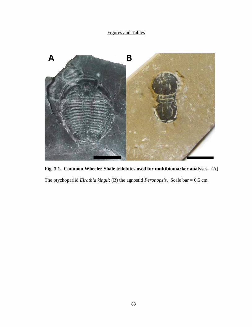
83
Figures and Tables
Fig. 3.1. Common Wheeler Shale trilobites used for multibiomarker analyses. (A)
The ptychopariid Elrathia kingii; (B) the agnostid Peronopsis. Scale bar = 0.5 cm.

84
Fig. 3.2. Location of samples. Exoskeleton (black) and cone-in-cone (blue; A) were
separated from sediments (B). Exoskeleton and cone-in-cone were pulverized and
analyzed together to yield data for Elrathia and Peronopsis, and sediment underneath
cone-in-cone was pulverized and analyzed separately for its data.

85
Fig. 3.3. Relative proportions of predominant biogenic and anthropogenic sources.
Calculated from mean concentrations by weight of compound classes for protected and
unprotected trilobite exoskeletons and associated sediment, and color coded by source
type.
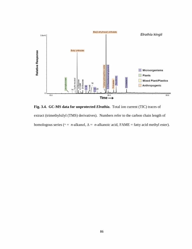
86
Fig. 3.4. GC-MS data for unprotected Elrathia. Total ion current (TIC) traces of
extract (trimethylsilyl (TMS) derivatives). Numbers refer to the carbon chain length of
homologous series (◦ = n-alkanol, Δ = n-alkanoic acid, FAME = fatty acid methyl ester).

87
Fig. 3.5. GC-MS data for unprotected Peronopsis. Total ion current (TIC) traces of
extract (trimethylsilyl (TMS) derivatives). Numbers refer to the carbon chain length of
homologous series (• = n-alkane, Δ = n-alkanoic acid, FAME = fatty acid methyl ester).

88
Fig. 3.6. GC-MS data for sediment associated with Elrathia. Total ion current (TIC)
traces of extract (trimethylsilyl (TMS) derivatives). Numbers refer to the carbon chain
length of homologous series (◦ = n-alkanol, Δ = n-alkanoic acid).

89
Fig. 3.7. GC-MS data for sediments associated with Peronopsis. Total ion current
(TIC) traces of extract (trimethylsilyl (TMS) derivatives). Numbers refer to the carbon
chain length of homologous series (◦ = n-alkanol, Δ = n-alkanoic acid, FAME = fatty
acid methyl ester, UCM = unresolved complex mixture).
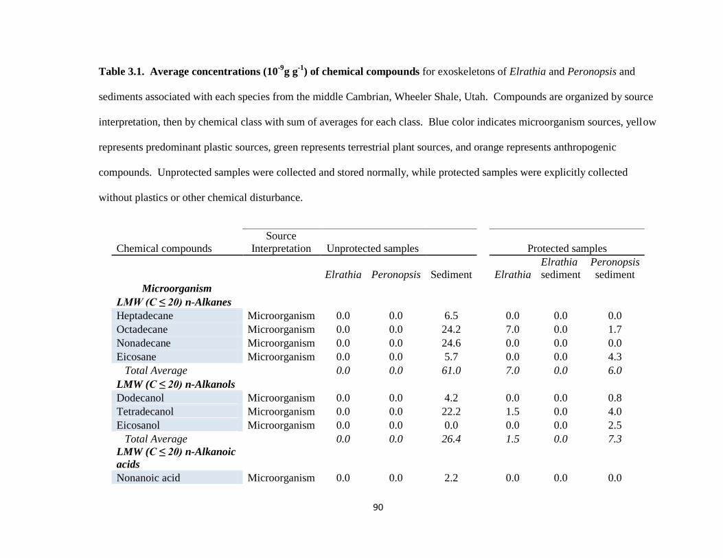
90
Table 3.1. Average concentrations (10-9
g g-1
) of chemical compounds for exoskeletons of Elrathia and Peronopsis and
sediments associated with each species from the middle Cambrian, Wheeler Shale, Utah. Compounds are organized by source
interpretation, then by chemical class with sum of averages for each class. Blue color indicates microorganism sources, yellow
represents predominant plastic sources, green represents terrestrial plant sources, and orange represents anthropogenic
compounds. Unprotected samples were collected and stored normally, while protected samples were explicitly collected
without plastics or other chemical disturbance.
Chemical compounds
Source
Interpretation Unprotected samples Protected samples
Elrathia Peronopsis Sediment Elrathia
Elrathia
sediment
Peronopsis
sediment
Microorganism
LMW (C ≤ 20) n-Alkanes
Heptadecane Microorganism 0.0 0.0 6.5 0.0 0.0 0.0
Octadecane Microorganism 0.0 0.0 24.2 7.0 0.0 1.7
Nonadecane Microorganism 0.0 0.0 24.6 0.0 0.0 0.0
Eicosane Microorganism 0.0 0.0 5.7 0.0 0.0 4.3
Total Average 0.0 0.0 61.0 7.0 0.0 6.0
LMW (C ≤ 20) n-Alkanols
Dodecanol Microorganism 0.0 0.0 4.2 0.0 0.0 0.8
Tetradecanol Microorganism 0.0 0.0 22.2 1.5 0.0 4.0
Eicosanol Microorganism 0.0 0.0 0.0 0.0 0.0 2.5
Total Average 0.0 0.0 26.4 1.5 0.0 7.3
LMW (C ≤ 20) n-Alkanoic
acids
Nonanoic acid Microorganism 0.0 0.0 2.2 0.0 0.0 0.0

91
Tridecanoic acid Microorganism 1.3 0.0 0.0 0.0 0.0 0.0
Tetradecanoic acid Microorganism 0.0 26.4 1.5 5.9 13.1 1.0
Hexadecanoic acid Microorganism 0.0 0.0 0.0 430.4 1243.2 10.6
Octadecanoic acid Microorganism 0.0 2.2 0.0 244.7 571.0 3.0
Total Average 1.3 28.6 3.7 681.0 1827.3 14.6
Sterols
Cholesterol Fauna/Algae 0.0 0.0 61.0 51.0 7.0 44.2
Stigmasterol Flora/Algae 0.0 0.0 0.0 0.0 0.0 5.2
Sitosterol Flora/Algae 0.0 0.0 5.1 0.0 0.0 0.0
Total Average 0.0 0.0 66.1 51.0 7.0 49.4
Glyceride derivatives
Glycerol Microorganism 0.0 0.0 4.3 0.0 0.0 0.0
1-O-Hexadecanoyl
glycerol Microorganism 0.0 0.0 17.7 15.9 0.0 6.5
1-O-Octadecanoyl glycerol Microorganism 0.0 0.0 2.5 0.0 0.0 1.1
Total Average 0.0 0.0 24.5 15.9 0.0 7.6
Total Average
Microorganism 1.3 28.6 181.7 756.4 1834.3 84.9
Plant
HMW (C > 20) n-Alkanes
Tetracosane Plastic mix 48.0 215.1 0.0 0.0 0.0 0.0
Pentacosane Plant 43.4 342.8 6.0 0.0 0.0 0.0
Hexacosane Plastic mix 63.6 482.4 0.0 0.0 0.0 0.0
Heptacosane Plant 45.8 410.4 0.0 0.0 0.0 0.0
Octacosane Plastic mix 30.6 335.5 0.0 0.0 0.0 0.0
Nonacosane Plant 25.1 226.6 0.0 0.0 0.0 0.0
Triacontane Plastic mix 15.1 162.2 0.0 0.0 0.0 0.0
Total Average 271.6 2175.0 6.0 0.0 0.0 0.0
HMW (C > 20) n-Alkanols
Docosanol Plant 0.0 0.0 0.0 0.0 0.0 2.8

92
Tetracosanol Plant 0.0 0.0 0.0 0.0 0.0 5.4
Hexacosanol Plant 2.9 0.0 57.1 9.6 0.0 18.4
Octacosanol Plant 7.1 0.0 26.7 9.9 0.9 23.0
Total Average 10.0 0.0 83.8 19.5 0.9 49.6
Saccharides
Glucose
General
biomass 0.0 0.0 233.0 274.2 3914.1 2.7
Fructose Plant 0.0 0.0 0.0 0.0 560.3 0.0
Levoglucosan Plant burning 0.0 48.6 2.4 1.8 15.7 1.2
Sucrose Plant 0.0 0.0 189.8 14.0 22.5 2.1
Total Average 0.0 48.6 425.2 290.0 4512.6 6.0
Lignin derivatives
3-Methoxy-benzaldehyde Plant 0.0 0.0 0.0 0.0 0.0 8.2
Vanillin Plant 0.0 0.0 1.4 0.0 0.0 3.9
Total Average 0.0 0.0 1.4 0.0 0.0 12.1
Diterpenoids
Dehydroabietic acid Conifer 0.0 0.0 3.0 2.8 1.0 2.5
Total Average Plant 281.6 2223.6 519.4 312.3 4514.5 70.2
Anthropogenic
Amides
Benzamide Insect repellent 0.0 0.0 5.2 0.0 0.0 0.0
m-Toluamide Insect repellent 0.0 0.0 4.2 0.0 0.0 0.0
Total Average 0.0 0.0 9.4 0.0 0.0 0.0
Organophosphines
Tributylphosphine Anthropogenic 9.2 23.8 0.0 0.0 0.0 0.0
Triphenylphosphine oxide
Flame
retardant 722.3 710.9 10.1 35.0 14.1 15.4
Total Average 731.5 734.7 10.1 35.0 14.1 15.4
Plasticizers
Terephthalic Acid Plastics 0.0 58.7 23.1 0.0 0.0 0.0

93
Butyl phthalate Plastics 1649.1 41349.9 185.7 197.1 45.1 204.7
Butyl hexyl phthalate Plastics 36.4 934.3 138.8 48.6 36.1 52.6
Bis(2-ethylhexyl) phthalate Plastics 714.4 13137.8 127.9 583.8 156.0 162.6
Phthalic Anhydride Plastics 0.0 157.5 0.0 0.0 0.0 0.0
Total Average 2399.9 55638.2 475.5 829.5 237.2 419.9
Total Average
Anthropogenic
3131.4 56372.9 495.0 864.5 251.3 435.3
% biogenic 8.29 3.84 58.62 55.28 96.19 26.27
All unprotected: 23.58 All protected: 65.84
% anthropogenic 91.71 96.16 41.38 44.72 3.81 73.73
All unprotected: 71.42 All protected: 34.16
CPIa for n-alkanes 0.7 0.8 - - - -
aCarbon Preference Index: CPI = (C23+C25+C27+C29)/(C24+C26+C28+C30).
Average values represent the mean of individual concentrations given in Table S1 for each type of protected and
unprotected sample.
94
CHAPTER 4
DIAGENESIS AND ELEMENTAL CHEMISTRY OF EXCEPTIONALLY
PRESERVED PUTATIVELY DYSOXIC TRILOBITES FROM THE WHEELER
SHALE1
___________________________
1 John, D. J. and Walker, S. E. To be submitted to Palaios.
95
Abstract
Trilobites from the middle Cambrian Wheeler Shale, Utah, are exceptionally well
preserved. A previous sedimentary model suggested that bacterial sulfate reduction
acting on decaying trilobites led to cone-in-cone calcite (CIC) precipitation that
buttressed the ventral side of the exoskeletons in early diagenesis. In addition to the
sediments, it is quite possible that the exoskeletons themselves might hold geochemical
and petrographic signatures consistent with this model. We examined two trilobite
species, benthic Elrathia kingii and putatively pelagic Peronopsis interstricta to
determine if they had different petrographic and geochemical signatures potentially
reflecting their habitats prior to burial or if they had similar signatures indicative of early
burial diagenesis. Similarly, we examined whether non-molted trilobites with
presumably more organic carbon had different petrographic and geochemical signatures
than molts and exoskeletal fragments. We found no textural differences in CIC between
species or between molts and non-molted trilobites, but CIC was thinner on exoskeletal
fragments, suggesting that organic carbon was diffuse throughout the sediment and
exoskeletons acted as nucleation points for CIC. Low-pressure zones between sediment
layers also seemed to play a role in governing CIC formation. Cone-in-cone calcite
displaced compacted and cohesive sediment, indicating compaction preceded CIC
precipitation. Cubic pyrite inclusions within CIC suggest low-organic carbon conditions,
which favor cubic pyrite over framboidal, also must have preceded CIC formation.
Elemental Ca, Mg, Fe and S compositions of both trilobite species’ exoskeletons were
similar, despite differences in their ecological habits, suggesting that original calcite
compositions have been overprinted by diagenetic recrystallization. Low sulfur content
96
in all specimens suggests calcites precipitated under euxinic conditions. Calcite twins in
the CIC indicate a thermal history between 170 and 200 °C. Our findings support
previous interpretations of CIC formation under sulfate-reducing conditions, but suggest
that CIC was governed by late diagenetic or low-grade metamorphic processes, in
response to localized decreases in overburden pressure, increased temperatures,
porewater diffusion transporting alkalinity, and favorable thermodynamics for the
nucleation of calcite along exoskeletons.
Introduction
Fossils from the Wheeler Shale of southwestern Utah reveal an unusual
taphonomic window into the middle Cambrian of Laurentia (Robison, 1971). In
particular, the trilobites are thought to be relatively pristine, are very abundant in certain
horizons and usually have characteristic cone-in-cone calcite (CIC) that underplates their
exoskeletons (Walcott, 1908; Bright, 1959; Gaines and Droser, 2003; Brett et al., 2009).
This unusual preservation is attributed to the physical and geochemical conditions of the
Cambrian paleoenvironment. Depositional and preservational conditions of the Wheeler
Shale bear similarities to the Burgess Shale (Briggs et al., 2008), which has been
interpreted as greenschist-grade metamorphism based on evidence such as the presence
of muscovite, lack of clays and reduced organic carbon (Powell, 2003). Gaines and
Droser (2003) attribute the clay mineralogy in the Wheeler Shale to processes of burial
diagenesis. However, the metamorphic history of the Wheeler Shale has not been
examined, and changes in pressure and temperature conditions could play a role in the
unique preservation of these trilobites.

97
Oxygen may also play a role in preservation. The Wheeler Shale environment has
long been considered dysoxic (Bright, 1959; Brett et al., 2009). Cambrian atmospheric
oxygen levels were slightly below modern averages (~<20% O2; Berner et al 2003),
while CO2 levels were an order of magnitude higher (~4200 ppm, Bao et al., 2008; ~5000
ppm, Pörtner et al., 2004; cf. modern values ~400 ppm). Increased atmospheric CO2
would have several effects on Cambrian ocean dynamics, such as increased temperatures
that cause reduced seawater circulation and stratification of bottom waters, an increase in
terrestrial weathering, particularly carbonate flux to the oceans, and a reduction in oxygen
solubility in the ocean. However, fluctuations between anoxic, dysoxic, and fully oxic
conditions likely occurred in the Wheeler Shale, affecting both the composition of the
benthic community and their preservational pathways (Gaines and Droser, 2003; Gaines
et al., 2005; Gaines and Droser, 2010). Throughout its ~100-150m thickness (Robison,
1964), the Wheeler Shale is divided into discrete anoxic, dysoxic, and oxic taphofacies,
with different styles of preservation and different characteristic assemblages in each
(Gaines et al. 2005). Burgess Shale-type soft body preservation was described in the
anoxic facies. The dysoxic facies occurs primarily as thin beds, transitional from oxic to
anoxic, abundant with the trilobites Elrathia kingii and Peronopsis interstrictus. In the
dysoxic facies, where we focus in this study, Gaines et al. (2005) suggested that bacterial
sulfate reduction of organic carbon in the sediment was constrained within trilobite
exoskeletons, thereby facilitating the growth of CIC, enhancing trilobite preservation.
Sedimentological and ichnofabric analyses corroborated their preservation model, but the
fossils and CIC themselves have not been examined for direct evidence of either bottom-
water dysoxia or porewater euxinia.

98
Petrographic analyses of trilobite exoskeletons can be used to test predictions about
their preservational histories. First, Wheeler Shale trilobites are known to have
recrystallized calcite (Gaines et al., 2005), consistent with early diagenesis in a
carbonate-saturated environment. However, if their exoskeletons or CIC exhibit other
diagenetic textures more suggestive of later processes, it might suggest a more complex
diagenetic history that changes the interpretation of CIC formation. Associated pyrite
can be used as an indicator of diagenetic timing and conditions, with framboidal pyrite
representing sulfate-reducing conditions early in diagenesis, while cubic pyrite is more
representative of late diagenesis in sediments with low organic carbon contents (Taylor
and Macquaker, 2000). Second, if CIC is controlled primarily by the amount of bacterial
sulfate-reduction, then it should be thicker on complete specimens (with abundant soft
tissues) and thinner on molts or exoskeletal fragments that were buried with presumably
less organic carbon. Lastly, CIC typically grows on the ventral surfaces of trilobite
exoskeletons (Gaines et al., 2005), putatively in response to limited diffusion of
porewaters. Therefore, if CIC grows on the dorsal surface where porewaters are not
constrained, some other mechanism for CIC must be invoked.
The geochemistry of the exoskeletons and associated CIC can also reveal similarities
and differences in preservation among trilobite species. We examined Elrathia kingii, a
benthic trilobite, and Peronopsis interstricta, a putatively pelagic trilobite (Robison,
1971; the species has also been assigned to the genus Itagnostus; Naimark, 2012), to
determine if their exoskeletons yielded different elemental geochemistries consistent with
their life modes. Conversely, similar geochemistries among species and CIC would be
consistent with diagenetic overprint of the original exoskeletal calcite in anoxic

99
sediments. We examined several elements (Fe, Mg, S, Ca, C and Si) to attempt to
constrain their preservational modes. Iron and Mg were measured to constrain
oxygenation: Mg is abundant and well-mixed through the oceans (Tipper et al., 2006),
whereas Fe is more abundant in dysoxic benthic waters where it can accumulate by flux
from dysoxic sediments (Salomons et al., 1987). A higher amount of Fe relative to Mg in
exoskeletons would suggest that calcites precipitated in more dysoxic waters. Sulfur was
also measured to indicate euxinia. Sulfate is common in oxic waters (Millero, 1974) and
becomes incorporated into calcites (Burdett et al. 1989; Marenco et al., 2008), while in
euxinic waters sulfate is reduced to sulfide which does not incorporate.
Calcites precipitated under euxinic conditions should show a lack of sulfur relative
to oxic calcites (Marenco et al., 2008). Calcium concentrations indicate overall cation
substitution, with lower Ca values representing greater cation substitution, a function
controlled linearly by temperature and pressure (Stehli and Hower, 1961). Calcites with
similar Ca values thus have similar overall substitution rates and their concentrations for
other elements can be compared directly to one another. Silicon in calcites represents
silicification, indicating diagenetic alteration. Carbon distributions were used to
determine if there were regions of the trilobite with more abundant C (possibly
representing soft-tissue structures such as the gut) that could influence CIC growth. Our
work yields additional understanding of the pathways of preservation in the Wheeler
Shale, confirming and expanding upon previous studies.

100
Methods
Elrathia kingii and Peronopsis interstricta and their surrounding sediments were
obtained from commercial collectors (following Gaines and Droser, 2003). Samples
were collected from fresh exposures in private quarries and represent multiple
fossiliferous dysoxic horizons, though no specific stratigraphic context was recorded for
specimens. Three whole and three molts (missing librigenae) of E. kingii and two whole
P. interstricta (hereafter referred to as Elrathia and Peronopsis, respectively) were used
for petrographic and geochemical analysis. Uncoated and polished petrographic thin
sections representing longitudinal and transverse glabellar sections of Peronopsis and
longitudinal and transverse glabellar and thoracic sections for Elrathia were used in
petrographic thin section and geochemical analysis (Fig. 4.1). These sections allow for
determination of average geochemical values that account for any heterogeneity in the
exoskeletons. Petrographic analysis included observations examining the relationships
between exoskeletons, CIC, and the surrounding sediment. Sediments in thin sections
also contained fragments of trilobite exoskeletons that were examined where exposed.
Thin sections were examined using a Leica DME petrographic microscope at 40-100x
magnification. The number of specimens was determined by the best-preserved
specimens; because of the lack of stratigraphic resolution, our samples may not be
adequately representative of the overall dysoxic taphofacies.
To determine if Elrathia and Peronopsis exoskeletons preserved signatures of
their original seawater chemistries, and thus had different geochemical signatures than
associated diagenetic CIC, their elemental chemistry was examined. After petrographic
analysis, the thin sections were carbon-coated and analyzed on a JEOL JXA 8600

101
Superprobe electron microprobe with wavelength-dispersive X-ray spectroscopy (WDS),
which yields data to a precision of 0.01 weight percent. Elemental weight percent was
determined for Fe, Mg, Ca, and S within the cephalic, thoracic, and pygidial regions of
the trilobite exoskeletons, CIC, and associated sediments to constrain seawater
oxygenation and possible euxinia. Data were averaged within those three sample types
and by species and molt status. Forty-four point sample zones approximately 5-10 μm
wide were analyzed for 60 to 90 seconds with one to three analyses performed on each
point. Additional analysis time did not substantially increase detection limits. Precisions
as measured using a C.M. Taylor Calcite standard were ±0.04 for Ca, ±<0.01 for Mg,
±0.06 for Fe, and ±0.01 for S. Average approximate detection limits were 0.03 weight
percent for Ca, 0.03 for Mg, 0.11 for Fe, and 0.01 for S. All data were above detection
limits except for S.
Elemental maps provide additional data about distributions of elements in trilobite
exoskeletons than point analyses alone provide. Elemental maps were made for S, Si,
and Ca on the electron microprobe using energy-dispersive X-ray spectroscopy (EDS),
across sections that had sediment, exoskeleton, and CIC in close association, to
differentiate between sulfides, siliciclastics, and calcium carbonates, respectively.
Relative depletion or enrichment of S between sample groups might suggest those
samples formed under differing conditions of euxinia. Silicon in the CIC and
exoskeleton would indicate either inclusions of siliceous sediment suggesting
deformation of the exoskeleton or silicification of the original calcite indicating
diagenetic alteration.
102
One specimen each of non-molted Peronopsis and Elrathia were used in carbon
elemental mapping using an environmental scanning electron microscope (ESEM),
because carbon cannot be examined on the electron microprobe, where specimens are
carbon-coated. Carbon concentrations could represent the vestiges of soft tissues
associated with microbially-mediated CIC precipitation, or variations in the organic
carbon content of the sediment. Trilobites were cleaned of surficial sediment and dried at
70 °C overnight before ESEM analysis. Dorsal exoskeletons were mapped using energy-
dispersive X-ray spectroscopy (EDS) on a Zeiss 1450SP ESEM. Elemental maps and
SEM backscatter images were obtained for the cephalon, thorax, and pygidium for both
species.
Total organic carbon for the sediments was determined by subtracting total inorganic
carbon from total carbon. Total carbon was determined by powdering a total of 25
sediment samples associated with both trilobite species in a Spex 8000 ball mill to
produce approximately 20 ml of powdered sediment. 100 mg of these powders were
weighed into a crucible boat and fired on an Eltra furnace to 1350°C under a pure oxygen
atmosphere. The resultant carbon dioxide was measured by infrared absorption on an
Eltra CS500 determinator to yield the total weight percent carbon in the sample. Total
inorganic carbon was then determined by weighing another 100 mg of the same sample
powder into a 250 ml flask and mixing with 10 ml of ethanol, then connecting the flask to
an Eltra CS500 determinator, adding 10 ml of 20% HCl and heating to 50°C, and
measuring the resultant carbon dioxide as above. Total organic carbon values were
averaged by species. Carbon and inorganic carbon analysis was performed at the Lyons
Lab at UC Riverside, and are the same as described in Chapters 2 and 5.

103
Results
Petrographic Analysis of Exoskeletons, Cone-in-cone Calcite and Sediment
Both Elrathia and Peronopsis exoskeletons had the same basic composition: a
thin (~10-25 m), mostly calcitic exoskeleton (with minor silica replacement, see next
section) (Fig. 4.2A). Cone-in-cone calcite projected usually from the ventral surface, but
grew also from the upper surface of exoskeletons (Fig. 4.2B-C). Crystals of CIC were
often optically continuous on both sides of exoskeletons, indicating the crystals were
genetically related and grew outward from the same nucleation site, i.e. the exoskeleton
(Fig. 4.2B-C).
Cone-in-cone calcite is also associated with trilobite exoskeletal fragments (Fig.
4.3). These fragments had CIC growth considerably thinner (mean thickness 0.34 mm)
than articulated trilobites (mean thickness 2.46 mm). Additionally, CIC growth occurred
on either side of the trilobite fragment (Fig. 4.3A–B).
Exoskeletons generally exhibited little deformation, but one Elrathia specimen’s
pleural segments were deflected downward under the adjacent pleurae and into the CIC,
suggesting lateral compression (Fig. 4.4A). Separate CIC crystals fill the space above
and below the deflected pleurae, and a third also partially separates the exoskeleton from
sediments deflected down alongside it.
Microstylolites are also found in some specimens (Fig. 4.4A) These structures
form when increased pressure drives dissolution and remobilization of carbonate and
concentrates insoluble phases such as clays along irregular wavy margins (Wanless,
1979). Crystals of CIC contained calcite twins (Fig. 4.4B). These twins are typically
widely-spaced thin twins, though some cones may have more developed twinning with

104
densely-packed thick twins. Sparse thin twinning is indicative of lower-temperature
deformation of the calcite, with a maximum thermal history of ~170 °C, while thick
tabular twins indicate slightly higher temperatures up to 200 °C (Ferrill et al., 2004;
Rybacki et al., 2013). Series of bedding-parallel fractures can be found in the CIC (Fig.
4.4).
Cone-in-cone calcite also contained sulfides as cubic crystals that did not interrupt
the CIC structure (Figs. 4.5A-B). Elemental analysis of these inclusions using WDS
showed a stoichiometry of FeS2, suggesting they are pyrite or marcasite.
The sediment surrounding both Peronopsis and Elrathia was a mix of siliciclastic
clays and fine-grained carbonates that is foliated roughly parallel to bedding (Fig. 4.6).
Sediment was cohesive and responded to stress by deforming plastically, not through
brittle fracturing or shearing through layers. Cone-in-cone calcite underneath trilobite
exoskeletons deflected nearby sediment and grew laterally outward between the deflected
sediment layers (Fig. 4.7). Foliations in the sediment are bedding-parallel except under
CIC growth, where foliations were sheared and rotated downward under the CIC crystal
(Fig. 4.7A). Foliated layers remained discrete and continuous through the zone of
shearing, indicating sediments were coherent but not fully lithified prior to CIC growth.
Individual sigmoidal or banded crystals of CIC grew in the shear zone between the
rotated sediment horizons (Figs. 4.7A-B). Microstylolites were observed, as previously
described for Fig. 4.4A, that indicated pressure dissolution of CIC calcite under vertical
strain.

105
Elemental Geochemistry of Exoskeletons, Cone-in-cone Calcite, and Sediment
The geochemistry of the exoskeletons, CIC, and sediment indicated the
similarities and differences in preservational histories. Broadly, the elemental
compositions of the exoskeleton and CIC were similar (Table 4.1).
Mean Ca exoskeletal and CIC values for non-molted Peronopsis, non-molted
Elrathia, and molted Elrathia were similar. Wilcoxon rank-sum tests revealed that Ca
values were not significantly different between exoskeletal groups (p = 0.965, df = 18,
W=41 between Peronopsis and molted Elrathia; p = 0.108, df = 19, W=64 between
Peronopsis and non-molted Elrathia; p = 0.223, df = 21, W=73 between non-molted and
molted Elrathia; α = 0.05). Exoskeleton Ca for all three groups was likewise not
significantly different from associated CIC values (p = 0.267, df = 10, W=13 for
Peronopsis; p = 0.343, df = 15, W = 30 for non-molted Elrathia; p = 0.121, df = 12, W =
18 for molted Elrathia; α = 0.05).
Iron and magnesium were slightly more concentrated in exoskeletons (mean 0.47
wt. % and 0.49 wt. %, respectively) than in CIC (mean 0.27 wt. % and 0.16 wt. %,
respectively; Table 4.1; Fig. 4.8). Those differences were not found significant by
Wilcoxon rank-sum test for Fe (p = 0.118, df = 37, W = 159) but were significantly
different for Mg (p << 0.001, df = 37, W=221). Sulfur was at or below detection limits
(0.01 wt. %) for 32 of the 44 samples, and of the remaining twelve, only six were more
than 0.02 wt. % (Fig. 4.8; Appendix 4.1).
Within the exoskeletons, molted Elrathia had the most Mg (mean 0.63 wt. %)
compared to non-molted Elrathia (mean 0.49 wt. %); non-molted Peronopsis had the
least (mean 0.31 wt. %; Table 4.1). However, Fe had higher values in Peronopsis (mean
106
0.59 wt. %) compared to non-molted Elrathia (mean 0.45 wt. %), while molted Elrathia
had the least Fe (mean 0.38 wt. %; Table 4.1; Fig. 4.8). A Wilcoxon rank-sum test
indicated molted Elrathia and Peronopsis exoskeletons were significantly different for
Mg (p < 0.001, df = 18, W = 77), while non-molted Elrathia and Peronopsis
exoskeletons were significantly different for Fe (p = 0.016, df = 19, W = 73).
Sediment composition was a mix of carbonates and siliciclastics, in contrast to the
relatively pure calcite of the CIC and exoskeletons, and thus showed markedly different
overall average values for Ca, Fe, and Mg (Fig. 4.8; Table 4.1). However, the
heterogeneity of the sediment also suggests that the small sample size may not describe
the overall variation of sediment well enough for confident statistical analysis.
Electron microprobe EDS elemental maps of both non-molted Elrathia (Fig.
4.9A-B) and Peronopsis (Fig. 4.9C-D) exoskeletons indicated partial silicification of the
exoskeleton in isolated locations; silicification is uncommon (< 5% of overall
exoskeleton calcite of all types within the 8 thin sections examined) and generally
restricted to patches of a few hundred μm. Under ESEM mapping, carbon had no
zonation that could be attributed to distributions of soft tissue either within or around the
exoskeleton, but only followed the difference between the more calcareous exoskeleton
and less calcareous sediment (Fig. 4.10)
Total organic carbon (as measured in Ch. 5) was 0.35% and 0.33% by weight,
respectively, for sediment associated with Elrathia and Peronopsis.

107
Discussion
The exceptional preservation in the Wheeler Shale has been described as a
function of its sedimentology, oxygenation, and the chemical changes associated with
bacterial sulfate reduction (Gaines and Droser, 2003). Wheeler Shale is described as a
fluctuating environment with repeating progressions among anoxic facies with finely
laminated sediment with soft-body preservation, dysoxic facies with monotypic, high-
density assemblages of Elrathia with Peronopsis in weakly bioturbated sediment, and
fully oxic facies with more diverse but sparse assemblages of trilobites in bioturbated
sediments (Gaines and Droser, 2003). After burial, reservoirs of porewater conducive to
CIC precipitation formed under trilobite exoskeletons, where sulfate reduction of organic
carbon in dysoxic sediments drove changes in the local geochemistry, enhancing the
occlusion of surrounding pore space and isolation of the trilobites and leading to CIC
formation and exceptional preservation.
We evaluated these sedimentological and paleoecological interpretations with
petrographic and geochemical data. We explored how the sedimentary, CIC, and
exoskeletal records describe the controls on CIC precipitation and the
paleoenvironmental and diagenetic conditions under which the trilobites were preserved.
Controls on Cone-in-Cone Precipitation
Our findings suggest that physical constraint of porewater alone cannot explain all
the textures seen in the CIC. Rather, sediment may not have been completely occlusive
to porewater flow, and geochemical gradients would not be totally contained by trilobite
exoskeletons. This is consistent with experimental results that show tightly packed clays

108
can still allow ionic diffusion at rates of cm per month (Oscarson, 1994). Tightly-packed,
deflocculated clays are part of the Gaines et al. (2005) pore-occlusion model for CIC
formation, though diffusion at the rates found by Oscarson (1994) would be sufficient to
carry alkalinity away from exoskeletons as it formed. Sediment also demonstrated
evidence of plastic deformation where CIC growth deflected it, which suggests
intergranular space was not completely sealed with authigenic cements.
While trilobite exoskeletons and sclerites may have provided some partial barrier
to upward diffusion, their exoskeletons may have also provided a nucleation template that
would have facilitated CIC growth. Such a mechanism has been described
experimentally, where calcite crystals provide an effective seed site for nucleation of
calcite from solution, and the growth rate from supersaturated fluids is dependent on the
degree of supersaturation (Lioliou et al., 2007). In sediments where BSR was ubiquitous,
fluids could be somewhat concentrated by retardation of upward diffusion under trilobite
exoskeletons, and become more supersaturated. Additionally, the cohesive, laminated
sediment and bedding-parallel fractures and microstylolites in the CIC suggest it was
formed after compaction, with a component of vertical stress. Microstylolites in
particular indicate a vertically oriented stress sufficient to cause calcite to undergo
pressure dissolution and loss of CIC material.
Twinning in the CIC indicates thermal stress: thermal alteration as high as 200 °C
produced thick twins, though most twins were thin twins that only suggest a thermal
maximum of 170°C. The thermal history of the CIC is likely close to the 200 °C
threshold, enough to begin partially developing thick twins but not completely lose thin-
twinned textures. Additionally, the concentration of twins in the lower part of CIC
109
structures (which is the oldest CIC, as it expands downward from the precipitation
surface along the trilobite carapace; Seilacher, 2001) suggests that CIC may have
precipitated under high-temperature conditions. Older CIC near the bottom of
encrustations would have more time to develop well-defined twins. Concave-downward
exoskeletons could have partially distributed these stresses outward, creating a lower-
pressure zone under the carapace more conducive to CIC formation. Combined with a
favorable site for nucleation, these factors could generate thicker growth of CIC than on
dorsal surfaces (Fig 4.11).
Conversely, thickness of encrustations was similar between molted and non-
molted specimens, while those of disarticulated sclerites were markedly thinner. Non-
molted trilobites would presumably be buried with abundant soft tissue, though exuviae
may still have had some soft-tissue membranes buried along with the carapace, as they do
with some modern ecdysozoans (Gaban and Farley, 2002). The similarity between
molted and non-molted trilobites suggests that the organic carbon driving bacterial sulfate
reduction and CIC formation was ubiquitous in the sediment and not dependent on buried
trilobite soft tissue; this supports the interpretation that CIC formation was driven by the
mobilization of alkaline fluids throughout the sediment and subsequent precipitation
along trilobite exoskeletons that provide a template for nucleation.
Cubic sulfide inclusions suggest a later diagenetic history for the CIC. Cubic
pyrite is more typical of porewaters in low-organic carbon sediments with reduced
bacterial sulfate reduction, while high-organic carbon sediments in the sulfate reduction
zone typically form framboidal pyrite (Taylor and Macquaker, 2000).

110
Biomarker data suggests that the Wheeler Shale has been weathered by recent
oxic groundwater (see Chapter 3), and any sedimentary pyrite likely oxidized, while
inclusions in the CIC were protected from weathering. These inclusions preserve a
record of conditions during CIC formation that suggests CIC may have formed later in
diagenesis, in less organic-rich sediment that was under more compaction, consistent
with the interpretation of pressure textures and the low organic carbon content measured
in the sediment. Pressure-mediated CIC precipitation between sedimentary beds along
CIC margins, stylolites within CIC, and horizontal fracture systems in CIC all suggest
that CIC formation occurred under a significant vertical stress component.
Sediment Competence during Cone-in-Cone Formation
The relationships between CIC and sediments were consistent with CIC growth
before sediment was fully cemented. Durrance (1964) demonstrated that CIC
crystallization could deform surrounding uncemented sediments, a process described for
CIC from several locations worldwide by Cobbold et al. (2013). In the Wheeler Shale,
deformed-yet-discrete laminations where CIC growth deflected sedimentary layering
suggested the sediment was cohesive and compacted prior to CIC nucleation. Bedding-
parallel foliations are deflected by CIC, indicating foliation of sediments preceded CIC
formation. This is consistent with mechanisms described by Seilacher (2001) for forming
sandwich concretions in CIC sulfides. Growth in uncohesive sediments, where strain
could not be propagated, would result in cleanly sheared rather than deformed layers.
Growth in fully lithified sediments would cause brittle rather than plastic deformation of
sedimentary layers. Bedding-parallel fractures in the CIC suggested that compaction

111
continued to deform the sediment and fossils after CIC precipitation as well. A
consistent vertical stress during CIC formation is also suggested by the interbedded
sigmoidal CIC between sediment layers in the shear zone along the CIC margin.
Shearing and rotation of the sediment beds by CIC growth would lead to vertical
extension, rather than compression, where sedimentary layers were rotated, creating a
zone of reduced vertical strain. Reduced pressures facilitate CIC nucleation from pore
fluids and growth along sediment horizon surfaces.
Cone-in-cone intergrown with laterally compressed and deflected thoracic pleurae
of Elrathia also supported precipitation of CIC in cohesive, compacted sediments. The
CIC crystals are not continuous through the deflected pleural section, suggesting
deflection of the exoskeleton occurred first during compaction and CIC subsequently
grew both above and below the deflected pleurae (Fig. 4.4A). Cone-in-cone also appears
to have grown between the deflected pleurae and part of the sediment originally attached
to the exoskeleton. This wedge of CIC matches up optically with the CIC underneath but
not above, suggesting the ventral crystal underneath grew upwards on the dorsal side and
separated the sediment from the exoskeleton.
Calcite interbedded with sediment along the fossil margins indicated that CIC
growth was controlled by pressure shadows between layers of sheared sediment, and
indicating some diffusion of alkaline porewaters. A reduction in pressure increases the
saturation state of carbonate-rich pore fluids and thus is conducive to CIC formation
(Brown, 1954; Cobbold et al., 2013). As the main CIC grew downward and displaced the
nearby cohesive sediment, sediment layers directly underlying the CIC would be
compressed vertically, while the layers lying to either side of the CIC would be rotated
112
and sheared donwards by the corners of the CIC, deforming plastically and extending
parallel to bedding. The decreased vertical pressure in these areas could trigger CIC
formation along bedding planes, as is seen in the sediments near the CIC margins.
Interpreting Differences in Elemental Chemistry
The elemental chemistry of the exoskeletons was more consistent with diagenetic
calcites than with original exoskeletal material. If skeletons were original, benthic
Elrathia should originally reflect bottom-water conditions, which are interpreted as
dysoxic to euxinic in the Wheeler Shale (Gaines and Droser, 2003; Brett et al., 2009).
Conversely, Peronopsis has traditionally been associated with a pelagic mode of life in
shallow waters (Jago, 1973), though recent work has questioned if some agnostids had a
benthic mode of life (Esteve and Zamora, 2014). In the Wheeler Shale, the occurrence of
Peronopsis across multiple benthic taphofacies is consistent with a pelagic interpretation
for the agnostids (Robison 1971; Gaines and Droser 2003). Peronopsis thus should
reflect more oxic water-column conditions, if exoskeletons were original. However, our
data suggest that there were no major differences in chemistries between either species of
trilobite and CIC. This suggests that trilobite exoskeletons are diagenetically altered and
no longer reflect original seawater compositions, but rather reflect diagenetic porewater
chemistry; this interpretation is also supported by the partial silicification seen in some
exoskeletons and partial dolomitization of the sedimentary calcite reported previously
(Gaines et al., 2005). The minor elemental differences seen between CIC, Elrathia and
Peronopsis could reflect small-scale variations in porewater chemistry, or variations in

113
recrystallization during diagenesis. Thus, both exoskeletal and CIC chemistry indicates
diagenetic porewater conditions.
Sulfur likewise was consistent with the anoxic, sulfate-reducing conditions that
were expected during CIC formation. Sulfur was below detectable limits on the electron
microprobe point analyses for most sites measured. Anoxic or euxinic conditions in the
sulfate reduction zone would be expected to decrease dissolved free sulfate as it reduces
and drives precipitation of sulfidic phases such as authigenic pyrite. Calcites precipitated
under euxinic conditions (i.e., diagenetic calcites) should thus have less associated
sulfate. The overall low concentrations of sulfur, below detection limits for both
trilobites and CIC, meet those predictions. Oxidation of sedimentary sulfides to iron
oxides (as evident by Recent meteoric groundwater alteration; see Ch. 3) might account
for a loss of sulfur in the sediment, though sulfur associated with fossil calcite would be
more protected from oxidation, as the sulfide inclusions were, suggesting the lack of
sulfur seen in exoskeletons and CIC is original and reflective of anoxic porewater
conditions.
Conclusion
Trilobites in the Wheeler Shale exhibit excellent preservation, due in part to CIC
encrustations formed under exoskeletons (Bright, 1959). This CIC was generated by a
combination of concentrating supersaturated fluids, creating negative pressure zones and
providing sites on exoskeletons conducive to calcite nucleation. Cone-in-cone deformed
and grew within surrounding sediments, indicating precipitation of structures in
unlithified but cohesive and compacted sediment under vertical stress. It was less well-

114
developed under trilobite fragments, suggesting complete trilobites created conditions
more favorable for CIC development, possibly through more pronounced supersaturation
of alkalinity. Conversely, CIC was found on both molted and complete specimens,
indicating that abundant associated soft tissue was not prerequisite for CIC generation, as
supposed by previous work (Bright, 1959; Gaines et al., 2005). Rather, CIC was
generated from alkaline fluids that diffused under carapaces, generated by sulfate
reduction throughout the sediments. Elemental compositions suggested that exoskeletal
calcite has been replaced and represents subsurface diagenetic conditions, rather than
preserving original seawater conditions. Geochemical signals from diagenetic calcites
are consistent with anoxic conditions conducive to bacterial sulfate reduction within the
sediment. However, inclusions of cubic pyrite in CIC suggest sulfate reduction driving
CIC precipitation was not extremely active and localized under trilobite exoskeletons
early after burial. Rather, sulfate reduction was diffuse in the sediment and created
alkaline pore fluid that nucleated CIC along trilobite exoskeletons. Textures and
structures in the CIC such as stylolites, pressure-mediated precipitation zones, and thick
and thin twinning suggest that CIC formed under elevated temperature and pressure
conditions more consistent with late diagenesis or low-grade metamorphism.

115
References
Bao, H., Lyons, J.R., and Zhou, C., 2008, Triple oxygen isotope evidence for elevated
CO2 levels after a Neoproterozoic glaciation: Nature, v. 453, p. 504-506.
Berner, R.A., Beerling, D.J., Dudley, R., Robinson, J.M., and Wildman, R.A. Jr., 2003,
Phanerozoic atmospheric oxygen: Annual Review of Earth and Planetary Sciences,
v. 31, p. 105-34.
Brett, C.E., Allison, P.A., DeSantis, M.K., Liddell, W.D., and Kramer, A., 2009,
Sequence stratigraphy, cyclic facies, and lagerstätten in the Middle Cambrian
Wheeler and Marjum formations, Great Basin, Utah: Palaeogeography,
Palaeoclimatology, Palaeoecology, v. 277, p. 9-33.
Briggs, D.E., Lieberman, B.S., Hendricks, J.R., Halgedahl, S.L., and Jarrard, R.D., 2008,
Middle Cambrian arthropods from Utah: Journal of Paleontology, v. 82, p. 238-254.
Bright, R.C., 1959, A paleoecologic and biometric study of the Middle Cambrian trilobite
Elrathia kingii (Meek): Journal of Paleontology, v. 33, p. 83-98.
Brown, R.W., 1954, How does cone-in-cone material become emplaced?: American
Journal of Science, v. 252, p. 372-376.
Burdett, J.W., Arthur, M.A., and Richardson, M., 1989, A Neogene seawater sulfur
isotope age curve from calcareous pelagic microfossils: Earth and Planetary Science
Letters, v. 94, p. 189-198.
Cobbold, P.R., Zanella, A., Rodrigues, N., and Løseth, H., 2013, Bedding-parallel fibrous
veins (beef and cone-in-cone): worldwide occurrence and possible significance in
terms of fluid overpressure, hydrocarbon generation and mineralization: Marine and
Petroleum Geology, v. 43, p. 1-20.

116
Durrance, E.M., 1967, Photoelastic stress studies and their application to a mechanical
analysis of the tertiary ring-complex of Ardnamurchan, Argyllshire: Proceedings of
the Geologists' Association, v. 78, p. 289-318.
Esteve, J. and Zamora, S., 2014, Enrolled agnostids from the Cambrian of Spain provide
new insights about the mode of life in these forms: Bulletin of Geosciences, v. 89,
p. 283-291.
Gaban, R.D. and Farley, R.D., 2002, Ecdysis in scorpions: supine behavior and exuvial
ultrastructure: Invertebrate Biology, v. 121, p. 136-147.
Gaines, R.R. and Droser, M.L., 2003, Paleoecology of the familiar trilobite Elrathia
kingii: an early exaerobic zone inhabitant: Geology, v. 31, p. 941-944.
Gaines, R.R. and Droser, M.L., 2010, The paleoredox settings of Burgess Shale-type
deposits: Palaeogeography, Palaeoclimatology, Palaeoecology, v. 297, p. 649-661.
Gaines, R.R., Kennedy, M.J., and Droser, M.L., 2005, A new hypothesis for organic
preservation of Burgess Shale taxa in the middle Cambrian Wheeler Formation,
House Range, Utah: Palaeogeography, Palaeoclimatology, Palaeoecology, v. 220, p.
193-205.
Jago, J.B., 1973, Cambrian agnostid communities in Tasmania: Lethaia, v. 6, p. 405-421.
Lioliou, M.G., Paraskeva, C.A., Koutsoukos, P.G., and Payatakes, A.C., 2007,
Heterogeneous nucleation and growth of calcium carbonate on calcite and quartz:
Journal of Colloidal and Interface Science, v. 308, p. 421-428.
Marenco, P.J., Corsetti, F.A., Kaufman, A.J., and Bottjer, D.J., 2008, Environmental and
diagenetic variations in carbonate associated sulfate: an investigation of CAS in the

117
Lower Triassic of the western USA: Geochimica et Cosmochimica Acta, v. 72, p.
1570-1582.
Millero, F.J., 1974, The physical chemistry of seawater: Annual Review of Earth and
Planetary Sciences, v. 2, p. 101-150.
Naimark, E.B., 2012, Hundred species of the genus Peronopsis Hawle et Corda, 1847:
Paleontological Journal, v. 46, p. 945-1057.
Oscarson, D.W., 1994, Surface diffusion: is it an important transport mechanism in
compacted clays?: Clays and Clay Minerals, v. 42, p. 534-543.
Pörtner, H.O., Langenbuch, M., and Reipschläger, A., 2004, Biological impact of
elevated ocean CO2 concentrations: lessons from animal physiology and Earth
history: Journal of Oceanography, v. 60, p. 705-718
Powell, W., 2003, Greenschist-facies metarmorphism of the Burgess Shale and its
implications for models of fossil formation and preservation: Canadian Journal of
Science, v. 40, p. 13-25.
Robison, R.A., 1971, Additional Middle Cambrian trilobites from the Wheeler Shale of
Utah: Journal of Paleontology, v. 45, p. 796-804.
Rybacki, E., Evans, B., Janssen, C., Wirth, R., and Dresen, G., 2013, Influence of stress,
temperature, and strain on calcite twins constrained by deformation experiments:
Tectonophysics, v. 601, p. 20-36.
Salomons, W., De Rooij, N.M., Kerdijk, H., and Bril, J., 1987, Sediments as a source for
contaminants?: Hydrobiologia, v. 149, p. 13-30.
Seilacher, A., 2001, Concretion morphologies reflecting diagenetic and epigenetic
pathways: Sedimentary Geology, v. 143, p. 41-57.

118
Stehli, F.G. and Hower, J., 1961, Mineralogy and early diagenesis of carbonate
sediments: Journal of Sedimentary Petrology, v. 31, p. 358-371.
Taylor, K.G., and Macquaker, J.H.S., 2000, Early diagenetic pyrite morphology in a
mudstone-dominated succession: the Lower Jurassic Cleveland Ironstone
Formation, eastern England: Sedimentary Geology, v. 131, p. 77-86.
Tipper, E.T., Galy, A., Gaillardet, J., Bickle, M.J., Elderfield, H., and Carder, E.A., 2006,
The magnesium isotope budget of the modern ocean: constraints from riverine
magnesium isotope ratios: Earth and Planetary Science Letters, v. 250, p. 241-253.
Walcott, C.D., 1908, Cambrian Geology and Paleontology: Cambrian Sections of the
Cordilleran Area with Ten Plates: Smithsonian Miscellaneous Publications, v. 53, p.
107-130.
Wanless, H.R., 1979, Limestone response to stress: pressure solution and dolomitization:
Journal of Sedimentary Petrology, v. 49, p. 437-462.

119
Figures and Tables
Figure 4.1. Diagrams of cross sections through trilobites for petrographic analysis. A)
Elrathia kingii, showing longitudinal axial and abaxial sections, and transverse glabellar
and thoracic sections. B) Peronopsis, showing longitudinal and transverse glabellar
sections. Scale bars = 0.5 cm.
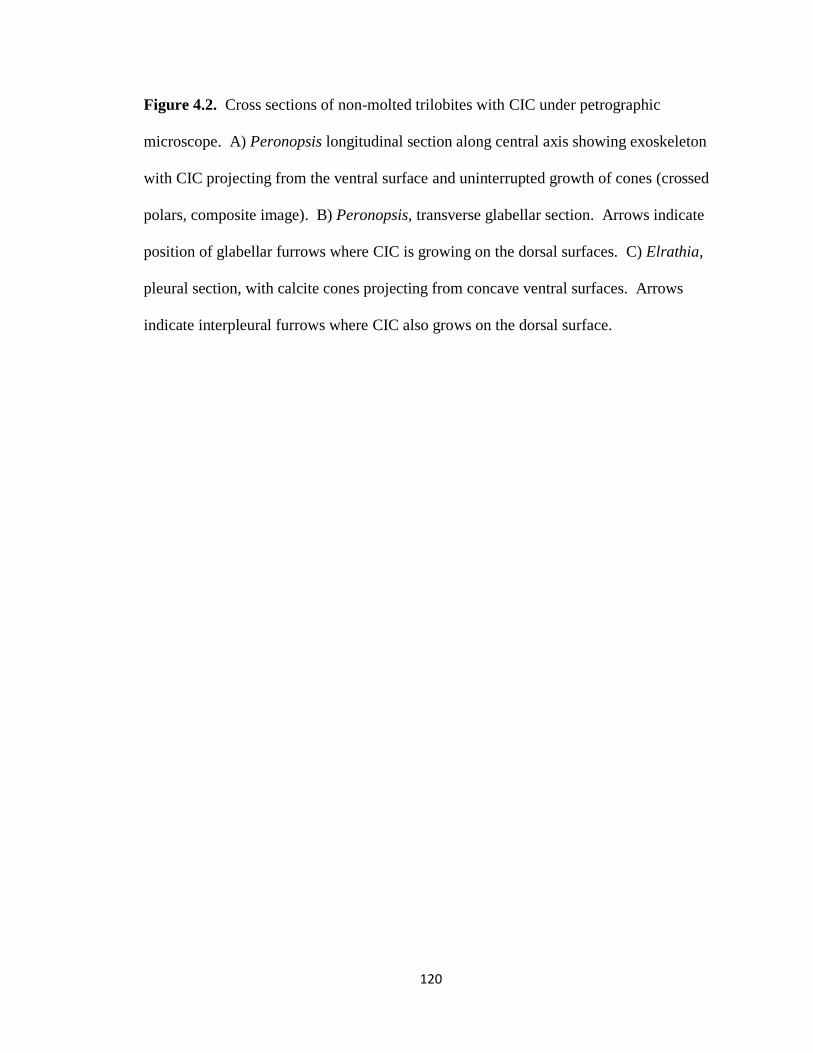
120
Figure 4.2. Cross sections of non-molted trilobites with CIC under petrographic
microscope. A) Peronopsis longitudinal section along central axis showing exoskeleton
with CIC projecting from the ventral surface and uninterrupted growth of cones (crossed
polars, composite image). B) Peronopsis, transverse glabellar section. Arrows indicate
position of glabellar furrows where CIC is growing on the dorsal surfaces. C) Elrathia,
pleural section, with calcite cones projecting from concave ventral surfaces. Arrows
indicate interpleural furrows where CIC also grows on the dorsal surface.

121

122
Figure 4.3. Disarticulated sclerite fragments buried alongside Peronopsis under
petrographic microscope. Cone-in-cone growth is considerably thinner than non-molted
trilobites. A) Sclerite with bottom-only CIC growth. B) Sclerite with top-and-bottom
CIC growth.
4
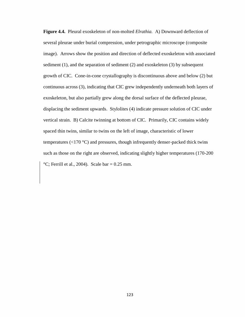
123
Figure 4.4. Pleural exoskeleton of non-molted Elrathia. A) Downward deflection of
several pleurae under burial compression, under petrographic microscope (composite
image). Arrows show the position and direction of deflected exoskeleton with associated
sediment (1), and the separation of sediment (2) and exoskeleton (3) by subsequent
growth of CIC. Cone-in-cone crystallography is discontinuous above and below (2) but
continuous across (3), indicating that CIC grew independently underneath both layers of
exoskeleton, but also partially grew along the dorsal surface of the deflected pleurae,
displacing the sediment upwards. Stylolites (4) indicate pressure solution of CIC under
vertical strain. B) Calcite twinning at bottom of CIC. Primarily, CIC contains widely
spaced thin twins, similar to twins on the left of image, characteristic of lower
temperatures (<170 °C) and pressures, though infrequently denser-packed thick twins
such as those on the right are observed, indicating slightly higher temperatures (170-200
°C; Ferrill et al., 2004). Scale bar = 0.25 mm.
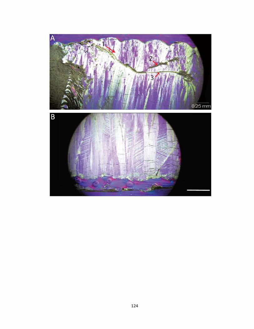
124
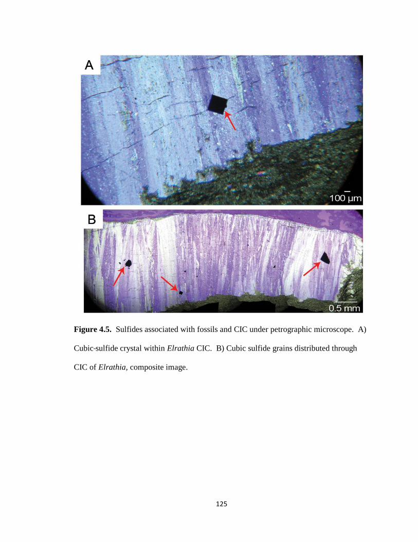
125
Figure 4.5. Sulfides associated with fossils and CIC under petrographic microscope. A)
Cubic sulfide crystal within Elrathia CIC. B) Cubic sulfide grains distributed through
CIC of Elrathia, composite image.
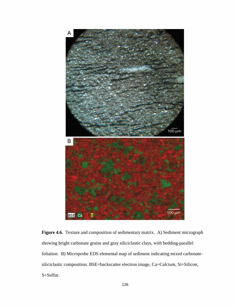
126
Figure 4.6. Texture and composition of sedimentary matrix. A) Sediment micrograph
showing bright carbonate grains and gray siliciclastic clays, with bedding-parallel
foliation. B) Microprobe EDS elemental map of sediment indicating mixed carbonate-
siliciclastic composition. BSE=backscatter electron image, Ca=Calcium, Si=Silicon,
S=Sulfur.

127
Figure 4.7. Deformation of sediment around fossil margins of Elrathia under
petrographic microscope. A, B) Cone-in-cone intergrown with nearby compacted and
cohesive sediment, which is deflected downward by CIC growth. Foliations remain
distinct where deformed, indicating cohesive deformation of the sediment. Cone-in-cone
beds intergrown with sedimentary layers suggest growth is mediated by low-pressure
zones where shearing created vertical extension, reducing stress from compaction.
Specimen figured in A) is same as in Fig. 4.4A and contains the microstylolites described
there, indicating pressure dissolution of CIC carbonate in response to vertical strain.
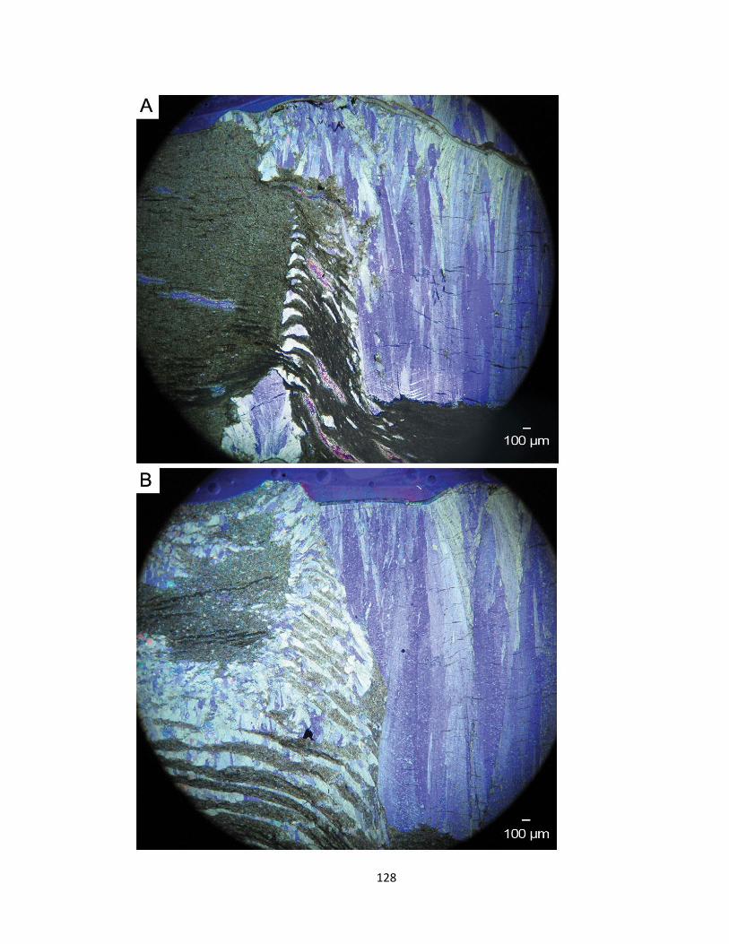
128

129
Figure 4.8. Graphical depiction of data in Table 4.1. Weight percentages of Ca, Mg, S, and Fe for each sample type: whole
Peronopsis exoskeletons, molted and whole Elrathia kingii exoskeletons, CIC, and sediment. Sulfur values were at or below
detection limits for most specimens.

130
Figure 4.9. Silicification of exoskeletal calcite. BSE=backscatter electron image, Ca=Calcium,
Si=Silicon, S=Sulfur. A) Elrathia thoracic pleurae and deflected exoskeleton within CIC,
photomicrograph. Arrows point to exoskeleton along surface (1), and inclusions of silicon-rich
sediment within CIC structure (2-3). B) Microprobe EDS elemental map of area in A. Partially
silicified exoskeleton and sediment inclusions are distinct from calcium in exoskeleton and CIC.
C) Peronopsis, glabellar section, photomicrograph. Arrow points to exoskeleton between layers
of CIC along glabellar furrow. D) Microprobe EDS elemental map of area in C. Exoskeleton is
partially silicified between layers of CIC.

131

132
Figure 4.10. Carbon and calcium distributions under ESEM EDS elemental map. For both Peronopsis and Elrathia, carbon
concentration does not appear to represent any soft tissue structures, but appears wherever carbonate exoskeleton, as indicated
by the Ca distribution, is exposed.
133
Figure 4.11. Schematic of preservational pathway in Wheeler Shale. A) Life position. Elrathia
inhabits the benthos while Peronopsis is pelagic. B) Post death and early diagenesis, a trilobite
exoskeleton is buried, but conditions are not yet sulfur-reducing. C) Late diagenesis, compaction
and heating begin, generating laminations in the sediment. The sediment becomes cohesive, but
remains plastic. Bacterial sulfate reduction commences, forming cubic pyrite. D) Sulfate
reduction has generated enough alkalinity to reach supersaturation. Porewaters diffuse upwards
into carapace, concentrating and nucleating CIC along the ventral surface. Some nucleation may
also occur on the dorsal surface. Exoskeleton recrystallizes to diagenetic calcite. E) Cone-in-
cone continues to grow downward, displacing sediment layers. Additional CIC grows between
displaced sediment layers where pressure from compaction is relieved. Pyrite inclusions become
entrained in CIC. F) Late diagenesis to low-grade metamorphism. Compaction continues to
compress trilobites, generating brittle fractures and microstylolites in CIC perpendicular to
strain. Sediment becomes more lithified. G) Recent weathering. Oxic meteoric groundwater
weathers the sediment, oxidizing any sedimentary pyrite. Inclusions of pyrite remain protected.
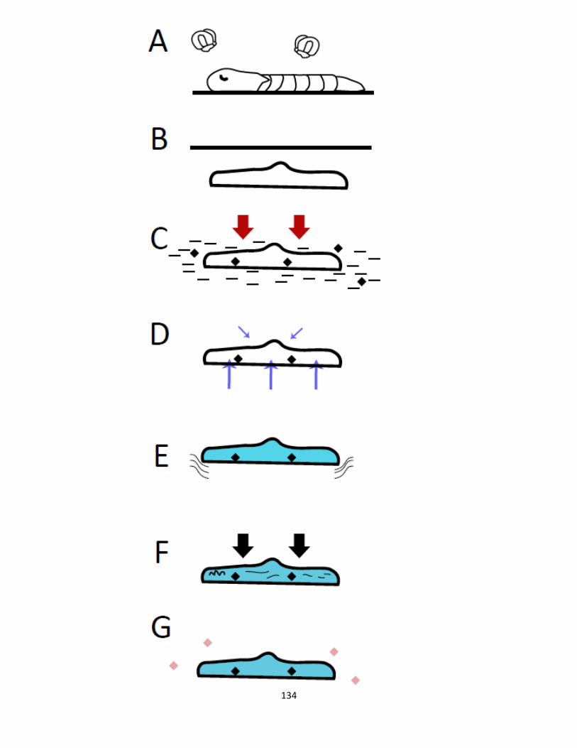
134

135
Table 4.1. Mean elemental weight percentages for different sample types under
microprobe WDS analysis. Ca, Mg, Fe, and S average values are given for Peronopsis
exoskeletons and associated CIC and sediment, for Elrathia kingii molted and whole specimens
with associated CIC and sediment and for all Elrathia exoskeletons combined, and for total CIC
and sediment from all sources combined. Precisions were ±0.04 for Ca, ±<0.01 for Mg, ±0.06
for Fe, and ±0.01 for S. Detection limits were 0.03 wt. % for Ca, 0.03 for Mg, 0.11 for Fe, and
0.01 for S. Original data tabulated in Appendix 4.1.
Sample type Ca Mg Fe S
Peronopsis
total exoskeleton 38.37 0.31 0.59 0.01
cone-in-cone 39.49 0.12 0.25 0.00
sediment 29.43 0.35 0.54 0.03
Elrathia molts
exoskeleton, molts 35.90 0.63 0.39 0.02
cone-in-cone, molts 40.74 0.11 0.22 0.01
sediment, molts 6.09 2.16 2.83 0.01
Elrathia whole
exoskeleton 31.46 0.49 0.45 0.01
cone-in-cone 34.78 0.21 0.30 0.00
sediment 0.07 0.47 0.83 0.00
Elrathia total exoskeleton 33.57 0.56 0.42 0.01
Total exoskeleton 34.90 0.49 0.47 0.01
Total cone-in-cone 37.45 0.16 0.27 0.00
Total sediment 12.87 1.27 1.73 0.01

136
CHAPTER 5
CONSTRAINING OXYGEN AND SULFIDE LEVELS IN CAMBRIAN WHEELER
SHALE SEDIMENTS1
___________
1 John, D. J. and Walker, S. E. To be submitted to Geology.

137
Abstract
Trilobites from the middle Cambrian Wheeler Shale of Utah have excellent preservation
and unusual modes of life tied to distinctive sedimentological and chemical conditions.
These conditions included fluctuations of oxygen levels in the benthos, driving distinct
taphofacies for oxic, dysoxic, and anoxic conditions. Trilobites such as Elrathia kingii
were interpreted to bear special adaptations for inhabiting dysoxic habitats, including
potential symbiosis with sulfur-reducing bacteria. However, though it plays a large role
in determining the life habits and preservation of benthic organisms, the oxygenation of
the benthos has not been constrained through direct geochemical analyses. Here, we
perform a suite of geochemical analyses targeting iron (Fe), sulfur (S), carbon (C), and
trace metals such as chromium (Cr), vanadium (V), uranium (U), and molybdenum (Mo)
to better constrain the presence of dysoxic benthic conditions in putatively dysoxic
horizons containing abundant E. kingii and Peronopsis interstricta and few other species.
We found that the geochemistry of these sediments does not support extreme dysoxia or
free sulfide above the sediment-water interface. Iron was not extensively scavenged by
sulfides, as it would be under euxinic conditions. The euxinia-sensitive trace metals Mo
and U were not enriched above detrital values, indicating no free sulfide, but the anoxia-
sensitive trace metals Cr and V were enriched, indicating reduced oxygen levels.
Elrathia may have simply tolerated lower oxygen conditions than other benthic trilobites
and, from previous work, was likely not symbiotic with sulfate-reducing bacteria. Our
findings suggest that, within the dysoxic horizons examined, the ecology and
preservation of organisms in the Wheeler Shale is not driven by exceptionally low-
oxygen or euxinic conditions.

138
Introduction
The middle Cambrian Wheeler Shale of Utah is host to a famous and important
trilobite Lagerstätte that includes the famous trilobite Elrathia kingii. Fossils exhibit
several unusual and exceptional modes of preservation, including Burgess-Shale type
preservation sediments, as well as cone-in-cone calcite (CIC) encrustations. The
exceptional preservation in the Wheeler Shale has long been associated with dysoxia in
the benthos (Bright, 1959; Rees, 1986) and drawn comparison to similar preservational
pathways for the Burgess Shale (Halgedahl et al., 2009). The CIC encrustations that help
enhance preservation are thought to be related to sulfur-reducing microenvironments
contained within buried trilobite exoskeletons (Gaines et al., 2005). Likewise, Elrathia
has been interpreted as a specialist for these exaerobic conditions, possibly through an
association with sulfur-oxidizing bacterial symbionts (Gaines and Droser, 2003).
However, an examination of the morphological basis for that interpretation suggested that
Elrathia is not symbiotic (John and Walker, 2016). Trilobites occur within several
taphofacies, thought to be controlled by changes in oxygen levels, with horizons
containing high-abundance, low diversity assemblages of E. kingii and the smaller
agnostid trilobite Peronopsis interstricta representing extreme low-oxygen environments
(Gaines et al., 2005). However, the degree to which their habitats were dysoxic remains
to be constrained. Oxygen conditions of the benthos have been interpreted using
sedimentological and ichnofabric data, and isotopic sulfur analysis suggests fluctuations
in bacterial sulfate reduction (Gaines et al., 2012). However, the sediments have not been
directly tested for geochemical evidence of low-oxygen conditions. Here, we determine
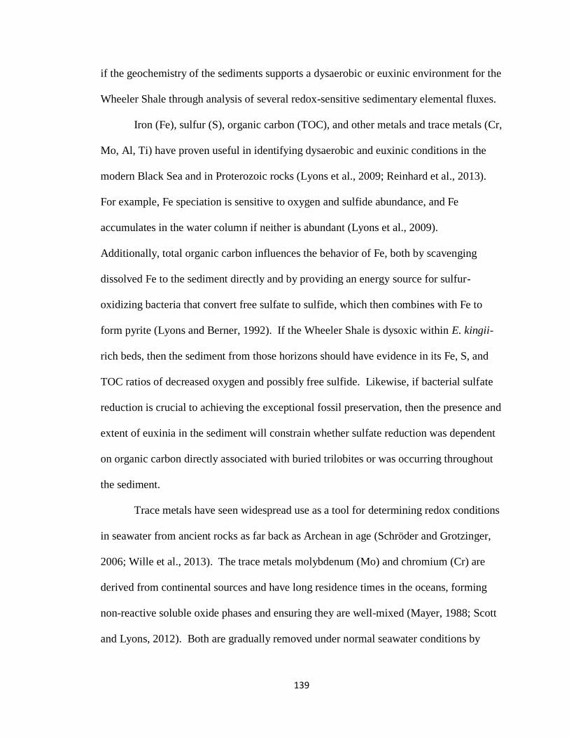
139
if the geochemistry of the sediments supports a dysaerobic or euxinic environment for the
Wheeler Shale through analysis of several redox-sensitive sedimentary elemental fluxes.
Iron (Fe), sulfur (S), organic carbon (TOC), and other metals and trace metals (Cr,
Mo, Al, Ti) have proven useful in identifying dysaerobic and euxinic conditions in the
modern Black Sea and in Proterozoic rocks (Lyons et al., 2009; Reinhard et al., 2013).
For example, Fe speciation is sensitive to oxygen and sulfide abundance, and Fe
accumulates in the water column if neither is abundant (Lyons et al., 2009).
Additionally, total organic carbon influences the behavior of Fe, both by scavenging
dissolved Fe to the sediment directly and by providing an energy source for sulfur-
oxidizing bacteria that convert free sulfate to sulfide, which then combines with Fe to
form pyrite (Lyons and Berner, 1992). If the Wheeler Shale is dysoxic within E. kingii-
rich beds, then the sediment from those horizons should have evidence in its Fe, S, and
TOC ratios of decreased oxygen and possibly free sulfide. Likewise, if bacterial sulfate
reduction is crucial to achieving the exceptional fossil preservation, then the presence and
extent of euxinia in the sediment will constrain whether sulfate reduction was dependent
on organic carbon directly associated with buried trilobites or was occurring throughout
the sediment.
Trace metals have seen widespread use as a tool for determining redox conditions
in seawater from ancient rocks as far back as Archean in age (Schröder and Grotzinger,
2006; Wille et al., 2013). The trace metals molybdenum (Mo) and chromium (Cr) are
derived from continental sources and have long residence times in the oceans, forming
non-reactive soluble oxide phases and ensuring they are well-mixed (Mayer, 1988; Scott
and Lyons, 2012). Both are gradually removed under normal seawater conditions by

140
complexing with Fe or manganese (Mn) oxyhydroxides, generating detrital fluxes
comparable to crustal concentrations (Tribovillard et al., 2006). They can be used
together to constrain oxygen levels because they are strongly redox-sensitive under
different conditions: Mo is scavenged nearly quantitatively from solution exclusively
under euxinic conditions, where it converts from non-reactive molybdate to a series of
reactive thiomolybdates that form ligands with Fe- or S-rich particles and iron sulfides
(Tribovillard et al., 2006). A similar behavior is observed for uranium (U), where U(VI)
under oxic conditions is reduced to U(IV) in the presence of sulfide, adsorbing and
scavenging to the sediment (Tribovillard et al., 2006). Conversely, Cr transitions from
soluble, nonreactive Cr(IV) in chromate to reactive Cr(III) under anoxic conditions, and
is scavenged by organic particles or Fe- or Mn-oxyhydroxides (Tribovillard et al., 2006).
Thus Cr becomes enriched in the sediment under either anoxic or euxinic conditions
(Tribovillard et al., 2006). Another trace metal behaving in this manner is vanadium (V),
which also enriches under anoxic conditions, though it is slightly less sensitive to
reductions in oxygen than Cr (Schröder and Grotzinger, 2006). An enrichment of all
trace metals above background detrital levels suggests euxinia, an enrichment of only Cr
and V suggests anoxia, while enrichment of Cr but not V suggests dysoxia, and oxic
conditions can be inferred where none is enriched (Tribovillard et al., 2006; Lyons et al.,
2003; 2009). Additionally, concentrations of Mo indicate the degree of euxinia. Under
fully euxinic conditions in the water column (H2S > ~100 μM), Mo is enriched hundreds
of times higher than crustal input values (Lyons et al. 2003). Under dysaerobic
conditions with low-oxygen waters overlying sulfidic pore waters in the sediment (H2S >
0 μM), Mo is enriched only on the order of ten times higher than crustal input (Lyons et

141
al., 2003). While Mo and U concentrations can be interpreted directly, Cr and V
enrichments are first normalized to the detrital flux by using their ratio with a detrital
proxy element such as Ti. If the Wheeler Shale benthos are euxinic, then all trace metals
should be enriched, indicating reduced oxygen levels and free sulfide in either the
underlying sediment or the water column. If only Cr and V are enriched, that suggests
bottom-water dysoxia but no free sulfide. If no trace metals are enriched in the
sediments, then benthic conditions were more oxic and the ecology of Elrathia may not
be exclusively dysaerobic.
Methods
Five tests were performed to examine the geochemistry of the Wheeler Shale
sediment: 1) total carbon/total sulfur analysis, to give baseline values used to compare to
organic carbon and pyrite sulfur; 2) total inorganic carbon analysis that when subtracted
from total carbon yields organic carbon, which influences Fe and S cycles; 3) chromium
reduction, to quantify the amount of pyrite; 4) sequential iron reduction, to quantify the
amount of reactive Fe; and 5) total metal digest, to quantify the concentrations of metals
such as Fe, aluminum (Al) and Ti, and trace metals. All sample preparation and analysis
was performed at the Lyons Geochemistry Lab, UC Riverside, California (USA).
Twenty-five samples of sediment from the Wheeler Shale were used for the five
analyses. Samples were collected by professional collectors from freshly-exposed
outcrops buried under ~ five meters of overburden. Each sample was associated with a
trilobite; 18 were associated with E. kingii, and 7 were associated with P. interstricta.
These two species make up the preponderance of the dysoxic assemblage (Gaines et al.,

142
2005), and both were included in the analysis to control for any possible preservational
bias for Elrathia. Trilobites with CIC were separated from the sediment using tungsten
carbide-coated hand chisels, and sediment immediately underlying the fossil was isolated
by breaking away adjacent sediment with a rock hammer (Fig. 5.1). The underlying
sediment, which had not been in contact with steel tools, was then pulverized in a Spex
8000 mill with an aluminum ceramic grinding ball to yield approximately 20 ml of
powder for each sample. Each powdered sample was subdivided for the five tests.
For the total carbon/total sulfur analysis, ~100 mg of sample powder was weighed
into a crucible and fired on an Eltra furnace to approximately 1350 °C under a pure
oxygen atmosphere. All C and S in the sample was converted to CO2 and SO2 gas,
respectively, which was measured by infrared absorption on an Eltra CS500 determinator
to yield total weight percent C and S in the sample. An Alpha Resources AR4007 ore
standard was run six times before and twice after samples, and indicated a precision of
±1.8% for C and ±18.3% for S.
For the total inorganic carbon (TIC) analysis, sample powder (~100 mg) was
weighed into a 250 ml flask and mixed with ethanol (~10 ml) to suspend the powder.
The flask was connected to an Eltra CS500 determinator, 20% HCl (~10 ml) was added,
and the mixture heated to ~50 °C to convert all inorganic carbon to CO2. The CO2 was
measured to yield weight percent inorganic carbon. Weight percent of organic carbon
was then determined as the difference between total and inorganic carbon. An Alpha
Resources AR 4007 was run three times before and once after the samples, and indicated
a precision of ±3.6% for C and ±5.5% for S.
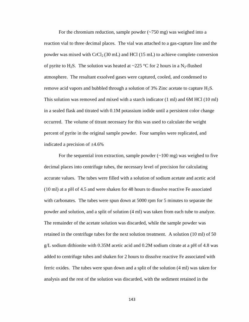
143
For the chromium reduction, sample powder (~750 mg) was weighed into a
reaction vial to three decimal places. The vial was attached to a gas-capture line and the
powder was mixed with CrCl2 (30 mL) and HCl (15 mL) to achieve complete conversion
of pyrite to H2S. The solution was heated at ~225 °C for 2 hours in a N2-flushed
atmosphere. The resultant exsolved gases were captured, cooled, and condensed to
remove acid vapors and bubbled through a solution of 3% Zinc acetate to capture H2S.
This solution was removed and mixed with a starch indicator (1 ml) and 6M HCl (10 ml)
in a sealed flask and titrated with 0.1M potassium iodide until a persistent color change
occurred. The volume of titrant necessary for this was used to calculate the weight
percent of pyrite in the original sample powder. Four samples were replicated, and
indicated a precision of ±4.6%
For the sequential iron extraction, sample powder (~100 mg) was weighed to five
decimal places into centrifuge tubes, the necessary level of precision for calculating
accurate values. The tubes were filled with a solution of sodium acetate and acetic acid
(10 ml) at a pH of 4.5 and were shaken for 48 hours to dissolve reactive Fe associated
with carbonates. The tubes were spun down at 5000 rpm for 5 minutes to separate the
powder and solution, and a split of solution (4 ml) was taken from each tube to analyze.
The remainder of the acetate solution was discarded, while the sample powder was
retained in the centrifuge tubes for the next solution treatment. A solution (10 ml) of 50
g/L sodium dithionite with 0.35M acetic acid and 0.2M sodium citrate at a pH of 4.8 was
added to centrifuge tubes and shaken for 2 hours to dissolve reactive Fe associated with
ferric oxides. The tubes were spun down and a split of the solution (4 ml) was taken for
analysis and the rest of the solution was discarded, with the sediment retained in the
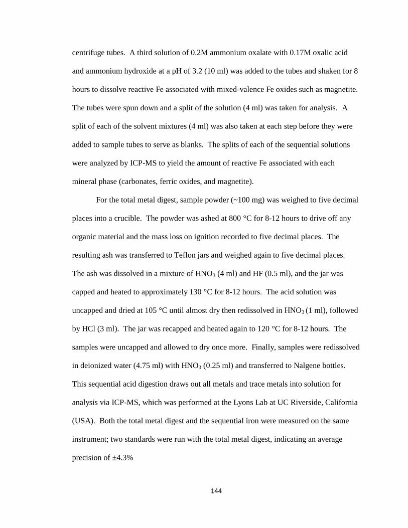
144
centrifuge tubes. A third solution of 0.2M ammonium oxalate with 0.17M oxalic acid
and ammonium hydroxide at a pH of 3.2 (10 ml) was added to the tubes and shaken for 8
hours to dissolve reactive Fe associated with mixed-valence Fe oxides such as magnetite.
The tubes were spun down and a split of the solution (4 ml) was taken for analysis. A
split of each of the solvent mixtures (4 ml) was also taken at each step before they were
added to sample tubes to serve as blanks. The splits of each of the sequential solutions
were analyzed by ICP-MS to yield the amount of reactive Fe associated with each
mineral phase (carbonates, ferric oxides, and magnetite).
For the total metal digest, sample powder (~100 mg) was weighed to five decimal
places into a crucible. The powder was ashed at 800 °C for 8-12 hours to drive off any
organic material and the mass loss on ignition recorded to five decimal places. The
resulting ash was transferred to Teflon jars and weighed again to five decimal places.
The ash was dissolved in a mixture of HNO3 (4 ml) and HF (0.5 ml), and the jar was
capped and heated to approximately 130 °C for 8-12 hours. The acid solution was
uncapped and dried at 105 °C until almost dry then redissolved in HNO3 (1 ml), followed
by HCl (3 ml). The jar was recapped and heated again to 120 °C for 8-12 hours. The
samples were uncapped and allowed to dry once more. Finally, samples were redissolved
in deionized water (4.75 ml) with HNO3 (0.25 ml) and transferred to Nalgene bottles.
This sequential acid digestion draws out all metals and trace metals into solution for
analysis via ICP-MS, which was performed at the Lyons Lab at UC Riverside, California
(USA). Both the total metal digest and the sequential iron were measured on the same
instrument; two standards were run with the total metal digest, indicating an average
precision of ±4.3%
145
The first four tests combine to yield data to compare C (both inorganic and
organic), S, and Fe, including the proportion of Fe and S from pyrite; pyrite Fe is added
to the sequential iron extraction’s three Fe concentrations to yield highly reactive Fe
(FeHR). The fifth test yields metal and trace metal concentrations that can be directly
interpreted as well as compared to the results from the first four tests.
Several ratios that give information about paleoenvironmental conditions were
calculated for each sample from the results of these tests. First, the ratio of pyrite sulfur
to total organic carbon (Spy/TOC) indicates euxinic bottom waters. Under oxic
conditions, pyrite formation is linked to the abundance of organic carbon that drives
bacterial sulfate reduction after burial, while under euxinic conditions, pyrite formation is
instead limited by Fe availability, generating much more sedimentary pyrite and thus
Spy/TOC ratios well above the expected Cambrian marine average of ~0.67 (Berner and
Raiswell, 1983). Second, three ratios describe the activity of free sulfide in the water
column (i.e., euxinia). Under euxinic conditions, dissolved Fe is converted to pyrite and
deposited in the sediment, enriching it with highly reactive pyrite Fe relative to the flux
of all iron to the sediment (FeHR/FeT). Ratio values of ~0.6 – 0.7 are characteristic of
euxinic basins, while values of ~0.26 are characteristic of oxic sediments (Lyons and
Severmann, 2006). The total flux of iron is also enriched relative to the rate of
sedimentation (FeT/Al), with euxinic ratios ranging no lower than ~0.6 (Lyons and
Severmann, 2006) and average shale values ~0.5 (Taylor and McLennan, 1985). The
amount of reactive iron deposited as pyrite is enriched relative to the flux of reactive iron
from non-pyrite phases (degree of pyritization, or DOP, calculated as Fepy/FeHR), with
values under 0.42 corresponding to oxic conditions, values above 0.42 representing

146
dysoxic conditions with euxinic porewaters, and values over 0.55 representing fully
euxinic conditions, where the overlap represents gradation between the latter two
(Raiswell et al., 1988; Lyons et al., 2009).
Among the trace metals, the ratio of Cr/Ti describes the enrichment of Cr relative
to detrital sedimentation rate (which gives a ratio roughly equivalent to crustal ratios of
~0.017). Enrichment above background rates (up to ~0.025) indicates anoxic conditions
where Cr scavenging by organic matter is enhanced, while enrichment at background
rates shows that no scavenging is occurring, indicating oxic conditions (Reinhard et al.,
2013). Similarly, V under sufficiently anoxic conditions will enrich beyond its crustal
background rate of ~20 ppm (Schröder and Grotzinger, 2006). Concentrations of Mo
vary strongly by redox conditions, with oxic waters only depositing detrital Mo at
concentrations similar to crustal values of 1-2 ppm. Weakly dysoxic bottom waters
overlying anoxic porewaters scavenge Mo across the sediment-water interface and enrich
Mo to ~20 ppm. Intermittently euxinic waters scavenge directly from the water column
and can enrich to ~60 ppm (Lyons et al., 2009). Concentrations of U follow a similar
pattern to Mo, with non-euxinic conditions depositing at the crustal value of ~2 ppm and
euxinic conditions concentrating upwards of ~10 ppm (Wille et al., 2013). Additionally,
Mo scavenging is linked to abundance of TOC under euxinic conditions, where more
TOC generates more sulfide production and thus more Mo scavenging. Under oxic
conditions, though, Mo scavenging is tied to Mn oxyhydroxide formation, which is
unrelated to TOC. Mo and TOC should therefore show a positive correlation under
euxinic conditions, and no correlation under oxic conditions (Lyons et al., 2009).

147
Measurements of C, S, Fe, Mo, Cr, U, V, aluminum (Al) and titanium (Ti) were
made for each of 25 samples, and means among the samples calculated for each
measurement (Table 5.1; Appendices 5.1-5.5). From these, five ratios were calculated,
along with their means for the 25 samples (Table 5.2).
Results
Variations within measurements
Total carbon ranged from 2.63 – 6.73 wt. %, with a mean of 3.91 wt. %, while
TOC varied proportionally more, from 0.01 – 2.01 wt. % (Table 5.1). A single TOC
measurement of 4.40%, nearly equal to the total carbon measured in Sample 16, is likely
a measurement error, and an unusually low TOC measured in Sample 3 (0.01) potentially
is as well. Ignoring those outliers, the remaining 24 samples have a mean of 0.41 wt. %
organic carbon, comparable to TOC values of ~0.2% in the Burgess Shale (Butterfield,
1995) but less than those reported for the Chengjiang (up to 1.4%; Zhu et al., 2005) or
black shales (up to 10%, Kennedy et al., 2002). Measurements for S and Fe were more
consistent, as were concentrations for Al, Ti, and Cr. The two proxies for anoxia, V and
Cr, corresponded tightly with each other, as did Al and Ti, the two proxies for detrital
flux. However, Mo showed a decreasing pattern from the first nine samples (mean 5.23
ppm) through the last 16 (mean 1.15 ppm). However, the order of samples was random
and this decrease does not correspond to any environmental gradient or difference
between species; it may represent an error in the instrument or may simply be
coincidental. Uranium, the counterpart to Mo as euxinic proxies, varied very little
throughout the samples.

148
These raw values were used to calculate ratios that can indicate seawater
conditions (Table 5.2). While data were generally consistent, a few abnormally high
outliers were identified among TOC (3 samples for TOC ≥1.92 , where all others were
≤0.45) and Mo (Two samples ≥9.83, where all others range between 0.85-5.18). These
are likely measurement errors, given the low concentration of TOC relative to TIC, and
low absolute concentrations of Mo. Ignoring these TOC outliers, Spy/TOC ratios ranged
between 0.03 – 1.32, with a mean of 0.50 (Table 5.3). Ratios of FeHR/FeT varied from
0.18 – 0.47, with a mean of 0.30. Ratios of FeT/Al varied from 0.32 – 0.66, with a mean
of 0.43. Measurements of DOP ranged between 0.02 and 0.24, with a mean of 0.12. The
ratio of Cr/Ti varied between 0.01 and 0.05, with a mean of 0.03.
Measured and calculated values generally did not vary between Elrathia (n = 18)
and Peronopsis (n = 7), with a few exceptions. Peronopsis were significantly higher for
total carbon (p = 0.032, H = 4.616, df = 1 by Kruskal-Wallis analysis with α = 0.05) but
not TOC (p = 0.154, H = 5.871, df = 1). Elrathia was significantly higher than
Peronopsis for concentrations of Mo (p < 0.001, H = 14.538, df = 1). The lack of
significant difference in all other samples suggests that there are no preservational biases
between the two species, and values calculated for either are representative of the overall
unit.
C-S-Fe variations in geochemical conditions in the Wheeler Shale
Carbon, sulfur, and iron suggest that benthic conditions varied between oxic and
generally slightly euxinic conditions (Table 5.3). Spy/TOC ratios vary across euxinic
threshold value of ~0.67, with five of 23 samples consistent with euxinia (mean = 0.48),

149
when two outliers are excluded. FeHR/FeT values are entirely below the threshold of ~0.6
– 0.7 that would indicate euxinia and closer to the oxic average of ~0.28 (mean = 0.30;
Table 5.2; Fig. 5.2). FeT/Al ratios (mean = 0.43; Fig. 5.2) are close to average shale
values of ~0.5 (Taylor and McLennan, 1985), with only two samples ranging above 0.6
into potentially euxinic values (Lyons and Severmann, 2006; Table 5.3). DOP values
(mean = 0.121; Fig. 5.2) are all well below the threshold of ~0.42 where euxinia in the
subsurface begins (Lyons et al., 2009).
Lack of euxinia in Wheeler Shale based on trace elements
Trace metal analyses suggest limited dysoxia with no euxinia in either bottom
waters or sediments. Low values for Mo were detected in all sediments (mean = 2.62
ppm; Table 5.1; Fig. 5.2), similar to crustal values of 1-2 ppm. Of the 25 samples, five
were above the 95% confidence interval (3.692 ppm) for the sample set, but all were still
well below the expected values for weakly dysoxic bottom waters overlying euxinic
porewaters (~20 ppm) or intermittently euxinic bottom waters (~60 ppm; Lyons et al.,
2009; Fig 5.2). Values for U (mean = 2.43 ppm; Table 5.1) were similar to crustal values
of ~2 ppm and well below the euxinic level of ~10 ppm, confirming the Mo values.
Additionally, after removing five outliers with exceptionally high Mo or TOC readings
and applying a natural-log transformation to correct for non-normality, values for Mo and
TOC yielded a Pearson’s correlation coefficient of r = -0.338; with outliers included, the
correlation is weaker (r = -0.177). The correlation is not significant (p = 0.145; α = 0.05),
indicating no correlation, and thus no euxinia in bottom waters (Fig. 5.3).

150
Cr is consistent with dysoxic seawater where trace metals begin to be scavenged
to the sediment. Ratios of Cr/Ti are at the threshold of ~0.025 characteristic of
Phanerozoic anoxic shales (mean = 0.03; Fig. 5.2) (Reinhard et al 2013). Values for V
(mean = 78.67; Table 5.1) are markedly higher than average crustal values of ~20 ppm,
indicating enrichment and dysoxia, confirming the Cr values.
Discussion
The Wheeler Shale benthos, inhabited by Elrathia, was most likely intermittently
dysoxic and not euxinic. Iron, sulfur, and carbon analyses suggest very limited
generation of pyrite from reactive Fe. The relatively low FeHR/FeT values indicate that
the iron being delivered is not in reactive forms, as it would be if Fe was being scavenged
under euxinic conditions. Rather, the FeT/Al ratios near the crustal average suggest that
most of the iron is detrital, likely in non-reactive forms like iron silicates (Lyons and
Severmann, 2006). Likewise, low DOP values suggest that Fe being scavenged into the
sediment is not in the form of pyrite, indicating that the system is sulfide-limited and thus
not euxinic (Lyons et al., 2009).
Trace metals likewise suggest redox-sensitive ions were not being enriched under
euxinic conditions beyond detrital values, but may have been enriched under dysoxic
conditions. Molybdenum and U were not enriched in the sediments as expected for
persistently euxinic conditions (Tribovillard et al, 2006). Molybdenum levels also did
not suggest euxinia in the sediment under a dysoxic water column (Lyons et al., 2009).
The weakly negative correlation observed between Mo and TOC suggests that Mo
deposition is not linked to the generation of free sulfide (Lyons et al., 2009). Therefore,

151
conditions in the Wheeler Shale were not euxinic. However, Cr/Ti ratios and V
concentrations above crustal values suggest that their deposition in the Wheeler Shale
was enriched by scavenging where dysoxic conditions were driving increased Cr and V
flux to the sediment (Reinhard et al., 2013).
We found that sedimentary geochemistry suggests benthic conditions were
slightly dysoxic, but not exaerobic (extremely dysoxic) as previously described (Gaines
and Droser, 2003). The characteristic Elrathia from horizons we analyzed were thus not
an extremophile species adapted for barely oxygenated conditions. Though dissolved
oxygen levels may not have been low enough to cause a change in redox behavior for
iron, sulfur, or trace metals, oxygenation may have still been reduced sufficiently to
inhibit other benthic species, while Elrathia could tolerate those conditions. However,
the lack of evidence for euxinia suggests that Elrathia did not inhabit conditions where
symbiosis with sulfur-oxidizing bacteria (as described by Fortey, 2000) would be
necessary or possible. This corroborates our findings in previous work that morphologies
like Elrathia’s are not related to symbiosis (John and Walker, 2016).
The Fe, S, and euxinia-sensitive trace metal (i.e., U and Mo) data all indicate that
there is not an active sulfate reduction zone close below the sediment-water interface,
where metals and trace metals could flux from oxic bottom waters to euxinic pore waters
and become fixed and enriched in the sediment. This is surprising, as sulfate-reducing
conditions are necessary for the rapid precipitation of the CIC in the Wheeler Shale
(Gaines et al., 2005). This preservation is thought to be related to extremely localized
geochemical gradients driven by bacterial sulfate reduction of organic matter buried
alongside trilobite exoskeletons, and physically contained within the carapace and by

152
occluded porosity in the sediments (Gaines et al., 2005). Our findings suggest that the
sulfate-reduction zone necessary for precipitating CIC may be much deeper, and not
interacting directly with bottom waters. This would suggest CIC formation does not
occur rapidly after burial, but later in diagenesis, consistent with results from Chapter 4.
Conclusion
The geochemistry of the Wheeler Shale suggests weak dysoxia in the benthos,
and a lack of euxinia in the benthos or the immediate subsurface. Carbon-sulfur-iron
ratios all suggest limited formation of pyrite and sequestration of reactive iron, consistent
with more oxic conditions. Trace metal analyses of Cr and V alongside Mo and U also
suggest a lack of enrichment associated with scavenging by organic matter or sulfides
under anoxic or euxinic conditions, respectively. Even within the sediments, low
pyritization and extremely low Mo concentrations suggest a lack of widespread bacterial
sulfate reduction. These findings stand somewhat at odds with the prevailing
interpretations of the Wheeler Shale benthos, which are thought to be more pervasively
dysoxic with active subsurface sulfate reduction. Our study raises the possibility that
Elrathia may not be an extreme low-oxygen specialist, but merely tolerant of lower
oxygen levels than other benthic trilobites. Likewise, the lack of geochemical evidence
for a widespread, anoxic sulfate-reducing zone in the sediment, despite the presence of
CIC growth on the trilobites that necessitates sulfate reduction, suggests that CIC may be
forming later and slower than previously described. Our results, based on geochemical
signals heretofore unexplored in the Wheeler Shale, bring a new perspective to our
understanding of the ecology and exceptional preservation of its trilobites

153
References
Berner, RA and Raiswell, R. Burial of organic carbon and pyrite sulfur in sediments over
Phanerozoic time: a new theory. Geochimica et Cosmochimica Acta, 47:855-862.
Bright, RC. 1959. A paleoecologic and biometric study of the middle Cambrian trilobite
Elrathia kingii (Meek). Journal of Paleontology, 33:83-98.
Butterfield, NJ. 1995. Secular distribution of Burgess-Shale-type preservation. Lethaia,
28:1-13.
Ferrill, D.A., Morris, A.P., Evans, M.A., Burkhard, M., Groshong, R.H. Jr., and Onasch,
C.M. 2004. Calcite twin morphology: a low-temperature deformation
geothermometer. Journal of Structural Geology Acta, v. 26, p. 1521-1529.
Fortey, R. 2000. Olenid trilobites: the oldest known chemoautotrophic symbionts?
PNAS, 97:6574-6578.
Gaines, RR and Droser, ML. 2003. Paleoecology of the familiar trilobite Elrathia kingii:
an early exaerobic zone inhabitant. Geology, 31:941-944.
Gaines, RR, Kennedy, MJ, and Droser, ML. 2005. A new hypothesis for organic
preservation of Burgess Shale taxa in the middle Cambrian Wheeler Formation,
House Range, Utah. Palaeogeography, Palaeoclimatology, Palaeoecology, 220:193-
205.
Gaines, RR, et al. 2012. Mechanism for Burgess Shale-type preservation. PNAS,
109:5180-5184.
Halgedahl, SL, Jarrard, RD, Brett, CE, and Allison, PA. 2009. Geophysical and
geological signatures of relative sea level change in the upper Wheeler Formation,

154
Drum Mountains, West-Central Utah: A perspective into exceptional preservation of
fossils. Palaeogeography, Palaeoclimatology, Palaeoecology, 277:34-56.
John, DJ and Walker, SE. 2016. Testing symbiotic morphology in trilobites under
dysoxic and oxic conditions from Cambrian to Early Ordovician Lagerstätten.
Palaeogeography, Palaeoclimatology, Palaeoecology, 441:704-720.
Kennedy, MJ, Pevear, DR, and Hill, RJ. 2002. Mineral surface control of organic carbon
in black shale. Science, 295:657-660.
Lyons, TW and Berner, RA. 1992. Carbon-sulfur-iron systematics of the uppermost
deep-water sediments of the Black Sea. Chemical Geology, 99:1-27.
Lyons, TW, and Severmann, S. 2006. A critical look at iron paleoredox proxies: new
insights from modern euxinic marine basins. Geochimica et Cosmochimica Acta,
70:5698-5722.
Lyons, TW, Werne, JP, Hollander, DL, and Murray, RW. 2003. Contrasting sulfur
geochemistry and Fe/Al and Mo/Al ratios across the last oxic-to-anoxic transition in
the Cariaco Basin, Venezuela. Chemical Geology, 195:131-157
Lyons, TW, Anbar, AD, Severmann, S, Scott, C, and Gill, BC. 2009. Tracking euxinia
in the ancient ocean: a multiproxy perspective and proterozoic case study. Annual
Review of Earth and Planetary Science, 37:507-534.
Mayer, J. 1988. Geochemistry of chromium in the oceans. in Chromium in Natural and
Human Environments, JO Nriagu and E Niebor, eds., Wiley.
Raiswell, R, Buckley, F, Berner, RA, and Anderson, TF. 1988. Degree of pyritization of
iron as a paleoenvironmental indicator of bottom-water oxygenation. Journal of
Sedimentary Petrology, 58:812-819
155
Reinhard, CT, Planavsky, NJ, Robbins, LJ, Partin, CA, Gill, BC, Lalonde, SV, Bekker,
A, Konhauser, KO, and Lyons, TW. 2013. Proterozoic ocean redox and
biogeochemical stasis. PNAS, 110:5357-5362.
Rees, MN. 1986. A fault-trough through a carbonate platform: the Middle Cambrian
House Range embayment. GSA Bulletin, 97:1054-1069.
Scott, C and Lyons T. 2012. Contrasting molybdenum cycling and isotopic properties in
euxinic versus non-euxinic sediments and sedimentary rocks: refining the
paleoproxies. Chemical Geology, v. 324-325, p. 19-27.
Taylor, SR, and McLennan, SM. 1985. The Continental Crust: Its Composition and
Evolution. Blackwell, Oxford.
Tribovillard, N, Algeo, TJ, Lyons, T, and Ribolleau, A. 2006. Trace metals as
paleoredox and paleoproductivity proxies: an update. Chemical Geology, 232:12-32.
Wille, M, Nebel, O, Van Kranendonk, MJ, Schoenberg, R, Kleinhanns, IC, and Elwood,
MJ. 2013. Mo-Cr evidence for a reducing Archean atmosphere in 3.4-2.76 Ga black
shales from the Pilbara, Western Australia. Chemical Geology, 340:68-76.
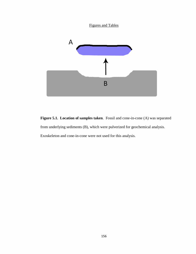
156
Figures and Tables
Figure 5.1. Location of samples taken. Fossil and cone-in-cone (A) was separated
from underlying sediments (B), which were pulverized for geochemical analysis.
Exoskeleton and cone-in-cone were not used for this analysis.
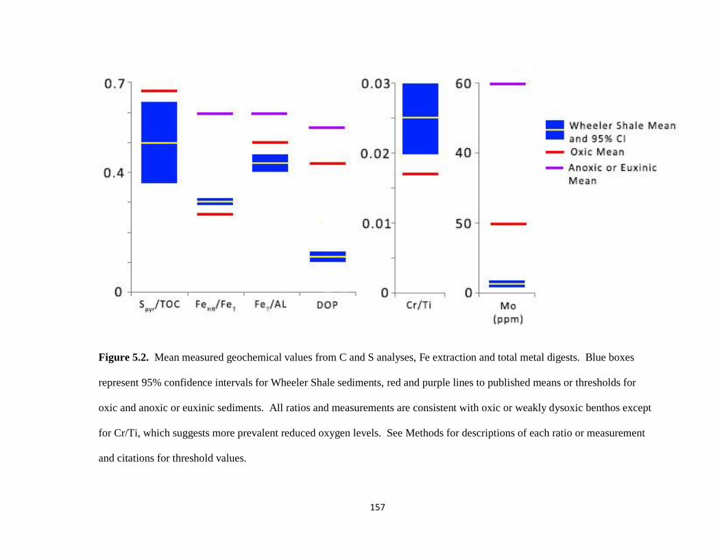
157
Figure 5.2. Mean measured geochemical values from C and S analyses, Fe extraction and total metal digests. Blue boxes
represent 95% confidence intervals for Wheeler Shale sediments, red and purple lines to published means or thresholds for
oxic and anoxic or euxinic sediments. All ratios and measurements are consistent with oxic or weakly dysoxic benthos except
for Cr/Ti, which suggests more prevalent reduced oxygen levels. See Methods for descriptions of each ratio or measurement
and citations for threshold values.

158
Figure 5.3. Total organic carbon (weight %) vs. Mo (ppm) for 20 analyzed specimens. Data have been log-transformed and
outliers have been removed. Dashed line is the regression line, with formula and R2 value. There is no strong positive
correlation between the two elements, as seen in other euxinic localities where organic carbon drives sulfate reduction that
sequesters Mo in the sediment. Molybdenum is thus likely not depositing under euxinia.

159
Table 5.1. Raw data for geochemical analyses. Data for carbon, sulfur, and iron analyses
given in weight percentages: total carbon (TC), total organic carbon (TOC) as calculated by
subtracting inorganic carbon from total carbon, from carbon-sulfur analysis; sulfur from pyrite
(Spy) from chromium reduction analysis; total iron (FeT), highly reactive iron (FeHR), and iron
associated with pyrite (Fepy) from sequential iron extractions, and elemental concentrations from
total metal digests for Al, Mo, Cr, and Ti. Values were averaged by type of fossil associated
with sediments, and overall means were also calculated. Measurements considered potentially
erroneous are marked with an asterisk.

160
Sample
Genus
TC
(wt. %)
TOC
(wt. %)
Spy
(wt. %)
FeT
(wt. %)
FeHR
(wt. %)
Fepy
(wt. %)
1 Elrathia 3.16 0.26 0.135 3.330 0.856 0.118
2 Elrathia 5.84 1.92 0.091 2.612 0.755 0.079
3 Elrathia 3.05 0.01* 0.119 2.240 0.680 0.104
4 Elrathia 3.50 0.12 0.062 2.436 1.011 0.054
5 Elrathia 2.89 0.18 0.160 3.336 0.707 0.139
6 Elrathia 3.21 0.22 0.025 3.161 0.824 0.022
7 Elrathia 2.92 0.32 0.192 1.837 0.863 0.167
8 Elrathia 3.14 0.22 0.189 2.795 0.849 0.165
9 Elrathia 4.30 0.26 0.133 3.184 0.907 0.116
10 Elrathia 2.93 0.19 0.247 2.724 0.699 0.215
11 Elrathia 4.64 2.01 0.060 3.048 0.974 0.052
12 Elrathia 2.63 0.27 0.119 3.065 0.892 0.104
13 Elrathia 6.73 0.20 0.094 2.544 0.652 0.082
14 Elrathia 3.45 0.23 0.149 2.319 0.864 0.130
15 Elrathia 3.06 0.36 0.249 3.149 0.882 0.217
16 Elrathia 4.41 4.40* 0.073 2.441 0.657 0.064
17 Elrathia 3.13 0.16 0.022 2.930 0.888 0.019
18 Elrathia 3.39 0.26 0.235 2.850 0.955 0.205
Mean,
Elrathia 3.69 0.64 0.131 2.778 0.829 0.114
19 Peronopsis 5.20 0.29 0.149 1.748 0.759 0.130
20 Peronopsis 4.75 0.44 0.185 2.779 0.778 0.161
21 Peronopsis 3.16 0.37 0.170 2.347 0.612 0.148
22 Peronopsis 5.12 0.27 0.165 2.814 0.898 0.144
23 Peronopsis 5.25 0.37 0.148 3.127 0.754 0.129
24 Peronopsis 3.98 0.14 0.042 3.364 0.705 0.037
25 Peronopsis 3.87 0.45 0.021 3.611 0.662 0.018
Mean,
Peronopsis 4.48 0.33 0.126 2.827 0.738 0.109
Grand Mean 3.91 0.56 0.13 2.792 0.803 0.113
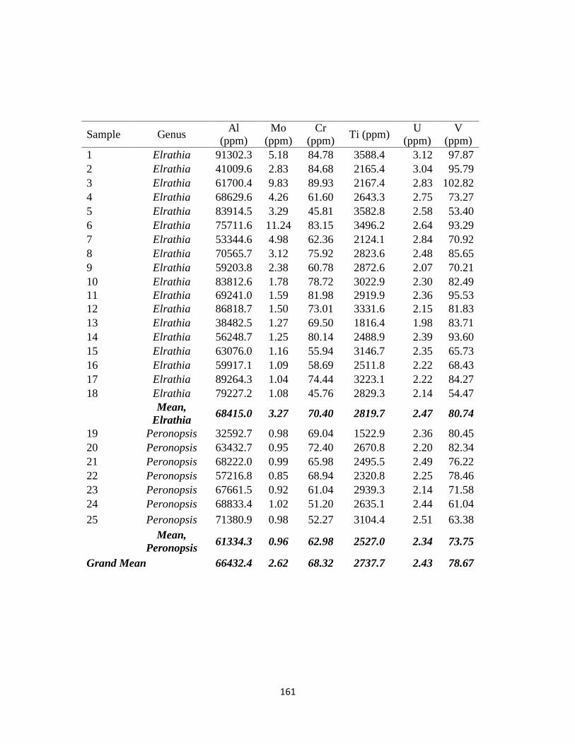
161
Sample Genus Al
(ppm) Mo
(ppm) Cr
(ppm) Ti (ppm)
U (ppm)
V (ppm)
1 Elrathia 91302.3 5.18 84.78 3588.4 3.12 97.87
2 Elrathia 41009.6 2.83 84.68 2165.4 3.04 95.79
3 Elrathia 61700.4 9.83 89.93 2167.4 2.83 102.82
4 Elrathia 68629.6 4.26 61.60 2643.3 2.75 73.27
5 Elrathia 83914.5 3.29 45.81 3582.8 2.58 53.40
6 Elrathia 75711.6 11.24 83.15 3496.2 2.64 93.29
7 Elrathia 53344.6 4.98 62.36 2124.1 2.84 70.92
8 Elrathia 70565.7 3.12 75.92 2823.6 2.48 85.65
9 Elrathia 59203.8 2.38 60.78 2872.6 2.07 70.21
10 Elrathia 83812.6 1.78 78.72 3022.9 2.30 82.49
11 Elrathia 69241.0 1.59 81.98 2919.9 2.36 95.53
12 Elrathia 86818.7 1.50 73.01 3331.6 2.15 81.83
13 Elrathia 38482.5 1.27 69.50 1816.4 1.98 83.71
14 Elrathia 56248.7 1.25 80.14 2488.9 2.39 93.60
15 Elrathia 63076.0 1.16 55.94 3146.7 2.35 65.73
16 Elrathia 59917.1 1.09 58.69 2511.8 2.22 68.43
17 Elrathia 89264.3 1.04 74.44 3223.1 2.22 84.27
18 Elrathia 79227.2 1.08 45.76 2829.3 2.14 54.47
Mean,
Elrathia 68415.0 3.27 70.40 2819.7 2.47 80.74
19 Peronopsis 32592.7 0.98 69.04 1522.9 2.36 80.45
20 Peronopsis 63432.7 0.95 72.40 2670.8 2.20 82.34
21 Peronopsis 68222.0 0.99 65.98 2495.5 2.49 76.22
22 Peronopsis 57216.8 0.85 68.94 2320.8 2.25 78.46
23 Peronopsis 67661.5 0.92 61.04 2939.3 2.14 71.58
24 Peronopsis 68833.4 1.02 51.20 2635.1 2.44 61.04
25 Peronopsis 71380.9 0.98 52.27 3104.4 2.51 63.38
Mean,
Peronopsis 61334.3 0.96 62.98 2527.0 2.34 73.75
Grand Mean 66432.4 2.62 68.32 2737.7 2.43 78.67

162
Table 5.2. Calculated ratios for elemental data indicating environmental
conditions. Ratio of S as pyrite to total organic carbon (Spy/TOC), highly reactive to
total Fe (FeHR/FeT), total Fe to Al (FeT/Al), Cr to Ti, and degree of pyritization (DOP),
calculated as Fepy/(Fepy+FeHR). Ratios were averaged by type of fossil associated with
sediments, and overall means were also calculated. Measurements considered potentially
erroneous are marked with an asterisk.
Sample Genus Spy/TOC FeHR/FeT FeT/Al DOP Cr/Ti
1 Elrathia 0.52 0.257 0.36 0.121 0.024
2 Elrathia 0.05 0.289 0.64 0.095 0.039
3 Elrathia 9.88* 0.303 0.36 0.132 0.041
4 Elrathia 0.51 0.415 0.36 0.051 0.023
5 Elrathia 0.88 0.212 0.40 0.165 0.013
6 Elrathia 0.11 0.261 0.42 0.026 0.024
7 Elrathia 0.60 0.470 0.34 0.162 0.029
8 Elrathia 0.87 0.304 0.40 0.162 0.027
9 Elrathia 0.51 0.285 0.54 0.113 0.021
10 Elrathia 1.32 0.257 0.32 0.235 0.026
11 Elrathia 0.03 0.320 0.44 0.051 0.028
12 Elrathia 0.44 0.291 0.35 0.104 0.022
13 Elrathia 0.47 0.256 0.66 0.112 0.038
14 Elrathia 0.65 0.372 0.41 0.131 0.032
15 Elrathia 0.69 0.280 0.50 0.197 0.018
16 Elrathia 0.02* 0.269 0.41 0.088 0.023
17 Elrathia 0.14 0.303 0.33 0.021 0.023
18 Elrathia 0.91 0.335 0.36 0.177 0.016
Mean,
Elrathia 1.03 0.304 0.42 0.119 0.026
19 Peronopsis 0.52 0.434 0.54 0.146 0.045
20 Peronopsis 0.42 0.280 0.44 0.172 0.027
21 Peronopsis 0.46 0.261 0.34 0.195 0.026
22 Peronopsis 0.61 0.319 0.49 0.138 0.030
23 Peronopsis 0.40 0.241 0.46 0.146 0.020
24 Peronopsis 0.31 0.210 0.49 0.049 0.019
25 Peronopsis 0.05 0.183 0.51 0.027 0.017
Mean,
Peronopsis 0.39 0.275 0.47 0.125 0.027
Grand Mean 0.85 0.296 0.43 0.121 0.026

163
CHAPTER 6
CONCLUSIONS
My work suggests that the environments inhabited by Elrathia and Peronopsis
were not extremely dysoxic. Thus, the role that trilobites such as Elrathia and
Peronopsis played in the ecology of that benthos does not appear to be symbiotic, as
previously suggested based on their similar morphology to olenid trilobites.
Morphological analysis for a wide set of Cambrian trilobites suggests that a
similarity to olenids is not related to low-oxygen conditions, as would be expected if the
morphology was an adaptation to facilitate symbiosis. Rather, it seems that the
morphology is common among ptychopariid trilobites from all environments, suggesting
that taxonomy is the main factor controlling olenimorphic trilobites.
Likewise, biomarker analysis did not find evidence of sulfur-oxidizing bacteria
that would indicate symbiosis within trilobites, though results were equivocal because of
the overprint of modern biogenic and anthropogenic compounds. However, these
compounds bore a record of Recent ecological change in the overlying environment, and
suggest that multibiomarker analyses of fossil material may be a useful tool in assessing
anthropogenic effects on ecosystems.
The petrography and geochemistry of the fossils and associated cone-in-cone
calcite (CIC) suggest that exceptional preservation did not begin immediately after burial
in strongly euxinic conditions, but rather began after the development of overburden and
sediment compaction. Cone-in-cone calcite grew within unconsolidated but cohesive

164
sediments. The presence of thick CIC on concave surfaces in complete individuals from
both trilobite species, regardless of molt status, indicates the primary factor controlling
CIC growth is not the abundance of organic carbon. Rather, CIC forms from a
combination of supersaturation of diffuse pore fluids from a later sulfur-reducing stage
and nucleation of calcite crystals along the surface of calcareous trilobite exoskeletons.
This process was partially mediated by zones of low pressure within a vertical stress
field, and may have occurred at temperatures bordering between late diagenetic and
metamorphic. This process has overprinted the original chemistry of the trilobite
exoskeletons through recrystallization, removing any original difference between benthic
Elrathia and potentially pelagic Peronopsis and preserving only diagenetic chemistries
within both exoskeletons and CIC.
The geochemistry of the sediments, heretofore unexplored, corroborates the
previous interpretations of limited dysoxia in the benthos and limited euxinia in the
shallow subsurface. Analysis of Fe, S, and C generate a range of values indicating oxic
to dysoxic conditions, but analysis of Fe and trace metal analysis of Cr, V, U and Mo
suggest that euxinia is not reached in the water column or in the sediments. This
indicates that the bacterial sulfate reduction necessary for generating CIC and exceptional
preservation does not immediately begin upon burial, but occurs deeper in the sediments,
decoupled from exchanges at the sediment-water interface.

165
APPENDICES
Appendix 2.1. Character scores, locality information, and NMDS1 scores for all
trilobite genera from the eight early–to-middle Cambrian Lagerstätten.
Character States
Genus Segments
Hypostome
attachment
Pleural
morphology
Carapace
morphology
Exoskeletal
ornamentation Locality
NMDS1
Score
Cambrian Trilobites
Order Corynexochida
Family Dolichometopidae
Bathyuriscus 8 1 0.5 0.5 1 B W M
S
0.3396
Glossopleura 8 0 0 1 0 B S -1.0464
Hanburia 5 0 1 0.5 1 B -0.0933
Hemirhodon 7 0 1 1 1 M 0.0341
Orria 8 0 1 0.5 1 M -0.0857
Family Dorypyge Dorypyge 6 0 0 1 0 S -1.0439
Kootenia 7 0 0 0.5 0 B M S -1.0430
Ogygopsis 8 0 1 0.5 1 B S -0.0857
Olenoides 8 0 0 0 0 B W M
S
-1.2252
Family Oryctocephalidae
Oryctocara 9 0 1 0.5 1 S -0.0852
Oryctocephalites 11 0 0 1 1 S -0.5466
Oryctocephalus 7 0 0.5 0.5 1 B -0.3069
Family Zacanthoididae
Parkaspis 9 0 0 0 1 B -0.7201
Thoracocare 2 0 0.5 1 1 S -0.2790
Zacanthoides 7 0 0 0 0 B W S -1.2352
Order Ptychopariida
Family Agraulidae
Agraulos 12 1 0.5 0.5 1 J 0.3559
Litavkaspis 16 1 0.5 0.5 1 J 0.3782
Skreiaspis 14 1 1 0.5 1 J 0.5351
Family Alokistocaridae Alokistocare 17 1 0.5 0.5 1 W 0.3811
Alokistocarella 20 1 1 1 1 B S 0.7894
Altiocculus 31 1 1 0.5 1 W M S 0.7798
Bythicheilus 11 1 0.5 0.5 1 S 0.3655
Chancia 20 1 1 0.5 1 B 0.5937

166
Ehmaniella 13 1 0.5 0.5 1 B 0.3591
Elrathia 14 1 1 0.5 1 B W M 0.5351
Jenkinsonia 10 1 0 0 1 W M 0.0356
Utaspis 15 1 0 0.5 1 M 0.1892
Family Asaphiscidae
Asaphiscus 8 1 1 1 1 W M 0.7486
Family Conocoryphidae
Bailiella 15 1 0.5 1 1 J 0.5568
Conocoryphe 14 1 0.5 0.5 1 J 0.3645
Ctenocephalus 8 1 0.5 1 1 J 0.5401
Parabailiella 12 1 0.5 0.5 0 J -0.1481
Family Conokephalinidae
Lobocephalina 15 1 0 0.5 1 J 0.1892
Family Ellipsocephalidae
Acadolenus 9 1 1 0.5 1 J 0.5344
Ellipsocephalus 12 1 1 0.5 1 J 0.5310
Germaropyge 14 1 1 1 1 J 0.7486
Kingaspis 8 1 0.5 0 1 J 0.1808
Ornamentaspis 12 1 0.5 1 1 J 0.5321
Family Estaingiidae
Estaingia 15 0 0.5 1 1 E -0.2271
Family Kingstoniidae
Brachyaspidion 13 1 0.5 0 1 W M 0.2022
Family Marjumiidae
Marjumia 12 1 0 1 1 M 0.3855
Modocia 13 1 0 1 1 W M 0.3841
Family Menomonididae
Bolaspidella 13 0 1 0.5 1 W M -0.0710
Family Palaeolenidae
Palaeolenus 10 1 1 1 1 C 0.7469
Family Ptychopariidae
Ptychoparella 16 1 1 0.5 1 B W M 0.5568
Ptychoparia 14 1 1 0.5 1 J 0.5351
Spencella 13 1 0.5 0.5 1 B 0.3591
Spencia 12 1 0.5 0.5 1 M 0.3559
Syspacephalus 17 1 1 0 1 S 0.5828
Family Solenopleuridae
Jincella 11 1 1 0.5 1 J 0.5359
Sao 17 1 0.5 1 0 J 0.0078
Family Yunnanocephalidae
Yunnanocephalus 13 1 0.5 0 1 C 0.2022
Order Redlichiida
Family Emuellidae

167
Holyoakia 12 0 0.5 0 1 E -0.4588
Familiy Megapharanaspididae
Megapharanaspis 14 0 0 0 1 E -0.7008
Family Olenellidae
Bristolia 8 0 0 0 0 L -1.2252
Mesonacis 15 0 0 0 0 L -1.2100
Olenellus 12 0 0 0 0 L -1.2016
Peachella 8 0 1 0 0 L -0.9633
Family Paradoxidae
Acadoparadoxides 18 0 0 0.5 1 J -0.5255
Eccaparadoxides 16 1 0 0.5 1 J 0.1931
Hydrocephalus 14 0 0.5 0.5 1 J -0.2729
Paradoxides 19 1 0 0 1 J 0.1136
Family Redlichiidae Eoredlichia 10 0 1 0 1 C -0.2339
Kuanyangia 16 0 0.5 1 0 C -0.8325
Redlichia 15 0 0.5 0 1 E -0.4506
Wutingaspis 13 0 0.5 1 1 C -0.2178
Non-Cambrian trilobites
also included
Order Ptychopariida
Family Olenidae
Hypermecaspis 18 1 1 1 1 Bol 0.7767
Note: See Table 2.2 for descriptions of character scores. Locality codes for occurrence: B=Burgess Shale, W=Wheeler Shale, L=Latham Shale, C=Chengjiang, E=Emu Bay Shale, J=Jince, M=Marjum, S=Spence Shale. Locality codes B, W, E, and S
correspond to mixed dysoxic localities, others to mostly oxic localities. Additional locality codes for non-Cambrian trilobites:
Bol=Bolivia. NMDS1 score reflects the overall similarity of the morphology to an olenimorphic body plan, with high scores being
more olenimorphic.
Data adapted from published descriptions by Rasetti (1951), Robison (1962, 1971), Fritz (1971), Oriel and Armstrong (1971),
Hintze (1973), White (1973), Hintze and Robison (1975), Palmer and Halley (1979), Mount (1980), Rigby et al. (1983), Aitken
and McIlreath (1984), Rogers (1984), Conway Morris (1986), Speyer and Brett (1986), Gunther et al. (1993), Sundberg (1994), Allison et al. (1995), Lehmann et al. (1995), Nedin (1995a, 1995b), Liddell et al. (1997), Fletcher and Collins (1998), Shu et al.
(1999), Devereaux (2001), Gaines et al. (2001a, 2001b), Chlupac and Kordule (2002), Fletcher and Collins (2003), Gaines and
Droser (2003), Babcock et al. (2004), Parsley and Prokop (2004), Fatka et al. (2004), Caron and Jackson (2008), Garson et al.
(2008), Webster et al. (2008), and Brett et al. (2009).
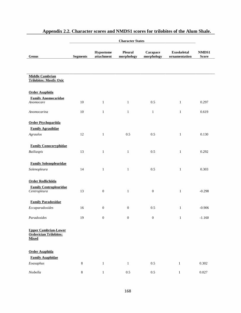
168
Appendix 2.2. Character scores and NMDS1 scores for trilobites of the Alum Shale.
Character States
Genus Segments
Hypostome
attachment
Pleural
morphology
Carapace
morphology
Exoskeletal
ornamentation
NMDS1
Score
Middle Cambrian
Trilobites: Mostly Oxic
Order Asaphida
Family Anomocaridae
Anomocare 10 1 1 0.5 1 0.297
Anomocarina 10 1 1 1 1 0.619
Order Ptychopariida
Family Agraulidae
Agraulos 12 1 0.5 0.5 1 0.130
Family Conocoryphidae
Bailiaspis 13 1 1 0.5 1 0.292
Family Solenopleuridae
Solenopleura 14 1 1 0.5 1 0.303
Order Redlichiida
Family Centropleuridae
Centropleura 13 0 1 0 1 -0.298
Family Paradoxidae
Eccaparadoxides 16 0 0 0.5 1 -0.906
Paradoxides 19 0 0 0 1 -1.160
Upper Cambrian-Lower
Ordovician Trilobites:
Mixed
Order Asaphida
Family Asaphidae
Eoasaphus 8 1 1 0.5 1 0.302
Niobella 8 1 0.5 0.5 1 0.027

169
Family Ceratopygidae
Proceratopyge 10 1 1 0.5 1 0.297
Family Idahoiidae
Maladioidella 10 1 0 0.5 1 -0.227
Order Ptychopariida
Family Elviniidae
Irvingella 12 1 1 0.5 1 0.295
Family Olenidae
Acerocare 12 1 1 0.5 1 0.295
Ctenopyge 8 1 0 0 1 -0.490
Leptoplastides 11 1 0.5 0.5 1 0.025
Leptoplastus 10 1 0.5 0.5 1 0.022
Olenus 14 1 0.5 0.5 1 0.021
Parabolina 13 1 1 0 1 0.085
Parabolinella 14 1 1 1 1 0.610
Parabolinites 14 1 0.5 0.5 1 0.021
Peltura 12 1 0.5 0 1 -0.266
Protopeltura 8 1 1 0.5 1 0.302
Sphaerophthalmus 10 1 0 0 1 -0.475
Note: Middle Cambrian trilobites represent a mostly oxic assemblage while lower Cambrian to early Ordovician trilobites represent a mixed (more dysoxic) assemblage. See Table 2.2 for description of character states. NMDS1 score reflects the
overall similarity of the morphology to an olenimorphic body plan, with high scores being more olenimorphic.
Data adapted from published descriptions by Berg-Madsen (1985), Clarkson and Taylor (1995), and Terfelt et al. (2011)

170
Appendix 2.3. NMDS scores of all trilobites from both datasets, before and after
removal of segmentation from the NMDS model, with the net shift along each axis.
Genus Scores with
segmentation
Scores without
segmentation
Shift in
NMDS1
Shift in
NMDS2
NMDS1 NMDS2 NMDS1 NMDS2
Alum Shale
dataset
Acerocare 0.295 -0.092 0.216 -0.157 -0.079 -0.065
Agraulos 0.013 0.144 0.071 0.247 0.058 0.103
Anomocare 0.297 -0.086 0.216 -0.157 -0.081 -0.071
Anomocarina 0.619 0.060 0.695 -0.045 0.076 -0.105
Bailiaspis 0.292 -0.097 0.216 -0.157 -0.077 -0.060
Centropleura -0.298 -0.806 -0.329 -0.836 -0.031 -0.030
Ctenopyge -0.490 0.426 -0.441 0.359 0.049 -0.068
Eccaparadoxides -0.905 -0.256 -1.032 -0.181 -0.126 0.075
Eoasaphus 0.302 -0.088 0.216 -0.157 -0.087 -0.069
Irvingella 0.295 -0.092 0.216 -0.157 -0.079 -0.065
Leptoplastides 0.023 0.152 0.071 0.247 0.049 0.095
Leptoplastus 0.022 0.156 0.071 0.247 0.050 0.091
Maladioidella -0.227 0.457 -0.414 0.376 -0.187 -0.080
Niobella 0.027 0.170 0.071 0.247 0.044 0.077
Olenus 0.021 0.147 0.071 0.247 0.050 0.100
Parabolina 0.085 -0.390 0.120 -0.247 0.035 0.143
Parabolinella 0.610 0.054 0.695 -0.045 0.085 -0.099
Parabolinites 0.021 0.147 0.071 0.247 0.050 0.100
Paradoxides -1.160 -0.185 -1.013 -0.261 0.147 -0.077
Peltura -0.267 0.027 0.006 0.292 0.273 0.266
Proceratopyge 0.297 -0.086 0.216 -0.157 -0.081 -0.071
Protopeltura 0.302 -0.088 0.216 -0.157 -0.087 -0.069
Solenopleura 0.303 -0.106 0.216 -0.157 -0.087 -0.051
Sphaerophthalmus -0.475 0.430 -0.441 0.359 0.034 -0.072
Early-to-middle
Cambrian dataset
Acadolenus 0.534 0.152 0.589 0.139 0.055 -0.013
Acadoparadoxides -0.526 0.068 -0.508 0.099 0.018 0.031
Agraulos 0.356 -0.128 0.352 -0.149 -0.004 -0.021
Alokistocare 0.381 -0.141 0.352 -0.149 -0.029 -0.008
Alokistocarella 0.789 0.046 0.732 0.093 -0.057 0.047
Altiocculus 0.780 0.231 0.589 0.139 -0.191 -0.092
Asaphiscus 0.749 0.072 0.732 0.093 -0.017 0.021
Bailiella 0.557 -0.236 0.530 -0.229 -0.027 0.007
Bathyuriscus 0.340 -0.115 0.352 -0.149 0.012 -0.034

171
Bolaspidella -0.071 0.615 -0.069 0.625 0.002 0.010
Brachyaspidion 0.202 -0.197 0.333 -0.174 0.131 0.023
Bristolia -1.225 -0.093 -1.253 -0.150 -0.028 -0.057
Bythicheilus 0.365 -0.126 0.352 -0.149 -0.013 -0.023
Chancia 0.594 0.151 0.589 0.139 -0.004 -0.012
Conocoryphe 0.364 -0.123 0.352 -0.149 -0.012 -0.026
Ctenocephalus 0.540 -0.248 0.530 -0.229 -0.010 0.019
Dorypyge -1.044 -0.591 -1.100 -0.501 -0.056 0.091
Eccaparadoxides 0.193 -0.455 0.263 -0.441 0.070 0.013
Ehmaniella 0.359 -0.130 0.352 -0.149 -0.007 -0.019
Ellipsocephalus 0.531 0.133 0.589 0.139 0.058 0.006
Elrathia 0.535 0.136 0.589 0.139 0.054 0.003
Eoredlichia -0.234 0.766 -0.242 0.762 -0.008 -0.004
Estaingia -0.227 0.409 -0.283 0.330 -0.056 -0.078
Germaropyge 0.749 0.043 0.732 0.093 -0.017 0.050
Glossopleura -1.046 -0.540 -1.100 -0.501 -0.054 0.039
Hanburia -0.093 0.660 -0.069 0.625 0.024 -0.035
Hemirhodon 0.034 0.791 -0.003 0.714 -0.038 -0.077
Holyoakia -0.459 0.374 -0.430 0.450 0.029 0.075
Hydrocephalus -0.273 0.295 -0.295 0.313 -0.022 0.018
Hypermecaspis 0.777 0.049 0.732 0.093 -0.045 0.044
Jenkinsonia 0.036 -0.556 0.084 -0.508 0.049 0.048
Jincella 0.536 0.144 0.589 0.139 0.053 -0.005
Kingaspis 0.181 -0.192 0.333 -0.174 0.152 0.018
Kootenia -1.043 -0.310 -1.067 -0.296 -0.024 0.014
Kuanyangia -0.833 -0.526 -0.875 -0.467 -0.042 0.059
Litavkaspis 0.378 -0.135 0.352 -0.149 -0.026 -0.014
Lobocephalina 0.189 -0.447 0.263 -0.441 0.074 0.005
Marjumia 0.386 -0.601 0.327 -0.581 -0.059 0.020
Megapharanaspis -0.701 0.197 -0.691 0.213 0.010 0.016
Mesonacis -1.210 -0.119 -1.253 -0.150 -0.043 -0.031
Modocia 0.384 -0.595 0.327 -0.581 -0.058 0.014
Ogygopsis -0.086 0.633 -0.069 0.625 0.017 -0.007
Olenellus -1.201 -0.123 -1.253 -0.150 -0.052 -0.027
Olenoides -1.225 -0.093 -1.253 -0.150 -0.028 -0.057
Ornamentaspis 0.532 -0.243 0.530 -0.229 -0.002 0.015
Orria -0.086 0.633 -0.069 0.625 0.017 -0.007
Oryctocara -0.085 0.630 -0.069 0.625 0.016 -0.004
Oryctocephalites -0.547 -0.112 -0.534 -0.008 0.013 0.104
Oryctocephalus -0.307 0.306 -0.295 0.313 0.012 0.007
Palaeolenus 0.747 0.060 0.732 0.093 -0.015 0.033
Parabailiella -0.148 -0.775 -0.184 -0.777 -0.036 -0.001
Paradoxides 0.114 -0.615 0.084 -0.508 -0.029 0.107

172
Parkaspis -0.720 0.217 -0.691 0.213 0.029 -0.004
Peachella -0.963 0.691 -1.017 0.686 -0.054 -0.006
Ptychoparella 0.557 0.131 0.589 0.139 0.033 0.008
Ptychoparia 0.535 0.136 0.589 0.139 0.054 0.003
Redlichia -0.450 0.364 -0.430 0.450 0.021 0.086
Sao 0.007 -0.978 0.033 -0.981 0.026 -0.003
Skreiaspis 0.535 0.136 0.589 0.139 0.054 0.003
Spencella 0.359 -0.130 0.352 -0.149 -0.007 -0.019
Spencia 0.356 -0.128 0.352 -0.149 -0.004 -0.021
Syspacephalus 0.583 0.377 0.559 0.289 -0.024 -0.088
Thoracocare -0.279 0.519 -0.283 0.330 -0.004 -0.189
Utaspis 0.189 -0.447 0.263 -0.441 0.074 0.005
Wutingaspis -0.218 0.393 -0.283 0.330 -0.066 -0.062
Yunnanocephalus 0.202 -0.197 0.333 -0.174 0.131 0.023
Zacanthoides -1.235 -0.110 -1.253 -0.150 -0.018 -0.040
Appendix 2.4. R code for NMDS analysis.
#Prepare a dataset for MDS analysis
trilo.mds <- trilo1
#Start MDS and generate scree plot of stress as dimensionality increases
library(vegan)
trilo.mds.1 <- metaMDS(trilo.mds, distance="euclidean", k=1, autotransform=FALSE, noshare=FALSE)
trilo.mds.2 <- metaMDS(trilo.mds, distance="euclidean", k=2, autotransform=FALSE, noshare=FALSE)
trilo.mds.3 <- metaMDS(trilo.mds, distance="euclidean", k=3, autotransform=FALSE, noshare=FALSE)
trilo.mds.4 <- metaMDS(trilo.mds, distance="euclidean", k=4, autotransform=FALSE, noshare=FALSE)
dev.new()
barplot(c(trilo.mds.1$stress, trilo.mds.2$stress, trilo.mds.3$stress, trilo.mds.4$stress), xlab="Dimensions",
ylab="Stress", names.arg=1:4, las=1)
#Plot the MDS analyses
dev.new()
trilo.mds.2$points[,1] <- trilo.mds.2$points[,1]*-1
t.points <- trilo.mds.2$points
#Segment score
plot(trilo.mds.2, type="t", display=c("species"), las=1, xlim=c(min(t.points[1:length(segments)])-.25,
max(t.points[1:length(segments)])+.5))
points(t.points[seg.score==2,], pch=2, col="blue", cex=1)
points(t.points[seg.score==0,], pch=17, col="orange", cex=1)
points(t.points[seg.score==1,], pch=9, col="violet", cex=1)
points(mean(t.points[seg.score==2,1]), mean(t.points[seg.score==2,2]), pch=4, lwd=2, cex=1.5)
points(mean(t.points[seg.score==0,1]), mean(t.points[seg.score==0,2]), pch=4, lwd=2, cex=1.5)
points(mean(t.points[seg.score==1,1]), mean(t.points[seg.score==1,2]), pch=4, lwd=2, cex=1.5)
legend(.45, -0.8, c("High # Segments","Med # Segments","Low # Segments", "Centroids"),
pch=c(2,9,17,4), col=c("blue","violet","orange","black"))
#Carapace morphology
dev.new()

173
plot(trilo.mds.2, type="t", display=c("species"), las=1, xlim=c(min(t.points[1:length(segments)])-.25,
max(t.points[1:length(segments)])+.5))
points(t.points[carap.morph==1,], pch=2, col="blue", cex=1)
points(t.points[carap.morph==0,], pch=17, col="orange", cex=1)
points(t.points[carap.morph==.5,], pch=9, col="violet", cex=1)
points (mean(t.points[carap.morph==1,1]), mean(t.points[carap.morph==1,2]), pch=4, lwd=2, cex=1.5)
points (mean(t.points[carap.morph==0,1]), mean(t.points[carap.morph==0,2]), pch=4, lwd=2, cex=1.5)
points (mean(t.points[carap.morph==.5,1]), mean(t.points[carap.morph==.5,2]), pch=4, lwd=2)
legend(.34, -.8, c("Flat Carapace","Arched Carapace","Highly Arched Carap.", "Centroids"),
pch=c(2,9,17,4), col=c("blue","violet","orange","black"))
#Pleural morphology
dev.new()
plot(trilo.mds.2, type="t", display=c("species"), las=1, xlim=c(min(t.points[1:length(segments)])-.25,
max(t.points[1:length(segments)])+.5))
points(t.points[pleur.morph==1,], pch=2, col="blue", cex=1)
points(t.points[pleur.morph==0,], pch=17, col="orange", cex=1)
points(t.points[pleur.morph==.5,], pch=9, col="violet", cex=1)
points (mean(t.points[pleur.morph==1,1]), mean(t.points[pleur.morph==1,2]), pch=4, lwd=2, cex=1.5)
points (mean(t.points[pleur.morph==0,1]), mean(t.points[pleur.morph==0,2]), pch=4, lwd=2, cex=1.5)
points (mean(t.points[pleur.morph==.5,1]), mean(t.points[pleur.morph==.5,2]), pch=4, lwd=2)
legend(.45, -.8, c("Flat Pleurae","Arched Pleurae","Arched and Spiny", "Centroids"), pch=c(2,9,17,4),
col=c("blue","violet","orange","black"))
#Hypostome attachment
dev.new()
plot(trilo.mds.2, type="t", display=c("species"), las=1, xlim=c(min(t.points[1:length(segments)])-.25,
max(t.points[1:length(segments)])+.5))
points(t.points[hypost.att==1,], pch=2, col="blue", cex=1)
points(t.points[hypost.att==0,], pch=17, col="orange", cex=1)
points (mean(t.points[hypost.att==1,1]), mean(t.points[hypost.att==1,2]), pch=4, lwd=2, cex=1.5)
points (mean(t.points[hypost.att==0,1]), mean(t.points[hypost.att==0,2]), pch=4, lwd=2, cex=1.5)
legend(.25, -.8, c("Non-Attached Hypostome", "Attached Hypostome", "Centroids"), pch=c(2,17,4),
col=c("blue","orange","black"))
#Ornamentation
dev.new()
plot(trilo.mds.2, type="t", display=c("species"), las=1, xlim=c(min(t.points[1:length(segments)])-.25,
max(t.points[1:length(segments)])+.5))
points(t.points[exosk.ornam==1,], pch=2, col="blue", cex=1)
points(t.points[exosk.ornam==0,], pch=17, col="orange", cex=1)
points (mean(t.points[exosk.ornam==1,1]), mean(t.points[exosk.ornam==1,2]), pch=4, lwd=2, cex=1.5)
points (mean(t.points[exosk.ornam==0,1]), mean(t.points[exosk.ornam==0,2]), pch=4, lwd=2, cex=1.5)
legend(.45, -.8, c("Not Ornamented","Ornamented", "Centroids"), pch=c(2,17,4),
col=c("blue","orange","black"))
dev.new()
plot(trilo.mds.2, type="n", display=c("species"), las=1, xlim=c(min(t.points[1:length(segments)])-.25,
max(t.points[1:length(segments)])+.5))
points(t.points[,1], t.points[,2], col="black", pch=16, cex=.5)
points(t.points[row.names(t.points)=="Elrathia",1], t.points[row.names(t.points)=="Elrathia",2], pch=17,
cex=1.5)
points(t.points[row.names(t.points)=="Hypermecaspis",1],
t.points[row.names(t.points)=="Hypermecaspis",2], pch=2, cex=1.5)
points(t.points[row.names(t.points)=="Olenellus",1], t.points[row.names(t.points)=="Olenellus",2], pch=9,
cex=1.5)
points(.76, .4727, pch=1, cex=1.5)
points(-.4651, .3558, pch=3, cex=1.5)
points(-.4727, .3646, pch=4, cex=1.5)

174
legend(.55, -.5, c("Hypermecaspis","Elrathia","Olenellus","Triarthrus","Phacops","Greenops"),
pch=c(2,17,9,1,3,4))
#Order
dev.new()
plot(trilo.mds.2, type="n", display=c("species"), las=1, xlim=c(min(t.points[1:length(segments)])-.25,
max(t.points[1:length(segments)])+.5))
points(t.points[trilo1$Order=="Corynexochida",1], t.points[trilo1$Order=="Corynexochida",2], pch=4,
col="orange", cex=1)
points(t.points[trilo1$Order=="Ptychopariida",1], t.points[trilo1$Order=="Ptychopariida",2], pch=2,
col="blue", cex=1)
points(t.points[trilo1$Order=="Redlichiida",1], t.points[trilo1$Order=="Redlichiida",2], pch=9,
col="violet", cex=1)
legend(.45, -.8, c("Ptychopariida","Corynexochida","Redlichiida"), pch=c(2,4,9),
col=c("blue","orange","violet"))
#Environment, Ptychs
dev.new()
plot(trilo.mds.2, type="n", display=c("species"), las=1, xlim=c(min(t.points[1:length(segments)])-.25,
max(t.points[1:length(segments)])+.5))
points(t.points[trilo1$Order=="Ptychopariida"&trilo1$LOC=="1",1],
t.points[trilo1$Order=="Ptychopariida"&trilo1$LOC=="1",2], pch=9, col="blue", cex=1)
points (mean(t.points[trilo1$Order=="Ptychopariida"&trilo1$LOC==1,1]),
mean(t.points[trilo1$Order=="Ptychopariida"&trilo1$LOC==1,2]), pch=4, lwd=2, cex=1.5)
points(t.points[trilo1$Order=="Ptychopariida"&trilo1$LOC==0,1],
t.points[trilo1$Order=="Ptychopariida"&trilo1$LOC==0,2], pch=2, col="orange", cex=1)
points (mean(t.points[trilo1$Order=="Ptychopariida"&trilo1$LOC==0,1]),
mean(t.points[trilo1$Order=="Ptychopariida"&trilo1$LOC==0,2]), pch=4, lwd=2, cex=1.5)
legend(.45, -.8, c("Mixed","Mostly Oxic","Centroids"), pch=c(2,9,4), col=c("orange","blue","black"))
#Environment, Reds
dev.new()
plot(trilo.mds.2, type="n", display=c("species"), las=1, xlim=c(min(t.points[1:length(segments)])-.25,
max(t.points[1:length(segments)])+.5))
points(t.points[trilo1$Order=="Corynexochida"&trilo1$LOC=="1",1],
t.points[trilo1$Order=="Corynexochida"&trilo1$LOC=="1",2], pch=9, col="blue", cex=1)
points (mean(t.points[trilo1$Order=="Corynexochida"&trilo1$LOC==1,1]),
mean(t.points[trilo1$Order=="Corynexochida"&trilo1$LOC==1,2]), pch=4, lwd=2, cex=1.5)
points(t.points[trilo1$Order=="Corynexochida"&trilo1$LOC==0,1],
t.points[trilo1$Order=="Corynexochida"&trilo1$LOC==0,2], pch=2, col="orange", cex=1)
points (mean(t.points[trilo1$Order=="Corynexochida"&trilo1$LOC==0,1]),
mean(t.points[trilo1$Order=="Corynexochida"&trilo1$LOC==0,2]), pch=4, lwd=2, cex=1.5)
legend(.45, -.8, c("Mixed","Mostly Oxic","Centroids"), pch=c(2,9,4), col=c("orange","blue","black"))
#Environment, Corys
dev.new()
plot(trilo.mds.2, type="n", display=c("species"), las=1, xlim=c(min(t.points[1:length(segments)])-.25,
max(t.points[1:length(segments)])+.5))
points(t.points[trilo1$Order=="Redlichiida"&trilo1$LOC=="1",1],
t.points[trilo1$Order=="Redlichiida"&trilo1$LOC=="1",2], pch=9, col="blue", cex=1)
points (mean(t.points[trilo1$Order=="Redlichiida"&trilo1$LOC==1,1]),
mean(t.points[trilo1$Order=="Redlichiida"&trilo1$LOC==1,2]), pch=4, lwd=2, cex=1.5)
points(t.points[trilo1$Order=="Redlichiida"&trilo1$LOC==0,1],
t.points[trilo1$Order=="Redlichiida"&trilo1$LOC==0,2], pch=2, col="orange", cex=1)
points (mean(t.points[trilo1$Order=="Redlichiida"&trilo1$LOC==0,1]),
mean(t.points[trilo1$Order=="Redlichiida"&trilo1$LOC==0,2]), pch=4, lwd=2, cex=1.5)
legend(.45, -.8, c("Mixed","Mostly Oxic","Centroids"), pch=c(2,9,4), col=c("orange","blue","black"))
#Get MDS loadings
trilo.mds.2$species
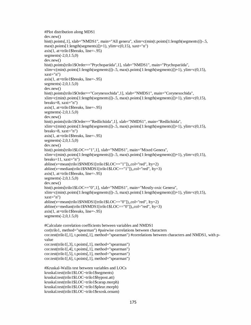
175
#Plot distribution along MDS1
dev.new()
hist(t.points[,1], xlab="NMDS1", main="All genera", xlim=c(min(t.points[1:length(segments)])-.5,
max(t.points[1:length(segments)])+1), ylim=c(0,15), xaxt="n")
axis(1, at=trilo1$breaks, line=-.95)
segments(-2,0,1.5,0)
dev.new()
hist(t.points[trilo1$Order=="Ptychopariida",1], xlab="NMDS1", main="Ptychopariida",
xlim=c(min(t.points[1:length(segments)])-.5, max(t.points[1:length(segments)])+1), ylim=c(0,15),
xaxt="n")
axis(1, at=trilo1$breaks, line=-.95)
segments(-2,0,1.5,0)
dev.new()
hist(t.points[trilo1$Order=="Corynexochida",1], xlab="NMDS1", main="Corynexochida",
xlim=c(min(t.points[1:length(segments)])-.5, max(t.points[1:length(segments)])+1), ylim=c(0,15),
breaks=8, xaxt="n")
axis(1, at=trilo1$breaks, line=-.95)
segments(-2,0,1.5,0)
dev.new()
hist(t.points[trilo1$Order=="Redlichiida",1], xlab="NMDS1", main="Redlichiida",
xlim=c(min(t.points[1:length(segments)])-.5, max(t.points[1:length(segments)])+1), ylim=c(0,15),
breaks=8, xaxt="n")
axis(1, at=trilo1$breaks, line=-.95)
segments(-2,0,1.5,0)
dev.new()
hist(t.points[trilo1$LOC=="1",1], xlab="NMDS1", main="Mixed Genera",
xlim=c(min(t.points[1:length(segments)])-.5, max(t.points[1:length(segments)])+1), ylim=c(0,15),
breaks=11, xaxt="n")
abline(v=mean(trilo1$NMDS1[trilo1$LOC=="1"]),,col="red", lty=2)
abline(v=median(trilo1$NMDS1[trilo1$LOC=="1"]),,col="red", lty=3)
axis(1, at=trilo1$breaks, line=-.95)
segments(-2,0,1.5,0)
dev.new()
hist(t.points[trilo1$LOC=="0",1], xlab="NMDS1", main="Mostly-oxic Genera",
xlim=c(min(t.points[1:length(segments)])-.5, max(t.points[1:length(segments)])+1), ylim=c(0,15),
xaxt="n")
abline(v=mean(trilo1$NMDS1[trilo1$LOC=="0"]),,col="red", lty=2)
abline(v=median(trilo1$NMDS1[trilo1$LOC=="0"]),,col="red", lty=3)
axis(1, at=trilo1$breaks, line=-.95)
segments(-2,0,1.5,0)
#Calculate correlation coefficients between variables and NMDS1
cor(trilo1, method="spearman") #pairwise correlations between characters
cor.test(trilo1[,1], t.points[,1], method="spearman") #correlations between characters and NMDS1, with p-
value
cor.test(trilo1[,3], t.points[,1], method="spearman")
cor.test(trilo1[,4], t.points[,1], method="spearman")
cor.test(trilo1[,5], t.points[,1], method="spearman")
cor.test(trilo1[,6], t.points[,1], method="spearman")
#Kruskal-Wallis test between variables and LOCs
kruskal.test(trilo1$LOC~trilo1$segments)
kruskal.test(trilo1$LOC~trilo1$hypost.att)
kruskal.test(trilo1$LOC~trilo1$carap.morph)
kruskal.test(trilo1$LOC~trilo1$pleur.morph)
kruskal.test(trilo1$LOC~trilo1$exosk.ornam)

176
#Welch two-sample t-test between taxonomic orders
t.test(trilo1$NMDS1[trilo1$Order=="Corynexochida"], trilo1$NMDS1[trilo1$Order=="Redlichiida"])
t.test(trilo1$NMDS1[trilo1$Order=="Ptychopariida"], trilo1$NMDS1[trilo1$Order=="Redlichiida"])
t.test(trilo1$NMDS1[trilo1$Order=="Corynexochida"], trilo1$NMDS1[trilo1$Order=="Ptychopariida"])
#Welch two-sample t-test between oxic/dysoxic
t.test(trilo1$NMDS1[trilo1$LOC=="0"], trilo1$NMDS[trilo1$LOC=="1"])
#Welch two-sample t-test between oxic ptychs/dysoxic ptychs
t.test(trilo1$NMDS1[trilo1$LOC=="0"&trilo1$Order=="Ptychopariida"],
trilo1$NMDS[trilo1$LOC=="1"&trilo1$Order=="Ptychopariida"])
#One-sample T-tests
t.test(trilo1$NMDS1[trilo1$Order=="Ptychopariida"])
t.test(trilo1$NMDS1[trilo1$Order=="Ptychopariida"&trilo1$NMDS>0.4908])
#Determine number of clusters
dev.new()
wss <- (nrow(t.points)-1)*sum(apply(t.points,2,var))
for (i in 2:15) wss[i] <- sum(kmeans(t.points,
centers=i)$withinss)
plot(1:15, wss, type="b", xlab="Number of Clusters",
ylab="Within groups sum of squares")
#run K-means analysis
km <- kmeans(t.points, centers=6, nstart=20, iter.max=100)
#plot K-means results
dev.new()
plot(trilo.mds.2, type="n", display=c("species"), las=1, xlim=c(min(t.points[1:length(segments)])-.25,
max(t.points[1:length(segments)])+.5))
points(t.points[km$cluster==1,1], t.points[km$cluster==1,2], pch=4, col="orange", cex=1)
points(t.points[km$cluster==2,1], t.points[km$cluster==2,2], pch=5, col="red", cex=1)
points(t.points[km$cluster==3,1], t.points[km$cluster==3,2], pch=6, col="purple", cex=1)
points(t.points[km$cluster==4,1], t.points[km$cluster==4,2], pch=3, col="blue", cex=1)
points(t.points[km$cluster==5,1], t.points[km$cluster==5,2], pch=8, col="green", cex=1)
points(t.points[km$cluster==6,1], t.points[km$cluster==6,2], pch=9, col="brown", cex=1)
#Logistic Regression of Environment Type as a function of NMDS1 scores
lr <- glm(trilo1$LOC~trilo1$NMDS1, family="binomial")
summary(lr)
layout(matrix(1:4,2,2))
plot(lr)

177
Appendix 3.1. Supplementary methods for biomarker analyses.
Trilobites were quarried commercially from the middle Cambrian Wheeler Shale by
professional collectors (West Desert Collectors and Terra Trilobites, Delta UT) from rock
depths up to 5 meters representing rock with little, if any, weathering. Two specimens of
Elrathia and 16 Peronopsis with robust and complete exoskeletons were used (Fig. 3.1).
The 16 Peronopsis were combined into two sets of eight for analysis, to yield a
comparable sample mass to the Elrathia and ensure sufficient material for analysis.
Because compounds from anthropogenic polymers are particularly pervasive, to
minimize plastic contamination, two additional Elrathia kingii and five Peronopsis, both
with associated sediment, were collected and protected from contact with any type of
plastics during extraction, shipping, and handling. The five protected Peronopsis were
combined for analysis, but did not yield any compounds above the detection limit, despite
repeated tests on the sample material, and thus these samples could not be interpreted.
Total carbon for sediments was determined by powdering sediment samples
associated with both trilobite species in a Spex 8000 ball mill to produce approximately
20 ml of powdered sediment. 100 mg of these powders were weighed into a crucible
boat and fired on an Eltra furnace to 1350°C under a pure oxygen atmosphere. The
resultant carbon dioxide was measured by infrared absorption on an Eltra CS500
determinator to yield the total weight percent carbon in the sample. Total inorganic
carbon was then determined by weighing another 100 mg of the same sample powder into
a 250 ml flask and mixing with 10 ml of ethanol, then connecting the flask to an Eltra
CS500 determinator, adding 10 ml of 20% HCl and heating to 50°C, and measuring the
resultant carbon dioxide as above. Total organic carbon was determined by subtracting
178
the inorganic carbon from the total carbon for each sample, and averaging values by
species. Carbon and inorganic carbon analysis was performed at the Lyons Lab at UC
Riverside.
Sediment and exoskeletal samples were prepared for multibiomarker analysis by GC-
MS, yielding a profile of individual biomarkers present in each sample, following a
multibiomarker method established by Medeiros and Simoneit (Medeiros and Simoneit,
2007, 2008a, 2008b) and Simoneit et al. (2014). This method allows for a simultaneous
characterization of the different chemical classes spanning a wide range of polarities,
without a need to isolate certain chemical classes before analysis. Protected samples
were rinsed with Milli-Q water upon arrival, and after drying, they were gently rinsed
with dichloromethane followed by methanol and left to dry again at room temperature.
All samples were powdered in a solvent pre-cleaned ball mill and then weighed in a pre-
combusted (450°C for 5 h) beaker. Samples were then sonicated twice for 15 min in a 30
mL mixture of dichloromethane:methanol (2:1, v/v). The extract aliquots were combined
and filtered using a Gelman Swinney filtration unit containing an annealed pre-
combusted glass fiber filter (42.5 mm, Whatman) for the removal of insoluble particles.
The filtrate was first concentrated in a RapidVap (solvent evaporation system) to about
1.5 mL, then further to 500 μL using a stream of high-purity nitrogen. Aliquots of the
total extracts were evaporated completely using a stream of filtered nitrogen gas, and then
converted to their trimethylsilyl derivatives using BSTFA containing 1% TMCS and
pyridine for 3 h at 70°C. Immediately before GC-MS analysis, derivatized extracts were
evaporated to dryness using nitrogen gas and redissolved in hexane for injection.
179
Aliquots of 1 μL of silylated total extracts were analyzed within 24 hours using a HP
6890 gas chromatograph interfaced with a HP 5975 mass selective detector (GC-MS). A
DB5-MS capillary column (30 m x 0.25 mm I.D. and film thickness of 0.25 m) was
used with helium as the carrier gas at a constant flow rate of 1.3 mL min-1
. The injector
and MS source temperatures were maintained at 280°C and 230°C, respectively. The
column temperature program consisted of injection at 65°C and hold for 2 min,
temperature increase of 6°C min-1
to 300°C, followed by an isothermal hold at 300°C for
15 min. The MS was operated in the electron impact mode with an ionization energy of
70 eV. The scan range was set from 50 to 650 Da and the samples were analyzed in
splitless mode.
Data were acquired and processed with the HP-Chemstation software. Individual
compounds were identified by comparison of mass spectra with literature and library
data, comparison of mass spectra and GC retention times with those of authentic
standards and/or interpretation of mass spectrometric fragmentation patterns.
Compounds were quantified using the total ion current (TIC) peak area, and converted to
compound mass using calibration curves of external standards: n-eicosene for n-alkanes,
isoprenoids, UCM, and phthalates; n-hexadecanoic acid for n-alkanoic acids, n-alkanols
and glyceride derivatives; lupeol for diterpenoids, sterols and lignin derivatives; glucose
for monosaccharides; sucrose for disaccharides. A procedural blank was run in sequence
to samples, presenting no significant background interferences.

180
Appendix 3.2. Concentrations (10-9
g g-1
) of biomarkers and other chemical compounds present in middle Cambrian
Wheeler Shale trilobites and sediment samples. Samples include exoskeletal material (exos.) from Elrathia kingii (Elr)
and Peronopsis (Per), and sediments (sed.) associated with both trilobites and from the broader Wheeler Shale (WS).
Protected samples were guarded against contact with plastics during collection and transport.
Unprotected samples Protected samples
Elr Elr Per Per WS WS Elr Elr Elr Elr Per
exos. exos. exos. exos. sed. sed. exos. exos. sed. sed. sed.
Chemical Class
Individual
Compound
n-Alkanes
Heptadecane 0.0 0.0 0.0 0.0 13.1 0.0 0.0 0.0 0.0 0.0 0.0
Octadecane 0.0 0.0 0.0 0.0 41.7 6.7 0.0 14.1 0.0 0.0 1.7
Nonadecane 0.0 0.0 0.0 0.0 37.0 12.2 0.0 0.0 0.0 0.0 0.0
Eicosane 0.0 0.0 0.0 0.0 0.0 11.4 0.0 0.0 0.0 0.0 4.3
Tetracosane 62.6 33.4 96.0 334.1 0.0 0.0 0.0 0.0 0.0 0.0 0.0
Pentacosane 49.6 37.3 142.3 543.4 0.0 12.1 0.0 0.0 0.0 0.0 0.0
Hexacosane 82.8 44.4 147.1 817.6 0.0 0.0 0.0 0.0 0.0 0.0 0.0
Heptacosane 61.8 29.9 91.4 729.4 0.0 0.0 0.0 0.0 0.0 0.0 0.0
Octacosane 38.4 22.8 71.8 599.2 0.0 0.0 0.0 0.0 0.0 0.0 0.0
Nonacosane 35.2 15.0 0.0 453.2 0.0 0.0 0.0 0.0 0.0 0.0 0.0
Triacontane 19.9 10.4 0.0 324.5 0.0 0.0 0.0 0.0 0.0 0.0 0.0
Total 350.2 193.1 548.6 3801.4 91.9 42.3 0.0 14.1 0.0 0.0 6.0
CPIa 0.7 0.7 0.7 0.8 - - - - - - -
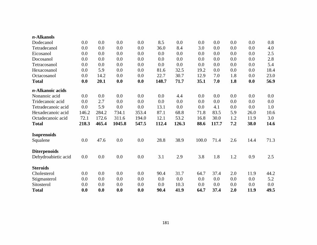
181
n-Alkanols
Dodecanol 0.0 0.0 0.0 0.0 8.5 0.0 0.0 0.0 0.0 0.0 0.8
Tetradecanol 0.0 0.0 0.0 0.0 36.0 8.4 3.0 0.0 0.0 0.0 4.0
Eicosanol 0.0 0.0 0.0 0.0 0.0 0.0 0.0 0.0 0.0 0.0 2.5
Docosanol 0.0 0.0 0.0 0.0 0.0 0.0 0.0 0.0 0.0 0.0 2.8
Tetracosanol 0.0 0.0 0.0 0.0 0.0 0.0 0.0 0.0 0.0 0.0 5.4
Hexacosanol 0.0 5.9 0.0 0.0 81.6 32.5 19.2 0.0 0.0 0.0 18.4
Octacosanol 0.0 14.2 0.0 0.0 22.7 30.7 12.9 7.0 1.8 0.0 23.0
Total 0.0 20.1 0.0 0.0 148.7 71.7 35.1 7.0 1.8 0.0 56.9
n-Alkanoic acids
Nonanoic acid 0.0 0.0 0.0 0.0 0.0 4.4 0.0 0.0 0.0 0.0 0.0
Tridecanoic acid 0.0 2.7 0.0 0.0 0.0 0.0 0.0 0.0 0.0 0.0 0.0
Tetradecanoic acid 0.0 5.9 0.0 0.0 13.1 0.0 0.0 4.1 0.0 0.0 1.0
Hexadecanoic acid 146.2 284.2 734.1 353.4 87.1 68.8 71.8 83.5 5.9 26.0 10.6
Octadecanoic acid 72.1 172.6 311.6 194.0 12.1 53.2 16.8 30.0 1.2 11.9 3.0
Total 218.3 465.4 1045.8 547.5 112.4 126.3 88.6 117.7 7.2 38.0 14.6
Isoprenoids
Squalene 0.0 47.6 0.0 0.0 28.8 38.9 100.0 71.4 2.6 14.4 71.3
Diterpenoids
Dehydroabietic acid 0.0 0.0 0.0 0.0 3.1 2.9 3.8 1.8 1.2 0.9 2.5
Steroids
Cholesterol 0.0 0.0 0.0 0.0 90.4 31.7 64.7 37.4 2.0 11.9 44.2
Stigmasterol 0.0 0.0 0.0 0.0 0.0 0.0 0.0 0.0 0.0 0.0 5.2
Sitosterol 0.0 0.0 0.0 0.0 0.0 10.3 0.0 0.0 0.0 0.0 0.0
Total
0.0 0.0 0.0 0.0 90.4 41.9 64.7 37.4 2.0 11.9 49.5

182
Lignin derivatives
Vanillin 0.0 0.0 0.0 0.0 2.7 0.0 0.0 0.0 0.0 0.0 3.9
3-Methoxy-
Benzaldehyde 0.0 0.0 0.0 0.0 0.0 0.0 0.0 0.0 0.0 0.0 8.2
Total 0.0 0.0 0.0 0.0 2.7 0.0 0.0 0.0 0.0 0.0 12.1
Saccharides
α- + β-Glucose 0.0 0.0 0.0 0.0 222.0 244.0 401.5 146.9 2315.1 5513.1 2.7
α- + β-Fructose 0.0 0.0 0.0 0.0 0.0 0.0 0.0 0.0 220.1 900.4 0.0
Dulcitol 0.0 0.0 0.0 0.0 0.0 0.0 0.0 0.0 40.3 209.2 0.0
myo-Inositol 0.0 0.0 0.0 0.0 35.2
13.8
15.0
10.5
0.0 0.0 0.0 0.0 0.0
scillo-Inositol 0.0 0.0 0.0 0.0 4.8 0.0 0.0 0.0 0.0
Levoglucosan 0.0 0.0 90.2 7.0 3.1 1.7 2.3 1.3 14.9 16.6 1.2
Sucrose 0.0 0.0 0.0 0.0 233.1 146.5 0.0 28.0 4.8 40.1 2.1
Mycose 0.0 0.0 0.0 0.0 0.0 10.8 0.0 0.0 0.0 0.0 0.0
Total 0.0 0.0 90.2 7.0 507.2 428.4 408.5 176.3 2595.1 6679.4 5.9
Glyceride
derivatives
Glycerol 0.0 0.0 0.0 0.0 0.0 8.7 0.0 0.0 0.0 0.0 0.0
1-O-Hexadecanoyl
glycerol 0.0 0.0 0.0 0.0 30.5 4.8 19.5 12.4 0.0 0.0 6.5
1-O-Octadecanoyl
glycerol 0.0 0.0 0.0 0.0 2.4 2.6 0.0 0.0 0.0 0.0 1.1
Total 0.0 0.0 0.0 0.0 32.9 16.2 19.5 12.4 0.0 0.0 7.6
Amides
Benzamide 0.0 0.0 0.0 0.0 10.5 0.0 0.0 0.0 0.0 0.0 0.0
m-Toluamide 0.0 0.0 0.0 0.0 0.0 8.5 0.0 0.0 0.0 0.0 0.0
Total 0.0 0.0 0.0 0.0 10.5 8.5 0.0 0.0 0.0 0.0 0.0
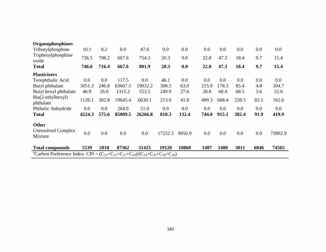
183
Organophosphines
Tributylphosphine 10.1 8.2 0.0 47.6 0.0 0.0 0.0 0.0 0.0 0.0 0.0
Triphenylphosphine
oxide 736.5 708.2 667.6 754.3 20.3 0.0 22.8 47.3 18.4 9.7 15.4
Total 746.6 716.4 667.6 801.9 20.3 0.0 22.8 47.3 18.4 9.7 15.4
Plasticizers
Terephthalic Acid 0.0 0.0 117.5 0.0 46.1 0.0 0.0 0.0 0.0 0.0 0.0
Butyl phthalate 3051.3 246.8 63667.5 19032.2 308.3 63.0 215.9 178.3 85.4 4.8 204.7
Butyl hexyl phthalate 46.9 26.0 1315.2 553.5 249.9 27.6 28.8 68.4 68.5 3.6 52.6
Bis(2-ethylhexyl)
phthalate 1126.1 302.8 19645.4 6630.1 213.9 41.8 499.3 668.4 228.5 83.5 162.6
Phthalic Anhydride 0.0 0.0 264.0 51.0 0.0 0.0 0.0 0.0 0.0 0.0 0.0
Total 4224.3 575.6 85009.5 26266.8 818.3 132.4 744.0 915.1 382.4 91.9 419.9
Other
Unresolved Complex
Mixture 0.0 0.0 0.0 0.0 17252.5 9950.9 0.0 0.0 0.0 0.0 73902.9
Total compounds 5539 2018 87362 31425 19120 10860 1487 1400 3011 6846 74565 aCarbon Preference Index. CPI = (C23+C25+C27+C29)/(C24+C26+C28+C30)
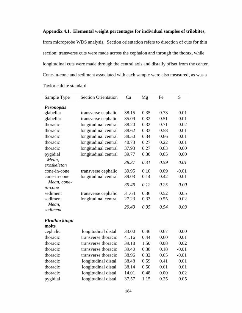
184
Appendix 4.1. Elemental weight percentages for individual samples of trilobites,
from microprobe WDS analysis. Section orientation refers to direction of cuts for thin
section: transverse cuts were made across the cephalon and through the thorax, while
longitudinal cuts were made through the central axis and distally offset from the center.
Cone-in-cone and sediment associated with each sample were also measured, as was a
Taylor calcite standard.
Sample Type Section Orientation Ca Mg Fe S
Peronopsis
glabellar transverse cephalic 38.15 0.35 0.73 0.01
glabellar transverse cephalic 35.09 0.32 0.51 0.01
thoracic longitudinal central 38.20 0.32 0.71 0.02
thoracic longitudinal central 38.62 0.33 0.58 0.01
thoracic longitudinal central 38.50 0.34 0.66 0.01
thoracic longitudinal central 40.73 0.27 0.22 0.01
thoracic longitudinal central 37.93 0.27 0.63 0.00
pygidial longitudinal central 39.77 0.30 0.65 0.00
Mean,
exoskeleton 38.37 0.31 0.59 0.01
cone-in-cone transverse cephalic 39.95 0.10 0.09 -0.01
cone-in-cone longitudinal central 39.03 0.14 0.42 0.01
Mean, cone-
in-cone 39.49 0.12 0.25 0.00
sediment transverse cephalic 31.64 0.36 0.52 0.05
sediment longitudinal central 27.23 0.33 0.55 0.02
Mean,
sediment 29.43 0.35 0.54 0.03
Elrathia kingii
molts
cephalic longitudinal distal 33.00 0.46 0.67 0.00
thoracic transverse thoracic 41.16 0.44 0.60 0.01
thoracic transverse thoracic 39.18 1.50 0.08 0.02
thoracic transverse thoracic 39.40 0.38 0.18 -0.01
thoracic transverse thoracic 38.96 0.32 0.65 -0.01
thoracic longitudinal distal 38.48 0.59 0.41 0.01
thoracic longitudinal distal 38.14 0.50 0.61 0.01
thoracic longitudinal distal 14.01 0.48 0.00 0.02
pygidial longitudinal distal 37.57 1.15 0.25 0.05
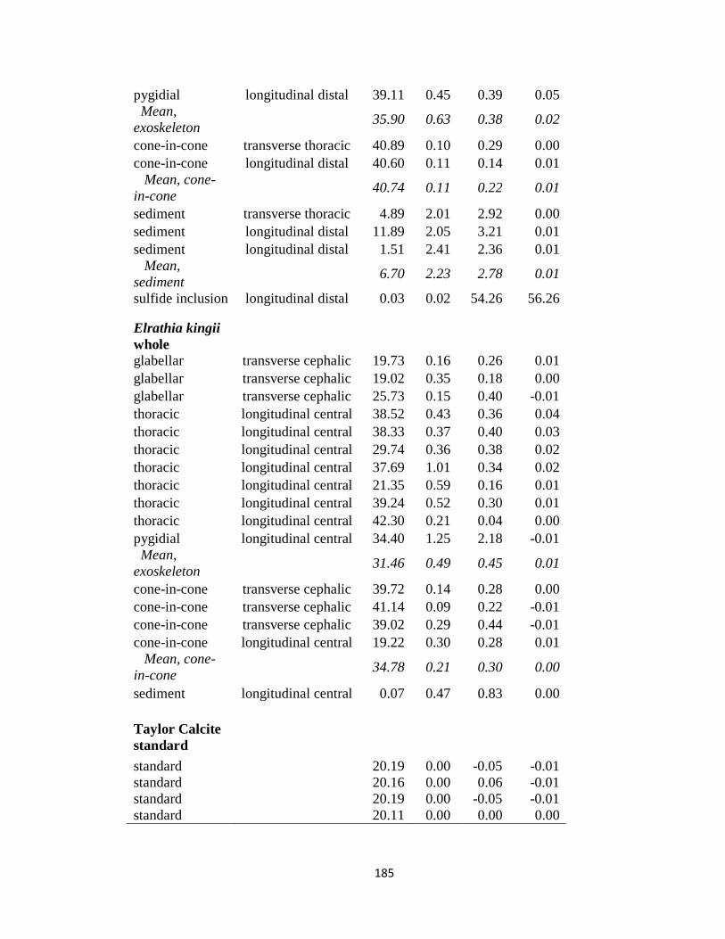
185
pygidial longitudinal distal 39.11 0.45 0.39 0.05
Mean,
exoskeleton 35.90 0.63 0.38 0.02
cone-in-cone transverse thoracic 40.89 0.10 0.29 0.00
cone-in-cone longitudinal distal 40.60 0.11 0.14 0.01
Mean, cone-
in-cone 40.74 0.11 0.22 0.01
sediment transverse thoracic 4.89 2.01 2.92 0.00
sediment longitudinal distal 11.89 2.05 3.21 0.01
sediment longitudinal distal 1.51 2.41 2.36 0.01
Mean,
sediment 6.70 2.23 2.78 0.01
sulfide inclusion longitudinal distal 0.03 0.02 54.26 56.26
Elrathia kingii
whole
glabellar transverse cephalic 19.73 0.16 0.26 0.01
glabellar transverse cephalic 19.02 0.35 0.18 0.00
glabellar transverse cephalic 25.73 0.15 0.40 -0.01
thoracic longitudinal central 38.52 0.43 0.36 0.04
thoracic longitudinal central 38.33 0.37 0.40 0.03
thoracic longitudinal central 29.74 0.36 0.38 0.02
thoracic longitudinal central 37.69 1.01 0.34 0.02
thoracic longitudinal central 21.35 0.59 0.16 0.01
thoracic longitudinal central 39.24 0.52 0.30 0.01
thoracic longitudinal central 42.30 0.21 0.04 0.00
pygidial longitudinal central 34.40 1.25 2.18 -0.01
Mean,
exoskeleton 31.46 0.49 0.45 0.01
cone-in-cone transverse cephalic 39.72 0.14 0.28 0.00
cone-in-cone transverse cephalic 41.14 0.09 0.22 -0.01
cone-in-cone transverse cephalic 39.02 0.29 0.44 -0.01
cone-in-cone longitudinal central 19.22 0.30 0.28 0.01
Mean, cone-
in-cone 34.78 0.21 0.30 0.00
sediment longitudinal central 0.07 0.47 0.83 0.00
Taylor Calcite
standard
standard 20.19 0.00 -0.05 -0.01
standard 20.16 0.00 0.06 -0.01
standard 20.19 0.00 -0.05 -0.01
standard 20.11 0.00 0.00 0.00

186
Appendix 5.1. Total carbon and sulfur data, from infrared absorption spectrometry.
Alpha Resources AR 4007 ore standard was run before and after specimens, and blank
crucibles were also run.
Sample Total C (wt. %) Total S (wt. %)
Standard 7.17 3.83
Standard 7.18 4.31
Standard 7.44 4.42
Standard 7.22 4.65
Standard 7.18 3.42
Standard 7.20 3.35
1 3.16 0.11
2 5.84 0.04
3 3.05 0.06
4 3.50 0.03
5 2.89 0.12
6 3.21 0.00
7 2.92 0.12
8 3.14 0.00
9 4.30 0.11
10 2.93 0.09
11 4.64 0.00
12 2.63 0.00
13 6.73 0.00
14 3.45 0.06
15 3.06 0.12
16 4.41 0.04
17 3.13 0.00
18 3.39 0.08
19 5.20 0.00
20 4.75 0.00
21 3.16 0.02
22 5.12 0.00
23 5.25 0.00
24 3.98 0.00
25 3.87 0.00
Blank 0.05 0.02
Blank 0.02 0.00
Standard 7.34 3.25
Standard 7.32 3.35
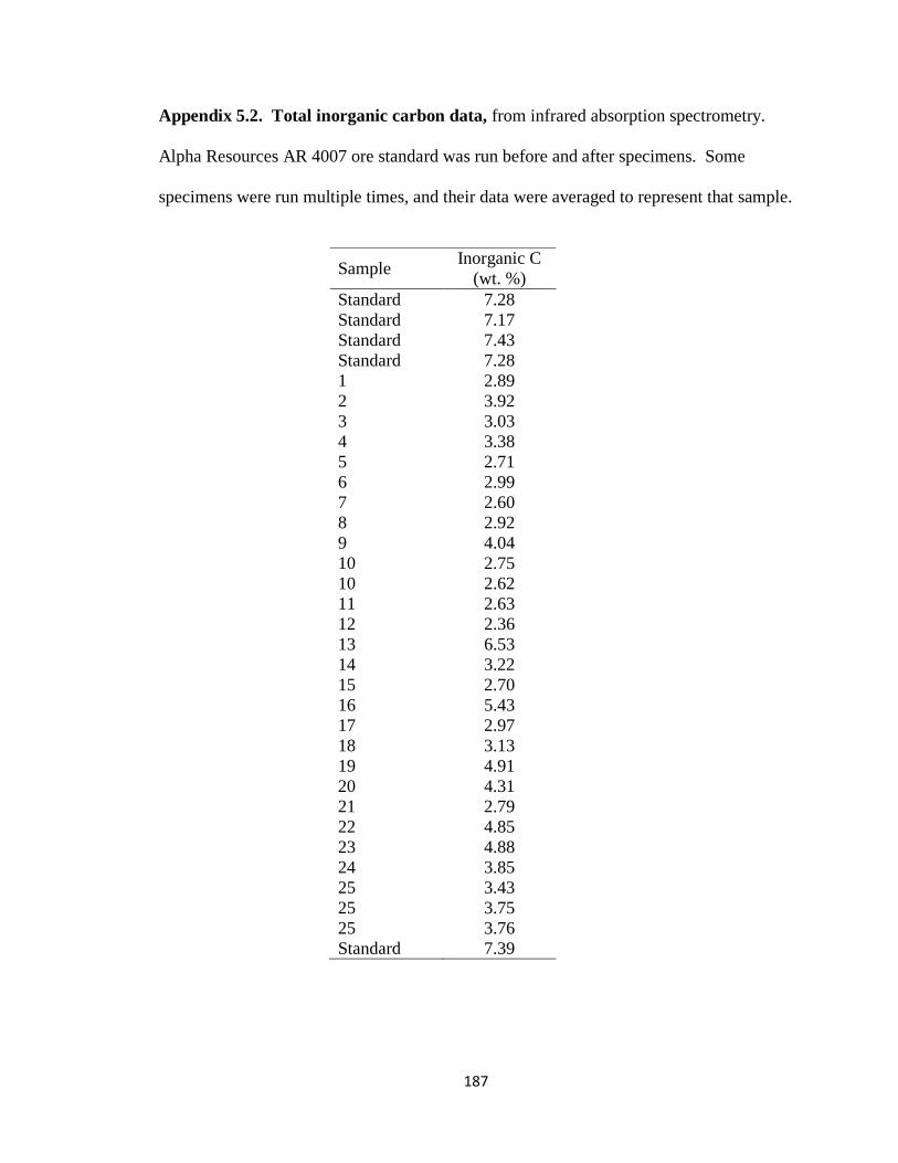
187
Appendix 5.2. Total inorganic carbon data, from infrared absorption spectrometry.
Alpha Resources AR 4007 ore standard was run before and after specimens. Some
specimens were run multiple times, and their data were averaged to represent that sample.
Sample Inorganic C
(wt. %)
Standard 7.28
Standard 7.17
Standard 7.43
Standard 7.28
1 2.89
2 3.92
3 3.03
4 3.38
5 2.71
6 2.99
7 2.60
8 2.92
9 4.04
10 2.75
10 2.62
11 2.63
12 2.36
13 6.53
14 3.22
15 2.70
16 5.43
17 2.97
18 3.13
19 4.91
20 4.31
21 2.79
22 4.85
23 4.88
24 3.85
25 3.43
25 3.75
25 3.76
Standard 7.39

188
Appendix 5.3. Weight percent Spy from Cr reduction analysis.
Sample Wt. % Spyr
1 0.14
2 0.09
3 0.12
4 0.06
5 0.16
6 0.03
7 0.19
8 0.19
9 0.13
10 0.25
11 0.06
12 0.12
13 0.09
14 0.15
15 0.25
16 0.07
17 0.02
18 0.24
19 0.15
20 0.19
21 0.17
22 0.17
23 0.15
24 0.04
25 0.02

189
Appendix 5.4. Mg, Al, Ca, Mn and Fe data from sequential Fe extraction. 25
samples and a blank were analyzed by ICP-MS after extracting metals from sediments in
acetate, dithionite, and oxalate solutions, representing reactive Fe from carbonates,
simple oxides, and multivalent oxides, respectively.
Raw ICP-MS Data (counts) Mg Al Ca Mn Fe
Sample 24
Mg 27
Al 43
Ca 55
Mn 56
Fe wt. % wt. % wt. % ppm wt. %
Acetate
1 1.33 0.042 8.79 25.79 0.71 1.22 0.04 8.08 23.70 0.65
2 0.87 0.012 18.36 33.11 0.59 0.86 0.01 18.34 33.07 0.59
3 0.90 0.022 7.28 20.06 0.52 0.89 0.02 7.22 19.88 0.51
4 1.24 0.016 8.95 25.25 0.69 1.30 0.02 9.39 26.48 0.72
5 0.74 0.005 5.47 16.03 0.44 0.81 0.01 5.98 17.52 0.48
6 1.07 0.008 7.29 22.19 0.58 1.10 0.01 7.51 22.85 0.60
7 1.06 0.010 5.98 19.44 0.57 1.10 0.01 6.19 20.12 0.59
8 0.99 0.013 7.61 20.52 0.58 1.02 0.01 7.83 21.12 0.60
9 1.29 0.014 11.36 30.05 0.74 1.24 0.01 10.88 28.79 0.71
10 0.75 0.013 7.72 16.54 0.43 0.72 0.01 7.37 15.81 0.41
11 0.98 0.017 16.57 34.43 0.57 1.00 0.02 16.94 35.19 0.59
12 1.13 0.024 6.79 19.31 0.56 1.12 0.02 6.76 19.23 0.56
13 0.70 0.007 19.00 32.33 0.46 0.71 0.01 19.44 33.09 0.47
14 1.19 0.015 8.31 24.77 0.68 1.13 0.01 7.88 23.48 0.64
15 0.96 0.021 5.96 19.57 0.59 0.95 0.02 5.93 19.47 0.59
16 0.77 0.007 11.22 25.10 0.46 0.70 0.01 10.15 22.71 0.41
17 1.13 0.024 7.70 22.07 0.64 1.12 0.02 7.67 21.97 0.64
18 1.34 0.020 8.81 25.87 0.71 1.28 0.02 8.41 24.69 0.68
19 0.87 0.017 13.71 26.44 0.54 0.87 0.02 13.75 26.52 0.54
20 1.02 0.012 14.81 31.35 0.56 0.96 0.01 13.88 29.39 0.52
21 0.60 0.017 7.26 14.82 0.35 0.62 0.02 7.40 15.10 0.35
22 1.07 0.042 16.58 32.37 0.67 1.05 0.04 16.34 31.91 0.66
23 0.90 0.029 16.26 32.43 0.56 0.82 0.03 14.93 29.77 0.52
24 0.77 0.012 12.20 41.78 0.25 0.77 0.01 12.18 41.71 0.25
25 0.72 0.018 10.51 39.38 0.24 0.69 0.02 10.16 38.05 0.23
Blank -0.01 -0.027 -0.14 -2.89 -0.12 0.00 0.00 -0.01 -0.28 -0.01
Dithionite
1 0.05 0.011 0.41 3.58 0.05 0.05 0.01 0.38 3.26 0.04
2 0.04 0.008 0.49 3.18 0.02 0.04 0.01 0.47 3.02 0.02
3 0.04 0.008 0.22 2.88 0.02 0.04 0.01 0.21 2.82 0.02
4 0.05 0.013 0.36 3.41 0.18 0.05 0.01 0.36 3.46 0.18
5 0.04 0.011 0.31 3.06 0.04 0.04 0.01 0.32 3.17 0.05
6 0.04 0.012 0.25 3.13 0.16 0.04 0.01 0.25 3.10 0.16
7 0.04 0.009 0.24 2.91 0.07 0.04 0.01 0.24 2.90 0.07
8 0.05 0.010 0.32 3.15 0.03 0.05 0.01 0.32 3.12 0.03
9 0.05 0.009 0.33 3.33 0.03 0.05 0.01 0.32 3.26 0.03

190
10 0.04 0.009 0.29 3.04 0.04 0.04 0.01 0.26 2.76 0.03
11 0.04 0.019 0.34 3.34 0.27 0.04 0.02 0.34 3.31 0.27
12 0.04 0.015 0.25 3.04 0.17 0.04 0.01 0.25 3.04 0.17
13 0.04 0.007 0.45 3.21 0.03 0.04 0.01 0.45 3.20 0.03
14 0.05 0.010 0.29 3.02 0.04 0.05 0.01 0.29 3.02 0.04
15 0.05 0.009 0.28 2.98 0.02 0.05 0.01 0.28 3.02 0.02
16 0.04 0.011 0.37 3.28 0.14 0.04 0.01 0.34 3.04 0.13
17 0.04 0.012 0.22 2.94 0.17 0.04 0.01 0.23 3.03 0.17
18 0.05 0.010 0.30 3.09 0.02 0.05 0.01 0.28 2.86 0.02
19 0.05 0.009 0.43 3.35 0.03 0.05 0.01 0.42 3.31 0.03
20 0.06 0.011 0.52 3.54 0.03 0.06 0.01 0.54 3.63 0.03
21 0.04 0.011 0.39 3.36 0.05 0.05 0.01 0.40 3.38 0.05
22 0.04 0.010 0.40 3.37 0.03 0.05 0.01 0.41 3.44 0.03
23 0.05 0.010 0.53 3.52 0.05 0.04 0.01 0.50 3.28 0.05
24 0.04 0.026 0.27 3.53 0.32 0.04 0.02 0.26 3.43 0.31
25 0.04 0.028 0.26 3.48 0.36 0.04 0.03 0.24 3.24 0.34
Blank 0.02 0.004 0.12 2.39 -0.01 0.00 0.00 0.01 0.24 0.00
Oxalate
1 0.02 0.018 0.03 0.19 0.05 0.02 0.02 0.03 0.17 0.05
2 0.04 0.007 0.04 0.83 0.06 0.04 0.01 0.04 0.81 0.06
3 0.02 0.015 0.03 0.12 0.05 0.02 0.01 0.03 0.12 0.05
4 0.02 0.037 0.04 0.13 0.05 0.02 0.04 0.04 0.13 0.06
5 0.02 0.012 0.03 0.07 0.04 0.02 0.01 0.03 0.07 0.04
6 0.01 0.010 0.03 -0.01 0.04 0.01 0.01 0.03 -0.01 0.04
7 0.02 0.014 0.03 0.05 0.04 0.02 0.01 0.03 0.05 0.04
8 0.03 0.060 0.04 0.18 0.05 0.03 0.06 0.04 0.18 0.05
9 0.04 0.014 0.04 0.49 0.06 0.03 0.01 0.03 0.47 0.05
10 0.02 0.016 0.03 0.10 0.05 0.02 0.02 0.03 0.10 0.04
11 0.02 0.021 0.04 0.07 0.06 0.02 0.02 0.04 0.07 0.06
12 0.02 0.044 0.04 0.02 0.05 0.02 0.05 0.04 0.03 0.05
13 0.04 0.014 0.03 0.61 0.07 0.04 0.01 0.04 0.64 0.07
14 0.03 0.038 0.04 0.18 0.05 0.03 0.04 0.04 0.18 0.05
15 0.03 0.033 0.03 0.14 0.05 0.03 0.03 0.04 0.14 0.05
16 0.03 0.017 0.03 0.22 0.05 0.03 0.02 0.03 0.21 0.05
17 0.02 0.033 0.04 0.09 0.05 0.02 0.03 0.04 0.10 0.06
18 0.03 0.019 0.04 0.22 0.05 0.03 0.02 0.04 0.22 0.05
19 0.04 0.029 0.04 0.32 0.06 0.04 0.03 0.04 0.34 0.06
20 0.04 0.022 0.07 0.51 0.06 0.04 0.02 0.07 0.50 0.06
21 0.03 0.060 0.05 0.27 0.06 0.03 0.06 0.05 0.28 0.06
22 0.03 0.037 0.04 0.44 0.06 0.04 0.04 0.04 0.46 0.07
23 0.03 0.014 0.03 0.42 0.06 0.03 0.01 0.03 0.42 0.06
24 0.02 0.043 0.04 0.09 0.10 0.02 0.04 0.04 0.09 0.10
25 0.01 0.022 0.04 0.04 0.07 0.01 0.02 0.04 0.04 0.08
Blank 0.00 -0.008 0.03 -0.07 0.03 0.00 0.00 0.00 -0.01 0.00

191
Appendix 5.5. Metal concentrations from total metal digest. Some samples were analyzed twice. All units are in ppm.
Sample 23
Na 24
Mg 27
Al 31
P 39
K 44
Ca 47
Ti 56
Fe 51
V 52
Cr 55
Mn 59
Co
1 3553.2 29698.7 91302.3 285.5 21669.0 20140.5 3588.4 33295.8 97.87 84.78 270.95 16.67
2 2440.0 18958.5 41009.6 101.6 9328.9 35996.1 2165.4 26122.0 95.79 84.68 335.66 25.99
3 3105.9 18301.2 61700.4 145.9 17684.7 12701.8 2167.4 22397.6 102.82 89.93 310.39 13.21
4 3312.8 21755.6 68629.6 369.6 21393.9 18194.2 2643.3 24364.3 73.27 61.60 323.94 11.48
5 2995.9 26188.3 83914.5 215.4 19055.3 18301.2 3582.8 33362.0 53.40 45.81 443.16 8.37
6 2773.7 24191.0 75711.6 146.3 17124.3 19758.4 3496.2 31614.4 93.29 83.15 305.50 13.50
6 3132.4 25225.3 69444.8 167.3 18871.9 16966.3 2982.6 28119.3 94.77 82.95 335.56 13.90
7 2546.0 16940.9 53344.6 153.0 16191.9 9502.2 2124.1 18372.5 70.92 62.36 392.26 11.46
8 2871.5 21261.4 70565.7 61.3 17134.5 16304.0 2823.6 27951.1 85.65 75.92 247.57 13.23
9 2779.3 25123.4 59203.8 170.5 13720.8 25495.3 2872.6 31838.6 70.21 60.78 476.94 10.41
10 3589.4 24496.7 83812.6 237.0 21113.7 17455.4 3022.9 27237.8 82.49 78.72 315.07 12.46
11 3080.9 23559.3 69241.0 197.0 14026.5 32042.4 2919.9 30483.3 95.53 81.98 339.73 15.10
12 3195.6 24420.3 86818.7 288.9 19896.0 15514.3 3331.6 30651.5 81.83 73.01 253.22 19.60
13 2752.8 17710.2 38482.5 7.7 7831.0 44265.3 1816.4 25444.4 83.71 69.50 259.18 21.16
14 2926.1 20823.2 56248.7 119.0 17159.9 15733.3 2488.9 23192.4 93.60 80.14 310.08 17.23
15 2635.1 21200.3 63076.0 257.0 15840.3 16028.9 3146.7 31492.2 65.73 55.94 320.22 9.95
16 3105.9 18474.4 59917.1 20.0 14444.3 26020.1 2511.8 24410.1 68.43 58.69 453.81 10.36
17 3675.0 29010.9 89264.3 254.3 19473.1 18097.4 3223.1 29296.2 84.27 74.44 285.22 6.89
18 3597.1 27339.7 79227.2 139.9 17659.2 17577.7 2829.3 28501.4 54.47 45.76 345.39 8.27
19 2096.1 14755.1 32592.7 8.8 9058.9 20894.6 1522.9 17480.9 80.45 69.04 276.81 17.63
20 3352.0 20680.6 63432.7 132.2 14281.3 30524.1 2670.8 27793.2 82.34 72.40 247.16 18.37
21 2833.3 19254.0 68222.0 84.6 16956.1 15921.9 2495.5 23467.5 76.22 65.98 301.32 8.52
22 3173.2 23452.3 57216.8 126.5 12177.0 31996.6 2320.8 28134.6 78.46 68.94 272.79 10.98
23 3673.5 23854.8 67661.5 135.2 12890.3 39012.4 2939.3 31268.0 71.58 61.04 344.47 10.72
24 2769.6 24140.1 68833.4 224.2 15820.0 25429.1 2635.1 33637.1 61.04 51.20 334.23 8.71
24 2271.3 20884.4 61598.5 75.6 13945.0 23151.7 2452.7 29000.7 59.46 53.09 414.53 9.80
25 2585.2 25373.1 71380.9 204.1 15534.6 29601.9 3104.4 36113.3 63.38 52.27 327.15 10.37
Std 2036.5 8824.5 58898.1 290.5 22438.4 1917.2 3489.1 60579.5 145.00 54.26 281.04 40.64
Std 2081.8 7515.1 56299.7 322.6 20925.1 1681.9 3366.3 59305.7 150.35 55.28 288.38 40.54
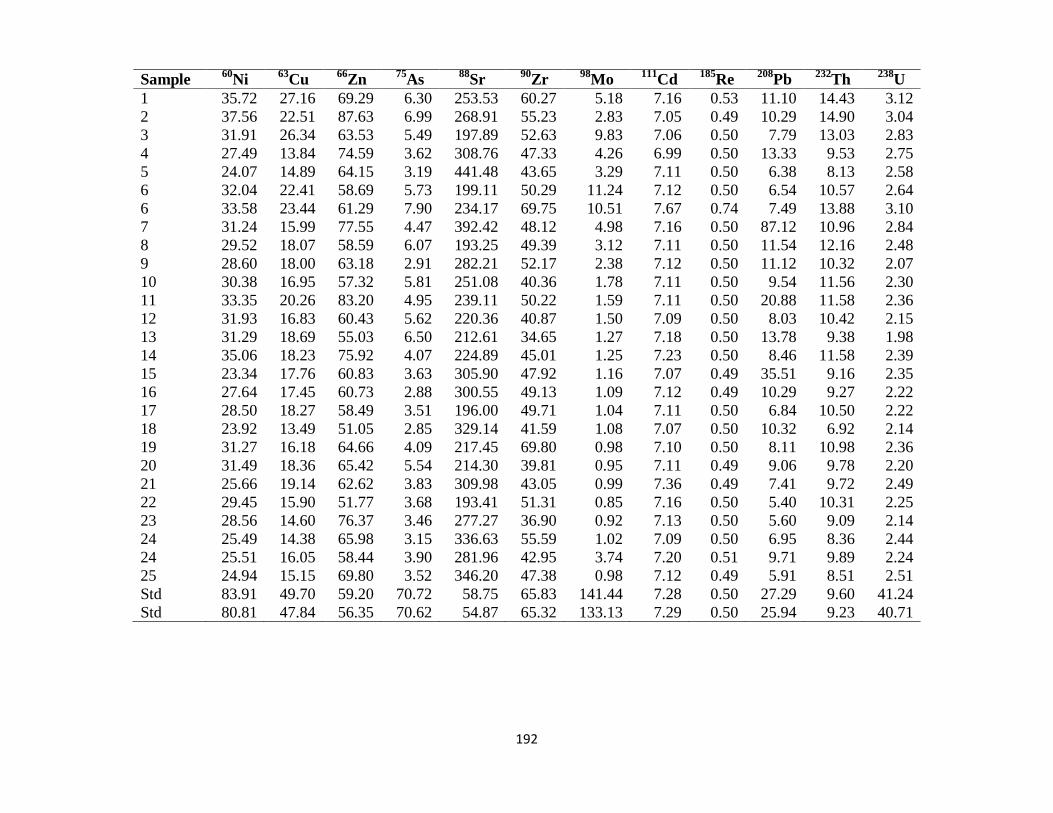
192
Sample 60
Ni 63
Cu 66
Zn 75
As 88
Sr 90
Zr 98
Mo 111
Cd 185
Re 208
Pb 232
Th 238
U
1 35.72 27.16 69.29 6.30 253.53 60.27 5.18 7.16 0.53 11.10 14.43 3.12
2 37.56 22.51 87.63 6.99 268.91 55.23 2.83 7.05 0.49 10.29 14.90 3.04
3 31.91 26.34 63.53 5.49 197.89 52.63 9.83 7.06 0.50 7.79 13.03 2.83
4 27.49 13.84 74.59 3.62 308.76 47.33 4.26 6.99 0.50 13.33 9.53 2.75
5 24.07 14.89 64.15 3.19 441.48 43.65 3.29 7.11 0.50 6.38 8.13 2.58
6 32.04 22.41 58.69 5.73 199.11 50.29 11.24 7.12 0.50 6.54 10.57 2.64
6 33.58 23.44 61.29 7.90 234.17 69.75 10.51 7.67 0.74 7.49 13.88 3.10
7 31.24 15.99 77.55 4.47 392.42 48.12 4.98 7.16 0.50 87.12 10.96 2.84
8 29.52 18.07 58.59 6.07 193.25 49.39 3.12 7.11 0.50 11.54 12.16 2.48
9 28.60 18.00 63.18 2.91 282.21 52.17 2.38 7.12 0.50 11.12 10.32 2.07
10 30.38 16.95 57.32 5.81 251.08 40.36 1.78 7.11 0.50 9.54 11.56 2.30
11 33.35 20.26 83.20 4.95 239.11 50.22 1.59 7.11 0.50 20.88 11.58 2.36
12 31.93 16.83 60.43 5.62 220.36 40.87 1.50 7.09 0.50 8.03 10.42 2.15
13 31.29 18.69 55.03 6.50 212.61 34.65 1.27 7.18 0.50 13.78 9.38 1.98
14 35.06 18.23 75.92 4.07 224.89 45.01 1.25 7.23 0.50 8.46 11.58 2.39
15 23.34 17.76 60.83 3.63 305.90 47.92 1.16 7.07 0.49 35.51 9.16 2.35
16 27.64 17.45 60.73 2.88 300.55 49.13 1.09 7.12 0.49 10.29 9.27 2.22
17 28.50 18.27 58.49 3.51 196.00 49.71 1.04 7.11 0.50 6.84 10.50 2.22
18 23.92 13.49 51.05 2.85 329.14 41.59 1.08 7.07 0.50 10.32 6.92 2.14
19 31.27 16.18 64.66 4.09 217.45 69.80 0.98 7.10 0.50 8.11 10.98 2.36
20 31.49 18.36 65.42 5.54 214.30 39.81 0.95 7.11 0.49 9.06 9.78 2.20
21 25.66 19.14 62.62 3.83 309.98 43.05 0.99 7.36 0.49 7.41 9.72 2.49
22 29.45 15.90 51.77 3.68 193.41 51.31 0.85 7.16 0.50 5.40 10.31 2.25
23 28.56 14.60 76.37 3.46 277.27 36.90 0.92 7.13 0.50 5.60 9.09 2.14
24 25.49 14.38 65.98 3.15 336.63 55.59 1.02 7.09 0.50 6.95 8.36 2.44
24 25.51 16.05 58.44 3.90 281.96 42.95 3.74 7.20 0.51 9.71 9.89 2.24
25 24.94 15.15 69.80 3.52 346.20 47.38 0.98 7.12 0.49 5.91 8.51 2.51
Std 83.91 49.70 59.20 70.72 58.75 65.83 141.44 7.28 0.50 27.29 9.60 41.24
Std 80.81 47.84 56.35 70.62 54.87 65.32 133.13 7.29 0.50 25.94 9.23 40.71