RESEARCH ARTICLE10.1002/2015MS000578

Exploring historical and future urban climate in the EarthSystem Modeling framework: 1. Model development andevaluationDan Li1,2, Sergey Malyshev3, and Elena Shevliakova4

1Program of Atmospheric and Oceanic Sciences, Princeton University, Princeton, New Jersey, USA, 2Department of Earthand Environment, Boston University, Boston, Massachusetts, USA, 3Department of Ecology and Evolutionary Biology,Princeton University, Princeton, New Jersey, USA, 4Geophysical Fluid Dynamics Laboratory, Princeton, New Jersey, USA

Abstract A number of recent studies investigated impacts of Land-Use and Land-Cover Changes (LULCC)on climate with global Earth System Models (ESMs). Yet many ESMs are still missing a representation of themost extreme form of natural landscape modification – urban settlements. Moreover, long-term (i.e., deca-des to century) transitions between build-up and other land cover types due to urbanization and de-urbanization have not been examined in the literature. In this study we evaluate a new urban canopy model(UCM) that characterizes urban physical and biogeochemical processes within the subgrid tiling frameworkof the Geophysical Fluid Dynamics Laboratory (GFDL) land model, LM3. The new model LM3-UCM is basedon the urban canyon concept and simulates exchange of energy, water (liquid and solid), and carbonbetween urban land and the atmosphere. LM3-UCM has several unique features, including explicit treat-ment of vegetation inside the urban canyon and dynamic transition between urban, agricultural andunmanaged tiles. The model is evaluated using observational data sets collected at three urban sites: Mar-seille in France, Basel in Switzerland and Baltimore in the United States. It is found that LM3-UCM satisfacto-rily reproduces canyon air temperature, surface temperatures, radiative fluxes, and turbulent heat fluxes atthe three urban sites. LM3-UCM can capture urban features in a computationally efficient manner and isincorporated into the land component of GFDL ESMs. This new capability will enable improved understand-ing of climate change effects on cities and the impacts of urbanization on climate.

1. Introduction

Land-Use and Land-Cover Changes (LULCC) at local, regional and global scales have been shown to play animportant role in modulating the Earth’s climate, its hydrological and biogeochemical cycles [Findell et al.,2007; Mahmood et al., 2014; Malyshev et al., 2015; Pielke et al., 2011]. Urbanization is an extreme case ofLULCC through which natural landscapes are turned into man-made landscapes. Urbanization alters surfaceaerodynamic, thermodynamic and hydrologic properties, which concomitantly change surface turbulentand energy fluxes and, as a result, surface/near-surface temperatures [Arnfield, 2003; Oke, 1982] as well asprecipitation [Li et al., 2013; Niyogi et al., 2011; Shepherd, 2005]. Buildings and other man-made structures inurban areas also affect the turbulent flow and transport at local, neighborhood and city scales [Bou-Zeidet al., 2009; Wang et al., 2014; Wood et al., 2010; Yu et al., 2013]. Urban areas are important sources of green-house gas emissions as well as anthropogenic heat and aerosol emissions [Grimmond, 2007]. Therefore,quantifying the impacts of urbanization on the climate system at various temporal and spatial scales isimportant for proper representation of land-atmosphere interactions, and has been the subject of activeresearch. Of equal importance is to quantify the impacts of global climate change on urban areas, wheremore than 50% of the world’s population live, and to assess urban mitigation and adaption strategies [Liet al., 2014]. Due to the many unique features of urban areas, it is expected that urban areas will respond ina different way to the global climate change as compared to rural areas [Fischer et al., 2012; Li and Bou-Zeid,2013; Li et al., 2015; McCarthy et al., 2010; Oleson, 2012].

In order to examine the impacts of urbanization on the climate system and the impacts of global climatechange on urban areas, it is important to integrate urban representations into Global Climate Models(GCMs) and Earth System Models (ESMs). There have been continuous efforts toward this goal and

This article is a companion to Li et al.

[2016], doi:10.1002/2015MS000579.

Key Points:� An urban canopy model is developed� The model is suitable for climate and

earth system simulations� The model is validated

Correspondence to:D. Li,lidan@bu.edu

Citation:Li, D., S. Malyshev, and E. Shevliakova(2016), Exploring historical and futureurban climate in the Earth SystemModeling framework: 1. Modeldevelopment and evaluation, J. Adv.Model. Earth Syst., 8, 917–935,doi:10.1002/2015MS000578.

Received 29 OCT 2015

Accepted 11 MAY 2016

Accepted article online 17 MAY 2016

Published online 12 JUN 2016

VC 2016. The Authors.

This is an open access article under

the terms of the Creative Commons

Attribution-NonCommercial-NoDerivs

License, which permits use and

distribution in any medium, provided

the original work is properly cited, the

use is non-commercial and no modifi-

cations or adaptations are made.

LI ET AL. URBAN CLIMATE IN EARTH SYSTEM MODELS 917

Journal of Advances in Modeling Earth Systems

PUBLICATIONS

numerous urban parameterizations, with different levels of complexity, have been proposed. Masson [2006]classified urban parameterizations into three main categories: 1) empirical models that are based on statisticalfitting to observations, 2) modified land surface models (LSMs), originally designed for natural vegetated orbare surfaces and later adapted to represent urban landscapes, and 3) urban canopy models (UCMs). Empiri-cal models that calculate fluxes based on statistical fitting to observations (e.g., assuming that the groundheat flux is a fixed fraction of the net radiation) are usually limited to areas where the observations weretaken. Traditional LSMs, even with modified parameters for urban surfaces (e.g., albedo, emissivity, heatcapacity, thermal conductivity, and roughness length), have been shown to be still inadequate to captureurban fluxes [Grimmond et al., 2010, 2011] and the urban heat island effect [Lee et al., 2011; Zhang et al., 2011].Because UCMs better represent unique urban characteristics (e.g., multiple reflections of radiation amongbuildings), they are receiving more attention even though they usually require a large number of inputs.

The international urban energy balance model comparison project [Grimmond et al., 2010., 2011] systemati-cally compared and evaluated 32 urban parameterization schemes and found that the models generally dowell in simulating radiation exchanges but have strong biases in simulating latent heat fluxes. The morecomplex schemes such as UCMs have more potential for improvements as compared to simpler modelswhose performance is more dependent on parameter calibration. Grimmond et al [2010, 2011] also con-cluded that taking vegetation into account is important, and integrating vegetation into the urban schemebetter captures urban fluxes as compared to treating vegetation separately.

Motivated by the need to better understand both the impacts of global climate change in urban areas andthe feedbacks of urbanization on climate, we develop an UCM in the subgrid tiling framework of GFDL landmodel LM3 [Milly et al., 2014; Shevliakova et al., 2009], which provides surface boundary conditions to theatmosphere. Increasing attention has been given to land models’ capabilities, enabling improved under-standing of the interactions among the hydrological cycle, biophysical and biogeochemical processes, aswell as human activities. This is particularly important when land models are used in ESMs to assess effectsof LULCC [Lawrence et al., 2012]. While urban areas account for a small fraction of global land, the resolutionof ESMs is increasing and the urban sprawl is continuing. Therefore, it is critical to develop a detailed repre-sentation of urban processes for supporting model-based investigations of urban climate, hydrological andbiogeochemical cycles, which is essential for designing sustainability-related strategies and policies forregions with large population densities.

The aim of this paper, which is the first part of a series toward exploring historical and future urban climatewithin GFDL’s Earth System Modeling framework, is to describe a new UCM and to evaluate its performanceusing offline simulations (i.e., land model simulations driven by observational data sets rather than coupledwith a free-running atmospheric model). We also compare our UCM to other UCMs in terms of model struc-ture and performance. The paper is organized as follows: Section 2 describes the model structure. Section 3presents the comparison between simulated results at three urban sites and observations. Section 4 con-cludes the paper.

2. Model Description

2.1. Model RequirementsIn a GCM or an ESM, a land model has to provide bottom boundary conditions for the atmospheric model,with fields such as radiative and turbulent fluxes. Within the GFDL flexible modeling framework [Balaji et al.,2006], LM3 represents each grid-cell’s surface heterogeneity as a collection of tiles [Milly et al., 2014; Shevlia-kova et al., 2009]. Each tile has its own energy and water balances throughout the vegetation-soil columnand its own exchange coefficients with the atmosphere. Contributions of each tile are aggregated at thebottom atmospheric layer so that the atmosphere only feels the area-averaged fluxes [Balaji et al., 2006].The primary goal of our study is to introduce an UCM that handles an urban tile in LM3 (hereafter calledLM3-UCM).

A unique requirement associated with developing an urban parameterization for decadal to century scaleclimate or ESM simulations is that the location and size of the urban area must be dynamic in order to rep-resent transitions from rural land to urban land and vice versa. Allowing urban area to change is also criticalfor assessing the historical and future hydroclimatic impacts of urban expansions, which is one of the over-arching goals of our study. This dynamic feature makes our urban implementation different from most

Journal of Advances in Modeling Earth Systems 10.1002/2015MS000578

LI ET AL. URBAN CLIMATE IN EARTH SYSTEM MODELS 918

other urban parameterizations such as the Community Land Model Urban (CLMU) [Oleson et al., 2008] aswell as the single-layer urban canopy model (SLUCM) [Kusaka et al., 2001] in the Weather Research andForecasting (WRF) model, since in these models urban tiles do not transition from/to other land-cover tilesand these models do not account for, for example, transfers of matter and energy during such transitions.

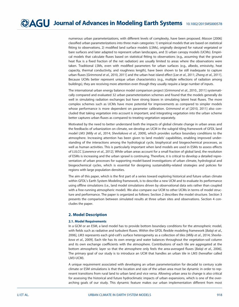
2.2. Model StructureIn light of the above requirements, we design LM3-UCM based on the urban canopy concept (see Figure 1),which is different from many urban parameterizations that do not explicitly consider the canopy structure[Best et al., 2006; Jarvi et al., 2011, 2014]. However, we do not model mass, momentum and energyexchanges at multiple levels within the canopy as compared to multi-layer UCMs [Kondo et al., 2005; Martilliet al., 2002]. The single layer LM3-UCM is composed of two major components: a roof component and acanyon component. These two components do not interact with each other directly; instead, they commu-nicate with the bottom atmospheric layer through which they interact with each other. The canyon compo-nent includes the walls, the impervious surface at the ground, the pervious surface at the ground (i.e., soil),and the vegetation above soil. These are called subcomponents of the urban canyon hereafter. All of thesefour subcomponents communicate with the canopy air in the urban canyon, through which they interactwith each other and also the atmosphere. The area fractions of pervious and impervious ground aredenoted as fP and fIMP (fP 1 fIMP 5 1), respectively. In this paper, we use ‘‘the pervious part of the ground’’ toindicate the combination of vegetation and soil, while ‘‘the impervious part of the ground’’ to indicate theimpervious surface such as pavements. Soil underlies both pervious and impervious ground. Water, heatand carbon are exchanged between soil, vegetation and canopy air. Water and heat are also exchangedbetween impervious ground and canopy air, but the walls and canopy air only exchange sensible heat. Inaddition, heat is exchanged at the interface between soil and the impervious surface. The roof and wallsalso interact with the building interior through conductive heat fluxes but no interactions are allowedbetween buildings and soil.

LM3-UCM is different from the SLUCM in WRF [Kusaka et al., 2001] and the Town Energy Balance (TEB)model [Masson, 2000] in its explicit treatment of vegetation as an integral part of the urban canyon, insteadof considering vegetation outside of the urban canyon as in SLUCM or TEB. However, it is noted that recentimprovements have been made to incorporate vegetation into the urban canyon in the TEB model

Figure 1. A schematic of the LM3 urban canopy model. za is the height of the lowest level in the atmospheric model; H is the averagedheight of buildings; Rf is the roof width and Rd is the canyon width. Troof is the roof surface temperature; Twall is the wall surface tempera-ture; Tbuilding is the temperature of the building interior; Tcanopy is the canopy air temperature within the urban canyon; Tveg is the vegeta-tion temperature; Tsoil is the soil surface temperature; Timp is the impervious surface temperature.

Journal of Advances in Modeling Earth Systems 10.1002/2015MS000578

LI ET AL. URBAN CLIMATE IN EARTH SYSTEM MODELS 919

[Lemonsu et al., 2012] and other single-layer UCMs [Wang et al., 2013]. Our model is conceptually similar tothe CLMU with a few distinct features: first, vegetation is handled by a dynamic vegetation module [Shevlia-kova et al., 2009] here but is parameterized by a simplified bulk scheme in CLMU. In addition, the roof com-ponent of our model communicates with the atmospheric model directly while in CLMU the roofcomponent interacts with the canopy air in the urban canyon, which essentially assumes that the air in theurban canyon and on the roof is well mixed. A recent study using CLMU found that this assumption resultsin higher roof temperature as compared to observations and decoupling the roof from the canyon is impor-tant [Demuzere et al., 2013].

2.3. Physical Parameterizations2.3.1. Shortwave RadiationAt the roof surface, the total downward shortwave radiation flux is a combination of the direct (indicated bythe subscript ‘‘dir’’) solar radiation (S+dir , W m22) and the diffuse (indicated by the subscript ‘‘dif’’) solar radia-tion (S+dif ,W m22) from the atmosphere, so the net shortwave radiation (SR, where the subscript ‘‘R’’ denotesroof) is

SR5 12aR;dir� �

S+dir1 12aR;dif� �

S+dif ; (1)

where aR;dir and aR;dif are the roof albedos for direct and diffuse solar radiation, respectively. Within theurban canyon, radiative exchanges are parameterized following Masson [2000] for direct solar radiation andHarman et al. [2004] for diffuse solar radiation. Below we describe essential features of radiation exchangewithin the urban canyon.

First, sky view factors (Fs) of each subcomponent of the urban canyon are calculated following [Harmanet al., 2004; Wang et al., 2013]:

FGS5

ffiffiffiffiffiffiffiffiffiffiffiffiffiffiffiffiffiffiffiffiffi11

HRd

� �2s

2HRd

FGW 512

11HRd

2

ffiffiffiffiffiffiffiffiffiffiffiffiffiffiffiffiffiffiffiffiffi11

HRd

� �2s0

@1A

FWW 5

ffiffiffiffiffiffiffiffiffiffiffiffiffiffiffiffiffiffiffiffiffi11

Rd

H

� �2s

2Rd

H

FWS5FWG512

11Rd

H2

ffiffiffiffiffiffiffiffiffiffiffiffiffiffiffiffiffiffiffiffiffi11

Rd

H

� �2s0

@1A;

(2)

where the subscripts ‘‘S’’, ‘‘G’’, ‘‘W’’ denote sky, ground, wall, respectively. For example, FGS denotes the viewfactor for the ground to see the sky. H and Rd are the height of building and the width of the canyon,respectively.

Assuming that canyon orientations are uniformly distributed, Masson [2000] obtained analytical expressionsfor the direct solar fluxes for the wall (S+W;dir ) and the ground (including the vegetated part S+P;dir and theimpervious part S+IMP;dir ):

S+W;dir5S+dir

Rd

H12

2ho

p

� �1

1p

tan kð Þ 12cos hoð Þ� �

; (3)

S+P;dir5S+IMP;dir5S+dir

2ho

p2

2p

HRd

tan kð Þ 12cos hoð Þ� �

; (4)

where ho is the critical canyon orientation for which the ground is no longer in the light or p/2 when theground is always in the light, k is the solar zenith angle. ho is calculated through:

ho5arcsin minRd

Htan kð Þ ; 1

� �� �: (5)

Journal of Advances in Modeling Earth Systems 10.1002/2015MS000578

LI ET AL. URBAN CLIMATE IN EARTH SYSTEM MODELS 920

The exchange of diffuse radiation within the urban canyon is parameterized based on the exact solutionpresented in Harman et al. [2004]. The downward and upward diffuse fluxes at each subcomponent are cal-culated as follows:

S+W;dif 5FWSS+dif 1FWW S*W;dif 1FWG fPS*P;dif 1fIMPS*IMP;dif

; (6)

S+P;dif 5FGSS+dif 12FGW S*W;dif ; (7)

S+IMP;dif 5FGSS+dif 12FGW S*W;dif ; (8)

S*W;dif 5aW;dif S+W;dif 1aW;dir S+W;dir ; (9)

S*P;dif 5aP;dif S+P;dif 1aP;dir S+P;dir; (10)

S*IMP;dif 5aIMP;dif S+g2;dif 1aIMP;dir S+IMP;dir : (11)

where aW;dir , aW;dif , aP;dir ,aP;dif ,aIMP;dir , and aIMP;dif are the albedos for the wall, the pervious part of theground, and the impervious part of the ground for direct and diffuse solar radiation. The above equationsare solved analytically to obtain S+W;dif , S*W;dif , S+P;dif , S*P;dif , S+IMP;dif , and S*IMP;dif , which are the diffuse fluxreceived by the wall, the diffuse flux leaving the wall, the diffuse flux received by the vegetated part of theground, the diffuse flux leaving the vegetated part of the ground, the diffuse flux received by the impervi-ous part of the ground, and the diffuse flux leaving the impervious part of the ground, respectively.

The net shortwave radiation received by the wall and the impervious part of the ground are:

SW5 12aW;dir� �

S+W;dir1 12aW;dif� �

S+W;dif ; (12)

SIMP5 12aIMP;dir� �

S+IMP;dir1 12aIMP;dif� �

S+IMP;dif ; (13)

The shortwave radiation received by the pervious part of the ground (i.e., S+P;dir and S+P;dif ) is further parti-tioned between vegetation and soil. The resulting solutions are as follows:

Sveg5S+P;dir Aveg;dir1S+P;dif Aveg;dif ; (14)

Ssoil5S+P;dir Asoil;dir1S+P;dif Asoil;dif ; (15)

where the subscripts ‘‘veg’’ and ‘‘soil’’ indicate vegetation and soil, respectively. The coefficients Aveg;dir ,Aveg;dif , Asoil;dir and Asoil;dif as well as albedos of the pervious part of the canyon aP;dir and aP;dif are calculatedby solving the equations of radiation propagation through the canopy in two-stream approximation [Millyet al., 2014; Shevliakova et al., 2009]. As a result, they depend on the radiative properties of the vegetationand underlying soil, as well as other variables such as leaf area index (LAI), solar zenith angle (for direct radi-ation), and amount of snow on vegetation and ground.

For all man-made materials (i.e., roof, wall, and impervious ground), the albedos for direct and diffuse solarradiation are assumed to be identical (i.e., aR;dir5aR;dif , aW;dir5aW;dif , and aIMP;dir5aIMP;dif ). In addition, unlikevegetation and soil that use different radiative properties for the visible and near-infrared ranges, man-made materials use the same radiative properties for both ranges in the current version of LM3-UCM.2.3.2. Longwave RadiationThe net longwave radiation at the roof (IR, W m22) is simply calculated as IR5eRI+2eRrT 4

R , where I+ is thedownward longwave radiation from the atmosphere, eR is the emissivity of the roof surface, r is the Stefan-Boltzmann constant, and TR is the roof temperature (K). Within the urban canyon, the parameterization oflongwave radiative exchange is similar to the parameterization of diffuse solar radiation. The upward anddownward diffuse fluxes at each subcomponent (I+W , I*W , I+P , I*P ,I+IMP , I*IMP) are first presented:

I+W 5FWSI+1FWW I*W1FWG fPI*P 1fIMPI*IMP

; (16)

I+P 5FGSI+12FGW I*W ; (17)

Journal of Advances in Modeling Earth Systems 10.1002/2015MS000578

LI ET AL. URBAN CLIMATE IN EARTH SYSTEM MODELS 921

I+IMP5FGSI+12FGW I*W ; (18)

I*W 5 12eWð ÞI+W 1eWrT 4W ; (19)

I*P 5I+P A01evegrT 4vegB01esoilrT 4

soil C0; (20)

I*IMP5 12eIMPð ÞI+IMP1eIMPrT 4IMP; (21)

where eW , eveg, esoil and eIMP are the emissivity of wall, vegetation, soil and the impervious ground, respec-tively. TW , Tveg, Tsoil and TIMP are the temperatures (K) of wall, vegetation, soil and the impervious ground,respectively. The coefficients (A0, B0and C0) represent the interactions between vegetation and soil and hencedepend on the reflectivity, emissivity and transitivity of vegetation and soil, whose calculations follow theLM3 model [Milly et al., 2014; Shevliakova et al., 2009].

The above equation system can be solved to obtain I+W , I*W , I+P , I*P ,I+IMP , I*IMP . The net longwave radiation of thewall and the impervious ground is then calculated following:

IW 5I+W 2I*W 5eW I+W 2eWrT 4W ; (22)

IIMP5I+IMP2I*IMP5eIMPI+IMP2eIMPrT 4IMP; (23)

The net longwave radiation of vegetation and soil is calculated through:

Iveg5I+P A0veg1evegrT 4vegB0veg1esoilrT 4

soil C0veg; (24)

Isoil5I+P A0soil1evegrT 4vegB0soil1esoilrT 4

soil C0soil; (25)

The coefficients A0veg , B0veg, C0veg, A0soil , B0soil and C0soil again represent interactions between vegetation and soil,whose calculations follow the LM3 model [Milly et al., 2014; Shevliakova et al., 2009].

2.3.3. Turbulent Exchanges2.3.3.1. Turbulent Exchanges Between the Roof and the AtmosphereThe sensible heat flux (HR, W m22) and evaporation rate (ER, kg m22 s21) from the roof are calculated from:

HR5qcpCh;R TR2Tatmð Þ; (26)

ER5qCq;Rfl;R q� TRð Þ2qatm� �

; (27)

where q is the air density (kg m23); cp is the specific heat capacity of dry air at constant pressure (J kg21

K21); TR and q*(TR) are the roof surface temperature (K) and the saturated specific humidity at the roof sur-face temperature (kg kg21), respectively; Tatm and qatm are the temperature (K) and specific humidity (kgkg21) at the bottom level of the atmospheric model, respectively; Ch,R and Cq.R are the turbulent transfercoefficients (m s21) for sensible heat and water vapor, respectively, between the roof surface and theatmosphere; fl,R is the fraction of roof area occupied by liquid water.

The turbulent transfer coefficients (Ch and Cq) are calculated following Monin-Obukhov similarity theoryand Ch and Cq are assumed to be identical. In this study, we used the same Monin-Obukhov similarity func-tions as in many other GFDL models [GAMDT, 2004]. However, parameterizations for the displacementheight (d) and roughness lengths (i.e., momentum roughness length zom and scalar roughness length zoh),which are critical inputs for calculating Ch and Cq, are different from the existing parameterizations in LM3.For the roof, the displacement height is assumed to be zero and the momentum roughness length and theratio of thermal to momentum roughness length are input parameters that need to be specified by users(see Table 2).

The fraction of roof area occupied by liquid water (fl,R) is calculated following [Bonan, 1996]

fl;R5wl

wl;max

� �pl

; (28)

where pl 5 2/3 is an empirical constant, wl is the liquid water at the roof surface (kg m22), and wl,max is themaximum liquid water-holding capacity of the roof surface (kg m22).

Journal of Advances in Modeling Earth Systems 10.1002/2015MS000578

LI ET AL. URBAN CLIMATE IN EARTH SYSTEM MODELS 922

2.3.3.2. Turbulent Exchanges Between the Urban Canyon and the AtmosphereTurbulent exchanges of sensible heat (Hc, W m22), and water vapor (Ec, kg m22 s21) between the urban can-yon and the atmosphere are parameterized following:

Hc5qcpCh Tc2Tatmð Þ; (29)

Ec5qCq qc2qatmð Þ; (30)

where Tc, and qc are the canopy air temperature (K), and specific humidity (kg kg21) within the urban can-yon, respectively; Ch, and Cq are the turbulent transfer coefficients (m s21) for sensible heat and water vapor,respectively, between the urban canyon and the atmosphere, which are again assumed to be identical andcalculated following Monin-Obukhov similarity theory.

For the urban canyon, the displacement height (d) and roughness lengths (i.e., momentum roughnesslength zom and scalar roughness length zoh) are parameterized following [MacDonald et al., 1998]:

d5H 11A2kP kP21ð Þ� �

; (31)

zom5H 12dH

� �exp 2

Cdh

2j2 12dH

� �kF

� �21=2" #

; (32)

zoh51

10zom; (33)

where A (5 4) and Cdh (51.2) are empirical constants and j is the von-Karman constant [Coceal and Belcher,2004]. kP and kF are the plan area density and the frontal area density, respectively, calculated as kP5 Rf

Rf 1Rd

and kF5 HRf 1Rd

, where Rf and Rd are the roof width and the canyon width (i.e., road width), respectively.2.3.3.3. Turbulent Exchanges Between Different Subcomponents and the Canopy Air in the UrbanCanyonWithin the canyon, there are also turbulent exchanges between various subcomponents (i.e., vegetation,soil, impervious ground and wall) and the canopy air. The parameterizations of turbulent sensible and latentheat fluxes are similar to equations (29) and (30) except here temperature and specific humidity differencesrepresent the differences between various subcomponents (i.e., vegetation, soil, impervious ground andwall) and the canopy air, respectively.

For example, turbulent fluxes between the impervious surface and the canopy air are calculated following:

HIMP5qcpCh;IMP TIMP2Tcð Þ; (34)

EIMP5qCq;IMPfl;IMP q� TIMPð Þ2qcð Þ; (35)

where Ch,IMP and Cq,IMP are the turbulent transfer coefficients (m s21) for sensible heat and water vapor, respec-tively, between the impervious surface and the canopy air within the urban canyon (assumed to be identical);TIMP and q*(TIMP) are the impervious surface temperature (K) and the saturated specific humidity (kg kg21) atthe impervious surface temperature, respectively; fl,IMP is the fraction of impervious surface area occupied byliquid water and is calculated in a similar way as equation (28). Similar to the roof surface, the displacementheight of the impervious surface is assumed to be zero, and the momentum roughness length and the ratio ofthermal to momentum roughness length are input parameters that need to be specified by users. However,the calculation of Ch,IMP is not based on Monin-Obukhov similarity theory but follows its counterpart for thesoil, as shall be discussed later.

The sensible heat flux from the wall surfaceis calculated using the same turbulent trans-fer coefficient as for impervious surface, andthe evaporation is assumed to be zero:

HW 5qcpCh;IMP TW 2Tcð Þ; (36)

EW 50; (37)

The sensible heat flux (Hsoil, W m22) andevaporation rate (Esoil, kg m22 s21) from thesoil are calculated as:

Table 1. Urban Morphological Parameters for the Three Cities

Marseille Basel UMBC

Canyon aspect ratio H/Rd 1.18 0.70 0.13Roof fraction Rf/(Rf1Rd) 0.49 0.45 0.33Vegetated ground fraction fp 0.27 0.30 0.43Building height H (m) 15.6 14.6 7.5Roof substrate depth (m) 0.3 0.3 0.3Wall substrate depth (m) 0.3 0.3 0.3Road substrate depth (m) 0.5 0.5 0.5

a’’Road’’ corresponds to the impervious ground in the LM3-UCM.

Journal of Advances in Modeling Earth Systems 10.1002/2015MS000578

LI ET AL. URBAN CLIMATE IN EARTH SYSTEM MODELS 923

Hsoil5qcpCh;soil Tsoil2Tcð Þ; (38)

Esoil5qCq;soil qsoil2qcð Þ; (39)

where Ch,soil and Cq,soil are the turbu-lent transfer coefficients (m s21) forsensible heat and water vapor,respectively, between soil and thecanopy air within the urban canyon(assumed to be identical). The spe-cific humidity at the soil surface (qsoil,kg kg21) is calculated based on theavailable water amount in the toplayer of soil as in LM3 [Milly et al.,2014].

The sensible heat flux (HV, W m22)from the vegetation is calculated as:

Hveg5qcpCh;veg Tveg2Tc� �

; (40)

The evapotranspiration from vegeta-tion is given by Eveg 5 Et 1 El 1 Es,

where Et, El and Es represent transpiration, evaporation of intercepted water and sublimation of interceptedsnow, respectively (kg m22 s21). They are calculated as:

Et5q12fl;veg2fs;veg� �

1=Cq;veg1rv

v q� Tvð Þ2qcð Þ; (41)

El5qfl;vegCq;veg q� Tvð Þ2qcð Þ; (42)

Es5qfs;vegCq;veg q� Tvð Þ2qcð Þ; (43)

where Ch,veg and Cq,veg are the turbulent transfer coefficients (m s21) for sensible heat and water vapor,respectively, between vegetation and the canopy air within the urban canyon (assumed to be identical);fl,veg and fs,veg are the fractions of vegetation covered by liquid water and snow, respectively, which are cal-culated following Bonan [1996]; q*(Tveg) is the saturated specific humidity at the vegetation temperatureTveg; rv is the stomatal resistance. Carbon and vegetation dynamics are handled by a dynamic vegetationmodel as described by Shevliakova et al. [2009]. In addition, an urban vegetation management strategy isimplemented into the dynamic vegetation model to enable studies of LULCC on urban vegetation. Tomimic the human influence on the growth of vegetation in urban areas (e.g., mowing operations), weremove part of vegetation carbon and deposit it in the soil annually, leaving only 0.1 kg C/m2 for futureregrowth. Other strategies can be also implemented in the future.

The parameterizations of turbulent transfer coefficients for vegetation and soil follow the existing parame-terizations in the LM3 model for the soil-vegetation-atmosphere continuum with some modifications toconsider the existence of buildings. For vegetation, the turbulent transfer coefficient per unit leaf area isaffiffiffiffiffiffiffiffiffiu=dl

p[Bonan, 1996], where a 5 0.01 m s21/2 is an empirical constant and dl is the characteristic plant sur-

face dimension in the streamwise direction (m); u is the wind speed profile (m s21) in the canyon. For an iso-thermal canopy, the total conductance is:

Ch;veg5

ðhveg

0

a

ffiffiffiffiffiffiffiffiffiu zð Þ

dl

sLAD zð Þdz5LAI

2aa

ffiffiffiffiffiffiffiffiffiffiu Hð Þ

dl

se2a

2H2hveg

H 2e2a2

; (44)

where hveg is the vegetation height and is assumed to be smaller than the roof height H; LAD is the leaf areadensity (m2/m3), which is assumed to be uniform in the vertical direction and LAI5

Ð10 LAD zð Þdz; a is an

empirical parameter for the exponential wind speed (u) and turbulent diffusivity (K) profile in the urban can-yon, that is, u zð Þ5u Hð Þexp 2a H2z

H

�) and K zð Þ5 K Hð Þ exp 2a H2z

H

�), which is calculated following Coceal and

Table 2. Urban Surface Properties for the Three Citiesa

Marseille Basel UMBC

Roof emissivity 0.90 0.90 0.95Wall emissivity 0.90 0.90 0.95Road emissivity 0.94 0.94 0.95Roof albedo 0.22 0.14 0.41Wall albedo 0.20 0.14 0.25Road albedo 0.08 0.08 0.28Roof thermal conductivity (W m21 K21) 0.94 0.94 0.73Wall thermal conductivity (W m21 K21) 0.94 0.94 1.30Road thermal conductivity (W m21 K21) 0.5 0.5 1.51Roof heat capacity (MJ m23 K21) 1.40 1.40 1.69Wall heat capacity (MJ m23 K21) 1.40 1.40 1.20Road heat capacity (MJ m23 K21) 1.80 1.80 1.73Minimum building temperature (K) 301 297 297Minimum building temperature (K) 301 297 297Roof water holding depth (cm) 1 5 0.2Road water holding depth (cm) 1 5 1Roof momentum roughness length (m) 0.15 0.32 0.1Road momentum roughness length (m) 0.05 0.05 0.01Ratio of thermal to momentum

roughness lengths for roof and road1/1000 1/10 1/10

a’’Road’’ corresponds to the impervious ground in the LM3-UCM.

Journal of Advances in Modeling Earth Systems 10.1002/2015MS000578

LI ET AL. URBAN CLIMATE IN EARTH SYSTEM MODELS 924

Belcher [2004]. u Hð Þ is the wind speed at the top of the urban canyon and is computed fromu Hð Þ5 u�

j log H2dzom

, where j is again the von-Karman constant; u� is the friction velocity (m s21); d is the dis-

placement height of the urban canyon (m); zom is the momentum roughness length of the urban canyon (m). KHð Þ is the turbulent diffusivity at the top of the urban canyon and is computed from K Hð Þ5 ju� H2dð Þ.

For the soil, the inverse of turbulent transfer coefficient (i.e., the resistance) is computed by integrating theinverse of turbulent diffusivity from zoh,soil, which is the scalar roughness length of soil, to z1 5 zom 1 d, andthe resulting turbulent transfer coefficient is

Ch;soil5ju� H2dð Þa

H1

ea 12zoh;soil=Hð Þ2ea 12z1=Hð Þ: (45)

2.3.4. Ground Heat FluxesIn this study, we consider the heat transport in impervious materials through diffusion. When calculatingground heat fluxes, we adopt the convention that z increases downward, and the flux is also positive down-ward. The one-dimensional diffusion equation for heat is:

c@T@t

52@

@z2k

@T@z

� �; (46)

where c is the heat capacity of the substrate (J m23 K21), k is the thermal conductivity (W m21 K21), and Tis the substrate temperature (K). The above equation is discretized and solved numerically at five uniformlevels for the roof, the wall and the impervious ground, whose thicknesses are specified by the users. Theequations for heat and flux conductance in soil and snow (if present) follow Milly et al. [2014]. For the imper-vious ground, the bottom boundary conditions are heat fluxes from/into the underlying soil.

For the roof and walls, the bottom boundary conditions can be specified as either ‘‘no-flux’’ or ‘‘constanttemperature.’’ The ‘‘constant temperature’’ boundary conditions represent the scenario where the buildinginterior temperature is set to be constant or within a range specified by the maximum and minimum build-ing interior temperatures. Using the option of ‘‘constant temperature’’ as boundary conditions implies thatthere may be a source or sink of anthropogenic heat in the urban system [Oleson, 2012; Oleson et al., 2011].This anthropogenic heat flux can be significant under certain climatic conditions, as will be shown in Part IIof our study. In our model, the temperatures of the most inner layers of roof and wall are area-averaged toyield the building temperature, following the method of CLMU [Oleson et al., 2008].2.3.5. Hydrology2.3.5.1. SnowSnow processes are parameterized as in LM3 [Milly et al., 2014] with one additional modification: in the UCMsnow is allowed on the roof and the pervious ground, while the snow on the impervious ground goes to run-

off immediately. When snow is presenton the roof or the pervious ground, theheat transport in snow is calculatedwith heat flux from the roof or the per-vious ground as bottom boundary con-ditions. Snow also affects albedo androughness lengths, which areaccounted for using the same parame-terizations in LM3 [Milly et al., 2014].2.3.5.2. RunoffRunoff generated from soil and snow fol-lows existing parameterizations and cal-culations in LM3 [Milly et al., 2014]. Thewall surface does not generate runoff.For the roof and the impervious ground,the runoff is calculated following:

dwl

dt5Pl2El2Rl; (47)

where wl is the liquid water inter-cepted by the roof and impervious

Figure 2. Averaged diurnal cycles of canyon air temperature in the urban canyonobserved and simulated by UCMs in Marseille, France from 18 June to 11 July2001. The observations are averaged over five in-canyon stations.

Journal of Advances in Modeling Earth Systems 10.1002/2015MS000578

LI ET AL. URBAN CLIMATE IN EARTH SYSTEM MODELS 925

surfaces (kg m22) and is capped by wl;max. P, E and R are precipitation, evaporation and runoff (kg m22 s21),respectively. Runoff only occurs when wl > wl;max: Note wl;max can be different for the roof and the impervi-ous ground depending on the materials and are required model parameters. Due to phase change, liquid wateron the roof and the impervious ground might become frozen water (ws). The frozen water is removed torunoff when ws > ws;max. Similarly, ws;max can be different for the roof and the impervious ground.

2.4. Overview of Solution ProcedureThe conservation equations for canopy air specific humidity and sensible heat are:

mcdqc

dt5fP Eveg1Esoil� �

1fIMPEIMP2Ec; (48)

mcddt

12qcð ÞcpTc1qccv Tc� �

52HRd

Hw1fP Hveg1Hsoil� �

1fIMPHIMP2Hc

1cv fPTvegEveg1fPTsoil Esoil1fIMPTIMPEIMP2TcEc� �

;

(49)

where mc is the mass of the canopy air per unit area (kg m22); cv is the specific heat capacity of water vaporat constant pressure (J kg21 K21).

For each time step, these conservation equations together with the energy balance equations for the roofsurface, the wall surface, the impervious ground surface, the soil surface and the vegetation, as well as thewater balance equations for vegetation are solved simultaneously and implicitly. Next, potential phasechanges at all surfaces are identified and dealt with, and runoff is computed. At the end, coupling withsnowpack and the whole substrate column in terms of heat exchange is performed.

2.5. Dynamic Transition of Urban TilesAs mentioned in section 2.1, a unique requirement associated with developing an urban parameterizationfor GCMs or ESMs is that the area of urban tiles must be dynamic in order to represent transitions from ruralland to urban land and sometimes vice versa in multidecadal or multicentury simulations. In our model, afraction of vegetation tile area (i.e., cropland, pasture, natural, or secondary vegetation) can become urbanarea. Occasionally part of the urban tile can undergo transition to one of vegetation tiles (in rare cases ofurban abandonment). The annual rates of these urban transitions, as well as transition rates among the veg-etation tiles are prescribed following historical reconstruction and future scenarios [Hurtt et al., 2011].

During these transitions, energy, water and carbon are conserved. When a part of nonurban tile is con-verted to an urban tile, the vegetation carbon and the water intercepted by vegetation are moved to thesoil. The initial temperatures of the impervious facets (i.e., roof, wall, impervious ground) are assumed to be

identical to the soil surface tempera-ture of the original nonurban tile. Thedifference between the original tileenergy and the energy of new urbantile (i.e., due to initialization of impervi-ous surfaces) is made up by adjustingthe soil temperature using the depthof soil layers as weights. On the otherhand, if an urban tile turns into a non-urban, the water held by the roof andthe impervious ground is moved tothe soil. Again, the difference in energydue to removal of urban assets ismade up by adjusting the temperatureof the soil.

If the grid cell already has existingurban tiles, then a new urban tile gen-erated by transitions is merged with anexisting urban tile of the same type. Inthe current version of our model, only

Figure 3. Averaged diurnal cycles of roof surface temperature observed andsimulated by LM3-UCM in Marseille, France from 28 June to 11 July 2001. Theobservations are averaged over five tile roofs.

Journal of Advances in Modeling Earth Systems 10.1002/2015MS000578

LI ET AL. URBAN CLIMATE IN EARTH SYSTEM MODELS 926

one urban type is allowed per grid cell. This is because transition rates only provide one type of urban [Hurttet al., 2011]. That is, there is no information about whether land use transitions convert nonurban area tolow density urban or high density urban, or a combination of both. As a result, currently the new urban tilewill be always merged with the existing urban tile.

The properties of urban tiles are either prescribed as global constants, or come from a global data set. Forexample, in Part II of our study, a global data set of urban properties developed by Jackson et al. [2010] isused for simulations over the Continental United States. In the future, multiple types of urban surface pergrid cell (e.g., high density urban and low density urban) can be introduced to better represent subgridurban surface heterogeneity. The global data set of urban surface properties developed by Jackson et al.[2010] actually includes four types of urban (i.e., tall building district, high density, medium density, and lowdensity urban) to support this capability. However, the partition of land use transitions among differenttypes of urban area, as well as transitions among different type of urban areas, are not well constrained.These topics are left for future research.

3. Model Evaluation

In this section, the LM3-UCM described in section 2 is used to conduct simulations in three cities: Marseillein France, Basel in Switzerland and Baltimore in the United States. These three sites are chosen becausethey have been studied in previous work and the observational data are available to us. The model is forced

by observational data, including pre-cipitation, air pressure, incoming short-wave radiation, incoming longwaveradiation, wind speed, air temperatureand specific humidity. The simulatedresults in terms of canopy air and sur-face temperatures, outgoing short-wave/longwave radiation andturbulent fluxes are then compared toobservations and/or simulated resultsfrom other UCMs.

For short-period simulations, previousstudies have reported that model initi-alization, especially soil moisture initial-ization, has a substantial impact onurban models’ performance [Best andGrimmond, 2014]. To evaluate theimportance of model initialization forthe Marseille and Basel sites, twoapproaches for model initialization aretested. In the first method, LM3-UCM isstarted with roof, wall, and imperviousground temperatures initialized at 158Cand the volumetric soil moisture of thepervious ground initialized at 0.5 m3

m23 (i.e., the soil is wet) at the begin-ning of the numerical experiments. Theinitial LAI values are assumed to beabout 0.4 and 0.7 for the Marseille andBasel sites, respectively, which growto about 0.7 and 1.0 at the end of thenumerical experiments. In the secondmethod, the same initialization as inthe first method was followed by a 3

Figure 4. Averaged diurnal cycles of (a) wall surface temperature and (b) imper-vious ground surface temperature observed and simulated by LM3-UCM in Mar-seille, France from 28 June to 11 July 2001. The observations of wall surfacetemperature are taken from four walls that face different directions, while theobservations of impervious ground surface temperature are taken from tworoads along different directions.

Journal of Advances in Modeling Earth Systems 10.1002/2015MS000578

LI ET AL. URBAN CLIMATE IN EARTH SYSTEM MODELS 927

year spin-up driven by the atmos-pheric forcing from Sheffield et al.[2006]. The final state of this spin-upwas then used as initial conditions forthe numerical experiments. Theresults at the Basel site are very similarfor these two initialization methodsand are also not sensitive to the initialsoil moisture in the first method sinceit rains at the very beginning of thesimulation period, which reduces theinfluence of initial soil moisture. Theresults at Basel are also not very sensi-tive to the initial LAI: doubling the ini-tial LAI only increases the mean latentheat flux by 2.5 W m22. Nonetheless,the evaporation at the Marseille site isstrongly affected by the initial soilmoisture, which is partly related tothe fact that there is no rain at Mar-seille during the simulation period.The 3 year spin-up period at the Mar-seille site reduces the initial soil mois-ture to almost the wilting point andthus reduces the evapotranspirationin the simulation period to nearlyzero. There are two probable causesfor the difference between two initial-ization approaches at Marseille: first,the soil properties used in the modelmay not reflect the real situation

given that the soil data have a fairly low resolution; second, irrigation for urban vegetation is not consid-ered. Without any further information about the initial soil moisture, results from the first method are pre-sented here but it is noted here that the simulated evaporation at Marseille is sensitive to theinitialization of soil moisture. The influence of initial LAI at Marseille is less important since doubling theinitial LAI only increases the mean latent heat flux by 3.6 W m22. At the Baltimore site, the model initialstate is taken from Ramamurthy et al. [2014] with the initial LAI set to be about 1, which was also used byRamamurthy et al. [2014] (Dr. P. Ramamurthy, personal communication, 2015; since Ramamurthy et al.[2014] did not report LAI in their paper).

3.1. Marseille, FranceMeasurements of atmospheric forcing from the urban boundary-layer field campaign in Marseille, Francefrom 18 June to 11 July 2011 [Grimmond et al., 2004; Hamdi and Schayes, 2007; Lemonsu et al., 2004; Mes-tayer et al., 2005] are used to drive the LM3-UCM. The measurement site was located at the down-towncore of Marseille and over a complex geographic setting [Lemonsu et al., 2004]. The data were collected ona pneumatic tower over the roof of a tall building (base of the tower was 20.7 m above the ground level),including eddy covariance measurements that allow turbulent fluxes to be calculated [Lemonsu et al., 2004].The urban morphological parameters (Table 1) and surface properties used by LM3-UCM (Table 2) are prin-cipally adopted from the studies by Lemonsu et al. [2004], Hamdi and Schayes [2007], and Ryu et al. [2011],which were conducted over the same site. Note that the model is capable of representing different materi-als within a wall or a roof since it solves the thermal diffusion equation by discretizing the wall or the roofinto five layers that can have different properties and thickness. However, for the cases studied here,the same thermal properties are used for all layers due to the lack of data for each layer. The urbanmorphological parameters (Table 1) are slightly different from those used by Lemonsu et al. [2004],

Figure 5. Averaged diurnal cycles of (a) net shortwave radiation and (b) net long-wave radiation observed and simulated by the LM3-UCM in Marseille, France from18 June to 11 July 2001.

Journal of Advances in Modeling Earth Systems 10.1002/2015MS000578

LI ET AL. URBAN CLIMATE IN EARTH SYSTEM MODELS 928

Hamdi and Schayes [2007], and Ryu et al.[2011], to account for the differences inmodel structures: the Town Energy Bal-ance (TEB) model used by Lemonsu et al.[2004] and Hamdi and Schayes [2007],and the single-layer UCM developed byRyu et al. [2011] assume vegetation isoutside of the urban canyon while ourmodel includes vegetation as an inte-grated part of the canyon. As a result,changes are made to some morphologi-cal parameters in our simulations toaccommodate this change (see Table 1).In addition, the internal building temper-ature is set to be 288C based on Figure 6 inLemonsu et al. [2004], and the ratio of ther-mal to momentum roughness length isalso chosen based on the discussions inLemonsu et al. [2004].

Figure 2 shows the canyon air tempera-tures simulated by the LM3-UCM, the TEBmodel [Lemonsu et al., 2004] and thesingle-layer UCM proposed by Ryu et al.[2011], and observations averaged overfive in-canyon stations. It is clear that allUCMs overestimate the daytime canyonair temperature. The initial version of TEB[Lemonsu et al., 2004] and the single-layerUCM proposed by Ryu et al. [2011] alsooverestimates the nighttime canyon airtemperature, while the LM3-UCM cap-

tures the nighttime canyon air temperature better than the other two models. As discussed in Lemonsuet al. [2004], the overestimation of the canyon air temperature in the daytime is due to insufficient venti-lation of the heat from the urban canyon to the atmosphere. When a new formulation that allows heatreleased from the walls and ground to be freely vented from the urban canyon to the atmosphere wasused in TEB, the daytime results were significantly improved [see Lemonsu et al., 2004, Figure 4]. Similarsensitivity tests are conducted with our LM3-UCM and similar improvements are observed (not shown),which suggests that parameterizing the thermal roughness length in urban areas remains a challengeand traditional parameterizations for bare soil and vegetation canopies might not work properly overcomplex heterogeneous urban terrain. This is consistent with previous studies [see e.g., Li and Bou-Zeid,2014].

Figure 3 shows the comparison between the LM3-UCM simulated roof surface temperature and obser-vations averaged from 28 June to 11 July 2011. It is evident that the model correctly reproduces theobserved diurnal cycle of roof surface temperatures averaged over five roofs. Figure 4 shows the com-

parison between simulated wall and impervi-ous ground surface temperature andobservations. The model results fall into therange of the observations, implying that themodel is able to capture the general variationsof wall and impervious ground surface tem-peratures. Note that the LM3-UCM was con-structed to simulate spatially averagedtemperatures, assuming the urban canyon

Figure 6. Averaged diurnal cycles of (a) sensible heat flux and (b) latent heatflux observed and simulated by LM3-UCM in Marseille, France from 18 June to11 July 2001.

Table 3. Mean Bias Errors (MBE) and Root-Mean-Square Errors(RMSE) of Simulated Sensible and Latent Heat Fluxes (units: Wm22)

Marseille Basel UMBC

H MBE 260.4 211.6 211.9RMSE 69.5 40.0 34.9

LE MBE 9.8 1.5 0.9RMSE 51.5 26.0 27.9

Journal of Advances in Modeling Earth Systems 10.1002/2015MS000578

LI ET AL. URBAN CLIMATE IN EARTH SYSTEM MODELS 929

orientations follow a uniform distribu-tion, while the observations are takenat specific canyon orientations, asnoted in the Figure 4. This may explainthe wide range of observations, andpart of the differences with modelresults.

Figure 5 shows the comparison betweensimulated and observed net shortwave(Figure 5a) and longwave (Figure 5b)radiation averaged over the studyperiod. The averaged diurnal cycle ofnet shortwave radiation is well capturedby the model, which implies that thealbedo values used by the model aremore or less correct. However, the aver-aged diurnal cycle of net longwave radi-ation is more negative in the simulation,which implies that the outgoing long-wave radiation is overestimated by the

model and is thus consistent with the overestimation of canopy air temperature in the canyon. The overesti-mation of outgoing longwave radiation at Marseille has been also observed in previous studies using otherUCMs [Lemonsu et al., 2004; Ryu et al., 2011].

It is further shown in Figure 6 that themodel reasonably captures the sensi-ble heat flux (Figure 6a) and latentheat flux (Figure 6b) averaged over theobservational period. It appears thatthe model underestimates the sensibleheat flux at both daytime and night-time. Part of these discrepancies mightbe due to neglecting some aspects ofanthropogenic heat fluxes (e.g., fromtransportation) in our simulation. Notethe internal building temperature isprescribed to be 288C in our simulationthereby creating anthropogenic heatfluxes. Lemonsu et al. [2004] used theapproach of Grimmond [1992] to esti-mate anthropogenic heat fluxes inMarseille, France and showed thatanthropogenic heat fluxes were lessthan 15 W m22 in the daytime and 2W m22 at nighttime. However, it isnoted that there are generally largeuncertainties associated with estima-tion of anthropogenic heat fluxes [Nieet al., 2014; Sailor, 2011]. The suddendrop of latent heat flux in observationsaround 11AM is not captured by ourmodel, which may be also due tosome measurement issues. The meanbias errors (MBEs, defined as the

Figure 7. Averaged diurnal cycles of canopy air temperature in the urban can-yon observed and simulated by two UCMs in Basel, Switzerland over 10 cleardays: 164, 165, 168, 169, 170, 174, 177, 181, 186 and 189 (day of year).

Figure 8. Averaged diurnal cycles of (a) net shortwave radiation and (b) net long-wave radiation observed and simulated by the LM3-UCM in Basel, Switzerlandover 10 clear days.

Journal of Advances in Modeling Earth Systems 10.1002/2015MS000578

LI ET AL. URBAN CLIMATE IN EARTH SYSTEM MODELS 930

differences between simulations andobservations) and root-mean-squareerrors (RMSEs) for sensible and latentheat fluxes are presented in Table 3.Our results for sensible and latent heatfluxes are generally comparable to twoprevious modeling studies [Lemonsuet al., 2004; Ryu et al., 2011] but ourmodel overestimates the latent heatflux on average (i.e., the MBE for latentheat flux is positive) while the othertwo models generally underestimatethe latent heat flux. This might berelated to how the model is initializedsince the initial soil moisture has astrong impact on the simulated latentheat flux at this site. When the initialsoil moisture is reduced from 0.5 m3

m23 to 0.3 m3 m23, the MBE for latentheat flux becomes 27.0 W m22 (i.e.,LM3-UCM now underestimates thelatent heat flux) and the RMSEbecomes 51.8 W m22.

3.2. Basel, SwitzerlandIn this section, the atmospheric forcingand other observations taken from theBUBBLE (Basel UrBan Boundary LayerExperiment) field campaign during2001–2002 [Christen and Vogt, 2004;Rotach et al., 2005] are used to driveand validate LM3-UCM. A microme-

teorological tower was operated over a heavily built-up part of the Basel city (Basel-Sperrstrasse), whichincludes mainly residential 3–4 story buildings in blocks, flat commercial and light industrial buildings in thebackyards (https://mcr.unibas.ch/Projects/BUBBLE/textpages/ob_frameset.en.htm). In our study, measure-ments over the intensive observation period (IOP) from 10 June to 10 July 2002 are used (http://ibis.geog.ubc.ca/~achristn/research/BUBBLE/data.html), which have been used in previous studies for validating TEB [Hamdiand Schayes, 2007] and the single-layer UCM developed by Ryu et al. [2011]. Morphological parameters and sur-face properties are taken from Hamdi and Schayes [2007] with similar modifications to accommodate the factthat vegetation is inside the urban canyon in LM3-UCM (see Tables 1 and 2). In addition, we also calculated themomentum roughness length of the roof using the standard deviation of building heights (rH56:9 m,see https://mcr.unibas.ch/Projects/BUBBLE/textpages/ob_frameset.en.htm), with equation (32) andkF5 rH

Rf 1Rd.

Figure 7 shows the validation of simulated canopy air temperatures from the LM3-UCM and the UCM pro-posed by Ryu et al. [2011] averaged over 10 clear days. It is clear that the LM3-UCM captures the generaldiurnal variation of the canopy air temperature but shows some overestimation during the peak hours inthe daytime. However, compared to the simulated results from Ryu et al. [2011], LM3-UCM yields a smallerbias. Hamdi and Schayes [2007] only showed the comparison for a 2 day period (17 and 18 June); the resultsof LM3-UCM for the same 2 day period are comparable to their results (not shown).

Figure 8 shows the comparison of net shortwave (Figure 8a) and longwave radiation (Figure 8b) simulatedby LM3-UCM and measured at the meteorological tower averaged over 10 clear days. It is clear that the netshortwave and longwave radiation are well captured by LM3-UCM. Figure 9 shows the comparison in termsof sensible heat flux (Figure 9a) and latent heat flux (Figure 9b). LM3-UCM again agrees well with the meas-ured diurnal cycles of sensible and latent heat fluxes. Similar to Figure 6b, the sudden drop of latent heat

Figure 9. Averaged diurnal cycles of (a) sensible heat flux and (b) latent heat fluxobserved and simulated by the LM3-UCM in Basel, Switzerland over 10 clear days.

Journal of Advances in Modeling Earth Systems 10.1002/2015MS000578

LI ET AL. URBAN CLIMATE IN EARTH SYSTEM MODELS 931

flux in observations around 12 pm isnot captured by our model, whichagain may be simply due to measure-ment issues. The MBEs and RMSEs forsensible and latent heat fluxes are pre-sented in Table 3. Overall, our resultsare slightly better than those in Ryuet al. [2011]. As compared to theresults in Hamdi and Schayes [2007]who compared simulations to observa-tions over 5 clear days, our RMSE forsensible heat flux is larger while theRMSE for latent heat flux is lower.

3.3. Baltimore, USAA micrometeorological tower was setup over the University of Maryland atBaltimore County (UMBC), which is arelatively low-density urban area, com-pared to the city of Basel. The meas-urements from the tower during July2009 have been used to evaluate thePrinceton Urban Canopy Model(PUCM) in two recent studies [Rama-murthy and Bou-Zeid, 2014; Ramamur-thy et al., 2014]. In this study, we followthe same methodology used in thesetwo studies. However, since the LM3-UCM cannot simulate multiple roof(e.g., white roof and black roof) andimpervious ground facets (i.e., asphalt

and concrete), we aggregate the fractions and properties of these roof and impervious ground facets into asingle roof facet and a single impervious ground facet. The aggregated fractions and properties are thenused for LM3-UCM (see Tables 1 and 2). Also, in contrast to Ramamurthy et al. [2014], we do not separatethe footprint of the UMBC flux tower into different sectors and account for different land cover characteris-tics. Instead, we use the averaged land cover fractions in the footprint.

Figure 10 shows the comparison between simulated and measured sensible heat flux (Figure 10a) andlatent heat flux (Figure 10b). The results are averaged over 21 clear days in the month of July 2009 whenthe quality of flux data is good, which is in contrast to Ramamurthy et al. [2014] who examined the averageddiurnal cycles over the whole month. As can be seen, the LM3-UCM reasonably captures the diurnal varia-tions of sensible and latent heat fluxes. However, the sensible heat fluxes are slightly underestimated byour UCM, which might be again related to neglecting anthropogenic heat fluxes in the model. The MBEsand RMSEs for sensible and latent heat fluxes are generally comparable to those in Ramamurthy and Bou-Zeid [2014], with a slightly larger RMSE for sensible heat flux in our study.

4. Conclusions

This is the first part of a series exploring historical and future urban climate within GFDL’s Earth SystemModeling framework, which is motivated by the fact that many current GCMs and ESMs do not have anyurban representations. In this part, a new urban canopy model (LM3-UCM) is described, evaluated andincorporated into land component of the GFDL ESMs. The UCM is based on the urban canyon concept andhas two unique features: first, it is coupled to a dynamic vegetation model so that it allows for the study ofthe effects of human activities on urban vegetation through urban vegetation management strategy; sec-ond, it can simulate the ‘‘urban sprawl’’ effect by allowing transitions between urban and vegetation tiles.

Figure 10. Averaged diurnal cycles of (a) sensible heat flux and (b) latent heatflux observed and simulated by the LM3-UCM at UMBC over 21 clear days.

Journal of Advances in Modeling Earth Systems 10.1002/2015MS000578

LI ET AL. URBAN CLIMATE IN EARTH SYSTEM MODELS 932

The second feature is a key for investigating the long-term impacts of urbanization on the climate, whichwill be presented in the second part of our study.

Using offline simulations forced by measured atmospheric fields, the LM3-UCM is validated at three cities:Marseille in France, Basel in Switzerland, and Baltimore in the United States. Results indicate that the modelis able to reproduce diurnal cycles of canyon air temperature, surface temperatures, radiative fluxes and tur-bulent fluxes reasonably well. Compared to other UCMs, our model has a comparable performance. How-ever, the results also show that some elements of the model, such as the parameterization of momentumand scalar roughness lengths, despite their importance, are poorly understood. In addition, model initializa-tion plays an important role in altering the simulated surface energy balance at some sites (e.g., Marseille),since these simulations (like in many other model validation studies) are essentially short runs.

Future investigations are strongly needed to understand key processes such as turbulent transport of heatand water vapor in urban areas and improve their parameterizations. Better characterization of urban soilproperties and measurements of urban soil moisture are also strongly needed for improving our model andvalidating the model results. In addition, model evaluation was only conducted over three midlatitude citiesand over summer seasons, which is a typical limitation of this type of studies. Future work involves evaluat-ing urban simulations in cities of different morphologies and background climates using long-term observa-tional data sets. Last but not least, similar to many other UCMs, LM3-UCM needs a large number of inputsthat can be highly variable in space and time (see Tables 1 and 2). When implementing it into global ESMs,a global data set that includes all these parameters needed by LM3-UCM is required. As will be shown inPart II, a global data set of urban properties developed by Jackson et al. [2010] is used for urban simulationsover the Continental United States. In addition, on-going efforts and initiatives such as The World UrbanDatabase and Access Portal Tools (WUDAPT, http://www.wudapt.org) to collect urban data will furtherenhance our capability of capturing and predicting urban climate.

ReferencesArnfield, A. J. (2003), Two decades of urban climate research: A review of turbulence, exchanges of energy and water, and the urban heat

island, Int. J. Climatol., 23(1), 1–26, doi:10.1002/joc.859.Balaji, V., J. Anderson, I. Held, M. Winton, J. Durachta, S. Malyshev, and R. Stouffer (2006), The FMS Exchange Grid: A mechanism for data

exchange between Earth System components on independent grids, in Proceedings of the 2005 International Conference on ParallelComputational Fluid Dynamics, Elsevier, College Park, Md.

Best, M. J., and C. S. B. Grimmond (2014), Importance of initial state and atmospheric conditions for urban land surface models’ perform-ance, Urban Clim., 10, Part 2, 387–406, doi:10.1016/j.uclim.2013.10.006.

Best, M. J., C. S. B. Grimmond, and M. G. Villani (2006), Evaluation of the urban tile in MOSES using surface energy balance observations,Boundary Layer Meteorol., 118(3), 503–525.

Bonan, G. B. (1996), A land surface model (LSM Version 1.0) for ecological, hydrological, and atmospheric studies: Technical descriptionand user’s guide, NCAR Tech. Note NCAR/TN-4171STR, doi:10.5065/D6DF6P5X.

Bou-Zeid, E., J. Overney, B. D. Rogers, and M. B. Parlange (2009), The effects of building representation and clustering in large-eddy simula-tions of flows in urban canopies, Boundary Layer Meteorol., 132(3), 415–436, doi:10.1007/S10546-009-9410-6.

Christen, A., and R. Vogt (2004), Energy and radiation balance of a central European city, Int. J. Climatol., 24(11), 1395–1421, doi:10.1002/joc.1074.

Coceal, O., and S. E. Belcher (2004), A canopy model of mean winds through urban areas, Q. J. R. Meteorol. Soc., 130(599), 1349–1372, doi:10.1256/qj.03.40.

Demuzere, M., K. Oleson, A. M. Coutts, G. Pigeon, and N. P. M. van Lipzig (2013), Simulating the surface energy balance over two contrast-ing urban environments using the Community Land Model Urban, Int. J. Climatol., 33(15), 3182–3205, doi:10.1002/joc.3656.

Findell, K. L., E. Shevliakova, P. C. D. Milly, and R. J. Stouffer (2007), Modeled impact of anthropogenic land cover change on climate, J.Clim., 20(14), 3621–3634, doi:10.1175/JCLI4185.1.

Fischer, E. M., K. W. Oleson, and D. M. Lawrence (2012), Contrasting urban and rural heat stress responses to climate change, Geophys. Res.Lett., 39, L03705, doi:10.1029/2011GL050576.

GAMDT (2004), The new GFDL Global Atmosphere and Land Model AM2–LM2: Evaluation with prescribed SST simulations, J. Clim., 17(24),4641–4673, doi:10.1175/JCLI-3223.1.

Grimmond, C. S. B. (1992), The suburban energy-balance––Methodological considerations and results for a midlatitude west-coast cityunder winter and spring conditions, Int. J. Climatol., 12(5), 481–497.

Grimmond, C. S. B. (2007), Urbanization and global environmental change: Local effects of urban warming, Geogr. J., 173, 83–88, doi:10.1111/j.1475-4959.2007.232_3.x.

Grimmond, C. S. B., J. A. Salmond, T. R. Oke, B. Offerle, and A. Lemonsu (2004), Flux and turbulence measurements at a densely built-upsite in Marseille: Heat, mass (water and carbon dioxide), and momentum, J. Geophys. Res., 109, D24101, doi:10.1029/2004JD004936.

Grimmond, C. S. B., et al. (2010), The international urban energy balance models comparison project: First results from Phase 1, J. Appl.Meteorol. Climatol., 49(6), 1268–1292, doi:10.1175/2010jamc2354.1.

Grimmond, C. S. B., et al. (2011), Initial results from Phase 2 of the international urban energy balance model comparison, Int. J. Climatol.,31(2), 244–272, doi:10.1002/joc.2227.

Hamdi, R., and G. Schayes (2007), Validation of Martilli’s urban boundary layer scheme with measurements from two mid-latitude Europeancities, Atmos. Chem. Phys., 7(17), 4513–4526.

AcknowledgmentsSupport from the NOAA (U.S.Department of Commerce) grantNA08OAR4320752 and the CarbonMitigation Initiative at PrincetonUniversity, sponsored by BP, isacknowledged. The statements,findings, and conclusions are those ofthe authors and do not necessarilyreflect the views of the NOAA, the U.S.Department of Commerce or BP. Wethank Prathap Ramamurthy at The CityCollege of New York for helpfuldiscussions. We thank Young-Hee Ryuat National Center for AtmosphericResearch for constructive suggestionsand for her kind help with obtainingand understanding the observationaldata. We also would like to thank theteams that collected the observationaldata in Marseille and Basel. The coreproject of BUBBLE was funded by theSwiss Ministry of Education andScience (grant C00.0068) and theUniversity of Basel, the Swiss FederalInstitute of Technology (ETH) Z€urich,the Technical University of Dresden,and the Bulgarian National Institute ofMeteorology and Hydrology allcontributed to the data set. We thankProfessor Claire Welty, Julia Miller andJoshua Cole from UMBC/CUERE forproviding the Baltimore data set. Wethank the two anonymous reviewerswhose comments led to significantimprovement of our paper. The codeand simulation results can be obtainedfrom the corresponding author.

Journal of Advances in Modeling Earth Systems 10.1002/2015MS000578

LI ET AL. URBAN CLIMATE IN EARTH SYSTEM MODELS 933

Harman, I. N., M. J. Best, and S. E. Belcher (2004), Radiative exchange in an urban street canyon, Boundary Layer Meteorol., 110(2), 301–316,doi:10.1023/A:1026029822517.

Hurtt, G. C., et al. (2011), Harmonization of land-use scenarios for the period 1500–2100: 600 years of global gridded annual land-use transi-tions, wood harvest, and resulting secondary lands, Clim. Change, 109(1–2), 117–161, doi:10.1007/s10584-011-0153-2.

Jackson, T. L., J. J. Feddema, K. W. Oleson, G. B. Bonan, and J. T. Bauerc (2010), Parameterization of urban characteristics for global climatemodeling, Ann. Assoc. Am. Geogr., 100(4), 848–865.

Jarvi, L., C. S. B. Grimmond, and A. Christen (2011), The Surface Urban Energy and Water Balance Scheme (SUEWS): Evaluation in LosAngeles and Vancouver, J. Hydrol., 411(3-4), 219–237.

Jarvi, L., C. S. B. Grimmond, M. Taka, A. Nordbo, H. Setala, and I. B. Strachan (2014), Development of the Surface Urban Energy and WaterBalance Scheme (SUEWS) for cold climate cities, Geosci. Model. Dev., 7(4), 1691–1711.

Kondo, H., Y. Genchi, Y. Kikegawa, Y. Ohashi, H. Yoshikado, and H. Komiyama (2005), Development of a multi-layer urban canopy model forthe analysis of energy consumption in a big city: Structure of the urban canopy model and its basic performance, Boundary Layer Mete-orol., 116(3), 395–421.

Kusaka, H., H. Kondo, Y. Kikegawa, and F. Kimura (2001), A simple single-layer urban canopy model for atmospheric models: Comparisonwith multi-layer and slab models, Boundary Layer Meteorol., 101(3), 329–358, doi:10.1023/A:1019207923078.

Lawrence, D. M., K. W. Oleson, M. G. Flanner, C. G. Fletcher, P. J. Lawrence, S. Levis, S. C. Swenson, and G. B. Bonan (2012), The CCSM4 LandSimulation, 1850-2005: Assessment of surface climate and new capabilities, J. Clim., 25(7), 2240–2260.

Lee, S. H., S. W. Kim, W. M. Angevine, L. Bianco, S. A. McKeen, C. J. Senff, M. Trainer, S. C. Tucker, and R. J. Zamora (2011), Evaluation of urbansurface parameterizations in the WRF model using measurements during the Texas Air Quality Study 2006 field campaign, Atmos.Chem. Phys., 11(5), 2127–2143, doi:10.5194/acp-11-2127-2011.

Lemonsu, A., C. S. B. Grimmond, and V. Masson (2004), Modeling the surface energy balance of the core of an old Mediterranean city: Mar-seille, J. Appl. Meteorol., 43(2), 312–327.

Lemonsu, A., V. Masson, L. Shashua-Bar, E. Erell, and D. Pearlmutter (2012), Inclusion of vegetation in the Town Energy Balance model formodelling urban green areas, Geosci. Model. Dev., 5(6), 1377–1393, doi:10.5194/gmd-5-1377-2012.

Li, D., and E. Bou-Zeid (2013), Synergistic interactions between urban heat islands and heat waves: The impact in cities is larger than thesum of its parts, J. Appl. Meteorol. Climatol., 52(9), 2051–2064, doi:10.1175/JAMC-D-13-02.1.

Li, D., and E. Bou-Zeid (2014), Quality and sensitivity of high-resolution numerical simulation of urban heat islands, Environ. Res. Lett., 9(5), 055001.Li, D., E. Bou-Zeid, M. L. Baeck, S. Jessup, and J. A. Smith (2013), Modeling land surface processes and heavy rainfall in urban environments:

Sensitivity to urban surface representations, J. Hydrometeorol., 14(4), 1098–1118, doi:10.1175/jhm-d-12-0154.1.Li, D., E. Bou-Zeid, and M. Oppenheimer (2014), The effectiveness of cool and green roofs as urban heat island mitigation strategies, Envi-

ron. Res. Lett., 9(5), 055002.Li, D., T. Sun, M. F. Liu, L. Yang, L. Wang, and Z. Q. Gao (2015), Contrasting responses of urban and rural surface energy budgets to heat

waves explain synergies between urban heat islands and heat waves, Environ. Res. Lett., 10(5), 054009.MacDonald, R. W., R. F. Griffiths, and D. J. Hall (1998), An improved method for the estimation of surface roughness of obstacle arrays,

Atmos. Environ., 32(11), 1857–1864, doi:10.1016/S1352-2310(97)00403-2.Mahmood, R., et al. (2014), Land cover changes and their biogeophysical effects on climate, Int. J. Climatol., 34(4), 929–953, doi:10.1002/

joc.3736.Malyshev, S., E. Shevliakova, R. J. Stouffer, and S. W. Pacala (2015), Contrasting local vs. regional effects of land-use-change induced hetero-

geneity on historical climate: Analysis with the GFDL Earth System Model, J. Clim., 28(13), 5448–5469, doi:10.1175/JCLI-D-14-00586.1.Martilli, A., A. Clappier, and M. W. Rotach (2002), An urban surface exchange parameterisation for mesoscale models, Boundary Layer Mete-

orol., 104(2), 261–304.Masson, V. (2000), A physically-based scheme for the urban energy budget in atmospheric models, Boundary Layer Meteorol., 94(3), 357–

397, doi:10.1023/A:1002463829265.Masson, V. (2006), Urban surface modeling and the meso-scale impact of cities, Theor. Appl. Climatol., 84(1-3), 35–45, doi:10.1007/S00704-

005-0142-3.McCarthy, M. P., M. J. Best, and R. A. Betts (2010), Climate change in cities due to global warming and urban effects, Geophys. Res. Lett., 37,

L09705, doi:10.1029/2010GL042845.Mestayer, P. G., et al. (2005), The urban boundary-layer field campaign in Marseille (UBL/CLU-ESCOMPTE): Set-up and first results, Boundary

Layer Meteorol., 114(2), 315–365.Milly, P. C. D., S. L. Malyshev, E. Shevliakova, K. A. Dunne, K. L. Findell, T. Gleeson, Z. Liang, P. Phillipps, R. J. Stouffer, and S. Swenson (2014),

An enhanced model of land water and energy for global hydrologic and earth-system studies, J. Hydrometeorol., 15(5), 1739–1761, doi:10.1175/JHM-D-13-0162.1.

Nie, W. S., T. Sun, and G. H. Ni (2014), Spatiotemporal characteristics of anthropogenic heat in an urban environment: A case study of Tsing-hua Campus, Building Environ., 82, 675–686.

Niyogi, D., P. Pyle, M. Lei, S. P. Arya, C. M. Kishtawal, M. Shepherd, F. Chen, and B. Wolfe (2011), Urban modification of thunderstorms: Anobservational storm climatology and model case study for the Indianapolis Urban Region, J. Appl. Meteorol. Climatol., 50(5), 1129–1144,doi:10.1175/2010jamc1836.1.

Oke, T. R. (1982), The energetic basis of the urban heat-island, Q. J. R. Meteorol. Soc., 108(455), 1–24, doi:10.1002/qj.49710845502.Oleson, K. W. (2012), Contrasts between urban and rural climate in CCSM4 CMIP5 climate change scenarios, J. Clim., 25(5), 1390–1412, doi:

10.1175/JCLI-D-11-00098.1.Oleson, K. W., G. B. Bonan, J. Feddema, M. Vertenstein, and C. S. B. Grimmond (2008), An urban parameterization for a global climate model.

Part I: Formulation and evaluation for two cities, J. Appl. Meteorol. Climatol., 47(4), 1038–1060, doi:10.1175/2007JAMC1597.1.Oleson, K. W., G. B. Bonan, J. Feddema, and T. Jackson (2011), An examination of urban heat island characteristics in a global climate model,

Int. J. Climatol., 31(12), 1848–1865, doi:10.1002/joc.2201.Pielke, R. A., et al. (2011), Land use/land cover changes and climate: Modeling analysis and observational evidence, Wires Clim. Change,

2(6), 828–850, doi:10.1002/wcc.144.Ramamurthy, P., and E. Bou-Zeid (2014), Contribution of impervious surfaces to urban evaporation, Water Resour. Res., 50, 2889–2902, doi:

10.1002/2013WR013909.Ramamurthy, P., E. Bou-Zeid, J. A. Smith, Z. H. Wang, M. L. Baeck, N. Z. Saliendra, J. L. Hom, and C. Welty (2014), Influence of subfacet heter-

ogeneity and material properties on the urban surface energy budget, J. Appl. Meteorol. Climatol., 53(9), 2114–2129.Rotach, M. W., et al. (2005), BUBBLE––An urban boundary layer meteorology project, Theor. Appl. Climatol., 81(3-4), 231–261, doi:10.1007/

s00704-004-0117-9.

Journal of Advances in Modeling Earth Systems 10.1002/2015MS000578

LI ET AL. URBAN CLIMATE IN EARTH SYSTEM MODELS 934

Ryu, Y. H., J. J. Baik, and S. H. Lee (2011), A new single-layer urban canopy model for use in mesoscale atmospheric models, J. Appl. Mete-orol. Climatol., 50(9), 1773–1794.

Sailor, D. J. (2011), A review of methods for estimating anthropogenic heat and moisture emissions in the urban environment, Int. J. Clima-tol., 31(2), 189–199.

Sheffield, J., G. Goteti, and E. F. Wood (2006), Development of a 50-year high-resolution global dataset of meteorological forcings for landsurface modeling, J. Clim., 19(13), 3088–3111.

Shepherd, J. M. (2005), A review of current investigations of urban-induced rainfall and recommmendations for the future, Earth Interact.,9, 1–27, doi:10.1175/EI156.1.

Shevliakova, E., S. W. Pacala, S. Malyshev, G. C. Hurtt, P. C. D. Milly, J. P. Caspersen, L. T. Sentman, J. P. Fisk, C. Wirth, and C. Crevoisier (2009),Carbon cycling under 300 years of land use change: Importance of the secondary vegetation sink, Global Biogeochem. Cycles, 23,GB2022, doi:10.1029/2007GB003176.

Wang, L. L., D. Li, Z. Q. Gao, T. Sun, X. F. Guo, and E. Bou-Zeid (2014), Turbulent Transport of Momentum and Scalars Above an Urban Can-opy, Boundary Layer Meteorol., 150(3), 485–511, doi:10.1007/S10546-013-9877-Z.

Wang, Z. H., E. Bou-Zeid, and J. A. Smith (2013), A coupled energy transport and hydrological model for urban canopies evaluated using awireless sensor network, Q. J. R. Meteorol. Soc., 139(675), 1643–1657, doi:10.1002/qj.2032.

Wood, C. R., A. Lacser, J. F. Barlow, A. Padhra, S. E. Belcher, E. Nemitz, C. Helfter, D. Famulari, and C. S. B. Grimmond (2010), Turbulent flowat 190 m height above london during 2006-2008: A climatology and the applicability of similarity theory, Boundary Layer Meteorol.,137(1), 77–96, doi:10.1007/s10546-010-9516-x.

Yu, M., Y. M. Liu, Y. F. Dai, and A. Q. Yang (2013), Impact of urbanization on boundary layer structure in Beijing, Clim. Change, 120(1-2), 123–136.

Zhang, D. L., Y. X. Shou, R. R. Dickerson, and F. Chen (2011), Impact of upstream urbanization on the urban heat island effects along theWashington-Baltimore Corridor, J. Appl. Meteorol. Climatol., 50(10), 2012–2029, doi:10.1175/JAMC-D-10-05008.1.

Journal of Advances in Modeling Earth Systems 10.1002/2015MS000578

LI ET AL. URBAN CLIMATE IN EARTH SYSTEM MODELS 935