ORNL is managed by UT-Battelle

for the US Department of Energy

Exploring Emerging

Technologies in the Extreme

Scale HPC Co-Design Space with

Holistic Performance Prediction

Jeffrey S. Vetter

Jeremy Meredith

http://ft.ornl.gov vetter@computer.org

ISC Workshop: Performance Modeling:

Methods and Applications

Frankfurt

16 Jul 2015

2

Overview

• Our community has major challenges in HPC as we move to extreme scale – Power, Performance, Resilience, Productivity

– New technologies emerging to address some of these challenges • Heterogeneous computing

• Nonvolatile memory

– Not just HPC: Most uncertainty in at least two decades

• We need performance prediction and engineering tools now more than ever!

• Aspen is a tool for structured design and analysis – Co-design applications and architectures for performance, power, resiliency

– Automatic model generation

– Scalable to distributed scientific workflows

– DVF – a new twist on resiliency modeling

3

Notional Future Architecture

Interconnection

Network

See ISC30 talks

4

System

Software

Proxy

Apps

Application

Co-Design

Hardware

Co-Design

Computer

Science

Co-Design

Vendor

Analysis Sim

Exp

Proto HW

Prog Models

HW Simulator

Tools

Open

Analysis Models

Simulators

Emulators

HW

Design

Stack

Analysis Prog

models

Tools

Compilers

Runtime

OS, I/O, ... HW Constraints

Domain/Alg

Analysis

SW Solutions

System Design

Application Design

Workflow within the Exascale Ecosystem

“(Application driven) co-design is the process

where scientific problem requirements influence

computer architecture design, and technology

constraints inform formulation and design of

algorithms and software.” – Bill Harrod (DOE)

Slide courtesy of ExMatEx Co-design team.

5

Prediction Techniques Ranked

6

Prediction Techniques Ranked

8

Aspen: Abstract Scalable Performance Engineering Notation

Creation

• Static analysis via compilers

• Empirical, Historical

• Manual for future applications

Use

• Interactive tools for graphs, queries

• Design space optimization

• Drive simulators

• Feedback to runtime systems

Representation in Aspen

• Modular

• Sharable

• Composable

• Reflects prog structure

Existing models for MD, UHPC CP 1,

Lulesh, 3D FFT, CoMD, VPFFT, …

Source code Aspen code

K. Spafford and J.S. Vetter, “Aspen: A Domain Specific Language for Performance Modeling,” in SC12: ACM/IEEE International Conference for High Performance

Computing, Networking, Storage, and Analysis, 2012

Researchers are using Aspen for parallel applications, scientific workflows, capacity planning, quantum computing, etc

9

Manual Example of LULESH

10

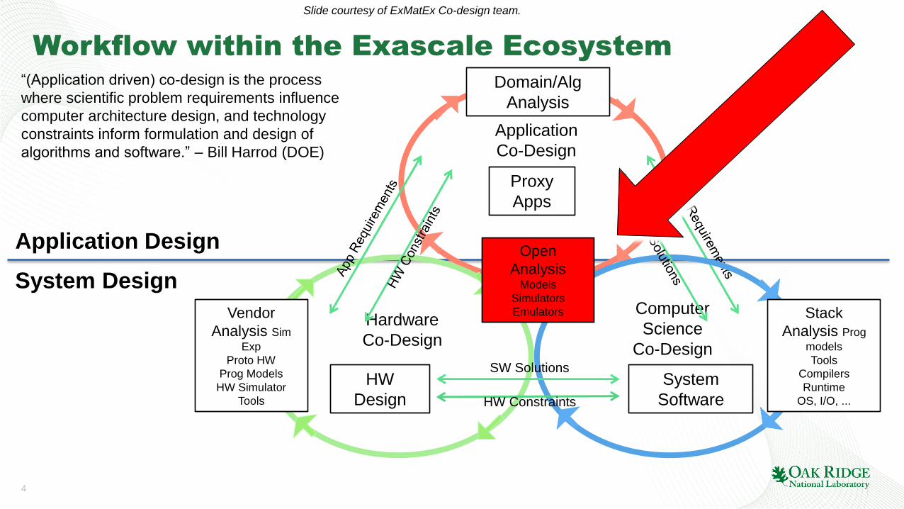
Aspen allows Multiresolution Modeling

Distributed Scientific Workflows

HPC System

Nodes

Wide-Area Networking, Files, Many HPC systems,

and Archives

Computation, Memory, Communication, IO

Computation, Memory, Threads

Scenario Scope

Scale

Node Scale Modeling with COMPASS

12

COMPASS System Overview

• Detailed Workflow of the COMPASS Modeling Framework

source code Input Program

Analyzer

Aspen machine

model

OpenARC IR with

Aspen annotations Aspen IR Generator

ASPEN IR

Aspen IR

Postprocessor

Aspen application

model Aspen

Performance

Prediction Tools

Program

characteristics

(flops, loads, stores,

etc.)

Runtime prediction

Optional feedback for advanced users

Other program

analysis

S. Lee, J.S. Meredith, and J.S. Vetter, “COMPASS: A Framework for Automated Performance Modeling and Prediction,” in ACM

International Conference on Supercomputing (ICS). Newport Beach, California: ACM, 2015, 10.1145/2751205.2751220.

15

MM example generated from COMPASS

16

Input MatMul Code Annotated to Use an Alternative

Algorithm

int N = 1024;

#pragma aspen control execute flops(N^2.372, traits(sp)) \

stores(N*N*floatS:to(A):traits(stride(1))) \

loads(N*N*floatS:from(B):traits(stride(1)), ...) …

void matmul(float * A, float * B, float * C) {

... //the original function body is here.

} //end of matmul()

int main()

{

... //the original main code is here.

}

• The original MatMul code uses a simple algorithm with O(N3) load operations.

• The new Aspen directive overrides the result produced by the analysis framework for the matmul() function

to use the Coppersmith-Winograd algorithm that requires only O(N2.372) operations, generating a new

Aspen application model without rewriting the input program.

17

Annotation Overhead

Benchmark Name Lines of Code Lines of Annotation Annotation Overhead

(%) JACOBI 241 2 0.8

MATMUL 128 1 0.7

SPMUL 423 10 2.3

LAPLACE2D 210 7 3.3

CG 1511 10 0.6

EP 759 9 1.1

BACKPROP 1074 4 0.3

BFS 435 16 3.6

CFD 752 9 1.1

HOTSPOT 525 11 2.0

KMEANS 1822 11 0.6

LUD 421 6 1.4

NW 478 8 1.7

SRAD 550 12 2.1

LULESH 3743 125 3.3

18

Example: LULESH (10% of 1 kernel)

kernel IntegrateStressForElems { execute [numElem_CalcVolumeForceForElems] { loads [((1*aspen_param_int)*8)] from elemNodes as stride(1) loads [((1*aspen_param_double)*8)] from m_x loads [((1*aspen_param_double)*8)] from m_y loads [((1*aspen_param_double)*8)] from m_z loads [(1*aspen_param_double)] from determ as stride(1) flops [8] as dp, simd flops [8] as dp, simd flops [8] as dp, simd flops [8] as dp, simd flops [3] as dp, simd flops [3] as dp, simd flops [3] as dp, simd flops [3] as dp, simd stores [(1*aspen_param_double)] as stride(0) flops [2] as dp, simd stores [(1*aspen_param_double)] as stride(0) flops [2] as dp, simd stores [(1*aspen_param_double)] as stride(0) flops [2] as dp, simd loads [(1*aspen_param_double)] as stride(0) stores [(1*aspen_param_double)] as stride(0) loads [(1*aspen_param_double)] as stride(0) stores [(1*aspen_param_double)] as stride(0) loads [(1*aspen_param_double)] as stride(0) . . . . . .

- Input LULESH program: 3700 lines

of C codes

- Output Aspen model: 2300 lines of

Aspen codes

19

Model Validation

FLOPS LOADS STORES MATMUL 15% <1% 1%

LAPLACE2D 7% 0% <1%

SRAD 17% 0% 0%

JACOBI 6% <1% <1%

KMEANS 0% 0% 8%

LUD 5% 0% 2%

BFS <1% 11% 0%

HOTSPOT 0% 0% 0%

LULESH 0% 0% 0%

0% means that prediction fell between measurements from optimized

and unoptimized runs of the code.

20

Model Scaling Validation (LULESH)

1.E+07

1.E+08

1.E+09

1.E+10

1.E+11

10 20 30 40 50

Byte

s Sto

red

Edge Elements

Measured(Unoptimized)

AspenPrediction

Measured(Optimized)

21

Example Queries

Performance Modeling

for Distributed

Scientific Workflows

23

Aspen allows Multiresolution Modeling

Distributed Scientific Workflows

HPC System

Nodes

Wide-Area Networking, Files, Many HPC systems,

and Archives

Computation, Memory, Communication, IO

Computation, Memory, Threads

Scenario Scope

Scale

24

PANORAMA Overview

Infrastructure

Design

Model Validation

Workflow Execution

Simulation

Anomaly

Detection and

Diagnosis

Resource

Mapping and

Adaptation

ExoGENI

OLCF

NERSC

Viz

APS

HPSS

VDF

SNS ES

ne

t

Workflow

Pegasus Framework

Aspen Modeling Language

and System

Resources

Ra

w a

nd

Co

rre

late

d M

on

ito

rin

g D

ata

ESnet

testbed

E. Deelman, C. Carothers et al., “PANORAMA: An Approach to Performance Modeling and Diagnosis of Extreme Scale Workflows,” International Journal of

High Performance Computing Applications, (to appear), 2015,

25

Workflow:

ACME

Climate

Modeling

26

Workflow: SNS

27

Automatically Generate Aspen from Pegasus DAX;

Use Aspen Predictions to Inform/Monitor Decisions

28

Workflow Monitoring Dashboard – pegasus-dashboard

Status, statistics, timeline of jobs

Helps pinpoint errors

End-to-end Resiliency Design using

Aspen

31

Data Vulnerability Factor: Why a new metric and

methodology?

• Analytical model of resiliency that includes important features of architecture and application

– Fast

– Flexible

• Balance multiple design dimensions

– Application requirements

– Architecture (memory capacity and type)

• Focus on main memory initially

• Prioritize vulnerabilities of application data

L. Yu, D. Li et al., “Quantitatively modeling application resilience with the data vulnerability factor (Best Student Paper Finalist),” in

SC14: International Conference for High Performance Computing, Networking, Storage and Analysis. New Orleans, Louisiana:

IEEE Press, 2014, pp. 695-706, 10.1109/sc.2014.62.

32

DVF Defined

𝑁𝑒𝑟𝑟𝑜𝑟 = 𝐹𝐼𝑇 ∗ 𝑇 ∗ 𝑆𝑑

Hardware Failure Rate ( 𝐹𝐼𝑇 ) Execution Time ( 𝑇 ) Footprint Size ( 𝑆𝑑 )

Hardware Effects Number of Errors ( 𝑵𝒆𝒓𝒓𝒐𝒓 )

Hardware Access Pattern

Application Effects Number of Hardware Accesses ( 𝑵𝒉𝒂 )

𝑁ℎ𝑎 Hardware Access Pattern

Data Structure Vulnerability → 𝐷𝑉𝐹𝑑 = 𝑁𝑒𝑟𝑟𝑜𝑟 ∗ 𝑁ℎ𝑎

Application Vulnerability → 𝐷𝑉𝐹𝑎 = 𝐷𝑉𝐹𝑑𝑖𝑛𝑖=1

Hardware Access Pattern

Application Effects Number of Hardware Accesses ( 𝑵𝒉𝒂 ) We focus on a specific hardware

component, the main memory, in this work

Larger DVF indicates higher vulnerability, and vice versa

33

Implementing DVF

• Extend Aspen performance modeling language

• Specify memory access patterns

• Combine error rates with memory regions and performance

• Assign DVF to each application memory region, Sum for application

34

Workflow to calculate Data Vulnerability Factor

35

An Example of Aspen Program for DVF

procedure VM(A,B,C) for i 1, 1000 do C[i] C[i] + A[i*4] * B[i*8] end for end procedure

Pseudocode

kernel vecmul { execute mainblock2 [1] { flops [2*(n^3)] as sp, fmad, simd access {1000} from {matA} as stream(4,16) access {4000} from {matB} as stream(4,32) access {8000} from {matC} as stream(4,4) } }

Extended Aspen Statements

Resilience Statements: Footprint Sizes: Int: 16,000 Data Structures: Ident: matA Access Pattern: Stream Int: 4 Int: 16 Resilience Statements: Footprint Sizes: Int: 16,000 Data Structures: Ident: matA Access Pattern: Stream Int: 4 Int: 16 Resilience Statements: Footprint Sizes: Int: 16,000 Data Structures: Ident: matA Access Pattern: Stream Int: 4 Int: 16

Syntax Tree

Data structure A: Number of errors: 30,400 Number of memory accesses: 51 DVF: 105504e+06 …

Resilience Modeling Results

Extended

Parser

Extended

Complier

36

36

DVF Results Provides insight for balancing interacting factors

37

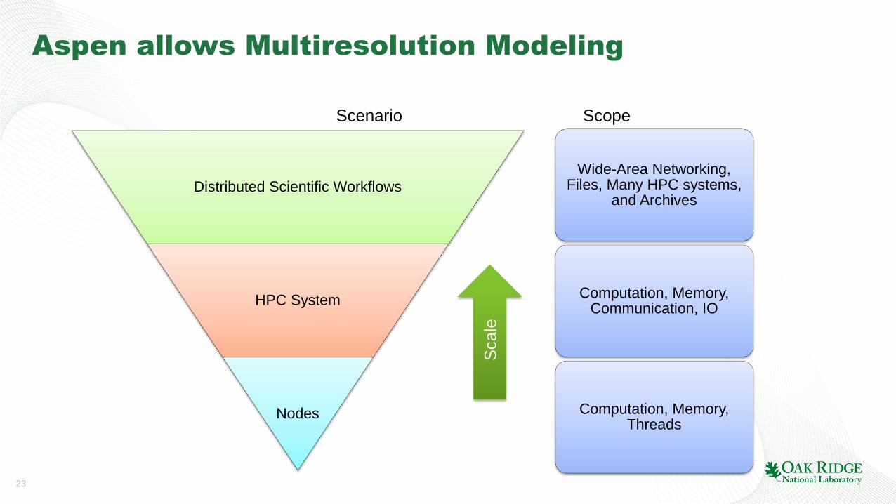
DVF: next steps

• Evaluated different architectures

– How much no-ECC, ECC, NVM?

• Evaluate software and applications

– ABFT

– C/R

– TMR

– Containment domains

– Fault tolerant MPI

• End-to-End analysis

– Where should we bear the cost for resiliency?

• Not everwhere!

37

39

Summary

• Our community has major challenges in HPC as we move to extreme scale – Power, Performance, Resilience, Productivity

– New technologies emerging to address some of these challenges • Heterogeneous computing

• Nonvolatile memory

– Not just HPC: Most uncertainty in at least two decades

• We need performance prediction and engineering tools now more than ever!

• Aspen is a tool for structured design and analysis – Co-design applications and architectures for performance, power, resiliency

– Automatic model generation

– Scalable to distributed scientific workflows

– DVF – a new twist on resiliency modeling

40

Acknowledgements

• Contributors and Sponsors

– Future Technologies Group: http://ft.ornl.gov

– US Department of Energy Office of Science

• DOE Vancouver Project: https://ft.ornl.gov/trac/vancouver

• DOE Blackcomb Project: https://ft.ornl.gov/trac/blackcomb

• DOE ExMatEx Codesign Center: http://codesign.lanl.gov

• DOE Cesar Codesign Center: http://cesar.mcs.anl.gov/

• DOE Exascale Efforts: http://science.energy.gov/ascr/research/computer-science/

– Scalable Heterogeneous Computing Benchmark team: http://bit.ly/shocmarx

– US National Science Foundation Keeneland Project: http://keeneland.gatech.edu

– US DARPA

– NVIDIA CUDA Center of Excellence

49

Notional Exascale Architecture Targets

(From Exascale Arch Report 2009)

System attributes 2001 2010 “2015” “2018”

System peak 10 Tera 2 Peta 200 Petaflop/sec 1 Exaflop/sec

Power ~0.8 MW 6 MW 15 MW 20 MW

System memory 0.006 PB 0.3 PB 5 PB 32-64 PB

Node performance 0.024 TF 0.125 TF 0.5 TF 7 TF 1 TF 10 TF

Node memory BW 25 GB/s 0.1 TB/sec 1 TB/sec 0.4 TB/sec 4 TB/sec

Node concurrency 16 12 O(100) O(1,000) O(1,000) O(10,000)

System size (nodes) 416 18,700 50,000 5,000 1,000,000 100,000

Total Node

Interconnect BW

1.5 GB/s 150 GB/sec 1 TB/sec 250 GB/sec 2 TB/sec

MTTI day O(1 day) O(1 day)

http://science.energy.gov/ascr/news-and-resources/workshops-and-conferences/grand-challenges/

Parallel I/O ??

50

Today’s Status

51

(Un-)Balanced Systems ??

System attributes 2001 2010 2014 est 2018 Summit/Titan

Name Seaborg3 Jaguar Titan SUMMIT

System peak 10 Tera 2 27 136 5.0

Power (MW) 0.8 6 9 10 1.1

Node main memory (GB) 16 38 512 13.5

System memory (PB) 0.006 0.3 0.7106 1.7408 2.4

Node Persistent Memory (GB) 800 inf

System Persistent Memory (PB) 2.72 inf

Node performance (TF) 0.024 0.125 1.4 0.5 7 40 28.6 1 10

Node memory BW 25 GB/s 0.1 TB/sec 1 TB/sec 0.4 TB/sec 4 TB/sec

Node concurrency 16 12 O(100) O(1,000) *POWER9s + *VOLTAs O(1,000) O(10,000)

System size (nodes) 416 18700 18700 50000 5000 3400 0.2 1000000 100000

Total Node Interconnect BW (GB/s) 1.5 GB/s 150 GB/sec 1 TB/sec 250 GB/sec 2 TB/sec

injection bandwidth per node (GB/s) 7.6 20 23 1.2

File system capacity (PB) 6 32 120 3.8

File system bandwidth (TB/s) 0.3 1 1 1.0

MTTI day O(1 day) O(1 day)

“2015” “2018”

200 1 Exaflop/sec

15 20

5 32-64

• Power is constant • 1/5 of the node count • Heterogeneous • I/O and NIC bandwidth has plateaued • NVM is new!