EXPLORATION OF SPECIAL CASES OF LAPLACETRANSFORMS

SARAMARGARET MLADENKA,TRI NGO,

KIMBERLY WARD,STEPHEN WILLIAMS

Abstract. First of all this paper discusses details of the gammafunction and explores some of its properties. Next, some of theproperties of Laguerre functions are shown as well as how thesefunctions relate to Laplace Transforms. In further study, differen-tial equations and properties of Laplace transform will be used tocalculate the Laplace transform of functions. Finally, many pointsof linear recursion relations will be explored and the Laplace trans-form will be used to solve them.

1. The Gamma Function

2. Laguerre Polynomials

Abstract. A polynomial p(x) in powers of x is a finite sum ofterms like

(2.1) p(x) =n∑

k=0

akxk

where k is a non-negative integer. The set of orthogonal polynomi-als contains polynomials that vanish when the product of any twodifferent ones, multiplied by a function w(x), called a weight func-tion, are integrated over a certain interval. This makes it possibleto expand an arbitrary function f(x) as a sum of the polynomials,each multiplied by a coefficient c(k), which is uniquely determinedby integration. The Laguerre polynomials are orthogonal on theinterval from 0 to ∞ with respect to the weight function w(x) =e−x . They also have many interesting properties and identitiessome of which involve differential operators, recursion and integra-tion. The Laplace transform is used to prove them here.

2.1. Laguerre’s equation. The equation

(2.2) ty′′ + (1− t)y′ + ny = 0,1

where n is a nonnegative intger, is known as Laguerre’s equation oforder n. This differential equation possesses the polynomial solution

(2.3) ln(t) =n∑k=0

n!(−1)ktk

(k!)2(n− k)!

The function ln(t) is known as the Laguerre polynomial of degree n.For n 6= m,

(2.4)

∫ ∞0

e−tln(t)lm(t)dt = 0.

2

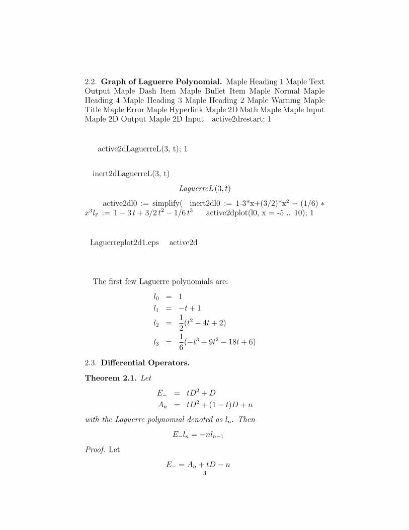
2.2. Graph of Laguerre Polynomial. Maple Heading 1 Maple TextOutput Maple Dash Item Maple Bullet Item Maple Normal MapleHeading 4 Maple Heading 3 Maple Heading 2 Maple Warning MapleTitle Maple Error Maple Hyperlink Maple 2D Math Maple Maple InputMaple 2D Output Maple 2D Input active2drestart; 1

active2dLaguerreL(3, t); 1

inert2dLaguerreL(3, t)

LaguerreL (3, t)

active2dl0 := simplify( inert2dl0 := 1-3*x+(3/2)*x2 − (1/6) ∗x3l3 := 1− 3 t+ 3/2 t2 − 1/6 t3 active2dplot(l0, x = -5 .. 10); 1

Laguerreplot2d1.eps active2d

The first few Laguerre polynomials are:

l0 = 1

l1 = −t+ 1

l2 =1

2(t2 − 4t+ 2)

l3 =1

6(−t3 + 9t2 − 18t+ 6)

2.3. Differential Operators.

Theorem 2.1. Let

E− = tD2 +D

An = tD2 + (1− t)D + n

with the Laguerre polynomial denoted as ln. Then

E−ln = −nln−1

Proof. Let

E− = An + tD − n3

Multiply both sides of the equation by ln.

E−ln = [An + tD − n]ln = −nln−1

tl′n − nln = −nln−1

−tl′n + nln = nln−1

Then, we proceed in transform space. So, apply the Laplace transform

to both sides of the equation with Ln = L{ln} = (s−1)n

sn+1 and simplify.

L{−tl′n + nln} = −[−(sLn(s)− ln(0))]′ + nLn

= −[−(Ln + sL′n)] + nLn

= Ln + sL′n + nLn

= sL′n + (1 + n)Ln

= s[(s− 1)n

sn+1]′ + (1 + n)

(s− 1)n

sn+1

= s[n(s− 1)n−1(s− 1)n+1 − (n+ 1)sn(s− 1)n

s2n+2]

+(1 + n)(s− 1)n

sn+1

=n(s− 1)n−1s2 − (n+ 1)(s− 1)ns

sn+2+ (1 + n)

(s− 1)ns

sn+2

=n(s− 1)n−1

sn−1

= nL{ln−1}(s)

�

Theorem 2.2. Let

EO = 2tD2 + (2− 2t)D − 1

An = tD2 + (1− t)D + n

Anln = 0

with the Laguerre polynomial denoted as ln. Then

EOln = −(2n+ 1)ln

Proof. Multiply An by 2

2An = 2tD2 + 2(1− t)D + 2n

2Anln = [2tD2 + 2(1− t)D + 2n]ln

0 = [2tD2 + 2(1− t)D + 2n]ln4

Add −(2n+ 1)ln to both sides of the equation and simplify

−(2n+ 1)ln = [2tD2 + 2(1− t)D + 2n]ln − (2n+ 1)ln

−(2n+ 1)ln = [2tD2 + 2(1− t)D − 1]ln

−(2n+ 1)ln = EOln

�

Theorem 2.3. Let

E+ = tD2 + (1− 2t)D + (t− 1)

An = tD2 + (1− t)D + n

Anln = 0

Then

E+ln = −(n+ 1)ln+1

Proof. Let

E+ = An − tD − (1− t− n)

Multiply by ln

E+ln = [An − tD − (1− t− n)]ln = −(n+ 1)ln+1

−tl′n − (1− t+ n)ln = −(n+ 1)ln+1

tl′n + (1− t+ n)ln = (n+ 1)ln+1

5

Then, we proceed in transform space. So, apply the Laplace transform

to both sides of the equation. Let Ln = L{ln} = (s−1)n

sn+1

L{tl′n + (1− t+ n)ln} = −(sLn(s)− ln(0))′ + (1 + n)Ln(s) + L′n(s)

= −(Ln + sL′n) + (1 + n)Ln + L′n= −(s− 1)L′n + nLn

= −(s− 1)[(s− 1)n

sn+1]′ + n[

(s− 1)n

sn+1]

= −(s− 1)[n(s− 1)n−1(s− 1)n+1 − (n+ 1)sn(s− 1)n

s2n+2]

+n[(s− 1)n

sn+1]

= −(s− 1)[n(s− 1)n−1(s− 1)s− (n+ 1)(s− 1)n

sn+2]

+n[(s− 1)n

sn+1]

= −(s− 1)[(s− 1)n−1[ns− (n+ 1)(s− 1)]

sn+2] +

n(s− 1)n

sn+1

=−(s− 1)n(n− s+ 1)

sn+2+n(s− 1)n

sn+1

=(s− 1)n(−n+ s− 1 + ns)

sn+2

=(s− 1)n(n+ 1)(s− 1)

sn+2

= (n+ 1)(s− 1)n+1

sn+2

= (n+ 1)L{ln+1}(s)

�

2.4. Lie Bracket.

Theorem 2.4. The Lie Bracket is defined as [A,B] = AB −BA. Let

EO = 2tD2 + (2− 2t)D − 1

E+ = tD2 + (1− 2t)D + (t− 1)

Then

[E0, E+] = −2E0

6

Proof. Let

[E0, E+] = −2E0 = E0E+ − E+E0(2.5)

E0E+ = 2tE′′

+ + (2− 2t)E′

+ − E+(2.6)

E+E0 = tE′′

0 + (1− 2t)E′

0 + (t− 1)E0(2.7)

and

−2E+ = −2tD2 + (−2 + 4t)D + (−2t+ 2)(2.8)

We must find the first and second derivatives of E0

E0 = 2tD2 + (2− 2t)D − 1

E′

0 = 2tD3 + (4− 2t)D2 − 3D

E′′

0 = 2tD4 + (6− 2t)D3 − 5D2

Now, we must find the first and second derivatives of E+

E+ = tD2 + (1− 2t)D + t− 1

Note that in the operator, t− 1 means (t− 1)f(t), so we have

d

dt[t− 1] =

d

dt[(t− 1)f(t)] = (t− 1)f

′(t) + f(t) = (t− 1)D + 1

Using that we get

E′

+ = tD3 + (2− 2t)D2 + (t− 3)D + 1

and

E′′

+ = tD4 + (3− 2t)D3 + (t− 5)D2 + 2D

Now, we substitute in the derivatives into (6) and (7)

E0E+ = 2tE′′

+ + (2− 2t)E′

+ − E+

= 2t[tD4 + (3− 2t)D3 + (t− 5)D2 + 2D] + (2− 2t)[tD3 + (2− 2t)D2 + (t− 3)D + 1]

−[tD2 + (1− 2t)D + t− 1]

= 2t2D4 +D3[6t− 4t2 + 2t− 2t2] +D2[2t2 − 10t+ 4− 8t+ 4t2 − t]+D[4t+ (2− 2t)(t− 3) + 2t− 1] + 2− 2t− t+ 1

= 2t2D4 + (−6t2 + 8t)D3 + (6t2 − 19t+ 4)D2 + (−2t2 + 14t− 7)D − 3t+ 37

E+E0 = tE′′

0 + (1− 2t)E′

0 + (t− 1)E0

= t[2tD4 + (6− 2t)D3 − 5D2] + (1− 2t)[2tD3 + (4− 2t)D2 − 3D]

+(t− 1)[2tD2 + (2− 2t)D − 1]

= 2t2D4 +D3[6t− 2t2 + 2t− 4t2] +D2[−5t+ 4− 10t+ 4t2 + 2t2 − 2t]

+D[6t− 3− 2t2 + 4t− 2]− t+ 1

= 2t2D4 + (−6t2 + 8t)D3 + (6t2 − 17t+ 4)D2 + (−2t2 + 10t− 5)D − t+ 1

Now, we plug everything into (5)

E0E+ − E+E0 = (2t2 − 2t2)D4 + [(−6t2 + 8t)− (−6t2 + 8t)]D3 + [(6t2 − 19t+ 4)

−(6t2 − 17t+ 4)]D2 + [(−2t2 + 14t− 7)− (−2t2 + 10t− 5)]D

−3t+ 3− (−t+ 1)

= −2tD2 + (4t− 2)D − 2t+ 2

Then using (5) and (8) we conclude that

[E0, E+] = −2E+

�

2.5. Properties of the Laguerre Function.

Theorem 2.5. Let

L{ln(at)} =n∑k=0

(nk)(−1)kakL{ tk

k!}

Then

L{ln(at)} =(s− a)n

sn+1when a ∈ <

Proof. We take the Laplace transform of the summation and simplify

L{ln(at)} =n∑k=0

(nk)(−1)kakL{ tk

k!}

=n∑k=0

(nk)(−1)kak1

sk+1

=1

sn+1

n∑k=0

(nk)(−a)ksn−k

following from the binomial theorem,

(s+ a)n =n∑k=0

(nk)aksn−k

8

we get

(s− a)n =n∑k=0

(nk)(−a)ksn−k

So,

L{ln(at)} =1

sn+1

n∑k=0

(nk)(−a)ksn−k =(s− a)n

sn+1

�

Theorem 2.6.

n∑k=0

(nk)aklk(t)(1− a)n−k = ln(at)

Proof. Apply the Laplace transform.

L{n∑k=0

(nk)aklk(t)(1− a)n−k} = L{ln(at)}

L{n∑k=0

(nk)aklk(t)(1− a)n−k} =n∑k=0

(nk)ak(s− 1)k

sk+1(1− a)n−k

=1

s

n∑k=0

(nk)ak(s− 1)k

sk(1− a)n−k

=1

s

n∑k=0

(nk)(a− a

s)k(1− a)n−k

using the binomial theorem, we get

1

s

n∑k=0

(nk)(a− a

s)k(1− a)n−k =

1

s(1− a+ a− a

s)n

=1

s(1− a

s)n

=1

s(s− as

)n

=(s− a)n

sn+1

L{n∑k=0

(nk)aklk(t)(1− a)n−k} = L{ln(at)}

9

By taking the inverse Laplace transform, we can conclude thatn∑k=0

(nk)aklk(t)(1− a)n−k = ln(at)

�

Theorem 2.7.∫ t

0ln(x)dx = ln(t)− ln+1(t)

Proof. We know that ln ∗ 1(t) =∫ t

0ln(x)dx

By the convolution theorem, we also know that

L{ln ∗ 1}(s) = L{ln}L{1}So we take the Laplace transform of ln and 1

L{ln}L{1} =1

s

(s− 1)n

sn+1

L{ln}L{1} = (1− s− 1

s)(s− 1)n

sn+1

SinceL{ln ∗ 1}(s) = L{ln}L{1}

we have

L{ln ∗ 1}(s) =(s− 1)n

sn+1− (s− 1)n+1

sn+2

L{ln ∗ 1}(s) = L{ln}(s)− L{ln+1}(s)Apply the inverse Laplace transform

ln ∗ 1 = ln(t)− ln+1(t)

By convolution, we can conlude that∫ t

0

ln(x)dx = ln(t)− ln+1(t)

�

Theorem 2.8.∫ t

0ln(x)lm(t− x)dx = lm+n(t)− lm+n+1(t)

Proof. We know that ln ∗ lm(t) =∫ t

0ln(x)lm(t− x)dx

By the convolution theorem, we also know that

L{ln ∗ lm}(s) = L{ln}L{lm}So we take the Laplace transform of ln and lm

L{ln}L{lm} =(s− 1)n

sn+1

(s− 1)m

sm+1

L{ln}L{lm} = (1− s− 1

s)(s− 1)n+m

sn+m+1

10

Since

L{ln ∗ lm}(s) = L{ln}L{lm}

we have

L{ln ∗ lm}(s) =(s− 1)n+m

sn+m+1− (s− 1)m+n+1

sm+n+2

L{ln ∗ lm}(s) = L{ln+m}(s)− L{ln+m+1}(s)

Apply the inverse Laplace transform

ln ∗ lm = lm+n(t)− lm+n+1(t)

By convolution, we can conlude that

∫ t

0

ln(x)lm(t− x)dx = lm+n(t)− lm+n+1(t)

�

Theorem 2.9. Recursion formula.

ln+1(t) =1

n+ 1[(2n+ 1− t)ln(t)− nln−1(t)]

11

Proof. Apply the Laplace transform to both sides of the equation and

simplify. Let Ln = L{ln} = (s−1)n

sn+1

L{ln+1(t)} = L{ 1

n+ 1[(2n+ 1− t)ln(t)− nln−1(t)]}

=1

n+ 1[(2n+ 1)Ln + L′n − nLn−1]

=1

n+ 1[(2n+ 1)[

(s− 1)n

sn+1] + [

(s− 1)n

sn+1]′ − n[

(s− 1)n−1

sn]]

=1

n+ 1[(2n+ 1)

(s− 1)n

sn+1+n(s− 1)n−1(s)n+1 − (n+ 1)sn(s− 1)n

s2n+2

−n(s− 1)n−1

sn]

=1

n+ 1[(2n+ 1)

(s− 1)n

sn+1+n(s− 1)n−1s− (n+ 1)(s− 1)n

sn+2− n(s− 1)n−1

sn]

=1

n+ 1[(2n+ 1)

(s− 1)n−1(s(s− 1))

sn+2+n(s− 1)n−1s− (n+ 1)(s− 1)n

sn+2

−ns2(s− 1)n−1

sn+2]

=1

n+ 1((s− 1)n−1

sn+2)[(2n+ 1)(s(s− 1)) + (n− s+ 1)− ns2]

=1

n+ 1((s− 1)n−1

sn+2)[(n+ 1)(s− 1)2]

=(s− 1)n−1

sn+2(s− 1)2

=(s− 1)n+1

sn+2

= L{ln+1(t)}

By applying the inverse Laplace transform we can conclude that

ln+1(t) =1

n+ 1[(2n+ 1− t)ln(t)− nln−1(t)]

�

3. Using Differential Equations to Compute LaplaceTransforms

3.1. Introduction. The Laplace transform of a function, F(t), is

f(s) =

∫ ∞0

e−atF (t)dt.

12

Theorem ?? and Table 1 are based on this definition.

Theorem 3.1. If f(s) = L{F (t)}, then

(1) sf(s)− F (0) = L{F ′(t)}(2) f ′(s) = L{−tF (t)}

Therefore, the following table is created.

f(s) F (t)x X

sx−X(0) X ′

s2x− sX(0)−X ′(0) X ′′

−x′ tX−sx′ − x tX ′

−s2x′ − 2sx+X(0) tX ′′

x′′ t2Xsx′′ + 2x′ t2X ′

s2x′′ + 4sx′ + 2x t2X ′′

Table 1. Basic Laplace Transforms

There are several other theorems that will also be useful to solveLaplace Transforms using differential equations.

Theorem 3.2. If X(t) ∼ Atα(α > −1) as t→ 0,

x(s) ∼ AΓ(α + 1)

sα+1as s→∞

Theorem 3.3. If X(t) ∼ Btβ(β > −1) as t→∞,

x(s) ∼ BΓ(β + 1)

sβ+1as s→ 0

3.2. Method 1. The first method used to compute Laplace Trans-forms uses Table ?? above to find the proper differential equations.

Theorem 3.4. The Laplace Transform of the zeroth-order Bessel Func-tion is the following:

L{J0(t)} =1√s2 + 1

and the Laplace Transform of the first-order Bessel Function is:

L{J1(t)} =

√s2 + 1− s√s2 + 1

13

Proof of Theorem ??. The Laplace Transform of the zeroth-order BesselFunction, denoted J0(t), is the solution of the differential equationtX ′′ + X ′ + tX = 0. By applying Table ?? to get the Laplace Trans-form, one can derive the equation s2x′−2sx+X(0)+sx−X(0)−x′ = 0.Putting this into the standard form of the differential equation gives:

x′ +s

s2 + 1x = 0.

In order to solve this differential equation, one has to find the Integrat-ing factor, which is defined by

I(t) = e

∫s

s2 + 1ds

By solving the integral and simplifying, the integrating factor is shownto be

√s2 + 1. Multiplying the differential equation by the integrating

factor gives√s2 + 1 x′+

√s2 + 1 s

s2+1x = 0, and integrating both sides

of the equation gives√s2 + 1 x = c, where c is the integration constant.

From this we can see that x(s) = c√s2+1

. According to Theorem ??,

c = 1 because x(s) ∼ 1/s as s→∞. Therefore,

L{J0(t)} =1√s2 + 1

.

In order to derive L{J1(t)}, the equality J ′0(t) = −J1(t) and Theorem?? are used by placing F (t) = J0(t) and F ′(t) = −J1(t). Then

L{J1(t)} =

√s2 + 1− s√s2 + 1

and the Theorem is proved.�

Theorem 3.5. The Laplace Transform of the function X(t) = sin a√t

can be stated as:

L{sin a√t} =

a√π

2s3/2e−a2

4s

Proof of Theorem ??. In order to prove this theorem, the equationX(t) = sin(a

√t) must be used. To find a differential equation to

solve for x(s) one must take the derivative twice and set the equationequal to zero to get the constants. Putting these 3 equations togetherto equal zero results in the differential equation 4tX ′′+2X ′+a2X = 0.Using the table, one can then take the Laplace transform of this equa-tion showing that 4(−s2x′ − 2sx + 4X(0)) + 2(sx −X(0)) + a2x = 0.

14

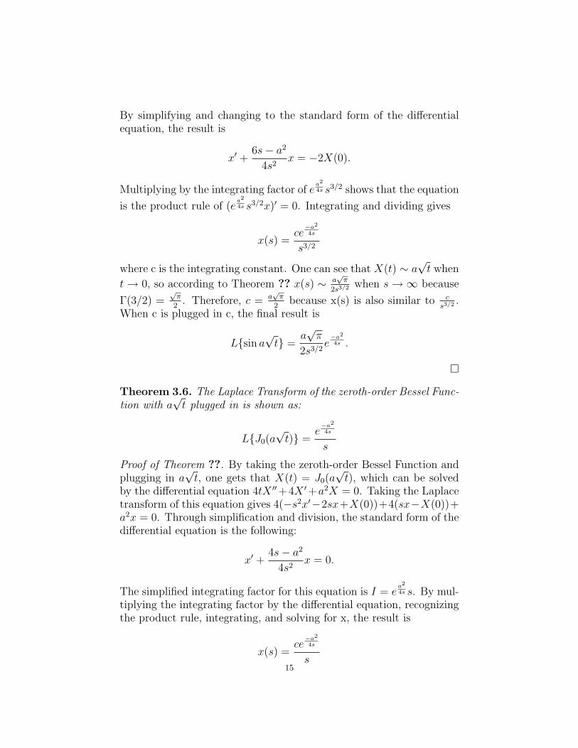
By simplifying and changing to the standard form of the differentialequation, the result is

x′ +6s− a2

4s2x = −2X(0).

Multiplying by the integrating factor of ea2

4s s3/2 shows that the equation

is the product rule of (ea2

4s s3/2x)′ = 0. Integrating and dividing gives

x(s) =ce−a2

4s

s3/2

where c is the integrating constant. One can see that X(t) ∼ a√t when

t→ 0, so according to Theorem ?? x(s) ∼ a√π

2s3/2 when s→∞ because

Γ(3/2) =√π

2. Therefore, c = a

√π

2because x(s) is also similar to c

s3/2 .When c is plugged in c, the final result is

L{sin a√t} =

a√π

2s3/2e−a2

4s .

�

Theorem 3.6. The Laplace Transform of the zeroth-order Bessel Func-tion with a

√t plugged in is shown as:

L{J0(a√t)} =

e−a2

4s

s

Proof of Theorem ??. By taking the zeroth-order Bessel Function andplugging in a

√t, one gets that X(t) = J0(a

√t), which can be solved

by the differential equation 4tX ′′+4X ′+a2X = 0. Taking the Laplacetransform of this equation gives 4(−s2x′−2sx+X(0))+4(sx−X(0))+a2x = 0. Through simplification and division, the standard form of thedifferential equation is the following:

x′ +4s− a2

4s2x = 0.

The simplified integrating factor for this equation is I = ea2

4s s. By mul-tiplying the integrating factor by the differential equation, recognizingthe product rule, integrating, and solving for x, the result is

x(s) =ce−a2

4s

s15

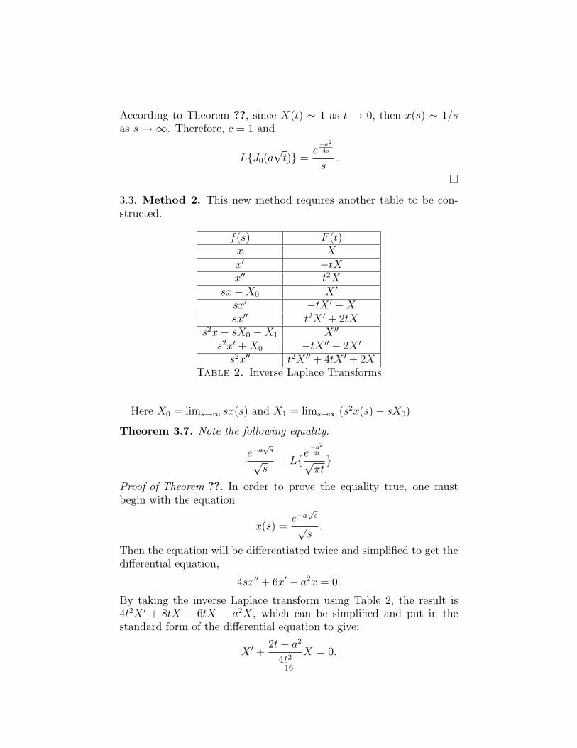
According to Theorem ??, since X(t) ∼ 1 as t → 0, then x(s) ∼ 1/sas s→∞. Therefore, c = 1 and

L{J0(a√t)} =

e−a2

4s

s.

�

3.3. Method 2. This new method requires another table to be con-structed.

f(s) F (t)x Xx′ −tXx′′ t2X

sx−X0 X ′

sx′ −tX ′ −Xsx′′ t2X ′ + 2tX

s2x− sX0 −X1 X ′′

s2x′ +X0 −tX ′′ − 2X ′

s2x′′ t2X ′′ + 4tX ′ + 2XTable 2. Inverse Laplace Transforms

Here X0 = lims→∞ sx(s) and X1 = lims→∞ (s2x(s)− sX0)

Theorem 3.7. Note the following equality:

e−a√s

√s

= L{e−a2

4t

√πt}

Proof of Theorem ??. In order to prove the equality true, one mustbegin with the equation

x(s) =e−a√s

√s.

Then the equation will be differentiated twice and simplified to get thedifferential equation,

4sx′′ + 6x′ − a2x = 0.

By taking the inverse Laplace transform using Table 2, the result is4t2X ′ + 8tX − 6tX − a2X, which can be simplified and put in thestandard form of the differential equation to give:

X ′ +2t− a2

4t2X = 0.

16

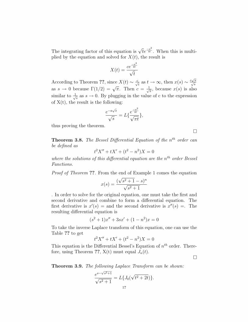
The integrating factor of this equation is√te−a2

4t . When this is multi-plied by the equation and solved for X(t), the result is

X(t) =ce−a2

4t

√t

According to Theorem ??, since X(t) ∼ c√t

as t→∞, then x(s) ∼ c√π√s

as s → 0 because Γ(1/2) =√π. Then c = 1√

π, because x(s) is also

similar to 1√s

as s→ 0. By plugging in the value of c to the expression

of X(t), the result is the following:

e−a√s

√s

= L{e−a2

4t

√πt},

thus proving the theorem.�

Theorem 3.8. The Bessel Differential Equation of the nth order canbe defined as

t2X ′′ + tX ′ + (t2 − n2)X = 0

where the solutions of this differential equation are the nth order BesselFunctions.

Proof of Theorem ??. From the end of Example 1 comes the equation

x(s) =(√s2 + 1− s)n√s2 + 1

. In order to solve for the original equation, one must take the first andsecond derivative and combine to form a differential equation. Thefirst derivative is x′(s) = and the second derivative is x′′(s) =. Theresulting differential equation is

(s2 + 1)x′′ + 3sx′ + (1− n2)x = 0

To take the inverse Laplace transform of this equation, one can use theTable ?? to get

t2X ′′ + tX ′ + (t2 − n2)X = 0

This equation is the Differential Bessel’s Equation of nth order. There-fore, using Theorem ??, X(t) must equal Jn(t).

�

Theorem 3.9. The following Laplace Transform can be shown:

es−√s2+1

√s2 + 1

= L{J0(√t2 + 2t)}.

17

This example displays a more difficult problem to solve and requiressupplementing Table 2 with additional entries.

f(s) F (t)x′′′ −t3Xs2x′′′ −t3X ′′ − 6t2X ′ − 6tX

Table 3. Additional Inverse Laplace Transforms

Proof of Theorem ??. To prove Theorem ??, one starts with the equa-tion

x(s) =es−√s2+1

√s2 + 1

.

The equation is then differentiated three times and the equations arecombined those equations to find the differential equation:

(s2 + 1)x′′′ − (3s2 − 5s+ 3)x′′ + (2s2 − 10s+ 7)x′ + (2s− 5)x = 0.

From Table 2 and Table 3, the inverse Laplace Transform of the equa-tion is (−t3−3t2−2t)X ′′+(−t2−12t−2)X ′+(−t3−3t2−3t−1)X = 0,which simplifies to

(t+ 1)(t2 + 2t)X ′′ + (t2 + 2t+ 2)X ′ + (t+ 1)3X = 0.

When a variable, y, is set equal to t2 + 2t, then this substitution canbe plugged into the equation to get 4yX ′′(y) + 4X ′(y) + X(y) = 0.By observation this differential equation is a form of the equation fromTheorem ?? where

L{J0(a√t)} =

e−a2

4s

s,

which solves the differential equation, 4tX ′′+ 4X ′+a2X = 0. Then bysubstituting y for t, this shows

es−√s2+1

√s2 + 1

= L{J0(√t2 + 2t)}.

�

These theorems demonstrate how to calculate Laplace transforms byusing differential equations. The properties of the Laplace Transformshown in the tables and solving the associated differential equationsmakes calculating Laplace transforms much easier.

18

4. Laplace Transform and Linear Recursion Relations

Abstract. In this part of the project we will be talking about howto use the Laplace transform to solve linear recursion relations.More specifically, we are looking at linear recursion relations oforder 2 which have the form:

an+2 + ban+1 + can = f(n),

where b and c are real numbers and f(n) is a known sequence. Ourgoal is to find a closed formula for an. We will see how the Laplacetransform could help us in solving these relations.

4.1. Introduction. In order to solve the linear recursion relations or-der 2: an+2 + ban+1 + can = f(n), we let y(t) = an, and f(t) = f(n)for n ≤ t < n+ 1 where n = 0, 1, 2, . . .. Now the relation becomes:

y(t+ 2) + by(t+ 1) + cy(t) = f(t)

Now take the Laplace transform of both sides, we have:

L{y(t+ 2)}+ bL{y(t+ 1)}+ cL{y(t)} = L{f(t)}(4.1)

In later sections, we will learn how to simplify the left side of Equation(??) in terms of Y (s) = L{y(t)}, and also how to compute the Laplacetransform of the right side, sometimes called the forcing function.After we have the closed form of Y (s), we will see how we could computethe Laplace inverse of that closed form to get the closed form of thesequence {an}.

4.2. Basic Laplace Transform Formulas.

4.2.1. Dealing with the left side. We will need the following propositionto simplify the left side of Equation (??):

Proposition 4.1. With notation as above we have

L{y(t+ 1)} = esY (s)− a0es(1− e−s)s

(4.2)

L{y(t+ 2)} = e2sY (s)− es(1− e−s)(a0es + a1)

s(4.3)

with Y (s) = L{y(t)}.19

Proof. 1 Let u = t+ 1, we have:

L{y(t+ 1)} =

∫ ∞0

e−sty(t+ 1)dt

= es∫ ∞

1

e−suy(u)du

= es∫ ∞

0

e−suy(u)du− es∫ 1

0

e−suy(u)du

= esY (s)− es∫ 1

0

e−sua0du

= esY (s)− a0es(1− e−s)s

using the fact that Y (t) = a0 for 0 ≤ t < 1. This proves Equation (??).Let u = t+ 2, we have:

L{y(t+ 2)} =

∫ ∞0

e−sty(t+ 2)dt

= e2s∫ ∞

2

e−suy(u)du

= e2s[∫ ∞

0

e−suy(u)du−∫ 1

0

e−suy(u)du

−∫ 2

1

e−suy(u)du

]= e2sY (s)− e2s

∫ 1

0

e−sua0du− e2s∫ 2

1

e−sua1du

= e2sY (s)− a0e2s(1− e−s)

s− a1e

2s(e−s − e−2s)

s

= e2sY (s)− es(1− e−s)(a0es + a1)

s

This proves Equation (??). �

Now we have successfully expressed L{y(t+ 2)} and L{y(t+ 1)} interms of Y (s) = L{y(t)}, so we could express the left side of (1) inform of Y (s).

4.2.2. Dealing with the right side. Next let’s see how we can deal withthe right side of Equation (??), finding the L{f(t)}. To do this, we

1These 2 identities and their proofs are taken from [?].20

need to use the Heaviside function hc(t) and on-off switch χ[a,b) thatare defined as followed:

hc(t) =

{0 if 0 ≤ t < c,

1 if c ≤ t.

χ[a,b) =

{1 if a ≤ t < b ,

0, elsewhere.

It is easy to prove that χ[a,b) = ha−hb. Also we will need the followingformula to compute the Laplace transform of our functions:

L{hc(t)} =e−sc

s

This formula and also its proof can be found in [?].Let’s first express f(t) in terms of Heaviside functions.

f(t) =

f(0) , if 0 ≤ t < 1 ,

f(1) , if 1 ≤ t < 2,...

f(n) , if n ≤ t < n+ 1,...

= f(0)χ[0,1) + f(1)χ[1,2) + . . .

= f(0) (h0 − h1) + f(1) (h1 − h2) + . . .

= f(0) + h1 (f(1)− f(0)) + h2 (f(2)− f(1)) + . . .

Now we have enough information to compute the Laplace transformfor f(t).

L{f(t)} =f(0)

s+

(f(1)− f(0)) e−s

s+

(f(2)− f(1)) e−2s

s+ . . .

=1

s

(f(0)(1− e−s) + e−sf(1)(1− e−s) + · · ·

)=

1− e−s

s·∞∑k=0

e−skf(k)

So we can write

(4.4) L{f(t)} =1− e−s

sG(s),

where G(s) =∑∞

k=0 e−skf(k). Below are some formulas regarding some

simple forcing functions.21

Proposition 4.2.

L{f(t) = k} =k

s

L{f(t) = rn, n ≤ t < n+ 1} =1− e−s

s(1− re−s)(4.5)

L{f(t) = n, n ≤ t < n+ 1} =e−s

s(1− e−s)Proof. From (??), we have:

G(s) = k∞∑i=0

e−si =k

1− e−s

Of course we need s > 0 to use that geometric series formula. Nowaccording to Equation (??), we will have L{f(t) = k} = k

s.

When f(n) = rn, with r is a constant. We have:

G(s) =∞∑k=0

e−skrk =∞∑k=0

(re−s)k =1

1− re−s

Again, we need to limit s such that: |re−s| < 1, so we could use thegeometric series formula. Now according to (??), we have:

L{f(t) = rn, n ≤ t < n+ 1} =1− e−s

s(1− re−s)When f(n) = n:

G(s) =∞∑k=0

ke−ks

=∞∑k=0

− d

ds

[e−ks

]= − d

ds

[∞∑k=0

e−ks

]

= − d

ds

[1

1− e−s

]=

e−s

(1− e−s)2

Again, from (??) we will have:

L{f(t) = n, n ≤ t < n+ 1} =e−s

s(1− e−s)22

�

Other kinds of forcing functions f(n) will be introduced later.

5. The Homogeneous Case

Here we want to consider a recursion relation of the form

an+2 − ban+1 + can = 0,

where b and c are real numbers. Such an equation is called homoge-nous. To get an idea of the general result let’s consider the followingexample. Let’s look at a very famous sequence, the Fibonacci sequence,which can be rewritten as:

an+2 − an+1 − an = 0,

where the initial conditions are a0 = 0 and a1 = 1. After setting upthe y(t) and taking the Laplace transform we have:

Y (s) =es(1− e−s)

s· 1

e2s − es − 1

Let r = es. Then we can write e2s−es−1 = r2−r−1 = (r−α)(r−β),

with α = 1+√

52

and β = 1−√

52

. Using partial fractions we have:

Y (s) =es(1− e−s)

s· 1

(es − α)(es − β)

=es(1− e−s)s(α− β)

·(

1

es − α− 1

es − β

)=

1− e−s

s(α− β)·(

1

1− αe−s− 1

1− βe−s

)By Proposition ??, we have

an =1

α− β(αn − βn)

=1√5·

[(1 +√

5

2

)n

−

(1−√

5

2

)n].

With this example as our guide we obtain the following theorem.

Theorem 5.1. The general solution of a linear recursion relation oforder 2: an+2 + ban+1 + can = 0 will be determined by its characteristicpolynomial x2 + bx+ c as following:

23

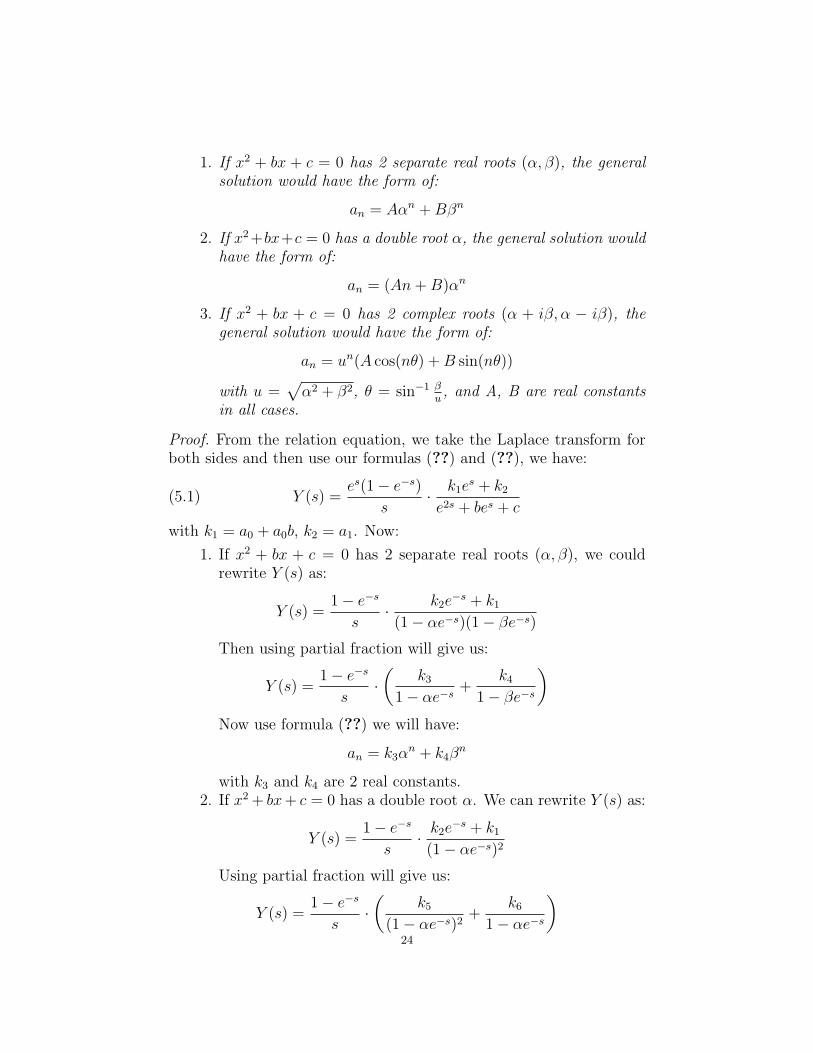
1. If x2 + bx + c = 0 has 2 separate real roots (α, β), the generalsolution would have the form of:

an = Aαn +Bβn

2. If x2 +bx+c = 0 has a double root α, the general solution wouldhave the form of:

an = (An+B)αn

3. If x2 + bx + c = 0 has 2 complex roots (α + iβ, α − iβ), thegeneral solution would have the form of:

an = un(A cos(nθ) +B sin(nθ))

with u =√α2 + β2, θ = sin−1 β

u, and A, B are real constants

in all cases.

Proof. From the relation equation, we take the Laplace transform forboth sides and then use our formulas (??) and (??), we have:

(5.1) Y (s) =es(1− e−s)

s· k1e

s + k2

e2s + bes + c

with k1 = a0 + a0b, k2 = a1. Now:

1. If x2 + bx + c = 0 has 2 separate real roots (α, β), we couldrewrite Y (s) as:

Y (s) =1− e−s

s· k2e

−s + k1

(1− αe−s)(1− βe−s)Then using partial fraction will give us:

Y (s) =1− e−s

s·(

k3

1− αe−s+

k4

1− βe−s

)Now use formula (??) we will have:

an = k3αn + k4β

n

with k3 and k4 are 2 real constants.2. If x2 + bx+ c = 0 has a double root α. We can rewrite Y (s) as:

Y (s) =1− e−s

s· k2e

−s + k1

(1− αe−s)2

Using partial fraction will give us:

Y (s) =1− e−s

s·(

k5

(1− αe−s)2+

k6

1− αe−s

)24

Now we need to use (??) to compute the function f(n) which

corresponds to the Laplace function of 1−e−s

s· 1

(1−αe−s)2. We

have:

1

(1− αe−s)2=

1

1− αe−s· 1

1− αe−s

=

(∞∑k=0

e−skαk

)·

(∞∑k=0

e−skαk

)=

(1 + αe−s + α2e−2s + . . .

)·(

1 + αe−s + α2e−2s + . . .)

= 1 + 2αe−s + 3α2e−2s + . . .

=∞∑k=0

e−sk(k + 1)αk

Therefore: f(n) = (n + 1)αn. Now using this to compute theLaplace transform of Y (s) will give us the general solution inthe form of:

an = (An+B)αn

3. If x2 + bx+ c = 0 has 2 complex roots (α+ iβ, α− iβ), with αand β are 2 real constants. From (??) we have:

Y (s) =1− e−s

s· k2e

−s + k1

(1− (α + iβ)e−s) (1− (α− iβ)e−s)

Using partial fraction gives us:

Y (s) =1− e−s

s·(

k7

1− (α + iβ)e−s+

k8

1− (α− iβ)e−s

)with:

k7 =k1β − (k2 + αk1)i

2β

k8 =k1β + (k2 + αk1)i

2β

Now use the Laplace inverse, we will have:

an = k7(α + iβ)n + k8(α− iβ)n

Note that we could express α± iβ as√α2 + β2(cos θ ± i sin θ)

with θ = sin−1 β√α2+β2

. Let’s call u =√α2 + β2. Use the De

25

Moivre’s formula we will have:

an = k7un (cos(nθ) + i sin(nθ)) + k8u

n (cos(nθ)− i sin(nθ))

= (k7 + k8)un cos(nθ) + iun sin(nθ)(k7 − k8)

= k1un cos(nθ) +

k2 + αk1

β· un sin(nθ)

an = un (A cos(nθ) +B sin(nθ))

�

5.1. Non-homogenous Recursion Relations. The following theo-rems are some theorems that gives us great insight into how to dealwith non-homogeneous cases.

Theorem 5.2. Let an,p be a fixed particular solution to the secondorder linear recursion relation

an+2 + ban+1 + can = f(n).

Then any other solution has the form an = an,h + an,p, for some homo-geneous solution an,h.

Proof. The theorem follows from linearity of the recursion relationequation. �

Theorem 5.3. Let an,p1 and an,p2 be particular solutions of the follow-ing relations respectively:

an+2 + ban+1 + can = f1(n)

an+2 + ban+1 + can = f2(n)

then a particular solution of the following relation

an+2 + ban+1 + can = f(n)

with f(n) = f1(n) + f2(n), will have the form of:

an,p = an,p1 + an,p2

Proof. Again the theorem follows from linearity of the recursion rela-tion equation. �

The biggest problem in solving a non-homogeneous case is to findthe particular solution. This will be discussed later in this section afterwe know some more formulas. For now let’s look at an example first.

26

5.2. Example. Find the closed form of an which is defined by thefollowing relation:

an+2 − 5an+1 + 6an = 4n, a0 = 0, a1 = 1.

After taking the Laplace transform and simplifying, we have:

Y (s) =1− e−s

2s·(

1

1− 4e−s− 1

1− 2e−s

)Taking the Laplace inverse will give us:

an =1

2(4n − 2n)

Note that if we want to use our theorem for this example, our generalhomogeneous solution have the form of:

an,h = c13n + c22

n

Later on we will know that our general particular solution in this caseis:

an,p = c34n

So our general solution would be:

an = c13n + c22

n + c34n

In this case, c1 happens to be zero. However, if we solve this relation inthe homogeneous case, we will have our solution to be: an = 3n − 2n.Now we can see that the existence of the forcing function does notonly add more terms to the general solution but it also changes thecoefficients of the terms in the homogeneous solution.

5.2.1. Dealing with the forcing function. Suppose f(n) is a forcing func-

tion with Laplace transform of the form F (s) = p1(e−s)sq1(e−s)

, where p1 and

q1 are polynomials. Here we will consider recursion relations of theform

an+2 + ban+1 + can = f(n).

After taking the Laplace transform for both sides and simplifying, wehave the following kind of equation:

(e2s + bes + c)Y (s) =p(e−s)

sq(e−s),

again, where p and q are polynomials. The characteristic polynomialcan be factored into 2 (or it can be one) factors (es − α) and (es − β),with α and β can be real or complex numbers. Also, since we do notlimit our numbers in the real set, our polynomial q(e−s) can also befactored into a product of terms in the form of (1 − re−s). Note that

27

the terms that we just mentioned are interchangeable. For example:(es − α) = es(1− αe−s). So we could rewrite our equation as:

Y (s) =1

s· p(e−s)∏

(1− rke−s)pe−sq

Now we can use partial fraction to break it into simple fractions like:

Y (s) =1

s·∑ ci

(1− rke−s)p

One might wonder what if we have terms like 1e−s ? Actually the term

e−s does appear sometimes in the denominator but when we get tothis stage, after we have everything in simple fractions type, we willnever have the fraction 1

e−s , which is es. We can prove this easily byusing the fact that Y (s) needs to go to zero when s goes to infinity.While all terms 1

s(1−re−s)p goes to zero when s goes to infinity, es

son

the other hand goes to infinity. Therefore, lims→∞ Y (s) 6= 0. So, bycontradiction, we have proved that we will never have the fraction 1

e−s

in our final step.Now all we need to do is to find the general formula for those kind

of fractions. Let H(n, p) be a function such that:

∞∑k=0

e−skH(k, p) =1

(1− re−s)p

We will use induction method to prove the following proposition:

Proposition 5.4.

(5.2) H(n, p) =rn

(p− 1)!·p−1∏k=1

(n+ k)

Proof. When p = 1, we need to prove that H(n, 1) = rn. This isobviously true according to our formula (??). Now suppose (??) istrue from 1 to p, we will need to prove that it’s also true for p+ 1. We

28

have:∞∑k=0

e−skH(k, p+ 1) =1

(1− re−s)p+1

=1

e−sp· ddr

[1

(1− re−s)p

]=

1

e−sp· ddr

[∞∑k=0

e−skH(k, p)

]

=1

p· ddr

[∞∑k=0

e−s(k−1)H(k, p)

]

=1

p·∞∑k=0

(e−s(k−1) · d

dr[H(k, p)]

)Now look at the formula (??), we have H(0, p) does not depend on thevalue of r. Therefore, its first derivative with respect to r is zero. Sonow in the summation, we just need k from 1 to ∞. But we want tomatch up with the left side of the equation, so we need to change it to0→∞. After doing this, we will have:

∞∑k=0

e−skH(k, p+ 1) =1

p·∞∑k=0

e−skd

dr[H(k + 1, p)]

H(n, p+ 1) =1

p· ddr

[H(n+ 1, p)]

=1

p· ddr

[rn+1

(p− 1)!·p−1∏k=1

(n+ 1 + k)

]

=(n+ 1)rn

p!·p−1∏k=1

(n+ 1 + k)

H(n, p+ 1) =rn

p!·

p∏k=1

(n+ k)

This means our formula (??) is also true for p + 1. By induction, wehave proved that (??) is true for all p > 0. �

Note that with the way we defined H(n, p), H(n, p) is not the Laplaceinverse function of the fraction 1

(1−re−s)p . Instead:

(5.3) H(n, p) = L−1{1− e−s

s· 1

(1− re−s)p}

29

Luckily, when we try to compute Y (s), we usually get terms that have

a common factor of 1−e−s

s. If we encounter some terms like 1

s(1−re−s)p

by itself, then we just need to multiply the numerator and denominatorby (1− e−s) and then use partial fraction to express 1

(1−e−s)(1−re−s)p in

terms of 11−e−s , and 1

(1−re−s)k , with 0 < k ≤ p. Finally, use the formula

of H(n, p) to compute the Laplace inverse of Y (s). Now let’s look atan example to see how we could use (??).

5.2.2. Example. Find the closed form of an which is defined by thefollowing relation:

an+2 − 5an+1 + 6an = n2n, a0 = 0, a1 = 1

First, let’s calculate the Laplace transform of the right side. From (??),we have:

L{f(t)} =1− e−s

s·∞∑k=0

e−skk2k

=1− e−s

s·

(∞∑k=0

e−sk(k + 1)2k −∞∑k=0

e−sk2k

)

=1− e−s

s·

(∞∑k=0

e−skH(k, 2)−∞∑k=0

(2e−s)k

)

=1− e−s

s·(

1

(1− 2e−s)2− 1

1− 2e−s

)Now take the Laplace transform for both sides of the relation equationand use our known formulas, we have:

Y (s)(e2s − 5es + 6) =1− e−s

s·(

1

(1− 2e−s)2− 1

1− 2e−s+ es

)Y (s) =

1− e−s

s·(

3

1− 3e−s− 5

2(1− 2e−s)− 1

2(1− 2e−s)3

)an = 3n+1 − 5

22n − 1

2H(n, 3){r = 2}

an = 3n+1 − 5.2n−1 − 1

4(n+ 1)(n+ 2)2n

an = 3n+1 − (n2 + 3n+ 12).2n−2

30

We can easily check the result and see that this is a correct formula foran. And now we have enough formulas to derive the following theoremabout particular solution.

Theorem 5.5. The particular solution of the second order linear recur-sion relation an+2+ban+1+can = g(n)rn, in which g(n) is a polynomialdegree k of n, will be determined as followed:

1. If the constant r does not match any roots (either real or com-plex) of the equation x2+bx+c = 0, then the particular solutionwould be in form of:

an,p = g∗(n)rn

with g∗(n) is a polynomial degree k of n.2. If the constant r matches one of the 2 separate roots of x2 +bx+ c = 0, the particular solution would be in form of:

an,p = g∗(n)rn

with g∗(n) is a polynomial degree k + 1 of n.3. If the constant r matches the double root of x2 + bx+ c = 0, the

particular solution would be in form of:

an,p = g∗(n)rn

with g∗(n) is a polynomial degree k + 2 of n.

Proof. Let’s look back at our formula (??) of H(n, p), and call theproduct

∏p−1k=1(n+ k) to be C(p). We have:

C(1) = 1

C(2) = n+ 1

C(3) = (n+ 1)(n+ 2)

C(4) = (n+ 1)(n+ 2)(n+ 3)

Note that C(p) is a polynomial degree p−1 of n. Next, we can expressg(n) in terms of C(i) with 1 ≤ i ≤ k + 1. That means:

g(n)rn =k+1∑j=1

cjH(n, j)

with cj are constants. Then we take the Laplace transform of g(n)rn,we would have the form of:

L{g(n)rn} =1− e−s

s·k+1∑j=1

cj(1− re−s)j

31

Note that the constants cj in this case does need to be the same asearlier equation. Therefore, our equation for particular solution willbe:

(5.4) Yp(s) =1− e−s

s·k+1∑j=1

cje−2s

(1− re−s)j(1− r1e−s)(1− r2e−s)

with r1, r2 are 2 roots of the characteristic polynomial: x2 +bx+c = 0.Note that we do not need to pay attention on how the fractions 1

1−r1e−s

and 11−r2e−s change because these 2 fractions (or one fraction 1

(1−r1e−s)2

in case of double root), will be combined into the homogeneous solutionformula. We will use h(r1, r2) to describe terms relating r1, r2. We justneed to pay attention on the power of 1 − re−s because these power(the highest power, to be more specific) will determine the degree ofthe polynomial g∗(n) after we take the Laplace inverse.

1. If r is different from both r1 and r2, after using partial fractionfor the right side of (??) we will have:

Yp(s) =1− e−s

s·

(h(r1, r2) +

k+1∑j=1

c∗j(1− re−s)j

)

Note that we would have the same form for Yp(s) if r1 and r2 arecomplex numbers. For more information about partial fraction,see chapter 2.2 of [?]. Taking the Laplace inverse will give us(note that the Laplace inverse of h(r1, r2) is combined into thehomogeneous solution):

an,p =k+1∑j=1

kjH(n, j)

Because H(n, k + 1) has the form of a product of rn and apolynomial degree k of n, we have:

an,p = g∗(n)rn

with g∗(n) is a polynomial degree k of n.2. If r equals one of the 2 separate roots (r, r1). Then (??) be-

comes:

Yp(s) =1− e−s

s·k+1∑j=1

cje−2s

(1− re−s)j+1(1− r1e−s)32

Note the highest power has increased by 1. After using partialfraction, we have:

Yp(s) =1− e−s

s·

(A

1− r1e−s+

k+2∑j=1

c∗j(1− re−s)j

)Taking the Laplace inverse will give us:

an,p =k+2∑j=1

kjH(n, j)

Again, use the formula of H(n, p), we will have:

an,p = g∗(n)rn

with g∗(n) is a polynomial degree k + 1 of n.3. If r equals the double root, meaning r = r1 = r2. From (??) we

have:

Yp(s) =1− e−s

s·k+1∑j=1

cje−2s

(1− re−s)j+2

Using partial fraction will give us:

Yp(s) =1− e−s

s·k+3∑j=1

c∗j(1− re−s)j

Note that in all 3 cases, the constants c∗j , kj are not the same.Now take the Laplace inverse we will have:

an,p =k+3∑j=1

kjH(n, j)

Therefore:

an,p = g∗(n)rn

with g∗(n) is a polynomial degree k + 2 of n.

�

5.2.3. Example. Let’s look back to the Example ??:

an+2 − 5an+1 + 6an = n2n

Our characteristic polynomial x2−5x+6 has 2 roots (2,3). Our constantr = 2 matches one of the roots. Therefore, our particular solutionwould be in form of:

an,p = g∗(n)2n

33

with g∗(n) is a polynomial degree 1 + 1 = 2 of n. Combine together wewould have the general solution:

an = c12n + c23

n + (c3n2 + c4n+ c5)2

n

We can see that this result agrees with the result we had in the example.

5.3. Forcing function involving sine and cosine. Our next goal isto deal with forcing functions that involve trigonometric functions sineand cosine.

5.3.1. Dealing with sine. Let’s look at a general relation:

an+2 + ban+1 + can = sin(kn)

First, let’s find the Laplace transform function of sin(kn). We will usethe following identity:

sin(ki+ k) + sin(ki− k) = 2 sin(ki) cos(k)

From (??), we have:

G(s) =∞∑i=1

e−si sin(ki)

2 cos(k)G(s) =∞∑i=1

e−si (2 sin(ki) cos(k))

=∞∑i=1

e−si (sin(ki+ k) + sin(ki− k))

=∞∑i=1

e−si sin (k(i+ 1)) +∞∑i=1

e−si sin (k(i− 1))

2 cos(k)G(s) =1

e−s·(G(s)− e−s sin(k)

)+ e−sG(s)

G(s) =sin(k)e−s

e−2s − 2 cos(k)e−s + 1

Therefore:

L{f(t) = sin(kn), n ≤ t < n+ 1} =1− e−s

s· sin(k)es

e2s − 2 cos(k)es + 1

Now starting from our relation equation, taking the Laplace trans-form for both sides, we will have:

Y (s) = L(s) +1− e−s

s· sin(k)es

(es − α)(es − β)(es − u)(es − v)

Y (s) = L(s) +Q(s)34

with (α, β) = (cos(k) + i sin(k), cos(k) − i sin(k)), which are 2 rootsof x2 − 2 cos(k)x + 1 = 0, and u, v are 2 roots of x2 + bx + c = 0(with x = es). The function L(s) corresponds to what we call thehomogenous solution, and the Q(s) is responsible for the particularsolution. Let’s calculate the Laplace inverse of Q(s):

Q(s) =sin(k)es(1− e−s)

s· 1

(es − α)(es − β)(es − u)(es − v)

=sin(k)es(1− e−s)

s·(

1c1(es − α)

+1

c2(es − β)+

1c3(es − u)

+1

c4(es − v)

)

=sin(k)(1− e−s)

s·(

1c1(1− αe−s)

+1

c2(1− βe−s)+

1c3(1− ue−s)

+1

c4(1− ve−s)

)

L−1{Q(s)} = sin(k) ·(αn

c1+βn

c2+un

c3+vn

c4

)L−1{Q(s)} = o(αn, βn) + p(un, vn)

with:

c1 = (α− β)(α− u)(α− v)c2 = (β − α)(β − u)(β − v)c3 = (u− α)(u− β)(u− v)c4 = (v − α)(v − β)(v − u)

Let’s examine the 2 terms of o(αn, βn). First of all, De Moivre’sformula gives us:

αn = (cos(k) + i sin(k))n = cos(kn) + i sin(kn)

βn = (cos(k)− i sin(k))n = cos(kn)− i sin(kn)

Next, when we simplify the coefficients of αn, and βn (2 denominators),we will see that they have similar forms: k1i+k2, and −k1i+k2. Usingthese facts we will have:

35

o(αn, βn) = sin(k) ·(

cos(kn) + i sin(kn)

k1i+ k2

+cos(kn)− i sin(kn)

−k1i+ k2

)=

sin(k)

k21 + k2

2

· (2k1 sin(kn) + 2k2 cos(kn))

o(αn, βn) = k3 sin(kn) + k4 cos(kn)

Combine this with p(un, vn), which has the form of k5un + k6v

n. Wenow know that our particular solution is in the form of: k3 sin(kn) +k4 cos(kn)+k5u

n+k6vn. Finally, combine this particular solution with

the homogenous solution, we will have our general solution:

an = c∗1un + c∗2v

n + c∗3 sin(kn) + c∗4 cos(kn)

Note that we have assumed that our characteristic polynomial functionhas 2 separate complex roots (u, v). The case when it has 1 double rootis very similar. Instead of having 2 terms 1

1−ue−s and 11−ve−s , we would

have 2 terms in form of 1(1−we−s)2

and 11−we−s , with w is the double root.

Therefore, using the formula for H(n, p) to take the Laplace inverse,our final general solution would be in form of:

an = (c1n+ c2)wn + c3 sin(kn) + c4 cos(kn)

Example. Let’s use our general solution formula to find the closed formfor the following sequence:

an+2 − 3an+1 + 2an = sin(n); a0 = 0, a1 = 1.

Our characteristic polynomial x2−3x+2 has two roots (2, 1). Therefore,our general solution would be:

an = c12n + c2 + c3 sin(n) + c4 cos(n)

From our relation equation, we could find a2 and a3. Then use theseresults with our initial conditions a0 and a1, we could have a systemequation to solve for ci. In fact, we could find that:

c1 = 1− sin(1)

4 cos(1)− 5

c2 =2 sin(2)− 5 sin(1)

(cos(1)− 1) · (8 cos(1)− 10)− 1

c3 =2 cos(1)− 1

8 cos(1)− 10

c4 =sin(2)− 3 sin(1)

(cos(1)− 1) · (10− 8 cos(1))36

Using these notation to express our constants would make it so difficultto check our formula. Instead, in order to check it, we could expressthem as approximate values:

an = (1.296)2n − 1.915− 0.0142 sin(n) + 0.619 cos(n)

Now we could easily check our formula, and we can see that this is acorrect formula for {an}.

5.3.2. Dealing with cosine. The method is exactly the same. There’sonly a little difference in computing the Laplace transform. We use thefollowing formula for computing G(s):

cos(ki+ k) + cos(ki− k) = 2 cos(ki) cos(k)

Now do exactly what we did to find G(s) for sine, we will have:

G(s){f(n) = cos(kn)} =1− cos(k)e−s

e−2s − 2 cos(k)e−s + 1

Therefore:

L{f(t) = cos(kn), n ≤ t < n+ 1} =1− e−s

s· 1− cos(k)e−s

e−2s − 2 cos(k)e−s + 1

Again, use the same method we used for sine, we will have our generalsolution to be the same as of sine:

an = c1un + c2v

n + c3 sin(kn) + c4 cos(kn)

Using the results we had for sine and cosine with the Theorem ??will give us the following theorem:

Theorem 5.6. The particular solution of a recursion relation of theform:

an+2 + ban+1 + can = f(n)

with f(n) is a linear combination of sin(kn) and cos(kn), in which kis a real constant, will have the form of:

an,p = A sin(kn) +B cos(kn)

with A, B are 2 real constants.

Proof. According to the Theorem, f(n) is a linear combination of sin(kn)and cos(kn). This means:

f(n) = c1 sin(kn) + c2 cos(kn)

Let g(n) = c1 sin(kn), h(n) = c2 cos(kn). First, consider the followingproperty: if an,g is the particular solution for the recursion relationan+2 + ban+1 + can = f(n), then the particular solution of the recursionrelation an+2 + ban+1 + can = pf(n), in which p is a real constant, will

37

be pan,g. This property is true by linearity of the recursion relation.Now use this property for g(n) and h(n), we will have their particularsolutions, respectively, to be: c1(c3 sin(kn)+c4 sin(kn)), c2(c5 sin(kn)+c6 cos(kn)). Then use the Theorem ??, we will have:

an,p = A sin(kn) +B cos(kn)

with A and B are 2 real constants. �

5.4. Conclusion. With all the formulas and theorems we have had sofar, we now have enough tool to deal with any linear recursion relationsof order 2 with the forcing function of the form:

f(n) =∑

gi(n)rni +∑

pi sin(kin) +∑

qi cos(cin)

with gi(n) are polynomials of n, and ri, pi, ki, qi, ci are constants.

Example. We could solve for the following relation using our knownformulas and theorems:

an+2 + ban+1 + can = (n+ 2)2n + (n2 + n+ 3)3n + 3 sin(2n) + cos(5n)

with b and c are 2 real constants.

Acknowledgements

The authors would like to thank Russ Frith for his help on thisproject in discussing and reviewing this work and Dr. Mark Davidsonwhose teaching and exposing made clear many of the points of thispaper. This paper was only possible through the VIGRE programat Louisiana State University with a grant from the National ScienceFoundation.

References

[1] Murray R. Spiegel, Schaum’s outline of theory and problems of Laplace Trans-forms, McGraw-Hill Book Company New York, 1965.

[2] William A. Adkins, Mark G. Davidson, Ordinary Differential Equations, to bepublished by Springer-Verlag.

[3] Richmond, D.E., Elementary Evaluation of Laplace Tansforms, in The AmericaMathematical Monthly, Williams College and Institute for Advanced Study,Mathematical Association of America, 1945, pp. 481–487.

[4] Bowman, Frank, Introduction to Bessel Functions Dover Publications, NewYork, 1958.

[5] Watson, G.N., A Treatise on the Theory of Bessel Functions, Second EditionCambridge University Press, Cambridge, 1995.

[6] Calvert, J.B. Laguerre Polynomials.14 November 2000. Web. 30 June 2009.http://mysite.du.edu/ jcalvert/math/laguerre.htm.

38

E-mail address: smlade1@tigers.lsu.edu, tmngo1@uno.edu, kaw205@msstate.edu,swilli13@xula.edu

39