EXPLOITING STRUCTURED DATA FOR MACHINE LEARNING ... · 3.1 Machine Learning for Textual Entailment...

UNIVERSITA DEGLI STUDI DI ROMA TOR VERGATADIPARTIMENTO DI INFORMATICA SISTEMI E PRODUZIONE

Dottorato di RicercaInformatica e Ingegneria dell’Automazione

Ciclo XXV

EXPLOITING STRUCTURED DATA FOR

MACHINE LEARNING: ENHANCEMENTS IN

EXPRESSIVE POWER AND COMPUTATIONAL

COMPLEXITY

Lorenzo Dell’Arciprete

Supervisor:Prof. Fabio Massimo Zanzotto

Rome, September 2013

Contents

1 Introduction 1

1.1 Machine Learning . . . . . . . . . . . . . . . . . . . . . . . . . . . . 2

1.2 Data Representation and Kernel Functions . . . . . . . . . . . . . . . 3

1.3 Thesis Contributions . . . . . . . . . . . . . . . . . . . . . . . . . . 4

1.4 Thesis Outline . . . . . . . . . . . . . . . . . . . . . . . . . . . . . . 6

2 Machine Learning and Structured Data 9

2.1 Classification in Machine Learning . . . . . . . . . . . . . . . . . . . 9

2.2 Kernel Machines and Kernel Functions . . . . . . . . . . . . . . . . . 10

2.3 Kernel Functions on Structured Data . . . . . . . . . . . . . . . . . . 14

2.3.1 Model-Driven Kernels . . . . . . . . . . . . . . . . . . . . . 15

2.3.1.1 Spectral Kernels . . . . . . . . . . . . . . . . . . . 15

2.3.1.2 Diffusion Kernels . . . . . . . . . . . . . . . . . . 16

2.3.2 Syntax-Driven Kernels . . . . . . . . . . . . . . . . . . . . . 17

2.3.2.1 Convolution Kernels . . . . . . . . . . . . . . . . . 17

2.3.2.2 String Kernels . . . . . . . . . . . . . . . . . . . . 18

2.3.2.3 Tree Kernels . . . . . . . . . . . . . . . . . . . . . 20

2.3.2.4 Graph Kernels . . . . . . . . . . . . . . . . . . . . 20

2.4 Tree Kernels: Potential and Limitations . . . . . . . . . . . . . . . . 22

2.4.1 Expressive Power . . . . . . . . . . . . . . . . . . . . . . . . 23

2.4.1.1 Extensions of the Subtree Feature Space . . . . . . 24

2.4.1.2 Other Feature Spaces . . . . . . . . . . . . . . . . 28

2.4.2 Computational Complexity . . . . . . . . . . . . . . . . . . . 32

iii

CONTENTS

3 Improving Expressive Power: Kernels on tDAGs 35

3.1 Machine Learning for Textual Entailment Recognition . . . . . . . . 36

3.2 Representing First-order Rules and Sentence Pairs as Tripartite Di-

rected Acyclic Graphs . . . . . . . . . . . . . . . . . . . . . . . . . . 40

3.3 An Efficient Algorithm for Computing the First-order Rule Space Kernel 44

3.3.1 Kernel Functions over First-order Rule Feature Spaces . . . . 45

3.3.2 Isomorphism between tDAGs . . . . . . . . . . . . . . . . . 47

3.3.3 General Idea for an Efficient Kernel Function . . . . . . . . . 50

3.3.3.1 Intuitive Explanation . . . . . . . . . . . . . . . . 51

3.3.3.2 Formalization . . . . . . . . . . . . . . . . . . . . 54

3.3.4 Enabling the Efficient Kernel Function . . . . . . . . . . . . 57

3.3.4.1 Unification of Constraints . . . . . . . . . . . . . . 58

3.3.4.2 Determining the Set of Alternative Constraints . . . 58

3.3.4.3 Determining the Set C∗ . . . . . . . . . . . . . . . 60

3.3.4.4 Determining Coefficients N(c) . . . . . . . . . . . 61

3.4 Worst-case Complexity and Average Computation Time Analysis . . . 63

3.5 Performance Evaluation . . . . . . . . . . . . . . . . . . . . . . . . . 66

4 Improving Computational Complexity: Distributed Tree Kernels 69

4.1 Preliminaries . . . . . . . . . . . . . . . . . . . . . . . . . . . . . . 71

4.1.1 Idea . . . . . . . . . . . . . . . . . . . . . . . . . . . . . . . 71

4.1.2 Description of the Challenges . . . . . . . . . . . . . . . . . 73

4.2 Theoretical Limits for Distributed Representations . . . . . . . . . . 77

4.2.1 Existence and Properties of Function f . . . . . . . . . . . . 77

4.2.2 Properties of the Vector Space . . . . . . . . . . . . . . . . . 80

iv

CONTENTS

4.3 Compositionally Representing Structures as Vectors . . . . . . . . . . 83

4.3.1 Structures as Distributed Vectors . . . . . . . . . . . . . . . . 83

4.3.2 An Ideal Vector Composition Function . . . . . . . . . . . . 85

4.3.3 Proving the Basic Properties for Compositionally-obtained Vec-

tors . . . . . . . . . . . . . . . . . . . . . . . . . . . . . . . 86

4.3.4 Approximating the Ideal Vector Composition Function . . . . 88

4.3.4.1 Transformation Functions . . . . . . . . . . . . . . 88

4.3.4.2 Composition Functions . . . . . . . . . . . . . . . 90

4.3.4.3 Empirical Analysis of the Approximation Properties 91

4.4 Approximating Traditional Tree Kernels with Distributed Trees . . . . 98

4.4.1 Distributed Collins and Duffy’s Tree Kernels . . . . . . . . . 99

4.4.1.1 Distributed Tree Fragments . . . . . . . . . . . . . 99

4.4.1.2 Recursively Computing Distributed Trees . . . . . 100

4.4.2 Distributed Subpath Tree Kernel . . . . . . . . . . . . . . . . 102

4.4.2.1 Distributed Tree Fragments for the Subpath Tree Ker-

nel . . . . . . . . . . . . . . . . . . . . . . . . . . 102

4.4.2.2 Recursively Computing Distributed Trees for the Sub-

path Tree Kernel . . . . . . . . . . . . . . . . . . . 103

4.4.3 Distributed Route Tree Kernel . . . . . . . . . . . . . . . . . 106

4.4.3.1 Distributed Tree Fragments for the Route Tree Kernel 106

4.4.3.2 Recursively Computing Distributed Trees for the Route

Tree Kernel . . . . . . . . . . . . . . . . . . . . . 107

4.5 Evaluation and Experiments . . . . . . . . . . . . . . . . . . . . . . 109

4.5.1 Trees for the Experiments . . . . . . . . . . . . . . . . . . . 109

v

CONTENTS

4.5.1.1 Linguistic Parse Trees and Linguistic Tasks . . . . . 109

4.5.1.2 Artificial Trees . . . . . . . . . . . . . . . . . . . . 110

4.5.2 Complexity Comparison . . . . . . . . . . . . . . . . . . . . 111

4.5.2.1 Analysis of the Worst-case Complexity . . . . . . . 111

4.5.2.2 Average Computation Time . . . . . . . . . . . . . 112

4.5.3 Experimental Evaluation . . . . . . . . . . . . . . . . . . . . 112

4.5.3.1 Direct Comparison . . . . . . . . . . . . . . . . . . 113

4.5.3.2 Task-based Experiments . . . . . . . . . . . . . . . 115

5 A Distributed Approach to a Symbolic Task: Distributed Representation

Parsing 123

5.1 Distributed Representation Parsers . . . . . . . . . . . . . . . . . . . 124

5.1.1 The Idea . . . . . . . . . . . . . . . . . . . . . . . . . . . . 125

5.1.2 Building the Final Function . . . . . . . . . . . . . . . . . . 126

5.1.2.1 Sentence Encoders . . . . . . . . . . . . . . . . . . 127

5.1.2.2 Learning Transformers with Linear Regression . . . 129

5.2 Experiments . . . . . . . . . . . . . . . . . . . . . . . . . . . . . . . 130

5.2.1 Experimental Set-up . . . . . . . . . . . . . . . . . . . . . . 131

5.2.2 Parsing Performance . . . . . . . . . . . . . . . . . . . . . . 133

5.2.3 Kernel-based Performance . . . . . . . . . . . . . . . . . . . 136

5.2.4 Running Time . . . . . . . . . . . . . . . . . . . . . . . . . 138

6 Conclusions and Future Work 141

6.1 Future Work . . . . . . . . . . . . . . . . . . . . . . . . . . . . . . . 144

vi

List of Tables

3.1 Comparative performances of Kmax and K . . . . . . . . . . . . . . 67

4.1 Relation between d, m and ε . . . . . . . . . . . . . . . . . . . . . . 80

4.2 Dot product between two sums of k random vectors, with h vectors in

common . . . . . . . . . . . . . . . . . . . . . . . . . . . . . . . . . 81

4.3 Computational time and space complexities for several tree kernel tech-

niques . . . . . . . . . . . . . . . . . . . . . . . . . . . . . . . . . . 111

4.4 Spearman’s correlation of DTK values with respect to TK values . . . 114

4.5 Spearman’s correlation of SDTK values with respect to STK values . 115

4.6 Spearman’s correlation of RDTK values with respect to RTK values . 116

5.1 Pseudo f-measure of the DRP s and the DSP on the non-lexicalized

data sets . . . . . . . . . . . . . . . . . . . . . . . . . . . . . . . . . 134

5.2 Pseudo f-measure of theDRP3 and theDSPlex on the lexicalized data

sets . . . . . . . . . . . . . . . . . . . . . . . . . . . . . . . . . . . 134

5.3 Spearman’s Correlation between the oracle’s vector space and the sys-

tems’ vector spaces . . . . . . . . . . . . . . . . . . . . . . . . . . . 136

vii

List of Figures

2.1 Routes in trees: an example . . . . . . . . . . . . . . . . . . . . . . . 30

3.1 A simple rule and a simple pair as a graph . . . . . . . . . . . . . . . 43

3.2 Two tripartite DAGs . . . . . . . . . . . . . . . . . . . . . . . . . . . 45

3.3 Simple non-linguistic tDAGs . . . . . . . . . . . . . . . . . . . . . . 51

3.4 Intuitive idea for the kernel computation . . . . . . . . . . . . . . . . 52

3.5 Algorithm for computing LC for a pair of nodes . . . . . . . . . . . . 59

3.6 Algorithm for computing C∗ . . . . . . . . . . . . . . . . . . . . . . 61

3.7 Comparison of the execution times . . . . . . . . . . . . . . . . . . . 64

4.1 Map of the used spaces and functions . . . . . . . . . . . . . . . . . 72

4.2 A sample tree . . . . . . . . . . . . . . . . . . . . . . . . . . . . . . 84

4.3 Norm of the vector obtained as combination of different numbers of

basic random vectors . . . . . . . . . . . . . . . . . . . . . . . . . . 92

4.4 Dot product between two combinations of basic random vectors, iden-

tical apart from one vector . . . . . . . . . . . . . . . . . . . . . . . 94

4.5 Variance for the values of Fig. 4.4 . . . . . . . . . . . . . . . . . . . 96

4.6 Tree Fragments for Collins and Duffy (2002)’s tree kernel . . . . . . 99

4.7 Tree Fragments for the subpath tree kernel . . . . . . . . . . . . . . . 103

4.8 Tree Fragments for the Route Tree Kernel . . . . . . . . . . . . . . . 106

4.9 Computation time of FTK and DTK . . . . . . . . . . . . . . . . . . 113

4.10 Performance on Question Classification task of TK, DTK� andDTK�117

4.11 Performance on Question Classification task of STK, SDTK� and

SDTK� . . . . . . . . . . . . . . . . . . . . . . . . . . . . . . . . 118

ix

LIST OF FIGURES

4.12 Performance on Question Classification task of RTK, RDTK� and

RDTK� . . . . . . . . . . . . . . . . . . . . . . . . . . . . . . . . 119

4.13 Performance on Recognizing Textual Entailment task of TK, DTK�

and DTK� . . . . . . . . . . . . . . . . . . . . . . . . . . . . . . . 120

4.14 Performance on Recognizing Textual Entailment task of STK, SDTK�

and SDTK� . . . . . . . . . . . . . . . . . . . . . . . . . . . . . . 121

4.15 Performance on Recognizing Textual Entailment task ofRTK,RDTK�

and RDTK� . . . . . . . . . . . . . . . . . . . . . . . . . . . . . . 122

5.1 “Parsing” with distributed structures in perspective . . . . . . . . . . 125

5.2 Subtrees of the tree t in Fig. 5.1 . . . . . . . . . . . . . . . . . . . . 127

5.3 Processing chains for the production of the distributed trees . . . . . . 132

5.4 Topology of the resulting spaces derived with the three different methods137

5.5 Performances with respect to the sentence length . . . . . . . . . . . 138

x

1Introduction

Learning, like intelligence, covers such a broad range of processes that it is difficult

to define it precisely. Zoologists and psychologists study learning in animals and hu-

mans, while computer scientists’ concern is about learning in machines. There are

several parallels between human and machine learning. Certainly, many techniques in

machine learning derive from the efforts of psychologists to make more precise theo-

ries of animal and human learning through computational models. It seems likely also

that the concepts and techniques being explored by researchers in machine learning

may illuminate certain aspects of biological learning.

With regard to machines, we might say that a machine learns whenever it changes

its structure, program, or data, based on its inputs or in response to external informa-

tion, in such a manner that its expected future performance improves. To put it in more

formal terms, “a computer program is said to learn from experience E with respect to

some class of tasks T and performance measure P, if its performance at tasks in T, as

measured by P, improves with experience E”(Mitchell, 1997). Some of these changes,

such as the addition of a record to a database, fall comfortably within the field of other

disciplines and may not necessarily be defined as learning. But, for example, when the

performance of a speech-recognition machine improves after hearing several samples

of a person’s speech, we feel quite justified to say that the machine has learned.

1

Chapter 1. Introduction

1.1 Machine Learning

There are several reasons why machine learning is important. Some of these are the

following.

• Some tasks cannot be defined well except by example, meaning that we might be

able to specify input-output pairs but not a concise relationship between inputs

and desired outputs. We would like machines to be able to adjust their internal

structure to produce correct outputs for a large number of sample inputs and thus

suitably constrain their input-output function to approximate the relationship im-

plicit in the examples, so that it could be applied to new cases as well.

• It is possible that hidden among large piles of data are important relationships

and correlations. Machine learning methods can often be used to extract these

relationships (Data Mining).

• Human designers often produce machines that do not work as well as desired in

the environments in which they are used. In fact, certain characteristics of the

working environment might not be completely known at design time. Machine

learning methods can be used for on-the-job improvement of existing machine

designs.

• The amount of knowledge available about certain tasks might be too large for ex-

plicit encoding by humans. Machines that learn this knowledge gradually might

be able to capture more of it than humans would want to write down.

• Environments change over time. Machines that can adapt to a changing environ-

ment would reduce the need for constant redesign.

2

1.2. Data Representation and Kernel Functions

• New knowledge about tasks is constantly being discovered by humans. Vocabu-

laries change. There is a constant stream of new events in the world. Continuing

redesign of AI systems to conform to new knowledge is impractical, but machine

learning methods might be able to track much of it.

To better explain what machine learning is about, let us consider a simple but well-

known example. In mathematics and statistics, we encounter techniques that, given a

set of points, e.g.→xi, and the values associated with them, e.g. yi, attempt to derive

the function that best interpolates the relation φ(~x, y), for example by means of linear

or polynomial regression. These are the first examples of machine learning algorithms.

The case we want to focus on is when the output values of the target function are finite

and discrete; then the regression problem can be regarded as a classification problem.

1.2 Data Representation and Kernel Functions

In the interpolation example, the data is represented by points in a vector space. This is

the common setting for most machine learning algorithms, such as decision tree learn-

ers (Quinlan, 1993), Bayesian networks (John and Langley, 1995), support vector ma-

chines (Cristianini and Shawe-Taylor, 2000) or artificial neural networks (Aleksander

and Morton, 1995). In general, the data points represent some real world entities by

means of their peculiar features; as such, the vector spaces used to represent data are

called feature spaces. The issue of determining an adequate feature space in order to

apply some learning algorithm is central to the machine learning problem.

Establishing a feature vector representation for a data object is a concern that has

been largely studied, independently of its backlashes on the machine learning con-

text. A whole literature exists on the topic of distributed representations (Hinton et al.,

3


1986; Rumelhart and McClelland, 1986). Inspired by the inherently distributed mech-

anisms taking place in a human brain, these studies aim at analyzing the possibility of

representing symbolic information in a distributed form. This objective is particularly

interesting, and challenging, when considering structured data, such as strings, trees or

graphs. A distributed representation is then expected to preserve information about the

structure of the object, i.e. about how its components are composed to form the whole

object (Plate, 1994).

Kernel functions have emerged as an alternative to the explicit distributed repre-

sentation of symbolic data. An interesting class of learning algorithms, the kernel

machines (Muller et al., 2001), deal with data only in terms of pairwise similarities. A

kernel function k(oi, oj) is then a function performing an implicit mapping φ of ob-

jects oi, oj into feature vectors ~xi, ~xj , so that k(oi, oj) = φ(oi) · φ(oj) = ~xi · ~xj . By

keeping the target feature space implicit, kernel functions allow for the use of huge,

possibly infinite feature spaces, overcoming the troubles of producing and dealing with

the corresponding feature vectors. As such, kernel functions over structured data have

gained large popularity. Many of these functions have been proposed to model a wide

range of feature spaces, capturing structure information at different levels of detail (see

Chapter 2).

1.3 Thesis Contributions

The aim of this thesis is to analyze the limits and possible enhancements of machine

learning techniques used to exploit structured data. We will focus on the framework

of kernel functions, and in particular on its application to tree structures. Trees are

a fundamental type of structure, widely used to represent objects in a broad range of

4

1.3. Thesis Contributions

research fields, such as proteins in biology, HTML documents in computer security

and syntactic interpretations in natural language processing. The perspective of the

present work is mainly oriented towards natural language processing tasks, though the

techniques introduced are relevant and useful for the other research areas involving tree

structures as well.

The analysis of the state of the art highlights two major lines of evolution for tree

kernel techniques. The first one is aimed at exploring feature spaces different from

the original one by Collins and Duffy (2002). This is necessary in order to define

more expressive tree kernels, often tailoring new feature spaces to the specific needs

of particular tasks. The second line of research tries to tackle the limitations deriving

from the tree kernels computational complexity. Having a complexity quadratic in the

size of the involved trees, tree kernels can hardly be applied to very large data sets or

data instances. In this regard, optimizations are needed, possibly allowing for some

approximation of the kernel results.

Regarding tree kernel expressiveness, we propose a kernel able to deal with struc-

tures more complex than trees (Zanzotto and Dell’Arciprete, 2009; Zanzotto et al.,

2011). These structures, called tDAGs, are composed of two trees linked by a set of

intermediate nodes, acting as variable names. The proposed kernel implements the fea-

ture space of first order rules between trees. This kind of space is inspired by the com-

putational linguistics task of textual entailment recognition, where the data instances

are pairs of sentences, and the task is to determine if the first one entails the second at a

linguistic level. The sentence pairs are represented as pairs of syntactic trees, possibly

sharing a common set of terms or phrases, thus constituting a tripartite directed acyclic

graph (tDAG). Though it has been shown that a complete kernel on graphs is NP-hard

5


to compute, we present an efficient computation for the kernel on tDAGs.

We then introduce a framework for the efficient computation of tree kernels, allow-

ing for some degree of approximation. The distributed tree kernels framework (Zan-

zotto and Dell’Arciprete, 2011a, 2012; Dell’Arciprete and Zanzotto, 2013) is based on

the explicit representation of trees in a distributed form, i.e. as low-dimensional vec-

tors. As long as these distributed representations for trees are built according to certain

criteria, the kernel computation can be approximated by a simple dot product in the

final vector space. This drastically reduces the computation time for tree kernels, since

a linear time algorithm is proposed for the construction of distributed trees. It is shown

how such a framework can be applied to different instances of tree kernels, leaving

open the possibility of applying it to other kinds of kernels and structures as well.

Finally, an application of the distributed tree kernels is proposed, in the task of syn-

tactic parsing of sentences (Zanzotto and Dell’Arciprete, 2013). The distributed repre-

sentation parser is a way to short-circuit the expensive and error-prone parsing phase,

in processes that apply kernel learning methods to natural language sentences. Such a

parser can be trained to produce the final distributed representation for a syntactic tree,

without explicitly producing the symbolic one.

1.4 Thesis Outline

The thesis outline is as follows.

In Chapter 2 we introduce the kernel machines approach to machine learning and

explain the use of kernel functions. We then provide a survey of kernels over several

kinds of structured data. In particular, we analyze the importance and limitations of

tree kernel functions. We give a more detailed survey of tree kernels, focusing on the

6

1.4. Thesis Outline

two aspects of expressive power and computational complexity.

In Chapter 3 we present our kernel on tDAGs for tree pairs classification. We ex-

plain the significance of the introduced feature space, and show the efficient algorithm

used to compute the kernel. We report experimental results on the task of textual en-

tailment recognition.

In Chapter 4 we present the distributed tree kernels framework. We show its the-

oretical foundations and our proposed implementation. We perform a wide empirical

analysis of the degree of approximation introduced by the distributed tree kernel. Then,

we report experimental comparisons on the tasks of question classification and textual

entailment recognition.

In Chapter 5 we present the distributed representation parser. We explain the learn-

ing process for the parser and we report several experimental results measuring its

correlation with respect to traditional symbolic parsers.

In Chapter 6, finally, we draw some conclusions and we outline future research

directions.

7

2Machine Learning and Structured Data

As one of the peculiar activities of the human mind, the ability to learn is a fundamental

part of what can be defined as an artificial intelligence. The field of machine learning

includes many different approaches, whose common aim is to produce systems able to

accurately perform a task on new, unseen examples, after having trained on a learning

data set. In other words, the objective of a machine learning algorithm is to generalize

from experience. Several kinds of algorithms have been developed, usually divided into

categories depending on the degree of human or external support given to the machine

learning system, in the learning process or as a feedback to the system behavior.

2.1 Classification in Machine Learning

The task of classification is one of the most important among machine learning activi-

ties. At its broadest, the term could cover any context in which some decision or fore-

cast is made on the basis of currently available information. A classification procedure

is then some formal method for repeatedly making such judgments in new situations.

Considering a more restricted interpretation, the problem concerns the construction of

a procedure that will be applied to a sequence of cases, in which each new case must

be assigned to one of a set of pre-defined classes on the basis of observed attributes or

features. The construction of a classification procedure from a set of data for which the

9

Chapter 2. Machine Learning and Structured Data

true classes are known has also been called supervised learning (in order to distinguish

it from unsupervised learning, in which the classes are inferred from the data).

The approach of machine learning to classification problems is thus to determine

algorithms that take as input a set of conveniently annotated examples, and return as

output a program, written according to some specific format. The output program

should be generated in such a way that it performs as accurately as possible on the

training examples. The effectiveness of a machine learning technique could be assessed

according to the two following properties:

• generalization: the degree to which the generated program can be successfully

applied to new examples. It obviously depends on both the complexity of the

program and the number of training examples used to generate it;

• computational tractability: the ability to find a good program in a short time.

When this is not the case, it should be possible to determine a useful approxima-

tion, requiring a smaller computational effort.

Clearly it is difficult to satisfy both properties at the same time. In fact, a more complex

program, built on the basis of a large set of training examples, will guarantee a better

generalization, but may take a large amount of time to be written. On the other hand, a

simpler program, generated according to a small set of examples, can be delineated in

a short time, but will probably perform badly on a generalized case.

2.2 Kernel Machines and Kernel Functions

One of the most useful learning methods used for classification are the Support Vector

Machines (SVMs) (Cortes and Vapnik, 1995; Scholkopf, 1997). Suppose we are given

10

2.2. Kernel Machines and Kernel Functions

a set of data points, each belonging to one of two classes, and the goal is to decide

which class a new data point will be in. The approach of support vector machines is

to view a data point as a n-dimensional vector, and to look for a (n − 1)-dimensional

hyperplane such that it can separate the points belonging to the two classes. Such a

classification method is called a linear classifier.

It is then necessary to define a multidimensional space able to represent the relevant

characteristics of the data objects taken into consideration. Such a space is called a

feature space, and its modeling is fundamental in the construction of a good learning

mechanism. In fact, the ability to split the data points in classes depends on the features

selected to represent the objects as vectors. A too small number of features (i.e. of

dimensions in the feature space) could lead to inseparability of the data; but this could

happen even by considering a very large set of features, if the characteristics chosen are

irrelevant to the problem in question. At the opposite, a feature space with an extremely

high number of dimensions could pose tractability issues, and for some problems no

feature space at all can be found such that it allows linear separability of the data.

Assuming we can design an adequate feature space, there might be many hyper-

planes able to classify the data. However, we are additionally interested in finding out

if we can achieve maximum separation (margin) between the two classes. By this we

mean that the hyperplane should be picked so that the distance from the nearest data

points to the hyperplane itself is maximized. Now, if such a hyperplane exists, it is

clearly of interest and is known as the maximum-margin hyperplane, and such a linear

classifier is known as a maximum-margin classifier.

The simplest form of SVM is the algorithm known as Perceptron (Rosenblatt,

1958), that can be seen as an artificial version of the human brain neurons. The Per-

11


ceptron classification function is of the form:

f(~x) = sgn(~w · ~x+ b)

where ~w · ~x + b represents a simple hyperplane and the signum function divides the

data points in two sets: those that are above and those that are below the hyperplane.

The major advantage of making use of linear functions only is that, given a set of

training points, S = { ~x1, ..., ~xm}, each one associated with a classification label yi ∈

{+1,−1}, we can apply a learning algorithm that derives the vector ~w and the scalar b

of a separating hyperplane, provided that at least one exists.

Since we are interested in finding the maximum-margin hyperplane, it is possible

to demonstrate that the objective of learning is reduced to an optimization problem of

the form: min ||~w||

yi(~w · ~xi + b) ≥ 1 ∀~xi ∈ S

In real scenario applications, training data is often affected by noise due to several

reasons, e.g. classification mistakes of the annotators. These may cause the data not

to be separable by any linear function. Additionally, as we already pointed out, the

target problem itself may not be separable in the designed feature space. As a result,

the simplest version of SVM (called Hard Margin SVM), as described above, will fail

to converge. In order to solve such a critical aspect, a more flexible design is proposed

with Soft Margin Support Vector Machines. The main idea is that the optimization

problem is allowed to provide solutions that can violate a certain number of constraints.

Obviously, to be as much as possible consistent with the training data, the number of

such errors should be the lowest possible.

One of the most interesting properties we can observe about SVMs is that the gra-

12

2.2. Kernel Machines and Kernel Functions

dient ~w is obtained by a summation of vectors proportional to the examples ~xi. This

means that ~w can be written as a linear combination of training points, i.e.:

~w =

m∑i=1

αiyi ~xi

where the coefficients αi can be seen as the alternative coordinates for representing

the vector ~w in a dual space, whose dimensions are the training data vectors. This

also means that every scalar product between vector ~w and a data vector ~x can be

decomposed in a summation of scalar products between data vectors.

One of the most difficult tasks for applying machine learning is the features design.

Features should represent data in a way that allows learning algorithms to separate

positive from negative examples. In SVMs, features are used to build the vector rep-

resentation of data examples, and the scalar product between example pairs quantifies

how much they are similar (sometimes simply counting the number of common fea-

tures). Instead of encoding data in feature vectors, we may design kernel functions

(Vapnik, 1995) that provide such similarity between example pairs without using an

explicit feature representation.

In this way, a linear classifier algorithm can solve also a non-linear problem by

mapping the original non-linear observations into a higher-dimensional space, where

the linear classifier is subsequently used. This process, also known as the kernel trick,

makes a linear classification in the new space equivalent to non-linear classification in

the original space.

In the optimization problem used to learn SVMs, the feature vectors always appear

in a scalar product; consequently, the feature vectors ~xi can be replaced with the data

objects oi, by substituting the scalar product ~xi · ~xj with a kernel function k(oi, oj). The

initial objects oi can be mapped into the vectors ~xi by using a feature representation,

13


φ(.), so that ~xi · ~xj = φ(oi) · φ(oj) = k(oi, oj).

The idea of a feature extraction procedure φ : o → (x1, ..., xn) = ~x allows us to

define a kernel as a function k such that ∀~x, ~z ∈ X

k(~x, ~z) = φ(~x) · φ(~z)

where φ is a mapping from X to an (inner product) feature space.

Notice that, once we have defined a kernel function that is effective for a given

learning problem, we do not need to find explicitly which mapping φ it corresponds

to. It is enough to know that such a mapping exists. This is guaranteed by Mercer’s

theorem (Mercer, 1909), stating that any continuous, symmetric, positive semi-definite

kernel function k(x, y) can be expressed as a scalar product in a high-dimensional

space.

The use of kernel functions allows SVMs to solve non-linear classification prob-

lems. Learning algorithms, such as SVMs, building on kernel functions are called

kernel machines.

2.3 Kernel Functions on Structured Data

Real world tasks often deal with data that is not represented as mere attribute-value

tuples. Strings, trees and graphs are extensively used to represent different kinds of

objects, in several areas such as natural language processing, biology and computer

security. The application of machine learning methods to classification tasks in these

fields has led to a wide development of kernel functions able to deal with such kinds

of structured data. It should be noted that, by talking about kernels for structured data,

one could refer to two different families of kernel functions: model-driven kernels and

syntax-driven kernels (Gartner, 2003).

14

2.3. Kernel Functions on Structured Data

2.3.1 Model-Driven Kernels

Model-driven kernels are kernels defined on the structure of the instance space, such as

the spectral kernels and the diffusion kernels.

2.3.1.1 Spectral Kernels

Spectral kernels (Li et al., 2005) are a form of support to automatic learning method-

ologies based on the use of kernel functions. Having a set of n samples, a kernel matrix,

or Gram matrix, K can be defined as a matrix with dimensions n× n, whose element

Ki,j contains the value of the kernel function for samples i and j. Spectral kernels stem

from spectral graph theory, since their functioning is based on the analysis of kernel

matrices in terms of their characteristic properties, like their eigenvalues and eigenvec-

tors. These properties can be used, for example, for determining a clustering of the

samples, by finding some optimum cut in the graph whose adjacency matrix is given

by the kernel matrix.

Spectral kernels work as follows. Firstly, they may apply a transformation to the

n × n kernel matrix (i.e. consider the Laplacian matrix of the corresponding graph).

Then, they perform an eigen-decomposition of the transformed matrix, and use it to

extract feature vectors of length k for the n objects. Finally, the kernel is computed by

classic similarity measures over Rk.

New input, considered as a vector of original kernel values with respect to the

training examples, is firstly transformed in a manner dependent on the transformation

previously used, and then is projected onto the spectral embedding space given by the

training examples.

Following a similar principle, the Latent Semantic Kernel (Cristianini et al., 2002)

15


can be viewed as a specific instance of the spectral kernel framework. In this case,

starting from a generic kernel matrix, the LSK works by manipulating the kernel ma-

trices through Latent Semantic Indexing techniques (Deerwester et al., 1990), which

are successfully used in the context of Information Retrieval to capture semantic rela-

tions between terms and documents.

2.3.1.2 Diffusion Kernels

Diffusion kernels (Kondor and Lafferty, 2002) can be applied to data sets that can be

regarded as vertices of a graph (e.g. documents linked in the Web). The idea comes

from the equations used to describe the diffusion of heat through a medium. Diffusion

kernels are related to the Gaussian kernel over Rn, which gives a measure of similarity

according to the Gaussian function with parameter σ, as k(~x, ~z) = e−‖~x−~y‖2

2σ2 .

As a more generic approach, exponential kernels are defined by means of a Gram

matrix K = eβH = limt→∞

(I βHt

)t. β is a “bandwidth” parameter, of meaning

similar to parameter σ in Gaussian kernels, and H , the “generator”, is a symmetric

square matrix.

Diffusion kernels on graphs are obtained by choosing matrix H to represent the

structure of the considered graph. In particular, H is taken to be the negative of the

Laplacian matrix, i.e. its elements Hi,j are defined as −degree(vi) if i = j, 1 if

(vi, vj) ∈ E and 0 otherwise.

Intuitively, the diffusion kernel K(x, x′) represents the heat found at point x at

time tβ if all the heat of the system was concentrated in x′ at time 0. This is also

related to random walks on the graph, defining the probability distribution of finding the

walker in vertex x at some step, if starting at vertex x′. While random walks consider a

discrete series of steps, diffusion kernels can be seen as considering an infinite number

16


of infinitesimal steps. At each step the walker in vertex vi will take each of the edges

emanating from vi with fixed probability β and will remain in place with probability

1− degree(vi)β.

2.3.2 Syntax-Driven Kernels

Syntax-driven kernels are kernels defined on the structure of the instances. They deal

with instances belonging to families of structured data such as strings, trees and graphs.

Being the main focus of the present work, in the following sections and chapters, by

kernels on structured data we will always refer to syntax-driven kernels.

2.3.2.1 Convolution Kernels

The vast majority of kernels on structured data stem from the convolution kernel (Haus-

sler, 1999), whose key idea is to define a kernel on a composite object by means of

kernels on the parts of the objects. This originates from the assumption that often the

semantics of structured objects can be captured by a relation R between the object and

its parts.

Let x, x′ ∈ X be the composite objects and ~x, ~x′ ∈ X1×· · ·×XD be tuples of parts

of these objects. Given the relation R : (X1× · · · ×XD)×X , the decomposition R−1

can be defined as R−1(x) = {~x : R(~x, x)}. Then the convolution kernel is defined as:

kconv(x, x′) =

∑~x∈R−1(x), ~x′∈R−1(x′)

D∏d=1

kd(xd, x′d)

Convolution kernels are then a class of kernels that can be formulated in the above

way. Their advantage is that they are very general and can be applied to many different

problems. The work required to adapt the general formulation to a specific problem

17


consists in choosing an adequate relation R. Simpler and more complex kinds of de-

composition relations have been studied for structures such as strings, trees and graphs,

to define several kernels based on the general framework of the convolution kernel.

2.3.2.2 String Kernels

The traditional model for text classification is based on the bag-of-words representa-

tion, which associates a text with a vector indicating the number of occurrences of terms

in the text. Text similarity is then computed as a simple scalar product between these

vectors. Kernels on strings try to define a more sophisticated approach to the problem

of text classification, though they can be applied also to other sequences of symbols,

e.g. the amino acids describing a protein or the phonemes constituting spoken text.

The first kernel function defined on strings can be found in Lodhi et al. (2002), and it

is based on a notion of string similarity given by the number of common subsequences.

These subsequences need not be contiguous, but their relevance is weighted according

to the number of gaps occurring in the subsequence, so that the more gaps it contains,

the less weight it is given in the kernel function.

Consider a string to be a finite sequence of characters from a finite alphabet Σ. Then

Σn is the set of strings of length n and Σ∗ is the set of all strings, including the empty

string. Let |s| denote the length of string s = s1, ..., s|s|, and s[i] the subsequence of s

induced by the set of indices i. The total length l(i) of subsequence s[i] in s is defined

as i|i| − i1 + 1, where the indices in i are ordered so that 1 ≤ i1 < ... < i|i| ≤ |s|.

Then, the mapping φ underlying the string kernel can be defined for each element of

the feature space, i.e. the space of all possible substrings Σ∗. For any substring u, the

18


value of feature φu(s) is:

φu(s) =∑

i:u=s[i]

λl(i)

where λ ≤ 1 is a decay factor that penalizes long and gap-filled subsequences. Then,

the kernel between strings s and t is the inner product of the feature vectors for the two

strings, computing a weighted sum over all common subsequences:

k(s, t) =∑u∈Σ∗

φu(s)φu(t) =∑u∈Σ∗

∑i:u=s[i]

∑j:u=t[j]

λl(i)+l(j)

In Lodhi et al. (2002), a restricted formulation is given, considering as the feature space

only the subsequences of length n, i.e. Σn:

kn(s, t) =∑u∈Σn

φu(s)φu(t) =∑u∈Σn

∑i:u=s[i]

∑j:u=t[j]

λl(i)+l(j)

and an efficient recursive algorithm is given to reduce the computation complexity to

O(n|s||t|). Rousu and Shawe-Taylor (2005) introduce a further optimization, reducing

the complexity to O(n|M | log min(|s|, |t|)), where M = {(i, j)|si = tj} is the set of

characters matches in the two sequences.

Leslie et al. (2002) and Paass et al. (2002) use an alternative kernel in the context

of protein and spoken text classification, considering only contiguous substrings. A

string is then represented by the number of times each unique substring of length n

occurs in the sequence. This way of representing a string as its n-grams is also known

as the spectrum of a string. The kernel function is then simply the scalar product of

these representations, and can be computed in time linear in n and in the length of the

strings.

String kernels can also be seen as a specific instance of more generic sequence

kernels, where the symbols of the string are not characters but more complex objects,

19


even strings themselves. As an example, Bunescu and Mooney (2006) proposed a

subsequence kernel for the task of extracting relations among entities from texts. Their

kernel applies to sequences of objects taken from a set Σ× = Σ1 × Σ2 × ... × Σk,

where each object includes several features from feature sets Σ1,Σ2, ...,Σk, e.g. a

word, a POS tag, etc. Then, if we consider the set of all possible features Σ∪ =

Σ1 ∪ Σ2 ∪ ... ∪ Σk, a sequence u ∈ Σ∗∪ is a subsequence of sequence s ∈ Σ∗× if there

is a sequence of |u| indices i such that uk ∈ sik for all k = 1, ..., |u|.

2.3.2.3 Tree Kernels

The study of kernel functions for trees has been very popular and led to several different

tree kernel formulations. The differences among the various tree kernels are related

to both the feature spaces covered and the kind of trees considered (e.g. ordered or

unordered, labeled or unlabeled edges). Since they constitute the focus of this work,

an extensive overview of tree kernel functions can be found in Section 2.4.

2.3.2.4 Graph Kernels

Graphs are the most complex of the presented structures. In fact, both string and tree

kernels can be seen as kernels on some restricted set of graphs. A theoretical limit

arises when trying to define a complete graph kernel, i.e. a kernel capable of counting

common isomorphic subgraphs. It has been shown, in fact, that such a kernel would

be NP-hard to compute (Gartner et al., 2003). To see this, consider a feature space that

has one feature ΦH for each possible graph H , and a graph kernel where each feature

ΦH(G) measures how many subgraphs of G are isomorphic to graph H . Graphs satis-

fying certain properties could be identified using the inner product in this feature space.

In particular, one could decide whether a graph has a Hamiltonian path, i.e. a sequence

20


of adjacent vertices containing every vertex exactly once. Since this problem is known

to be NP-hard to compute, the same can be concluded for the computation of such a

graph kernel.

Some work has been devoted to develop alternative approaches to the definition of a

graph kernel. With respect to a complete graph kernel, these alternative kernels are less

expressive and therefore less expensive to compute. The common idea behind these

works is that features are not subgraphs but walks in the graphs, having some or all

labels in common. In Gartner (2002), a walk is characterized by the labels of the initial

and terminal vertices. The kernel proposed by Kashima et al. (2003) computes the

probability of random walks with equal sequences of vertex and edge labels. In Gartner

et al. (2003), equal label sequences are counted, allowing the presence of some gaps.

Since these features may belong to an infinite space, in the case of cyclic graphs, non-

trivial computation algorithms are needed. The strategy for efficiently computing all

of these kernels is based on exploiting structural information of the considered graph,

such as the adjacency matrix, the transition probability matrix or the topological order

of nodes for acyclic graphs. The actual computation consists then in solving a linear

equation system or computing the limit of a matrix power series.

A different approach to the development of graph kernels is the one that limits the

kernel to a particular subset of graphs. For example, Suzuki et al. (2003) proposed a

kernel that can only be applied to a class of graphs used to represent syntactic informa-

tion of natural language sentences, i.e. the hierarchical directed acyclic graphs.

21


2.4 Tree Kernels: Potential and Limitations

Trees are fundamental data structures used to represent very different objects such as

proteins, HTML documents, or interpretations of natural language utterances (e.g. syn-

tactic analysis). Thus, many research areas – for example, biology, computer security

and natural language processing – fostered extensive studies on methods for learning

classifiers that leverage on these data structures.

Tree kernels were firstly introduced in Collins and Duffy (2001) as specific con-

volution kernels (see Sec. 2.3.2.1), and are widely used to fully exploit tree structured

data when learning classifiers. The kernel by Collins and Duffy (2001) considers the

feature space of subtrees, intended as any subgraph which includes more than one node,

with the restriction that entire (not partial) rule productions must be included. In other

words, when a node is included in a subtree, either it is included as a leaf node, or all of

its children in the original tree are also included in the subtree. The kernel computation

is performed by means of a recursive function, according to the convolution kernels

framework, so that the tree kernel is defined as follows:

K(T1, T2) =∑

n1∈N(T1)n2∈N(T2)

∆(n1, n2)

where N(T ) is the set of nodes of the tree T . The recursive function ∆(n1, n2) is the

core of the kernel function and of the computation algorithm. Denoting by ch(n, j) the

j-th son of node n, the definition of function ∆ is as follows:

• ∆(n1, n2) = 1 if n1 and n2 are two terminal nodes and their labels are the same;

• ∆(n1, n2) =∏j(1 + λ∆(ch(n1, j), ch(n2, j)) if the productions rooted in n1

22

2.4. Tree Kernels: Potential and Limitations

and n2 are the same;

• ∆(n1, n2) = 0 otherwise.

Parameter λ is a decay factor, introduced to reduce the contribution of larger trees. By

setting 0 < λ < 1, the larger a tree is, the lower its weight will be in the final kernel

measure.

Following the work of Collins and Duffy (2001), tree kernels have been applied to

use tree structured data in many areas, such as biology (Vert, 2002; Hashimoto et al.,

2008), computer security (Dussel et al., 2008), and natural language processing (Gildea

and Jurafsky, 2002; Pradhan et al., 2005; MacCartney et al., 2006; Zhang and Lee,

2003; Moschitti et al., 2008; Zanzotto et al., 2009). Different tree kernels modeling

different tree fragment feature spaces have been proposed, in order to enhance the tree

kernels expressive power and to exploit different features of the data. At the same time,

another primary research focus has been the reduction of the tree kernel execution time,

in order to allow for the application on wider data sets, and larger trees.

2.4.1 Expressive Power

The automatic design of classifiers using machine learning and linguistically anno-

tated data is a widespread trend in Natural Language Processing (NLP) community.

Part-of-speech tagging, named entity recognition, information extraction, and syntactic

parsing are NLP tasks that can be modeled as classification problems, where manually

tagged sets of examples are used to train the corresponding classifiers. The training

algorithms have their foundation in machine learning research but, to induce better

classifiers for complex NLP problems, like for example, question-answering, textual

entailment recognition (Dagan and Glickman, 2004; Dagan et al., 2006), and semantic

23


role labeling (Gildea and Jurafsky, 2002), syntactic and/or semantic representations of

text fragments have to be modeled as well. Kernel-based machines can be used for this

purpose as kernel functions allow to directly describe the similarity between two text

fragments (or their representations) instead of explicitly describing them in terms of

feature vectors.

Many linguistic theories (Chomsky, 1957; Marcus et al., 1993; Charniak, 2000;

Collins, 2003) express syntactic and semantic information with trees. This kind of

information can also be encoded in projective and non-projective graphs (Tesniere,

1959; Grinberg et al., 1996; Nivre et al., 2007a), directed-acyclic graphs (Pollard and

Sag, 1994), or generic graphs for which the available tree kernels are inapplicable. In

fact, algorithms for computing the similarity between two general graphs in term of

common subgraphs are exponential (see Sec. 2.3.2.4). Then, a great amount of work

has been devoted to kernels for trees (Collins and Duffy, 2002; Moschitti, 2004), to

extend the basic model that measures the similarity between two trees by counting the

common subtrees. Different and more expressive feature spaces were defined in order

to capture deeper layers of syntactic or semantic information, and to highlight aspects

more relevant for the specific tasks faced.

2.4.1.1 Extensions of the Subtree Feature Space

Many of the tree kernels proposed following the work of Collins and Duffy (2001) tried

to leverage on its principles to define more complex feature spaces. These kernels often

originated as variants of the tree kernel by Collins and Duffy (2001). This section will

briefly present some of these works.

24


Tree Sequence Kernel The tree sequence kernel (Sun et al., 2011) adopts the struc-

ture of a sequence of subtrees instead of the single subtree structure. This kernel lever-

ages on the subsequence kernel (Sec. 2.3.2.2) and the tree kernel, enriching the former

with syntactic structure information and the latter with disconnected subtree sequence

structures. Clearly, the tree kernel by Collins and Duffy (2001) is a special case of the

tree sequence kernel, where the number of subtrees in the tree sequence is restricted to

1.

To define the tree sequence kernel, Sun et al. (2011) previously define a set se-

quence kernel, which allows multiple choices of symbols in any position of a se-

quence. This kernel is defined on set sequences S, whose items Si are ordered symbol

sets, belonging to an alphabet Σ. Then, S[(~i, ~i′)] ∈ Σm denotes the subsequence

S(i1,i′1)S(i2,i′2)...S(im,i′m), where S(i,i′) represents the i′-th symbol of the i-th symbol

set in S. The set sequence kernel is defined, for subsequences of length m, as:

Km(S, S′) =∑u∈Σm

∑(~i,~i′):u=S[(~i,~i′)]

p(u,~i) ·∑

(~j,~j′):u=S[(~j,~j′)]

p(u,~j)

where p(u,~i) is a penalization function that may be based on the count of matching

symbols or on the count of gaps.

The tree sequence kernel is then defined by integrating the algorithms of the set se-

quence kernel and of the tree kernel. This is achieved by transforming the tree structure

into a set sequence structure, and then matching the subtrees in a subtree sequence from

left to right and from top to bottom. An efficient approach to computing the kernel is

provided by Sun et al. (2011), in a similar manner to the approach used to compute the

string kernel.

25


Partial Tree Kernel The work of Moschitti (2006a) proposed a variant of the orig-

inal tree kernel by Collins and Duffy (2001). In this variant, the notion of subtree is

extended to include a larger feature space. This is done by relaxing the constraint on

the integrity of the production rules appearing in a subtree. Thus, partial production

rules may be included in a subtree, i.e. a subtree may contain any subset of the original

children for each one of its nodes. This feature space is clearly much larger than the

original subtree feature space. The definition of the partial tree kernel is the same as

the one in Collins and Duffy (2001), but recursive function ∆ is modified as follows:

• ∆(n1, n2) = 0 if n1 and n2 have different labels;

• ∆(n1, n2) = 1 +∑

~J1, ~J2,| ~J1|=| ~J2|

| ~J1|∏i=1

∆(ch(n1, ~J1i), ch(n2, ~J2i)) otherwise,

where ~J1 and ~J2 are index sequences associated with the ordered child sequences of n1

and n2 respectively, so that ~J1i and ~J2i point to the i-th children in the two sequences.

Moreover, two decay factors are introduced: λ, having the same function of the

parameter by Collins and Duffy (2001); and µ, that is used to keep into account the

presence of gaps in the productions of the subtrees. The latter parameter highlights the

fact that the partial tree kernel, as well as the tree sequence kernel , is inspired by the

use of both tree and string kernels at the same time. In fact, Moschitti (2006a) proposes

an efficient way of computing the partial tree kernel that defines a recursive formulation

for function ∆, analogous to the one used by the string kernel (Sec. 2.3.2.2).

Elastic Subtree Kernel In Kashima and Koyanagi (2002) a tree kernel for labeled

ordered trees is proposed. This variant on the tree kernel is very similar in principle

to the one of the partial tree kernel , in that the feature space includes subtrees with

26


partial production rules. The kernel is defined as the one by Collins and Duffy (2001),

but function ∆ is defined by means of another recursive function, so that ∆(n1, n2) =

Sn1,n2(nc(n1), nc(n2)), where nc(n) is the number of children of node n. Function S

is then defined as follows:

Sn1,n2(i, j) = Sn1,n2(i− 1, j) + Sn1,n2(i, j − 1)− Sn1,n2(i− 1, j − 1)

+Sn1,n2(i− 1, j − 1) ·∆(ch(n1, i), ch(n2, j))

An interesting point in the work of Kashima and Koyanagi (2002) is the introduc-

tion of two extensions for their kernel. In the first one, label mutations are allowed.

This means that, given a mutation score function f : Σ×Σ→ [0, 1], subtrees differing

for some labels are also included in the kernel computation, with a weight depending

on the score of the occurring mutations. The second extension of the kernel allows for

the matching of elastic tree structures. In other words, a subtree is considered to appear

in a tree as long as the relative positions of its nodes are preserved in the tree. This

allows for the inclusion of non-contiguous subtrees along with the contiguous ones.

This is an idea further explored in the framework of the mapping kernels .

Mapping Kernels The mapping kernels framework (Shin and Kuboyama, 2010; Shin

et al., 2011) has been proposed as a generalization of Haussler’s convolution kernel

(Sec. 2.3.2.1). In particular, it has been extensively applied to the study of existing tree

kernels and the engineering of new ones. The convolution kernel assumes that each

data point x in a space χ is associated with a finite subset χ′x of a common space χ′,

and that a kernel k : χ′ × χ′ → R is given. Then, the convolution kernel is defined by:

K(x, y) =∑

(x′,y′)∈χ′x×χ′y

k(x′, y′)

27


The mapping kernel differs from the convolution kernel in two aspects. Firstly,

instead of evaluating every pair (x′, y′) ∈ χ′x × χ′y , it evaluates only the pairs in a

predetermined subsetMx,y of χ′x×χ′y . Then, the mapping kernel relaxes the constraint

that χ′x must be a subset of χ′, by introducing a mapping γx : χ′x → χ′. So, the

mapping kernel is defined as:

K(x, y) =∑

(x′,y′)∈Mx,y

k(γx(x′), γy(y′))

Shin and Kuboyama (2010) show that this is a positive semidefinite kernel as long

as a necessary and sufficient condition is satisfied: that the mapping system Mx,y is

transitive. Moreover, they show how most of the existing tree kernels can be reduced

to the framework of the mapping kernels, by appropriately defining the spaces χ′X and

MX,Y , the mapping γX and the kernel k.

2.4.1.2 Other Feature Spaces

Together with the development of tree kernels based on the work of Collins and Duffy

(2001), other kinds of feature spaces have been explored. These kinds of tree kernels

are not strictly related to the subtree framework, and propose simpler features such

as paths or different ones such as logic descriptions. This section will present a brief

summary of some of these works.

Subpath Tree Kernel The subpath tree kernel (Kimura et al., 2011) uses very simple

tree fragments: chains of nodes. Given a context-free grammar G = (N,Σ, P, S), any

sequence of non-terminal symbols N , possibly closed by one terminal symbol in Σ, is

a valid tree fragment.

28


The kernel function between two trees T1 and T2 is then defined as:

K(T1, T2) =∑p∈P

λ|p|num(T1p)num(T2p) (2.1)

where P is the set of all subpaths in T1 and T2 and num(Tp) is the number of times

a subpath p appears in tree T . λ is a parameter, similar to the one of the classic tree

kernel, assigning an exponentially decaying weight to a subpath p according to its

length |p|.

A simple algorithm for the computation of the subpath tree kernel is the recursive

formulation that follows:

K(T1, T2) =∑

n1∈N(T1),n2∈N(T2)

∆(n1, n2) (2.2)

Function ∆(n1, n2) is defined as:

• ∆(n1, n2) = λ if n1 or n2 is a terminal node and n1 = n2

• ∆(n1, n2) = λ(1 +∑i,j ∆(ch(n1, i), ch(n2, j)) if n1 and n2 are two non-

terminal nodes

• ∆(n1, n2) = 0 otherwise

where, as usual, ch(n, i) is the i-th son of node n in tree T . More efficient algorithms

are provided in Kimura and Kashima (2012); Kimura et al. (2011).

Route Kernel Large tree structures with many symbols may produce feature spaces

of tree fragments that are very sparse. This may affect the final performance of the

classification function, as discussed in Suzuki and Isozaki (2006). Route kernels for

trees (Aiolli et al., 2009) are introduced to address this issue. Instead of encoding a

29


Figure 2.1: Routes in trees: an example.

path between two nodes in the tree using the node labels, route kernels use the relative

position of the edges in the production originated in a node. As shown in Aiolli et al.

(2009), this reduces the sparsity and has a positive effect on the final performance of

the classifiers.

Route kernels for trees deal with positional ρ-ary trees, i.e. trees where a unique

positional index Pn[e] ∈ {1, · · · , ρ} is assigned to each edge e leaving from node n.

Figure 2.1 reports an example tree with positional indexes as edge labels. Route kernels

introduce the notion of route π(ni, nj) between nodes ni and nj as the sequence of

indexes of the edges that constitute the shortest path between the two nodes. The

definition follows:

π(n1, nk) = Pn1 [(n1, n2)]Pn2 [(n2, n3)] . . . Pnk−1[(nk−1, nk)]

In the general case, a route may contain both positive and negative indexes, for edges

that are traversed away from or towards the root, respectively. For example, the route

from node B to node D is π(B,D) = [−1, 2, 1], as the edge (A,B) is traversed

towards the root of the tree.

30


In this setting, a generalized route kernel takes the form of:

K(T1, T2) =∑

ni,nj∈T1

∑nl,nm∈T2

kπ((ni, nj)(nl, nm))kξ((ni, nj)(nl, nm)) (2.3)

where kπ is a local kernel defined on the routes and kξ is some other local kernel used

to add expressiveness to the kernel.

Aiolli et al. (2009) define an instantiation of the generalized route kernel, for which

an efficient implementation is proposed. This kernel restricts the set of feasible routes

to those between a node and any of its descendants. The empty route π(n, n) is in-

cluded, with |π(n, n)| = 0. A decay factor λ is introduced to reduce the influence of

larger routes, leading to the following formulation for kπ:

kπ((ni, nj)(nl, nm)) = δ(π(ni, nj), π(nl, nm))λ|π(ni,nj)| (2.4)

where δ is the usual Kronecker comparison function. Finally, kξ is defined as δ(l(nj), l(nm)),

i.e. 1 if nj and nm have the same label, 0 otherwise. A variant is also proposed for kξ,

where the whole productions at nj and nm are compared instead.

Relational Kernel In Cumby and Roth (2003) a family of kernel functions is pro-

posed, built up from a description language of limited expressivity, tailored for rela-

tional domains. Relational learning problems include learning to identify functional

phrases and named entities from linguistic parse trees, learning to classify molecules

for mutagenicity from atom-bond data, or learning a policy to map goals to actions in

planning domains.

The proposed relational kernel is specified through the use of a previously intro-

duced feature description language (Cumby and Roth, 2002). An interesting aspect of

this language is that it provides a framework for representing the properties of nodes

31


in a concept graph. Thus, the relational kernel may be applied to more generic struc-

tures than trees. Features for this kernel are described by propositions like “(AND

phrase(NP) (contains word(boy)))”, essentially meaning that in the given data instance

∃x, y such that phrase(x,NP ) ∧ contains(x, y) ∧ word(y, boy).

Then, for any two graphs G1, G2 and feature description D, the kernel function is

defined as:

KD(G1, G2) =∑n1∈N1

∑n2∈N2

kD(n1, n2)

where N1, N2 are the node sets of G1, G2 respectively, and function kD is defined

inductively on the structure of the feature description D. More complex kernels can be

defined by considering a set of feature descriptions and combining the corresponding

kernels.

2.4.2 Computational Complexity

Since kernel machines perform many tree kernel computations during learning and

classification, the research in efficient tree kernel algorithms has always been a key

issue. The original tree kernel algorithm by Collins and Duffy (2001), that relies on

dynamic programming techniques, has a quadratic time and space complexity with re-

spect to the size of input trees. Execution time and space occupation are still affordable

for parse trees of natural language sentences, that hardly go beyond the hundreds of

nodes. But these tree kernels hardly scale to large training and application sets, and

moreover have several limitations when dealing with large trees, such as HTML doc-

uments or other structured network data. Then, several attempts at reducing the tree

kernels computational complexity have been pursued. Since worst-case complexity of

tree kernels is hard to improve, the biggest effort has been devoted in controlling the

32


average execution time of tree kernel algorithms. Three directions have been mainly

explored.

The first direction is the exploitation of some specific characteristics of trees, as in

the fast tree kernel by Moschitti (2006b). Prior to the actual kernel computation, this

algorithm efficiently builds a node pair set Np = {〈n1, n2〉 ∈ NT1× NT2

: p(n1) =

p(n2)}, where NT is the set of nodes of tree T and p(n) returns the production rule

associated with node n. Then, the kernel is computed as:

K(T1, T2) =∑

〈n1,n2〉∈Np

∆(n1, n2)

where function ∆ is the same as in Collins and Duffy (2001). The result is preserved,

though, since only pairs of nodes 〈n1, n2〉 such that ∆(n1, n2) = 0 are omitted. Mos-

chitti (2006b) demonstrated that, by using the fast tree kernel, the execution time of

the original algorithm becomes linear in average for parse trees of natural language

sentences. Yet, the tree kernel has still to be computed over the full underlying feature

space and the space occupation is still quadratic.

The second explored direction is the reduction of the underlying feature space of

tree fragments, in order to control the execution time by introducing an approximation

of the kernel function. The approximate tree kernel (Rieck et al., 2010) is based on the

introduction of a feature selection function ω : Σ → 0, 1, where Σ is the set of node

labels. The approximate tree kernel is then defined as:

Kω(T1, T2) =∑s∈Σ

ω(s)∑

n1∈NT1l(n1)=s

∑n2∈NT2l(n2)=s

∆(n1, n2)

where, function ∆(n1, n2) is the same as ∆(n1, n2), but returns 0 if either n1 or n2

have not been selected, i.e. ω(l(n1)) = 0 or ω(l(n2)) = 0. The feature selection

33


is done in the learning phase by solving an optimization problem, so as to maximize

the preservation of the discriminative power of the kernel. Then, for the classification

phase, the selection is directly encoded in the kernel computation by selecting only the

subtrees headed by the selected node labels. A similar approach is used by Pighin and

Moschitti (2010), where a smaller feature space is explicitly selected, by discarding

features whose weight contributes less to the kernel machine gradient w. In both these

cases, the beneficial effect is only obtained during the classification phase, while the

learning phase is overloaded with feature selection algorithms.

A third approach is the one of Shin et al. (2011). In the framework of the mapping

kernels (Sec. 2.4.1.1), they exploit dynamic programming on the whole training and

application sets of instances. Kernel functions are then reformulated to be computed

exploiting partial kernel computations, previously performed on other pairs of trees.

As any dynamic programming technique, this approach results in transferring time

complexity in space complexity.

34

3Improving Expressive Power: Kernels on

tDAGs

One of the most important research areas in Natural Language Processing concerns the

modeling of semantics expressed in text. Since foundational work in natural language

understanding has shown that a deep semantic approach is still not feasible, current

research is focused on shallow methods, combining linguistic models and machine

learning techniques. They aim at learning semantic models, like those that can detect

the entailment between the meaning of two text fragments, by means of training exam-

ples described by specific features. These are rather difficult to design since there is no

linguistic model that can effectively encode the lexico-syntactic level of a sentence and

its corresponding semantic models. Thus, the adopted solution consists in exhaustively

describing training examples by means of all possible combinations of sentence words

and syntactic information. The latter, typically expressed as parse trees of text frag-

ments, is often encoded in the learning process using graph algorithms. As the general

problem of common subgraph counting is NP-hard to solve (see Sec. 2.3.2.4), a good

strategy is to find relevant classes of graphs that are more general than trees, for which

it is possible to find efficient algorithms.

In this chapter, a specific class of graphs, the tripartite directed acyclic graphs

(tDAGs), is defined. We show that the similarity between tDAGs in terms of sub-

35

Chapter 3. Improving Expressive Power: Kernels on tDAGs

graphs can be used as a kernel function in Support Vector Machines (see Sec. 2.2) to

derive semantic implications between pairs of sentences. We show that such model can

capture first-order rules (FOR), i.e. rules that can be expressed by first-order logic, for

textual entailment recognition (at least at the syntactic level). Most importantly, we

provide an algorithm for efficiently computing the kernel on tDAGs.

The chapter is organized as follows. In Section 3.1, we introduce some background

on the task of Textual Entailment Recognition. In Section 3.2, we describe tDAGs and

their use for modeling FOR. In Section 3.3, we introduce the similarity function for

FOR spaces. We then introduce our efficient algorithm for computing the similarity

among tDAGs. In Section 3.5, we empirically analyze the computational efficiency of

our algorithm and we compare it against the analogous approach proposed by Moschitti

and Zanzotto (2007).

3.1 Machine Learning for Textual Entailment Recogni-tion

In Natural Language Processing, the kernel trick is widely used to represent structures

in the huge space of substructures, e.g. to represent the syntactic structure of sen-

tences. The first and most popular example is the tree kernel defined by Collins and

Duffy (2002) (see Section 2.4). In this case a feature j is a syntactic tree fragment,

e.g. (S (NP) (VP)) 1. Thus in the feature vector of an instance (a tree) t, the feature j

assumes a value different from 0 if the subtree (S (NP) (VP)) belongs to t. The subtree

space is very large but the scalar product just counts the common subtrees between the

two syntactic trees, i.e.:

1A sentence S composed by a noun phrase NP and a verbal phrase VP.

36

3.1. Machine Learning for Textual Entailment Recognition

K(t1, t2) = F (t1)F (t2) = |S(t1) ∩ S(t2)| (3.1)

where S(·) is the set of subtrees of tree t1 or t2. Yet, some important NLP tasks

such as Recognition of Textual Entailment (Dagan and Glickman, 2004; Dagan et al.,

2006) and some linguistic theories such as HPSG (Pollard and Sag, 1994) require more

general graphs and, then, more general algorithms for computing similarity among

graphs.

Recognition of Textual Entailment (RTE) is an important basic task in natural lan-

guage processing and understanding. The task is defined as follows: given a text T and

a hypothesis H , we need to determine whether sentence T implies sentence H . For

example, we need to determine whether or not “Farmers feed cows animal extracts”

entails “Cows eat animal extracts” (T1, H1). It should be noted that a model suitable to

approach the complex natural language understanding task must also be capable of rec-

ognizing textual entailment (Chierchia and McConnell-Ginet, 2001). Overall, in more

specific NLP challenges, where we want to build models for specific tasks, systems

and models solving RTE can play a very important role.

RTE has been proposed as a generic task tackled by systems for open domain

question-answering (Voorhees, 2001), multi-document summarization (Dang, 2005),

information extraction (MUC-7, 1997), and machine translation. In question-answering,

a subtask of the problem of finding answers to questions can be rephrased as an RTE

task. A system could answer the question “Who played in the 2006 Soccer World

Cup?” using a retrieved text snippet “The Italian Soccer team won the World Champi-

onship in 2006”. Yet, knowing that “The Italian soccer team” is a candidate answer,

the system has to solve the problem of deciding whether or not the sentence “The Ital-

37


ian football team won the World Championship in 2006” entails the sentence “The

Italian football team played in the 2006 Soccer World Cup”. The system proposed in

Harabagiu and Hickl (2006), the answer validation exercise (Peas et al., 2007), and

the correlated systems (e.g. Zanzotto and Moschitti (2007)) use this reformulation of

the question-answering problem. In multi-document summarization (extremely useful

for intelligence activities), again, part of the problem, i.e. the detection of redundant

sentences, can be framed as a RTE task (Harabagiu et al., 2007). The detection of

redundant or implied sentences is a very important task, as it is the way of correctly

reducing the size of the documents.

RTE models are then extremely important as they enable the possibility of building

final NLP applications. Yet, as any NLP model, textual entailment recognizers need a

big amount of knowledge. This knowledge ranges from simple equivalence, similar-

ity, or relatedness between words to more complex relations between generalized text

fragments. For example, to deal with the above example, an RTE system should have:

• a similarity relationship between the words soccer and football, even if this sim-

ilarity is valid only under specific conditions;

• the entailment relation between the words win and play

• the entailment rule XwonY inZ → X playedY inZ

This knowledge is generally extracted in a supervised setting using annotated training

examples (e.g. Zanzotto et al. (2009)) or in unsupervised setting using large corpora

(e.g. Lin and Pantel (2001); Pantel and Pennacchiotti (2006); Zanzotto et al. (2006)).

The kind of knowledge that can be extracted from the two methods is extremely differ-

ent, as unsupervised methods can induce positive entailment rules, whereas supervised

38

3.1. Machine Learning for Textual Entailment Recognition

learning methods can learn both positive and negative entailment rules. A rule such as

“tall does not entail short”, even if the two words are related, can be learned only using

supervised machine learning approaches.

To use supervised machine learning approaches, we have to frame the RTE task

as a classification problem (Zanzotto et al., 2009). This is in fact possible, as an RTE

system can be seen as a classifier that, given a (T,H) pair, outputs one of these two

classes: entails if T entails H or not-entails if T does not entail H . Yet, this classifier,

as well as its learning algorithm, has to deal with an extremely complex feature space

in order to be effective. If we represent T and H as graphs, the classifier and the learn-

ing algorithm has to deal with two interconnected graphs since, to model the relation

between T and H , we need to connect words in T and words in H .

In Raina et al. (2005); Haghighi et al. (2005); Hickl et al. (2006), the problem of

dealing with interconnected graphs is solved outside the learning algorithm and the

classifier. The two connected graphs, representing the two texts T and H , are used

to compute similarity features, i.e. features representing the similarity between T and

H . The underlying idea is that lexical, syntactic, and semantic similarities between

sentences in a pair are relevant features to classify sentence pairs in classes such as

entail and not-entail. In this case, features are not subgraphs. Yet, these models can

easily fail as two similar sentences may in one case be an entailment pair and in the

other not. For example, the sentence “All companies pay dividends” (A) entails that

“All insurance companies pay dividends” (B) but does not entail “All companies pay

cash dividends” (C). In terms of number of different words, the difference between (A)

and (B) is the same existing between (A) and (C).

If we want to better exploit training examples to learn textual entailment classifiers,

39


we need to use first-order rules (FOR) that describe entailment in the training instances.

Suppose that the instance “Pediatricians suggest women to feed newborns breast milk”

entails “Pediatricians suggest that newborns eat breast milk” (T2, H2), is contained in

the training data. For classifying (T1, H1), the first-order rule ρ = feedY Z →

Y eatZ must be learned from (T2, H2). The feature space describing first-order

rules, that was introduced in Zanzotto and Moschitti (2006), allows for highly accurate

textual entailment recognition with respect to traditional feature spaces. Unfortunately,

this model, as well as the one proposed in Moschitti and Zanzotto (2007), shows two

major limitations: it can represent rules with less than seven variables and the similarity

function is not a valid kernel.

In de Marneffe et al. (2006), first-order rules have been explored. Yet, the associ-

ated spaces are extremely small. Only some features representing first-order rules were

explored. Pairs of graphs are used here to determine if a feature is active or not, i.e.

if the rule fires or not. A larger feature space of rewrite rules was implicitly explored

in Wang and Neumann (2007a) but they considered only ground rewrite rules. Also in

machine translation, some methods, such as Eisner (2003), learn graph based rewrite

rules for generative purposes. Yet, the method presented in Eisner (2003) can model

first-order rewrite rules only with a very small amount of variables, i.e. two or three.

3.2 Representing First-order Rules and Sentence Pairsas Tripartite Directed Acyclic Graphs

To define and build feature spaces for first-order rules we cannot rely on existing kernel

functions over tree fragment feature spaces (Collins and Duffy, 2002; Moschitti, 2004).

These feature spaces are not sufficiently expressive for describing rules with variables.

40

3.2. Representing First-order Rules and Sentence Pairs as Tripartite DirectedAcyclic Graphs

In this section, we explain through an example why we cannot use tree fragments and

we will then introduce the tripartite directed acyclic graphs (tDAGs) as a subclass of

graphs useful to model first-order rules. We intuitively show that, if sentence pairs are

described by tDAGs, determining whether or not a pair triggers a first-order rewrite

rule is a graph matching problem.

To explore the problem of defining first-order rules feature spaces, we can consider

the rule ρ= feedY Z → Y eatZ and sentence pair (T1, H1). The rule ρ encodes

the entailment relation between the verb to feed and the verb to eat. If represented over

a syntactic interpretation, the rule has the following aspect:

ρ =

VPPPPPP\\

��VB

feed

NP Y NP Z →

S``

NP Y VPPP��

VB

eat

NP Z

A similar tree-based representation can be derived for the pair (T1, H1), where the syn-

tactic interpretations of both sentences in the pair are represented and the connections

between the text T and the hypothesis H are somehow explicit in the structure. This

representation of the pair (T1, H1) has the following aspect:

P1 = 〈

Shhhh((((NP

NNS

Farmers

VPhhhhh""(((((

VB

feed

NP 1

NNS 1

cows

NP 3XX��

NN 2

animal

NNS 3

extracts

,

Shhh(((NP 1

NNS 1

Cows

VPhhh(((VB

eat

NP 3XX��

NN 2

animal

NNS 3

extracts

〉

Augmenting node labels with numbers is one of the way of co-indexing parts of the

trees. In this case, co-indexes indicate that a part of the tree is significantly related

41


with another part of the other tree, e.g. the co-index 1 on the NNS nodes describes the

relation between the two nodes describing the plural common noun (NNS) cows in

the two trees, and the same co-index on the NP nodes indicates the relation between

the noun phrases (NP ) having cows as semantic head (Pollard and Sag, 1994). These

co-indexes are frequently used as additional parts of node labels in computational lin-

guistics, to indicate relations among different parts in a syntactic tree (e.g. Marcus

et al. (1993)). Yet, the names used for the co-indexes have a precise meaning only

within the trees where they are used. Then, having a similar representation for the rule

ρ and the pair P1, we need to determine whether or not the pair P1 triggers the rule ρ.

Considering both variables in the rule ρ and co-indexes in the pair P1 as extensions of

the node tags, we would like to see this as a tree matching problem. In this case, we

could easily apply existing kernels for tree fragment feature spaces (Collins and Duffy,

2002; Moschitti, 2004). However, this simple example shows that this is not the case,

as the two trees representing the rule ρ cannot be matched with the two subtrees:

VPPPPP\\��

VB

feed

NP 1 NP 3

S`` NP 1 VP

PP��VB

eat

NP 3

as the node label NP 1 is not equal to the node label NP X .

To solve the above problem, similarly to the case of feature structures (Carpenter,

1992), we can represent rule ρ and pair P1 as graphs. We start the discussion describing

the graph for rule ρ. Since we are interested in the relation between the right hand side

and the left hand side of the rule, we can substitute each variable with an unlabeled

42

3.2. Representing First-order Rules and Sentence Pairs as Tripartite DirectedAcyclic Graphs

(a) (b)

Figure 3.1: A simple rule and a simple pair as a graph.

node. We then connect tree nodes having variables with the corresponding unlabeled

node. The result is the graph in Figure 3.1(a). Variables Y and Z are represented by

the unlabeled nodes between the trees.

In the same way we can represent the sentence pair (T1, H1) using a graph with

explicit links between related words and nodes (see Figure 3.1(b)). We can link words

using anchoring methods as in Raina et al. (2005). These links can then be propagated

in the syntactic tree using semantic heads of the constituents (Pollard and Sag, 1994).

Rule ρ1 matches over pair (T1, H1) if the graph for ρ1 (Figure 3.1(a)) is among the

subgraphs of the graph in Figure 3.1(b).

Both rules and sentence pairs are graphs of the same type. These graphs are basi-

cally two trees connected through an intermediate set of nodes, representing variables

in the rules and relations between nodes in the sentence pairs. We will hereafter call

these graphs tripartite directed acyclic graphs (tDAGs). The formal definition follows.

Definition 3.2.1. tDAG: A tripartite directed acyclic graph is a graph G = (N,E)

where

• the set of nodes N is partitioned in three sets Nt, Ng , and A

43


• the set of edges is partitioned in four sets Et, Eg , EAt , and EAg

such that t = (Nt, Et) and g = (Ng, Eg) are two trees and EAt = {(x, y)|x ∈

Nt and y ∈ A} and EAg = {(x, y)|x ∈ Ng and y ∈ A} are the edges connecting the

two trees.

A tDAG is a partially labeled graph. The labeling function L only applies to the

subsets of nodes related to the two trees, i.e. L : Nt ∪Ng → L. Nodes in set A are not

labeled.

The explicit representation of the tDAG in Figure 3.1(b) shows that determining the

rules fired by a sentence pair is a graph matching problem. To simplify our explanation

we will then describe a tDAG with an alternative and more convenient representation:

a tDAG G = (N,E) can be seen as a pair G = (τ, γ) of extended trees τ and γ where

τ = (Nt ∪ A,Et ∪ EAt) and γ = (Ng ∪ A,Eg ∪ EAg ). These are extended trees in

the sense that each tree contains the relations with the other tree.

As in the case of feature structures, we will graphically represent (x, y) ∈ EAt

and (z, y) ∈ EAg as boxes y respectively on nodes x and z. These nodes will then

appear as L(x) y and L(z) y , e.g. NP 1 . The name y is not a label but a placeholder,

or anchor, representing an unlabeled node. This representation is used for rules and

for sentence pairs. The sentence pair in Figure 3.1(b) is then represented as reported in

pair P1 of Figure 3.2.

3.3 An Efficient Algorithm for Computing the First-order Rule Space Kernel

In this section, we present an efficient algorithm implementing feature spaces for de-

riving first-order rules (FOR). In Section 3.3.1, we firstly define the similarity function,

44

3.3. An Efficient Algorithm for Computing the First-order Rule Space Kernel

P1 = 〈

S``

NP

NNS

Farmers

VP

HHH��

VB

feed

NP 1

NNS 1

cows

NP 3

PP��NN 2

animal

NNS 3

extracts

,

SXX��

NP 1

NNS 1

Cows

VPPP��

VB

eat

NP 3

PP��NN 2

animal

NNS 3

extracts

〉

P2 = 〈

S 2``

NP 1

NNS 1

Pediatricians

VP 2XX��

VB 2

suggest

SXX��

NP

NNS

women

VPXX��

TO

to

VP

HHH��

VB

feed

NP 3

NNS 3

newborns

NP 4

PP��NNS 5

breast

NN 4

milk

,

S 2``

NP 1

NNS 1

Pediatricians

VP 2XX��

VB 2

suggest

SBARXX��

IN

that

SXX��

NP 3

NNS 3

newborns

VPPP��

VB

eat

NP 4

aa!!NN 5

breast

NN 4

milk

〉

Figure 3.2: Two tripartite DAGs.

i.e. the kernel K(G1, G2), that implements the feature spaces for learning first-order

rules. This kernel is based on the definition of isomorphism between graphs and our ef-

ficient approach for detecting the isomorphism between tDAGs (Section 3.3.2). Then,

we present the basic idea and the formalization of our efficient algorithm for comput-

ing K(G1, G2) based on the properties of tDAGs isomorphism (Section 3.3.3). We

demonstrate that our algorithm, and so our kernel function, computes the FOR fea-

ture space. We finally describe the ancillary algorithms and properties for making the

computation possible (Section 3.3.4).

3.3.1 Kernel Functions over First-order Rule Feature Spaces

In this section we introduce the FOR space and we then define the prototypical kernel

function that implicitly defines it. The FOR space is in general the space of all possible

first-order rules defined as tDAGs. Within this space, it is possible to define function

45


S(G) that computes all the subgraphs (features) of a tDAG G. Therefore, we need to

take into account the subgraphs of G that represent first-order rules.

Definition 3.3.1. S(G): Given a tDAG G = (τ, γ), S(G) is the set of subgraphs of G

of the form (t, g), where t and g are extended subtrees of τ and γ, respectively.

For example, the subgraphs of P1 and P2 in Figure 3.2 are hereafter partially rep-

resented:

S(P1) = {〈SQQ��

NP VP,

S

cc##NP 1 VP

〉, 〈NP 1

NNS 1,

NP 1

NNS 1〉, 〈

SPPP

��NP VP

HHHCC

��

VB

feed

NP 1 NP 3,

SHH��

NP 1 VP

cc##VB

eat

NP 3〉,

〈

VPHHHCC

��

VB

feed

NP 1 NP 3 ,

SHH��

NP 1 VP

cc##VB

eat

NP 3〉, ...}

and

S(P2) = {〈S 2

QQ��NP 1 VB 2

,

S 2

QQ��NP 1 VB 2

〉, 〈NP 1

NNS 1,

NP 1

NNS 1〉, 〈

VPHHHCC

��

VB

feed

NP 1 NP 3 ,

SHH��

NP 3 VP

cc##VB

eat

NP 4〉, ...}

In the FOR space, the kernel function K should then compute the number of sub-

graphs in common between two tDAGs G1 and G2. The trivial way to describe K is

using the intersection operator, i.e. the kernel K(G1, G2) is the following:

K(G1, G2) = |S(G1) ∩ S(G2)|, (3.2)

where a graph g is in the intersection S(G1) ∩ S(G2) if it belongs to both S(G1) and

S(G2).

46


We point out that determining whether two graphs, g1 and g2, are the same graph

g1 = g2 is not trivial. For example, it is not sufficient to naively compare graphs

to determine that ρ1 belongs both to S(G1) and S(G2). If we compare the string

representation of the fourth tDAG in S(P1) and the third in S(P2), we cannot derive

that the two graphs are the same graph.

We need to use a correct comparison for g1 = g2, i.e. the isomorphism between two

graphs. Let us define Iso(g1, g2) as the predicate indicating the isomorphism between

the two graphs. When Iso(g1, g2) is true, both g1 and g2 can represent the graph.

Unfortunately, computing Iso(g1, g2) has an exponential complexity (Kobler et al.,

1993).

To solve the complexity problem, we need to differently define the intersection

operator between sets of graphs. We will use the same symbol but we will use the

prefix notation.

Definition 3.3.2. Given two tDAGs G1 and G2, we define the intersection between the

two sets of subgraphs S(G1) and S(G2) as:

∩(S(G1),S(G2)) = {g1|g1 ∈ S(G1),∃g2 ∈ S(G2), Iso(g1, g2)}

3.3.2 Isomorphism between tDAGs

Isomorphism between graphs is the critical point for defining an effective graph kernel,

so we here review its definition and we adapt it to tDAGs. An isomorphism between

two tDAGs can be divided into two sub-problems:

• finding a partial isomorphism between two pairs of extended trees;

47


• checking whether the partial isomorphism found between the two pairs of ex-

tended trees is compatible with the set of anchor nodes.

Consider the general definition for graph isomorphism.

Definition 3.3.3. Two graphs, G1 = (N1, E1) and G2 = (N2, E2) are isomorphic (or

match) if |N1| = |N2|, |E1| = |E2|, and a bijective function f : N1 → N2 exists such

that, given the node labeling function L, these properties hold:

• for each node n ∈ N1, L(f(n)) = L(n)

• for each edge (n1, n2) ∈ E1 an edge (f(n1), f(n2)) is in E2

The bijective function f is a member of the combinatorial set F of all possible

bijective functions between the two sets N1 and N2.

The trivial algorithm for detecting if two graphs are isomorphic, by exploring the

whole set F , is exponential (Kobler et al., 1993). It is still undetermined if the general

graph isomorphism problem is NP-complete. Yet, we can use the fact that tDAGs

are two extended trees for building an efficient algorithm, since an efficient algorithm

exists for trees (as the one used in Collins and Duffy (2002)).

Given two tDAGs G1 = (τ1, γ1) and G2 = (τ2, γ2) the isomorphism can be re-

duced to the problem of detecting two properties:

1. Partial isomorphism. Two tDAGs G1 and G2 are partially isomorphic, if τ1 and

τ2 are isomorphic and if γ1 and γ2 are isomorphic. The partial isomorphism

produces two bijective functions fτ and fγ .

2. Constraint compatibility. Two bijective functions fτ and fγ are compatible on

the sets of nodes A1 and A2, if for each n ∈ A1, it happens that fτ (n) = fγ(n).

48


We can rephrase the second property, i.e. the constraint compatibility, as follows. We

define two constraints c(τ1, τ2) and c(γ1, γ2) representing the functions fτ and fγ re-

stricted to the sets A1 and A2. The two constraints are defined as follows: c(τ1, τ2) =

{(n, fτ (n))|n ∈ A1} and c(γ1, γ2) = {(n, fγ(n))|n ∈ A1}. Then two partially iso-

morphic tDAGs are isomorphic if the constraints match, i.e. c(τ1, τ2) = c(γ1, γ2).

For example, the fourth pair of S(P1) and the third pair of S(P2) are isomorphic

as: (1) they are partially isomorphic, i.e. the right hand sides τ and the left hand

sides γ are isomorphic; (2) both pairs of extended trees generate the constraint c1 =

{( 1 , 3 ), ( 3 , 4 )}. In the same way, the second pair of S(P1) and the second pair of

S(P2) generate c2 = {( 1 , 1 )}.

Given the above considerations, we need to define what a constraint is and we need

to demonstrate that two tDAGs satisfying the two properties are isomorphic.

Definition 3.3.4. Given two tDAGs, G1 = (Nt1 ∪ Ng1 ∪ A1, E1) and G2 = (Nt2 ∪

Ng2 ∪A2, E2), a constraint c is a bijective function between the sets A1 and A2.

We can then enunciate the theorem.

Theorem 3.3.1. Two tDAGs G1 = (N1, E1) = (τ1, γ1) and G2 = (N2, E2) =

(τ2, γ2) are isomorphic if they are partially isomorphic and constraint compatibility

holds for the two functions fτ and fγ induced by the partial isomorphism.

Proof. First we show that |N1| = |N2|. Since partial isomorphism holds, we have

that ∀n ∈ τ1.L(n) = L(fτ (n)). However, since nodes in Nt1 and Nt2 are labeled

whereas nodes in A1 and A2 are unlabeled, it follows that ∀n ∈ Nt1 .fτ (n) ∈ Nt2 and

∀n ∈ A1.fτ (n) ∈ A2. Thus we have that |Nt1 | = |Nt2 | and |A1| = |A2|. Similarly,

we can show that |Ng1 | = |Ng2 |, and since Nt, Ng and A are disjoint sets, we can

49


conclude that |Nt1 ∪Ng1 ∪A1| = |Nt2 ∪Ng2 ∪A2|, i.e. |N1| = |N2|.

Now we show that |E1| = |E2|. By partial isomorphism we know that |Et1 ∪

EAt1 | = |Et2 ∪ EAt2 | and |Eg1 ∪ EAg1 | = |Eg2 ∪ EAg2 |, so |Et1 ∪ EAt1 | + |Eg1 ∪

EAg1 | = |Et2 ∪ EAt2 | + |Eg2 ∪ EAg2 |. Since these are all disjoint sets, it trivially

follows that |Et1 ∪EAt1 ∪Eg1 ∪EAg1 | = |Et2 ∪EAt2 ∪Eg2 ∪EAg2 |, i.e. |E1| = |E2|.

Finally, we have to show the existence of a bijective function f : N1 → N2 such

as the one described in the definition of graph isomorphism. Consider the following

restricted functions for fτ and fγ : fτ |Nt1 : Nt1 → Nt2 , fγ |Ng1 : Ng1 → Ng2 ,

fτ |A1: A1 → A2, fγ |A1

: A1 → A2. By constraint compatibility, we have that

fτ |A1 = fγ |A1 . Now we can define function f as follows:

f(n) =

fτ (n) if n ∈ Nt1fγ(n) if n ∈ Ng1fτ (n) = fγ(n) if n ∈ A1

Since the properties described in the definition of graph isomorphism hold for both fτ

and fγ , they hold for f as well.

3.3.3 General Idea for an Efficient Kernel Function

As discussed above, two tDAGs are isomorphic if two properties, the partial iso-

morphism and the constraint compatibility, hold. To compute the kernel function

K(G1, G2) defined in Section 3.3.1, we can exploit these properties in the reverse

order. Given a constraint c, we can select all the graphs that meet the constraint c

(constraint compatibility). Having determined the set of all the tDAGs meeting the

constraint, we can detect the partial isomorphism. We split each pair of tDAGs into the

four extended trees and we determine if these extended trees are compatible.

We introduce this method to compute the kernel K(G1, G2) in the FOR space in

50


Pa = 〈

A 1

QQ��B 1

SS��B 1 B 2

C 1

SS��C 1 C 2

,

L 1

QQ

��

M 1

\\��M 2 M 1

N 1

SS��N 2 N 1

〉

Pb = 〈

A 1

QQ��B 1

SS��B 1 B 2

C 1

SS��C 1 C 3

,

L 1

QQ

��

M 1

\\��M 3 M 1

N 1

SS��N 2 N 1

〉

Figure 3.3: Simple non-linguistic tDAGs.

two steps. Firstly, we give an intuitive explanation and then we formally define the

kernel.

3.3.3.1 Intuitive Explanation

To give an intuition of the kernel computation, without loss of generality and for the

sake of simplicity, we use two non-linguistic tDAGs, Pa and Pb (see Figure 3.3), and

the subgraph function S(θ) where θ is one of the extended trees of the pairs, i.e. γ or

τ . This latter is an approximate version of S(θ), that only selects tDAGs with subtrees

rooted in the root of θ.

To exploit the constraint compatibility property, we define C as the set of all the

relevant alternative constraints, i.e. the constraints c that could be generated when

detecting the partial isomorphism. For Pa and Pb, this set is C = {c1, c2} ={{( 1 , 1 ), ( 2 , 2 )}, {( 1 , 1 ), ( 2 , 3 )}

}.

We can informally define ∩(S(Pa), S(Pb))|c as the common subgraphs that meet

constraint c. For example, in Figure 3.4, the first tDAG of the set ∩(S(Pa), S(Pb))|c1belongs to the set as its constraint c′ = {( 1 , 1 )} is a subset of c1. Then, we can obtain

51


∩(S(Pa), S(Pb))|c1 = {〈A 1

SS��B 1 C 1

,L 1

\\��M 1 N 1

〉, 〈

A 1

ll,,B 1

SS��B 1 B 2

C 1 ,L 1

\\��M 1 N 1

〉,

〈

A 1

ll,,B 1

SS��B 1 B 2

C 1 ,

L 1

ll,,M 1 N 1

SS��N 2 N 1

〉, 〈A 1

SS��B 1 C 1

,

L 1

ll,,M 1 N 1

SS��N 2 N 1

〉 } =

= {A 1

SS��B 1 C 1

,

A 1

ll,,B 1

SS��B 1 B 2

C 1 } × {L 1

\\��M 1 N 1

,

L 1

ll,,M 1 N 1

SS��N 2 N 1

=

= ∩(S(τa), S(τb))|c1 × ∩(S(γa), S(γb))|c1

∩(S(Pa), S(Pb))|c2 = {〈A 1

SS��B 1 C 1

,

L 1

\\��M 1 N 1

〉, 〈

A 1

ll,,B 1 C 1

SS��C 1 C 2

,

L 1

\\��M 1 N 1

〉,

〈

A 1

ll,,B 1 C 1

SS��C 1 C 2

,

L 1

ll,,M 1

\\��M 2 M 1

N 1 〉, 〈A 1

SS��B 1 C 1

,

L 1

ll,,M 1

\\��M 2 M 1

N 1 〉} =

= {A 1

SS��B 1 C 1

,

A 1

ll,,B 1 C 1

SS��C 1 C 2

} × {L 1

\\��M 1 N 1

,

L 1

ll,,M 1

\\��M 2 M 1

N 1 } =

= ∩(S(τa), S(τb))|c2 × ∩(S(γa), S(γb))|c2

Figure 3.4: Intuitive idea for the kernel computation.

52


the kernel K(Pa, Pb) as:

K(Pa, Pb) = | ∩ (S(Pa), S(Pb))| ==

∣∣∣∩(S(Pa), S(Pb))|c1⋃∩(S(Pa), S(Pb))|c2

∣∣∣ (3.3)

Looking at Figure 3.4, we compute the value of the kernel for the two pairs asK(Pa, Pb) =

7. For better computing the cardinality of the union of the sets, it is possible to use the

inclusion-exclusion principle. The value of the kernel for the example can be derived

as:

K(Pa, Pb) =∣∣∣∩(S(Pa), S(Pb))|c1

⋃∩(S(Pa), S(Pb))|c2

∣∣∣ =

=∣∣∣∩(S(Pa), S(Pb))|c1

∣∣∣+∣∣∣∩(S(Pa), S(Pb))|c2

∣∣∣+−∣∣∣∩(S(Pa), S(Pb))|c1

⋂∩(S(Pa), S(Pb))|c2

∣∣∣ (3.4)

A nice property that can be easily demonstrated is that:

∩ (S(Pa), S(Pb))|c1⋂∩(S(Pa), S(Pb))|c2 = ∩(S(Pa), S(Pb))|c1∩c2 (3.5)

Expressing the kernel computation in this way is important since elements in∩(S(Pa), S(Pb))|c

already satisfy the property of constraint compatibility. We can exploit now the partial

isomorphism property to find the elements in ∩(S(Pa), S(Pb))|c. Then, we can write

the following equivalence:

∩ (S(Pa), S(Pb))|c = ∩(S(τa), S(τb))|c × ∩(S(γa), S(γb))|c (3.6)

Figure 3.4 reports this equivalence for the two sets derived using constraints c1 and c2.

Note that this equivalence is not valid if a constraint is not applied, i.e. ∩(S(Pa), S(Pb))

6=∩(S(τa), S(τb))×∩(S(γa), S(γb)). The pairPa itself does not belong to∩(S(Pa), S(Pb))

but it does belong to ∩(S(τa), S(τb))× ∩(S(γa), S(γb)).

53


Equivalence 3.6 allows to compute the cardinality of ∩(S(Pa), S(Pb))|c using the

cardinalities of ∩(S(τa), S(τb))|c and ∩(S(γa), S(γb))|c. The latter sets contain only

extended trees where the equivalences between unlabeled nodes are given by c. We

can then compute the cardinalities of these two sets using methods developed for trees

(e.g. the kernel function KS(θ1, θ2) proposed in Collins and Duffy (2002) and refined

in KS(θ1, θ2, c) for extended trees in Moschitti and Zanzotto (2007); Zanzotto et al.

(2009)). The cardinality of ∩(S(Pa), S(Pb))|c is then computed as:∣∣∣∩(S(Pa), S(Pb))|c∣∣∣ =

=∣∣∣∩(S(τa), S(τb))|c

∣∣∣ ∣∣∣∩(S(γa), S(γb))|c∣∣∣ = KS(τa, τb, c)KS(γa, γb, c)

(3.7)

3.3.3.2 Formalization

The intuitive explanation, along with the associated examples, suggests the following

steps for computing the desired kernel function:

• Given a set of alternative constraints C, we can divide the original intersection

into a union of intersections over the projection of the original set on the con-

straints (Eq. 3.3). This is the application of the constraint compatibility.

• The cardinality of the union of intersections can be computed using the inclusion-

exclusion principle (Eq. 3.4). Given the property in Eq. 3.5, we can transfer the

intersections from the sets to the constraints.

• Applying the partial isomorphism detection, we can transfer the computation

of the intersection from tDAGs to the extended trees (Eq. 3.6) and, then, apply

efficient algorithms for computing the cardinality of these intersections between

extended trees (Collins and Duffy, 2002; Moschitti and Zanzotto, 2007; Zanzotto

et al., 2009)

54


In the rest of the paper, we will use again the general formulation of function S(G),

instead of the simpler S version.

To provide the theorem proving the validity of the algorithm, we need to introduce

some definitions. Firstly, we define the projection operator of an intersection of tDAGs

or extended trees given a constraint c.

Definition 3.3.5. Given two tDAGs G1 and G2, the set ∩(S(G1),S(G2))|c is the in-

tersection of the related sets S(G1) and S(G2) projected on constraint c. A tDAG

g′ = (τ ′, γ′) ∈ S(G1) is in ∩(S(G1),S(G2))|c if ∃g′′ = (τ ′′, γ′′) ∈ S(G2) such

that g′ is partially isomorphic to g′′, and c′ = c(τ ′, τ ′′) = c(γ′, γ′′) is covered by and

compatible with constraint c, i.e. c′ ⊆ c.

We can then generalize Property 3.5 as follows.

Lemma 3.3.1. Given two tDAGs G1 and G2, the following property holds:

⋂c∈C∩(S(G1),S(G2))|c = ∩(S(G1),S(G2))|⋂

c∈C c

We omit this proof that can be easily demonstrated.

Secondly, we can generalize Equivalence 3.6 in the following form.

Lemma 3.3.2. Let G1 = (τ1, γ1) and G2 = (τ2, γ2) be two tDAGs. Then:

∩(S(G1),S(G2))|c = ∩(S(τ1),S(τ2))|c × ∩(S(γ1),S(γ2))|c

Proof. First we show that if g = (τ, γ) ∈ ∩(S(G1),S(G2))|c then τ ∈ ∩(S(τ1),S(τ2))|c

and γ ∈ ∩(S(γ1),S(γ2))|c. To show that a tree τ belongs to ∩(S(τ1),S(τ2))|c, we

have to show that ∃τ ′ ∈ S(τ1), τ ′′ ∈ S(τ2) such that τ, τ ′ and τ ′′ are isomorphic and

fτ |A1⊆ c, i.e. c(τ ′, τ ′′) ⊆ c. Since g = (τ, γ) ∈ ∩(S(G1),S(G2))|c, we have that

55


∃g′ = (τ ′, γ′) ∈ S(G1), g′′ = (τ ′′, γ′′) ∈ S(G2) such that τ, τ ′ and τ ′′ are isomor-

phic, γ, γ′ and γ′′ are isomorphic, c(τ ′, τ ′′) ⊆ c and c(γ′, γ′′) ⊆ c. It follows by

definition that τ ∈ ∩(S(τ1),S(τ2))|c and γ ∈ ∩(S(γ1),S(γ2))|c.

It is then trivial to show that if τ ∈ ∩(S(τ1),S(τ2))|c and γ ∈ ∩(S(γ1),S(γ2))|c

then g = (τ, γ) ∈ ∩(S(G1),S(G2))|c.

Given the nature of the constraint set C, we can efficiently compute the previous

equation as two different J1 and J2 in 2{1,...,|C|} often generate the same c, i.e.:

c =⋂i∈J1

ci =⋂i∈J2

ci (3.8)

Then, we can define the set C∗ of all intersections of constraints in C.

Definition 3.3.6. Given the set of alternative constraints C = {c1, ..., cn}, set C∗ is

the set of all the possible intersections of elements of set C:

C∗ = {c(J)|J ∈ 2{1,...,|C|}} (3.9)

where c(J) =⋂i∈J ci.

The previous lemmas and definitions are used to formulate the main theorem that

can be used to build the algorithm for counting the subgraphs in common between two

tDAGs and, then, computing the related kernel function.

Theorem 3.3.2. Given two tDAGs G1 and G2, the kernel K(G1, G2) that counts the

common subgraphs of the set S(G1) ∩ S(G2) follows this equation:

K(G1, G2) =∑c∈C∗

KS(τ1, τ2, c)KS(γ1, γ2, c)N(c) (3.10)

56


where

N(c) =∑

J∈2{1,...,|C|}

c=c(J)

(−1)|J|−1 (3.11)

and

KS(θ1, θ2, c) = |∩(S(θ1),S(θ2))|c| (3.12)

Proof. Given Lemma 3.3.2, K(G1, G2) can be written as:

K(G1, G2) =

∣∣∣∣∣⋃c∈C∩(S(τ1),S(τ2))|c × ∩(S(γ1),S(γ2))|c

∣∣∣∣∣ (3.13)

The cardinality of the set can be computed using the inclusion-exclusion property, i.e.:

|A1 ∪ · · · ∪An| =∑

J∈2{1,...,n}

(−1)|J|−1|AJ | (3.14)

where 2{1,...,n} is the set of all the subsets of {1, . . . , n} and AJ =⋂i∈J Ai. Given

Eq. 3.13, 3.14, and 3.12, we can rewrite K(G1, G2) as:

K(G1, G2) =∑

J∈2{1,...,|C|}

(−1)|J|−1KS(τ1, τ2, c(J))KS(γ1, γ2, c(J)) (3.15)

Finally, defining N(c) as in Eq. 3.11, Eq. 3.10 can be derived from Eq. 3.15.

3.3.4 Enabling the Efficient Kernel Function

The above idea for computing the kernel function is promising but we need to make

it viable by describing the way we can determine efficiently the three main parts of

Eq. 3.10: 1) the set of alternative constraints C (Sec. 3.3.4.2); 2) the set C∗ of all the

possible intersections of constraints in C (Sec. 3.3.4.3); and, finally, 3) the coefficients

N(c) (Sec. 3.3.4.4). Before describing the above steps, we need to point out some

properties of constraints and introduce a new operator.

57


3.3.4.1 Unification of Constraints

In the previous sections we manipulated constraints as sets, but, since they represent

restrictions on bijective functions, they must be treated carefully. In particular, the

union of two constraints may generate a semantically meaningless result. For example,

the union of c1 = {( 1 , 1 ), ( 2 , 2 )} and c2 = {( 1 , 2 ), ( 2 , 1 )} would produce the

set c = c1 ∪ c2 = {( 1 , 1 ), ( 2 , 2 ), ( 1 , 2 ), ( 2 , 1 )} but c is clearly a contradictory

and not valid constraint. Thus we introduce a more useful partial operator.

Definition 3.3.7. Unification (t): Given two constraints c1 = (p′1, p′′1), . . . , (p′n, p

′′n)

and c2 = (q′1, q′′1 ), . . . , (q′m, q

′′m), their unification is c1 t c2 = c1 ∪ c2 if @(p′, p′′) ∈

c1, (q′, q′′) ∈ c2|p′ = q′ and p′′ 6= q′′ or vice versa; otherwise it is undefined and we

write c1 t c2 = ⊥.

3.3.4.2 Determining the Set of Alternative Constraints

The first step of Eq. 3.10 is to determine the set of alternative constraintsC. We can use

the possibility of dividing tDAGs into two trees. We build C starting from sets Cτ and

Cγ , that are respectively the constraints obtained from pairs of isomorphic extended

trees t1 ∈ S(τ1) and t2 ∈ S(τ2), and the constraints obtained from pairs of isomorphic

extended trees t1 ∈ S(γ1) and t2 ∈ S(γ2). The idea for an efficient algorithm is that we

can compute set C without explicitly looking at all the involved subgraphs. We instead

use and combine the constraints derived from the comparison between the production

rules of the extended trees. We can compute then Cτ with the productions of τ1 and τ2

and Cγ with the productions of γ1 and γ2. For example (see Fig. 3.2), focusing on τ ,

the rules NP 3 → NN 2NNS 3 of τ1 and NP 4 → NN 5NNS 4 of

τ2 generate the constraint c = {( 3 , 4 ), ( 2 , 5 )}.

58


Algorithm Procedure getLC(n′, n′′)

LC ← ∅c← constraint according to which the productions in n′ and n′′ are equivalentIF no such constraint exists RETURN ∅ELSE

add c to LC

FORALL pairs of children ch′i, ch′′i of n′, n′′

LCi ← getLC(ch′i, ch′′i )

FORALL c′ ∈ LCiIF c t c′ 6= ⊥ add c t c′ to LC

FORALL ci, cj ∈ AC such that i 6= j

IF ci t cj 6= ⊥ add ci t cj to LC

RETURN LC

Figure 3.5: Algorithm for computing LC for a pair of nodes.

To express the above idea in a formal way, for each pair of nodes n1 ∈ τ1, n2 ∈ τ2

(the same holds when considering γ1 and γ2), we need to determine a set of constraints

LC = {ci|∃t1, t2 subtrees rooted in n1 and n2 respectively such that t1 and t2 are

isomorphic according to ci}. This can be done by applying the procedure described in

Figure 3.5 to all pairs of nodes.

Although the procedure shows a recursive structure, adopting a dynamic program-

ming technique, i.e. storing the results of the procedure in a persistent table, allows the

number of executions to be limited to the number of node pairs, |Nτ1 | × |Nτ2 |.

Once we have obtained the sets of local alternative constraints LCij for each node

pair, we can simply merge the sets to produce the final set:

Cτ =⋃

1≤i≤|Nτ1 |1≤j≤|Nτ2 |

LCij

59


The same procedure is applied to produce Cγ .

The alternative constraint set C is then obtained as c′ t c′′|c′ ∈ Cτ , c′′ ∈ Cγ , so

that each constraint in C contains at least one of the constraints in Cτ and one of the

constraints in Cγ . In the last step, we reduce the size of the final set. For this purpose,

we remove from C all constraints c such that ∃c′ ⊇ c ∈ C, since their presence is made

redundant by the use of inclusion-exclusion property.

Lemma 3.3.3. The alternative constraint set C obtained by the above procedures sat-

isfies the following two properties:

1. for each isomorphic sub-tDAG according to a constraint c, ∃c′ ∈ C such that

c ⊆ c′;

2. @c′, c′′ ∈ C such that c′ ⊂ c′′ and c′ 6= ∅.

Proof. Property 2 is trivially assured by the last described step. As for property 1,

let G(t, g) be the isomorphic tDAG according to constraint c; then ∃t1 ∈ S(τ1), t2 ∈

S(τ2), g1 ∈ S(γ1), g2 ∈ S(γ2) such that t, t1, t2 are isomorphic and g, g1, g2 are

isomorphic and ct = fτ |A1 ⊆ c and ct = gγ |A1 ⊆ c and ct t cg = c. By definition

of LC, we have that ct ∈ LCij for some ni ∈ τ1, nj ∈ τ2 and cg ∈ LCkl for some

nk ∈ γ1, nl ∈ γ2. Thus ct ∈ Cτ and cg ∈ Cγ , and then ∃c′ ∈ C|c′ ⊇ ct t cg = c.

3.3.4.3 Determining the Set C∗

The set C∗ is defined as the set of all possible intersections of alternative constraints

in C. Figure 3.6 presents the algorithm determining C∗. Due to the Property 3.5

discussed in Section 3.3.3, we can empirically demonstrate that, although the worst

60


Algorithm Build the set C∗ from the set C

C+ ← C ; C1 ← C ; C2 ← ∅WHILE |C1| > 1

FORALL c′ ∈ C1

FORALL c′′ ∈ C1 such that c′ 6= c′′

c← c′ ∩ c′′

IF c /∈ C+ add c to C2

C+ ← C+ ∪ C2 ; C1 ← C2; C2 ← ∅C∗ ← C ∪ C+ ∪ {∅}

Figure 3.6: Algorithm for computing C∗.

case complexity of the algorithm is exponential, the average complexity is not higher

than O(|C|2).

3.3.4.4 Determining Coefficients N(c)

Coefficient N(c) (Eq. 3.11) represents the number of times constraint c is considered

in the sum of Eq. 3.10, keeping into account the sign of the corresponding addend. To

determine its value, we exploit the following property.

Lemma 3.3.4. For coefficient N(c), the following recursive equation holds:

N(c) = 1−∑c′∈C∗c′⊃c

N(c′) (3.16)

Proof. Let us callNn(c) the cardinality of the set {J ∈ 2{1,...,|C|}.c(J) = c, |J | = n}.

We can rewrite Eq. 3.11 as:

N(c) =

|C|∑n=1

(−1)n−1Nn(c) (3.17)

61


We note that the following properties hold:

Nn(c) = |{J ∈ 2{1,...,|C|}.c(J) = c, |J | = n}| =

= |{J ∈ 2{1,...,|C|}.c(J) ⊇ c, |J | = n}|−

− |{J ∈ 2{1,...,|C|}.c(J) ⊃ c, |J | = n}|

Now let xc be the number of alternative constraints which include the constraint c, i.e.

xc = |{c′ ∈ C.c′ ⊇ c}|. Then, by combinatorial properties and by the definition of

Nn(c), the previous equation becomes:

Nn(c) =

(xcn

)−∑c′∈C∗c′⊃c

Nn(c′) (3.18)

From Eq. 3.17 and 3.18, it follows that N(c) can be written as:

N(c) =

|C|∑n=1

(−1)n−1(

(xcn

)−∑c′∈C∗c′⊃c

Nn(c′)) =

=

|C|∑n=1

(−1)n−1

(xcn

)−|C|∑n=1

(−1)n−1∑c′∈C∗c′⊃c

Nn(c′) =

=

xc∑n=0

(−1)n−1

(xcn

)+

(xc0

)−∑c′∈C∗c′⊃c

|C|∑n=1

(−1)n−1Nn(c′)

We now observe that, exploiting the binomial theorem, we can write:

N∑K=0

(−1)K(N

K

)=

N∑K=0

(1)N−K(−1)K(N

K

)= (1 − 1)N = 0

thusxc∑n=0

(−1)n−1

(xcn

)= −

xc∑n=0

(−1)n(xcn

)= 0

62

3.4. Worst-case Complexity and Average Computation Time Analysis

Finally, since(xc0

)= 1, and according to the definition of N(c) in Eq. 3.17, we can

derive the property in Eq. 3.16, i.e.:

N(c) = 1−∑c′∈C∗c′⊃c

N(c′)

This recursive formulation of the equation allows us to easily determine the value

of N(c) for every c belonging to C∗.

3.4 Worst-case Complexity and Average ComputationTime Analysis

We can now analyze both the worst-case complexity and the average computation

time of the algorithm we proposed with Theorem 3.3.2. The computation of Eq. 3.10

strongly depends on the cardinality of C and the related cardinality of C∗. The worst-

case complexity is O(|C∗|n2|C|) where n is the cardinality of the node sets of the ex-

tended trees. Then, the worst-case computational complexity is still exponential with

respect to the size of the set of anchors of the two tDAGs, A1 and A2. In the worst-

case, C is equal to F(A1,A2), i.e. the set of the possible correspondences between the

nodes in A1 and A2. This is a combinatorial set. Then, the worst-case complexity is

O(2|A|n2).

Yet, there are some hints that suggest that the average case complexity (Wang,

1997) and the average computation time can be promising. Set C is generally very

small with respect to the worst case. It happens that |C| << |F(A1,A2)|, where

|F(A1,A2)| is the worst case. For example, in the case of P1 and P2, the cardinality

63


0

10

20

30

40

50

0 10 20 30 40 50

ms

n×m placeholders

K(G1, G2)Kworst(G1, G2)

0

200

400

600

800

1000

1200

1400

1600

0 2 4 6 8 10 12 14

s

#ofplaceholders

K(G1, G2)Kworst(G1, G2)

(a) Mean execution time in millisec-onds (ms) of the two algorithms wrt.n×m where n and m are the numbersof placeholders of the two tDAGs

(b) Total execution time in seconds (s)of the training phase on RTE2 wrt. dif-ferent numbers of allowed placeholders

Figure 3.7: Comparison of the execution times.

of C ={{( 1 , 1 )}, {( 1 , 3 ), ( 3 , 4 ), ( 2 , 5 )}

}is extremely smaller than the one of

F(A1,A2) = {{( 1 , 1 ), ( 2 , 2 ), ( 3 , 3 )}, {( 1 , 2 ), ( 2 , 1 ), ( 3 , 3 )}, {( 1 , 2 ), ( 2 , 3 ),( 3 , 1 )},

..., {( 1 , 3 ),( 2 , 4 ),( 3 , 5 )}}. Moreover, setC∗ is extremely smaller than 2{1,...,|C|} due

to Property 3.5.

We estimated the behavior of the algorithms on a large distribution of cases. We

compared the computational times of our algorithm with the worst-case, i.e. C =

F(A1,A2). We refer to our algorithm as K and to the worst case as Kworst. We im-

plemented both algorithms K(G1, G2) and Kworst(G1, G2) in SVMs and we experi-

mented with both implementations on the same machine.

For the first set of experiments, the source of examples is the one of the recognizing

textual entailment challenge, i.e. RTE2 (Bar-Haim et al., 2006). The dataset of the

challenge has 1,600 sentence pairs. To derive tDAGs for sentence pairs, we used the

64

3.4. Worst-case Complexity and Average Computation Time Analysis

following resources:

• The Charniak parser (Charniak, 2000) and the morpha lemmatiser (Minnen

et al., 2001) to carry out the syntactic and morphological analysis. These have

been used to build the initial syntactic trees.

• The wn::similarity package (Pedersen et al., 2004) to compute the Jiang&Conrath

(J&C) distance (Jiang and Conrath, 1997), as in Corley and Mihalcea (2005), for

finding relations between similar words, in order to find co-indexes between trees

H and T .

The computational cost of both K(G1, G2) and Kworst(G1, G2) depends on the

number of placeholders n = |A1| of G1 and m = |A2| of G2. Then, in the first

experiment we focused on determining the relation between the computational time

and factor n × m. The results are reported in Figure 3.7(a), where the computation

times are plotted with respect to n×m. Each point in the curve represents the average

execution time for the pairs of instances having n × m placeholders. As expected,

the computation of function K is more efficient than the computation Kworst. The

difference between the two execution times increases with n×m.

We then performed a second experiment that determines the relation of the total

execution time with the maximum number of placeholders in the examples. This is

useful to estimate the behavior of the algorithm with respect to its application in learn-

ing models. Using the RTE2 data, we artificially built different versions with increasing

number of placeholders, i.e. with one placeholder, two placeholders, three placeholders

and so on at most in each pair. In other words, the number of pairs is the same whereas

the maximal number of placeholders changes. The results are reported in Figure 3.7(b),

65


where the execution time of the training phase (in seconds) is plotted for each different

set. We see that the computation of Kworst looks exponential with respect to the num-

ber of placeholders and it becomes intractable after 7 placeholders. The plot associated

with the computation of K is instead flatter. This can be explained as the computation

of K is related to the real alternative constraints that appear in the dataset. Therefore,

the computation time of K is extremely shorter than the one of Kworst.

3.5 Performance Evaluation

To better show the benefit of our approach in terms of efficiency and effectiveness,

we compared it to the algorithm presented in Moschitti and Zanzotto (2007). We will

hereafter call that algorithm Kmax; it induces an approximation of FOR and it is not

difficult to demonstrate that Kmax(G1, G2) ≤ K(G1, G2). The Kmax approximation

is based on maximization over the set of possible correspondences of the placeholders,

i.e.:

Kmax(G1, G2) = maxc∈F(A1,A2)

KS(τ1, τ2, c)KS(γ1, γ2, c) (3.19)

where F(A1,A2) are all the possible correspondences between the nodes A1 and A2

of the two tDAGs as the one presented in Section 3.3.3. This formulation has the

same worst-case computational complexity of our method (Kmax behaves exactly as

Kworst).

Moschitti and Zanzotto (2007) showed that Kmax is very accurate for RTE (Bar-

Haim et al., 2006) but, since K computes a slightly different similarity function, we

need to show that its accuracy is comparable with Kmax. Thus, we performed an

experiment by using all the data derived from RTE1, RTE2, and RTE3 for training (i.e.

4567 training examples) and the RTE-4 data for testing (i.e. 1000 testing examples).

66

3.5. Performance Evaluation

Kernel Accuracy Used training examples Support VectorsKmax 59.32 4223 4206K 60.04 4567 4544

Table 3.1: Comparative performances of Kmax and K.

The results are reported in Table 3.1. The table shows that the accuracy of K is higher

than the accuracy of Kmax. Our explanation for this result is that (a) Kmax is an

approximation of K and (b) K can use sentence pairs with more than 7 placeholders,

i.e. the complete training set, as showed in the third column of the table.

67

4Improving Computational Complexity:

Distributed Tree Kernels

Reducing the computational complexity of tree kernels has been a long standing re-

search interest. Most of the tree kernels proposed in the literature have a worst-case

computation time quadratic with the size of the involved trees. This has hindered the

application of tree kernel methods to corpora and trees of large size.

In this chapter, we propose the distributed tree kernels framework as a novel op-

portunity to use tree structured data in learning classification functions, in learning

regressors, or in clustering algorithms. The key idea is to transform trees into explicit

low dimensional vectors by embedding the huge feature spaces of tree fragments. Vec-

tors in these low dimensional spaces can then be directly used in learning algorithms.

This linearization dramatically reduces the complexity of tree kernels computation. In

the initial formulation (Collins and Duffy, 2002) and in more recent studies (Moschitti,

2006b; Rieck et al., 2010; Pighin and Moschitti, 2010; Shin et al., 2011), the complex-

ity depends on the size of the trees involved in the computation. With the distributed

tree kernels, the computation is reduced to a constant complexity, depending on the

size chosen for the low dimensional space.

Linearized trees have also other advantages. The approach gives the possibility to

use linear support vector machines for tree structured input data. This possibility is not

69

Chapter 4. Improving Computational Complexity: Distributed Tree Kernels

given with the traditional tree kernels (e.g. Collins and Duffy, 2002), even if classes are

linearly separable in the explicit feature spaces of the tree fragments. Linearized trees

allow both kernel-based and non-kernel-based machine learning algorithms to exploit

tree structured data. For example, probabilistic classifiers such as naive Bayes clas-

sifiers or the maximum entropy classifiers, as well as decision tree learners (Quinlan,

1993), can use tree structured data.

The distributed tree kernel framework has the potentiality to be applied to many

kernels defined over trees. In this work, we show how the idea can be applied to the

tree kernel by Collins and Duffy (2002), to subpath tree kernels (Kimura et al., 2011)

and to route tree kernels (Aiolli et al., 2009). Existing tree kernels are transformed

in distributed counterparts: distributed tree kernels (DTK), distributed subpath tree

kernels (DSTK), and distributed route tree kernels (DRTK). Moreover, the proposed

approach suggests that the framework could be extended to more complex structures,

such as graphs, or at least some specific families of graphs.

The rest of the chapter is organized as follows. Section 4.1 introduces the idea

and the related challenges. Section 4.2 analyzes the theoretical limits of embedding

a large vector space into a smaller space. Section 4.3 describes the compositional

approach to derive vectors for trees by combining vectors for nodes, and the ideal vector

composition function, with its expected properties and some approximate realizations.

Section 4.4 introduces the novel class of tree kernels by analyzing three instances: the

distributed tree kernel, the distributed subpath tree kernel and the distributed route tree

kernel. Section 4.5 formally and empirically investigates the complexity of the derived

distributed tree kernels and how well they approximate the corresponding original tree

kernels.

70

4.1. Preliminaries

4.1 Preliminaries

To explain the results of this chapter, this section introduces the idea of linearizing tree

structures, clarifies the used notation, and, finally, poses the challenges that need to

be solved to demonstrate the theoretical soundness and the feasibility of the proposed

approach.

4.1.1 Idea

Tree kernels (for example, Collins and Duffy, 2002; Aiolli et al., 2009; Kimura et al.,

2011) are defined to use tree structured data in kernel machines. They directly com-

pute the similarity between trees T ∈ T by counting the common tree fragments τ 1.

These kernels are valid, as underlying feature spaces are clearly defined. Different tree

kernels rely on different feature spaces, i.e., different classes of tree fragments, and

these kernels can be ultimately seen as dot products over the underlying feature spaces.

Figure 4.1.(a) shows an example to establish the notation, with tree T on the left and

two of its possible tree fragments τi and τj on the right. The two tree fragments are two

dimensions of the underlying vector space. In this space, a tree T is then represented

as a vector ~T = I(T ) ∈ Rm, where each dimension ~τi corresponds to a tree fragment

τi (see Figure 4.1.(b)). Function I(·) is the mapping function between spaces T and

Rm. The trivial weighing scheme assigns ωi = 1 to dimension ~τi if tree fragment τi is

present in the original tree T and ωi = 0 otherwise. Different weighting schemes are

possible and are used. The count of common tree fragments performed by a tree kernel

TK(T1, T2) is, by construction, the dot product of the two vectors ~T1 · ~T2 representing

1For the sake of simplicity, in this section we will consider the subtrees of a tree to be its tree fragments,unless otherwise specified. This will allow the space of tree fragments to coincide with the space of trees T.

71


(a)

T . . . τi . . . τj . . .S``

NP

we

VPXX��

V

looked

NP

them

. . . SPP��

NP VP

. . . SXX��

NP VPPP��

V NP

. . .}T

(b)

~T = I(T ) . . . ~τi = I(τi) . . . ~τj = I(τj) . . .

}Rm

0

.

.

.010

.

.

.010

.

.

.0

. . .

0

.

.

.010

.

.

.000

.

.

.0

. . .

0

.

.

.000

.

.

.010

.

.

.0

. . .

(c)

;

T = f(~T ) . . . f(~τi) =;τ i . . . f(~τj) =

;τ j . . .

0.00024350.00232

.

.

.−0.007325

. . .

−0.00172450.0743869

.

.

.0.0538474

. . .

0.0032531−0.0034478

.

.

.−0.0345224

. . .}Rd

Figure 4.1: Map of the used spaces and functions: the tree fragments T, the full treefragment feature space Rm and the reduced space Rd; function I(·) that maps trees Tinto vectors of Rm, function I : T → E where E is the standard orthonormal basis ofRm, the space reduction function f : Rm → Rd, and the direct function f : T → Rd.Examples are given for trees, tree fragments, and vectors in the two different spaces.

the trees in the feature space Rm of tree fragments, i.e.:

TK(T1, T2) = ~T1 · ~T2

As these tree fragment feature spaces Rm are huge, kernel functions K(T1, T2) are

used to implicitly compute the similarity ~T1 · ~T2 without explicitly representing vectors

~T1 and ~T2. But these kernel functions are generally computationally expensive.

Our aim is to map vectors ~T in the explicit space Rm into a lower dimensional

space Rd, with d � m (see Fig. 4.1.(c)), to allow for an approximate but faster and

72

4.1. Preliminaries

explicit computation of the kernel functions. The idea is that, in lower dimensional

spaces, the kernel computation, being a simple dot product, is extremely efficient. The

direct mapping f : Rm → Rd is, in principle, possible with techniques like singular

value decomposition or random indexing (see Sahlgren, 2005), but it is impractical due

to the huge dimension of Rm.

To map vectors ~T in the explicit space Rm into a lower dimensional space Rd,

we then need a function f that directly maps trees T into vectors;

T , much smaller

than the implicit vector ~T used by classic tree kernels. This function acts from the

set of trees to the space Rd, i.e. f : T → Rd (see Fig. 4.1). For an assonance with

Distributed Representations (Plate (1994)), we call;τ i a Distributed Tree Fragment

(DTF), whereas;

T is a Distributed Tree (DT). We then define the Distributed Tree

Kernel (DTK) between two trees as the dot product between the two Distributed Trees,

i.e.:

DTK(T1, T2) ,;

T1 ·;

T2 = f(T1) · f(T2)

4.1.2 Description of the Challenges

Function f : T → Rd linearizes trees into low dimensional vectors and, then, has

a crucial role in the overall picture. We need then to clearly define which properties

should be satisfied by this function.

To derive the properties of function f , we need to examine the relation between the

traditional tree kernel mapping I : T→ Rm, that maps trees into tree fragment feature

spaces, mapping I : T → Rm, that maps tree fragments into the standard orthogonal

basis of Rm, the additional function f : Rm → Rd, that maps ~T into a smaller vector;

T = f(~T ), and our newly defined function f .

73


The first function to be examined is function f . It works as a sort of approximate

transformation of the basis of Rm into Rd, by embedding the first space into the sec-

ond. This is the function that could be obtained using techniques like singular value

decomposition or random indexing on the original feature space of tree fragments. But,

as already observed, this is impractical due to the huge dimension of the tree fragment

feature space Rm. Yet, introducing this function is useful in order to formally justify

the objective of building a function f (see again Figure 4.1 as a reference).

We can start by observing that each vector ~T ∈ Rm can be trivially represented as:

~T =∑i

ωi~τi

where each ~τi represents the unitary vector corresponding to tree fragment τi, i.e.

~τi = I(τi) where I(·) is the mapping function from tree fragments to vectors of the

standard basis. In other words, the set {~τ1 . . . ~τm} corresponds to the standard basis

E = {~e1 . . . ~em} of Rm, whose vectors ei have elements eii = 1 and eij = 0 for i 6= j.

Then, the dot product between two vectors ~T1 and ~T2 is:

~T1 · ~T2 =∑i,j

ω(1)i ω

(2)j ~τi~τj =

∑i

ω(1)i ω

(2)i (4.1)

where ω(k)i is the weight of the i-th dimension of vector ~Tk. This interpretation is

trivial, but it is useful for better explaining the other functions.

The approximate;

T ∈ Rd can be rewritten as:

;

T = f(~T ) = f(∑i

ωi~τi) =∑i

ωif(~τi) =∑i

ωi;τ i

where each;τ i represents the tree fragment τi in the new space. Function f then maps

vectors ~τ of the standard basis E into corresponding vectors;τ ∈ Rd. To preserve, to

74

4.1. Preliminaries

some extent, the properties of vectors ~τ , the set of vectors E = {;τ 1 . . .;τ m} should

be a sort of approximate basis for Rd. The final aim is to approximate the dot product

of two vectors ~T1 and ~T2 with the dot product of the two approximate vectors;

T1 and;

T2:;

T1 ·;

T2 =∑i,j

ω(1)i ω

(2)j

;τ i

;τ j ≈

∑i

ω(1)i ω

(2)i = ~T1 · ~T2 (4.2)

Since E should be an approximate basis and the space transformation should pre-

serve the dot product, these two properties are required to hold for the vectors in E:

Property 1. (Nearly Unit Vectors) A distributed tree fragment;τ representing a tree

fragment τ is a nearly unit vector: 1− ε < ||;τ || < 1 + ε

Property 2. (Nearly Orthogonal Vectors) Given two different tree fragments τ1 and τ2,

their distributed vectors are nearly-orthogonal: if τ1 6= τ2, then |;τ1 ·;τ2| < ε

We discussed function f and its expected properties, but a direct realization of this

function is impractical, though possible. We can now introduce the role of function

f . As vectors;τ ∈ E represent tree fragments τ , the idea is that

;τ can be obtained

directly from tree fragments τ by means of a function f(τ) = f(I(τ)) that composes

f and I . Using this function to produce distributed tree fragments;τ , distributed trees

;

T can be obtained as follows:

;

T = f(T ) =∑i

ωif(τi) =∑i

ωi;τ i (4.3)

To provide a concrete framework for the implementation of the proposed approach,

the following issues must be tackled:

• First, we need to show that a function f : Rm → Rd exists. This function should

have the property of keeping the vectors;τ i nearly-orthogonal: for each pair

75


~τi, ~τj ∈ E, with i 6= j, |f(~τi) · f(~τj)| < ε with a high probability, where 0 <

ε < 1. Using the Johnson-Lindenstrauss Lemma (Johnson and Lindenstrauss

(1984)), it is possible to show that such a function exists. The relation between

ε, d, and m can also be found. This is useful to estimate how many nearly-

orthogonal distributed tree fragments τ can be encoded in space Rd, given the

expected error ε.

• Second, we want to define a function f , that directly computes;τ i using the

structure of tree fragment τi. Function f ideally merges the two mapping func-

tions f and I , as;τ i = f(~τi) = f(I(τi)) = f(τi). Function f(τi) is based on

the use of a set of nearly-orthogonal vectors for the nodes of the tree fragments

and an ideal vector composition function �. We need to show that, given spe-

cific properties for function � and given two trees τi and τj , f(τi) and f(τj) are

statistically nearly-orthogonal, i.e. |f(τi) · f(τj)| < ε with a high probability.

• Finally, we need to show that vectors;

T can be efficiently computed, using dy-

namic programming, for the spaces of tree fragments underlying the selected

tree kernels: Collins and Duffy (2002)’s tree kernel, subpath tree kernel (Kimura

et al., 2011), and route tree kernel (Aiolli et al., 2009).

Once these three issues are solved, we need to demonstrate that the related dis-

tributed versions of the kernels approximate the kernels in the original space. Eq. 4.2

should hold, with a high probability, for the distributed Collins and Duffy (2002)’s tree

kernel (DTK), the distributed subpath tree kernel (DSTK), and the distributed route tree

kernel (DRTK). We also need to demonstrate that their computation is more efficient.

This last issue will be discussed in the experimental section, whereas the above points

76

4.2. Theoretical Limits for Distributed Representations

are addressed in the following sections.

4.2 Theoretical Limits for Distributed Representations

Understanding the theoretical limits of the proposed approach is extremely relevant,

as it is useful to know to which extent low dimensional spaces can embed high di-

mensional ones. Hecht-Nielsen (1994) introduced the conjecture that there is a strict

relation between the dimensions of the space and the number of nearly-orthonormal

vectors that it can host. This is exactly what is needed to demonstrate the existence of

function f and to describe the limits of the approach. But the proof of the conjecture

should have appeared in a later paper that, to the best of our knowledge, has never been

published. A previous result (Kainen and Kurkova, 1993) provides some theoretical

lower-bounds on the number of nearly-orthonormal vectors, but these lower-bounds

are not satisfactory, as large vector spaces are still needed to ensure that the set of

nearly-orthonormal vectors required by the distributed tree kernels is covered.

Section 4.2.1 reports a corollary based on the Johnson and Lindenstrauss (1984)

lemma, that is useful to determine the theoretical limits of the approach based on dis-

tributed representations. Then, Section 4.2.2 empirically investigates the properties of

the possible nearly-orthonormal basis E.

4.2.1 Existence and Properties of Function f

In this section, we want to show that a vector transformation function f : Rm → Rd

exists, satisfying Property 1 and Property 2. This function guarantees that vectors;τi in

the transformed basis are still nearly-orthogonal. It is also useful to know the relation

between the approximation ε, the dimension d of the low dimensional target space, and

77


the dimension m of the original high dimensional space of tree fragments.

The starting point to show these results, that will be formalized in Lemma 4.2.1, is

the Johnson-Lindenstrauss Lemma (Johnson and Lindenstrauss, 1984). The theorem is

reported here as described in Dasgupta and Gupta (1999):

Theorem 4.2.1. (Johnson-Lindenstrauss Lemma) For any 0 < ε < 1 and any integer

m. Let d be a positive integer such that

d ≥ 4(ε2/2− ε3/3)−1 lnm.

Then for any set V of m points in Rk, there is a map f : Rk → Rd such that for all

~u,~v ∈ V ,

(1− ε)||~u− ~v||2 ≤ ||f(~u)− f(~v)||2 ≤ (1 + ε)||~u− ~v||2.

This theorem can be used to show that it is possible to project the orthonormal

basis E of space Rm into the reduced space Rd, satisfying Properties 1 and 2 with

high probability. To do this, we start by observing that mapped vectors f(~τ) can be

assumed to be approximately unitary, i.e. ||f(~τ)||2 ≈ 1, with high probability. This

is because Dasgupta and Gupta (1999) showed that the mapping can take the form of

f(~τ) =√

md~τ ′, where ~τ ′ is the projection of ~τ on a random d-dimensional subspace of

Rm. Moreover, they showed that the expected norm of ~τ ′, other than having expected

length µ = d/m, is also fairly tightly concentrated around µ. Specifically:

Pr

[d

m−∆− ≤ ||~τ ′||2 ≤

d

m+ ∆+

]≥ 1− e d2 (ln(1−∆−)+∆−) − e d2 (ln(1−∆+)−∆+)

thus:

Pr[1− δ− ≤ ||f(~τ)||2 ≤ 1 + δ+] ≥ 1− e d2 (ln(1− dm δ−)+ d

m δ−) − e d2 (ln(1− dm δ+)− d

m δ+)

78


where δ− = md ∆− and δ+ = m

d ∆+. So, if we express ||f(~τ)||2 as 1 + δ, we obtain:

Pr[−δ− ≤ δ ≤ δ+] ≥ 1− e d2 (ln(1− dm δ−)+ d

m δ−) − e d2 (ln(1− dm δ+)− d

m δ+) (4.4)

i.e. the difference between the length of a mapped vector f(~τ) and 1 is statistically

very small. Now we can demonstrate that the following lemma holds:

Lemma 4.2.1. For any 0 < ε < 1 and any integer m. Let d be a positive integer such

that

d ≥ 4(ε2/2− ε3/3)−1 lnm.

Then given the standard basis E of Rm, there is a map f : Rm → Rd such that for all

~τi, ~τj ∈ E,

|f(~τi)f(~τj)− δij | < ε

where δij ≈ 0 with high probability.

Proof. First, we can observe that ||~τi − ~τj ||2 = ||~τi||2 + ||~τj ||2 − 2~τi~τj = 2 as ~τi and

~τj are unitary and orthogonal. Then, we can see that ||f(~τi)− f(~τj)||2 = ||f(~τi)||2 +

||f(~τj)||2 − 2f(~τi)f(~τj) = 2(1 + δij − f(~τi)f(~τj)), assuming ||f(~τi)||2 = 1 + δi,

||f(~τj)||2 = 1+δj and δij =δi+δj

2 . Then, the disequality of the Johnson-Lindenstrauss

Lemma becomes: (1− ε) ≤ (1 + δij − f(~τi)f(~τj)) ≤ (1 + ε) This can be reduced to:

−ε < f(~τi)f(~τj)− δij < ε. By Eq. 4.4 and the definition of δij , we can conclude that

δij ≈ 0 with a high probability.

This result is also important as it gives a relation, though approximate, between ε,

d, and m. Table 4.1.(a) shows the relation between d and m, for a fixed ε = 0.05.

Table 4.1.(b) shows the relation between ε and m, for a fixed d = 2500. The tables

79


ε d m0.05 1500 1408

2000 157822500 1768983000 19827593500 222236294000 2490921164500 27919329325000 312932002565500 3.50748 · 1011

6000 3.93133 · 1012

d ε m2500 0.01 1

0.02 70.03 820.04 24080.05 1768980.06 319601380.07 139210325520.08 1.43294 · 1013

0.09 3.41657 · 1016

0.1 1.84959 · 1020

(a) (b)

Table 4.1: Relation between d, m and ε with respect to the result of the lemma. Table(a) has a fixed ε = 0.05. Table (b) has a fixed d = 2500.

show that the space Rm that can be encoded in a smaller space Rd rapidly grows with

d (for a fixed ε). Whereas, for a fixed d, the dimension of Rm can rapidly grow while

reducing the expectations on ε. This result shows that the strategy of encoding large

tree fragment feature spaces in much smaller spaces is possible.

4.2.2 Properties of the Vector Space

In this section, we empirically investigate the theoretical result obtained in the previous

section, as we need to determine how the nearly-orthonormal vectors work when the

dot product is applied. To better explain the objectives of this analysis, we assume

the trivial weighting scheme that assigns ωi = 1 if τi is a subtree of T and ωi = 0

otherwise. Distributed trees can be rewritten as:

;

T =∑

τ∈S(T )

;τ (4.5)

80


h=0 h=1 h=2 h=5 h=10Dim. 512 Avg Var Avg Var Avg Var Avg Var Avg Var

k = 20 -0.0446 0.7183 0.9739 1.0211 2.0138 0.5777 4.9507 0.6272 9.8645 1.0127k = 50 -0.0545 5.4629 1.1306 3.4711 2.2941 4.4938 5.0171 4.824 9.6618 4.2196

k = 100 -0.6819 21.09 0.9822 16.6965 1.8942 20.1004 5.2458 16.3342 10.2801 20.3961k = 200 -0.4052 77.8553 1.9928 53.8576 2.1421 76.4839 5.0398 78.0001 9.0137 78.9879k = 500 -1.5108 417.1121 2.6724 491.0844 5.0566 489.0258 7.3068 481.6177 10.6926 360.5955

Dim. 1024k = 20 0.0002 0.49 0.9851 0.4446 1.9378 0.3432 4.8732 0.3592 9.8996 0.4976k = 50 -0.2511 2.3229 0.9788 2.4572 1.9985 1.8425 5.1292 2.2691 10.0537 2.1102

k = 100 -0.0327 10.0111 1.37 8.2847 2.5441 8.9007 5.5761 7.9167 9.8143 8.529k = 200 0.4292 40.0213 1.6357 36.9718 2.6673 38.6285 4.8888 36.5791 10.5477 32.6902k = 500 0.961 240.6677 -0.2899 197.0764 2.1809 238.7662 6.1283 247.0507 10.5271 243.4888

Dim. 2048k = 20 -0.0528 0.2225 0.9848 0.1895 1.943 0.1712 4.995 0.2328 9.9534 0.2106k = 50 -0.0289 1.0154 0.9423 1.2872 2.0609 1.1389 5.2488 1.5417 10.0115 1.3548

k = 100 0.145 4.5321 1.1818 4.25 2.2062 5.3105 5.074 4.1688 10.1047 4.7287k = 200 0.3227 20.7004 1.7306 21.3282 1.0251 20.681 4.4617 21.263 10.3172 25.5613k = 500 0.8879 107.0174 2.5353 111.5448 0.3597 136.8164 5.7405 145.3144 9.8646 133.716

Dim. 4096k = 20 -0.0079 0.0959 1.0025 0.0916 2.0257 0.068 4.9981 0.0884 9.9922 0.1027k = 50 0.0441 0.5899 1.0628 0.5569 2.0566 0.6462 4.9818 0.6404 9.9896 0.6424

k = 100 0.172 2.2318 1.0608 1.6847 2.0725 2.5823 5.0671 2.506 9.9597 2.244k = 200 -0.2724 10.2017 1.1402 8.715 2.2495 10.1631 5.3923 7.8346 10.4583 9.428k = 500 -0.4444 66.6689 1.3839 83.4934 1.8321 73.682 5.3868 46.6318 10.2459 71.5771

Dim. 8192k = 20 0.0181 0.0559 1.0237 0.0411 1.9857 0.0441 5.0078 0.0524 9.9892 0.0529k = 50 0.0165 0.3067 0.969 0.304 1.9878 0.3611 5.0606 0.3586 10.0249 0.3336

k = 100 -0.0316 1.2879 0.8976 1.074 1.9485 1.0715 4.9804 1.3136 9.899 1.0581k = 200 0.0654 3.4304 1.1079 4.4238 1.6926 4.9392 4.7375 4.1595 10.299 4.7273k = 500 0.6881 31.5398 0.7341 29.1581 2.467 23.417 5.4105 34.0299 9.6346 31.7414

Table 4.2: Average value and variance over 100 samples of the dot product betweentwo sums of k random vectors, with h vectors in common, for several vector sizes.

81


where S(T ) is the set of the subtrees of T , τ is a subtree, and;τ is its DTF vector.

Given Eq. 4.2 and Properties 1 and 2, expected for the vectors;τ , we can derive the

following:

~T1 · ~T2 − |S(T1)||S(T2)|ε <;

T1 ·;

T2 < ~T1 · ~T2 + |S(T1)||S(T2)|ε

where |S(T )| is the cardinality of set S(T ). We want to empirically determine whether

this variability can be a real problem when applying this approach to real cases.

To experiment with the above issue, we produced two sums of k basic random

vectors;v , with h < k vectors in common. To ensure that these basic vectors are

nearly orthonormal, their elements;v i are randomly drawn from a normal distribution

N (0, 1) and they are normalized so that ||;v || = 1 (as done in the demonstration of

the Johnson-Lindenstrauss Lemma by Dasgupta and Gupta (1999)). The sums were

then compared by means of their dot product. Ideally, the result is expected to be as

close as possible to h. We repeated the experiment for several values of k and h, and

for different vector space sizes. The results in terms of average value and variance are

shown in Table 4.2.

Some observations follow:

• for small values of k, the actual results are close, on average, to the expected

ones, independently of the value of h considered;

• for larger values of k, the noise grows and we register a sensible degradation of

the results, especially with respect to their variance;

• use of larger vector spaces scarcely affects the average values (that are already

close to the expected ones), but it has a large positive impact on the variances.

82

4.3. Compositionally Representing Structures as Vectors

These results suggest that the adopted approach has some structural limits in relation

to its ability to scale up to highly complex structures, i.e. structures that can be de-

composed into many substructures. To overcome the limits, we need to establish the

correct dimension of the target vector space in relation with the expected number of

active substructures and not only with respect to the size of the initial space of tree

fragments.

4.3 Compositionally Representing Structures as Vectors

In this section, we will show how to compute nearly-orthonormal vectors;τ i in the re-

duced space Rd, starting from the original trees τi. As already described, these vectors

represent dimensions fi of the original space Rm and, thus, tree fragments τi. We want

then to define the mapping function f :

f(τi) = f(I(τi)) = f(~τi) =;τ i

The mapping function f is built on top of a set of nearly-orthonormal vectors N for

tree node labels and a vector composition function �.

We firstly introduce the mapping function f(τi). Then we introduce the properties

of the ideal vector composition function �. We then show that, given the properties of

function �, the proposed function f(τi) satisfies Properties 1 and 2. Finally, we analyze

whether it is possible to define a concrete function satisfying the properties of the ideal

function �.

4.3.1 Structures as Distributed Vectors

The first issue to address is how to directly obtain a vector from a tree. Assigning a

random vector to each tree as a random indexing (Sahlgren, 2005) of the space of the

83


AXX��

B

W1

CPP��

D

W2

E

W3

Figure 4.2: A sample tree.

tree fragments is infeasible. This space is combinatorial with respect to the node labels.

The proposed method follows a different approach. In line with the compositional

approach in the distributed representations (Plate, 1994), we define function f in a

compositional way: the vector of the tree is obtained by composing some basic vectors

for the nodes.

The basic blocks needed to represent a tree are its nodes. Each node class (the

possible labels) l can be mapped to a random vector in Rd. The set of the vectors for

node labels is N . These basic vectors should be nearly orthonormal. Thus, we can

obtain them using the same method adopted in the above experiments. The elements;

l i are randomly drawn from a normal distributionN (0, 1) and they are normalized so

that ||;

l || = 1. These conditions are sufficient to guarantee that each node vector is

statistically nearly-orthogonal with respect to the others.

The vector representing a node n will be simply denoted by;n ∈ N , keeping in

mind that the actual vector depends on the node label, so that;n1 =

;n2 if the two

nodes share the same label l = l(n1) = l(n2).

Tree structure can be univocally represented in a ‘flat’ format using a parenthetical

notation. For example, the tree in Figure 4.2 could be represented by the sequence:

(A (B W1)(C (D W2)(E W3)))

84


This notation corresponds to a depth-first visit of the tree, augmented with parentheses

so that the tree structure is delined as well.

If we replace the nodes with their corresponding vectors and introduce the compo-

sition function � : Rd × Rd → Rd, we can regard the above formulation as a math-

ematical expression that defines a representative vector for a whole tree, keeping into

account its nodes and structure. The example tree (Fig. 4.2) would then be represented

by the vector obtained as:

;τ = (

;

A � (;

B �;

W1) � (;

C � (;

D �;

W2) � (;

E �;

W3)))

We formally define function f(τ), as follows:

Definition 4.3.1. Let τ be a tree and N the set of nearly-orthogonal vectors for node

labels. We recursively define f(τ) as:

• f(n) =;n if n is a terminal node, where

;n ∈ N

• f(τ) = (;n � f(τc1 . . . τck)) if n is the root of τ and τci are its children subtrees

• f(τ1 . . . τk) = (f(τ1) � f(τ2 . . . τk)) if τ1 . . . τk is a sequence of trees

4.3.2 An Ideal Vector Composition Function

We here introduce the ideal properties of the vector composition function �, such that

function f(τi) has the two desired properties. We firstly introduce the properties of the

composition function and then we prove the properties of f(τi).

The definition of the ideal composition function follows:

Definition 4.3.2. The ideal composition function is � : Rd×Rd → Rd such that, given;a ,

;

b ,;c ,

;

d ∈ N , a scalar s and a vector;

t obtained composing an arbitrary number

of vectors in N by applying �, the following properties hold:

85


4.3.2.1 Non-commutativity with a very high degree k2

4.3.2.2 Non-associativity:;a � (

;

b �;c ) 6= (

;a �

;

b ) �;c

4.3.2.3 Bilinearity:

I) (;a +

;

b ) �;c =

;a �;

c +;

b �;c

II);c � (

;a +

;

b ) =;c �;

a +;c �

;

b

III) (s;a ) �

;

b =;a � (s

;

b ) = s(;a �

;

b )

Approximation Properties

4.3.2.4 ||;a �;

b || = ||;a || · ||;

b ||

4.3.2.5 |;a ·;

t | < ε if;

t 6= ;a

4.3.2.6 |;a �;

b ·;c �;

d | < ε if |;a ·;c | < ε or |;

b ·;

d | < ε

4.3.3 Proving the Basic Properties for Compositionally-obtainedVectors

Having defined the ideal vector composition function �, we can now focus on the two

properties needed to have DTFs as a nearly-orthonormal basis of Rm embedded in Rd,

i.e. Property 1 and Property 2.

Property 1 (Nearly Unit Vectors) is realized by the following lemma:

Lemma 4.3.1. Given a tree τ , the norm of the vector f(τ) is unitary.

2By degree of commutativity we refer to the lowest number k such that � is non-commutative, i.e.;a �

;

b 6=;

b �;a , and for any j < k,

;a � c1 � . . . � cj �

;

b 6=;

b � c1 � . . . � cj �;a

86


This lemma can be easily proven using Property 4.3.2.4 and knowing that vectors

in N are versors.

For Property 2 (Nearly Orthogonal Vectors), we first need to observe that, due to

Properties 4.3.2.1 and 4.3.2.2, a tree τ generates a unique sequence of applications

of function � in f(τ), representing its structure. We can now address the following

lemma:

Lemma 4.3.2. Given two different trees τa and τb, the corresponding DTFs are nearly-

orthogonal: |f(τa) · f(τb)| < ε.

Proof. The proof is done by induction on the structure of τa and τb.

Basic step

Let τa be the single node a. Two cases are possible: τb is the single node b 6= a.

Then, by the properties of vectors in N , |f(τa) · f(τb)| = |;a ·

;

b | < ε; Otherwise, by

Property 4.3.2.5, |f(τa) · f(τb)| = |;a · f(τb)| < ε.

Induction step

Case 1 Let τa be a tree with root production a → a1 . . . ak and τb be a tree with

root production b → b1 . . . bh. The expected property becomes |f(τa) · f(τb)| =

|(;a �f(τa1 . . . τak))·(;

b �f(τb1 . . . τbh))| < ε. We have two cases: If a 6= b, |;a ·;

b | < ε.

Then, |f(τa) · f(τb)| < ε by Property 4.3.2.6. Else if a = b, then τa1 . . . τak 6=

τb1 . . . τbh as τa 6= τb. Then, as |f(τa1 . . . τak) · f(τb1 . . . τbh)| < ε is true by inductive

hypothesis, |f(τa) · f(τb)| < ε by Property 4.3.2.6.

Case 2 Let τa be a tree with root production a → a1 . . . ak and τb = τb1 . . . τbh

be a sequence of trees. The expected property becomes |f(τa) · f(τb)| = |(;a �

f(τa1 . . . τak)) · (f(τb1) � f(τb2 . . . τbh))| < ε. Since |;a · f(τb1)| < ε is true by

inductive hypothesis, |f(τa) · f(τb)| < ε by Property 4.3.2.6.

87


Case 3 Let τa = τa1 . . . τak and τb = τb1 . . . τbh be two sequences of trees. The

expected property becomes |f(τa) · f(τb)| = |(f(τa1) � f(τa2 . . . τak)) · (f(τb1) �

f(τb2 . . . τbh))| < ε. We have two cases: If τa1 6= τb1 , |f(τa) · f(τb)| < ε by inductive

hypothesis. Then, |f(τa) · f(τb)| < ε by Property 4.3.2.6. Else, if τa1 = τb1 , then

τa2 . . . τak 6= τb2 . . . τbh as τa 6= τb. Then, as |f(τa2 . . . τak) · f(τb2 . . . τbh)| < ε is true

by inductive hypothesis, |f(τa) · f(τb)| < ε by Property 4.3.2.6.

4.3.4 Approximating the Ideal Vector Composition Function

The computation of DTs and, consequently, the kernel function DTK strongly depend

on the availability of a vector composition function �with the required ideal properties.

Such a function is hard to define, and can only be approximated.

The proposed general approach is to consider a function of the form:

~x � ~y ≈ f(ta(~x), tb(~y))

where functions ta, tb : Rn → Rn are two fixed, analogous but different vector trans-

formations, used to ensure that the final operation is not commutative. The transformed

vectors are then processed by the actual composition function f : Rn × Rn → Rn.

We considered several possible combinations of vector transformation and composition

functions.

4.3.4.1 Transformation Functions

We will present here the different transformation functions that were considered. The

transformed vectors should preserve the properties of the original vectors (norm, statis-

tical distribution of the elements value), so that the composition function can be defined

88


independently of the actual transformation applied to the vectors. In the following, we

will consider n to be the size of the vectors, whose indices are in the range 0, . . . , n− 1.

The transformation functions are used to introduce Property 4.3.2.2 and Prop-

erty 4.3.2.1 with different values of k in the final function.

Reversing The simplest transformation function is the one that reverses the order of

the vector elements, i.e. rev(~x)i = xn−1−i. In this case, we define tb = rev and

ta = I (the identity function). For reversing, Property 4.3.2.1 holds for k = 1.

Shifting Another simple transformation function is the shifting of the vector elements

by h positions, i.e. shifth(~x)i = xi−h. We can use two different values ha and hb

for the two transformations ta and tb. Notice that for h = 0 we have shift0 = I . For

shifting, Property 4.3.2.1 holds for k = n where n is the size of the vectors.

Shuffling A slightly more complex transformation is the shuffling of the order of the

elements in the vector, i.e. shuf ~K(~x)i = xKi , where ~K = (K0, . . . ,Kn−1), with

Ki ∈ (0, . . . , n − 1), is a random permutation of the n elements of the vector. We

can define two different permutations ~Ka and ~Kb for the two transformations ta and

tb. Notice that for ~K0 = (0, . . . , n − 1) we have shuf ~K0= I . This transformation

function has also been used to encode word order in random indexing models (Sahlgren

et al., 2008). For shuffling, Property 4.3.2.1 holds for k that is proportional to n!, where

n is the size of the vectors.

89


4.3.4.2 Composition Functions

We considered three possible composition functions that are bilinear (Property 4.3.2.3).

These functions are also commutative, and thus need to be used in conjunction with one

of the above vector transformation methods.

The functions are used to progressively introduce the Approximation Properties of

the ideal function �. Firstly we examine how the proposed functions can behave with

respect to Property 4.3.2.4, then Section 4.3.4.3 reports an empirical investigation on

whether the other Approximation Properties statistically hold.

Element-wise product The element-wise product ~v = ~x× ~y is a well-known opera-

tion on vectors, where the elements of the resulting vector are obtained as the product

of the corresponding elements of the original vectors, i.e. vi = xiyi. This operation

does not guarantee any relation between the norm of the original vectors and the norm

of the resulting vector. Property 4.3.2.4 cannot hold, thus this function is not adequate

for our model.

γ-product In order to overcome the issue with element-wise product, we can intro-

duce a normalization parameter γ, depending on the size of the feature space, that can

be estimated as the reciprocal of the average norm of the element-wise product between

two random versors. Thus, we define the γ-product as ~v = ~x ⊗γ ~y with vi = γxiyi.

This operation approximates Property 4.3.2.4, but applying it in long chains of vectors

introduces a degradation, whose magnitude has to be estimated.

Circular convolution Circular convolution has been used for purposes similar to

ours by Plate (1994), in the context of the distributed representations. It is defined as

90


~v = ~a ∗~b with:

vi =

n−1∑k=0

akb(i−k mod n)

Notice that, with respect to the element-wise product, circular convolution does not

require the introduction of a normalization parameter to approximate Property 4.3.2.4.

Notice also that circular convolution has a higher computational complexity, in the

order of O(n2). This complexity can be reduced to O(n log n) by using a Fast Fourier

Transform algorithm.

4.3.4.3 Empirical Analysis of the Approximation Properties

Several tests were performed on the proposed composition functions, to determine if

and to what degree they can satisfy the Approximation Properties of the ideal compo-

sition function �. We repeated the tests using vectors of different sizes, to verify the

impact of the vector space dimension on the effectiveness of the different functions.

We considered all the possible combinations of transformation functions and com-

position functions, except for those including the non-normalized element-wise prod-

uct as composition function. This latter does not even approximate the required prop-

erty of norm preservation, as previously pointed out.

Two categories of experiments were performed, to test for the following aspects:

• norm preservation, as in Property 4.3.2.4;

• orthogonality of compositions, as in Properties 4.3.2.5 and 4.3.2.6.

Norm preservation We tried composing an increasing number of basic vectors (with

unit norm) and measuring the norm of the resulting vector. Each plot in Figure 4.3

91


0.6

0.8

1

0 5 10 15 20

Shuffled

Shifted

Reverse

(a) Dimension 1024, circular convolution

0.4

0.6

0.8

1

0 5 10 15 20

(b) Dimension 1024, γ-product

0.6

0.8

1

0 5 10 15 20

(c) Dimension 2048, circular convolution

0.4

0.6

0.8

1

0 5 10 15 20

(d) Dimension 2048, γ-product

Figure 4.3: Norm of the vector obtained as combination of different numbers of basicrandom vectors, for various combination functions. The values are averaged on 100samples.

shows the norm of the combination of n vectors with the composition function (γ-

product or circular convolution) for the three transformation functions. The norm is

the y-axis and n is the x-axis.

These results show that, using γ-product for the composition function, the norm

is mostly preserved up to a certain number of composed vectors, and then decreases

rapidly. Increasing the vectors dimension allows for a larger number of compositions

before the norm starts degrading. Using different transformation functions seems not

92


0.6

0.8

1

0 5 10 15 20

(e) Dimension 4096, circular convolution

0.4

0.6

0.8

1

0 5 10 15 20

(f) Dimension 4096, γ-product

0.6

0.8

1

0 5 10 15 20

(g) Dimension 8192, circular convolution

0.4

0.6

0.8

1

0 5 10 15 20

(h) Dimension 8192, γ-product

Figure 4.3: Norm of the vector obtained as combination of different numbers of basicrandom vectors, for various combination functions. The values are averaged on 100samples.

to have a relevant impact.

Circular convolution guarantees a very good norm preservation, instead, as long as

shuffling is used. Shifting and reversing yield worse results, but still behave better than

product-based composition functions. It should be noted that the variance measured

(not reported) increases with the number of vectors in the composition, both in the case

of γ-product and circular convolution.

We also repeated the tests composing sums of two and three vectors, instead of

93


unitary vectors. The results are very similar, allowing us to postulate that the previ-

ous observations can be generalized to the composition of vectors of any norm, as in

Property 4.3.2.4.

0

0.05

0.1

0 5 10 15 20

Shuffled

Shifted

Reverse


0

0.05

0.1

0 5 10 15 20


0

0.05

0.1

0 5 10 15 20


0

0.05

0.1

0 5 10 15 20


Figure 4.4: Dot product between two combinations of basic random vectors, identicalapart from one vector, for various combination functions. The values are averaged on100 samples, and the absolute value is taken.

Orthogonality of compositions Properties 4.3.2.5 and 4.3.2.6 can be easily shown

for a single application. But the degradation introduced can become huge when the

concrete vector composition function 2 is recursively applied. Then, we want here to

94


0

0.05

0.1

0 5 10 15 20


0

0.05

0.1

0 5 10 15 20


0

0.05

0.1

0 5 10 15 20


0

0.05

0.1

0 5 10 15 20


Figure 4.4: Dot product between two combinations of basic random vectors, identicalapart from one vector, for various combination functions. The values are averaged on100 samples, and the absolute value is taken.

investigate how functions behave in their repeated application. We measured, by dot

product, the similarity of two compositions of up to 20 basic random vectors, where all

but one of the vectors in the compositions were the same, i.e.:

(;x2

;a12 . . .2

;an) · (;y2;

a12 . . .2;an)

This is strictly related to the repeated application of Properties 4.3.2.5 and 4.3.2.6.

Similarly to what done before, plots in Figure 4.4 represent the absolute value of

95


0

0.05

0.1

0.15

0 5 10 15 20

Shuffled

Shifted

Reverse


0

0.2

0.4

0 5 10 15 20


0

0.05

0.1

0.15

0 5 10 15 20


0

0.2

0.4

0 5 10 15 20


Figure 4.5: Variance for the values of Fig. 4.4.

the average on 100 samples of these dot products, for a given composition function

combined with the three transformation functions. Results are encouraging, as the

similarity absolute value is never over 1%. Using a larger vector size results in even

lower similarities, mostly below 0.5%. Circular convolution still seems to yield slightly

better results than γ-product.

In Figure 4.5 we also reported the variance measured for this experiment. These

values highlight more clearly the better behavior of circular convolution with respect to

γ-product, and of shuffled circular convolution with respect to the shifted and reverse

96


0

0.05

0.1

0.15

0 5 10 15 20


0

0.2

0.4

0 5 10 15 20


0

0.05

0.1

0.15

0 5 10 15 20


0

0.2

0.4

0 5 10 15 20


Figure 4.5: Variance for the values of Fig. 4.4.

variants. We should also point out that shifted and reverse circular convolution yield

exactly the same results, both in this experiment and in the one of Figure 4.3. This is

due to the nature of circular convolution. Notice that, though sharing these properties,

the vectors obtained by the two composition operations are not the same.

We also tried composing vectors in different fashions, i.e. comparing just one vec-

tor against the composition of several vectors. The results measured are substantially

analogous and thus are not reported.

97


Conclusions The analysis of the vector composition function properties leads to

drawing some conclusions. First, circular convolution seems to guarantee a better

approximation of Properties 4.3.2.4, 4.3.2.5 and 4.3.2.6, with respect to γ-product.

Second, when using circular convolution as the proper composition function, shuffling

is the transformation function that yields better approximation of the ideal properties.

Thus we performed the following experiments using shuffled circular convolution� as

vector composition function, unless differently specified.

As a final note, we point out that, as expected, increasing the vector size always

results in a better approximation of the desired properties.

4.4 Approximating Traditional Tree Kernels with Dis-tributed Trees

Starting with the definitions introduced in the previous sections, it is now possible to

define the class of the distributed tree kernels, that behave approximately as the original

tree kernels. This work is focused on three sample tree kernels: the original tree kernel

by Collins and Duffy (2002), the subpath tree kernel (Kimura et al., 2011), and the

route tree kernel (Aiolli et al., 2009). The distributed version of each tree kernel is

presented in one separate section. Each section contains the analysis of the feature

space of the tree fragments, along with the definition of the corresponding distributed

tree fragments, and the definition of a structurally recursive algorithm for efficiently

computing the distributed trees (cf. Eq. 4.5), without having to enumerate the whole

set of tree fragments.

98

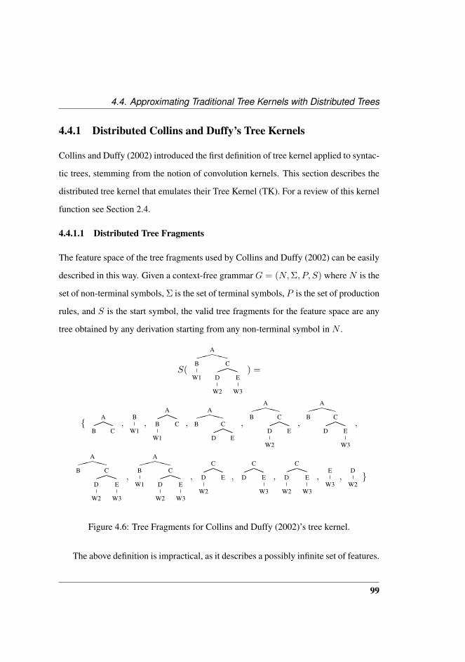
4.4. Approximating Traditional Tree Kernels with Distributed Trees

4.4.1 Distributed Collins and Duffy’s Tree Kernels

Collins and Duffy (2002) introduced the first definition of tree kernel applied to syntac-

tic trees, stemming from the notion of convolution kernels. This section describes the

distributed tree kernel that emulates their Tree Kernel (TK). For a review of this kernel

function see Section 2.4.

4.4.1.1 Distributed Tree Fragments

The feature space of the tree fragments used by Collins and Duffy (2002) can be easily

described in this way. Given a context-free grammar G = (N,Σ, P, S) where N is the

set of non-terminal symbols, Σ is the set of terminal symbols, P is the set of production

rules, and S is the start symbol, the valid tree fragments for the feature space are any

tree obtained by any derivation starting from any non-terminal symbol in N .

S(

AXX��

B

W1

CPP��

D

W2

E

W3

) =

{Aaa!!

B C,

B

W1,

Aaa!!

B

W1

C ,

AXX��

B Caa!!

D E

,

AXX��

B Caa!!

D

W2

E,

AXX��

B Caa!!

D E

W3

,

AXX��

B CPP��

D

W2

E

W3

,

AXX��

B

W1

CPP��

D

W2

E

W3

,

Caa!!

D

W2

E ,

Caa!!

D E

W3

,

CPP��

D

W2

E

W3

,E

W3,

D

W2}

Figure 4.6: Tree Fragments for Collins and Duffy (2002)’s tree kernel.

The above definition is impractical, as it describes a possibly infinite set of features.

99


Thus, a description of a function S(T ) that extracts the active subtrees from a given tree

T is generally preferred. Given a tree T , S(T ) contains any subtree of T which includes

more than one node, with the restriction that entire (not partial) rule productions must

be included. In other words, if node n in the original tree has children c1, . . . , cm, every

subtree containing n must include either the whole set of children c1, . . . , cm, or none

of them (i.e. having n as terminal node). Figure 4.6 gives an example.

For the formulation described in Section 2.4, the feature representing tree fragment

τ for a given tree T has weight:

ω =√λ|τ |−1

where |τ | is the number of non-terminal nodes of τ . In the original formulation (Collins

and Duffy, 2001), the contribution of tree fragment τ to the TK is λ|τ | giving a ω =√λ|τ | (see also Pighin and Moschitti (2010)). This difference is not relevant in the

overall theory of the distributed tree kernels.

The distributed tree fragments for the reduced version of this space are the depth-

first visits of the above subtrees. For example, given the tree fragments in Figure 4.6,

the corresponding distributed tree fragments for the first, the second, and the third tree

are: (;

A � (;

B �;

C)), (;

B �;

W1) and (;

A � ((;

B �;

W1) �;

C)).

4.4.1.2 Recursively Computing Distributed Trees

The structural recursive formulation for the computation of distributed trees;

T is the

following:;

T =∑

n∈N(T )

s(n) (4.6)

whereN(T ) is the node set of tree T and s(n) represents the sum of distributed vectors

for the subtrees of T rooted in node n. Function s(n) is recursively defined as follows:

100


• s(n) = ~0 if n is a terminal node.

• s(n) =;n � (

;c1 +

√λs(c1)) � . . . � (

;cm +

√λs(cm)) if n is a node with children

c1 . . . cm.

As in the TK, the decay factor λ decreases the weight of large tree fragments in the

final kernel value. With dynamic programming, the time complexity of this function is

linear O(|N(T )|) and the space complexity is d (where d is the size of the vectors in

Rd).

The overall theorem we need is the following.

Theorem 4.4.1. Given the ideal vector composition function �, the equivalence be-

tween Eq. 4.5 and Eq. 4.6 holds, i.e.:

;

T =∑

n∈N(T )

s(n) =∑

τi∈S(T )

ωif(τi)

We demonstrate Theorem 4.4.1 by showing that s(n) computes the weighted sum

of vectors for the subtrees rooted in n (see Theorem 4.4.2).

Definition 4.4.1. Let n be a node of tree T . We defineR(n) = {τ |τ is a subtree of T rooted in n}

We need to introduce a simple lemma, whose proof is trivial.

Lemma 4.4.1. Let τ be a tree with root node n. Let c1, . . . , cm be the children of n.

Then R(n) is the set of all trees τ ′ = (n, τ1, ..., τm) such that τi ∈ R(ci) ∪ {ci}.

Now we can show that function s(n) computes exactly the weighted sum of the

distributed tree fragments for all the subtrees rooted in n.

Theorem 4.4.2. Let n be a node of tree T . Then s(n) =∑

τ∈R(n)

√λ|τ |−1f(τ).

101


Proof. The theorem is proved by structural induction.

Basis. Let n be a terminal node. Then we have R (n) = ∅. Thus, by its definition,

s(n) = ~0 =∑

τ∈R(n)

√λ|τ |−1f(τ).

Step. Let n be a node with children c1, . . . , cm. The inductive hypothesis is then

s(ci) =∑

τ∈R(ci)

√λ|τ |−1f(τ). Applying the inductive hypothesis, the definition of

s(n) and the Property 4.3.2.3, we have

s(n) =;n �

(;c1 +

√λs(c1)

)� . . . �

(;cm +

√λs(cm)

)=

;n �

;c1 +

∑τ1∈R(c1)

√λ|τ1|f(τ1)

� . . . �;cm +

∑τm∈R(cm)

√λ|τm|f(τm)

=

;n �

∑τ1∈T1

√λ|τ1|f(τ1) � . . . �

∑τm∈Tm

√λ|τm|f(τm)

=∑

(n,τ1,...,τm)∈{n}×T1×...×Tm

√λ|τ1|+...+|τm|

;n � f(τ1) � . . . � f(τm)

where Ti is the setR(ci)∪{ci}. Thus, by means of Lemma 4.4.1 and the definition

of f , we can conclude that s(n) =∑

τ∈R(n)

√λ|τ |−1f(τ).

4.4.2 Distributed Subpath Tree Kernel

In this section, the Distributed Tree framework is applied to the Subpath Tree Kernel

(STK) for unordered trees. For a review of this kernel function see Section 2.4.1.2.

4.4.2.1 Distributed Tree Fragments for the Subpath Tree Kernel

A subpath of a tree is formally defined as a substring of a path from the root to one of

the leaves of the tree.

102


S(

AXX��

B

W1

CPP��

D

W2

E

W3

) = {A

B,

A

B

W1

,B

W1,

A

C

D

W2

,

C

D

W2

,

A

C

D

,A

C,

C

D,

D

W2,

A

C

E

W3

,

C

E

W3

,

A

C

E

,C

E,

E

W3, A,B,W1, C,D,E,W2,W3}

Figure 4.7: Tree Fragments for the subpath tree kernel.

Function S(T ) can be defined accordingly. Given a tree T , S(T ) contains any

sequence of symbols a0...an where ai is a direct descendant of ai−1 for any i > 0.

The distributed tree fragments are then:;a0 � (

;a1 � (...

;an)...)).

Figure 4.7 proposes an example of the above function. In Kimura et al. (2011), the

weight w for the subpath feature p for a given tree T is:

w = num(Tp)√λ|p|

where |p| is the length of subpath pi and num(Tp) is the number of times a subpath p

appears in tree T . The related distributed tree fragments can be easily derived.

4.4.2.2 Recursively Computing Distributed Trees for the Subpath Tree Kernel

As in the case of the TK, we can define a Distributed Tree representation;

T for tree

T such that the kernel function can be approximated by the explicit dot product, i.e.

STK(T1, T2) ≈;

T1 ·;

T2. In this case, each standard versor ~pi of the implicit feature

103


space Rm corresponds to a possible subpath pi. Thus, the Distributed Tree is:

;

T =∑

p∈P (T )

λ|p|;p (4.7)

where P (T ) is the set of subpaths of T and;p is the Distributed Tree Fragment vector

for subpath p. Subpaths can be seen as trees where each node has at most one child,

thus their DTF representation is the same.

Again, an explicit enumeration of the subpaths of a tree T is impractical, so an

efficient way to compute;

T is needed. The formulation in Eq. 4.6 is still valid, as long

as we define recursive function s(n) as follows:

s(n) =√λ

;n +

;n �

∑c∈C(n)

s(c)

(4.8)

where C(n) is the set of children of node n.

A theorem like Theorem 4.4.1 must be proved:

Theorem 4.4.3. Given the ideal vector composition function �, the following equiva-

lence holds:;

T =∑

n∈N(T )

s(n) =∑

p∈P (T )

√λ|p|

;p (4.9)

To prove Theorem 4.4.3, we introduce a definition and two simple lemmas, whose

proof is trivial. In the following, we will denote by (n|p) the concatenation of a node

n with a path p.

Definition 4.4.2. Let n be a node of a tree T . We define P (n) = {p|p is a subpath of

T starting with n}

Lemma 4.4.2. Let n be a tree node and C(n) the (possibly empty) set of its children.

Then P (n) = n ∪⋃

c∈C(n)

⋃p′∈P (c)

(n|p′).

104


Lemma 4.4.3. Let p = (n|p′) be the path given by the concatenation of node n and

path p′. Then;p =

;n �

;

p′.

Now we can show that function s(n) computes exactly the sum of the DTFs for all

the possible subpaths starting with n.


p∈P (n)

√λ|p|

;p .


Basis. Let n be a terminal node. Then we have P (n) = n. Thus, by its definition,

s(n) =√λ;n =

∑p∈P (n)

√λ|p|

;p .

Step. Let n be a node with children set C(n). The inductive hypothesis is then

∀c ∈ C(n).s(c) =∑

p∈P (c)

√λ|p|

;p . Applying the inductive hypothesis, the definition

of s(n) and Property 4.3.2.3, we have

s(n) =√λ

;n +

;n �

∑c∈C(n)

s(c)

=√λ

;n +

;n �

∑c∈C(n)

∑p∈P (c)

√λ|p|

;p

=√λ;n +

∑c∈C(n)

∑p∈P (c)

√λ|p|+1;n �;

p

Thus, by means of Lemmas 4.4.2 and 4.4.3, we can conclude that s(n) =∑

p∈P (n)

√λ|p|

;p .

105


Figure 4.8: Tree Fragments for the Route Tree Kernel.

4.4.3 Distributed Route Tree Kernel

The aim of this section is to introduce the distributed version of the Route Tree Kernel

(RTK) for positional trees. For a review of this kernel function see Section 2.4.1.2.

4.4.3.1 Distributed Tree Fragments for the Route Tree Kernel

The features considered by the RTK are the routes between a node ni and any of its

descendants nj , together with the label of node nj . An example is given in Figure 4.8,

that reports the tree we are using in this new form. The last node of the route has the

106


label whereas all the other nodes do not. The weight ω of route π(ni, nj) is:

ω =√λ|π(ni,nj)|

The transposition of these routes to distributed routes is straightforward. Indexes

Pn[e] are treated as new node labels. Thus, the distributed tree fragment associated

with the route π(n1, nk) ended by node nk is:

;πn1,nk = (

;

Pn1[(n1, n2)] � (

;

Pn2[(n2, n3)] � . . . �

;

Pnk−1[(nk−1, nk)])...) � ;

nk)

The Distributed Tree is then:

;

T =∑

π∈Π(T )

√λ|π|

;π (4.10)

where Π(T ) is the set of valid routes of T .

4.4.3.2 Recursively Computing Distributed Trees for the Route Tree Kernel

An efficient way to compute;

T is needed also in the case of the route features for a tree

T . The formulation in Eq. 4.6 is still valid, as long as we define recursive function s(n)

as follows:

s(n) =;n +√λ∑

c∈C(n)

;

Pn[(n, c)] � s(c) (4.11)

A theorem like Theorem 4.4.1 can be demonstrated to show that Eq. 4.6 with the

above definition of s(n) computes exactly the same as Eq. 4.5, where tree fragments

are the routes of the tree.

Theorem 4.4.5. Given the ideal vector composition function �, the following equiva-

lence holds:;

T =∑

n∈N(T )

s(n) =∑

π∈Π(T )

√λ|π|

;π (4.12)

107


To prove Theorem 4.4.5, we introduce a definition and a simple lemma, whose

proof is trivial.

Definition 4.4.3. Let n be a node of a tree T . We define Π(n) = {π(n,m)|m is a

descendant of n}.

Lemma 4.4.4. Let n be a tree node, m a child of n, and l a descendant of m. Then;πn,l =

;

Pn[(n,m)] � ;πm,l.

Now we can show that function s(n) computes exactly the sum of the DTFs for all

the possible routes starting in n.


π∈Π(n)

√λ|π|

;π .


Basis. Let n be a terminal node. Then we have Π(n) = πn,n. Thus, by its

definition, s(n) =;n =

;πn,n =

∑π∈Π(n)

√λ|π|

;π .

Step. Let n be a node with children set C(n). The inductive hypothesis is then

∀c ∈ C(n).s(c) =∑

π∈Π(c)

√λ|π|

;π . Applying the inductive hypothesis, the definition

of s(n) and Property 4.3.2.3, we have

s(n) =;n +√λ∑

c∈C(n)

;

Pn[(n, c)] � s(c)

=;πn,n +

√λ∑

c∈C(n)

;

Pn[(n, c)] �∑

π∈Π(c)

√λ|π|

;π

=;πn,n +

∑c∈C(n)

∑π∈Π(c)

√λ|π|+1

;

Pn[(n, c)] �;π

108

4.5. Evaluation and Experiments

Thus, by means of Lemma 4.4.4 and the definition of tree node descendants, we can

conclude that s(n) =∑

π∈Π(n)

√λ|π|

;π .

4.5 Evaluation and Experiments

Distributed tree kernels are an attractive counterpart to the traditional tree kernels, be-

ing linear and thus much faster to compute. But these kernels are an approximation

of the original ones. In the previous sections, we demonstrated that, given an ideal

vector composition function, the approximation is accurate. We have also shown that

approximations of the ideal vector composition functions exist. In this section, we

will investigate first how fast the distributed tree kernels are, and then how well they

approximate the original kernels.

The rest of the section is organized as follows. Section 4.5.2 analyzes the theoretical

and practical complexity of the distributed tree kernel, compared with the original tree

kernel (Collins and Duffy, 2002) and some of its improvements (Moschitti, 2006b;

Rieck et al., 2010; Pighin and Moschitti, 2010). Section 4.5.3 then proposes a direct

and task-based evaluation of how well DTKs approximate TKs.

4.5.1 Trees for the Experiments

The following experiments were performed using trees taken from actual linguistic

corpora and artificially generated. This section describes these two data classes.

4.5.1.1 Linguistic Parse Trees and Linguistic Tasks

For the task-based experiments, we used standard datasets for the two NLP tasks of

Question Classification (QC) and Recognizing Textual Entailment (RTE).

109


For QC, we used a standard training and test set3, where the test set are the 500

TREC 2001 test questions. To measure the task performance, we used a question

multi-classifier by combining n binary SVMs according to the ONE-vs-ALL scheme,

where the final output class is the one associated with the most probable prediction.

For RTE, we considered the corpora ranging from the first challenge to the fifth

(Dagan et al., 2006), except for the fourth, which has no training set. These sets are

referred to as RTE1-5. The dev/test distribution for RTE1-3, and RTE5 is respec-

tively 567/800, 800/800, 800/800, and 600/600 T-H pairs. We used these sets for the

traditional task of pair-based entailment recognition, where a pair of text-hypothesis

p = (t, h) is assigned a positive or negative entailment class.

As a final specification of the experimental setting, the Charniak’s parser (Charniak,

2000) was used to produce syntactic interpretations of sentences.

4.5.1.2 Artificial Trees

As in Rieck et al. (2010), many of the following experiments considered artificial trees

along with linguistic parse trees. The artificial trees are generated from a set of n node

labels, divided into terminal and non-terminal labels. A maximum out-degree d for

the tree nodes is chosen. The trees are generated recursively by building tree nodes

whose labels and numbers of children are picked at random, according to a uniform

distribution, until all tree branches end in a terminal node.

The Artificial Corpus of trees used in the following experiments is a set of 1000

trees generated randomly according to the described procedure. The label set contains

6 terminal and 6 non-terminal labels. The maximum out-degree is 3, and the trees are

composed of 30 nodes in average.

3The QC set is available at http://l2r.cs.uiuc.edu/˜cogcomp/Data/QA/QC/

110

http://l2r.cs.uiuc.edu/~cogcomp/Data/QA/QC/


Algorithm Tree preparation Learning ClassificationTime Space Time Space Time Space

TK - - O(n2) O(n2) O(n2) O(n2)FTK - - A(n) O(n2) A(n) O(n2)FTK-with-FS - - A(n) O(n2) k kATK - - O(n

2

qω) O(n2) O(n

2

qω) O(n2)

DTK O(n) d d d d d

Table 4.3: Computational time and space complexities for several tree kernel tech-niques: n is the tree dimension, qω is a speed-up factor, k is the size of the selectedfeature set, d is the dimension of space Rd, O(·) is the worst-case complexity, andA(·)is the average case complexity.

4.5.2 Complexity Comparison

In this section, we focus on how the distributed tree kernel affects the worst-case com-

plexity and the practical average computation time, when applied to the original tree

kernel (Collins and Duffy, 2002). For the other two kernels, we can draw similar con-

clusions as the ones we discuss here.

4.5.2.1 Analysis of the Worst-case Complexity

The initial formulation of the tree kernel by Collins and Duffy (2002) has a worst-

case complexity quadratic with respect to the number of nodes, both with respect to

time and space. Several studies have tried to propose methods for controlling the aver-

age execution time. Among them are the Fast Tree Kernels (FTK) by Moschitti (2006b)

and the Approximate Tree Kernels (ATK) by Rieck et al. (2010) (see Sec. 2.4.2).

With respect to these methods, Distributed Tree Kernels change the perspective,

since each kernel computation only consists in a vector dot product of constant com-

plexity, proportional to the dimension of the reduced space. The vector preparation still

111


has linear complexity with respect to the number of nodes, but this computation is only

performed once for each tree in the corpus. The differences of these approaches are

summarized in Table 4.3.

4.5.2.2 Average Computation Time

Since it is a relevant matter also for the Subpath Tree Kernel and the Route Tree Kernel,

and in order to have an idea of the practical application of the distributed tree kernels,

we measured the average computation time of FTK (Moschitti, 2006b) and DTK (with

vector size 8192) on a set of trees derived from the Question Classification corpus. As

these trees are parse trees, the FTK has an average linear complexity. The reported

results are then useful also to understand the behavior of the other two kernels. In fact,

the best implementations of the STK behave linearly with respect to the number of

nodes of the trees (Kimura and Kashima, 2012).

Figure 4.9 shows the relation between the computation time and the size of the

trees, computed as the total number of nodes in the two trees. As expected, DTK has

constant computation time, since it is independent of the size of the trees. On the

other hand, the computation time for FTK, while being lower for smaller trees, grows

very quickly with the tree size. The larger are the trees considered, the higher is the

computational advantage offered by using DTK instead of FTK.

4.5.3 Experimental Evaluation

In this section, we report on two experimental evaluations performed to estimate how

well the distributed tree kernels approximate the original tree kernels. The first set

of experiments is a direct evaluation: we compared the similarities computed by the

DTKs to those computed by the TKs. The second set of experiments is a task-based

112


0.001

0.01

0.1

1

10

0 40 80 120 160 200 240 280 320

Com

puta

tion

time

(ms)

Sum of nodes in the trees

FTKDTK

Figure 4.9: Computation time of FTK and DTK (with d = 8192) for tree pairs with anincreasing total number of nodes, on a 1.6 GHz CPU.

evaluation, where we investigated the behavior of the distributed tree kernels in two

NLP tasks.

4.5.3.1 Direct Comparison

These experiments test the ability of DTKs to emulate the corresponding TKs. We

compared the similarities derived by the traditional tree kernels with those derived

by the distributed versions of the kernels. For each set of trees (see Sec. 4.5.1), we

considered the Spearman’s correlation of DTK values with respect to TK values. Each

table reports the correlations for the three sets with different values of λ and with

113


Dim. 512 Dim. 1024 Dim. 2048 Dim. 4096 Dim. 8192Artificial λ=0.20 0.792 0.869 0.931 0.96 0.978Corpus λ=0.40 0.669 0.782 0.867 0.925 0.956

λ=0.60 0.34 0.454 0.59 0.701 0.812λ=0.80 0.06 0.058 0.075 0.141 0.306λ=1.00 0.018 0.017 -0.043 -0.019 0.112

QC λ=0.20 0.943 0.961 0.981 0.99 0.994Corpus λ=0.40 0.894 0.925 0.961 0.978 0.989

λ=0.60 0.571 0.621 0.73 0.804 0.88λ=0.80 0.165 0.148 0.246 0.299 0.377λ=1.00 0.037 0.014 0.06 0.108 0.107

RTE λ=0.20 0.969 0.983 0.991 0.996 0.998Corpus λ=0.40 0.849 0.888 0.919 0.943 0.961

λ=0.60 0.152 0.207 0.245 0.299 0.343λ=0.80 0.002 0.027 0.021 0.041 0.026λ=1.00 0.018 0.023 0.018 0.003 0

Table 4.4: Spearman’s correlation of DTK values with respect to TK values, on treestaken from the three data sets.

different vector space dimensions (d =1024, 2048, 4096, and 8192).

Distributed Tree Kernel The Spearman’s correlation results in Table 4.4 show that

DTK does not approximate adequately TK for λ = 1. Nonetheless, DTK’s perfor-

mances improve dramatically when parameter λ is reduced. The difference is mostly

notable on the linguistic corpora, thus highlighting once more DTK’s difficulty to cor-

rectly handle large trees. This is probably due to the influence of noise in the Dis-

tributed Tree representations.

Distributed Subpath Tree Kernel The Spearman’s correlation results for the Sub-

path Tree Kernel are reported in Table 4.5. In this case, the correlation is extremely

promising even for high values of λ. This is most likely because the feature space

114


Dim. 1024 Dim. 2048 Dim. 4096 Dim. 8192Artificial λ=0.20 0.958 0.979 0.992 0.995Corpus λ=0.40 0.945 0.968 0.988 0.993

λ=0.60 0.919 0.952 0.981 0.989λ=0.80 0.876 0.926 0.968 0.983λ=1.00 0.804 0.878 0.944 0.971

QC λ=0.20 0.994 0.997 0.999 0.999Corpus λ=0.40 0.991 0.997 0.998 0.999

λ=0.60 0.986 0.994 0.997 0.998λ=0.80 0.975 0.99 0.994 0.996λ=1.00 0.953 0.98 0.989 0.993

RTE λ=0.20 0.995 0.998 0.999 0.999Corpus λ=0.40 0.995 0.998 0.999 0.999

λ=0.60 0.994 0.998 0.999 0.999λ=0.80 0.992 0.996 0.998 0.998λ=1.00 0.986 0.993 0.996 0.997

Table 4.5: Spearman’s correlation of SDTK values with respect to STK values, takenon trees taken from the three data sets.

of STK is smaller than the one of TK, for trees of the same size. It should be noted

however that STK is commonly used over trees larger than the ones considered for this

experiment. Interestingly, though, the best performances are achieved on the linguistic

corpora, where DTK showed most limitations.

Distributed Route Tree Kernel The Spearman’s correlation results for the Route

Tree Kernel are reported in Table 4.6. The results are analogous to those obtained for

STK. This is not surprising, since their feature spaces are quite similar.

4.5.3.2 Task-based Experiments

In this section, we report on the experiments aimed at comparing the performance of

the distributed tree kernels with respect to the corresponding tree kernels on actual

115


Dim. 1024 Dim. 2048 Dim. 4096 Dim. 8192Artificial λ=0.20 0.962 0.982 0.994 0.995Corpus λ=0.40 0.953 0.974 0.991 0.992

λ=0.60 0.932 0.962 0.985 0.988λ=0.80 0.897 0.945 0.976 0.983λ=1.00 0.846 0.919 0.964 0.975

QC λ=0.20 0.992 0.998 0.999 1Corpus λ=0.40 0.99 0.997 0.999 0.999

λ=0.60 0.988 0.996 0.999 0.999λ=0.80 0.986 0.994 0.998 0.999λ=1.00 0.98 0.99 0.996 0.998

RTE λ=0.20 0.991 0.997 0.998 0.999Corpus λ=0.40 0.987 0.995 0.998 0.999

λ=0.60 0.981 0.991 0.996 0.998λ=0.80 0.97 0.984 0.992 0.996λ=1.00 0.948 0.968 0.985 0.992

Table 4.6: Spearman’s correlation of RDTK values with respect to RTK values, takenon trees taken from the three data sets.

linguistic tasks. The tasks considered are Question Classification (QC) and Recogniz-

ing Textual Entailment (RTE). For these experiments, we considered two versions of

the Distributed Tree Kernels, using two composition functions. We denote by DTK�

and DTK� the DTKs that use shuffled γ-product and shuffled circular convolution

respectively. An analogous notation is used for SDTK and RDTK. All Distributed Tree

Kernels rely on vectors of dimension 8192.

Performance on Question Classification task This experiment compared the per-

formances of DTKs with respect to TKs on the actual task of Question Classification.

The experimental setting is the one described in Section 4.5.1.1.

The results for the DTKs are shown in Figure 4.10. DTKs lead to worse perfor-

mances with respect to TK, but the gap is narrower for small values of λ ≤ 0.4.

116


60

65

70

75

80

85

90

0.2 0.4 0.6 0.8 1

Acc

urac

y

λ

TKDTK�DTK�

Figure 4.10: Performance on Question Classification task of TK, DTK� and DTK�

(d = 8192) for several values of λ.

These are the values usually adopted, since they produce better performances for the

task. Moreover, it can be noted that DTK� behaves better than DTK� for smaller

values of λ, while the opposite is true for larger values of λ. An explanation of this

phenomenon may be given in light of the results of the experiments in Section 4.3.4.3.

Since the norm of large vector compositions, using �, tends to drop greatly, their final

weight is smaller than expected. In other words, DTK� adds an implicit decay factor

to the explicit one. Thus, adopting larger values of λ affects DTK� less heavily than

it does for DTK� and TK itself.

117


83

83.5

84

84.5

85

85.5

86

86.5

87

0.2 0.4 0.6 0.8 1

Acc

urac

y

λ

STKSDTK�SDTK�

Figure 4.11: Performance on Question Classification task of STK, SDTK� andSDTK� (d = 8192) for several values of λ.

The results for the SDTKs and the RDTKs are shown in Figure 4.11 and Fig-

ure 4.12 respectively. SDTKs and RDTKs behave similarly to DTKs. Their perfor-

mances are very similar for small values of λ, while the gap increases for higher values

of λ. In these cases, STK and RTK seem to constantly gain accuracy when λ in-

creases. SDTK� and RDTK� achieve mostly stable performances, while SDTK�

and RDTK� show a performance decay for higher vales of λ. It should be noted,

though, that the range of accuracy obtained by Subpath and Route Tree Kernels is

much narrower than the one obtained by the Tree Kernel.

118


81

82

83

84

85

86

87

88

0.2 0.4 0.6 0.8 1

Acc

urac

y

λ

RTKRDTK�RDTK�

Figure 4.12: Performance on Question Classification task of RTK, RDTK� andRDTK� (d = 8192) for several values of λ.

Performance on Textual Entailment Recognition task For this experiment, the

setting is again the one described in Section 4.5.1.1. For our comparative analysis,

we used the syntax-based approach described in Moschitti and Zanzotto (2007) with

two kernel function schemes: (1) PKS(p1, p2) = KS(t1, t2) + KS(h1, h2); and, (2)

PKS+Lex(p1, p2) = Lex(t1, h1)Lex(t2, h2) + KS(t1, t2) + KS(h1, h2). Lex is the

lexical similarity between T andH , computed using WordNet-based metrics as in Cor-

ley and Mihalcea (2005). This feature is used in combination with the basic kernels and

it gives an important boost to their performances. KS is realized with TK, DTK�,

119


and DTK�. In the plots, the different PKS kernels are referred to as TK, DTK�,

and DTK� whereas the different PKS+Lex kernels are referred to as TK + Lex,

DTK� + Lex, and DTK� + Lex. Analogous notations are used for Subpath and

Route Tree Kernels. For the computation of the similarity feature Lex (Corley and

Mihalcea, 2005), we exploited the Jiang&Conrath distance (Jiang and Conrath, 1997)

computed using the wn::similarity package (Pedersen et al., 2004). As for the

case of the QC task, we considered several values of λ.

52

54

56

58

60

62

64

0.2 0.4 0.6 0.8 1

Acc

urac

y

λ

TK + Lex

DTK� + Lex

DTK� + Lex

TK

DTK�

DTK�

Figure 4.13: Performance on Recognizing Textual Entailment task of TK,DTK� andDTK� (d = 8192) for several values of λ. Each point is the average accuracy on the4 data sets.

Accuracy results for DTKs are reported in Figure 4.13. The results lead to con-

120


clusions similar to the ones drawn from the QC experiments. For λ ≤ 0.4, DTK�

and DTK� is similar to TK. Differences are not statistically significant except for

λ = 0.4, whereDTK� behaves better than TK (with p < 0.1). Statistical significance

is computed using the two-sample Student t-test. DTK� + Lex and DTK� + Lex

are statistically similar to TK + Lex for any value of λ.

55

56

57

58

59

60

61

62

63

0.2 0.4 0.6 0.8 1

Acc

urac

y

λ

STK + Lex

SDTK� + Lex

SDTK� + Lex

STK

SDTK�

SDTK�

Figure 4.14: Performance on Recognizing Textual Entailment task of STK, SDTK�

and SDTK� (d = 8192) for several values of λ. Each point is the average accuracyon the 4 data sets.

Accuracy results for SDTKs and RDTKs are reported in Figure 4.14 and Fig-

ure 4.15 respectively. The behavior is very similar to that of DTKs. In this case, the

performances are even slightly higher for the Distributed Kernels than for the original

121


55

56

57

58

59

60

61

62

63

0.2 0.4 0.6 0.8 1

Acc

urac

y

λ

RTK + Lex

RDTK� + Lex

RDTK� + Lex

RTK

RDTK�

RDTK�

Figure 4.15: Performance on Recognizing Textual Entailment task of RTK, RDTK�

and RDTK� (d = 8192) for several values of λ. Each point is the average accuracyon the 4 data sets.

Subpath and Route Kernels, and they seem to be less heavily affected by the values of

parameter λ.

122

5A Distributed Approach to a Symbolic

Task: Distributed Representation Parsing

Syntactic processing is widely considered an important activity in natural language

understanding (Chomsky, 1957). Research in natural language processing (NLP) pos-

itively exploits this hypothesis in models and systems. Syntactic features improve per-

formances in high level tasks such as question answering (Zhang and Lee, 2003), se-

mantic role labeling (Gildea and Jurafsky, 2002; Pradhan et al., 2005; Moschitti et al.,

2008; Collobert et al., 2011), paraphrase detection (Socher et al., 2011), and textual en-

tailment recognition (MacCartney et al., 2006; Wang and Neumann, 2007b; Zanzotto

et al., 2009).

Classification and learning algorithms are key components in the above models

and in current NLP systems. But these algorithms cannot directly use syntactic struc-

tures. The relevant parts of phrase structure trees or dependency graphs are explicitly

or implicitly stored in feature vectors, as explained in Chapter 4. Structural kernels al-

low to exploit high-dimensional spaces of syntactic tree fragments by concealing their

complexity. Then, even in kernel machines, symbolic syntactic structures act only as

proxies between the source sentences and the syntactic feature vectors. Syntactic struc-

tures are exploited to build or stand for these vectors, used by final algorithms when

learning and applying classifiers for high level tasks.

123

Chapter 5. A Distributed Approach to a Symbolic Task: DistributedRepresentation Parsing

In this chapter, we explore an alternative way to use syntax in feature spaces: the

Distributed Representation Parsers (DRP). The core of the idea is straightforward:

DRPs directly bridge the gap between sentences and syntactic feature spaces. DRPs

act as syntactic parsers and feature extractors at the same time. We leverage on the

distributed trees framework, introduced in Chapter 4, and on multiple linear regression

models, to learn linear DRPs from training data. DRPs are compared to the traditional

processing chain, i.e. a symbolic parser followed by the construction of distributed

trees, by performing experiments on the Penn Treebank data set (Marcus et al., 1993).

Results show that DRPs produce distributed trees significantly better than those ob-

tained by traditional methods, in the same non-lexicalized conditions, and competitive

with those obtained by traditional lexicalized methods. Moreover, it is shown that

DRPs are extremely faster than traditional methods.

The rest of the chapter is organized as follows. First, we introduce and describe the

DRP model, as a follow-up to the distributed trees framework (Section 5.1). Then, we

report on the experiments (Section 5.2).

5.1 Distributed Representation Parsers

In Chapter 4 we showed how the widespread use of tree kernels obfuscated the

fact that syntactic trees are ultimately used as vectors in learning algorithms. Stem-

ming from the research in Distributed Representations (Hinton et al., 1986; Bengio,

2009; Collobert et al., 2011; Socher et al., 2011), we proposed the distributed trees

(DT) framework as a solution to the problem of representing high-dimensional implicit

feature vectors through smaller but explicit vectors.

We showed through experimental results that distributed trees are good representa-

124

5.1. Distributed Representation Parsers

Figure 5.1: “Parsing” with distributed structures in perspective.

tions of syntactic trees, that we can use in the definition of distributed representation

parsers.

In the following, we sketch the idea of Distributed Representation “Parsers”. Then,

we describe how to build DRPs by combining a function that encodes sentences into

vectors and a linear regressor that can be induced from training data.

5.1.1 The Idea

The approach to using syntax in learning algorithms generally follows two steps: first,

parse sentences s with a symbolic parser (e.g. Collins (2003); Charniak (2000); Nivre

et al. (2007b)) and produce symbolic trees t; second, use tree kernels to exploit implicit

syntactic feature vectors, or use an encoder to build explicit ones. Figure 5.1 sketches

this idea, when the final vectors are the distributed trees;

t ∈ Rd introduced in Chap-

ter 4. The function used to build a distributed tree;

t from a tree t (see f(T ) in Eq. 4.3)

will be referred to as the Distributed Tree Encoder (DT).

125


Our proposal is to build a Distributed Representation “Parser” that directly maps

sentences s into the final vectors, i.e. the distributed trees. A DRP acts as follows (see

Fig. 5.1): first, a function D encodes sentence s into a distributed representation vector;s ∈ Rd; second, a function P transforms the input vector

;s into a distributed tree

;

t .

This second step is a vector to vector transformation and, in a wide sense, “parses” the

input sentence.

Given an input sentence s, a DRP is then a function defined as follows:

;

t = DRP (s) = P (D(s)) (5.1)

In this study, some functions D are designed and a linear function P is proposed,

designed to be a regressor that can be induced from training data. The used vector

space has d dimensions for both sentences;s and distributed trees

;

t ; but, in general,

the two spaces can be of different size.

The chosen distributed trees implementation is the one referring to the feature space

induced by the Collins and Duffy (2002) tree kernel, as described in Section 4.4.1.

The shuffled circular convolution is selected as the vector composition function �. We

experiment with two tree fragment sets: the non-lexicalized set Sno lex(t), where tree

fragments do not contain words, and the lexicalized set Slex(t), including all the tree

fragments. An example is given in Figure 5.2.

5.1.2 Building the Final Function

To build a DRP, the encoderD and the transformer P must be defined. In the following,

we present a non-lexicalized and a lexicalized model for the encoderD and we describe

how we can learn the transformer P by means of a linear regression model.

126


Sno lex(t) = {SPP��

NP VP,

VPPP��

V NP,

NP

PRP,

SPP��

NP

PRP

VP ,

SXX��

NP VPPP��

V NP

,

VPXX��

V NPaa!!

DT NN

, . . . }

Slex(t) = Sno lex(t) ∪ {

SPP��

NP

PRP

We

VP,

VP`` V

booked

NPaa!!

DT NN

,

VP`` V

booked

NPaa!!

DT

the

NN,

VP`` V

booked

NPPP��

DT NN

flight

, . . . }

Figure 5.2: Subtrees of the tree t in Fig. 5.1.

5.1.2.1 Sentence Encoders

Establishing good models to encode input sentences into vectors is the most difficult

challenge. These models should consider the kind of information that can lead to a

correct syntactic interpretation. Only in this way, the distributed representation parser

can act as a vector transformation module. Unlike in models such as Socher et al.

(2011), our encoder is required to represent the whole sentence as a fixed size vector.

In the following, a non-lexicalized model and a lexicalized model are proposed.

Non-lexicalized model The non-lexicalized model relies only on the pos-tags of the

sentences s: s = p1 . . . pn, where pi is the pos-tag associated with the i-th token of the

sentence. In the following we discuss how to encode this information in a Rd space.

The basic model D1(s) is the one that considers the bag-of-postags, that is:

D1(s) =∑i

;p i (5.2)

where;p i ∈ N is the vector for label pi, taken from the set of nearly orthonormal ran-

dom vectors N , as defined in Section 4.3.1. This is basically in line with the bag-of-

127


words model used in random indexing (Sahlgren, 2005). Due to the commutative prop-

erty of the sum and since vectors in N are nearly orthonormal: (1) two sentences with

the same set of pos-tags have the same vector; and, (2) the dot product between two

vectors, D1(s1) and D1(s2), representing sentences s1 and s2, approximately counts

how many pos-tags the two sentences have in common. The vector for the sentence in

Figure 5.1 is then:

D1(s) =;

PRP +;

V +;

DT +;

NN

The general non-lexicalized model that takes into account all n-grams of pos-tags,

up to length j, is then the following:

Dj(s) = Dj−1(s) +∑i

;p i � . . . �

;p i+j−1

where � is again the shuffled circular convolution. An n-gram pi . . . pi+j−1 of pos-tags

is represented as;p i � . . . �

;p i+j−1. Given the properties of the shuffled circular con-

volution, an n-gram of pos-tags is associated to a versor, as it composes j versors, and

two different n-grams have nearly orthogonal vectors. For example, vector D3(s) for

the sentence in Figure 5.1 is:

D3(s) =;

PRP +;

V +;

DT +;

NN +

;

PRP �;

V +;

V �;

DT +;

DT �;

NN +

;

PRP �;

V �;

DT +;

V �;

DT �;

NN

Lexicalized model Including lexical information is the hardest part of the overall

model, as it makes vectors denser in information. Here we propose an initial model

128


that is basically the same as the non-lexicalized model, but includes a vector represent-

ing the words in the unigrams. The equation representing sentences as unigrams is:

Dlex1 (s) =

∑i

;p i �

;wi

Vector;wi represents word wi and is taken from the set N of nearly orthonormal ran-

dom vectors. This guarantees that Dlex1 (s) is not lossy. Given a pair word-postag

(w, p), it is possible to know if the sentence contains this pair, as Dlex1 (s)×;

p �;w ≈ 1

if (w, p) is in sentence s and Dlex1 (s) × ;

p � ;w ≈ 0 otherwise. Other vectors for rep-

resenting words, e.g. distributional vectors or those obtained as look-up tables in deep

learning architectures (Collobert and Weston, 2008), do not guarantee this possibility.

The general equation for the lexicalized version of the sentence encoder follows:

Dlexj (s) = Dlex

j−1(s) +∑i

;p i � . . . �

;p i+j−1

This model is only an initial proposal in order to take into account lexical informa-

tion.

5.1.2.2 Learning Transformers with Linear Regression

The transformer P of the DRP (see Eq. 5.1) can be seen as a linear regressor:

;

t = D;s (5.3)

where D is a square matrix. This latter can be estimated having training sets (T,S) of

oracle vectors and sentence input vectors (;

t i,;s i) for sentences si. Oracle vectors are

the ones obtained by applying the Distributed Tree Encoder to the correct syntactic tree

129


for the sentence, provided by an oracle. Interpreting these sets as matrices, we need to

solve a linear system of equations, i.e.: T = DS.

An approximate solution can be computed using Principal Component Analysis

and Partial Least Square Regression1. This method relies on Moore-Penrose pseudo-

inversion (Penrose, 1955). Pseudo-inverse matrices S+ are obtained using singular

value decomposition (SVD). These matrices have the property SS+ = I. Using the

iterative method for computing SVD (Golub and Kahan, 1965), we can obtain different

approximations S+(k) of S+ considering k singular values. Final approximations of

DRP s are then: D(k) = TS+(k).

Matrices D are estimated by pseudo-inverting matrices representing input vectors

for sentences S. Given the different input representations for sentences, we can then

estimate different DRPs: DRP1 = TS+1 , DRP2 = TS+

2 , and so on. We need to

estimate the best value for k in a separate parameter estimation set.

5.2 Experiments

We evaluated three issues for assessing DRP models: first, the performance of DRPs

in reproducing oracle distributed trees (Section 5.2.2); second, the quality of the topol-

ogy of the vector spaces of distributed trees produced by DRPs (Section 5.2.3); and,

finally, the computation run time of DRPs (Section 5.2.4). Section 5.2.1 describes the

experimental set-up.

1An implementation of this method is available within the R statistical package (Mevik and Wehrens,2007).

130

5.2. Experiments

5.2.1 Experimental Set-up

Data The data sets were derived from the Wall Street Journal (WSJ) portion of the

English Penn Treebank data set (Marcus et al., 1993), using a standard data split for

training (sections 2-21PTtrain with 39,832 trees) and for testing (section 23PT23 with

2,416 trees). Section 24 PT24, with 1,346 trees, was used for parameter estimation.

We produced the final data sets of distributed trees with three different λ values:

λ=0, λ=0.2, and λ=0.4. For each λ, we have two versions of the data sets: a non-

lexicalized version (no lex), where syntactic trees are considered without words, and

a lexicalized version (lex), where words are considered. Oracle trees t are transformed

into oracle distributed trees;o using the Distributed Tree Encoder DT (see Fig. 5.1).

We experimented with two sizes of the distributed trees space Rd: 4096 and 8192.

We have designed the data sets to determine how DRPs behave with λ values rele-

vant for syntax-sensitive NLP tasks. Both tree kernels and distributed tree kernels have

the best performances in tasks such as question classification, semantic role labeling,

or textual entailment recognition with λ values in the range 0–0.4.

System Comparison We compared the DRPs against the original way of producing

distributed trees: distributed trees are obtained using the output of a symbolic parser

(SP) that is then transformed into a distributed tree using the DT with the appropriate

λ. We refer to this chain as the Distributed Symbolic Parser (DSP ). The DSP is then

the chain DSP (s) = Dtree(SP (s)). Figure 5.3 reports the definitions of the original

and the DRPs processing chain, along with the procedure leading to oracle trees.

As for the symbolic parser, we used Bikel’s version (Bikel, 2004) of Collins’ head-

driven statistical parser (Collins, 2003). For a correct comparison, we used the Bikel’s

131


Figure 5.3: Processing chains for the production of the distributed trees: translationof oracle trees, distributed trees with symbolic parsers, and distributed representationparsing.

parser with oracle part-of-speech tags. We experimented with two versions: (1) the

original lexicalized method DSPlex, i.e. the natural setting of the Collins/Bikel parser,

and (2) a fully non-lexicalized version DSPno lex that exploits only part-of-speech

tags. This latter version is obtained by removing words in input sentences and leaving

only part-of-speech tags. We trained these DSP s on PTtrain.

Parameter estimation DRPs have two basic parameters: (1) parameter k of the

pseudo-inverse, that is, the number of considered eigenvectors (see Sec. 5.1.2.2) and (2)

the maximum length j of the n-grams considered by the encoder Dj (see Sec. 5.1.2.1).

Parameter estimation was performed on the datasets derived from section PT24 by

maximizing a pseudo f-measure. Section 5.2.2 reports both the definition of the mea-

sure and the results of the parameter estimation.

132

5.2. Experiments

5.2.2 Parsing Performance

The first issue to explore is whether DRP s are actually good “distributed syntactic

parsers”. We compare DRP s against the distributed symbolic parsers by evaluating

how well these “distributed syntactic parsers” reproduce oracle distributed trees.

Method We define the pseudo f-measure, that is, a parsing performance measure

that aims to reproduce the traditional f-measure on the distributed trees. The pseudo

f-measure is defined as follows:

f(;

t ,;o ) =

2;

t ·;o

||;

t ||+ ||;o ||

where;

t is the system’s distributed tree and;o is the oracle distributed tree. This mea-

sure computes a score that is similar to traditional f-measure:;

t ·;o approximates true

positives, ||;

t || approximates the number of observations, and, finally, ||;o || approxi-

mates the number of expectations. We compute these two measures in a sentence-based

(i.e. vector-based) granularity. Results report average values.

Estimated parameters We estimated parameters k and j by training the different

DRP s on the PTtrain set and by maximizing the pseudo f-measure of the DRP s on

PT24. The best pair of parameters is j=3 and k=3000. For completeness, we report

also the best k values for the five different j we experimented with: k = 47 for j=1

(the number of linearly independent vectors representing pos-tags), k = 1300 for j=2,

k = 3000 for j=3, k = 4000 for j=4, and k = 4000 for j=5. For comparison, some

resulting tables report results for the different values of j.

133


dim Model λ = 0 λ = 0.2 λ = 0.4

4096

DRP1 0.6449 0.5697 0.4596DRP2 0.7843 0.7014 0.5766DRP3 0.8167 0.7335 0.6084DRP4 0.8039 0.7217 0.5966DRP5 0.7892 0.7069 0.5831DSPno lex 0.6504 0.5850 0.4806DSPlex 0.8129 0.7793 0.7099

8192DRP3 0.8228 0.7392 0.6139DSPno lex 0.6547 0.5891 0.4843DSPlex 0.8136 0.7795 0.7102

Table 5.1: Pseudo f-measure on PT23 of the DRP s (with different j) and the DSPon the non-lexicalized data sets with different λ values and with the two dimensions ofthe distributed tree space (4096 and 8192).

Model λ = 0 λ = 0.2 λ = 0.4

DRP3 0.6957 0.5997 0.0411DSPlex 0.9068 0.8558 0.6438

Table 5.2: Pseudo f-measure on PT23 of the DRP3 and the DSPlex on the lexicalizeddata sets with different λ values on the distributed tree space with 4096 dimensions.

134

5.2. Experiments

Results Table 5.1 reports the results of the first set of experiments on the non-lexicalized

data sets. The first block of rows (seven rows) reports the pseudo f-measure of the dif-

ferent methods on the distributed tree spaces with 4096 dimensions. The second block

(the last three rows) reports the performance on the space with 8192 dimensions. The

pseudo f-measure is computed on the PT23 set. Although we already selected j=3 as

the best parametrization (i.e. DRP3), the first five rows of the first block report the

results of the DRPs for five values of j. This gives an idea of how the different DRPs

behave. The last two rows of this block report the results of the two DSPs.

We can observe some important facts. First, DRP s exploiting 2-grams, 3-grams,

4-grams, and 5-grams of part-of-speech tags behave significantly better than the 1-

grams for all the values of λ. Distributed representation parsers need inputs that keep

trace of sequences of pos-tags of sentences. But these sequences tend to confuse the

model when too long. As expected, DRP3 behaves better than all the other DRPs.

Second, DRP3 behaves significantly better than the comparable original parsing chain

DSPno lex that uses only part-of-speech tags and no lexical information. This hap-

pens for all the values of λ. Third, DRP3 behaves similarly to DSPlex for λ=0. Both

parsers use oracle pos-tags to emit sentence interpretations but DSPlex also exploits

lexical information that DRP3 does not access. For λ=0.2 and λ=0.4, the more in-

formed DSPlex behaves significantly better than DRP3. But DRP3 still behaves sig-

nificantly better than the comparable DSPno lex. All these observations are valid also

for the results obtained for 8192 dimensions.

Table 5.2 reports the results of the second set of experiments on the lexicalized

data sets performed on a 4192-dimension space. The first row reports the pseudo f-

measure of DRP3 trained on the lexicalized model and the second row reports the

135


Output Model λ = 0 λ = 0.2 λ = 0.4

No lexDRP3 0.9490 0.9465 0.9408DSPno lex 0.9033 0.9001 0.8932DSPlex 0.9627 0.9610 0.9566

LexDRP3 0.9642 0.9599 0.0025DSPlex 0.9845 0.9817 0.9451

Table 5.3: Spearman’s Correlation between the oracle’s vector space and the systems’vector spaces, with dimension 4096. Average and standard deviation are on 100 trialson lists of 1000 sentence pairs.

results of DSPlex. In this case, DRP3 is not behaving well with respect to DSPlex.

The additional problem DRP3 has is that it has to reproduce input words in the output.

This greatly complicates the work of the distributed representation parser. But, as we

report in the next section, this preliminary result may be still satisfactory for λ=0 and

λ=0.2.

5.2.3 Kernel-based Performance

This experiment investigates howDRP s preserve the topology of the oracle vector

space. This correlation is an important quality factor of a distributed tree space. When

using distributed tree vectors in learning classifiers, whether;oi ·

;oj in the oracle’s vector

space is similar to;

ti ·;

tj in the DRP’s vector space is more important than whether;oi is similar to

;

ti (see Fig. 5.4). Sentences that are close using the oracle syntactic

interpretations should also be close using DRP vectors. The topology of the vector

space is more relevant than the actual quality of the vectors. The experiment on the

parsing quality in the previous section does not properly investigate this property, as

the performance of DRPs could be not sufficient to preserve distances among sentences.

136

5.2. Experiments

Figure 5.4: Topology of the resulting spaces derived with the three different methods:similarities between sentences.

Method We evaluate the coherence of the topology of two distributed tree spaces by

measuring the Spearman’s correlation between two lists of pairs of sentences (si, sj),

ranked according to the similarity between the two sentences. If the two lists of pairs

are highly correlated, the topology of the two spaces is similar. The different methods

and, thus, the different distributed tree spaces are compared against the oracle vector

space (see Fig. 5.4). Then, the first list always represents the oracle vector space and

ranks pairs (si, sj) according to;o i ·

;o j . The second list instead represents the space

obtained with a DSP or a DRP. Thus, it is respectively ranked with;

ti ·;

tj or;

ti ·;

tj . In

this way, we can comparatively evaluate the quality of the distributed tree vectors of

ourDRP s with respect to the other methods. We report average and standard deviation

of the Spearman’s correlation on 100 runs over lists of 1000 pairs. We used the testing

set PT23 for extracting vectors.

137


(a) Running time (b) Pseudo f-measure with λ=0.4

Figure 5.5: Performances with respect to the sentence length, with space dimension4092.

Results Table 5.3 reports results both on the non-lexicalized and on the lexicalized

data set. For the non-lexicalized data set we report three methods (DRP3, DSPno lex,

andDSPlex) and for the lexicalized dataset we report two methods (DRP3 andDSPlex).

Columns represent different values of λ. Experiments are carried out on the 4096-

dimension space. For the non-lexicalized data set, distributed representation parsers

behave significantly better than DSPno lex for all the values of λ. The upper-bound of

DSPlex is not so far. For the harder lexicalized data set, the difference between DRP3

and DSPlex is smaller than the one based on the parsing performance. Thus, we have

more evidence of the fact that we are in a good track. DRP s can substitute the DSP

in generating vector spaces of distributed trees that adequately approximate the space

defined by an oracle.

5.2.4 Running Time

138

5.2. Experiments

In this last experiment, we compared the running time of the DRP with respect to

the DSP . The analysis has been done on a dual-core processor and both systems are

implemented in the same programming language, i.e. Java. Figure 5.5a plots the run-

ning time of the DRP , the SP , and the full DSP = DT ◦ SP . The x-axis represents

the sentence length in words and the y-axis represents the running time in milliseconds.

The distance between SP and DSP shrinks as the plot is in a logarithmic scale. Fig-

ure 5.5b reports the pseudo f-measure of DRP , DSPlex, and DSPno lex, with respect

to the sentence length, on the non-lexicalized data set with λ=0.4.

We observe that DRP becomes extremely convenient for sentences larger than 10

words (see Fig. 5.5a) and the pseudo f-measure difference between the different meth-

ods is nearly constant for the different sentence lengths (see Fig. 5.5b). This test already

makes DRPs very appealing methods for real time applications. But, if we consider

that DRPs can run completely on Graphical Processing Units (GPUs), as dealing only

with matrix products, fast-Fourier transforms, and random generators, we can better

appreciate the potentials of the proposed methods.

139

6Conclusions and Future Work

Many fields of research require machine learning algorithms to work on structured

data. Thus, kernel methods such as the kernel machines are very useful, since they

allow for the definition of kernel functions. Kernel functions define an implicit feature

space, usually of very high dimensionality, and measure similarity as the dot product

of data instances mapped into the implicit feature space. One of the most frequently

recurring family of structure is the one of trees. The main interest of this thesis is

the use of syntactic trees in natural language processing tasks, but trees are used to

represent a wide variety of entities in several different fields, such as HTML documents

in computer security and proteins in biology.

Since their introduction, tree kernels have been very popular in the machine learn-

ing research community. Many different tree kernels have been proposed, defining new

feature spaces tailored to solve specific tasks and theoretic issues. At the same time,

new tree kernel algorithms have been proposed to tackle the high computation com-

plexity, which is quadratic in the size of the involved trees. After providing a brief

survey of kernels for structured data and, more specifically, of tree kernels, this thesis

proposed improvements on both of the mentioned research lines.

Firstly, we introduced a new kind of kernel, tailored to be applied in tasks where tree

pairs instead of single trees are considered, such as the textual entailment recognition

141

Chapter 6. Conclusions and Future Work

task of natural language processing. This kernel is built on top of the concept of tDAGs

(tripartite directed acyclic graphs), which are data structures used to represent a pair of

trees as a single graph, preserving information about correlated nodes. The modeled

feature space is the one of first order rules among trees. The proposed kernel on tDAGs

is, technically, a kernel on graphs. Complete kernels on generic graphs have been

proven to be NP-hard to compute. Nonetheless, we proposed an efficient algorithm

to compute the kernel, by exploiting the peculiar characteristics of tDAG structures.

We showed how the kernel on tDAGs is much more efficient than previously proposed

kernels for tree pairs. At the same time, this allows for a better use of the available

information, leading to higher performances on the textual entailment recognition task.

Second, we proposed the distributed tree kernels framework, as a means to strongly

reduce computational complexity of tree kernel functions. The idea for this framework

stems from the research field of distributed representations, concerning the representa-

tion of symbolic structures as distributed entities, i.e. points in vector spaces. Thus, the

main issue of the distributed tree kernels is the process of transforming trees into dis-

tributed trees, whereas the actual kernel computation consists in a simple dot product

between vectors of limited dimensionality. By introducing an ideal vector composition

function, satisfying some specific properties, we showed that the dot product between

two distributed trees computes an approximation of the corresponding tree kernel, as

long as the distributed trees are built in an appropriate manner. We showed that this ap-

proach can be applied to different kinds of tree kernel, defining different feature spaces,

and we introduced efficient algorithms to build distributed trees for the different ker-

nels. Then, we presented a broad empirical analysis concerning the ability of concrete

functions to approximate the ideal function properties and the degree of approxima-

142

tion of the resulting distributed tree kernels, with regard to the original ones. We can

observe that distributed tree kernels could allow on-line learning algorithms such as

those based on the perceptron (Rosenblatt, 1958) (e.g. the shifting perceptron model

(Cavallanti et al., 2007)) to use tree structures without any need to go for bounded

on-line learning models that select and discard vectors for memory constraint or time

complexity (Cavallanti et al., 2007; Dekel et al., 2005; Orabona et al., 2008).

Finally, we introduced a possible application of the distributed tree kernels frame-

work to the field of syntactic parsing algorithms. Syntactic parsing is a preliminary

step needed by every machine learning algorithm which makes use of syntactic trees.

Nonetheless, parsing is an expensive and not error free process. Since kernel methods

ultimately work on the implicit feature space representation of trees, we proposed a

way of directly obtaining the distributed representation of a syntactic tree, without go-

ing through the intermediate symbolic form. This process, named distributed represen-

tation parsing, requires sentences to be represented by a first, easy to obtain, distributed

representation. Then, an appropriately learned linear regressor is applied to produce the

final distributed tree representation. We presented an extensive analysis of the degree

of correlation of the syntactic tree space produced by the distributed representation

parser, with regard to the space produced by applying a traditional symbolic parser

and the original algorithm to build distributed trees. This novel path to use syntactic

structures in feature spaces opens interesting and unexplored possibilities. The tight

integration of parsing and feature vector generation lowers the computational cost of

producing distributed representations from trees, as circular convolution is not applied

on-line. Moreover, distributed representation parsers can contribute to treat syntax

in deep learning models in a uniform way. Deep learning models (Bengio, 2009) are

143


completely based on distributed representations. But, when applied to natural language

processing tasks (e.g. Collobert et al. (2011); Socher et al. (2011)), syntactic structures

are not represented in the neural networks in a distributed way. Syntactic information

is generally used by exploiting symbolic parse trees, and this information positively

impacts performances on final applications, e.g. in paraphrase detection (Socher et al.,

2011) and in semantic role labeling (Collobert et al., 2011).

6.1 Future Work

The themes introduced by this thesis lead to several open lines of research.

The algorithm introduced for the efficient computation of the kernel on tDAGs may

be adapted to work on more complex kinds of structures. Although the computation

of complete kernels on generic graphs is NP-hard, efficient algorithms might be found

allowing for the introduction of a kernel on generic directed acyclic graphs.

We have shown how the distributed tree kernels framework can be applied to re-

produce different tree kernels. Other than applying the framework to reproduce more

tree kernels, a further generalization can be explored, producing a distributed kernels

framework that can be applied to a wider range of structures, from strings to graphs.

Moreover, the representation of syntactic trees as distributed structures resembles

the distributional representation of the semantics of words. An integration of the two

approaches might lead to interesting advances in the popular research field of the com-

positional distributional semantics.

Distributed representation parsing could also benefit from the use of distributional

semantics information. In fact, our first approach does not adequately consider lexical

information, when building the initial distributed representation for a sentence. Using a

144

6.1. Future Work

more complex representation model, possibly including semantic information, can lead

to higher performances and may be better compared to traditional parsers. Finally the

integration of distributed representation parsers and deep learning models could result

in an interesting line of research.

145

Publications

Zanzotto, F. M. and Dell’Arciprete, L. (2009). Efficient kernels for sentence pair classi-

fication. In Conference on Empirical Methods on Natural Language Processing, pages

91–100

Zanzotto, F. M., Dell’arciprete, L., and Korkontzelos, Y. (2010). Rappresentazione dis-

tribuita e semantica distribuzionale dalla prospettiva dell’intelligenza artificiale. TEORIE

& MODELLI, XV II-III, 107–122

Zanzotto, F. M., Dell’Arciprete, L., and Moschitti, A. (2011). Efficient graph kernels

for textual entailment recognition. Fundamenta Informaticae, 107(2-3), 199 – 222

Zanzotto, F. M. and Dell’Arciprete, L. (2011a). Distributed structures and distributional

meaning. In Proceedings of the Workshop on Distributional Semantics and Composi-

tionality, pages 10–15, Portland, Oregon, USA. Association for Computational Lin-

guistics

Zanzotto, F. M. and Dell’Arciprete, L. (2011b). Distributed tree kernels rivaling tree

kernels in entailment recognition. In AI*IA Workshop on ”Learning by Reading in the

Real World”

DellArciprete, L., Murphy, B., and Zanzotto, F. (2012). Parallels between machine

and brain decoding. In F. Zanzotto, S. Tsumoto, N. Taatgen, and Y. Yao, editors,

Brain Informatics, volume 7670 of Lecture Notes in Computer Science, pages 162–

174. Springer Berlin Heidelberg

147


Zanzotto, F. M. and Dell’Arciprete, L. (2012). Distributed tree kernels. In Proceedings

of the 29th International Conference on Machine Learning (ICML-12), pages 193–200.

Omnipress

Zanzotto, F. M. and Dell’Arciprete, L. (2013). Transducing sentences to syntactic

feature vectors: an alternative way to ”parse”? In Proceedings of the Workshop on

Continuous Vector Space Models and their Compositionality, pages 40–49, Sofia, Bul-

garia. Association for Computational Linguistics

Dell’Arciprete, L. and Zanzotto, F. M. (2013). Distributed convolution kernels on

countable sets. Submitted to a journal

148

Bibliography

Aiolli, F., Da San Martino, G., and Sperduti, A. (2009). Route kernels for trees. In Pro-

ceedings of the 26th Annual International Conference on Machine Learning, ICML

’09, pages 17–24, New York, NY, USA. ACM.

Aleksander, I. and Morton, H. (1995). An introduction to neural computing. Interna-

tional Thomson Computer Press.

Bar-Haim, R., Dagan, I., Dolan, B., Ferro, L., Giampiccolo, D., and Magnini,

Bernardo Szpektor, I. (2006). The second PASCAL recognising textual entailment

challenge. In Proceedings of the Second PASCAL Challenges Workshop on Recog-

nising Textual Entailment, Venice, Italy.

Bengio, Y. (2009). Learning deep architectures for AI. Foundations and Trends in

Machine Learning, 2(1), 1–127.

Bikel, D. M. (2004). Intricacies of Collins’ parsing model. Comput. Linguist., 30,

479–511.

Bunescu, R. and Mooney, R. J. (2006). Subsequence kernels for re-

lation extraction. In Submitted to the Ninth Conference on Natural

Language Learning (CoNLL-2005), Ann Arbor, MI. Available at url-

http://www.cs.utexas.edu/users/ml/publication/ie.html.

Carpenter, B. (1992). The Logic of Typed Feature Structures. Cambridge University

Press, Cambridge, England.

Cavallanti, G., Cesa-Bianchi, N., and Gentile, C. (2007). Tracking the best hyperplane

with a simple budget perceptron. Machine Learning, 69(2-3), 143–167.

149

BIBLIOGRAPHY

Charniak, E. (2000). A maximum-entropy-inspired parser. In Proc. of the 1st NAACL,

pages 132–139, Seattle, Washington.

Chierchia, G. and McConnell-Ginet, S. (2001). Meaning and Grammar: An introduc-

tion to Semantics. MIT press, Cambridge, MA.

Chomsky, N. (1957). Aspect of Syntax Theory. MIT Press, Cambridge, Massachussetts.

Collins, M. (2003). Head-driven statistical models for natural language parsing. Com-

put. Linguist., 29(4), 589–637.

Collins, M. and Duffy, N. (2001). Convolution kernels for natural language. In NIPS,

pages 625–632.

Collins, M. and Duffy, N. (2002). New ranking algorithms for parsing and tagging:

Kernels over discrete structures, and the voted perceptron. In Proceedings of ACL02.

Collobert, R. and Weston, J. (2008). A unified architecture for natural language pro-

cessing: Deep neural networks with multitask learning. In International Conference

on Machine Learning, ICML.

Collobert, R., Weston, J., Bottou, L., Karlen, M., Kavukcuoglu, K., and Kuksa, P.

(2011). Natural language processing (almost) from scratch. J. Mach. Learn. Res.,

12, 2493–2537.

Corley, C. and Mihalcea, R. (2005). Measuring the semantic similarity of texts. In

Proc. of the ACL Workshop on Empirical Modeling of Semantic Equivalence and

Entailment, pages 13–18. Association for Computational Linguistics, Ann Arbor,

Michigan.

150

BIBLIOGRAPHY

Cortes, C. and Vapnik, V. (1995). Support vector networks. Machine Learning, 20,

1–25.

Cristianini, N. and Shawe-Taylor, J. (2000). An Introduction to Support Vector Ma-

chines and Other Kernel-based Learning Methods. Cambridge University Press.

Cristianini, N., Shawe-Taylor, J., and Lodhi, H. (2002). Latent semantic kernels. J.

Intell. Inf. Syst., 18(2-3), 127–152.

Cumby, C. and Roth, D. (2002). Learning with feature description logics. In ILP, pages

32–47.

Cumby, C. and Roth, D. (2003). On kernel methods for relational learning. In ICML,

pages 107–114.

Dagan, I. and Glickman, O. (2004). Probabilistic textual entailment: Generic applied

modeling of language variability. In Proceedings of the Workshop on Learning Meth-

ods for Text Understanding and Mining, Grenoble, France.

Dagan, I., Glickman, O., and Magnini, B. (2006). The PASCAL recognising textual

entailment challenge. In Q.-C. et al., editor, LNAI 3944: MLCW 2005, pages 177–

190, Milan, Italy. Springer-Verlag.

Dang, H. T. (2005). Overview of DUC 2005. In Proceedings of the 2005 Document

Understanding Workshop.

Dasgupta, S. and Gupta, A. (1999). An elementary proof of the Johnson-Lindenstrauss

lemma. Technical Report TR-99-006, ICSI, Berkeley, California.

151

BIBLIOGRAPHY

de Marneffe, M.-C., MacCartney, B., Grenager, T., Cer, D., Rafferty, A., and D. Man-

ning, C. (2006). Learning to distinguish valid textual entailments. In Proceedings

of the Second PASCAL Challenges Workshop on Recognising Textual Entailment,

Venice, Italy.

Deerwester, S., Dumais, S. T., Furnas, G. W., L, T. K., and Harshman, R. (1990). In-

dexing by latent semantic analysis. Journal of the American Society for Information

Science, 41, 391–407.

Dekel, O., Shalev-Shwartz, S., and Singer, Y. (2005). The forgetron: A kernel-based

perceptron on a fixed budget. In In Advances in Neural Information Processing

Systems 18, pages 259–266. MIT Press.

Dell’Arciprete, L. and Zanzotto, F. M. (2013). Distributed convolution kernels on

countable sets. Submitted to a journal.

DellArciprete, L., Murphy, B., and Zanzotto, F. (2012). Parallels between machine and

brain decoding. In F. Zanzotto, S. Tsumoto, N. Taatgen, and Y. Yao, editors, Brain

Informatics, volume 7670 of Lecture Notes in Computer Science, pages 162–174.

Springer Berlin Heidelberg.

Dussel, P., Gehl, C., Laskov, P., and Rieck, K. (2008). Incorporation of application

layer protocol syntax into anomaly detection. In Proceedings of the 4th International

Conference on Information Systems Security, ICISS ’08, pages 188–202, Berlin,

Heidelberg. Springer-Verlag.

152

BIBLIOGRAPHY

Eisner, J. (2003). Learning non-isomorphic tree mappings for machine translation.

In Proceedings of the 41st Annual Meeting of the Association for Computational

Linguistics (ACL), Companion Volume, pages 205–208, Sapporo.

Gartner, T. (2002). Exponential and geometric kernels for graphs. In NIPS Workshop

on Unreal Data: Principles of Modeling Nonvectorial Data.

Gartner, T. (2003). A survey of kernels for structured data. SIGKDD Explorations.

Gartner, T., Flach, P., and Wrobel, S. (2003). On graph kernels: Hardness results and

efficient alternatives. Lecture notes in computer science, pages 129–143.

Gildea, D. and Jurafsky, D. (2002). Automatic Labeling of Semantic Roles. Computa-

tional Linguistics, 28(3), 245–288.

Golub, G. and Kahan, W. (1965). Calculating the singular values and pseudo-inverse

of a matrix. Journal of the Society for Industrial and Applied Mathematics, Series

B: Numerical Analysis, 2(2), 205–224.

Grinberg, D., Lafferty, J., and Sleator, D. (1996). A robust parsing algorithm for link

grammar. In 4th International workshop on parsing tecnologies, Prague.

Haghighi, A. D., Ng, A. Y., and Manning, C. D. (2005). Robust textual inference via

graph matching. In Proceedings of the conference on Human Language Technology

and Empirical Methods in Natural Language Processing, HLT ’05, pages 387–394,

Stroudsburg, PA, USA. Association for Computational Linguistics.

Harabagiu, S. and Hickl, A. (2006). Methods for using textual entailment in open-

domain question answering. In Proceedings of the 21st International Conference on

153

BIBLIOGRAPHY

Computational Linguistics and 44th Annual Meeting of the Association for Compu-

tational Linguistics, pages 905–912, Sydney, Australia. Association for Computa-

tional Linguistics.

Harabagiu, S., Hickl, A., and Lacatusu, F. (2007). Satisfying information needs with

multi-document summaries. Information Processing & Management, 43(6), 1619 –

1642. Text Summarization.

Hashimoto, K., Takigawa, I., Shiga, M., Kanehisa, M., and Mamitsuka, H. (2008).

Mining significant tree patterns in carbohydrate sugar chains. Bioinformatics, 24,

i167–i173.

Haussler, D. (1999). Convolution kernels on discrete structures. Technical report,

University of California at Santa Cruz.

Hecht-Nielsen, R. (1994). Context vectors: general purpose approximate meaning

representations self-organized from raw data. Computational Intelligence: Imitating

Life, IEEE Press, pages 43–56.

Hickl, A., Williams, J., Bensley, J., Roberts, K., Rink, B., and Shi, Y. (2006). Rec-

ognizing textual entailment with LCCs GROUNDHOG system. In B. Magnini and

I. Dagan, editors, Proceedings of the Second PASCAL Recognizing Textual Entail-

ment Challenge, Venice, Italy. Springer-Verlag.

Hinton, G. E., McClelland, J. L., and Rumelhart, D. E. (1986). Distributed represen-

tations. In D. E. Rumelhart and J. L. McClelland, editors, Parallel Distributed Pro-

cessing: Explorations in the Microstructure of Cognition. Volume 1: Foundations.

MIT Press, Cambridge, MA.

154

BIBLIOGRAPHY

Jiang, J. J. and Conrath, D. W. (1997). Semantic similarity based on corpus statistics

and lexical taxonomy. In Proc. of the 10th ROCLING, pages 132–139. Tapei, Taiwan.

John, G. H. and Langley, P. (1995). Estimating continuous distributions in bayesian

classifiers. In Proceedings of the Eleventh conference on Uncertainty in artificial

intelligence, UAI’95, pages 338–345, San Francisco, CA, USA. Morgan Kaufmann

Publishers Inc.

Johnson, W. and Lindenstrauss, J. (1984). Extensions of Lipschitz mappings into a

Hilbert space. Contemp. Math., 26, 189–206.

Kainen, P. C. and Kurkova, V. (1993). Quasiorthogonal dimension of euclidean spaces.

Applied Mathematics Letters, 6(3), 7 – 10.

Kashima, H. and Koyanagi, T. (2002). Kernels for semi-structured data. In Proceedings

of the Nineteenth International Conference on Machine Learning, ICML ’02, pages

291–298, San Francisco, CA, USA. Morgan Kaufmann Publishers Inc.

Kashima, H., Tsuda, K., and Inokuchi, A. (2003). Marginalized kernels between la-

beled graphs. In Proceedings of the Twentieth International Conference on Machine

Learning, pages 321–328. AAAI Press.

Kimura, D. and Kashima, H. (2012). Fast computation of subpath kernel for trees.

CoRR, abs/1206.4642.

Kimura, D., Kuboyama, T., Shibuya, T., and Kashima, H. (2011). A subpath kernel for

rooted unordered trees. In J. Huang, L. Cao, and J. Srivastava, editors, Advances in

Knowledge Discovery and Data Mining, volume 6634 of Lecture Notes in Computer

Science, pages 62–74. Springer Berlin / Heidelberg.

155

BIBLIOGRAPHY

Kobler, J., Schoning, U., and Toran, J. (1993). The graph isomorphism problem: its

structural complexity. Birkhauser Verlag, Basel, Switzerland, Switzerland.

Kondor, R. I. and Lafferty, J. (2002). Diffusion kernels on graphs and other discrete

structures. In In Proceedings of the ICML, pages 315–322.

Leslie, C., Eskin, E., and Noble, W. S. (2002). The spectrum kernel: a string kernel

for SVM protein classification. Pacific Symposium On Biocomputing, 575(50), 564–

575.

Li, W., Ong, K.-L., Ng, W.-K., and Sun, A. (2005). Spectral kernels for classification.

In Proceedings of the 7th international conference on Data Warehousing and Knowl-

edge Discovery, DaWaK’05, pages 520–529, Berlin, Heidelberg. Springer-Verlag.

Lin, D. and Pantel, P. (2001). DIRT-discovery of inference rules from text. In Proceed-

ings of the ACM Conference on Knowledge Discovery and Data Mining (KDD-01),

San Francisco, CA.

Lodhi, H., Saunders, C., Shawe-Taylor, J., Cristianini, N., and Watkins, C. (2002). Text

classification using string kernels. J. Mach. Learn. Res., 2, 419–444.

MacCartney, B., Grenager, T., de Marneffe, M.-C., Cer, D., and Manning, C. D. (2006).

Learning to recognize features of valid textual entailments. In Proceedings of the

Human Language Technology Conference of the NAACL, Main Conference, pages

41–48, New York City, USA. Association for Computational Linguistics.

Marcus, M. P., Santorini, B., and Marcinkiewicz, M. A. (1993). Building a large an-

notated corpus of English: The Penn Treebank. Computational Linguistics, 19,

313–330.

156

BIBLIOGRAPHY

Mercer, J. (1909). Functions of positive and negative type, and their connection with

the theory of integral equations. Philosophical Transactions of the Royal Society

of London. Series A, Containing Papers of a Mathematical or Physical Character,

209(441-458), 415–446.

Mevik, B.-H. and Wehrens, R. (2007). The pls package: Principal component and

partial least squares regression in R. Journal of Statistical Software, 18(2), 1–24.

Minnen, G., Carroll, J., and Pearce, D. (2001). Applied morphological processing of

English. Natural Language Engineering, 7(3), 207–223.

Mitchell, T. M. (1997). Machine Learning. McGraw-Hill, Inc., New York, NY, USA,

1 edition.

Moschitti, A. (2004). A study on convolution kernels for shallow semantic parsing. In

proceedings of the ACL, Barcelona, Spain.

Moschitti, A. (2006a). Efficient Convolution Kernels for Dependency and Constituent

Syntactic Trees. In Proceedings of The 17th European Conference on Machine

Learning, Berlin, Germany.

Moschitti, A. (2006b). Making tree kernels practical for natural language learning. In

Proceedings of EACL’06, Trento, Italy.

Moschitti, A. and Zanzotto, F. M. (2007). Fast and effective kernels for relational

learning from texts. In Proceedings of the International Conference of Machine

Learning (ICML), Corvallis, Oregon.

Moschitti, A., Pighin, D., and Basili, R. (2008). Tree kernels for semantic role labeling.

Computational Linguistics, 34(2), 193–224.

157

BIBLIOGRAPHY

MUC-7 (1997). Proceedings of the seventh message understanding conference (MUC-

7). In Columbia, MD. Morgan Kaufmann.

Muller, K.-R., Mika, S., Ratsch, G., Tsuda, K., and Scholkopf, B. (2001). An intro-

duction to kernel-based learning algorithms. IEEE TRANSACTIONS ON NEURAL

NETWORKS, 12(2), 181–201.

Nivre, J., Hall, J., Kubler, S., McDonald, R., Nilsson, J., Riedel, S., and Yuret, D.

(2007a). The CoNLL 2007 shared task on dependency parsing. In Proceedings of the

CoNLL Shared Task Session of EMNLP-CoNLL 2007, pages 915–932. Association

for Computational Linguistics, Prague, Czech Republic.

Nivre, J., Hall, J., Nilsson, J., Chanev, A., Eryigit, G., Kubler, S., Marinov, S., and

Marsi, E. (2007b). Maltparser: A language-independent system for data-driven de-

pendency parsing. Natural Language Engineering, 13(2), 95–135.

Orabona, F., Keshet, J., and Caputo, B. (2008). The projectron: a bounded kernel-based

perceptron. In W. W. Cohen, A. McCallum, and S. T. Roweis, editors, Machine

Learning, Proceedings of the Twenty-Fifth International Conference (ICML 2008),

Helsinki, Finland, June 5-9, 2008, volume 307 of ACM International Conference

Proceeding Series, pages 720–727. ACM.

Paass, G., Leopold, E., Larson, M., Kindermann, J., and Eickeler, S. (2002). SVM

classification using sequences of phonemes and syllables. In Proceedings of the

6th European Conference on Principles of Data Mining and Knowledge Discovery,

PKDD ’02, pages 373–384, London, UK, UK. Springer-Verlag.

158

BIBLIOGRAPHY

Pantel, p. and Pennacchiotti, M. (2006). Espresso: A bootstrapping algorithm for

automatically harvesting semantic relations. In Proceedings of the 21st Coling and

44th ACL, Sydney, Australia.

Pedersen, T., Patwardhan, S., and Michelizzi, J. (2004). WordNet::Similarity - measur-

ing the relatedness of concepts. In Proc. of 5th NAACL. Boston, MA.

Penrose, R. (1955). A generalized inverse for matrices. In Proc. Cambridge Philo-

sophical Society.

Peas, A., lvaro Rodrigo, and Verdejo, F. (2007). Overview of the answer validation

exercise 2007. In C. Peters, V. Jijkoun, T. Mandl, H. Mller, D. W. Oard, A. Peas,

V. Petras, and D. Santos, editors, CLEF, volume 5152 of Lecture Notes in Computer

Science, pages 237–248. Springer.

Pighin, D. and Moschitti, A. (2010). On reverse feature engineering of syntactic tree

kernels. In Conference on Natural Language Learning (CoNLL-2010), Uppsala,

Sweden.

Plate, T. A. (1994). Distributed Representations and Nested Compositional Structure.

Ph.D. thesis.

Pollard, C. and Sag, I. (1994). Head-driven Phrase Structured Grammar. Chicago

CSLI, Stanford.

Pradhan, S., Ward, W., Hacioglu, K., Martin, J. H., and Jurafsky, D. (2005). Semantic

role labeling using different syntactic views. In ACL ’05: Proceedings of the 43rd

Annual Meeting on Association for Computational Linguistics, pages 581–588. As-

sociation for Computational Linguistics, Morristown, NJ, USA.

159

BIBLIOGRAPHY

Quinlan, R. J. (1993). C4.5: Programs for Machine Learning (Morgan Kaufmann

Series in Machine Learning). Morgan Kaufmann.

Raina, R., Haghighi, A., Cox, C., Finkel, J., Michels, J., Toutanova, K., MacCartney,

B., de Marneffe, M.-C., Christopher, M., and Ng, A. Y. (2005). Robust textual infer-

ence using diverse knowledge sources. In Proceedings of the 1st Pascal Challenge

Workshop, Southampton, UK.

Rieck, K., Krueger, T., Brefeld, U., and Muller, K.-R. (2010). Approximate tree ker-

nels. J. Mach. Learn. Res., 11, 555–580.

Rosenblatt, F. (1958). The perceptron: a probabilistic model for information storage

and organization in the brain. Psychological Reviews, 65(6), 386–408.

Rousu, J. and Shawe-Taylor, J. (2005). Efficient computation of gapped substring

kernels on large alphabets. J. Mach. Learn. Res., 6, 1323–1344.

Rumelhart, D. E. and McClelland, J. L. (1986). Parallel Distributed Processing: Ex-

plorations in the Microstructure of Cognition : Foundations (Parallel Distributed

Processing). MIT Press.

Sahlgren, M. (2005). An introduction to random indexing. In Proceedings of the

Methods and Applications of Semantic Indexing Workshop at the 7th International

Conference on Terminology and Knowledge Engineering (TKE), Copenhagen, Den-

mark.

Sahlgren, M., Holst, A., and Kanerva, P. (2008). Permutations as a means to encode

order in word space. In V. Sloutsky, B. Love, and K. Mcrae, editors, Proceedings

160

BIBLIOGRAPHY

of the 30th Annual Conference of the Cognitive Science Society, pages 1300–1305.

Cognitive Science Society, Austin, TX.

Scholkopf, B. (1997). Support Vector Learning.

Shin, K. and Kuboyama, T. (2010). A generalization of Haussler’s convolution kernel:

mapping kernel and its application to tree kernels. J. Comput. Sci. Technol., 25(5),

1040–1054.

Shin, K., Cuturi, M., and Kuboyama, T. (2011). Mapping kernels for trees. In L. Getoor

and T. Scheffer, editors, Proceedings of the 28th International Conference on Ma-

chine Learning (ICML-11), ICML ’11, pages 961–968, New York, NY, USA. ACM.

Socher, R., Huang, E. H., Pennington, J., Ng, A. Y., and Manning, C. D. (2011). Dy-

namic pooling and unfolding recursive autoencoders for paraphrase detection. In

Advances in Neural Information Processing Systems 24.

Sun, J., Zhang, M., and Tan, C. L. (2011). Tree sequence kernel for natural language.

Suzuki, J. and Isozaki, H. (2006). Sequence and tree kernels with statistical feature

mining. In Advances in Neural Information Processing Systems 18, pages 1321–

1328. MIT Press.

Suzuki, J., Hirao, T., Sasaki, Y., and Maeda, E. (2003). Hierarchical directed acyclic

graph kernel: Methods for structured natural language data. In In Proceedings of the

41st Annual Meeting of the Association for Computational Linguistics, pages 32–39.

Tesniere, L. (1959). Elements de syntaxe structurale. Klincksiek, Paris, France.

Vapnik, V. (1995). The Nature of Statistical Learning Theory. Springer.

161

BIBLIOGRAPHY

Vert, J.-P. (2002). A tree kernel to analyse phylogenetic profiles. Bioinformatics,

18(suppl 1), S276–S284.

Voorhees, E. M. (2001). The TREC question answering track. Nat. Lang. Eng., 7(4),

361–378.

Wang, J. (1997). Average-case computational complexity theory. pages 295–328.

Wang, R. and Neumann, G. (2007a). Recognizing textual entailment using a subse-

quence kernel method. In Proceedings of the Twenty-Second AAAI Conference on

Artificial Intelligence (AAAI-07), July 22-26, Vancouver, Canada.

Wang, R. and Neumann, G. (2007b). Recognizing textual entailment using sentence

similarity based on dependency tree skeletons. In Proceedings of the ACL-PASCAL

Workshop on Textual Entailment and Paraphrasing, pages 36–41, Prague. Associa-

tion for Computational Linguistics.

Zanzotto, F. M. and Dell’Arciprete, L. (2009). Efficient kernels for sentence pair clas-

sification. In Conference on Empirical Methods on Natural Language Processing,

pages 91–100.

Zanzotto, F. M. and Dell’Arciprete, L. (2011a). Distributed structures and distribu-

tional meaning. In Proceedings of the Workshop on Distributional Semantics and

Compositionality, pages 10–15, Portland, Oregon, USA. Association for Computa-

tional Linguistics.

Zanzotto, F. M. and Dell’Arciprete, L. (2011b). Distributed tree kernels rivaling tree

kernels in entailment recognition. In AI*IA Workshop on ”Learning by Reading in

the Real World”.

162

BIBLIOGRAPHY

Zanzotto, F. M. and Dell’Arciprete, L. (2012). Distributed tree kernels. In Proceedings

of the 29th International Conference on Machine Learning (ICML-12), pages 193–

200. Omnipress.

Zanzotto, F. M. and Dell’Arciprete, L. (2013). Transducing sentences to syntactic

feature vectors: an alternative way to ”parse”? In Proceedings of the Workshop on

Continuous Vector Space Models and their Compositionality, pages 40–49, Sofia,

Bulgaria. Association for Computational Linguistics.

Zanzotto, F. M. and Moschitti, A. (2006). Automatic learning of textual entailments

with cross-pair similarities. In Proceedings of the 21st Coling and 44th ACL, pages

401–408. Sydney, Australia.

Zanzotto, F. M. and Moschitti, A. (2007). Experimenting a ”General Purpose” Textual

Entailment Learner in AVE, volume 4730, pages 510–517. Springer, DEU.

Zanzotto, F. M., Pennacchiotti, M., and Pazienza, M. T. (2006). Discovering asymmet-

ric entailment relations between verbs using selectional preferences. In Proceedings

of the 21st Coling and 44th ACL, Sydney, Australia.

Zanzotto, F. M., Pennacchiotti, M., and Moschitti, A. (2009). A machine learning ap-

proach to textual entailment recognition. NATURAL LANGUAGE ENGINEERING,

15-04, 551–582.

Zanzotto, F. M., Dell’arciprete, L., and Korkontzelos, Y. (2010). Rappresentazione

distribuita e semantica distribuzionale dalla prospettiva dell’intelligenza artificiale.

TEORIE & MODELLI, XV II-III, 107–122.

163

BIBLIOGRAPHY

Zanzotto, F. M., Dell’Arciprete, L., and Moschitti, A. (2011). Efficient graph kernels

for textual entailment recognition. Fundamenta Informaticae, 107(2-3), 199 – 222.

Zhang, D. and Lee, W. S. (2003). Question classification using support vector ma-

chines. In Proceedings of the 26th annual international ACM SIGIR conference on

Research and development in information retrieval, SIGIR ’03, pages 26–32, New

York, NY, USA. ACM.

164

EXPLOITING STRUCTURED DATA FOR MACHINE LEARNING ... · 3.1 Machine Learning for Textual Entailment...

Documents

Transcript of EXPLOITING STRUCTURED DATA FOR MACHINE LEARNING ... · 3.1 Machine Learning for Textual Entailment...